Firm Size and Complementarity betweenGeography and Products

Yoko Shibuya∗

Stanford University

December 5, 2021Preliminary

Abstract

I develop a model of heterogeneous multi-product firms operatingin multiple markets that comprise consumers with heterogeneous tastes.In the model, firms choose two extensive margins: product scope (howmany products to sell) and geographic scope (how many markets tosell products to). Their decisions on product and geographic scopesinteract in two ways: (1) the more products firms sell and the largerprofit they expect, the more likely they are to enter a market, and (2)the more markets they enter, the greater variety of products they sellto cater to heterogeneous local tastes. I estimate the model to matchmoments in the Japanese barcode-level transaction data using the sim-ulated method of moments. I run counterfactual exercises and find thateliminating either product or geographic scope underestimates firm sizevariations by 86% to 94% due to the interaction between the two mar-gins. Furthermore, I analyze how missing one of the margins affects thewelfare implication of size-dependent policies, taking an actual SMEsubsidy in Japan as an example. The results indicate that omitting theproduct scope margin underestimates the welfare costs of the subsidyby more than half.

∗I am deeply indebted to Pete Klenow, Kyle Bagwell, Matthew Grant, and Takeo Hoshi fortheir invaluable guidance and support. I am grateful to Adrien Auclert, Chad Jones, MartinSchneider, Monika Piazzesi, Andres Rodrıguez-Clare, Christopher Tonetti, and participantsin IO, international trade, and macro seminars at Stanford University for their helpful dis-cussions. I am grateful to Freeman Spogli Institute for International Studies and SIEPR atStanford University for financial support for this project.

2 YOKO SHIBUYA

1. Introduction

In many countries, markets consist of a few large firms and many small

firms. The same is true for the Japanese manufacturing industry, where

small and medium enterprises (SMEs) account for 98.5% of the total num-

ber of firms, and the remaining 1.5% of large firms command over half of

the market share.1 What is the economic mechanism that generates this

enormous firm size heterogeneity?2 Answering this question is essential for

quantifying models of heterogeneous firms and for understanding the wel-

fare implication of size-dependent policies.

Early research on firm size heterogeneity focused on productivity differ-

ences across firms; higher-productivity firms could charge lower prices and

occupy larger market shares.3,4 Recently, the availability of firm- or product-

level sales data allows researchers to point to two extensive margins that

amplify productivity differences: product scope (the number of products

firms sell) and geographic scope (the number of markets in which firms sell

their products to consumers).5 The mechanism of how each scope amplifies

1The numbers are from the 2016 Economic Census for Business Activity. In the manu-facturing industry, small and medium enterprises are defined as firms with fewer than 300employees.

2Throughout the paper, my focus is on manufacturing firms, not retailers. I use the term“firm size” to mean the total sales of the manufacturing firm.

3For example, see Jovanovic (1982), Hopenhayn (1992), Melitz (2003), Luttmer (2007),and Bartelsman et al. (2013).

4More broadly speaking, there are models in which firm productivity differences emergeas the equilibrium outcome of ex ante homogeneous firms. For example, Bagwell andRamey (1994) feature a model where homogeneous firms choose the degree of advertise-ment as a mixed strategy. Ex post productivity of firms depends on the degree of advertis-ing. Such equilibria can be purified if firms have small cost differences about which theyare privately informed, leading to a framework close to the typical models of heterogeneousproductivity firms. For example, see Bagwell and Wolinsky (2002).

5The role of product scope in firm size heterogeneity is documented in Arkolakis et al.(2010), Bernard et al. (2010), Eckel and Neary (2010), Bernard et al. (2011), Mayer et al.(2014), and Hottman et al. (2016). The role of geographic scope in determining firm sizeheterogeneity is documented in recent trade literature such as Eaton et al. (2011). More re-cently, Bernard et al. (2019) finds the number of connections to buyers carries explanatorypower for firm size, which has a similar role for geographic scope.

FIRM SIZE HETEROGENEITY 3

firm size heterogeneity is intuitive. As higher-productivity firms sell more

products—or sell their products in more markets—they become larger.

Despite the extent to which previous literature has considered the role of

the extensive margins, it has typically examined only one extensive margin

at a time.6 These models tend to leave one-third to two-thirds of the firm

size variation unexplained.7 Furthermore, these models do not account for

the ways in which firms’ product and geographic scopes interact with each

other.

In this paper, I develop a structural model that incorporates both exten-

sive margins. This model highlights the quantitative importance of having

both geographic and product scopes to explain firm size heterogeneity and

understand the welfare implications of size-dependent policies. Counter-

factual exercises show that missing either of the extensive margins in the

model results in a dramatic underestimation of firm size heterogeneity due

to the absence of complementarity between the two margins. Furthermore,

omitting either of the extensive margins distorts the welfare implications of

size-dependent policies.

I begin by documenting four empirical patterns that motivate the struc-

ture of the model. I use barcode-level retail scanner data from the Japanese

consumer packaged goods industry. Unlike the household scanner or export

data, which most existing literature uses, the retail scanner data allows me

6An exception is Bernard et al. (2011) which models multi-product firms exporting tomultiple markets. While their focus is on explaining firms’ exporting behavior using U.S.firm-level export data, my focus is to quantify the interaction between product and geo-graphic scope in generating firm size heterogeneity in a domestic economy context usingJapanese product-level transaction data. In particular, this paper departs from Bernard etal. (2011) in two ways: First, I utilize product-level transaction data to show empirical pat-terns of product and geographic scopes. Second, I utilize the data to structurally estimatemodel parameters, which I use to quantify how eliminating either of the extensive marginsaffects firm size heterogeneity and the welfare implications of size-dependent policies.

7For example, Eaton et al. (2011) incorporate geographic scope into the model by con-sidering single-product firms exporting to multiple countries. Although the model fits im-portant geographical patterns of firm exporting behaviors, “it leaves the vastly different per-formance of the same firm in different markets as a residual.”

4 YOKO SHIBUYA

to observe barcode-level sales and the sales locations for each transaction

at once. The visibility of both barcode-level sales and sales location enables

me to explore the roles of geographic and product scope in firm size hetero-

geneity.

The first two patterns suggest that firms’ decisions regarding market en-

try and the number of products to sell in a market are associated with the

market size; namely, larger firms enter both large and small markets, whereas

smaller firms enter only large markets. Moreover, firms sell more products

in larger markets.

The last two patterns imply that firms’ decisions about product and ge-

ographic scopes complement one another. Larger firms sell more products

in a given market, suggesting that as firms expect to sell more products and

generate larger profits, they are more likely to enter the market. Moreover,

firms sell (partially) different sets of products across markets, which is con-

sistent with the fact that consumer tastes are heterogeneous across markets.

As firms enter more markets, they may increase their product scope by of-

fering different ranges of products to cater to various local consumer tastes.

To determine which factors are likely to account for these empirical pat-

terns, I conduct a survey of Japanese packaged food manufacturing firms.

Previous studies proposed various model elements that generate the prod-

uct or geographic scope variation across firms. These model elements usu-

ally take the form of barriers for the firms, preventing them from increasing

their product or geographic scope. Rather than making an arbitrary choice

based on the approach used in existing literature, I make inquires to the sur-

veyed firms regarding what barriers exist to expanding their product and ge-

ographic scopes. The survey results indicate that there are two fixed costs

of practical importance: (1) the fixed costs of entering a market, and (2) the

fixed costs of selling a product.

Motivated by the empirical patterns and surveys, I develop a model of

FIRM SIZE HETEROGENEITY 5

heterogeneous firms. My model is a multi-product firm version of the one

developed by Melitz (2003), as augmented by Bernard et al. (2011), featuring

heterogeneity in consumer tastes across markets. Firms make static deci-

sions on which products to sell in which markets. When making such de-

cisions, firms incur fixed costs from both entering a market and selling a

product in each market.

The model offers insight about how geographic and product scopes jointly

amplify productivity differences. Higher-productivity firms sell more prod-

ucts in a given market because they generate larger variable profits to cover

the fixed cost of selling a product. Higher-productivity firms enter more

markets because they sell more products and generate larger profits in each

market to cover the fixed cost of entering a market. Additionally, as higher-

productivity firms enter more markets, they adjust the variety of their prod-

ucts, increasing product scope to align with the heterogeneous consumer

tastes across the markets. In total, higher-productivity firms sell more prod-

ucts in more markets, gaining a larger market share in the economy.

I quantify the model and evaluate how well it fits the data. I structurally

estimate the main model parameters using the simulated method of mo-

ments. The quantified model fits the four empirical patterns and success-

fully replicates the top 10% vs. the median firms’ statistics in firm size, prod-

uct scope, and geographic scope distributions found in the Japanese data.

Using the model, I run two counterfactual exercises to see how the ab-

sence of either extensive margin affects firm size heterogeneity. I first elim-

inate the geographic scope margin by imposing a single market restriction

on the model; this reduces product scope variation by 45% due to the lack

of complementarity between product and geographic scope through con-

sumer taste heterogeneity. In total, the absence of geographic scope margin

and the reduction in product scope variation results in reducing firm size

variation by 86%. Next, instead of eliminating geographic scope, I eliminate

6 YOKO SHIBUYA

product scope margin by imposing single-product firm restriction on the

model. This reduces geographic scope variation by 75% because the model

lacks complementarity such that producing more products allows firms to

enter more markets. In total, eliminating the product scope margin results

in reducing firm size variation by 94%. These exercises show that the com-

plementarity between the two extensive margins is quantitatively large and

important for generating firm size heterogeneity.

I conclude by using the parameterized model to examinehow the ab-

sence of either extensive margin determines the welfare implications of size-

dependent policies. I solve the social planner’s problem and find that the

market equilibrium is efficient (i.e., any policy interventions are sub-optimal).8

Despite this finding, SME subsidies are very common in Japan, perhaps for

political reasons.9 What is the welfare cost of such sub-optimal subsidies?

I use an actual Japanese SME subsidy—given to expand their geographic

scope—as an example and estimate the welfare cost of such subsidies un-

der the baseline and single-product firm models. When the product scope

margin is absent, the welfare cost is underestimated by more than half: the

Japanese SME subsidy covering two-thirds of the fixed costs of entering a

market reduces the real consumption index by 1.25% in the baseline model,

and by only 0.58% in the single-product firm model.

8As I will describe in Section 7, the discussion of the efficiency is related to Dhingra andMorrow (2019), where they analyze allocational efficiency of heterogeneous firm modelswith various market structure and demand specifications.

9One of the reasons why the Japanese government protects SMEs is their vot-ing power: Japanese SMEs employ 34 million individuals, or approximately 70.1%of the private sector labor force, and thus wield a large number of votes in elec-tions (please see https://www.oecd-ilibrary.org/sites/5989eb3a-en/index.html?itemId=/content/component/5989eb3a-en for more information).

FIRM SIZE HETEROGENEITY 7

2. Four empirical facts in Japanese barcode-level

transaction data

I use Japanese barcode-level transaction data to show the importance and

empirical patterns of product and geographic scopes. The accounting de-

composition shows that product and geographic scopes combined account

for approximately 75% of sales variations, while the intensive margin ex-

plains the other 25%. Thereafter, four empirical facts about the product and

geographic scopes are documented to motivate my model structure.

Data

The data source is Nikkei Point of Sales (POS) data, which enables me to

observe the product-level prices and sales, location of sales, and manufac-

turing firms’ information for millions of products with marked a barcode.

Nikkei collects the sales, quantity, date, and time of each transaction made

at a registered retail store, as well as the retail store information (name and

address). I use the barcode’s first seven (or nine) digits to identify the man-

ufacturing firm that produces the product. GS1 provides the concordance

table between barcodes and firm identifiers.10 The GS1 concordance table is

only available for Japanese firms, and thus the barcodes produced by foreign

manufacturers comprising only 1% of overall sales are eliminated.11 Com-

bining the Nikkei POS data and the GS1 concordance table allows me to ob-

serve who produced which products and when and where those products

10GS1 is a non-profit organization that develops global standards for business communi-cation, including barcodes. For more detail, see https://www.gs1.org/.

11I identify foreign and domestic firms by the first two digits of barcodes; Barcodes pro-duced by Japanese firms start with 45 or 49 (e.g., 45100000001), and those produced by for-eign manufacturers start with different numbers. It was not possible to obtain the firm iden-tifiers for under 2% of the barcodes of the products produced in Japan, so these productswere dropped from the sample.

8 YOKO SHIBUYA

are sold to consumers.

Using retail-scanned barcode-level transaction data has many advantages

over the household scanner or firm-level export data, which most existing

literature relies on. First, compared to the household scanner data, I can

observe the sales location of each transaction as an address of the retail

store that the barcode got scanned, which enables me to analyze firms’ geo-

graphic scope. Furthermore, compared to the export data in which products

are defined only at the industry category level, products are defined at the

barcode level in my data. Barcode-level sales data allows me to analyze the

role of product scope more accurately.

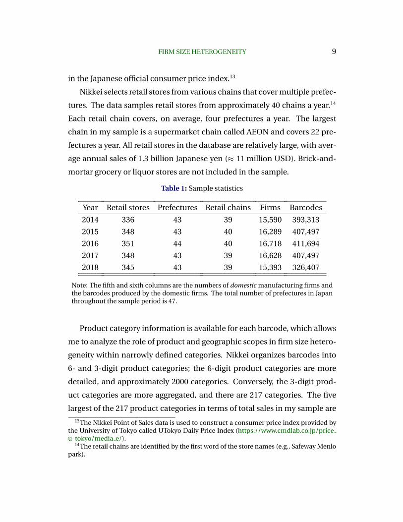
I use the Nikkei POS data from 2014 to 2018. Table 1 presents the num-

ber of retail stores, retail chains, prefectures, manufacturing firms, and bar-

codes in the sample. The data covers on average 350 retail stores a year.

These stores represent a geographically balanced sample of 43 out of 47 pre-

fectures located in Japan. The sales volume in each prefecture in the data is

correlated with the actual market size of the prefecture.12 For example, the

three largest prefectures in terms of their populations (Tokyo, Osaka, and

Kanagawa) are the three largest prefectures in terms of the number of stores

and sales in the sample.

I observe the wide range of goods purchased by consumers at retail stores

in the data. The database covers approximately 420 billion Japanese yen (≈ 4

billion USD) worth of transactions and 400, 000 barcodes spanning across

16, 000 manufacturing firms per year. Because Nikkei mainly samples super-

markets and convenience stores, the products in the data comprise mostly

consumer packaged goods, such as processed foods, beverages, and house-

hold goods. Overall, the data covers around 20% of all expenditure on goods

12The market size of each prefecture can be measured by prefecture-level employment(https://www.stat.go.jp/data/roudou/pref/index.html) or GDP (https://www.esri.cao.go.jp/jp/sna/data/data list/kenmin/files/files kenmin.html). Both measures show a positivecorrelation with the prefecture sale volume in the Nikkei POS from 2014 to 2018.

FIRM SIZE HETEROGENEITY 9

in the Japanese official consumer price index.13

Nikkei selects retail stores from various chains that cover multiple prefec-

tures. The data samples retail stores from approximately 40 chains a year.14

Each retail chain covers, on average, four prefectures a year. The largest

chain in my sample is a supermarket chain called AEON and covers 22 pre-

fectures a year. All retail stores in the database are relatively large, with aver-

age annual sales of 1.3 billion Japanese yen (≈ 11 million USD). Brick-and-

mortar grocery or liquor stores are not included in the sample.

Table 1: Sample statistics

Year Retail stores Prefectures Retail chains Firms Barcodes

2014 336 43 39 15,590 393,313

2015 348 43 40 16,289 407,497

2016 351 44 40 16,718 411,694

2017 348 43 39 16,628 407,497

2018 345 43 39 15,393 326,407

Note: The fifth and sixth columns are the numbers of domestic manufacturing firms andthe barcodes produced by the domestic firms. The total number of prefectures in Japanthroughout the sample period is 47.

Product category information is available for each barcode, which allows

me to analyze the role of product and geographic scopes in firm size hetero-

geneity within narrowly defined categories. Nikkei organizes barcodes into

6- and 3-digit product categories; the 6-digit product categories are more

detailed, and approximately 2000 categories. Conversely, the 3-digit prod-

uct categories are more aggregated, and there are 217 categories. The five

largest of the 217 product categories in terms of total sales in my sample are

13The Nikkei Point of Sales data is used to construct a consumer price index provided bythe University of Tokyo called UTokyo Daily Price Index (https://www.cmdlab.co.jp/priceu-tokyo/media e/).

14The retail chains are identified by the first word of the store names (e.g., Safeway Menlopark).

10 YOKO SHIBUYA

Bento (packaged meal in a box for take-out), rice, frozen food, yogurt, and

pastry. The 6- or 3-digit product categories are used to generate the below

empirical facts depending on the appropriate level of aggregation.

Firm size, product and geographic scopes

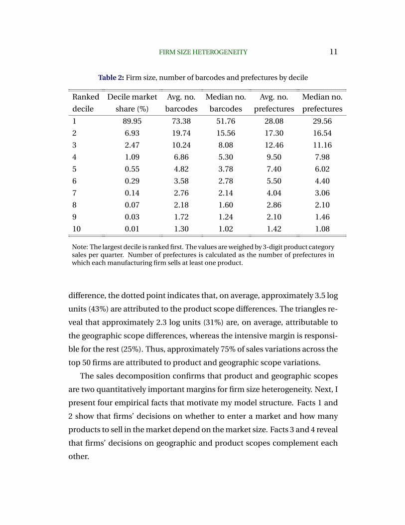
Table 2 presents the market share, product scope, and geographic scope by

ranked decile in the sample. I calculate the decile values for each quarter

and 3-digit product category and weigh the values by the product category-

quarter sales. Three striking features emerge. First, the markets are skewed

toward a few large firms — the largest 10% of firms occupy approximately

90% of the market share. Second, larger firms sell more products than smaller

firms — the largest 10% of firms sell 77 barcodes, while the median firms sell

four barcodes. Finally, larger firms sell their products in more locations —

the largest 10% of firms sell their products in 28 out of 43 prefectures, while

the median firms sell in six.15

How important are product and geographic scopes, compared with in-

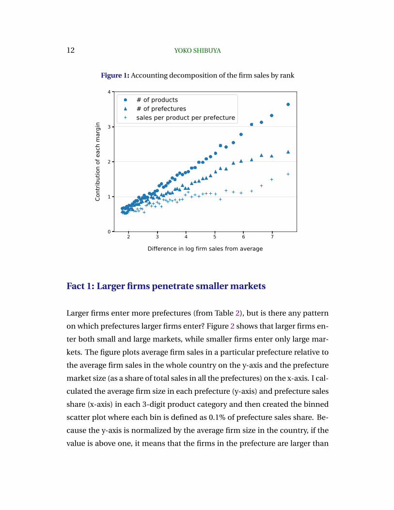
tensive margin, to account for the observed firm size distribution? Figure 1

presents an accounting decomposition of the firm sales into the number

of products firms sell (product scope), the number of prefectures in which

firms sell their products (geographic scope), and the sales per product per

prefecture (intensive margin) for the 50 firms with the largest average mar-

ket share in each product category. Each point represents an average con-

tribution of a particular margin. For example, the column of points at the

right of the figure indicates that the largest firm in a product group is, on av-

erage, almost eight log units larger than an average firm. Of this 8 log unit

15A common concern regarding product scope is that larger firms might be connectedone large retail chain and sell their products in many stores and prefectures within thechain. As shown in Section A.1, this is not the case: larger firms sell in more retail chains,and these retail chains are not systematically larger than the retail chains that smaller firmssell their products in.

FIRM SIZE HETEROGENEITY 11

Table 2: Firm size, number of barcodes and prefectures by decile

Ranked

decile

Decile market

share (%)

Avg. no.

barcodes

Median no.

barcodes

Avg. no.

prefectures

Median no.

prefectures

1 89.95 73.38 51.76 28.08 29.56

2 6.93 19.74 15.56 17.30 16.54

3 2.47 10.24 8.08 12.46 11.16

4 1.09 6.86 5.30 9.50 7.98

5 0.55 4.82 3.78 7.40 6.02

6 0.29 3.58 2.78 5.50 4.40

7 0.14 2.76 2.14 4.04 3.06

8 0.07 2.18 1.60 2.86 2.10

9 0.03 1.72 1.24 2.10 1.46

10 0.01 1.30 1.02 1.42 1.08

Note: The largest decile is ranked first. The values are weighed by 3-digit product categorysales per quarter. Number of prefectures is calculated as the number of prefectures inwhich each manufacturing firm sells at least one product.

difference, the dotted point indicates that, on average, approximately 3.5 log

units (43%) are attributed to the product scope differences. The triangles re-

veal that approximately 2.3 log units (31%) are, on average, attributable to

the geographic scope differences, whereas the intensive margin is responsi-

ble for the rest (25%). Thus, approximately 75% of sales variations across the

top 50 firms are attributed to product and geographic scope variations.

The sales decomposition confirms that product and geographic scopes

are two quantitatively important margins for firm size heterogeneity. Next, I

present four empirical facts that motivate my model structure. Facts 1 and

2 show that firms’ decisions on whether to enter a market and how many

products to sell in the market depend on the market size. Facts 3 and 4 reveal

that firms’ decisions on geographic and product scopes complement each

other.

12 YOKO SHIBUYA

Figure 1: Accounting decomposition of the firm sales by rank

2 3 4 5 6 7

Difference in log firm sales from average

0

1

2

3

4Co

ntrib

utio

n of

eac

h m

argi

n# of products# of prefecturessales per product per prefecture

Fact 1: Larger firms penetrate smaller markets

Larger firms enter more prefectures (from Table 2), but is there any pattern

on which prefectures larger firms enter? Figure 2 shows that larger firms en-

ter both small and large markets, while smaller firms enter only large mar-

kets. The figure plots average firm sales in a particular prefecture relative to

the average firm sales in the whole country on the y-axis and the prefecture

market size (as a share of total sales in all the prefectures) on the x-axis. I cal-

culated the average firm size in each prefecture (y-axis) and prefecture sales

share (x-axis) in each 3-digit product category and then created the binned

scatter plot where each bin is defined as 0.1% of prefecture sales share. Be-

cause the y-axis is normalized by the average firm size in the country, if the

value is above one, it means that the firms in the prefecture are larger than

FIRM SIZE HETEROGENEITY 13

the average firms in the country.16 The negative slope in the figure indicates

that larger firms are more likely to penetrate smaller prefectures.

Figure 2: Average firm size in each prefecture

0.0 2.5 5.0 7.5 10.0 12.5 15.0

Prefecture sales share (%)

0.80

0.85

0.90

0.95

1.00

1.05

1.10

Aver

age

firm

size

in e

ach

pref

ectu

re

(rel

ativ

e to

the

aver

age

in th

e ec

onom

y)

Average firm sales in the economy

Fact 2: Firms sell more products in larger markets

How do firms’ decisions on how many products to sell in a market depend

on the market size? Figure 3 shows that the number of products firms sell

increases with the market size. The figure plots firms’ number of products

in each prefecture (relative to the average number of products of the same

firm across prefectures) on the y-axis and prefecture market size (as a share

of total sales in all the prefectures) on the x-axis. I calculated the average

number of products of firms in each prefecture (y-axis) and prefecture sales

16For example, the point on the left end shows that the average firm size in the prefecturesthat have 0.0 to 0.1% of prefecture sales shares is 1.12 times larger than the average firm sizein the economy.

14 YOKO SHIBUYA

share (x-axis) in each 3-digit product category and created the binned scat-

ter plot, where each bin is defined as 0.1% of prefecture sales share.17 The

positive slope in the figure suggests that the same firms sell more products

in larger markets.

Figure 3: Firm’s number of products in each prefecture

0.0 2.5 5.0 7.5 10.0 12.5 15.0

Prefecture sales share (%)

0.6

0.7

0.8

0.9

1.0

1.1

1.2

1.3

Firm

's nu

mbe

r of p

rodu

cts i

n ea

ch p

refe

ctur

e (r

elat

ive

to th

e av

erag

e of

the

sam

e fir

m in

the

econ

omy)

Average number of products of the same firm

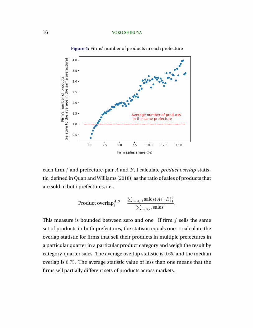
Fact 3: Larger firms sell more products in a given market

According to Figure 4, larger firms not only sell more products in the econ-

omy (see Table 2), but they also sell more products in each particular mar-

ket. The figure plots firms’ number of products in each prefecture on the

y-axis and the firm sales share on the x-axis. The y-axis is normalized by the

average number of products per firm in the same prefecture. I calculated

17For example, the figure suggests that if firms sell their products in prefectures that have2.5% and 5% of sales shares, then the same firms sell 10% more products in the prefecturewith 5% of sales share than in the prefecture with 2.5% of sales share.

FIRM SIZE HETEROGENEITY 15

firms’ number of products in each prefecture relative to the average num-

ber of products per firm in the same prefecture (y-axis) and firm sales share

(x-axis) in each 3-digit product category and created the binned scatter plot

where each bin is defined as 0.1% of firm sales share.18 The positive slope

indicates that the firms with a larger sales share in the economy sell more

products in each market.

Fact 3 implies that firms’ choices on product and geographic scopes are

interconnected. As firms expect to sell more products and generate larger

profits in a market, they are more likely to enter the market.19 Therefore, a

larger product scope generates a wider geographic scope.

Fact 4: Firms adjust varieties to heterogeneous local taste

Fact 4 suggests another complementarity between geographic and product

scopes. First, I show that firms sell (partially) different sets of products across

markets. Second, I present the evidence of consumer taste heterogeneity

across markets. The evidence is consistent with the story that firms offer

different varieties across markets to cater to heterogeneous consumer tastes.

Fact 4-1: Firms sell different sets of products across markets

Do firms sell the same sets of products in all the markets they operate in? Or

do they sell different sets of products across markets? To answer the ques-

tion, I measure the similarity of firms’ product sets across prefectures. For

18For example, the figure suggests that firms with 2.5% of sales share in the economy sellsabout 50% more products than the average firms in the same prefecture in the prefecturesthat the firm sells their products in.

19One caveat of this argument that firms with more products might sell less per productand thus, these firms do not expect larger profits. However, as confirmed in Figure 1, firms’number of product and sales per product are positively correlated. Therefore, when firmsexpect to sell more products in a market, they will expect to generate larger profits in themarket.

16 YOKO SHIBUYA

Figure 4: Firms’ number of products in each prefecture

0.0 2.5 5.0 7.5 10.0 12.5 15.0

Firm sales share (%)

0.5

1.0

1.5

2.0

2.5

3.0

3.5

4.0Fi

rm's

num

ber o

f pro

duct

s(re

lativ

e to

the

aver

age

in th

e sa

me

pref

ectu

re)

Average number of products in the same prefecture

each firm f and prefecture-pair A and B, I calculate product overlap statis-

tic, defined in Quan and Williams (2018), as the ratio of sales of products that

are sold in both prefectures, i.e.,

Product overlapA,Bf =

∑i=A,B sales(A ∩B)if∑

i=A,B salesi.

This measure is bounded between zero and one. If firm f sells the same

set of products in both prefectures, the statistic equals one. I calculate the

overlap statistic for firms that sell their products in multiple prefectures in

a particular quarter in a particular product category and weigh the result by

category-quarter sales. The average overlap statistic is 0.65, and the median

overlap is 0.75. The average statistic value of less than one means that the

firms sell partially different sets of products across markets.

FIRM SIZE HETEROGENEITY 17

Fact 4-2: Consumer tastes are heterogeneous across prefectures

The most likely reason for the incomplete product overlap is that firms offer

different sets of products across prefectures to cater to heterogeneous lo-

cal taste.20,21 To see whether consumer taste is indeed heterogeneous across

prefectures in Japan, I calculated the variations of market share of the same

products across different prefectures.

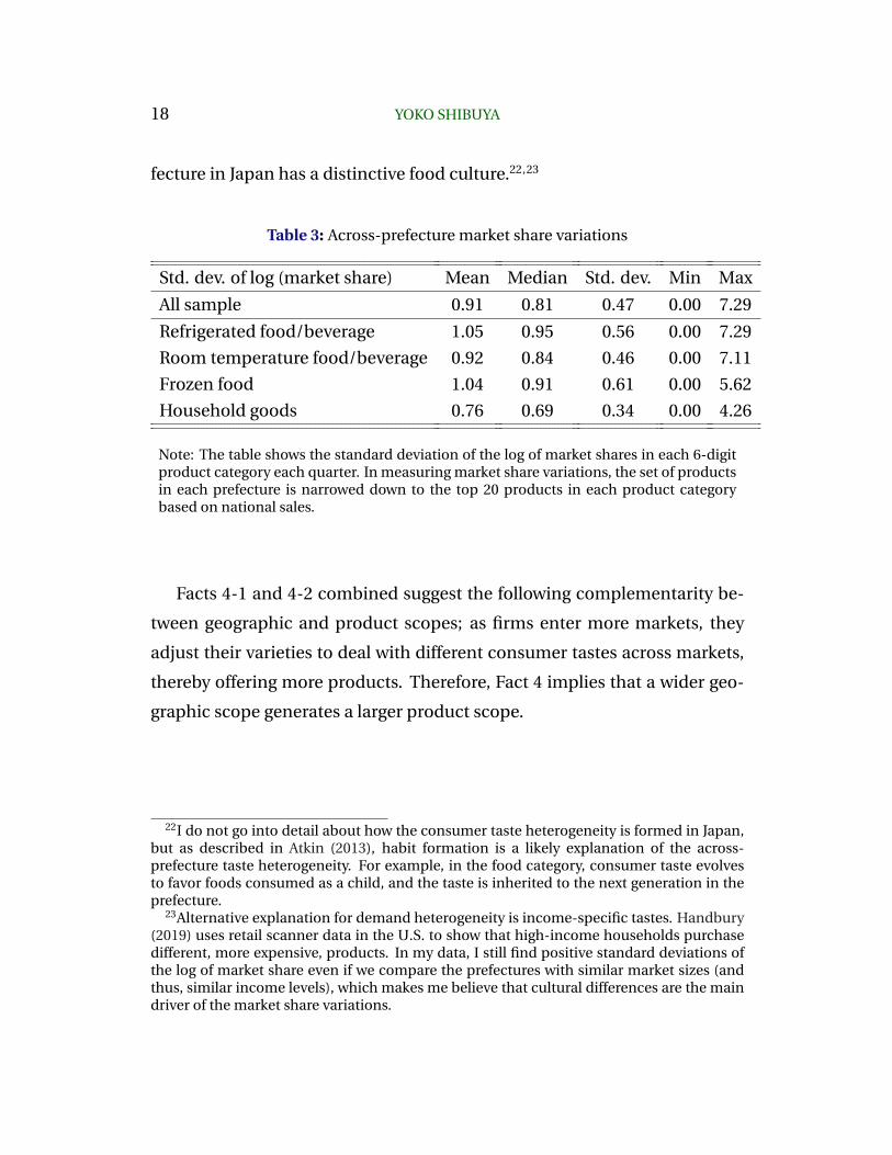
The data suggest that the taste across the prefectures is indeed heteroge-

neous. The first row of Table 3 presents the standard deviation of the log of

market share of the top 20 products ranked by national sales in each 9-digit

product category. If consumer tastes were homogeneous across prefectures,

the share of sales accruing to these products would be expected to be the

same in any prefectures; therefore the standard deviations are close to zero.

The mean and median standard deviations of the log of market share in all

samples are 0.91 and 0.81, respectively. Positive standard deviations indicate

the existence of across-prefecture taste heterogeneity in Japan.

The second to fifth rows of Table 3 show the standard deviations of the

log of market share for refrigerated, room temperature and frozen foods,

and household goods, respectively. Food categories have larger market share

variations across prefectures than household goods, reflecting that each pre-

20There is extensive literature that contains empirical evidence on across-market tasteheterogeneity in the industrial organization field (for example, Waldfogel (2003), Waldfogelet al. (2004), Bronnenberg et al. (2009), Choi and Bell (2011), and Bronnenberg et al. (2012))Furthermore, Waldfogel (2008) and Quan and Williams (2018) document the evidence ofsupply-side response to the across-market consumer taste heterogeneity.

21I acknowledge that there may be some supply-side factors that affect product overlapbetween prefectures, such as shipping costs. However, the products covered in the data areconsumer packaged goods, and shipping costs of these products are usually small. Frozenfoods involve relatively higher shipping costs within consumer packaged goods, but theyoccupy only less than 3% of overall sales in my sample.

18 YOKO SHIBUYA

fecture in Japan has a distinctive food culture.22,23

Table 3: Across-prefecture market share variations

Std. dev. of log (market share) Mean Median Std. dev. Min Max

All sample 0.91 0.81 0.47 0.00 7.29

Refrigerated food/beverage 1.05 0.95 0.56 0.00 7.29

Room temperature food/beverage 0.92 0.84 0.46 0.00 7.11

Frozen food 1.04 0.91 0.61 0.00 5.62

Household goods 0.76 0.69 0.34 0.00 4.26

Note: The table shows the standard deviation of the log of market shares in each 6-digitproduct category each quarter. In measuring market share variations, the set of productsin each prefecture is narrowed down to the top 20 products in each product categorybased on national sales.

Facts 4-1 and 4-2 combined suggest the following complementarity be-

tween geographic and product scopes; as firms enter more markets, they

adjust their varieties to deal with different consumer tastes across markets,

thereby offering more products. Therefore, Fact 4 implies that a wider geo-

graphic scope generates a larger product scope.

22I do not go into detail about how the consumer taste heterogeneity is formed in Japan,but as described in Atkin (2013), habit formation is a likely explanation of the across-prefecture taste heterogeneity. For example, in the food category, consumer taste evolvesto favor foods consumed as a child, and the taste is inherited to the next generation in theprefecture.

23Alternative explanation for demand heterogeneity is income-specific tastes. Handbury(2019) uses retail scanner data in the U.S. to show that high-income households purchasedifferent, more expensive, products. In my data, I still find positive standard deviations ofthe log of market share even if we compare the prefectures with similar market sizes (andthus, similar income levels), which makes me believe that cultural differences are the maindriver of the market share variations.

FIRM SIZE HETEROGENEITY 19

3. Survey of Japanese food manufacturing firms

Next, I conduct a survey of Japanese food manufacturing firms to help me

determine a modeling structure. The literature proposes various model struc-

tures that generate the product or geographic variations across firms. The

survey results suggest that, among these candidate model structures, two

types of fixed costs are of practical importance: the fixed cost of entering a

market and the fixed cost of selling a product.

3.1 Survey background and goal

Two candidate structures generate product scope variations across firms:

the fixed cost of selling a product and the cost of investment into production

capital. The fixed cost of selling a product is usually interpreted as the cost

of marketing research or product development/customization (Hottman et

al., 2016). The cost of investment into production capital manifests as the

so-called flexible manufacturing allowing a firm to add another variety to

the existing product line but with an increase in the marginal cost for the

new products (Eckel and Neary, 2010). The difference between the two costs

is that investment cost increases as the firm adds more products, whereas

the fixed cost of selling a product does not depend on the firm’s number of

products.

Similarly, the literature proposes two candidate model elements for geo-

graphic scope variations across firms: the fixed cost of entering a market and

the marketing cost. The fixed cost of entering a market is frequently used in

many international trade papers and takes the form of the fixed cost of ex-

porting (Melitz, 2003). Meanwhile, the marketing cost generates geographic

scope variations in asymmetric information settings. When consumers do

not know what products are available, firms incur marketing costs to in-

20 YOKO SHIBUYA

crease their consumer base (Arkolakis, 2010). The difference between the

two costs is due to the fact that the marketing cost to reach additional con-

sumer decreases with the market size, while the fixed cost of entering a mar-

ket does not depend on the market size.

Instead of making an arbitrary choice from candidate model structures,

I surveyed Japanese packaged food manufacturing firms to find out which

model structures are of the most practical relevance. The survey took place

in one of the biggest food supplier-buyer matching events in Japan, called

Food Selection 2020 (the survey and matching event are described in detail

in Appendix A). The event gathers packaged food manufacturing firms (sup-

pliers) from all over Japan. The suppliers show their latest products and try

to make sales contracts with buyers, while the buyers, ranging from whole-

sale and retail to restaurants, try to find new products to purchase in the

event.

Before conducting the survey, I observed 50 supplier-buyer negotiations

in the matching event to find counterparts of these four model elements

(fixed cost of entering a market and selling a product, marketing cost, and

investment cost) in the business world. The marketing cost and the cost of

investment into production capital have direct counterparts in the business

world: the advertisement cost to increase consumer awareness and the cost

of investment into factories. The fixed cost of entering a market corresponds

to the cost of overcoming contract issues with buyers. In the supplier-buyer

negotiations, buyers frequently ask suppliers to use the same logistic com-

pany as the buyer, open a new bank account specific to the contract, and

go through other administrative processes related to the contract.24 Lastly,

the fixed cost of selling a product in a market corresponds to the cost of

consumer market research and customizing each product to cater to con-

24The quantitative importance of the fixed cost of overcoming contract friction on welfaregains from trade in the international trade context is documented by Startz (2016).

FIRM SIZE HETEROGENEITY 21

sumers’ tastes. In the negotiations, buyers often ask suppliers to customize

their products to match the consumers’ tastes in the buyers’ areas.

3.2 Survey results

Based on the observations in 50 supplier-buyer negotiations, I asked the

suppliers about the relative importance of the four cost counterparts in their

businesses. Specifically, I asked: How important are the following elements

in expanding into new geographic markets and increasing product range?

(1) Overcoming contracting issues with the buyers, (2) understanding con-

sumers’ tastes and customizing products to cater to the tastes, (3) having

sufficient production capacity for the new market, and (4) advertising prod-

ucts to increase consumer awareness.

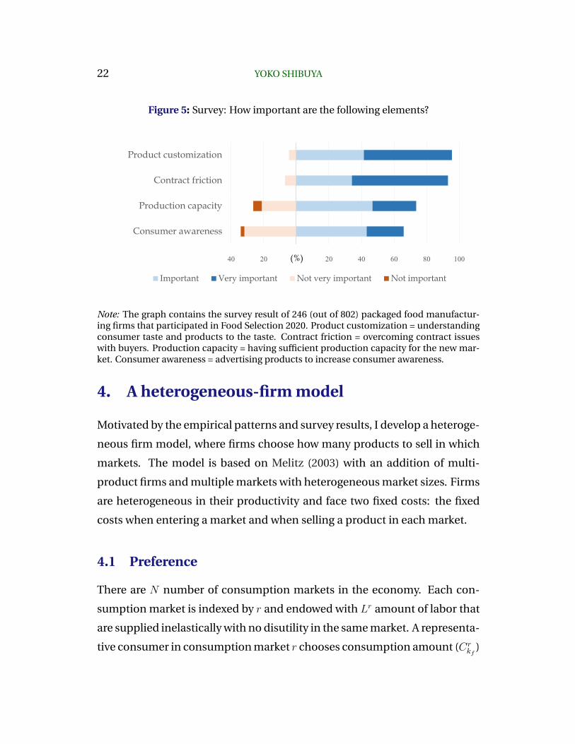
Figure 5 shows the survey results. The surveyed firms think that product

customization and overcoming contracting issues with buyers are of equal

and practical importance. Having sufficient production capacity and in-

creasing consumer awareness turn out to be less important. The cost of con-

tracting with a buyer corresponds to the fixed cost of entering a market, and

the cost of understanding consumer tastes and customizing products corre-

sponds to the fixed costs of selling a product in each market. Therefore, the

results imply that the two fixed costs have more practical importance than

the other two candidate structures.

It should be noted that the survey results are specific to the firms in the

Japanese packaged food manufacturing industry, and different contexts would

generate different insights for the model structures. For example, increasing

consumer awareness can be more important in other sectors such as tech-

nology, service, and healthcare (see Hulcr et al., 2019).

22 YOKO SHIBUYA

Figure 5: Survey: How important are the following elements?

40 20 20 40 60 80 100

Consumer awareness

Production capacity

Contract friction

Product customization

Important Very important Not very important Not important

(%)

Note: The graph contains the survey result of 246 (out of 802) packaged food manufactur-ing firms that participated in Food Selection 2020. Product customization = understandingconsumer taste and products to the taste. Contract friction = overcoming contract issueswith buyers. Production capacity = having sufficient production capacity for the new mar-ket. Consumer awareness = advertising products to increase consumer awareness.

4. A heterogeneous-firm model

Motivated by the empirical patterns and survey results, I develop a heteroge-

neous firm model, where firms choose how many products to sell in which

markets. The model is based on Melitz (2003) with an addition of multi-

product firms and multiple markets with heterogeneous market sizes. Firms

are heterogeneous in their productivity and face two fixed costs: the fixed

costs when entering a market and when selling a product in each market.

4.1 Preference

There are N number of consumption markets in the economy. Each con-

sumption market is indexed by r and endowed with Lr amount of labor that

are supplied inelastically with no disutility in the same market. A representa-

tive consumer in consumption market r chooses consumption amount (Crkf

)

FIRM SIZE HETEROGENEITY 23

of each product kf sold by firm f to maximize the following constant elastic-

ity of substitution (CES) utility function subject to the budget constraint:

U r =

[∫f∈Ωr

∫kf∈Ωrf

(φrkfC

rkf

)σ−1σ

dkf df

] σσ−1

, (1)

where Ωr is the endogenous set of firms selling in consumption market r, Ωrf

is the endogenous set of products that firm f sells in consumption market r,

and prkf and φrkf are the price and taste shifter of product kf in consumption

market r, respectively. The parameter σ > 1 is the elasticity of substitution

across the products.

The taste shifter φrkf captures consumer taste heterogeneity across mar-

kets. The taste shifter is a product of a common component, φkf , and an

i.i.d. regional shock to the common component, εrkf , i.e., φrkf = φkf × εrkf .

The common component captures a taste for a product that is common

across all markets and is drawn from a log-normal distribution with mean

µ and variance σ2: log φkf ∼ N(µ, σ2). The regional shock captures an id-

iosyncratic taste difference across markets and is drawn for each product

and market from a log-normal distribution with mean 0 and variance σ2ε :

log εrkf ∼ N(0, σ2ε ).25 Because a product of two log-normally distributed ran-

dom variables follows a log-normal distribution, the taste shifter also fol-

lows log-normal distribution with mean µ and variance σ2 + σ2ε : log φrkf ∼

N(µ, σ2 + σ2ε ).26

25This taste heterogeneity can also be thought as taste differences coming from wealth-iness of the prefectures, i.e., households in wealthy prefectures prefer different productsfrom households in poor prefectures. However, this model does not capture the possibilitythat households in wealthier cities prefer more expensive products.

26Using a log-normal distribution for consumer tastes has an advantage in fitting the data.With the consumer tastes following log-normal and productivity following Pareto distribu-tions, sales per product per region increases with productivity, which fits the empirical find-ing in the Japanese data (see Figure 1). This is in contrast with assuming Pareto distributionfor consumer tastes and productivity, where sales per product per region becomes indepen-dent of productivity. See Fernandes et al. (2019) for more discussion.

24 YOKO SHIBUYA

The corresponding price index for the consumption market r is given by

P r ≡

∫f∈Ωr

∫kf∈Ωrf

(prkfφrkf

)1−σ

dkf df

11−σ

. (2)

4.2 Technology and market structure

There is an unbounded measure of potential firms who are identical prior to

their entry into the economy. To enter, firms must incur a fixed cost of en-

tering the economy, Fe in units of labor. Once the fixed cost is incurred, each

firm f draws productivity ϕf from a Pareto distribution with a shape param-

eter θ and a scale parameter ϕ: ϕf ∼ Pareto(θ, ϕ). Similarly, once the fixed

cost of entering the economy is incurred, each firm observes a common and

a regional shock component of taste shifter for each potential product kf in

consumption market r.27 Each firm is endowed with mass K of potential

products. The mass of potential products is constant across firms, but the

sets of potential products are differentiated across firms. Among the sets of

potential products, each firm chooses which products to sell in a particular

market.

Once the fixed cost of entering the economy has been incurred, and firm’s

productivity and taste shifter have been observed, the firm decides whether

to enter each market and which products to sell in each market. Upon choos-

ing which products to sell in which markets, firms face two types of fixed

costs. When a firm enters a consumption market (i.e., sells at least one prod-

uct in a consumption market), the firm pays the fixed cost of entering a mar-

ket, F . In addition, firms incur the fixed cost of selling per product in a given

27To exploit the low of large numbers’ feature, it is assumed that the productivity, com-mon component, and regional shock components are independent of one another and in-dependently distributed across firms. Similarly, it is assumed that the common componentis independently distributed across the products, while the regional shock component isindependently distributed across products and consumption markets.

FIRM SIZE HETEROGENEITY 25

market, Fp.28 Two types of fixed costs are paid in units of labor.

In addition to the fixed costs, there is also a marginal cost of producing

each product. The marginal cost of selling a product is the same across prod-

ucts and markets within a firm due to the following assumptions. First, the

production function is the same across products and firms and is linear in

labor, the sole factor of production. The total amount of labor needed to

produce one unit of output is 1ϕf

. Second, I assume the free mobility of firms

in the economy. The representative consumers supply Lr unit of labor in

consumption market r, and if there are any wage differences across markets,

firms keep moving until the wages are equalized. Therefore, there is only a

single wage in the economy.29 A single wage in the economy is defined as w

and normalized as one. Third, I assume there are no variable costs of trade

across markets. In total, firm f ’s marginal cost of selling a product is given

by wϕ−1f = ϕ−1

f , where the equality comes from the normalization of w = 1.

This leads to an observation that the marginal cost is common across prod-

ucts and markets within a firm.

Each consumption market is monopolistically competitive. With the CES

utility function specified in (1), firms’ pricing decision is given by constant

markup times the marginal cost:

prkf =σ

σ − 1ϕ−1f , (3)

where the pricing is common across products and markets within a firm.

28For example, when a firm enters one market and sells two products there, it paysF+2Fp

amount of fixed costs.29A free mobility of firms across markets can be interpreted as a free mobility of workers,

which also equates wages across markets and generates a single wage in the economy.

26 YOKO SHIBUYA

4.3 Firms’ decisions on which products to sell where

Firms’ profit maximization problem is separable across consumption mar-

kets. In each consumption market r, firms decide which products to sell

in the market and whether to enter the market with the following two steps:

First, given entering a market, firms choose an optimal set of products to sell

in the market. Next, given the optimal set of products, firms decide whether

to enter the market. The first step generates a cutoff taste shifter condition,

and the second step generates a cutoff productivity condition.

The cutoff taste shifter condition. Using the pricing rule defined by ex-

pression (3), the equilibrium revenue received by a firm f in consumption

market r from selling a product kf is:

r(ϕf , φrkf

) =

(σ

σ − 1

)1−σ

(φrkfϕfPr)σ−1Lr. (4)

The corresponding equilibrium profits from selling the product to that mar-

ket are:

π(ϕf , φrkf

) =r(ϕf , φ

rkf

)

σ− Fp. (5)

Firm f sells product kf if and only if the profit from selling the product is

positive, i.e., π(ϕf , φrkf

) > 0. Because the demand for a product is monoton-

ically increasing in the taste shifter, and r(ϕf ,∞σ

> Fp and r(ϕf ,0)

σ< Fp hold for

any given productivity level ϕf , a cutoff taste shifter for each firm f in market

r, φr∗f , is defined as

π(ϕf , φr∗f ) = 0. (6)

Condition (6) is called a cutoff taste shifter condition. Given entering a mar-

ket, firm f sells products with a taste shifter higher than the cutoff value, φr∗f .

FIRM SIZE HETEROGENEITY 27

The cutoff productivity condition. Given the optimal set of products de-

fined as a set of products with a taste shifter above the cutoff taste shifter,

the firm chooses whether to enter the consumption market. Firm f ’s profit

in consumption market r is given by

Πr(ϕf ) =

∫kf∈Ωrf

π(ϕf , φr∗f ) dkf − F. (7)

The first term in (7) is the variable profit from selling the optimal set of prod-

ucts Ωrf (chosen by the cutoff taste shifter condition (6)), and the last term

reflects the fixed cost of entering the market.

Each firm f enters consumption market r if and only if entering a market

generates a positive profit, i.e., Πr(ϕf ) > 0. Because the demand for products

is monotonically increasing with productivity of the firm, and Πr(∞) > 0 and

Πr(0) < 0 hold for any market r, the cutoff productivity in each market r, ϕr∗,

is defined as

Πr(ϕr∗) = 0. (8)

This condition is called the cutoff productivity condition. Firms with pro-

ductivity higher than the cutoff productivity enter the market.

4.4 Free-entry

The mass of firms in the economy, M , is determined by a free-entry condi-

tion. The free-entry condition ensures that firms keep entering the economy

until the expected profit of entering the economy becomes equal to zero, i.e.,

ΣrΠr

M= Fe,

where Πr ≡∫f∈Ωr

Πr(ϕf ) df is the sum of profits of all surviving firms in the

consumption market r.

28 YOKO SHIBUYA

Among the firms entering the economy, firms with productivity above

the cutoff productivity ϕr∗ enter the consumption market r. Define G(ϕf ) as

the cumulative distribution function of the Pareto distribution for produc-

tivity. Then, the mass of firms entering each market r, M r, is given by

M r = M(1−G(ϕr∗)).

4.5 Aggregation

Using the cutoff taste shifter condition for each firm (6), the cutoff produc-

tivity condition (8), and the pricing strategy for each firm (3), the price index

in the consumption market r (2) can be rewritten as

P r =

[M

∫ ∞ϕr∗

p(ϕf )1−σK

∫ ∞φr∗f

(φrkf )σ−1dF (φrkf )dG(ϕf )

] 11−σ

, (9)

where F (φrkf ) is a cumulative distribution function of taste shifter.

For a given number of firms in the market, a decrease in the cutoff taste

shifter for each firm affects the price index in two ways. First, a lower cut-

off taste shifter means each firm sells more products, which decreases the

price index because of the love-of-variety effect. Second, it lowers the av-

erage taste shifter for each firm as more marginal products are introduced

to the market, and a lower average taste shifter, in turn, increases the price

index.

Similarly, for a given number of products for each firm, a decrease in the

cutoff productivity in each market has two effects on the price index. On the

one hand, it decreases the price index due to the love of variety effect. On

the other hand, it increases the price index because the average productivity

decreases as more marginal firms enter the market. These insights will be

dealt with further when discussing the efficiency of the market equilibrium

FIRM SIZE HETEROGENEITY 29

in section 7.

5. Estimation and model evaluation

I structurally estimate model parameters by the simulated method of mo-

ments using the Nikkei POS data. With the quantified model, I evaluate

model performance by checking whether the model fits (1) four empirical

patterns found in Section 2, and (2) the firm size, product scope, and geo-

graphic scope distributions observed in the data.

5.1 Structural estimation

First, I explain the identification issues in estimating productivity (ϕf ) and

the constant elasticity of substitution (σ). Second, I explain how I simulate

a set of firms given a particular set of parameter values and how I use the

simulated method of moments (SMM) to overcome the identification issue.

Finally, I describe the simulation algorithm.

The model parameters are divided into four categories. The first category

is the parameters that can be directly determined by the data. The number

of markets (R) and the labor endowment of each market (Lr) are included

in this category. The second category comprises the parameters that are es-

timated given from the data. The parameters for taste shifter distributions

log(φk) ∼ N(µ, σ2), log(εrk) ∼ N(0, σ2ε ) are included in this category. The

third category is the parameters that are estimated to match some moments

in the data. The mass of potential products for each firm (K) is set so that

the lowest-productivity firm produces at least one product. There are three

types of fixed costs F, Fp, Fe set to match the top 10% vs. median firms’

stats of firm size, product, and geographic scopes. Specifically, compared to

the median firms, the top 10% firms generates 188 times more sales, pro-

30 YOKO SHIBUYA

duce 18.8 times more products, and enter 4.8 times more markets, and the

three fixed costs are set to match the three targeted values. The final category

is the parameters that are estimated using SMM to deal with identification

issues. The elasticity of substitution (σ) and parameters for productivity dis-

tribution ϕf ∼ Pareto(θ, ϕ) are in this category. I define Θ1 = F, Fp, Fe as

a set of parameters that are estimated using GMM, and Θ2 = σ, (θ, ϕ) as a

set of parameters that are estimated using SMM.

5.1.1 Identification issues

First, it is necessary to explain how it is possible to potentially estimate the

values of the elasticity of substitution (σ) from the firm-level expenditure

shares and prices. Define firm f ’s expenditure share in the consumption

market r as Srf and the number of products firm f produces in market r as

N rf . Then, firm f ’s expenditure share per product in market r is given by

logSrfN rf

= (1− σ) log prf + (σ − 1) logP r +1

N rf

∫kf∈Ωr∗f

(φrk,f )σ−1dkf , (10)

It is possible to estimate σ from using equation (10), i.e., by regressing the

firm sales share per product on firm price and market fixed effect.30 How-

ever, such an estimation suffers from selection bias. The assumption re-

quired for the identification is firm prices and the average taste shifter are

orthogonal, i.e., prf ⊥ 1Nrf

∫kf∈Ωr∗f

(φrk,f )σ−1dkf , which is likely to be violated.

Firms with a higher productivity (and thus a lower price) can sell products

with a lower taste shifter, which leads to a positive correlation between firms’

prices and the average taste shifter, underestimating σ.

The estimation of productivity (ϕf ) suffers from a similar selection bias.

Productivity can be estimated from the data on the product-level expendi-

30Upon estimating σ, I compute firm-level price as the average of product-level prices ineach market weighted by expenditure share of each product within firm.

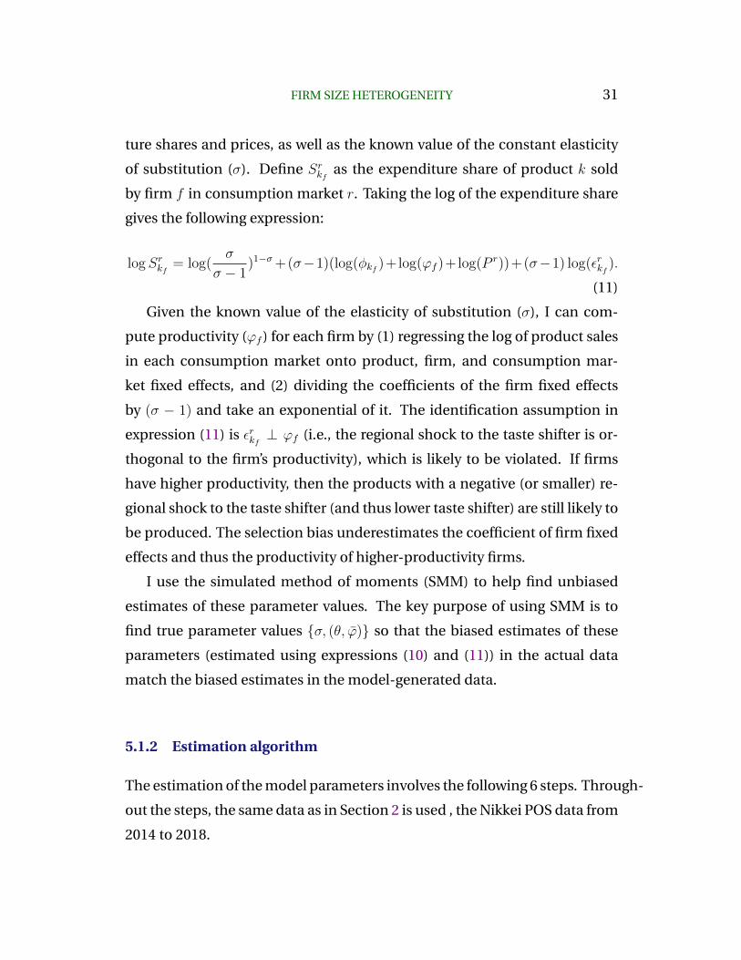
FIRM SIZE HETEROGENEITY 31

ture shares and prices, as well as the known value of the constant elasticity

of substitution (σ). Define Srkf as the expenditure share of product k sold

by firm f in consumption market r. Taking the log of the expenditure share

gives the following expression:

logSrkf = log(σ

σ − 1)1−σ+(σ−1)(log(φkf )+log(ϕf )+log(P r))+(σ−1) log(εrkf ).

(11)

Given the known value of the elasticity of substitution (σ), I can com-

pute productivity (ϕf ) for each firm by (1) regressing the log of product sales

in each consumption market onto product, firm, and consumption mar-

ket fixed effects, and (2) dividing the coefficients of the firm fixed effects

by (σ − 1) and take an exponential of it. The identification assumption in

expression (11) is εrkf ⊥ ϕf (i.e., the regional shock to the taste shifter is or-

thogonal to the firm’s productivity), which is likely to be violated. If firms

have higher productivity, then the products with a negative (or smaller) re-

gional shock to the taste shifter (and thus lower taste shifter) are still likely to

be produced. The selection bias underestimates the coefficient of firm fixed

effects and thus the productivity of higher-productivity firms.

I use the simulated method of moments (SMM) to help find unbiased

estimates of these parameter values. The key purpose of using SMM is to

find true parameter values σ, (θ, ϕ) so that the biased estimates of these

parameters (estimated using expressions (10) and (11)) in the actual data

match the biased estimates in the model-generated data.

5.1.2 Estimation algorithm

The estimation of the model parameters involves the following 6 steps. Through-

out the steps, the same data as in Section 2 is used , the Nikkei POS data from

2014 to 2018.

32 YOKO SHIBUYA

Preparation. Pin down the values of the number of markets (R) and the

size of each market r (Lr) from the data. The number of market is set to

match the median number of prefectures in Nikkei POS data from 2014-

2018. The size of each market is set to match the average total sales volumes

in each prefecture in the Nikkei POS data from 2014 to 2018.

Step 1. Assume true values of elasticity (σ) and productivity distribution

ϕf ∼ Pareto(θ, ϕ) in the model.

Step 2. Given the value of σ, compute the values of taste shifter (φrk,f ). Then,

compute the parameter values of the common component distribution (log(φk) ∼N(µ, σ2)) and the regional shock distribution (log(εrk) ∼ N(0, σ2

ε )). To obtain

unique values for the taste shifter for each product k for firm f in market

r (φrk,f ) , I use the variation of sales across products within each firm. The

relative expenditure shares between two products within a firm in the same

consumption market is given by

pfCrkf

pfCrk′f

=

(φrkfφrk′f

)σ−1

. (12)

For each firm f , I choose a product that is sold in the largest number of pre-

fectures prefectures in the firm as a base product such that the taste shifter of

the product is normalized as one in all consumption markets, i.e., φrkf = 1 for

all r. I then estimate the relative taste shifter of other products using expres-

sion (12).31 Finally, I obtain the common components of taste shifter (φkf )

as the average value of taste shifter of the product across all consumption

markets and regional shocks (εrkf ) from the expression φrkf = φkf × εrkf .

31Upon estimating the taste shifter, I restrict the sample to the firms that sell multipleproducts in more than five markets(prefectures).

FIRM SIZE HETEROGENEITY 33

Step 3. Compute the equilibrium in the model given the values of σ and

productivity distribution set in Step 1 and the taste shifter distribution esti-

mated in Step 2.

Step 4. Find a set of parameter values of three fixed costs F, Fp, Fe that

matches top 10% vs. median firms’ statistics in the data. Specifically, I match

between top 10% vs. median firms’ sales, product scope (number of prod-

ucts), and geographic scope (number of markets) in the equilibrium and

data. Define m(Θ1) as a vector of the top 10% vs. median moments in the

model and m(1) as the corresponding moments in the data. Then, I seek a

set of parameter values Θ1 to minimize the distance between the moments

in the data and model using the criterion function:

Θ1 = argmin (m(1)−m(Θ1))W1(m(1)−m(Θ1))′, (13)

where W1 is the variance-covariance matrix of the error function, m(1) −m(Θ1).

Step 5. Simulate 10,000 artificial firms and compute product- and firm-

level expenditure shares in each market, firm-level prices, and the number

of products for each firm (see Appendix A.3.1 for a detailed simulation al-

gorithm). Using the model-generated data, estimate (biased) σ by expres-

sion (10) and productivity ϕf by expression (8). Then, compute the best-

fitted parameter values (θ, ϕ) for the productivity distribution. By using ex-

pressions (10) and (8), the estimations suffer from the same selection bias as

they do in the actual data.

I iterate these steps until the biased estimates of (σ, (θ, ϕ)) in the model-

generated data converges to the biased estimates of these parameter values

estimated in the actual data. The SMM selects a vector of parameter values

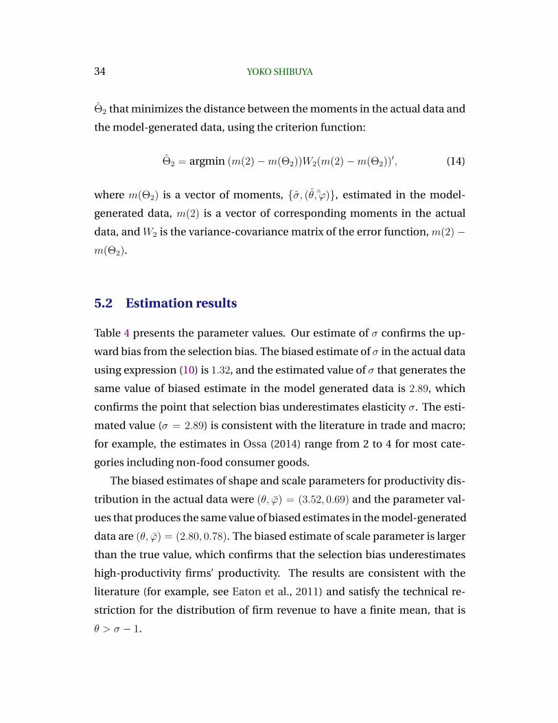
34 YOKO SHIBUYA

Θ2 that minimizes the distance between the moments in the actual data and

the model-generated data, using the criterion function:

Θ2 = argmin (m(2)−m(Θ2))W2(m(2)−m(Θ2))′, (14)

where m(Θ2) is a vector of moments, σ, (θ, ϕ), estimated in the model-

generated data, m(2) is a vector of corresponding moments in the actual

data, and W2 is the variance-covariance matrix of the error function, m(2)−m(Θ2).

5.2 Estimation results

Table 4 presents the parameter values. Our estimate of σ confirms the up-

ward bias from the selection bias. The biased estimate of σ in the actual data

using expression (10) is 1.32, and the estimated value of σ that generates the

same value of biased estimate in the model generated data is 2.89, which

confirms the point that selection bias underestimates elasticity σ. The esti-

mated value (σ = 2.89) is consistent with the literature in trade and macro;

for example, the estimates in Ossa (2014) range from 2 to 4 for most cate-

gories including non-food consumer goods.

The biased estimates of shape and scale parameters for productivity dis-

tribution in the actual data were (θ, ϕ) = (3.52, 0.69) and the parameter val-

ues that produces the same value of biased estimates in the model-generated

data are (θ, ϕ) = (2.80, 0.78). The biased estimate of scale parameter is larger

than the true value, which confirms that the selection bias underestimates

high-productivity firms’ productivity. The results are consistent with the

literature (for example, see Eaton et al., 2011) and satisfy the technical re-

striction for the distribution of firm revenue to have a finite mean, that is

θ > σ − 1.

FIRM SIZE HETEROGENEITY 35

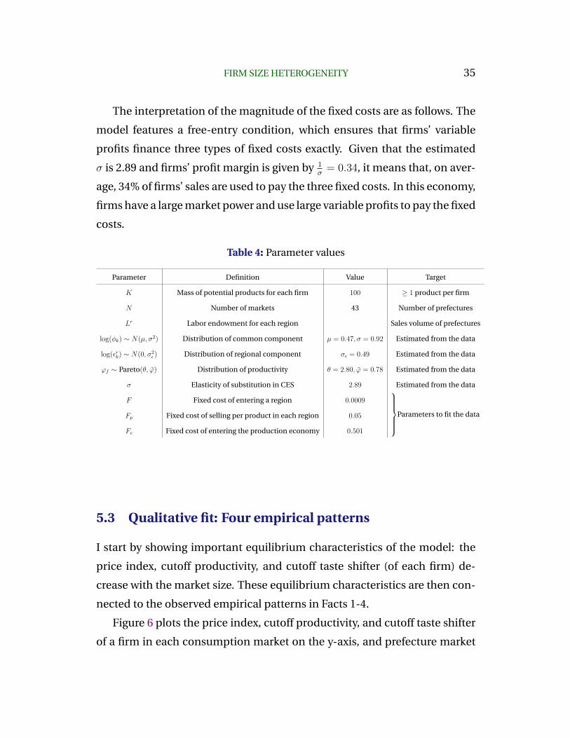
The interpretation of the magnitude of the fixed costs are as follows. The

model features a free-entry condition, which ensures that firms’ variable

profits finance three types of fixed costs exactly. Given that the estimated

σ is 2.89 and firms’ profit margin is given by 1σ

= 0.34, it means that, on aver-

age, 34% of firms’ sales are used to pay the three fixed costs. In this economy,

firms have a large market power and use large variable profits to pay the fixed

costs.

Table 4: Parameter values

Parameter Definition Value Target

K Mass of potential products for each firm 100 ≥ 1 product per firm

N Number of markets 43 Number of prefectures

Lr Labor endowment for each region Sales volume of prefectures

log(φk) ∼ N(µ, σ2) Distribution of common component µ = 0.47, σ = 0.92 Estimated from the data

log(εrk) ∼ N(0, σ2ε ) Distribution of regional component σε = 0.49 Estimated from the data

ϕf ∼ Pareto(θ, ϕ) Distribution of productivity θ = 2.80, ϕ = 0.78 Estimated from the data

σ Elasticity of substitution in CES 2.89 Estimated from the data

F Fixed cost of entering a region 0.0009

Parameters to fit the dataFp Fixed cost of selling per product in each region 0.05

Fe Fixed cost of entering the production economy 0.501

5.3 Qualitative fit: Four empirical patterns

I start by showing important equilibrium characteristics of the model: the

price index, cutoff productivity, and cutoff taste shifter (of each firm) de-

crease with the market size. These equilibrium characteristics are then con-

nected to the observed empirical patterns in Facts 1-4.

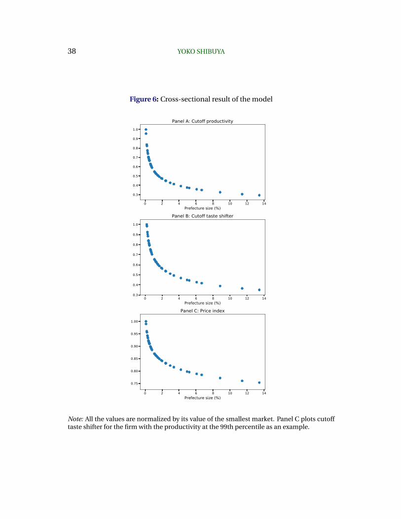
Figure 6 plots the price index, cutoff productivity, and cutoff taste shifter

of a firm in each consumption market on the y-axis, and prefecture market

36 YOKO SHIBUYA

size as a share of the aggregate market size in the economy on the x-axis.32 All

the values in the figure are normalized by the value in the smallest market.

Panel A of Figure 6 shows that the cutoff productivity decreases with the

market size. A larger market size has two offsetting effects on the cutoff pro-

ductivity. Given the price index, a larger market size means demand for each

good, allowing the lower-productivity firms to profit sufficiently to cover the

fixed cost of entering the market. A larger market size also induces more

competition across entering firms, which decreases the firms’ profits. Over-

all, the first effect dominates, and the cutoff productivity is lower in larger

markets, i.e., more firms enter larger markets. For the same reason, the cut-

off taste shifter of a given firm decreases with the market size (see Panel B

of Figure 6), which means that each firm produces more products in larger

markets.

Panel C of Figure 6 shows that the price index also decreases with the

market size. As described in Section 4.3, when more lower-productivity firms

enter larger markets, there are two offsetting effects on the price index: the

love-of-variety effect decreases the price index, while lower average produc-

tivity increases the price index. In total, the love-of-variety effect exceeds the

effect of lower average productivity; thus the price index falls with the mar-

ket size. It also means that the welfare in a market increases with the market

size; since the wage is equalized across markets, the real wage increases as

the price index decreases with the market size. Consumers in larger markets

enjoy higher welfare generated by more varieties because more firms enter

and sell more products in larger markets.33 These three cross-sectional re-

32The cutoff taste shifter in a given market differs across firms. Panel C of Figure 6 plotsthe cutoff taste shifter of the firm with productivity at 99th percentile as an example. Thedecreasing pattern of the cutoff taste shifter does not depend on the level of productivity.

33Literature in urban economics points to welfare differences across geographic locationsdue to different varieties available in each location. For example, Handbury (2019) showsthat wealthier consumers enjoy a lower price index in wealthier cities because more vari-eties that are catered to wealthier households are available in these cities.

FIRM SIZE HETEROGENEITY 37

sults are used to explain the observed patterns in Facts 1-4.

Fact 1: Larger firms penetrate smaller markets. Because the cutoff pro-

ductivity decreases with market size, only high-productivity firms enter small

markets. This follows the empirical pattern, according to which the average

firm size decreases with the market size. The model also replicates the con-

vex decreasing shape of an average firm size in the data.

Fact 2: Firms sell more products in larger markets. Panel C of Figure 6

provides direct evidence for Fact 2. It shows that the same firms have a

higher cutoff taste shifter in smaller markets, i.e., the same firms sell more

products in larger markets. The larger market size has two opposite impacts

on the cutoff taste shifter. First, a larger market size decreases the cutoff taste

shifter because there is a larger pie of consumer demand. Second, a larger

market induces more competition, which means a lower price index. All in

all, the first effect dominates, and the cutoff taste shifter decreases with the

market size, i.e., firms sell more products in larger markets.

Fact 3: Larger firms sell more products in a given market. Fact 3 is im-

plied by the cutoff taste shifter condition (6). The cutoff taste shifter condi-

tion can be rewritten as

φr∗f =

(Fp(σ − 1) σ

σ−1

Lr

) 1σ−1 1

ϕfP r. (15)

Given price index P r and market size Lr, higher productivity lowers the cut-

off taste shifter. Therefore, a higher-productivity firms sell more products

upon entering a market.

Fact 4: Firms sell different sets of products across markets. The model

fits the observed pattern of the imperfect product overlap within a firm across

markets. The model implies two mechanisms of the imperfect product over-

lap. First, the average number of products of a firm increases with the mar-

ket size. If a firm enters two markets with different market sizes, the firm

38 YOKO SHIBUYA

Figure 6: Cross-sectional result of the model

0 2 4 6 8 10 12 14Prefecture size (%)

0.3

0.4

0.5

0.6

0.7

0.8

0.9

1.0

Panel A: Cutoff productivity

0 2 4 6 8 10 12 14Prefecture size (%)

0.3

0.4

0.5

0.6

0.7

0.8

0.9

1.0

Panel B: Cutoff taste shifter

0 2 4 6 8 10 12 14Prefecture size (%)

0.75

0.80

0.85

0.90

0.95

1.00

Panel C: Price index

Note: All the values are normalized by its value of the smallest market. Panel C plots cutofftaste shifter for the firm with the productivity at the 99th percentile as an example.

FIRM SIZE HETEROGENEITY 39

sells a smaller set of products in the smaller market. Second, because of

the across-market taste heterogeneity, even if a firm enters two markets that

have identical market sizes, it produces a different set of products in each of

the markets.

5.4 Quantitative fit: firm size, product, and geographic

scope distributions

Next, I compare firm size, product scope, and geographic scope distribu-

tions in the model vs. the data (Nikkei POS). When comparing the model

and data, I plot and visually compare the firm size, product scope, and geo-

graphic scope distributions in the model and data.

As stated in Section 5.1, I estimate three fixed costs F, Fp, Fe to match

the largest 10% vs. the median firm statistics in firm size, product scope, and

geographic scope. The first row of Table 5 confirms that the model fits these

three moments in the data.

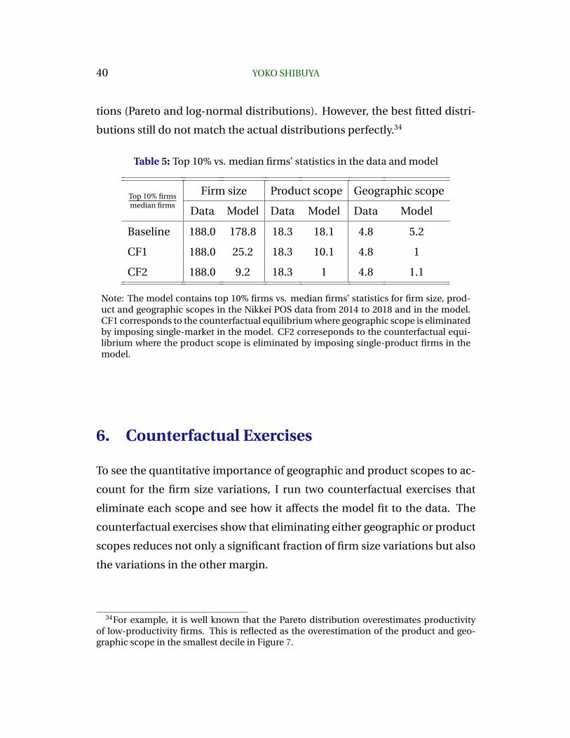
Next, I show that not only these targeted moments in the data, but the

model also replicates the observed distributions of firm size, product scope,

and geographic scope. Panel A of Figure 7 plots the log of average decile

sales normalized by top decile sales. The x-axis of the figure shows the decile

from the largest to the smallest, from right to left. The model performs well

in replicating the sales distribution. Panel B and C of Figure 7 plot the num-

ber of products and prefectures in each decile normalized by the top decile

value, respectively. The model replicates entire distributions of firms’ prod-

uct scope and geographic scope.

Overall, the model replicated the observed firm size, product scope, and

geographic scope heterogeneity well. The differences between the actual

and the predicted distributions come from the fact that I approximate the

actual productivity and taste shifter distributions by the best fitted distribu-

40 YOKO SHIBUYA

tions (Pareto and log-normal distributions). However, the best fitted distri-

butions still do not match the actual distributions perfectly.34

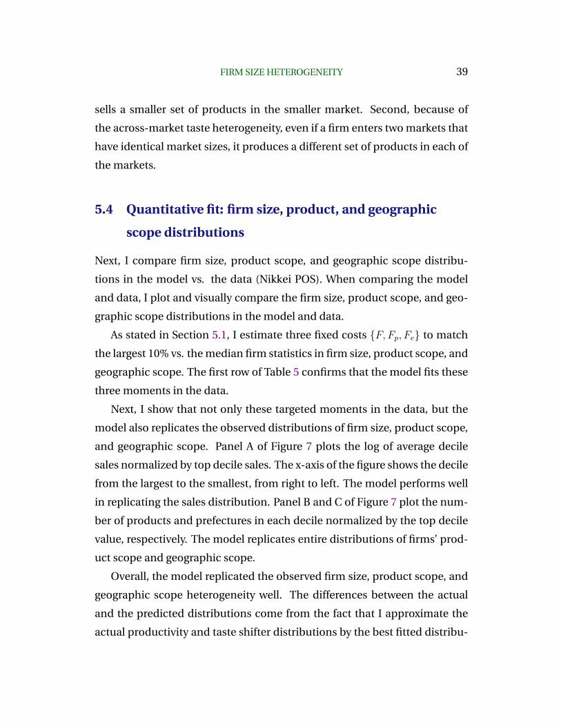
Table 5: Top 10% vs. median firms’ statistics in the data and model

Top 10% firmsmedian firms

Firm size Product scope Geographic scope

Data Model Data Model Data Model

Baseline 188.0 178.8 18.3 18.1 4.8 5.2

CF1 188.0 25.2 18.3 10.1 4.8 1

CF2 188.0 9.2 18.3 1 4.8 1.1

Note: The model contains top 10% firms vs. median firms’ statistics for firm size, prod-uct and geographic scopes in the Nikkei POS data from 2014 to 2018 and in the model.CF1 corresponds to the counterfactual equilibrium where geographic scope is eliminatedby imposing single-market in the model. CF2 correseponds to the counterfactual equi-librium where the product scope is eliminated by imposing single-product firms in themodel.

6. Counterfactual Exercises

To see the quantitative importance of geographic and product scopes to ac-

count for the firm size variations, I run two counterfactual exercises that

eliminate each scope and see how it affects the model fit to the data. The

counterfactual exercises show that eliminating either geographic or product

scopes reduces not only a significant fraction of firm size variations but also

the variations in the other margin.

34For example, it is well known that the Pareto distribution overestimates productivityof low-productivity firms. This is reflected as the overestimation of the product and geo-graphic scope in the smallest decile in Figure 7.

FIRM SIZE HETEROGENEITY 41

Figure 7: Firm size, product and geographic scope distributions in the data andmodel: Baseline

10 9 8 7 6 5 4 3 2 1Decile

0.0

0.2

0.4

0.6

0.8

1.0

Smallest Largest

DataModel

Panel A: Firm size distribution

10 9 8 7 6 5 4 3 2 1Decile

0.0

0.2

0.4

0.6

0.8

1.0

Smallest Largest

DataModel

Panel B: Product scope distribution

10 9 8 7 6 5 4 3 2 1Decile

0.2

0.4

0.6

0.8

1.0

Smallest Largest

DataModel

Panel C: Geographic scope distribution

Note: In all panels, the x-axis is the number of decile, from the smallest 10% (left) to thelargest 10% (right). Panel A shows the average firm sales in each decile in the data and themodel. The average decile sales are normalized by the top decile sales. Panel B shows theaverage number of products of the firms in each decile in the data and the model. Theaverage number of products in each decile is normalized by the top decile value. Panel Cshows the average number of markets that firms in each decile sell at least one product in.Again, the values are normalized by the top decile value.

42 YOKO SHIBUYA

CF1: Eliminating geographic scope

To eliminate geographic margin from the model, I solve a single-market ver-

sion of the model. Specifically, I assume that there is a single market in the

economy in which the labor endowment is equal to the average labor en-

dowment in the original economy, i.e., L = 1N

ΣrLr.

Moving from the original to the single-market model shuts off geographic

scope variations across firms because all the surviving firms enter one mar-

ket. Therefore, compared with the original equilibrium, where higher-productivity

firms enter more markets and acquire larger revenues, the firm size varia-

tions are expected to be smaller. In addition, unlike the original equilibrium

where firms sell different sets of products across markets due to consumer

taste heterogeneity, the product scope variations are expected to be smaller

in the single-market model.

The second column of Table 5 reports the result from eliminating geo-

graphic scope. First, because I eliminate geographic scope, the top 10%

firms vs. median firms’ value of the geographic scope is reduced from 4.8

to 1 in terms of the top 10% vs. median firms’ values. Second, product scope

heterogeneity is also reduced by 45% (from 18.3 to 10.1). This is explained by

a lack of complementarity between geographic and product scope through

consumer taste heterogeneity across markets. In total, moving from the

multiple-market to the single-market models reduces firm size heterogene-

ity by 86% (from 188 to 25.2).35

35Another way to eliminate geographic scope is to assume symmetric market size acrossmarkets. As an alternative counterfactual exercise, I impose a symmetric market size as-sumption with labor endowment in each market equal to the average labor endowment inthe original economy, Lr = 1

N ΣrLr. It reduces product scope heterogeneity by 28% (18.3

to 13.1) and firm size heterogeneity by 53% (188 to 88.4). The difference between the origi-nal and alternative counterfactual exercise is the total market size in the economy. Becausethe alternative exercise has a larger market size of the economy, it involves a larger mass offirms, and thus, competition is harsher.

FIRM SIZE HETEROGENEITY 43

CF2: Eliminating product scope

To eliminate product scope from the model, I solve a single-product firm

version of the model. Specifically, each firm is endowed with one product for

which the taste shifter equals one in any consumption market. The demand

for the product of firm f in market r equals

Crf =

( pfP r

)−σ LrP r.

The model is now similar to Melitz (2003) but with asymmetric market size.

Moving from the original to the single-product firm model shuts off prod-

uct scope variations across firms because all the surviving firms produce

only one product. Therefore, compared with the original equilibrium where

higher-productivity firms produce more products and acquire larger rev-

enues, the firm size variations are expected to be smaller. In addition, un-

like the original equilibrium, where higher-productivity firms produce more

products in a given market, when all the firms produce only one product,

lower-productivity firms have a higher chance to enter the market. There-

fore, geographic scope variations are expected to be smaller as well.

The third column of Table 5 reports the result of eliminating product

scope. When product scope heterogeneity is completely eliminated (18.8 to

1), geographic scope heterogeneity is also reduced by 77% (from 4.8 to 1.1)

in terms of the top 10% versus median firms’ values. This is due to the lack of

complementarity between product and geographic scopes described above.

In total, moving from the multi-product firm model to the single-product

firm model reduces firm size heterogeneity by 95% (from 188.8 to 9.2).

The two counterfactuals show that complementarity between product

and geographic scope is quantitatively important. Existing models of firm

heterogeneity with only either one of the extensive margins miss firm size

heterogeneity due to a lack of variation in missed margin but also the vari-

44 YOKO SHIBUYA

ation in the other margin coming from complementarity between the two

margins. It should be noted that these counterfactual exercises are con-

ducted with all the parameters value fixed at the baseline values presented

in Table 4. In Appendix A.3.2, I explain how parameter values change if the

model is re-estimated to match the top 10% vs. the median firm statistics in

firm size, product scope, and geographic scope in two counterfactual exer-

cises.

7. Efficiency of the market equilibrium and

welfare implication of size-dependent policies

I solve the social planner’s problem and show that the market equilibrium is

efficient. Given the result, I discuss the welfare implication of sub-optimal

size-dependent policies, taking actual policy in Japan as an example. I com-

pare the welfare cost between the baseline and single-product firm model

and find that the missing product scope margin largely underestimates the

welfare cost of such policies.

7.1 Social planner’s problem

It is well known that the market equilibrium in my baseline model, Melitz

(2003), is efficient.36To understand whether this efficiency is carried over

when multi-product firms and multiple regions with heterogeneous mar-

ket sizes are added, I solve the social planner’s problem, whose objective is

to maximize the real consumption index of the representative consumers in

the economy.

36For example, Melitz and Redding (2015) show that with CES preferences and monopo-listic competition, the open economy equilibrium in the heterogeneous firm model is effi-cient. Dhingra and Morrow (2019) analyze the efficiency of heterogeneous firm models in amore generalized setting.

FIRM SIZE HETEROGENEITY 45

The real consumption index for the representative consumer in the econ-

omy is defined as

Q = Σrβr

[M

∫ ∞ϕrs

K

∫ ∞φr∗s,f

(φrk,fC

rk,f

)σ−1σ dF (φrkf )dG(ϕf )

] σσ−1

, (16)

where βr is the welfare weight on the real consumption index of each mar-

ket r. The welfare weight is set as proportional to the labor endowment,

i.e., βr = Lr∑r L

r . For each consumption market r, the social planner chooses

the productivity cutoff ϕrs, the taste shifter cutoff φrf,s for all producing firms

ϕf ≥ ϕrs, and the output level Crk,f for all produced goods φrk,f ≥ φrf,s for all

producing firms ϕf ≥ ϕrs. Lastly, the planner chooses the mass of firms M

subject to the aggregate labor constraint:

ΣrLr = ΣrM

∫ ∞ϕrs

K

∫ ∞φr∗s,f

Crk,f

ϕf+ FpdF (φrkf )dG(ϕf ) +

∫ ∞ϕrs

FdG(ϕf ) + Fe

,

(17)

where the social planner faces the same productivity distributionG(ϕf ), taste

shifter distribution F (φrk,f ), and fixed costs. The following proposition sum-

marizes the social planner’s choice with general distributions of productivity

and taste shifter.

Proposition 1 The social planner’s choice of the output level, taste shifter cut-

off, productivity cutoff, and mass of firms entering the economy coincides with

the market allocation, i.e., the market equilibrium is efficient.

The proof of this proposition is presented in Appendix A.4.

The intuition behind the efficiency of the market equilibrium is the fol-

lowing. First, the CES utility function and monopolistic competition leads

to constant markups across firms, σσ−1

. Therefore, there is no markup distor-

tion across products or firms; hence the output level in the market equilib-

rium is optimal. Next, as for the taste shifter cutoff and productivity cutoff,

46 YOKO SHIBUYA

there are two sources of potential inefficiency. When introducing another

product or firm, firms do not internalize the positive effect on consumer

surplus (the love-of-variety effect) and the negative effect on the sales of

other products and firms (the business-stealing effect). The CES utility func-

tion uniquely ensures that these two externalities exactly offset each other.

Lastly, as for the mass of firms in the economy, a potential inefficiency comes

from the fact that, with heterogeneous productivity, some firms make profits

and some others make a loss. A free-entry condition ensures that the profits

and losses exactly finance the fixed costs of entering, which means that the

mass of firms entering the economy is at an efficient level. Therefore, the

market implements the efficient allocation.

7.2 Welfare cost of sub-optimal SME subsidies

The efficiency of the market equilibrium implies that any policy distorting

the market allocation is sub-optimal. In this section, I estimate the social

cost of the subsidies for Small and Medium Enterprises (SMEs) to expand

their geographic scope, a policy tool frequently used in Japan. I consider

two cases: the baseline and the single-product firms. Comparison between

the welfare costs of the subsidies under the baseline model and the single-

product firm model allows us to measure the importance of having both

product and geographic scopes for quantifying effects of size-dependent poli-

cies.

7.2.1 SME subsidies in Japan

Although my model suggests that the market equilibrium with a vast dif-

ference in firm performance is efficient, the Japanese government has con-

FIRM SIZE HETEROGENEITY 47

ducted various policies to promote SME growth.37 One of the main policy

tools to promote SME growth is subsidy for SMEs to expand their markets.

There are many types of subsidies for SMEs to expand their markets.38

Coverage and financial sources of the subsidies vary across different types of

subsidies, but most of them share the eligibility requirement and the types

of costs that are subsidized. The condition for the companies to be eligible

for subsidies is to have equity or employment less than a cutoff value.39 The

types of the costs covered by subsidies include the fees of joining supplier-

buyer matching events, traveling expenses to meet buyers, and the costs as-

sociated with making new contracts with buyers.

Among these SME subsidies, I take the subsidy provided by the Tokyo

Metropolitan Small and Medium Enterprise Support Center (a government

owned financial agency) in 2020-2021 financial year as an example to ana-

lyze the welfare cost of the subsidy. This particular SME subsidy aims to pro-

mote growth of the SMEs located in Tokyo prefecture; there are also similar

SME subsidies available at government owned financial agencies. The firms

eligible for the subsidy are manufacturing firms with less than 300 employ-

ees. Whether a particular firm is eligible for the subsidy is determined based

on the number of employees listed in the previous year’s tax return docu-

ments of the enterprise tax. The subsidy covers the costs of participating in

supplier-buyer matching events (including the participation fee, traveling

costs, etc). The coverage of the subsidy is up to two-thirds of the total costs.

The total costs are first paid by the companies, and the agency reviews the

37The rationale for the Japanese government to support SMEs growth that is not capturedin my model includes the political power of SMEs. Since SMEs represent 70% of all employ-ment in Japan, the voting power of SMEs is larger than their economic presence.

38For example, a list of subsidies available as of June 4th, 2021 can be found here https://hojyokin-portal.jp/subsidies/list. Note that the website is available only in Japanese.

39For the manufacturing firms, the usual cutoff values are 300 million Japanese yen (ap-proximately 3 million USD) for equity and 300 people for employment. Firms in the serviceand other industries have lower cutoff values.

48 YOKO SHIBUYA

receipts and determines whether these costs are eligible for a subsidy. Af-

ter getting it approved by the agency, two-thirds of the costs are reimbursed

back to the companies.40

7.2.2 Modeling the SME subsidy

The eligibility, types of the costs covered by the subsidy, and the coverage of

the subsidy are modeled in the following ways. In the model, firms’ employ-

ments have a one-to-one relationship with their productivity, i.e., higher-

productivity firms use more labor. Thus, imposing an eligibility threshold

for the subsidy by employment (less than 300 employess) is identical to im-

posing an eligibility threshold on productivity in the model.41 Define ϕ∗s as

the threshold productivity allowing the firms with the productivity below the

threshold to be considered eligible for a subsidy. Because the firms who have

less than 300 employees comprise 98.5% of all firms in the manufacturing in-

dustry in Japan, I set ϕ∗s such that surviving firms with productivity less than

ϕ∗s consist of 98.5% of all surviving firms:

G(ϕ∗s)−G(ϕ∗)

1−G(ϕ∗)= 0.985, (18)

where ϕ∗ is the smallest cutoff productivity in the market equilibrium (be-

fore the subsidy is imposed).42

40See more detail about the subsidy in https://www.tokyo-kosha.or.jp/support/josei/jigyo/hankaku.html. Note that the document is available only in Japanese.

41One caveat is that, in reality, firms may modify their number of employees to becomeeligible for a subsidy. However, a firm’s eligibility is determined based on the previous year’stax return documents, and the announcement of the subsidy was made after the deadlinefor the tax document. Therefore, I conclude that firms did not decrease their number ofemployees to become eligible for the subsidy.

42In the model, there is no location of firms, so it is not possible to distinguish firms inthe Tokyo prefecture from firms in the other prefectures. Since similar types of SME subsidyare available in most prefectures in Japan, I assume that all prefectures in Japan provide thesame type of subsidies. Therefore, it is deduced that a subsidy is available for all firms thatare below the productivity threshold of the subsidy.

FIRM SIZE HETEROGENEITY 49

Lastly, the costs covered by the actual subsidy correspond to the fixed

cost of entering a market, F , in the model. Define s as a fraction of subsidy

for the fixed cost of entering a market. Then, the government provides sub-

sidy for the firms whose productivity is less than the threshold productivity

ϕ∗s, i.e., the fixed cost of entering a market = (1 − s)F for the firms with pro-

ductivity ϕf ≤ ϕ∗s. Lastly, to be consistent with the actual coverage of the

subsidy, I set s = 23

in the model.

I assume a balanced budget in each consumption market by imposing

lump-sum income tax on consumers. The representative consumer’s budget

constraint becomes∫f∈Ωr

∫kf∈Ωrf

prkfCrkf

dkf df ≤ Lr − T r. (19)

The lump-sum tax T r is given by

T r = M

∫ ϕ∗s

ϕr∗sF dG(ϕf ), (20)

where the subsidy is granted for the firms entering market r (ϕf ≥ ϕr∗) but

with the productivity less than the threshold (ϕf ≤ ϕ∗s). In the single-product

firm model, the representative consumer’s budget constraint becomes∫f∈Ωr

prkfCrkf

df ≤ Lr − T r, (21)

where product kf denotes a single product produced by firm f . The lump-

sum income tax amount T r follows the same expression as in the baseline

model shown in (20).

50 YOKO SHIBUYA

7.2.3 Results: baseline and single-product market model

Moving from the market equilibrium to the equilibrium under the subsidy

affects the real consumption index of each market in the following way. The

firms whose productivity is less than the threshold productivity receive a

subsidy to cover the fixed cost of entering a market; thus they are more likely

to enter the market. The subsidy is financed by a lump-sum income tax,

which is borne by all the entering firms as a reduction in total consumer de-

mand, including the high-productivity firms that do not receive the subsidy.

Furthermore, because of the entry of more firms due to the subsidy, the com-

petition within a market becomes harsher. In total, the subsidy helps the

low-productivity firms enter more markets but hurts the high-productivity

firms’ profits.

In the baseline model, the subsidy results in the loss of the real con-

sumption index in the economy by 1.25%. In the model with single-product

firms, the welfare costs of the subsidy are reduced to 0.58% of the real con-

sumption index. There are two reasons why the single-product firm model

underestimates the cost of the subsidy. First, the subsidy helps the lower-

productivity firms to enter the market, but these firms only sell one product.

Thus, the entry of lower-productivity firms induces a minor competition in-

crease. Second, the high-productivity firms that suffer from the reduction

in total consumer demand sell only one product with and without subsidy.

Therefore, higher-productivity firms’ product scope margin is not distorted,

and the only effect is reflected on their intensive margins. Taken together,

the single-product firm model underestimates the welfare cost of the SME

subsidies.

Furthermore, the subsidy affects different markets differently. The sub-

sidy hits larger markets harder because larger markets have lower cutoff firm

productivity, and more, lower productivity firms receive a subsidy to en-

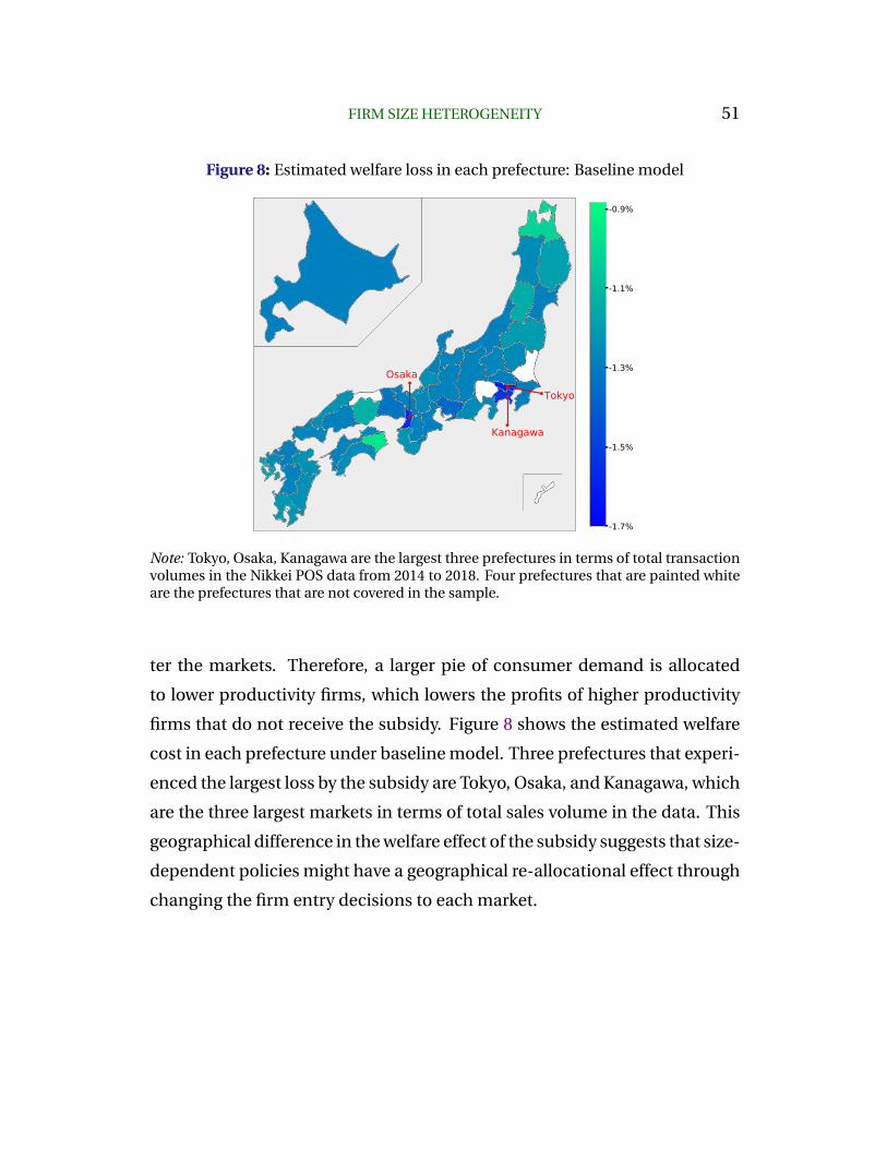
FIRM SIZE HETEROGENEITY 51

Figure 8: Estimated welfare loss in each prefecture: Baseline model

OsakaTokyo

Kanagawa

-1.7%

-1.5%

-1.3%

-1.1%

-0.9%

Note: Tokyo, Osaka, Kanagawa are the largest three prefectures in terms of total transactionvolumes in the Nikkei POS data from 2014 to 2018. Four prefectures that are painted whiteare the prefectures that are not covered in the sample.

ter the markets. Therefore, a larger pie of consumer demand is allocated

to lower productivity firms, which lowers the profits of higher productivity

firms that do not receive the subsidy. Figure 8 shows the estimated welfare

cost in each prefecture under baseline model. Three prefectures that experi-

enced the largest loss by the subsidy are Tokyo, Osaka, and Kanagawa, which

are the three largest markets in terms of total sales volume in the data. This

geographical difference in the welfare effect of the subsidy suggests that size-

dependent policies might have a geographical re-allocational effect through

changing the firm entry decisions to each market.

52 YOKO SHIBUYA

8. Conclusion

The recent literature in firm heterogeneity has documented the importance

of two extensive margins to account for firm size heterogeneity: product and

geographic scopes. Although much attention has been paid to the role of

each extensive margin separately, I argue in this paper that the two extensive

margins interact in a major way and thus, for the need to have both extensive

margins in one model. I develop a heterogeneous-firm model with multi-

product firms and multiple markets that comprise consumers with hetero-

geneous tastes. In the model, firms’ decisions on product and geographic

scopes interact in two ways. First, as firms expect to sell more products and

larger profits, they are more likely to enter a market. Second, as firms en-

ter more markets, they sell greater varieties of products because each mar-

ket exhibits different consumer tastes. The calibrated model reveals that

each complementarity is quantitatively important. Eliminating either ge-

ographic or product scope from the model reduces firm size variations by 86

to 94%, failing to incorporate the complementarity between two margins. I

further use the model to quantify the welfare implication of the actual size-

dependent subsidy in Japan. Notably, the model with only a single extensive

margin underestimates the welfare implication of such subsidies by more

than half.

There are a couple of additional directions for research suggested by the

paper. First, my analysis focuses on explaining cross-sectional firm size vari-

ations, and it is left unknown how the firms’ performance and product and

geographic scopes evolve. Exploring these aspects requires access to panel

data that would allow analyzing observations made over some course of

time. Second, my framework does not incorporate distance. Including dis-

tance in the model lets us explore what role shipping costs and taste hetero-

geneity, which are correlated with the distance between the markets, play in

FIRM SIZE HETEROGENEITY 53

generating firm size heterogeneity.

References

Arkolakis, Costas, “Market penetration costs and the new consumers margin in in-

ternational trade,” Journal of political economy, 2010, 118 (6), 1151–1199.

, Sharat Ganapati, and Marc-Andreas Muendler, “The extensive margin of export-

ing products: A firm-level analysis,” Technical Report, National Bureau of Eco-

nomic Research 2010.

Atkin, David, “Trade, tastes, and nutrition in India,” American economic review,

2013, 103 (5), 1629–63.

Bagwell, Kyle and Asher Wolinsky, “Game theory and industrial organization,”

Handbook of Game Theory with Economic Applications, 2002, 3, 1851–1895.

and Garey Ramey, “Coordination economies, advertising, and search behavior

in retail markets,” The American Economic Review, 1994, pp. 498–517.

Bartelsman, Eric, John Haltiwanger, and Stefano Scarpetta, “Cross-country differ-

ences in productivity: The role of allocation and selection,” American economic

review, 2013, 103 (1), 305–34.

Bernard, Andrew B, Emmanuel Dhyne, Glenn Magerman, Kalina Manova, and An-

dreas Moxnes, “The origins of firm heterogeneity: A production network ap-

proach,” Technical Report, National Bureau of Economic Research 2019.

, Stephen J Redding, and Peter K Schott, “Multiple-product firms and product

switching,” American Economic Review, 2010, 100 (1), 70–97.

, , and , “Multiproduct firms and trade liberalization,” The Quarterly journal

of economics, 2011, 126 (3), 1271–1318.

54 YOKO SHIBUYA

Bronnenberg, Bart J, Jean-Pierre H Dube, and Matthew Gentzkow, “The evolution

of brand preferences: Evidence from consumer migration,” American Economic

Review, 2012, 102 (6), 2472–2508.

, Sanjay K Dhar, and Jean-Pierre H Dube, “Brand history, geography, and the per-

sistence of brand shares,” Journal of political Economy, 2009, 117 (1), 87–115.

Choi, Jeonghye and David R Bell, “Preference minorities and the Internet,” Journal

of Marketing Research, 2011, 48 (4), 670–682.

Dhingra, Swati and John Morrow, “Monopolistic competition and optimum prod-

uct diversity under firm heterogeneity,” Journal of Political Economy, 2019, 127

(1), 196–232.

Eaton, Jonathan, Samuel Kortum, and Francis Kramarz, “An anatomy of interna-

tional trade: Evidence from French firms,” Econometrica, 2011, 79 (5), 1453–1498.

Eckel, Carsten and J Peter Neary, “Multi-product firms and flexible manufacturing

in the global economy,” The Review of Economic Studies, 2010, 77 (1), 188–217.

Fernandes, Ana M, Peter J Klenow, Sergii Meleshchuk, Martha Denisse Pierola, and

Andres Rodriguez-Clare, “‘The Intensive Margin in Trade: How Big and How Im-

portant?,” Unpublished manuscript, 2019.

Handbury, Jessie, “Are poor cities cheap for everyone? non-homotheticity and the

cost of living across us cities,” Technical Report, National Bureau of Economic

Research 2019.

Hopenhayn, Hugo A, “Entry, exit, and firm dynamics in long run equilibrium,”

Econometrica: Journal of the Econometric Society, 1992, pp. 1127–1150.

Hottman, Colin J, Stephen J Redding, and David E Weinstein, “Quantifying the

sources of firm heterogeneity,” The Quarterly Journal of Economics, 2016, 131 (3),

1291–1364.

FIRM SIZE HETEROGENEITY 55

Hulcr, Jiri, Prarthana S Dharampal, Ronda L Hamm, Gwen Pearson, and Cara Gib-

son, “Influence Is Power: Strategic Communication for Entomologists,” American

Entomologist, 2019, 65 (2), 92–96.

Jovanovic, Boyan, “Selection and the Evolution of Industry,” Econometrica: Journal

of the Econometric Society, 1982, pp. 649–670.

Luttmer, Erzo GJ, “Selection, growth, and the size distribution of firms,” The Quar-

terly Journal of Economics, 2007, 122 (3), 1103–1144.

Mayer, Thierry, Marc J Melitz, and Gianmarco IP Ottaviano, “Market size, compe-

tition, and the product mix of exporters,” American Economic Review, 2014, 104

(2), 495–536.

Melitz, Marc J, “The impact of trade on intra-industry reallocations and aggregate

industry productivity,” econometrica, 2003, 71 (6), 1695–1725.

and Stephen J Redding, “New trade models, new welfare implications,” American

Economic Review, 2015, 105 (3), 1105–46.

Ossa, Ralph, “Trade wars and trade talks with data,” American Economic Review,

2014, 104 (12), 4104–46.

Quan, Thomas W and Kevin R Williams, “Product variety, across-market demand

heterogeneity, and the value of online retail,” The RAND Journal of Economics,

2018, 49 (4), 877–913.

Startz, Meredith, “The value of face-to-face: Search and contracting problems in

Nigerian trade,” Available at SSRN 3096685, 2016.

Waldfogel, Joel, “Preference Externalities: An Empirical Study of Who Benefits

Whom in Differentiated-Product Markets,” RAND Journal of Economics, 2003, 34

(3), 557–68.

, “The median voter and the median consumer: Local private goods and popula-

tion composition,” Journal of urban Economics, 2008, 63 (2), 567–582.

56 YOKO SHIBUYA

, Thomas J Holmes, and Roger G Noll, “Who benefits whom in local television

markets?[with comments],” Brookings-Wharton Papers on Urban Affairs, 2004,

pp. 257–305.

A. Appendix

A.1 Retail chains and firm sizes

This section answers whether larger firms are connected to a few larger retail

chains and sell their products in many stores within the few retail chains.

My data shows that this is not the case; larger firms sell in more retail chains,

and these retail chains are not systematically larger than the retail chains

that smaller firms are connected.

The first column of Table 6 shows the average number of prefectures that

firms sell their products in increases with firm size. If larger firms have a

wider geographic scope because they sell to a few retail chains with many

stores in many prefectures, then I would expect the average number of retail

chains to not increase with firm size. The second column of Table 6 shows

that the average number of retail chains monotonically increases with firm

size. It means that larger firms sell not only in many prefectures but also in

many retail chains.

I also check whether the retail chains that larger firms connect have more

stores than those that smaller firms connect. The last column of Table 6

shows that it is not the case; the average number of stores per retail chain

does not increase monotonically with firm size. The smallest 10% firms sell

to retail chains that have, on average, the largest number of stores. The find-

ings in Table 6 suggest that the reason why larger firms sell their products in

more prefectures is not that they sell to large retail chains, but they sell to

many retail chains and stores.

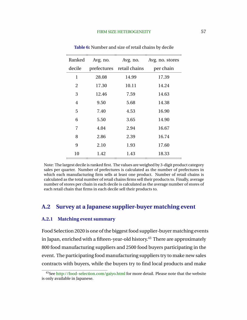
FIRM SIZE HETEROGENEITY 57

Table 6: Number and size of retail chains by decile

Ranked

decile

Avg. no.

prefectures

Avg. no.

retail chains

Avg. no. stores

per chain

1 28.08 14.99 17.39

2 17.30 10.11 14.24

3 12.46 7.59 14.63

4 9.50 5.68 14.38

5 7.40 4.53 16.90

6 5.50 3.65 14.90

7 4.04 2.94 16.67

8 2.86 2.39 16.74

9 2.10 1.93 17.60

10 1.42 1.43 18.33

Note: The largest decile is ranked first. The values are weighed by 3-digit product categorysales per quarter. Number of prefectures is calculated as the number of prefectures inwhich each manufacturing firm sells at least one product. Number of retail chains iscalculated as the total number of retail chains firms sell their products to. Finally, averagenumber of stores per chain in each decile is calculated as the average number of stores ofeach retail chain that firms in each decile sell their products to.

A.2 Survey at a Japanese supplier-buyer matching event

A.2.1 Matching event summary

Food Selection 2020 is one of the biggest food supplier-buyer matching events

in Japan, enriched with a fifteen-year-old history.43 There are approximately

800 food manufacturing suppliers and 2500 food buyers participating in the

event. The participating food manufacturing suppliers try to make new sales

contracts with buyers, while the buyers try to find local products and make

43See http://food-selection.com/gaiyo.html for more detail. Please note that the websiteis only available in Japanese.

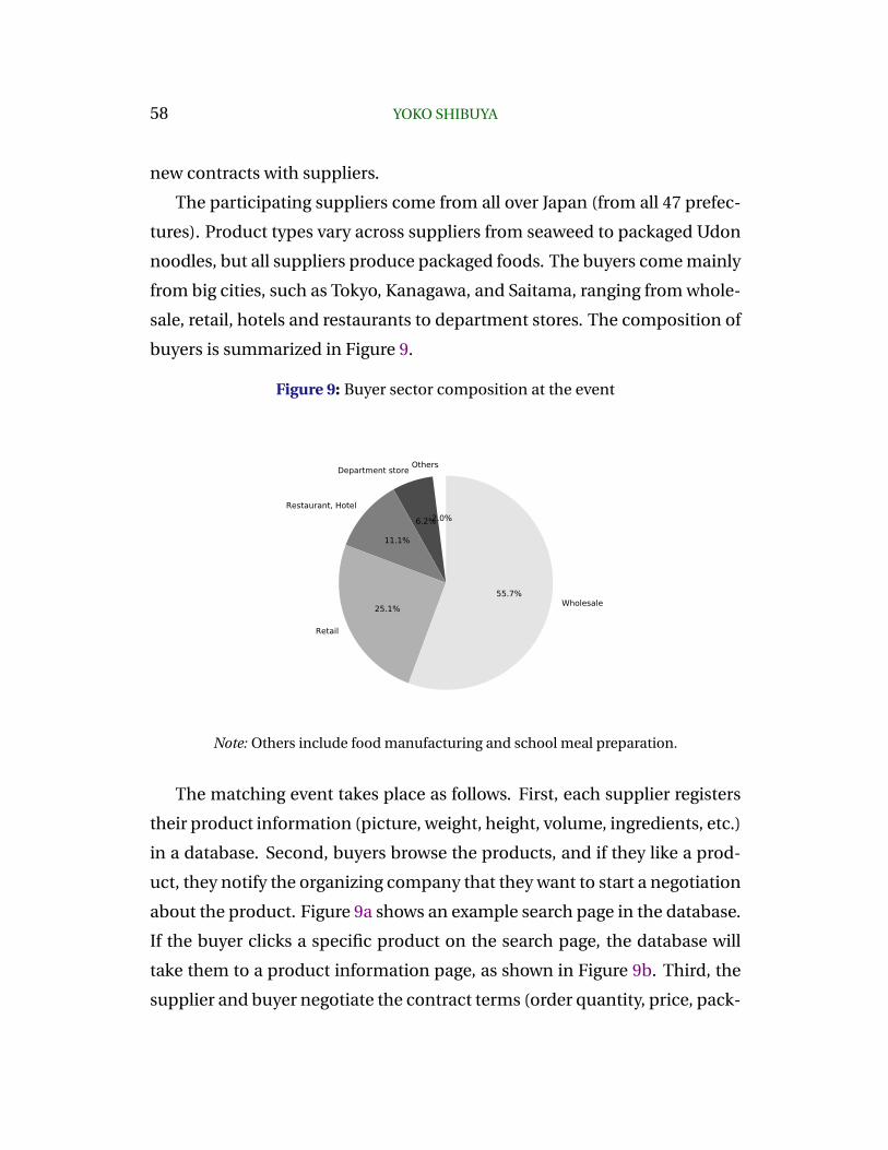
58 YOKO SHIBUYA

new contracts with suppliers.

The participating suppliers come from all over Japan (from all 47 prefec-

tures). Product types vary across suppliers from seaweed to packaged Udon

noodles, but all suppliers produce packaged foods. The buyers come mainly

from big cities, such as Tokyo, Kanagawa, and Saitama, ranging from whole-

sale, retail, hotels and restaurants to department stores. The composition of

buyers is summarized in Figure 9.

Figure 9: Buyer sector composition at the event

Others

2.0%

Department store

6.2%Restaurant, Hotel

11.1%

Retail

25.1% Wholesale55.7%

Note: Others include food manufacturing and school meal preparation.

The matching event takes place as follows. First, each supplier registers

their product information (picture, weight, height, volume, ingredients, etc.)

in a database. Second, buyers browse the products, and if they like a prod-

uct, they notify the organizing company that they want to start a negotiation

about the product. Figure 9a shows an example search page in the database.

If the buyer clicks a specific product on the search page, the database will

take them to a product information page, as shown in Figure 9b. Third, the

supplier and buyer negotiate the contract terms (order quantity, price, pack-

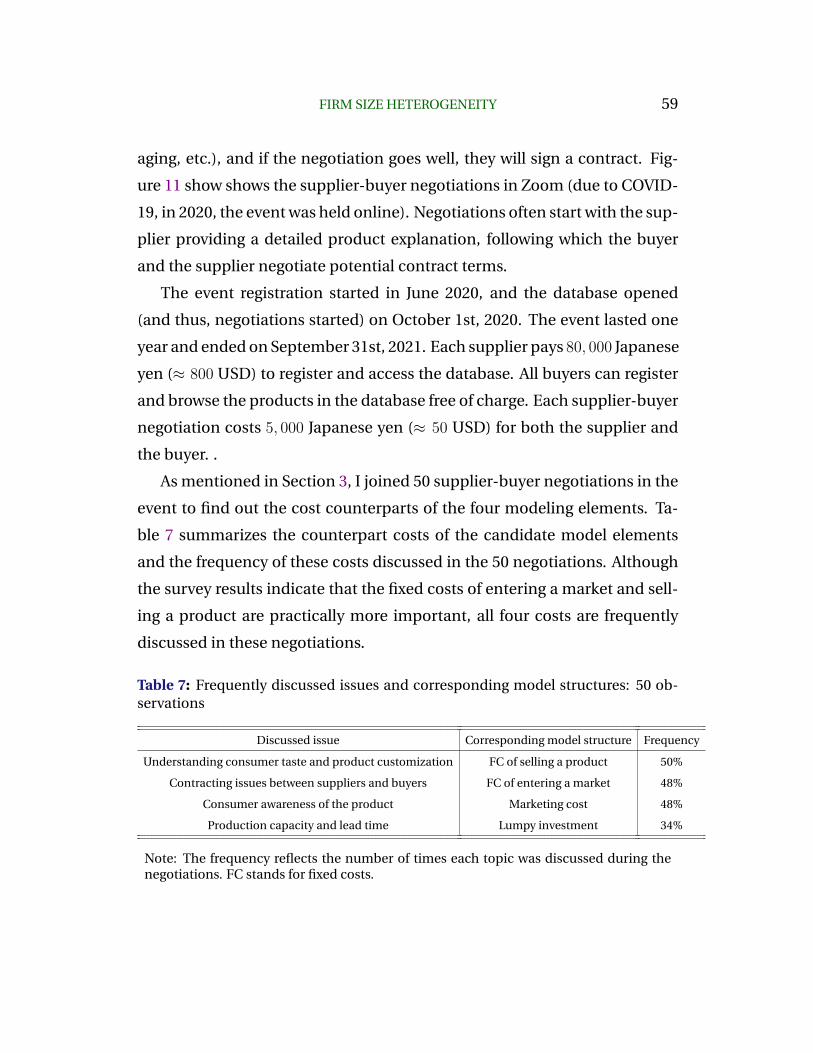
FIRM SIZE HETEROGENEITY 59

aging, etc.), and if the negotiation goes well, they will sign a contract. Fig-

ure 11 show shows the supplier-buyer negotiations in Zoom (due to COVID-

19, in 2020, the event was held online). Negotiations often start with the sup-

plier providing a detailed product explanation, following which the buyer

and the supplier negotiate potential contract terms.

The event registration started in June 2020, and the database opened

(and thus, negotiations started) on October 1st, 2020. The event lasted one

year and ended on September 31st, 2021. Each supplier pays 80, 000 Japanese

yen (≈ 800 USD) to register and access the database. All buyers can register

and browse the products in the database free of charge. Each supplier-buyer

negotiation costs 5, 000 Japanese yen (≈ 50 USD) for both the supplier and

the buyer. .

As mentioned in Section 3, I joined 50 supplier-buyer negotiations in the

event to find out the cost counterparts of the four modeling elements. Ta-

ble 7 summarizes the counterpart costs of the candidate model elements

and the frequency of these costs discussed in the 50 negotiations. Although

the survey results indicate that the fixed costs of entering a market and sell-

ing a product are practically more important, all four costs are frequently

discussed in these negotiations.

Table 7: Frequently discussed issues and corresponding model structures: 50 ob-servations

Discussed issue Corresponding model structure Frequency

Understanding consumer taste and product customization FC of selling a product 50%

Contracting issues between suppliers and buyers FC of entering a market 48%

Consumer awareness of the product Marketing cost 48%

Production capacity and lead time Lumpy investment 34%

Note: The frequency reflects the number of times each topic was discussed during thenegotiations. FC stands for fixed costs.

60 YOKO SHIBUYA

Figure 10: An overview of the database

(a) A search page example. (b) A product information example.

Figure 11: An overview of online negotiations

(a) A supplier explaining the productionprocess.

(b) A supplier explaining the product infor-mation.

A.2.2 Survey design and response rates

The survey targeted all the suppliers who participated in the event (802 firms

from 47 prefectures in Japan) and was designed to be filled in online through

a Google Form. The survey questions were incorporated into the event sur-

vey circulated by the organizing company in April 2021 to obtain the partic-

ipants’ feedback about the event.

FIRM SIZE HETEROGENEITY 61

The objective of the survey for this paper was to determine the relative

importance among the four modeling elements generating product or geo-

graphic scope variations across firms and choose my model structures that

are of the highest practical importance. As it was elaborated in Section 3,

the four candidate model elements suggested by the literature are the fixed

costs of entering a market and selling a product, the marketing cost, and the

cost of investment into production capital.

Based on the observations of 50 supplier-buyer negotiations (see Table 7),

I find that the fixed cost of entering a market corresponds to the cost of

making a contract with buyers, and the fixed cost of selling a product cor-

responds to the cost of researching consumer taste and product customiza-

tion. The marketing cost and the cost of investment into production capital

have the straightforward corresponded costs in reality. Therefore, to deter-

mine the relative importance between the four model elements, I ask the

suppliers the relative importance of the four types of costs each correspond-

ing to one of the model elements. In the online survey, I asked the suppli-

ers the following question. On the scale of 1 to 4 (1: not important to 4:

very important), how important are the following elements when expanding

into new geographic markets? (1) overcoming contracting issues with buy-

ers, (2) understanding consumer taste and customizing products to cater to

the taste, (3) having sufficient production capacity for the new market, and

(4) advertising products to increase consumer awareness.

Out of the 802 targeted suppliers, I got responses from 246 suppliers (i.e.,

31% response rate). The respondent suppliers come from a wide range of

geographic areas from 34 out of 47 prefectures in Japan. Since the survey

requires knowledge about the relative importance of business barriers, it is

important to make sure that the respondents have enough knowledge about

the companies’ businesses. Out of 246 respondents, 39% are CEO/presidents,

16% are executive managing directors, 23% are department chief/general

62 YOKO SHIBUYA

managers, and the rest 22% of the respondents are either sales staff or op-

erators.

A.3 More explanation on structural estimation

Section s:simulation-algorithm explains simulation algorithm used in the

SMM, and Section 6 explains the re-estimation of the parameter values in

the counterfactual exercises.

A.3.1 Simulation algorithm

The given simulation of the model requires a set of parameters Θ2 = σ, (θ, ϕ),the data for product- and firm-level sales, (firm-level) prices, and number of

products firms sell in each market. It involves the following steps:

Preparation: Draw productivity of 100,000 artificial Japanese firms from

the following distribution: ϕf ∼ Pareto(θ, ϕ), given assumed values of θ and

ϕ.

Step 1. Among these artificial Japanese firms, randomly sample 10,000

firms in each simulation. Among the 10,000 artificial firms, use the surviv-

ing firms, i.e., the firms with the productivity higher than the lowest cutoff

productivity, for the remaining simulation.

Step 2. Calculate the prices of the surviving firms by expression 3. Note

that, in my model, the firms’ pricing depends only on productivity (ϕf ) and

the elasticity of substitution (σ).

Step 3. For the surviving firms, drawK common components of the taste

shifter for each product from the distribution: log(φk) ∼ N(µ, σ2). Simi-

larly, for each product and each market, draw the regional shock of the taste

shifter from the distribution: log(εrk) ∼ N(0, σ2ε ).

Step 4. Compute the number of products firms produce in each market

by the cutoff taste-shifter condition (6).

FIRM SIZE HETEROGENEITY 63

Step 5. Compute the product-level sales for each firm in each market by

the following expression:

prfCrk,f = (φf )

σ−1( pfP r

)1−σLr. (22)

Compute the firm-level sales in each market by the following expression:∫kf∈Ωrf

pfCrk,f dkf =

∫kf∈Ωrf

(φf )σ−1( pfP r

)1−σLr dkf . (23)

Step 6. Estimate σ using expression (10) and ϕf for each surviving firm

from expression (11).

Step 7. Compute the best-fitted scale and shape parameters for the esti-

mated productivity distribution: ϕf ∼ Pareto(θ, ϕ).

These seven steps produce the biased estimates of σ, (θ, ϕ). The weigh-

ing matrix is calculated as a variance-covariance matrix of the error function

using the following bootstrap procedure: (i) re-sample, with replacement,

10,000 firms from our initial data set of the 100,000 firms 1000 times. (ii) For

each re-sampling b, calculate moments m(Θ2). (iii) Calculate

W2 =1

1000

1000∑b=1

(mb2 −mb(Θ2))(mb

2 −mb(Θ2))′. (24)

A.3.2 Re-estimation of the parameter values

In the counterfactual exercises conducted in Section 6, I check how the firm

size, the product and geographic scope distributions change when eliminat-

ing one of the two extensive margins. In this section, the parameters are

re-estimated to match the firm size and the product or geographic scope

distributions in the counterfactual economies.

First, I re-estimate parameter values in the first counterfactual scenario,

64 YOKO SHIBUYA

i.e., the model with a single market. In the counterfactual economy, I re-

estimate the fixed costs of selling a product and entering the production

economy (Fp and Fe) and the shape parameter of productivity distribution

(θ) to match the firm size and product scope distributions. In particular, I

find parameter values Fp, Fe, θ that match the top 10% vs. median firm

statistics in the firm size and product scope distributions. The re-estimated

parameter values are Fp = 0.0023, Fe = 0.10, and θ = 2.06. In order to gener-

ate larger firm size heterogeneity without the geographic scope margin, the

model requires a larger productivity dispersion across firms, which leads to

a lower shape parameter of the Pareto distribution (θ).

I re-estimate the parameter values in the second counterfactual scenario,

i.e., the model with single-product firms. In the counterfactual economy, I

re-estimate the fixed costs of entering a market and entering the produc-

tion economy (F and Fe) and the shape parameter of productivity distri-

bution (θ) to match the top 10% vs. median firm statistics in the firm size

and geographic scope distributions. The re-estimated parameter values are

F = 0.001, Fe = 0.19, and θ = 1.99.

A.3.3 Welfare cost of the Japanese subsidy with the re-estimated

parameter values

In Section 7, I estimate the welfare cost of the sub-optimal SME subsidies

in baseline model vs. single-product firm model using the parameter values

estimated in the baseline model. This section uses the re-estimated param-

eter values in the counterfactual single-product firm model to calculate the

welfare cost of such subsidies subsidy in the single-product firm model. Re-

estimated parameter values are F = 0.001, Fe = 0.19, and θ = 1.99. The rest

of the parameter values are the same as in Table 4.

The welfare cost of the SME subsidy with the re-estimated parameter val-

FIRM SIZE HETEROGENEITY 65

ues is 1.07%. Compared to the welfare cost with baseline parameter values

in the single-product firm model, 0.58%, the loss is larger because the pro-

ductivity distribution is more disperse with a lower shape parameter (θ). The

fatter the right tail of the productivity distribution is, the larger the loss due

to the subsidy because these very high-productivity firms’ profits decrease

from the subsidy. It should be noted that the welfare cost of the subsidy with

the re-estimated parameter values in the single-product firm model is still

smaller than the cost in the baseline model, 1.25%.

A.4 Social planner’s problem

Proof of Proposition 1. First, I derive the planner’s choice on intensive

margin. The planner chooses the output levelsCrk,f to equate the the marginal

rates of transformations (MRT) and the marginal rates of substitution (MRS)

for the products of the firms with different productivity and for the products

of the same firm in each market. The MRT between the products for any two

different firms with productivity ϕ1 and ϕ2 in market r is:

MRS =

(φrk,1φrk,2

) 1−σσ(Crk,1

Crk,2

) 1σ

. (25)

The MRT for the products for any two different firms with productivity ϕ1

and ϕ2 in market r is:

MRT =ϕ1

ϕ2

. (26)

The social planner chooses an output level to equate the MRS and MRT:

MRS = MRT =⇒Crk,1

Crk,2

=

(φrk,1φrk,1

)σ−1(ϕ1

ϕ2

)σ, (27)

66 YOKO SHIBUYA

which yields the same relationship between relative quantities, relative pro-

ductivity, and relative taste shifters as those in the market equilibrium. Sim-

ilarly, I can show that the planner’s choice of the output level for two goods

within a same firm also coincides with that in the market equilibrium. There-

fore, the output level in the market equilibrium is efficient.

Next, I derive the social planner’s choice of the taste shifter cutoff. For a

given firm f with productivity ϕf in market r, the social planner sets a taste

shifter cutoff φrf,s that satisfies the first order conditions with respect to φrf,s

and the C(φrf,s), where C(φrf,s) is the consumption quantity of the product

with the cutoff taste shifter. Combining the two first order conditions, I ob-

tain (1

σ − 1

)ϕ−1f C(φrf,s) = Fp. (28)

The condition coincides with the cutoff taste shifter condition in the market

equilibrium (6). Therefore, the value of the cutoff taste shifter in the market

equilibrium is efficient.

Next, I derive the planner’s choice of the productivity cutoff. Using the

relationship C(φrk,f )/C(φrf,s) = (φrk,f/φrf,s)σ−1, I rewrite the real consumption in-

dex (16) as

Q = Σrβr(MK)

σσ−1

[∫ ∞ϕrs

(C(φrf,s)φrf,s)

σ−1σ

∫ ∞φrs,f

(φrk,f

)σ−1σ dF (φrkf )dG(ϕf )

] σσ−1

,

(29)

and the aggregate labor constraint (17) as

ΣrLr = ΣrM

K

∫ ∞ϕrs

C(φrf,s)φrf,s

ϕf

∫ ∞φr∗s,f

φrf,s + FpdF (φrkf )dG(ϕf ) +

∫ ∞ϕrs

FdG(ϕf ) + Fe

.

(30)

Combining the first order conditions with respect to the productivity cut-

off ϕrs and the consumption quantity of products with the taste shifter cutoff

FIRM SIZE HETEROGENEITY 67

sold by a firm with the productivity cutoff C(φrf,s(ϕr)) I obtain

(1

σ − 1

)(ϕrs)

−1K

∫ ∞φrf,s

C(φrf,s(ϕr))dF (φrk,f ) = K

∫ ∞φrf,s

FpdF (φrk,f ) + F, (31)

which corresponds to the cutoff productivity condition in the market equi-

librium (8). Therefore, the productivity cutoff in the market equilibrium is

efficient.

Lastly, I derive the planner’s choice of the mass of firms entering the

economy. To do so, I take the first order condition with respect to the mass of

firms M , combine the condition with the first order condition with respect

to C(φrf,s(ϕr)), and take summation Σr:

1σΣrL

r −M∫∞ϕrsK∫∞φrf,s

FpdF (φrk,f ) + FdG(ϕf )

M= Fe. (32)

The term 1/σΣrLr in the numerator is equal to the total variable profit made

in the market equilibrium. The termM∫∞ϕrsK∫∞φrf,s

FpdF (φrk,f ) + FdG(ϕf )

in the numerator is equal to the total fixed costs paid by the firms in the mar-

ket equilibrium. Thus, the numerator on the left-hand side of (32) equals

the total profit made by the firms in the market equilibrium. Therefore, the

condition (32) coincides with the free-entry condition in the market equilib-

rium; hence the mass of firms in the market equilibrium is efficient.