fire resistance of materials & structures - assessment of structural in a furniture shop

Fire Resistance of Materials & Structures 6th Homework – Assessment

Date of Submission

2016

Submitted by

Seyed Mohammad Sadegh Mousavi

836 154

Submitted to

Prof. R. Felicetti

Prof. P. G. Gambarova

Dr. P. Bamonte

Structural Assessment & Residual Bearing

Capacity, Fire & Blast Safety

Civil Engineering for Risk Mitigation

Politecnico di Milano

[ 5 t h H o m e w o r k - A s s e s s m e n t o f s t r u c t u r a l i n a f u r n i t u r e s h o p ]

of 22

Politecnico di Milano – Lecco Campus


Prof. R. Felicetti & Prof. P. G. Gambarova & Dr. P. Bamonte

Seyed Mohammad Sadegh Mousavi (836154)

Fire Resistance of Materials and Structures 5th Homework – Assessment of Structural in a Furniture Shop

of 22





of 22





Introduction

Our investigation is on the assessment of a furniture shop after a fire accident leaving considerable

structural damages. And the goal is to find the most probable fire scenario that has taken place in the

furniture shop. To reach this aim, some possible fire scenarios with varying features were cosidered, RHR-

Rate of Heat Release in time was determined for each of them to be used as the input file for the Ozone

software to find temperature time curves for each of the fire scenarios. And then, the temperature-times

were obtained from Ozone was used as input of ABAQUS software to find the maximum temperature

profiles within the concrete section. Having the results of the nondestructive testing done in the field,

attempts were made to find the best matching max temperature profile with the obtained results. At last,

having the correlation based on the nondestructive testing and concrete strength it was possible to find the

residual bearing capacity of the columns under study.

The furniture shop has two storeys on top of the ground three of which experienced fire during the

accident. The concentration of this investigation is on the northern columns of the structure at the first

floor. Based on the image that were found from the time of accident, it is clear that the fire mainly hit the

northern side of the building with a collapse of the slab in the first floor.

As the slabs of the structure were made of prestressed concrete joints and light bricks, some assumptions

were made in the Ozone software to better simulate the real condition. In order to do so, the floor and

ceiling were assumed to consist two layers of normal concrete with a layer of light bricks in the middle.

The external walls were assumed to have a 30 cm thickness made of normal weight concrete. An opening

was assigned to the façade wall with a sill and soffit height of 1.1 and 3.3 m respectively. The width of

the opening was 3.6 meter based on the geometrical features provided. The part of the first floor for which

the fire is modelled, consists of a portion of the northern part of the building containing two columns. To

define such condition in the Ozone model, this part of the first floor is separated from the rest of it with a

wall, however, this measure is far from reality as there is no separating member in this part of the structure

and therefore heat loss can easily take place. To compensate for this assumption, a huge opening 10 m

wide with 90% opening from the beginning is considered on this wall. This will help the loss of heat both

through radiation and convection and as a result, the temperatures obtained for the compartment would

be more rational and getting very huge temperatures is avoided. The width of the opening in this imaginary

wall (that does not exist in the real structure) was adjusted so that the temperature-time curves could fall

in a reasonable range.

A combined model was used in the ozone software so that the program could automatically switch from

a two-zone model for preflashover conditions to a one-zone model corresponding to the time of flashover.

In the following, results and the methods used are discussed in detail.

of 22





Fire Scenarios

Different fire scenarios are produced with the aim of identifying the most probable fire occurred in the

furniture shop under study. To this aim, 14 fire scenarios are conceived in 3 groups. The variables

considered in producing the fire scenarios were fire load, rate of heat release and the sequence for the

breakage of windows due to fire temperature. Table 1 shows different fire scenarios. The first group (A

series) consists of 6 fire scenarios with different fir loads varying between 300 MJ/m2 and 800 MJ/m2 and

sharing the same rate of heat release equal to 250 kW/m2 which corresponds to a medium fire growth rate

based on table E.5 of EN 1991-1-2 [1]. In the second group (B series), the variation of the fire load is the

same as for the first group while, a fast fire growth rate with rate of heat release equal to 500 kW/m2 is

considered. Two cases were assumed for the sequence of windows breakage, in case 1, there is a 90%

opening from the beginning while in case 2, 50% of the windows break beyond 200 C and 90% of them

break after 400. In the A and B series the case 1 was chosen for the effect of ventilation while, for the

third group fire scenarios A3 and B3 were assumed with case 2 for sequence of windows breakage.

Table 1- Fire scenarios

Num. Fire load

(MJ/m2) RHR/tα Ventilation case

A Series

1 300

250/300

Case 1

2 400

3 500

4 600

5 700

6 800

B Series

1 300

500/150 Case 1

2 400

3 500

4 600

5 700

6 800

A 32 500 250/300 Case 2

B 32 500 500/150

The data was used to generate RHR curve according to Annex E of EN 1991-1-2 [1] using the spreadsheet

file provided for this study. According to the spreadsheet file, the fire is assumed to be fuel controlled and

the growing phase of fire reaches its maximum limit, RHRf × Af. According to the images provided from

the time of the accident under study, it is observed that at some stages of the fire development external

flaming was present which is a sign that the fire has been ventilation control in some stages which has not

been considered here.

of 22





RHR curves were used as inputs for the Ozone program to result time-temperature curves. These curves

are shown in figure 1. It is noteworthy that the curves corresponding to A3 and A32, B3 and B32 almost

fall on each other and therefore the two different ventilation conditions that were considered did not have

any effect on temperature evolution. The reason may be attributed to the fact that after 400 C both cases

of windows breakage were the same, and the effect of ventilation becomes clearer in higher temperatures

and when the flashover occurs. Therefore getting the same temperatures for these two ventilation scenarios

does not defy logic.

Figure 1- Temperature-time curves- Series A and Series B

0

100

200

300

400

500

600

700

800

900

0 1000 2000 3000 4000 5000 6000 7000 8000 9000 10000 11000

Tem

per

atu

re (

C)

Time (sec)

A1

A2

A3

A4

A5

A6

A32

0

200

400

600

800

1000

1200

1400

0 1000 2000 3000 4000 5000 6000 7000 8000 9000 10000 11000

Tem

per

atu

re (

C)

Time (sec)

B1

B2

B3

B4

B5

B6

B32

of 22





2-1- Temperature Time curves in the Concrete Section

After acquiring the temperature time curves for the fire in the compartment under study, temperature

evolution within the cross section of a generic column engulfed by such fire was attained by modelling it

in the ABAQUS.

The thermal properties of concrete were chosen to be temperature dependent based on the relationships

given in the EN 1992-1-2 [2].

A dry condition was assumed for the calculation of the specific heat. The following relationships were

used for different temperature ranges:

cp(θ) = 900 (J/kg K) for 20°C ≤ θ ≤ 100°C

cp(θ) = 900 + (θ - 100) (J/kg K) for 100°C < θ ≤ 200°C

cp(θ) = 1000 + (θ - 200)/2 (J/kg K) for 200°C < θ ≤ 400°C

cp(θ) = 1100 (J/kg K) for 400°C < θ ≤ 1200°C

The upper limit of thermal conductivity is chosen for the concrete based on the relationship:

λc = 2 - 0,2451 (θ / 100) + 0,0107 (θ / 100)2 W/m K for 20°C ≤ θ ≤ 1200°C

Variation of specific weight of concrete is based on the following formula:

ρ(θ ) = ρ(20°C) for 20°C ≤ θ ≤ 115°C

ρ(θ ) = ρ(20°C)⋅(1 - 0,02(θ - 115)/85) for 115°C < θ ≤ 200°C

ρ(θ ) = ρ(20°C)⋅(0,98 - 0,03(θ - 200)/200) for 200°C < θ ≤ 400°C

ρ(θ ) = ρ(20°C)⋅(0,95 - 0,07(θ - 400)/800) for 400°C < θ ≤ 1200°C

Heat flux is through convection and radiation for the columns and it is assumed that the members are

engulfed in fire so the flux has been exerted on all four sides of the columns. Based on EN 1991-1-2 [1]

value equal to 35 [W/m2K] is chosen for convection coefficient. According to EN 1992-1-2 (2.2-Actions)

[2] emissivity for concrete members is taken as 0.7which may be equivalent to a configuration factor,

φ=1, surface emissivity of fire, εr=1, and concrete surface emissivity equal to 0.7 for the heat flux through

radiation. The section temperature is assumed to be uniformly 20 C before fire and a time dependent

boundary condition corresponding to different temperature-time obtained for each fire scenarios from the

Ozone model is applied and therefore, a set of 14 models are examined.

To be able to use a finer mesh to get more accurate results, one quarter of the column is modeled with two

adiabatic sides. Accordingly it was possible to use a mesh with each of the cell’s dimension equal to 1

cm. Therefore for the present model the heat flux is assumed to be only through two sides of the square.

of 22





Figure 2- General graphical schematization of model

The model is then run for a time period of 2 hours. Figure 3 shows a generic graphical representation of

the temperature evolution within the section of the column during the computation. Figure 4 demonstrate

the state of temperature at this arbitrary step if the column section was completely modelled. It is clear

that the temperature in the corners of the cross section are higher which is due to the fact that they are

affected from two side and are feeling more of the heat flux.

Figure 3- A generic graphical representation of temperature contours

Figure 4- The total temperature contour within the column section at an arbitrary time step.

of 22





The output taken from the model is the temperature on each node along the right hand side boundary of

the model (axis of symmetry of the section) for every minute increment. Using these data heat profiles for

the column section are plotted for each fire scenario. Figure 5 shows the different heat profiles

corresponding to group A of the fire scenarios. Each curve represents the temperature evolution for a

single node. It is observed that as the fire load increases the maximum temperature attained in the member

rises and it happens in a later time. The deeper the nodes, the more it takes for them to reach to their

maximum temperature. Another established phenomenon that is observed here is during the cooling stage

in which, as the temperature of

0

100

200

300

400

500

600

0 20 40 60 80 100 120

Tem

per

atu

re (

C)

Time (min)

A1

0

100

200

300

400

500

600

700

0 20 40 60 80 100 120

Tem

per

atu

re (C

)

Time (min)

A2

0

100

200

300

400

500

600

700

0 20 40 60 80 100 120

Tem

per

atu

re (C

)

Time (min)

A3

of 22





Figure 5- Temperature time for each node along the depth

A node starts to decrease, the nodes located deeper in the concrete are still experiencing an increase in

their temperature. Hence, the highest temperature of the nodes deeper in the section happens at a time

increment after that of for shallower depths. The curve with markers is the envelope of the temperature

profile curves. It is clear that when the surface of the concrete starts to cool down, the heat front is still

going ahead through conduction in the concrete and this is the reason of this behavior. This is important

when studying the damages of fire in a concrete member as the highest level of damage in each node

corresponds to the hottest temperature attained in that point. Figure 6 shows the maximum temperature

profile for the quarter of the column under study. With increasing depth, the difference between

temperatures in different scenarios gets smaller. These two plots are the basis for interpretation of the

results that will be discussed in the next part regarding the nondestructive test methods carried out.

0

100

200

300

400

500

600

700

800

0 20 40 60 80 100 120

Tem

per

atu

re (C

)

Time (min)

A4

0

100

200

300

400

500

600

700

800

0 20 40 60 80 100 120

Tem

per

atu

re (C

)

Time (min)

A5

0

100

200

300

400

500

600

700

800

0 20 40 60 80 100 120

Tem

per

ature

( C

)

Time (min)

A6

of 22





Figure 6- Maximum temperature profile for scenario A and B

3- Nondestructive tests and discussion

3-1- Surface Hardness

Table 2 shows the values for the temperature of central columns in the first floor obtained by making a

comparison to the reference values acquired through experiment on the parts of structure that were in their

pristine condition based on the Rebound Hammer test. A linear variation is assumed between the

temperature and Rebound hammer measurements.

Table 2-Rebound Hammer Index for the central colomns of the first floor

C1 C2 C4 C6 C8

79% 77% 77% 88% 90%

690 709 709 605.14 586.61

0

100

200

300

400

500

600

700

800

900

0 2 4 6 8 10 12 14 16 18 20

Tem

per

atu

re (

C)

Depth from conrete surface (cm)

A Scenario A1

A2

A3

A4

A5

A6

A32

0

200

400

600

800

1000

1200

1400

0 2 4 6 8 10 12 14 16 18 20

Tem

per

atu

re (

C)

Depth from concrete surface (cm)

B Scenario B1

B2

B3

B4

B5

B6

B32

of 22





According to the temperature values obtained, it is clear that Column C4 has undergone the most severe

damage compared to C6 and C8 which could be attributed to the higher ventilation possible in the vicinity

of this column due to proximity to the stair case and its central position in the plan. For more investigation,

the results obtained for columns C1 and C2 are also studied. The relative Rebound Index estimated for

these two columns are 79% and 77% respectively, which can further confirm the previous reasoning made.

C2 which is the closest column to C4 has the same relative Rebound Index and the value obtained for C1

falls close to these values. Columns C1, C2 and C4 are closer to the stair case that permits the scape of air

and also are located in the central part of the building in an area with more windows in its periphery.

To the end of matching the results found for Rebound Hammer in columns C4, C6 and C8 with the fire

scenarios (temperature profile) it is assumed that the Rebound Index is only affected by a 20 mm surface

thickness of the damaged elements and therefore, the mean temperature through 20mm of concrete cover

is considered for comparison. To get the mean temperature, two 10mm slices are supposed with a constant

temperature in thickness equal the mean of the temperature in two extremities of the slice. This procedure

is done for all the fire scenarios and the results are demonstrated in the table 3 shown below.

Table 3-Mean temperature of a 2 cm layer of concrete from surface

Scenario

case A (C) B (C)

1 402 530

2 461 622

3 508 703

4 546 772

5 576 832

6 602 882

32 509.7 703

A comparison shows that the possible fire scenarios based on this method could possibly be A5, A6, B1

and B2. It should be noted that that the Rebound Index is a representative of an approximate surface

thickness of 20 to 30 mm, and that the surface of desiccated concrete goes through a gradual degradation

process after fire which may lead to getting results showing a more sever fire than what has happened in

real. This condition may have some effect on experiments which examine only a shallow depth of

concrete. Having this in mind, the milder scenarios could also be possible for the columns under study.

Further investigation may help find more reliable solutions.

3-2- Direct Ultrasonic Pulse Velocity Test

To study the results obtained from the direct UPV test the approach taken is based on the slowness rather

than on velocities. To this end, based on the sensitivity analysis given for relative velocities obtained

through UPV method, the relative slowness is computed by inversing the values so that V20/VT = ST/S20.

Afterwards, a relationship between relative slowness with temperature is established by fitting a curve.

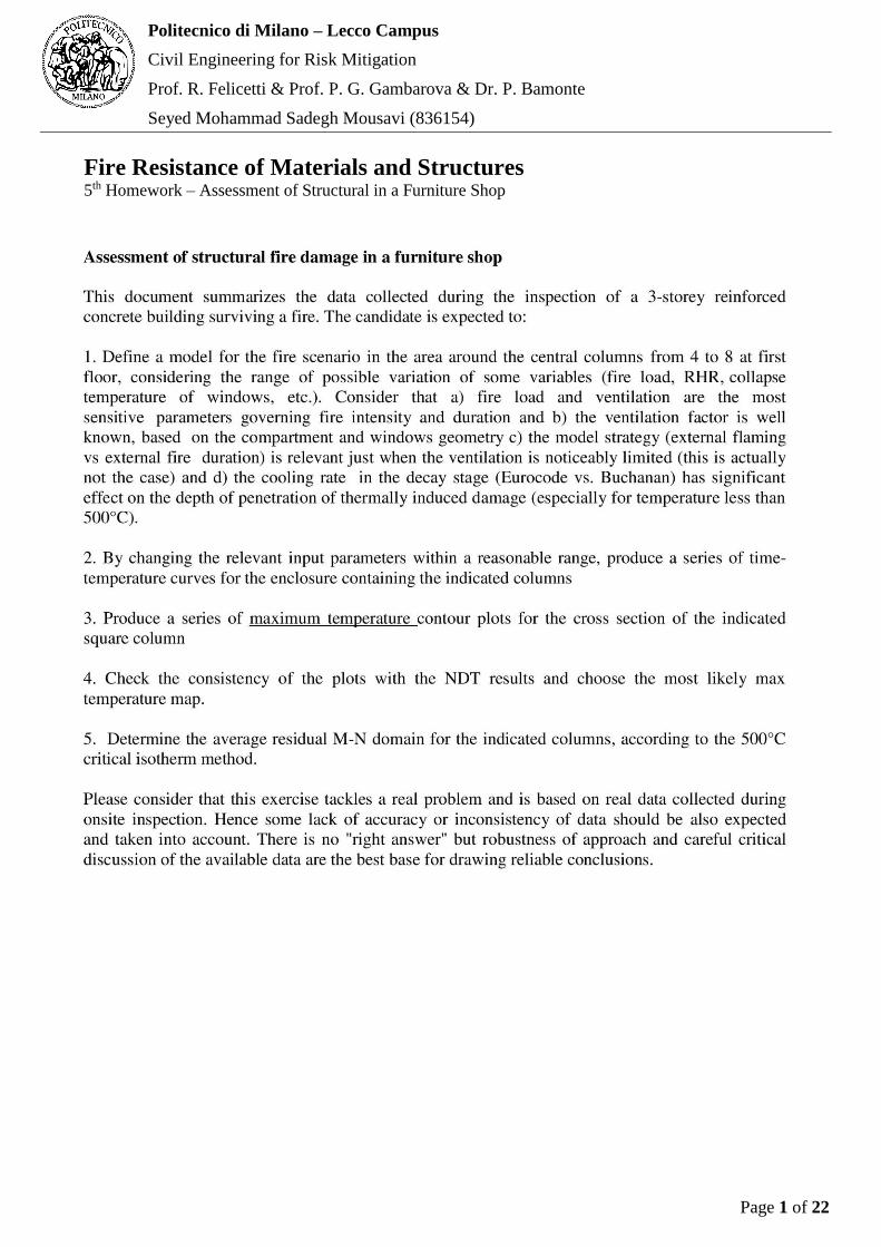
The results obtained are presented here in more detail. Table 4 shows the values given for the sensitivity

analysis of the concrete under study and the values obtained for the relative slowness of the damaged

concrete to the concrete unaffected. Figure 7 shows the curve that is fitted for the data. A third order

polynomial completely fits the data with a coefficient of determination equal to 1. As temperature gets

of 22





higher the relative slowness increases which means that in damaged concrete the waves have a higher

slowness, or in another word, it takes more time for them to go through the element.

Table 4-Refrence values for relative ultrasonic pulse velocity and slowness

T (°C) UPV (VT/V20) ST/S20

20 1 1

200 0.891 1.12

400 0.678 1.47

600 0.386 2.59

800 0.199 5.02

Figure 7- relationship between relative slowness and temperature

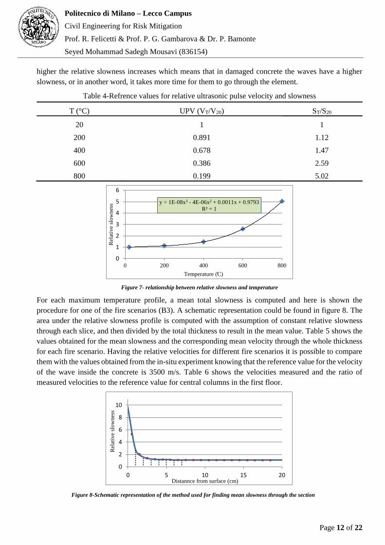
For each maximum temperature profile, a mean total slowness is computed and here is shown the

procedure for one of the fire scenarios (B3). A schematic representation could be found in figure 8. The

area under the relative slowness profile is computed with the assumption of constant relative slowness

through each slice, and then divided by the total thickness to result in the mean value. Table 5 shows the

values obtained for the mean slowness and the corresponding mean velocity through the whole thickness

for each fire scenario. Having the relative velocities for different fire scenarios it is possible to compare

them with the values obtained from the in-situ experiment knowing that the reference value for the velocity

of the wave inside the concrete is 3500 m/s. Table 6 shows the velocities measured and the ratio of

measured velocities to the reference value for central columns in the first floor.

Figure 8-Schematic representation of the method used for finding mean slowness through the section

y = 1E-08x3 - 4E-06x2 + 0.0011x + 0.9793

R² = 1

0

1

2

3

4

5

6

0 200 400 600 800

Rel

ativ

e sl

ow

nes

s

Temperature (C)

0

2

4

6

8

10

0 5 10 15 20

Rel

ativ

e sl

ow

nes

s

Distannce from surface (cm)

of 22





Table 5-meantotal slowness and velocity for different fire scenarios

Fire scenario A1 A2 A3 A4 A5 A6

A3

2 B1 B2 B3 B4 B5 B6 B32

mean

slowness

1.1

0

1.1

4

1.1

7

1.2

1

1.2

4

1.2

7

1.1

7

1.1

7

1.2

6

1.3

6

1.4

7

1.5

8

1.6

9

1.3

6

mean total

velocity

0.9

1

0.8

8

0.8

5

0.8

3

0.8

1

0.7

9

0.8

5

0.8

5

0.7

9

0.7

4

0.6

8

0.6

3

0.5

9

0.7

3

Table 6-relative ultrasonic pulse velocity values for central columns in the first floor

C1 C2 C4 C6 C8

UPV (m/s) 2997 3025 2696 3432 2736

Vel/Ref. vel. 85.6% 86.4% 77% 98.1% 78.2%

What is noteworthy in the results is the considerable difference between the relative velocity for the

column C6 and C8 while in the other experiments carried out the level of damage to this two columns are

estimated to be somewhat similar. A comparison with results acquired for other columns may come to the

conclusion that a 98.1% relative velocity for C6 is rather too high and appears to be affected by other

factors during the measurement. To support this idea, analogy is driven between central columns in the

first and second floor and a comparison is made between these two groups. As the ventilation is

comparable in these two floors (O = 0.09 e 0.06 respectively) it is expected that the damage incurred to

the structural elements would be also comparable (with the assumption of the same quality of concrete

before the fire). Table 7 shows the results for central columns in the second floor. It is interesting to see

that except for C6 in the first floor, the corresponding columns present a good correlation with each other

between first and second floor. The largest difference observed is for C4 between two floors which is less

than 10%. By this comparison it seems to be reasonable to disregard the 98.1% relative velocity of C6 in

the first floor.

Table 7-relative ultrasonic pulse velocity values for central columns in the second floor

C1 C4 C6 C7

UPV (m/s) 3140 3015 2804 2885

Vel/Ref. vel. 89.7% 86.1% 80.1 82.4

Based on the aforementioned, the focus will be on columns C4 and especially C8 in the first floor. Again,

column C4 is showing the poorest condition which confirms the assumption that due to higher ventilation

around this column higher temperatures were experienced and hence, higher extent of damage observed.

For column C8 a 78.2% relative velocity is reported which to be compared with fire scenarios seems to

match well with one of A5, A6, B2 or B3.

Another point that is worth mentioning is the comparison between the façade columns in the first and

second floor. Table 8 shows the results collected for these columns. The values for the first floor show a

sensible increase compared to the vales for the second floor. The reason may be related to the fact that

based on the sequence of the fire development in the building which is inferred from the images published,

the flashover occurs first in the second floor with a considerable external flaming and after that there is

the flashover in the first floor with some delay which, is also accompanied by external flaming. It could

be assumed that the external flaming in the first floor has not last long before the fire was put out and

of 22





hence the damage to the façade columns is much lower, some even not affected based on these results,

compared to the façade columns in the second floor which have undergone a longer fire duration and a

longer period of flashover. However, the results of rebound hammer, except for F1 and F2, does not

confirm this hypothesis and the only conclusion driven could be that the fire was not sever close to F1 and

F2 in the western side of the building.

Table 8-facade columns relative ultrasonic pulse velocity values for first and second floor

F1 F2 F4 F5 F6 F7 F8 F10

First 110% _ 90.6% _ 85.9% _ 100% 97.7%

Second _ 72.7% _ 85.9% _ 83.4%

Finally a general comparison between the results of UPV and Rebound hammer is made. Table 9 shows

the values obtained for different columns in both first and second floor for both nondestructive tests carried

out. Generally speaking not a clear relationship is evident between the values of UPV and Rebound

hammer index. For some columns UPV values are higher while for some others Rebound Indices are

higher and also in some columns close results are obtained.

Table 9- comparison between results obtained for UPV and Reb. tests

C1 C2 C4 C6 C8 (C7)

Reb. UPV Reb. UPV Reb. UPV Reb. UPV Reb. UPV

1st-C 79.6 85.6 77 86.4 77 77 88 98.1 90 78.2

2nd-C 77 89.7 - - 82 86.1 82 80.1

F2 F4 F6 (F5) F8 (F7) F10

1st-F 102 110 86 90.6 88 85.9 81 100 89 97.7

2nd-F 82 72.7 83 85.9 81 83.4

3-3- Indirect Ultrasonic Pulse Velocity Test

Indirect ultrasonic pulse velocity method is a good method for assessing the condition of the surface layer

of a damaged concrete as the wave does not propagate deep into the concrete and the results are mostly

affected by the surface layer properties. Here, the results pertaining to this test is presented. To assess the

depth of damage, the transducers are positioned on one side of the surface under study and the time of

travel of the ultrasonic wave is measured. This procedure is done for different distances between the

transducers and for each distance, X, and travel time T is measured. Measuring the time of arrival of the

wave may not be an easy and straightforward task as the onset of the receiving signal may not be readily

recognizable from the trail noise. Some methods exist for determination of the onset of an ultrasonic wave.

The approach adopted in this study is based on Akaike Information Criteria (AIC). Having pairs of X and

T, it is possible to plot T-X diagram. As the distance between the two transducers increases, the shortest

path for the wave to travel in the concrete switches from travelling only in a very shallow layer to a

compromise between shallow layers with shorter path and deeper layers with higher velocity. This

combined travel path is what advantage is taken form to comment on the degree of damage and

deterioration in concrete surface. The further the transducers get, the more contribution of the deeper

layers in transmitting the wave, and from a certain depth that the concrete is not considered to be damaged,

the travel velocity will be that of the healthy concrete which is taken as 3500 m/s. In the T-X plot, with

increasing X, travel velocity increases and therefore the slope of the plot being 1/V, decreases to a point

of 22





where V=V20, being V20 the wave travel velocity in pristine concrete. Changing the ordinates of this plot

to TV20 or in the other words, TVref, gives a curve in which the final slope equals 1. Extending the final

asymptote of this curve gives an intercept on TVref coordinate which is a measure of the damaged depth

of concrete. This is the thickness throughout which, the ultrasonic wave in damaged concrete has fallen

behind from an ultrasonic wave travelling with Vref. There are empirical relationships that for a specific

intercept of the TVref-X, give the depth of concrete in which the velocity of wave is lower than 80% of

the Vref. This depth which is considered to be the damaged depth corresponds to a 300 C isotherm. Beyond

this depth the concrete is assumed to be intact. Here the results for the indirect UPV carried out are

presented. The results of this section are for the two sets of test undertaken on column C8 in the first floor.

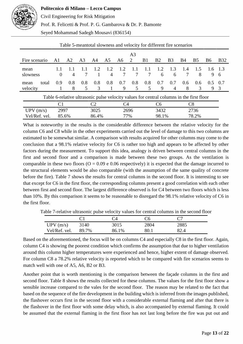
The TVref –X plot is shown in figure 9. Data recorded is also shown in table 10. The dotted line is the

extension of the final slope of the curve to intersect TVref coordinate. To obtain the plot, mean values of

the time of arrival are used. Furthermore, prior to working with the data acquired through the experiment,

the transducers were calibrated. Theoretically, if the distance between the transmitter and receiver is zero,

the time of travel should also equal zero, which means that the T-X plot should be a zero-intercept plot.

To adjust it, test were carried out beforehand using the same device on homogenous stone block plotting

T versus X. The intercept of this plot is found to be -12μsec with a slope of 0.361 μsec/mm. The probe

offset becomes 33.3 mm. This value should be added to the distance between probes.

Figure 9-TVref-X plot

Table 10-Data recorded for the indirect UPV test

0

100

200

300

400

500

600

700

800

0 100 200 300 400 500 600

TV

ref

Distance between transducers (mm)

Distance

(mm)

calibrated distance

(mm)

T1

arrival

T2

arrival Mean T

TmeanVref

200 233.3 97.163 97.146 97.15 340.04

250 283.3 115.54 107.24 111.39 389.86

300 333.3 139.74 133.55 136.64 478.25

350 383.3 157 135.75 146.37 512.31

400 433.3 161.55 166.62 164.08 574.29

450 483.3 191.36 185.88 188.62 660.17

500 533.3 207.15 200.93 204.04 714.14

550 583.3 207.15 207.18 207.16 725.07

600 633.3 207.13 207.18 207.15 725.04

of 22





To get a reasonable plot in which the final slope equals 1, the two last readings of both columns at X=

550 and 600mm, were excluded. As the probes get further from each other, the attenuation of the wave

amplitude increases which makes it more difficult to get reliable and accurate results for the time of arrival

of the receiving pulse, therefore, getting unreasonable results in the last readings is not far from

expectation. In so doing, the curve fitted to the readings showed a final slope of almost unity. The Intercept

of the extension of the final portion of the curve with TVref coordinate was then computed to be 180.84

mm.

An empirical formula proposed in [] which correlates the intercept to the layer of concrete undergone

discernible damage is 59log 233t X in which t (mm) is the thickness of a layer of concrete

corresponding to 300 C isotherm. According to the procedure adopted in this study, the damaged thickness

based on indirect ultrasonic test becomes 74mm. . Searching in the temperature profiles, it is found that

these results give a damage level higher than that any of the fire scenarios can justify. This is due the

degradation process that was described earlier. Although the rebound hammer also examines the quality

of a shallow layer of concrete, this phenomenon seems to be more reflected in the indirect ultrasonic pulse

velocity test.

3-4- Drilling Resistance

The drilling resistance test is carried out on 5 distinct points on column C4. The results are depicted in

figure 10. It is clear that as expected the values obtained have very high variation and oscillations.

Generally speaking, in all points there is first an increasing branch and afterwards the drilling resistance

measurements seem to be oscillating around a more or less constant value. In this region, concrete is

believed not to be affected by the fire and has its pristine condition.

of 22





Figure 10- Drilling resistance results for 5 different points on column C4

With the aim of assessing a point after which the concrete is assumed not to be affected by heat,

comparison is made between the data obtained from column C4 and the data from the reference column

from the same floor. To do so, the mean value of the drilling resistance for the reference column is obtained

with an 80% confidence level. The goodness of fit of the drilling resistance values with normal distribution

function is studied (figure 11 shows the plotting position). Although not a good accordance is observed

between the behavior of normal distribution function and drilling resistance data, it is chosen for the

purpose of a better scrutiny of the results.

Figure 11-plotting position for normal distribution for data obtained from drilling resistance test on the unaffected column

To be able to study better the results of column C4, the mean value of the drilling resistance measured in

all points is computed to eliminate some part of the variations. Moreover, using a 5 point method, the

curve is smoothed so that a clearer general behavior could be observed. Figure 12 shows the curve

0

10

20

30

40

50

60

0.0 10.0 20.0 30.0 40.0 50.0 60.0 70.0 80.0 90.0 100.0

dri

llin

g w

ork

(J/

mm

)

hole depth (mm)

point a

0

10

20

30

40

50

60

0.0 20.0 40.0 60.0 80.0 100.0

dri

llin

g w

ork

(J/

mm

)

hole depth (mm)

Point b

0

10

20

30

40

50

60

0.0 10.0 20.0 30.0 40.0 50.0 60.0 70.0 80.0 90.0 100.0

dri

llin

g w

ork

(J/

mm

)

hole depth (mm)

Point C

0

10

20

30

40

50

60

0.0 10.0 20.0 30.0 40.0 50.0 60.0 70.0 80.0 90.0 100.0

dri

llin

g w

ork

(J/

mm

)hole depth (mm)

Point e

0

10

20

30

40

50

60

0.0 10.0 20.0 30.0 40.0 50.0 60.0 70.0 80.0 90.0 100.0

dri

llin

g w

ork

(J/

mm

)

hole depth (mm)

Point d

0

10

20

30

40

50

60

70

-3 -2 -1 0 1 2 3

Dri

llin

g r

esis

tan

ce (

J/m

m)

Z (standard variable in normal distribution)

of 22





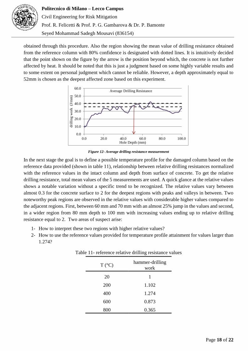
obtained through this procedure. Also the region showing the mean value of drilling resistance obtained

from the reference column with 80% confidence is designated with dotted lines. It is intuitively decided

that the point shown on the figure by the arrow is the position beyond which, the concrete is not further

affected by heat. It should be noted that this is just a judgment based on some highly variable results and

to some extent on personal judgment which cannot be reliable. However, a depth approximately equal to

52mm is chosen as the deepest affected zone based on this experiment.

Figure 12- Average drilling resistance measurement

In the next stage the goal is to define a possible temperature profile for the damaged column based on the

reference data provided (shown in table 11), relationship between relative drilling resistances normalized

with the reference values in the intact column and depth from surface of concrete. To get the relative

drilling resistance, total mean values of the 5 measurements are used. A quick glance at the relative values

shows a notable variation without a specific trend to be recognized. The relative values vary between

almost 0.3 for the concrete surface to 2 for the deepest regions with peaks and valleys in between. Two

noteworthy peak regions are observed in the relative values with considerable higher values compared to

the adjacent regions. First, between 60 mm and 70 mm with an almost 25% jump in the values and second,

in a wider region from 80 mm depth to 100 mm with increasing values ending up to relative drilling

resistance equal to 2. Two areas of suspect arise:

1- How to interpret these two regions with higher relative values?

2- How to use the reference values provided for temperature profile attainment for values larger than

1.274?

Table 11- reference relative drilling resistance values

T (°C) hammer-drilling

work

20 1

200 1.102

400 1.274

600 0.873

800 0.365

0.0

10.0

20.0

30.0

40.0

50.0

60.0

0.0 20.0 40.0 60.0 80.0 100.0

dri

llin

g w

ork

(J

/mm

)

Hole Depth (mm)

Average Drilling Resistance

of 22





To answer the first question, the two jumps in the results are distinguished, the first jump between 60 mm

to 70 mm and the second jump from 80 mm to the deepest layer under experiment. The first region has 1

cm thickness and the sudden jump could be attributed to the existence of a coarse aggregate oriented

exactly in the direction of the drilling which could be justified by the lower relative values both in deeper

and shallower depths before and after this region. The second region falls in the deepest layer under

examination and shows a clear increasing trend for a 2 cm thickness in the column. A reason could be that

this is the region beyond which (80 mm) concrete is not damaged by fire, in which case an increase in the

values is expected. This reasoning does not give the same results as the one obtained based on figure12

giving approximately 50 mm as the deepest damaged layer, yet, there is no clue favoring one justification

against the other. In fact what makes it even worse is that there is no good level of assurance over the

quality control of the concrete in time of construction, hence the remarkable higher drilling resistance

values obtained for a column under fire compared to an intact conrete could be easily because the concrete

cast in the column under fire had a greatly better quality from the beginning.

In either of the cases and with the aim of estimating a temperature profile and then to find the suitable fire

scenario, the approach that is taken is to disregard the outliers in both regions, from 60mm to 70mm and

from 80mm to 100mm, and by assuming a linear variation in temperatures given for the thermal sensitivity

of the concrete column. Although data is not provided for relative drilling resistance values over 1.274,

nonetheless if higher values could be taken as an indicative of lower temperatures, then it is assumed that

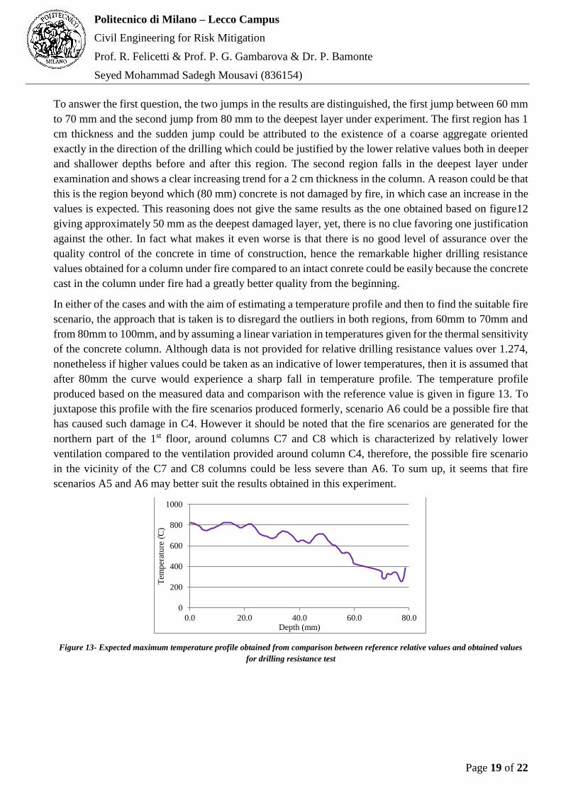
after 80mm the curve would experience a sharp fall in temperature profile. The temperature profile

produced based on the measured data and comparison with the reference value is given in figure 13. To

juxtapose this profile with the fire scenarios produced formerly, scenario A6 could be a possible fire that

has caused such damage in C4. However it should be noted that the fire scenarios are generated for the

northern part of the 1st floor, around columns C7 and C8 which is characterized by relatively lower

ventilation compared to the ventilation provided around column C4, therefore, the possible fire scenario

in the vicinity of the C7 and C8 columns could be less severe than A6. To sum up, it seems that fire

scenarios A5 and A6 may better suit the results obtained in this experiment.

Figure 13- Expected maximum temperature profile obtained from comparison between reference relative values and obtained values

for drilling resistance test

0

200

400

600

800

1000

0.0 20.0 40.0 60.0 80.0

Tem

per

atu

re (

C)

Depth (mm)

of 22





3-5- Carbonation Test

Results obtained for the depth of carbonation are shown in table 12. As is seen, the depth of carbonation

is the highest for C4 column in the first floor. Taking the depth of carbonation as the depth corresponding

to a temperature of 450 C, it is evident that based on these results the heat front has penetrated more in

C4 and that this column has undergone a more severe fire compared to C6 and C8. In the same manner

C6 is more damaged than C8. Results obtained from this experiment is in full agreement with other

experiments carried out demonstrating higher temperatures around column C4 and the lowest ventilation

around C8. Trying to find the best temperature profile matching these A5, A6 and B3 seem to be the

possible options.

Table 12- Obtained results for depth of carbonation

First floor Second floor

C4 21.2 F2 8.3

C6 20.8 C6a 15.5

C8 15.4 C6b 29.2

C7 13

3-6-Dynamic Hardness Test on Rebars

For the Leeb test as it is assumed that fy~ Leeb2, based on the leeb test done on site for a column away

from fire and the C4 column, it is concluded that fy,θ = 0.75fy,20. According to EC 3 - CEN EN1993-1-2,

the temperature corresponding to ky,θ = fy,θ / fy =0.75 is about 510 C. According to the geometry of the

columns with a cover of 20 mm, and based on the temperature profiles of the fire scenarios, the best

scenario matching this results would be B5 which experiences up to a temperature of 530 C at a 2 cm

depth from the surface of concrete.

4- Selection of a Fire Scenario

Going through the results acquired carrying out the nondestructive tests; it is possible to see that the

probable fire scenario to be selected for the unknown fire that occurred in the furniture shop would be the

A5 or A6, two of which are in good accordance with the results. A5 and A6 having a 600 and 700 MJ/m2

of fire loads and a rather medium fire growth rate with 90% of opening of all the openings from the outset

of the fire, are in higher consistency with the test results. Therefore, to produce an interaction domain for

the column under study, one of these two fire scenarios is chosen, A5.

5- M-N interaction domain of the column

The mean compressive strength of the concrete is considered to be around 20 MPa. This value was

obtained using the SonReb method and taking advantage of correlations developed between compressive

strength and these nondestructive testing. The result of a Leeb test method that was carried out on a part

of the structure that was away from the fire gave a value of about 330-350 Mpa for the reinforcing steel

that was used in the reinforced concrete. The column under study is a 4040 cm square with 8 14mm

rebars and a 2 cm cover. These information along with the 500 C isotherm of the A5 fire scenario are

used to determine the M-N interaction domain for the C4 column. To consider the mechanical decay of

concrete with temperature based on 500 C isotherm, the depth at which concrete temperature was equal

of 22





to 500 C was determined on the symmetry axis of the section. This depth was approximately 1.8 cm. .

Going further from the symmetry axis and approaching the corners of the section, this number will be

higher. With the aim of choosing a uniform depth beyond which concrete properties are assumed to be

intact, a 0.9 factor was used to result 1.8/0.9= 2cm. It was assumed that a 2cm thickness from the surface

of concrete was ineffective all around the column. Therefore it was possible to define a new column

section with dimensions of 3636 cm. Figure 15 shows the column geometry before the fire and the

equivalent cross section after the fire To assess the residual strength of the reinforcing bars, the concrete

temperature profile in a 2 cm depth from the surface is obtained from the outputs of the ABAQUS model.

Figure 14 shows this profile and the two squares are located in the position of the rebars for half of the

column with their corresponding temperature shown with the dotted lines. It is clear that the corner rebars

due to exposure to heat flux from two sides have higher temperatures.

Figure 14- Maximum temperature profile for a depth of 2cm parallel to the wall surface- location of rebars are shown with black marks

Having the maximum temperature profiles, it is easy to assess the maximum temperature that rebars have

experienced during the fire. Knowing the maximum temperature that rebars have experienced, it will be

possible to know their residual strength. Actually, during the cooling stage steel reinforcement recover to

some extent its mechanical properties and referring to the maximum temperature that reinforcements were

subjected to gives very conservative results for the computation of the residual resistance of a column. In

any case, this recovery effect is neglected in this study and the residual bearing capacity is estimated based

on the maximum temperature that reinforcing steel bars have undergone. Figure 15 shows the maximum

temperatures in each rebar. Due to the symmetry of the geometry and also the boundary conditions, the

corner rebars have the same maximum experienced temperature and the same condition exists for edge

rebars.

Figure 15- Column section before and after fire

200

300

400

500

600

700

800

900

0 1 2 3 4 5 6 7 8 9 10 11 12 13 14 15 16 17 18 19 20

Tem

per

atu

re (

C)

Distance along the wall (cm)

629 C

444 C

of 22





The Interaction diagram for the column before the fire occurrence is shown in figure 16. After fire the

mechanical properties decay and hence the interaction diagram tends to shrink.

Figure 16-Interaction diagram for the intact and damaged concrete

6- References

[1]- Eurocode 1: Actions on structures — Part 1-2: General actions — Actions on structures exposed to fire

[2]- Eurocode 2: Design of concrete structures — Part 1-2: General rules — Structural fire design

EN 1991-1-2 (2002), “Eurocode 1: Actions on structures. General actions - Actions on structures exposed to

fire”.

EN1992_1-2 (2004), “Eurocode 2: Design of concrete structures - Part 1-2: General rules - Structural fire

design”.

Bocca e Cianfrone (1983), “Le prove non distruttive sulle costruzioni: una metodologia combinata”, Industria

Italiana del Cemento, Vol. 6, p.429-436.

Felicetti R., Gambarova P.G. and Meda A. (2009), “Residual behaviour of stel rebars and R/C sections after

a fire”, Construction and Building Materials, V.23, N.12, p.3546-3555.

Felicetti R. (2009a), “Strutture in calcestruzzo armato: la valutazione del danno da incendio”, L’Edilizia -

Building and Construction for Engineers, V.17/159, pp.18-24.

Felicetti (2009b), “Strumenti per l’analisi del degrado nelle strutture in cls armato”, inbeton, n.58, p.46-55.

Felicetti R. (2011a), “Assessment Methods of Fire Damages in Concrete Tunnel Linings”, Fire Technology,

DOI 10.1007s10694-011-0229-6 (Online First publication).

Felicetti R. (2006), “The Drilling Resistance Test for the Assessment of Fire Damaged Concrete”, Journal of

Cement and Concrete Composites, V.28, p.321-329.

Felicetti R. (2011b), “Valutazione della resistenza residua delle armature esposte al fuoco”, Atti del 14°

Congresso AIPnD, Firenze, 26-28 ottobre, 8p.

-400

-200

0

200

400

600

800

1000

1200

1400

1600

1800

0 20 40 60 80 100

N (

KN

)

M (KN.m)

Residual

initial

fire resistance of materials & structures - assessment of structural in a furniture shop

Education