finite markov chains and algorithmic applicationsuosis.mif.vu.lt/~stepanauskas/mk/haggstrom o....
TRANSCRIPT

Finite Markov Chains and
Algorithmic Applications
OLLE H�GGSTR�M
London Mathematical SocietyStudent Texts 00

Finite Markov Chains and Algorithmic Applications

This Page Intentionally Left Blank

Finite Markov Chainsand
Algorithmic Applications
Olle HaggstromMatematisk statistik, Chalmers tekniska hogskola och Goteborgs universitet

PUBLISHED BY CAMBRIDGE UNIVERSITY PRESS (VIRTUAL PUBLISHING) FOR AND ON BEHALF OF THE PRESS SYNDICATE OF THE UNIVERSITY OF CAMBRIDGE The Pitt Building, Trumpington Street, Cambridge CB2 IRP 40 West 20th Street, New York, NY 10011-4211, USA 477 Williamstown Road, Port Melbourne, VIC 3207, Australia http://www.cambridge.org © Cambridge University Press 2002 This edition © Cambridge University Press (Virtual Publishing) 2003 First published in printed format 2002 A catalogue record for the original printed book is available from the British Library and from the Library of Congress Original ISBN 0 521 81357 3 hardback Original ISBN 0 521 89001 2 paperback ISBN 0 511 01941 6 virtual (netLibrary Edition)

Contents
Preface pagevii
1 Basics of probability theory 1
2 Markov chains 8
3 Computer simulation of Markov chains 17
4 Irreducible and aperiodic Markov chains 23
5 Stationary distributions 28
6 Reversible Markov chains 39
7 Markov chain Monte Carlo 45
8 Fast convergence of MCMC algorithms 54
9 Approximate counting 64
10 The Propp–Wilson algorithm 76
11 Sandwiching 84
12 Propp–Wilson with read-once randomness 93
13 Simulated annealing 99
14 Further reading 108
References 110Index 113
v

This Page Intentionally Left Blank

Preface
The first version of these lecture notes was composed for a last-year under-graduate course at Chalmers University of Technology, in the spring semester2000. I wrote a revised and expanded version for the same course one yearlater. This is the third and final (?) version.The notes are intended to be sufficiently self-contained that they can be read
without any supplementary material, by anyone who has previously taken (andpassed) some basic course in probability or mathematical statistics, plus someintroductory course in computer programming.The core material falls naturally into two parts: Chapters 2–6 on the basic
theory of Markov chains, and Chapters 7–13 on applications to a number ofrandomized algorithms.Markov chains are a class of random processes exhibiting a certain “mem-
oryless property”, and the study of these – sometimes referred to as Markovtheory – is one of the main areas in modern probability theory. This areacannot be avoided by a student aiming at learning how to design and implementrandomized algorithms, because Markov chains are a fundamental ingredientin the study of such algorithms. In fact, any randomized algorithm can (oftenfruitfully) be viewed as a Markov chain.I have chosen to restrict the discussion to discretetime Markov chains
with finite state space. One reason for doing so is that several of the mostimportant ideas and concepts in Markov theory arise already in this setting;these ideas are more digestible when they are not obscured by the additionaltechnicalities arising from continuous time and more general state spaces. Itcan also be argued that the setting with discrete time and finite state space isthe most natural when the ultimate goal is to construct algorithms: Discretetime is natural because computer programs operate in discrete steps. Finitestate space is natural because of the mere fact that a computer has a finiteamount of memory, and therefore can only be in a finite number of distinct
vii

viii Preface
“states”. Hence, the Markov chain corresponding to a randomized algorithmimplemented on a real computer has finite state space.However, I do not claim that more general Markov chains are irrelevant to
the study of randomized algorithms. For instance, an infinite state space issometimes useful as an approximation to (and easier to analyze than) a finitebut very large state space. For students wishing to dig into the more gen-eral Markov theory, the final chapter provides several suggestions for furtherreading.Randomized algorithms are simply algorithms that make use of random
number generators. In Chapters 7–13, the Markov theory developed in previ-ous chapters is applied to some specific randomized algorithms. The Markovchain Monte Carlo (MCMC) method, studied in Chapters 7 and 8, is a classof algorithms which provides one of the currently most popular methods forsimulating complicated stochastic systems. In Chapter 9, MCMC is appliedtothe problem of counting the number of objects in a complicated combinatorialset. Then, in Chapters 10–12, we study a recent improvement of standardMCMC, known as the Propp–Wilson algorithm. Finally, Chapter 13 deals withsimulated annealing, which is a widely used randomized algorithm for variousoptimization problems.It should be noted that the set of algorithms studied in Chapters 7–13
constitutes only a small (and not particularly representative) fractionof allrandomized algorithms. For a broader view of the wide variety of applicationsof randomization in algorithms, consult some of the suggestions for furtherreading in Chapter 14.The following diagram shows the structure of (essential) interdependence
between Chapters 2–13.
652 7
8 9
10
4
3
11
1213
How the chapters depend on each other.
Regarding exercises: Most chapters end with a number of problems. Theseare of greatly varying difficulty. To guide the student in the choice of problemsto work on, and the amount of time to invest into solving the problems, eachproblem has been equipped with a parenthesized number between(1) and

Preface ix
(10) to rank the approximate size and difficulty of the problem.(1) meansthat the problem amounts simply to checking some definition in the chapter (orsomething similar), and should be doable in a couple of minutes. At the otherend of the scale,(10) means that the problem requires a deep understandingof the material presented in the chapter, and at least several hours of work.Some of the problems require a bit of programming; this is indicated by anasterisk, as in(7*) .
� � � �
I am grateful to Sven Erick Alm, Nisse Dohrner, Devdatt Dubhashi, MihyunKang, DanMattsson, Jesper Møller and Jeff Steif, who all provided correctionsto and constructive criticism of earlier versions of this manuscript.

This Page Intentionally Left Blank

1
Basics of probability theory
The majority of readers will probably be best off by takingthe following pieceof advice:
Skip this chapter!
Those readers who have previously taken a basic course in probability ormathematical statistics will already know everything in this chapter, and shouldmove right on to Chapter 2. On the other hand, those readers who lack suchbackground will have little or no use for the telegraphic exposition givenhere, and should instead consult some introductory text on probability. Ratherthan being read, the present chapter is intended to be a collection of (mostly)definitions, that can be consulted if anything that looks unfamiliar happens toappear in the coming chapters.
� � � �
Let � be any set, and let� be some appropriate class of subsets of�,satisfying certain assumptions that we do not go further into (closedness undercertain basic set operations). Elements of� are calledevents. ForA ⊆ �, wewrite Ac for thecomplementof A in �, meaning that
Ac = {s ∈ � : s �∈ A} .
A probability measure on� is a functionP : � → [0,1], satisfying
(i) P(∅) = 0.(ii) P(Ac) = 1− P(A) for every eventA.(iii) If A andB are disjoint events (meaning thatA∩B = ∅), thenP(A∪B) =
P(A) + P(B). More generally, ifA1, A2, . . . is a countable sequence
1

2 1 Basics of probability theory
of disjoint events (Ai ∩ Aj = ∅ for all i �= j ), thenP(⋃∞
i=1 Ai) =∑∞
i=1P(Ai ).
Note that (i) and (ii) together imply thatP(�) = 1.If A and B are events, andP(B) > 0, then we define theconditional
probability of A given B, denotedP(A | B), as
P(A | B) = P(A∩ B)
P(B).
The intuitive interpretation ofP(A | B) is as how likely we consider the eventA to be, given that we know that the eventB has happened.Two eventsA andB are said to beindependentif P(A∩ B) = P(A)P(B).
More generally, the eventsA1, . . . , Ak are said to be independent if for anyl ≤ k and anyi1, . . . , i l ∈ {1, . . . , k} with i1 < i2 < · · · < i l we have
P(Ai1 ∩ Ai2 ∩ · · · ∩ Ail
) =l∏
n=1P(Ain) .
For an infinite sequence of events(A1, A2, . . .), we say thatA1, A2, . . . areindependent ifA1, . . . , Ak are independent for anyk.Note that ifP(B) > 0, then independence betweenA andB is equivalent
to havingP(A | B) = P(A), meaning intuitively that the occurrence ofB doesnot affect the likelihood ofA.A random variable should be thought of as some random quantity which
depends on chance. Usually a random variable is real-valued, in which case itis a functionX : � → R. We will, however, also consider random variablesin a more general sense, allowing them to be functionsX : � → S, whereScan be any set.An eventA is said to bedefined in terms of the random variableX if we
can read off whether or notA has happened from the value ofX. Examples ofevents defined in terms of the random variableX are
A = {X ≤ 4.7} = {ω ∈ � : X(ω) ≤ 4.7}and
B = {X is an even integer} .
Two random variables are said to be independent if it is the case that wheneverthe eventA is defined in terms ofX, and the eventB is defined in terms ofY,thenA andB are independent. IfX1, . . . , Xk are random variables, then theyare said to be independent ifA1, . . . , Ak are independent whenever eachAiis defined in terms ofXi . The extension to infinite sequences is similar: Therandom variablesX1, X2, . . . are said to be independent if for any sequence

Basics of probability theory 3
A1, A2, . . . of events such that for eachi , Ai is defined in terms ofXi , we havethatA1, A2, . . . are independent.A distribution is the same thing as a probability measure. IfX is a real-
valued random variable, then thedistribution µX of X is the probabilitymeasure onR satisfyingµX(A) = P(X ∈ A) for all (appropriate)A ⊆ R.The distribution of a real-valued random variable is characterized in terms ofits distribution function FX : R → [0,1] defined byFX(x) = P(X ≤ x) forall x ∈ R.A distributionµ on a finite setS = {s1, . . . , sk} is often represented as a
vector (µ1, . . . , µk), whereµi = µ(si ). By the definition of a probabilitymeasure, we then have thatµi ∈ [0,1] for eachi , and that∑k
i=1µi = 1.A sequence of random variablesX1, X2, . . . is said to bei.i.d., which is
short forindependent and identically distributed, if the random variables
(i) are independent, and
(ii) have the same distribution function, i.e.,P(Xi ≤ x) = P(X j ≤ x) for alli , j andx.
Very often, a sequence(X1, X2, . . .) is interpreted as the evolution in timeof some random quantity:Xn is the quantity at timen. Such a sequence is thencalled arandom process(or, sometimes,stochastic process). Markov chains,to be introduced in the next chapter, are a special class of random processes.We shall only be dealing with two kinds of real-valued random variables:
discreteandcontinuousrandom variables. The discrete ones take their valuesin some finite or countable subset ofR; in all our applications this subset is (oris contained in){0,1,2, . . .}, in which case we say that they arenonnegativeinteger-valueddiscrete random variables.A continuousrandom variableX is a random variable for which there exists
a so-calleddensity function fX : R → [0, ∞) such that∫ x
−∞fX(x)dx = FX(x) = P(X ≤ x)
for all x ∈ R. A very well-known example of a continuous random vari-able X arises by lettingX have the Gaussian density functionfX(x) =
1√2πσ2
e−((x−µ)2)/2σ2 with parametersµ andσ > 0. However, the only con-
tinuous random variables that will be considered in this text are theuniform[0,1] ones, which have density function
fX(x) ={1 if x ∈ [0,1]0 otherwise

4 1 Basics of probability theory
and distribution function
FX(x) =∫ x
−∞fX(x)dx =
0 if x ≤ 0x if x ∈ [0,1]1 if x ≥ 1 .
Intuitively, if X is a uniform [0,1] random variable, thenX is equally likelyto take its value anywhere in the unit interval [0,1]. More precisely, for everyinterval I of lengtha inside [0,1], we haveP(X ∈ I ) = a.Theexpectation(or expected value, ormean) E[X] of a real-valued ran-
dom variableX is, in some sense, the “average” value we expect fromx. If X isa continuous random variable with density functionfX(x), then its expectationis defined as
E[X] =∫ ∞
−∞x fX(x)dx
which in the case whereX is uniform [0,1] reduces to
E[X] =∫ 1
0x dx= 1
2.
For thecase whereX is a nonnegative integer-valued random variable, theexpectation is defined as
E[X] =∞∑k=1
kP(X = k) .
This can be shown to be equivalent to the alternative formula
E[X] =∞∑k=1
P(X ≥ k) . (1)
It is important to understand that the expectationE[X] of a random variablecan be infinite, even ifX itself only takes finite values. A famous example isthe following.
Example 1.1: The St Petersburg paradox.Consider the following game. Afair coin is tossed repeatedly until the first time that it comes up tails. LetX bethe (random) number of heads that come up before the first occurrence of tails.Suppose that the bank pays 2X roubles depending onX. How much would yoube willing to pay to enter this game?According to the classical theory of hazard games, you should agree to pay up
to E[Y], whereY = 2X is the amount that you receive from the bank at the endof the game. So let’s calculateE[Y]. We have
P(X = n) = P(n heads followed by 1 tail) =(1
2
)n+1

Basics of probability theory 5
for eachn, so that
E[Y] =∞∑k=1
kP(Y = k) =∞∑n=0
2nP(Y = 2n)
=∞∑n=0
2nP(X = n) =∞∑n=0
2n(1
2
)n+1
=∞∑n=0
1
2= ∞ .
Hence, there is obviously something wrong with the classical theory of hazardgames in this case.
Another important characteristic, besidesE[X], of a random variableX, is thevariance Var[X], defined by
Var [X] = E[(X − µ)2] whereµ = E[X] . (2)
The variance is, thus, the mean square deviation ofX from its expectation. Itcan be computed either using the defining formula (2), or by the identity
Var [X] = E[X2] − (E[X])2 (3)
known asSteiner’s formula.There are various linear-like rules for working with expectations and vari-
ances. For expectations, we have
E[X1 + · · · + Xn] = E[X1] + · · · + E[Xn] (4)
and, ifc is a constant,
E[cX] = cE[X] . (5)
For variances, we have
Var [cX] = c2Var [X] (6)
and,when X1, . . . , Xn are independent,1
Var [X1 + · · · + Xn] = Var [X1] + · · · + Var [Xn] . (7)
Let us compute expectations and variances in some simple cases.
Example 1.2Fix p ∈ [0,1], and let
X ={1 with probabilityp0 with probability 1− p .
1 Without this requirement, (7)fails in general.

6 1 Basics of probability theory
Such anX is called aBernoulli ( p) random variable. The expectation ofXbecomesE[X] = 0 · P(X = 0) + 1 · P(X = 1) = p. Furthermore, sinceX onlytakes the values 0 and 1, we haveX2 = X, so thatE[X2] = E[X], and
Var [X] = E[X2] − (E[X])2
= p− p2 = p(1− p)
using Steiner’s formula (3).
Example 1.3Let Y be the sum ofn independent Bernoulli (p) random variablesX1, . . . , Xn. (For instance,Y may be the number of heads inn tosses of a coinwith heads-probabilityp.) Such aY is said to be abinomial (n, p) randomvariable. Then, using (4) and (7), we get
E[Y] = E[X1] + · · · + E[Xn] = np
and
Var [Y] = Var [X1] + · · · + Var [Xn] = np(1− p) .
Variances are useful, e.g., for bounding the probability that a random variabledeviates by a large amount from its mean. We have, for instance, the followingwell-known result.
Theorem 1.1 (Chebyshev’s inequality)Let X be a random variable withmeanµ and varianceσ 2. For any a > 0, we have that the probabilityP[|X − µ| ≥ a] of a deviation from the mean of at least a, satisfies
P(|X − µ| ≥ a) ≤ σ 2
a2.
Proof Define another random variableY by setting
Y ={a2 if |X − µ| ≥ a0 otherwise.
Then we always haveY ≤ (X−µ)2, so thatE[Y] ≤ E[(X−µ)2]. Furthermore,E[Y] = a2P(|X − µ| ≥ a), so that
P(|X − µ| ≥ a) = E[Y]a2
≤ E[(X − µ)2]
a2
= Var [X]a2
= σ 2
a2.

Basics of probability theory 7
Chebyshev’s inequality will be used to prove a key result in Chapter 9(Lemma 9.3). A more famous application of Chebyshev’s inequality is in theproof of the following very famous and important result.
Theorem 1.2 (The Law of Large Numbers)Let X1, X2, . . . be i.i.d. randomvariables with finite meanµ and finite varianceσ 2. Let Mn denote the averageof the first n Xi ’s, i.e., Mn = 1
n(X1+ · · · + Xn). Then, for anyε > 0, we have
limn→∞P(|Mn − µ| ≥ ε) = 0 .
Proof Using (4) and (5) we get
E[Mn] = 1
n(µ + · · · + µ) = µ .
Similarly, (6) and (7) apply to show that
Var [Mn] = 1
n2(σ 2 + · · · + σ 2) = σ 2
n.
Hence, Chebyshev’s inequality gives
P(|Mn − µ| ≥ ε) ≤ σ 2
nε2
which tends to 0 asn → ∞.

2
Markov chains
Let us begin with a simple example. We consider a “random walker” in a verysmall town consisting of four streets, and four street-cornersv1, v2, v3 andv4
arranged as in Figure 1. At time 0, the random walker stands in cornerv1. Attime 1, he flips a fair coin and moves immediately tov2 or v4 according towhether the coin comes up heads ortails. At time 2, heflips the coin againto decide which of the two adjacent corners to move to, with the decision rulethat if the coin comes up heads, then he moves one step clockwise in Figure 1,while if it comes up tails, he moves one step counterclockwise. Thisprocedureis then iterated at times 3, 4,. . . .For eachn, let Xn denote the index of the street-corner at which the walker
stands at timen. Hence,(X0, X1, . . .) is a random process taking values in{1,2,3,4}. Since the walker starts at time 0 inv1, we have
P(X0 = 1) = 1 . (8)
Fig. 1. A random walker in a very small town.
8

Markov chains 9
Next, he will move tov2 or v4 with probability 12 each, so that
P(X1 = 2) = 1
2(9)
and
P(X1 = 4) = 1
2. (10)
To compute the distribution ofXn for n ≥ 2 requires a little more thought;you will be asked to do this in Problem2.1 below. To this end, it is useful toconsider conditional probabilities. Suppose that at timen, the walker standsat, say,v2. Then we get the conditional probabilities
P(Xn+1 = v1 | Xn = v2) = 1
2
and
P(Xn+1 = v3 | Xn = v2) = 1
2,
because of the coin-flipping mechanism for deciding where to go next. In fact,we get the same conditional probabilities if we condition further on the fullhistory of the process up to timen, i.e.,
P(Xn+1 = v1 | X0 = i0, X1 = i1, . . . , Xn−1 = in−1, Xn = v2) = 1
2
and
P(Xn+1 = v3 | X0 = i0, X1 = i1, . . . , Xn−1 = in−1, Xn = v2) = 1
2
for any choice ofi0, . . . , in−1. (This is because the coin flip at timen + 1is independent of all previous coin flips, and hence also independent ofX0, . . . , Xn.) This phenomenon is called thememoryless property, alsoknown as theMarkov property : the conditional distribution ofXn+1 given(X0, . . . , Xn) depends only onXn. Or in other words: to make the bestpossible prediction of what happens “tomorrow” (timen + 1), we only needto consider what happens “today” (timen), as the “past” (times 0, . . . ,n− 1)gives no additional useful information.2
Another interesting feature of this random process is that the conditionaldistribution ofXn+1 given thatXn = v2 (say) is the same for alln. (This isbecause the mechanism that the walker uses to decide where to go next is the
2 Please note that this is just a property of this particular mathematical model. It isnot intended asgeneral advice that we should “never worry about the past”. Of course, we have every reason,in daily life as well as in politics, to try to learn as much as we can from history in order tomake better decisions for the future!

10 2 Markov chains
same at all times.) This property is known astime homogeneity, or simplyhomogeneity.These observations call for a general definition:
Definition 2.1 Let P be a k× k matrix with elements{Pi, j : i, j = 1, . . . , k}.A random process(X0, X1, . . .) with finite state space S= {s1, . . . , sk} is saidto be a(homogeneous) Markov chain with transition matrix P, if for all n,all i , j ∈ {1, . . . , k} and all i0, . . . , in−1 ∈ {1, . . . , k} we have
P(Xn+1 = sj | X0 = si0, X1 = si1, . . . , Xn−1 = sin−1, Xn = si )
= P(Xn+1 = sj | Xn = si )
= Pi, j .
The elements of the transition matrixP are called transition probabilities. Thetransition probabilityPi, j is the conditional probability of being in statesj“tomorrow” given that we are in statesi “today”. The term “homogeneous” isoften dropped, and taken for granted when talking about “Markov chains”.For instance, the random walk example above is a Markov chain, with state
space{1, . . . ,4} and transition matrix
P =
0 1
2 0 12
12 0 1
2 00 1
2 0 12
12 0 1
2 0
. (11)
Every transition matrix satisfies
Pi, j ≥ 0 for all i, j ∈ {1, . . . , k} , (12)
andk∑j=1
Pi, j = 1 for all i ∈ {1, . . . , k} . (13)
Property (12) is just the fact that conditional probabilities are always nonneg-ative, and property (13) is that they sum to 1, i.e.,
P(Xn+1 = s1 | Xn = si ) + P(Xn+1 = s2 | Xn = si ) + · · ·+ P(Xn+1 = sk | Xn = si ) = 1 .
Wenext consider another important characteristic (besides the transitionma-trix) of a Markov chain(X0, X1, . . .), namely theinitial distribution , whichtells us how the Markov chain starts. The initial distribution is represented as
Markov chains 11
a row vectorµ(0) given by
µ(0) = (µ(0)1 , µ
(0)2 , . . . , µ
(0)k )
= (P(X0 = s1),P(X0 = s2), . . . ,P(X0 = sk)) .
Sinceµ(0) represents a probability distribution, we have
k∑i=1
µ(0)i = 1 .
In the random walk example above, we have
µ(0) = (1,0,0,0) (14)
because of (8).Similarly, we let the row vectorsµ(1), µ(2), . . . denote the distributions of
the Markov chain at times 1,2, . . . , so that
µ(n) = (µ(n)1 , µ
(n)2 , . . . , µ
(n)k )
= (P(Xn = s1),P(Xn = s2), . . . ,P(Xn = sk)) .
For the random walk example, equations (9) and (10) tell us that
µ(1) = (0, 12,0,12) .
It turns out that once we know the initial distributionµ(0) and the transitionmatrix P, we can compute all the distributionsµ(1), µ(2), . . . of the Markovchain. The following result tells us that this is simply a matter of matrixmultiplication. We writePn for thenth power of the matrixP.
Theorem 2.1For a Markov chain(X0, X1, . . .) with state space{s1, . . . , sk},initial distribution µ(0) and transition matrix P, we have for any n that thedistributionµ(n) at time n satisfies
µ(n) = µ(0)Pn . (15)
Proof Consider first the casen = 1. We get, forj = 1, . . . , k, that
µ(1)j = P(X1 = sj ) =
k∑i=1
P(X0 = si , X1 = sj )
=k∑i=1
P(X0 = si )P(X1 = sj | X0 = si )
=k∑i=1
µ(0)i Pi, j = (µ(0)P) j

12 2 Markov chains
where(µ(0)P) j denotes thej th element of the row vectorµ(0)P. Henceµ(1) =µ(0)P.To prove (15) for the general case, we use induction. Fixm, and suppose
that (15) holds forn = m. Forn = m+ 1, we get
µ(m+1)j = P(Xm+1 = sj ) =
k∑i=1
P(Xm = si , Xm+1 = sj )
=k∑i=1
P(Xm = si )P(Xm+1 = sj | Xm = si )
=k∑i=1
µ(m)i Pi, j = (µ(m)P) j
so thatµ(m+1) = µ(m)P. Butµ(m) = µ(0)Pm by the induction hypothesis, sothat
µ(m+1) = µ(m)P = µ(0)PmP = µ(0)Pm+1
and the proof is complete.
Let us consider some more examples – two small ones, and one huge:
Example 2.1: The Gothenburg weather.It is sometimes claimed that the bestway to predict tomorrow’s weather3 is simply to guess that it will be the sametomorrow as it is today. If we assume that this claim is correct,4 then it is naturalto model the weather asa Markov chain. For simplicity, we assume that there areonly two kinds of weather: rain and sunshine. If the above predictor is correct75% of the time (regardless of whether today’s weather is rain or sunshine), thenthe weather forms a Markov chain with state spaceS= {s1, s2} (with s1 = “rain”ands2 = “sunshine”) and transition matrix
P =[0.75 0.250.25 0.75
].
Example 2.2: The Los Angeles weather.Note that in Example 2.1, there is aperfect symmetry between “rain” and “sunshine”, in the sense that the probabilitythat today’s weather will persist tomorrow is the same regardless of today’sweather. This may be reasonably realistic in Gothenburg, but not in Los Angeleswhere sunshine is much more common than rain. A more reasonable transitionmatrix for the Los Angeles weather might therefore be (still withs1 = “rain” ands2 = “sunshine”)
P =[0.5 0.50.1 0.9
]. (16)
3 Better than watching the weather forecast on TV.4 I doubt it.

Markov chains 13
Example 2.3: The Internet as a Markov chain.Imagine that you are surfing onthe Internet, and that each time that you encounter a web page, you click on oneof its hyperlinks chosen at random (uniformly). IfXn denotes where you are aftern clicks, then(X0, X1, . . .) may be described as a Markov chain with state spaceSequal to the set of all web pages on the Internet, and transition matrixP givenby
Pi j ={
1di
if pagesi has a link to pagesj0 otherwise,
wheredi is the number of links from pagesi . (To make this chain well-defined,we also need to define what happens if there are no links at all fromsi . We may,for instance, setPii = 1 (andPi j = 0 for all i �= j ) in that case, meaning thatwhen you encounter a page with no links, you are stuck.) This is of course a verycomplicated Markov chain (especially compared to Examples 2.1 and 2.2), but ithas nevertheless turned out to be a useful model which under various simplifyingassumptions admits interesting analysis.5
A recent variant (see Faginet al. [Fa]) of this model is to take into accountalso the possibility to use “back buttons” in web browsers. However, the resultingprocess(X0, X1, . . .) is then no longer a Markov chain, since what happens whenthe back button is pressed depends not only on the present stateXn, but in generalalso onX0, . . . , Xn−1. Nevertheless, it turns out that this variant can be studiedby a number of techniques from the theory of Markov chains. We will not sayanything more about this model here.
A useful way to picture a Markov chain is its so-calledtransition graph . Thetransition graph consists of nodes representing the states of the Markov chain,and arrows between the nodes, representing transition probabilities. This ismost easily explained by just showing the transition graphs of the examplesconsidered so far. See Figure 2.In all examples above, as well as in Definition 2.1, the “rule” for obtaining
Xn+1 from Xn did not change with time. In some situations, it is morerealistic,or for other reasons more desirable,6 to let this rule change with time. Thisbrings us to the topic ofinhomogeneous Markov chains, and the followingdefinition,which generalizes Definition 2.1.
Definition 2.2 Let P(1), P(2), . . . be a sequence of k× k matrices, each ofwhich satisfies(12)and(13). A random process(X0, X1, . . .) with finite statespace S= {s1, . . . , sk} is said to be aninhomogeneous Markov chain withtransition matrices P(1), P(2), . . . , if for all n, all i , j ∈ {1, . . . , k} and all5 It may also seem like a very big Markov chain. However, the devoted reader will soon knowhow to carry out (not just in principle, but also in practice) computer simulations of muchbigger Markov chains – see, e.g., Problem 7.2.
6 Such as in the simulated annealing algorithms of Chapter 13.

14 2 Markov chains
rain sun
0.5
0.1
0.5 0.9
rain sun
0.5
0.5
0.5
0.5
0.5 0.50.5 0.5
0.25
0.25
0.75 0.751 2
4 3
Fig. 2. Transition graphs for the random walker in Figure 1, and for Examples 2.1 and2.2.
i0, . . . , in−1 ∈ {1, . . . , k} we have
P(Xn+1 = sj | X0 = si0,X1 = si1, . . . , Xn−1 = sin−1, Xn = si )
= P(Xn+1 = sj | Xn = si )
= P(n+1)i, j .
Example 2.4: A refined model for the Gothenburg weather. There are ofcourse many ways in which the crude model in Example 2.1 can be made morerealistic. One way is to take into account seasonal changes: it does not seemreasonable to disregard whether the calendar says “January” or “July” when pre-dicting tomorrow’s weather. To this end, we extend the state space to{s1, s2, s3},wheres1 = “rain” ands2 = “sunshine” as before, ands3 = “snow”. Let
Psummer= 0.75 0.25 00.25 0.75 00.5 0.5 0
and Pwinter =
0.5 0.3 0.20.15 0.7 0.150.2 0.3 0.5
,
and assume that the weather evolves according toPsummerin May–September,and according toPwinter in October–April. This is an inhomogeneous Markovchain model for the Gothenburg weather. Note that in May–September, the modelbehaves exactly like the one in Example 2.1, except for some possible residualsnowy weather on May 1.
The following result, which is a generalization of Theorem 2.1, tells us howto compute the distributionsµ(1), µ(2), . . . at times 1,2, . . . of an inhomo-geneous Markov chain with initial distributionµ(0) and transition matricesP(1), P(2), . . . .
Theorem 2.2Suppose that(X0, X1, . . .) is an inhomogeneous Markov chainwith state space{s1, . . . , sk}, initial distribution µ(0) and transition matrices
Markov chains 15
P(1), P(2), . . . . For any n, we then have that
µ(n) = µ(0)P(1)P(2) · · · P(n) .
Proof Follows by a similar calculation as in the proof of Theorem 2.1.
Problems2.1 (5) Consider the Markov chain corresponding to the random walker in Figure 1,
with transition matrixP and initial distributionµ(0) given by (11) and (14).
(a) Compute the squareP2 of the transition matrixP. How can we interpretP2?(See Theorem 2.1, or glance ahead at Problem 2.5.)
(b) Prove by induction that
µ(n) ={
(0, 12,0,12) for n = 1,3,5, . . .
(12,0,12,0) for n = 2,4,6, . . . .
2.2 (2) Suppose that we modify the random walk example in Figure 1 as follows. Ateach integer time, the random walker tossestwo coins. The first coin is to decidewhether to stay or go. If it comes up heads, he stays where he is, whereas if itcomes up tails, he lets the second coin decide whether he should move one stepclockwise, or one step counterclockwise. Write down the transition matrix, anddraw the transition graph, for this new Markov chain.
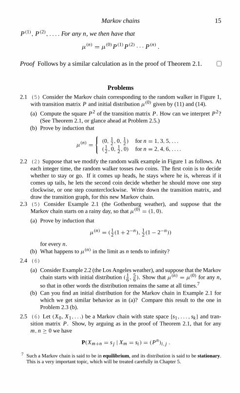
2.3 (5) Consider Example 2.1 (the Gothenburg weather), and suppose that theMarkov chain starts on a rainy day, so thatµ(0) = (1,0).
(a) Prove by induction that
µ(n) = (12(1+ 2−n), 12(1− 2−n))
for everyn.(b) What happens toµ(n) in the limit asn tends to infinity?
2.4 (6)
(a) Consider Example 2.2 (the Los Angeles weather), and suppose that theMarkovchain starts with initial distribution(16,
56). Show thatµ
(n) = µ(0) for anyn,
so that in other words the distribution remains the same at all times.7
(b) Can you find an initial distribution for the Markov chain in Example 2.1 forwhich we get similar behavior as in (a)? Compare this result to the one inProblem 2.3 (b).
2.5 (6) Let (X0, X1, . . .) be a Markov chain with state space{s1, . . . , sk} and tran-sition matrix P. Show, by arguing as in the proof of Theorem 2.1, that for anym,n ≥ 0 we have
P(Xm+n = sj | Xm = si ) = (Pn)i, j .
7 Such a Markov chain is said to be inequilibrium , and its distribution is said to bestationary.This is a very important topic, which will be treated carefully in Chapter 5.

16 2 Markov chains
2.6 (8) Functions of Markov chains are not always Markov chains. Let(X0, X1, . . .) be a Markov chain with state space{s1, s2, s3}, transition matrix
P = 0 1 00 0 11 0 0
and initial distributionµ(0) = (13,13,13). For eachn, define
Yn ={0 if Xn = s11 otherwise.
Show that(Y0,Y1, . . .) is nota Markov chain.2.7 (9) Markov chains sampled at regular intervals are Markov chains. Let
(X0, X1, . . .) be a Markov chain with transition matrixP.
(a) Define(Y0,Y1, . . .) by settingYn = X2n for eachn. Show that(Y0,Y1, . . .)is a Markov chain with transition matrixP2.
(b) Find an appropriate generalization of the result in (a) to the situation where wesample everykth (rather than every second) value of(X0, X1, . . .).

3
Computer simulation of Markov chains
A key matter in many (most?) practical applications of Markov theory is theability to simulate Markov chains on a computer. This chapter deals with howthat can be done.We begin by stating a lie:
In most high-level programming languages, we have access to some ran-dom number generator producing a sequenceU0,U1, . . . of i.i.d. randomvariables, uniformly distributed on the unit interval [0,1].
This is a lie for at least two reasons:
(A) The numbersU0,U1, . . . obtained from random number generators arenot uniformly distributed on [0,1]. Typically, they have a finite binary (ordecimal) expansion, and are therefore rational. In contrast, it can be shownthat a random variable which (truly) is uniformly distributed on [0,1] (orin fact any continuous random variable) is irrational with probability 1.
(B) U0,U1, . . . are not even random! Rather, they are obtained by somedeterministic procedure. For this reason, random number generators aresometimes (and more accurately) called pseudo-random number genera-tors.8
The most important of these objections is (B), because (A) tends not to be avery big problem when the number of binary or decimal digits is reasonablylarge (say, 32 bits). Over the decades, a lot of effort has been put into construct-ing (pseudo-)random number generators whose output is as indistinguishable
8 There are also various physically generated sequences of random-looking numbers (see,e.g., the web siteshttp://lavarand.sgi.com/ and http://www.fourmilab.ch/hotbits/ ) that may be used instead of the usual pseudo-random number generators.I recommend, however, a healthy dose of skepticism towards claims that these sequences arein some sense “truly” random.
17

18 3 Computer simulation of Markov chains
as possible from a true i.i.d. sequence of uniform [0,1] random variables.Today, there exist generators which appear to do this very well (passing all ofa number of standard statistical tests for such generators), and for this reason,we shall simply make the (incorrect) assumption that we have access to ani.i.d. sequence of uniform[0,1] random variables U0,U1, . . . . Although weshall not deal any further with the pseudo-randomness issue in the remainderof these notes (except for providing a coupleof relevant references in thefinalchapter), we should always keep in mind that it is a potential source of errorsin computer simulation.9
Let us move on to the core topic of this chapter: How do we simulate aMarkov chain(X0, X1, . . .) with given state spaceS = {s1, . . . , sk}, initialdistributionµ(0) and transition matrixP? As the reader probably has guessedby now, the random numbersU0,U1, . . . form a main ingredient. The othermain ingredients are two functions, which we call theinitiation function andtheupdate function.The initiation functionψ : [0,1] → S is a function from the unit interval to
the state spaceS, which we use to generate the starting valueX0. We assume
(i) thatψ is piecewise constant (i.e., that [0,1] can be split into finitely manysubintervals in such a way thatψ is constant on each interval), and
(ii) that for eachs ∈ S, the total length of the intervals on whichψ(x) = sequalsµ(0)(s).
Another way to state property (ii) is that∫ 1
0I {ψ(x)=s} dx = µ(0)(s) (17)
for eachs ∈ S; hereI {ψ(x)=s} is the so-calledindicator function of {ψ(x) =s}, meaning that
I {ψ(x)=s} ={1 if ψ(x) = s0 otherwise.
Provided that we have such a functionψ , we can generateX0 from the firstrandom numberU0 by settingX0 = ψ(U0). This gives the correct distributionof X0, because for anys ∈ Swe get
P(X0 = s) = P(ψ(U0) = s) =∫ 1
0I {ψ(x)=s} dx = µ(0)(s)
9 A misunderstanding that I have encountered more than once is that a pseudo-random numbergenerator is good if its period (the time until it repeats itself) is long, i.e., longer than the numberof random numbers needed in a particular application. But this is far from sufficient, and manyother things can go wrong. For instance, certain patterns may occur too frequently (or all thetime).

Computer simulation of Markov chains 19
using (17). Hence, we callψ a valid initiation function for the Markov chain(X0, X1, . . .) if (17) holds for alls ∈ S.Valid initiation functions are easy to construct: WithS = {s1, . . . , sk} and
initial distributionµ(0), we can set
ψ(x) =
s1 for x ∈ [0, µ(0)(s1))
s2 for x ∈ [µ(0)(s1), µ(0)(s1) + µ(0)(s2))
......
si for x ∈[∑i−1
j=1µ(0)(sj ),∑i
j=1µ(0)(sj ))
......
sk for x ∈[∑k−1
j=1µ(0)(sj ), 1].
(18)
We need to verify that this choice ofψ satisfies properties (i) and (ii) above.Property (i) is obvious. As to property (ii), it suffices to check that (17) holds.It does hold, since
∫ 1
0I {ψ(x)=si } dx =
i∑j=1
µ(0)(sj ) −i−1∑j=1
µ(0)(sj ) = µ(0)(si )
for i = 1, . . . , k. This means thatψ as defined in (18) is a valid initiationfunction for the Markov chain(X0, X1, . . .).So now we know how to generate the starting valueX0. If we also figure
out how to generateXn+1 from Xn for anyn, then we can use this procedureiteratively to get the whole chain(X0, X1, . . .). To get fromXn to Xn+1, weuse the random numberUn+1 and anupdate function φ : S× [0,1] → S,which takes as input a states ∈ Sand a number between 0 and 1, and producesanother states′ ∈ S as output. Similarly as for the initiation functionψ , weneedφ to obey certain properties, namely
(i) that for fixedsi , the functionφ(si , x) is piecewise constant (when viewedas a function ofx), and
(ii) that for each fixedsi , sj ∈ S, the total length of the intervals on whichφ(si , x) = sj equalsPi, j .
Again, as for the initiation function, property (ii) can be rewritten as
∫ 1
0I {φ(si ,x)=sj } dx = Pi, j (19)

20 3 Computer simulation of Markov chains
for all si , sj ∈ S. If the update functionφ satisfies (19), then
P(Xn+1 = sj | Xn = si ) = P(φ(si ,Un+1) = sj | Xn = si ) (20)
= P(φ(si ,Un+1) = sj )
=∫ 1
0I {φ(si ,x)=sj } dx = Pi, j .
The reason that the conditioning in (20) can be dropped is thatUn+1 is inde-pendent of(U0, . . . ,Un), and hence also ofXn. The same argument showsthat the conditional probability remains the same if we condition further onthe values(X0, X1, . . . , Xn−1). Hence, this gives a correct simulation of theMarkov chain. A functionφ satisfying (19) is therefore said to be a validupdate function for the Markov chain(X0, X1, . . .).It remains to construct such a valid update function, but this is no harder
than the construction of a valid initiation function: Set, for eachsi ∈ S,
φ(si , x) =
s1 for x ∈ [0, Pi,1)s2 for x ∈ [Pi,1, Pi,1 + Pi,2)...
...
sj for x ∈[∑ j−1
l=1 Pi,l ,∑ j
l=1 Pi,l)
......
sk for x ∈[∑k−1
l=1 Pi,l , 1].
(21)
To see that this is a valid update function, note that for anysi , sj ∈ S, we have
∫ 1
0I {φ(si ,x)=sj } dx =
j∑l=1
Pi,l −j−1∑l=1
Pi,l = Pi, j .
Thus, we have a complete recipe for simulating a Markov chain: Firstconstruct valid initiation and update functionsψ andφ (for instance as in (18)and (21)), and then set
X0 = ψ(U0)
X1 = φ(X0,U1)
X2 = φ(X1,U2)
X3 = φ(X2,U3)
and so on.Let us now see how the above works for a simple example.
Example 3.1: Simulating the Gothenburg weather.Consider the Markov chainin Example 2.1, whose state space isS = {s1, s2} wheres1 = “rain” and s2 =

Computer simulation of Markov chains 21
“sunshine”, and whose transition matrix is given by
P =[0.75 0.250.25 0.75
].
Suppose we start the Markov chain on a rainy day (as in Problem 2.3), so thatµ(0) = (1,0). To simulate this Markov chain using the above scheme, we apply(18) and (21) to get the initiation function
ψ(x) = s1 for all x ,
and update function given by
φ(s1, x) ={s1 for x ∈ [0,0.75)s2 for x ∈ [0.75,1]
and
φ(s2, x) ={s1 for x ∈ [0,0.25)s2 for x ∈ [0.25,1] . (22)
Before closing this chapter, let us finally point out how the above methodcan be generalized to cope with simulation of inhomogeneous Markov chains.Let (X0, X1, . . .) be an inhomogeneous Markov chain with state spaceS ={s1, . . . , sk}, initial distributionµ(0), and transition matricesP(0), P(1), . . . .
We can then obtain the initiation functionψ and the starting valueX0 as inthe homogeneous case. The updating is done similarly as in the homogeneouscase, except that since the chain is inhomogeneous, we need several differentupdating functionsφ(1), φ(2), . . . , and for these we need to have
∫ 1
0I {φ(n)(si ,x)=sj }(x)dx = P(n)
i, j
for eachn and eachsi , sj ∈ S. Such functions can be obtained by the obviousgeneralization of (21): Set
φ(n)(si , x) =
s1 for x ∈ [0, P(n)i,1 )
s2 for x ∈ [P(n)i,1 , P(n)
i,1 + P(n)i,2 )
......
sj for x ∈[∑ j−1
l=1 P(n)i,l ,
∑ jl=1 P
(n)i,l
)...
...
sk for x ∈[∑k−1
l=1 P(n)i,l , 1
].

22 3 Computer simulation of Markov chains
The inhomogeneous Markov chain is then simulated by setting
X0 = ψ(U0)
X1 = φ(1)(X0,U1)
X2 = φ(2)(X1,U2)
X3 = φ(3)(X2,U3)
and so on.
Problems3.1 (7*)
(a) Find valid initiation and update functions for the Markov chain in Example 2.2(the Los Angeles weather), with starting distributionµ(0) = (12,
12).
(b) Write a computer program for simulating theMarkov chain, using the initiationand update functions in (a).
(c) Forn ≥ 1, defineYn to be the proportion of rainy days up to timen, i.e.,
Yn = 1
n+ 1
n∑i=0
I {Xi=s1} .
Simulate the Markov chain for (say) 1000 steps, and plot howYn evolveswith time. What seems to happen toYn whenn gets large? (Compare withProblem 2.4 (a).)
3.2 (3) The choice of update function is not necessarily unique.Consider Ex-ample 3.1 (simulating the Gothenburg weather). Show that we get another validupdate function if we replace (22) by
φ(s2, x) ={s2 for x ∈ [0,0.75)s1 for x ∈ [0.75,1] .

4
Irreducible and aperiodic Markov chains
For several of the most interesting results in Markov theory, we need to putcertain assumptions on the Markov chains we are considering.It is an impor-tant task, in Markov theory just as in all other branches of mathematics, to findconditions that on the one hand arestrong enough to have useful consequences,but on the other hand are weak enough to hold (and be easy to check) for manyinteresting examples. In this chapter, we will discuss two such conditionson Markov chains:irreducibility andaperiodicity. Theseconditions are ofcentral importance in Markov theory, and in particular they play a key role inthe study of stationary distributions, which is the topic of Chapter 5. We shall,for simplicity, discuss these notions in the setting of homogeneous Markovchains, although they do have natural extensions to the more general setting ofinhomogeneous Markov chains.We begin with irreducibility, which, loosely speaking, is the property that
“all states of the Markov chain can be reached from all others”. To makethis more precise, consider a Markov chain(X0, X1, . . .) with state spaceS={s1, . . . , sk} and transition matrixP. We say that a statesi communicateswithanother statesj , writing si → sj , if the chain has positive probability10 of everreachingsj when we start fromsi . In other words,si communicates withsj ifthere exists ann such that
P(Xm+n = sj | Xm = si ) > 0 .
By Problem 2.5, this probability is independent ofm (due to the homogeneityof the Markov chain), and equals(Pn)i, j .If si → sj andsj → si , then we say that the statessi andsj intercommuni-
cate, and writesi ↔ sj . This takes us directly to the definition of irreducibility.
10 Here and henceforth, by “positive probability”, we always meanstrictly positive probability.
23

24 4 Irreducible and aperiodic Markov chains
3 4
0.8
0.8
0.20.2
0.5
1 20.3
0.5 0.7
Fig. 3. Transition graph for the Markov chain in Example 4.1.
Definition 4.1AMarkov chain(X0, X1, . . .) with state space S= {s1, . . . , sk}and transition matrix P is said to beirreducible if for all si , sj ∈ S we havethat si ↔ sj . Otherwise the chain is said to bereducible.
Another way of phrasing the definition would be to say that the chain isirreducible if for anysi , sj ∈ Swe can find ann such that(Pn)i, j > 0.An easy way to verify that a Markov chain is irreducible is to look at
its transition graph, and check that from each state there is a sequence ofarrows leading to any other state. A glance at Figure 2 thus reveals that theMarkov chains in Examples 2.1and 2.2, as well as the random walk examplein Figure 1, are all irreducible.11 Let us next have a look at an example whichis not irreducible:
Example 4.1: A reducible Markov chain. Consider a Markov chain(X0, X1, . . .) with state spaceS= {1,2,3,4} and transition matrix
P =
0.5 0.5 0 00.3 0.7 0 00 0 0.2 0.80 0 0.8 0.2
.
By taking a look at its transition graph (see Figure 3), weimmediately see that ifthe chain starts in state 1 or state 2, then it is restricted to states 1 and 2 forever.Similarly, if it starts in state 3 or state 4, then it can never leave the subset{3,4}of the state space. Hence, the chain is reducible.
Note that if the chain starts in state 1 or state 2, then it behaves exactly as if itwere a Markov chain with state space{1,2} and transition matrix[
0.5 0.50.3 0.7
].
If it starts in state 3 or state 4, then it behaves like a Markov chain with state space
11 Some care is still needed; see Problem 4.1.

Irreducible and aperiodic Markov chains 25
{3,4} and transition matrix [0.2 0.80.8 0.2
].
This illustrates a characteristic feature of reducible Markov chains, which alsoexplains the term “reducible”: If a Markov chain is reducible, then the analysis ofits long-term behavior can be reduced to the analysis of the long-term behavior ofone or more Markov chains with smaller state space.
We move on to consider the concept of aperiodicity. For a finite or infiniteset{a1,a2, . . .} of positive integers, we write gcd{a1,a2, . . .} for the greatestcommon divisor ofa1,a2, . . . . Theperiod d(si ) of a statesi ∈ S is defined as
d(si ) = gcd{n ≥ 1 : (Pn)i,i > 0} .
In words, the period ofsi is the greatest common divisor of the set of times thatthe chain can return (i.e., has positive probability of returning) tosi , given thatwe start withX0 = si . If d(si ) = 1, then we say that the statesi is aperiodic.
Definition 4.2 A Markov chain is said to beaperiodic if all its states areaperiodic. Otherwise the chain is said to beperiodic.
Consider for instance Example 2.1 (the Gothenburg weather). It is easy tocheck that regardless of whether the weather today is rain or sunshine, wehave for anyn that the probability of having the same weathern days lateris strictly positive. Or, expressed more compactly:(Pn)i,i > 0 for all n andall statessi .12 This obviously implies that the Markov chain in Example 2.1is aperiodic. Of course, the same reasoning applies to Example 2.2 (the LosAngeles weather).On the other hand, let us consider the random walk example in Figure 1,
where the random walker stands in cornerv1 at time 0. Clearly, he has to takean even number of steps in order to get back tov1. This means that(Pn)1,1 > 0only for n = 2,4,6, . . . . Hence,
gcd{n ≥ 1 : (Pn)i,i > 0} = gcd{2,4,6, . . .} = 2 ,
and the chain is therefore periodic.One reason for the usefulness of aperiodicity is the following result.
Theorem 4.1Suppose that we have an aperiodic Markov chain(X0, X1, . . .)with state space S= {s1, . . . , sk} and transition matrix P. Then there existsan N< ∞ such that
(Pn)i,i > 0
12 By a variant of Problem 2.3 (a), we in fact have that(Pn)i,i = 12(1+ 2−n).

26 4 Irreducible and aperiodic Markov chains
for all i ∈ {1, . . . , k} and all n≥ N.
To prove this result, we shall borrow the following lemma from number theory.
Lemma 4.1Let A= {a1,a2, . . .} be a set of positive integers which is(i) nonlattice, meaning thatgcd{a1,a2, . . .} = 1, and
(ii) closed under addition, meaning that if a∈ A and a′ ∈ A, then a+a′ ∈ A.
Then there exists an integer N< ∞ such that n∈ A for all n ≥ N.
Proof See, e.g., the appendix of Bremaud [B].
Proof of Theorem 4.1For si ∈ S, let Ai = {n ≥ 1 : (Pn)i,i > 0}, so thatin other wordsAi is the set of possible return times to statesi starting fromsi . We assumed that the Markov chain is aperiodic, and therefore the statesiis aperiodic, so thatAi is nonlattice. Furthermore,Ai is closed under addition,for the following reason: Ifa,a′ ∈ Ai , thenP(Xa = si | X0 = si ) > 0 andP(Xa+a′ = si | Xa = si ) > 0. This implies that
P(Xa+a′ = si | X0 = si ) ≥ P(Xa = si , Xa+a′ = si | X0 = si )
= P(Xa = si | X0 = si )P(Xa+a′ = si | Xa = si )
> 0
so thata+ a′ ∈ Ai .
In summary,Ai satisfies assumptions (i) and (ii) of Lemma 4.1, whichtherefore implies that there exists an integerNi < ∞ such that(Pn)i,i > 0 forall n ≥ Ni .
Theorem 4.1 now follows withN = max{N1, . . . , Nk}.
By combining aperiodicity and irreducibility, we get the following importantresult, which will be used in the next chapter to prove the so-called Markovchain convergence theorem (Theorem5.2).
Corollary 4.1 Let (X0, X1, . . .) be an irreducible and aperiodic Markov chainwith state space S= {s1, . . . , sk} and transition matrix P. Then there existsan M < ∞ such that(Pn)i, j > 0 for all i , j ∈ {1, . . . , k} and all n≥ M.
Proof By the assumed aperiodicity and Theorem 4.1, there exists an integerN < ∞ such that(Pn)i,i > 0 for all i ∈ {1, . . . , k} and alln ≥ N. Fix twostatessi , sj ∈ S. By the assumed irreducibility, we can find someni, j such

Irreducible and aperiodic Markov chains 27
that(Pni, j )i, j > 0. LetMi, j = N + ni, j . For anym≥ Mi, j , we have
P(Xm= sj | X0= si ) ≥ P(Xm−ni, j = si , Xm= sj | X0= si )
= P(Xm−ni, j = si | X0= si )P(Xm= sj | Xm−ni, j = si )
> 0 (23)
(the first factor in the second line of (23) is positive becausem− ni, j ≥ N,and the second is positive by the choice ofni, j ). Hence, we have shown that(Pm)i, j > 0 for allm≥ Mi, j . The corollary now follows with
M = max{M1,1,M1,2 . . . ,M1,k,M2,1, . . . ,Mk,k} .
Problems4.1 (3) Consider the Markov chain(X0, X1, . . .) with state spaceS = {s1, s2} and
transition matrix
P =[ 1
212
0 1
].
(a) Draw the transition graph of this Markov chain.(b) Show that the Markov chain isnot irreducible (even though the transition
matrix looks in some sense connected).(c) What happens toXn in the limit asn → ∞?
4.2 (3) Show that if a Markov chain is irreducible and has a statesi such thatPii > 0,then it is also aperiodic.
4.3 (4) Random chess moves.
(a) Consider a chessboard with a lone white king making randommoves, meaningthat at each move, he picks one of the possible squares to move to, uniformlyat random. Is the corresponding Markov chain irreducible and/or aperiodic?
(b) Same question, but with the king replaced by a bishop.(c) Same question, but instead with a knight.
4.4 (6) Oriented random walk on a torus. Let a andb be positive integers, andconsider the Markov chain with state space
{(x, y) : x ∈ {0, . . . ,a− 1}, y ∈ {0, . . . ,b− 1}} ,
and the following transitionmechanism: If the chain is in state(x, y) at timen, thenat timen+ 1 it moves to((x+ 1)moda, y) or (x, (y+ 1)modb) with probability12 each.
(a) Show that this Markov chain is irreducible.(b) Show that it is aperiodic if and only if gcd(a,b) = 1.

5
Stationary distributions
In this chapter, we consider one of the central issues in Markov theory: asymp-totics for the long-term behavior of Markov chains. Whatcan we say about aMarkov chain that has been running for a long time? Can we find interestinglimit theorems?If (X0, X1, . . .) is any nontrivial Markov chain, then the value ofXn will
keep fluctuating infinitely many times asn → ∞, and therefore we cannothope to get results aboutXn converging to a limit.13 However, we may hopethat thedistributionof Xn settles down to a limit. This is indeed the case ifthe Markov chain is irreducible and aperiodic, which is what themain result ofthis chapter, the so-called Markov chain convergence theorem (Theorem 5.2),says.Let us for a moment go back to the Markov chain in Example 2.2 (the Los
Angeles weather), with state space{s1, s2} and transition matrix given by (16).We saw in Problem 2.4 (a) that if we let the initial distributionµ(0) be given byµ(0) = (16,
56), then this distribution is preserved for all times, i.e.,µ(n) = µ(0)
for all n. By some experimentation, we can easily convince ourselves that noother choice of initial distributionµ(0) for this chain has the same property (tryit!). Apparently, the distribution(16,
56) plays a special role for this Markov
chain, and we call it astationary distribution .14 The general definition is asfollows.
Definition 5.1 Let (X0, X1, . . .) be a Markov chain with state space{s1, . . . , sk} and transition matrix P. A row vectorπ = (π1, . . . , πk) is saidto be astationary distribution for the Markov chain, if it satisfies
13 That is, unless there is some statesi of the Markov chain with the property thatPii = 1; recallProblem 4.1 (c).
14 Another term which is used by many authors for the same thing isinvariant distribution . Yetanother term isequilibrium distribution.
28

Stationary distributions 29
(i) πi ≥ 0 for i = 1, . . . , k, and∑k
i=1πi = 1, and(ii) πP = π , meaning that
∑ki=1πi Pi, j = π j for j = 1, . . . , k.
Property (i) simply means thatπ should describe a probability distribution on{s1, . . . , sk}. Property (ii) implies that if the initial distributionµ(0) equalsπ ,then the distributionµ(1) of the chain at time 1 satisfies
µ(1) = µ(0)P = πP = π ,
and by iterating we see thatµ(n) = π for everyn.Since the definition of a stationary distribution really only depends on the
transition matrixP, we also sometimes say that a distributionπ satisfying theassumptions (i) and (ii) in Definition 5.1 isstationary for the matrix P (ratherthan for the Markov chain).The rest of this chapter will deal with three issues: theexistenceof sta-
tionary distributions, theuniquenessof stationary distributions, and thecon-vergenceto stationarity starting from any initial distribution. We shall workunder the conditions introduced in theprevious chapter (irreducibility andaperiodicity), although for some of the results these conditions can be relaxedsomewhat.15 We begin with the existence issue.
Theorem5.1 (Existence of stationary distributions)For anyirreducible andaperiodic Markov chain, there exists at least one stationary distribution.
To prove this existence theorem, we first need to prove a lemma concerninghitting times for Markov chains. If a Markov chain(X0, X1, . . .) with statespace{s1, . . . , sk} and transition matrixP starts in statesi , then we can definethe hitting time
Ti, j = min{n ≥ 1 : Xn = sj }with the convention thatTi, j = ∞ if the Markov chain never visitssj . We alsodefine themean hitting time
τi, j = E[Ti, j ] .
This means thatτi, j is the expected time taken until we come to statesj ,starting from statesi . For the casei = j , we callτi,i themean return timefor statesi . We emphasize that when dealing with the hitting timeTi, j , thereis always the implicit assumption thatX0 = si .
15 By careful modification of our proofs, it is possible to show that Theorem 5.1 holds forarbitrary Markov chains, and that Theorem 5.3 holds without the aperiodicity assumption.That irreducibility and aperiodicity are needed for Theorem 5.2, and irreducibility is neededfor Theorem 5.3, will be established by means of counterexamples in Problems 5.2 and 5.3.

30 5 Stationary distributions
Lemma 5.1For any irreducible aperiodic Markov chain with state space S={s1, . . . , sk} and transition matrix P, we have for any two states si , sj ∈ S thatif the chain starts in state si , then
P(Ti, j < ∞) = 1 . (24)
Moreover, the mean hitting timeτi, j is finite,16 i.e.,
E[Ti, j ] < ∞ . (25)
Proof By Corollary 4.1, we can find anM < ∞ such that(PM )i, j > 0 for alli, j ∈ {1, . . . , k}. Fix such anM , setα = min{(PM )i, j : i, j ∈ {1, . . . , k}},and note thatα > 0. Fix two statessi andsj as in the lemma, and suppose thatthe chain starts insi . Clearly,
P(Ti, j > M) ≤ P(XM �= sj ) ≤ 1− α .
Furthermore, given everything that has happened up to timeM , we haveconditional probability at leastα of hitting statesj at time 2M , so that
P(Ti, j > 2M) = P(Ti, j > M)P(Ti, j > 2M | Ti, j > M)
≤ P(Ti, j > M)P(X2M �= sj | Ti, j > M)
≤ (1− α)2 .
Iterating this argument, we get for anyl that
P(Ti, j > lM ) = P(Ti, j > M)P(Ti, j > 2M | Ti, j > M) · · ·×P(Ti, j > lM | Ti, j > (l − 1)M)
≤ (1− α)l ,
which tends to 0 asl → ∞. HenceP(Ti, j = ∞) = 0, so (24) is established.
To prove (25), we use the formula (1) for expectation, and get
E[Ti, j ] =∞∑n=1
P(Ti, j ≥ n) =∞∑n=0
P(Ti, j > n) (26)
=∞∑l=0
(l+1)M−1∑n=lM
P(Ti, j > n)
16 If you think that this should follow immediately from (24), then take a look at Example 1.1 tosee that things are not always quite that simple.

Stationary distributions 31
≤∞∑l=0
(l+1)M−1∑n=lM
P(Ti, j > lM ) = M∞∑l=0
P(Ti, j > lM )
≤ M∞∑l=0
(1− α)l = M1
1− (1− α)= M
α< ∞ .
Proof of Theorem 5.1Write, as usual,(X0, X1, . . .) for the Markov chain,S= {s1, . . . , sk} for the state space, andP for the transition matrix. Supposethat the chain starts in states1, and define, fori = 1, . . . , k,
ρi =∞∑n=0
P(Xn = si , T1,1 > n)
so that in other words,ρi is the expected number of visits to statei up to timeT1,1−1. Since the mean return timeE[T1,1] = τ1,1 is finite, andρi < τ1,1, weget thatρi is finite as well. Our candidate for a stationary distributionis
π = (π1, . . . , πk) =(
ρ1
τ1,1,
ρ2
τ1,1, . . . ,
ρk
τ1,1
).
We need to verify that this choice ofπ satisfies conditions (i) and (ii) ofDefinition 5.1.
We first show that the relation∑k
i=1πi Pi, j = π j in condition (ii) holds forj �= 1 (the casej = 1 will be treated separately). We get (hold on!)
π j = ρ j
τ1,1= 1
τ1,1
∞∑n=0
P(Xn = sj , T1,1 > n)
= 1
τ1,1
∞∑n=1
P(Xn = sj , T1,1 > n) (27)
= 1
τ1,1
∞∑n=1
P(Xn = sj , T1,1 > n− 1) (28)
= 1
τ1,1
∞∑n=1
k∑i=1
P(Xn−1 = si , Xn = sj , T1,1 > n− 1)
= 1
τ1,1
∞∑n=1
k∑i=1
P(Xn−1 = si , T1,1 > n− 1)P(Xn = sj | Xn−1 = si )(29)
= 1
τ1,1
∞∑n=1
k∑i=1
Pi, jP(Xn−1 = si , T1,1 > n− 1)

32 5 Stationary distributions
= 1
τ1,1
k∑i=1
Pi, j∞∑n=1
P(Xn−1 = si , T1,1 > n− 1)
= 1
τ1,1
k∑i=1
Pi, j∞∑m=0
P(Xm = si , T1,1 > m)
=∑k
i=1 ρi Pi, jτ1,1
=k∑i=1
πi Pi, j (30)
where in lines (27), (28) and (29) we used the assumption thatj �= 1; note alsothat (29) uses the fact that the event{T1,1 > n− 1} is determined solely by thevariablesX0, . . . , Xn−1.Next, we verify condition (ii) also for the casej = 1. Note first thatρ1 = 1;
this is immediate from the definition ofρi . We get
ρ1 = 1 = P(T1,1 < ∞) =∞∑n=1
P(T1,1 = n)
=∞∑n=1
k∑i=1
P(Xn−1 = si , T1,1 = n)
=∞∑n=1
k∑i=1
P(Xn−1 = si , T1,1 > n− 1)P(Xn = s1 | Xn−1 = si )
=∞∑n=1
k∑i=1
Pi,1P(Xn−1 = si , T1,1 > n− 1)
=k∑i=1
Pi,1∞∑n=1
P(Xn−1 = si , T1,1 > n− 1)
=k∑i=1
Pi,1∞∑m=0
P(Xm = si , T1,1 > m)
=k∑i=1
ρi Pi,1 .
Hence
π1 = ρ1
τ1,1=
k∑i=1
ρi Pi,1τ1,1
=k∑i=1
πi Pi,1 .
By combining this with (30), we have established that condition (ii) holds forour choice ofπ .

Stationary distributions 33
It remains to show that condition (i) holds as well. Thatπi ≥ 0 for i =1, . . . , k is obvious. To see that
∑ki=1πi = 1 holds as well, note that
τ1,1 = E[T1,1] =∞∑n=0
P(T1,1 > n) (31)
=∞∑n=0
k∑i=1
P(Xn = si , T1,1 > n)
=k∑i=1
∞∑n=0
P(Xn = si , T1,1 > n)
=k∑i=1
ρi
(where equation (31) uses (26)) so that
k∑i=1
πi = 1
τ1,1
k∑i=1
ρi = 1 ,
and condition (i) is verified.
We shall go on to consider the asymptotic behavior of the distributionµ(n)
of a Markov chain with arbitrary initial distributionµ(0). To state the mainresult (Theorem 5.2), we need to define what it means for a sequence of proba-bility distributionsν(1), ν(2), . . . to converge to another probability distributionν, and to this end it is useful to have a metric on probability distributions.There are various such metrics; one which is useful here is the so-calledtotalvariation distance.
Definition 5.2 If ν(1) = (ν(1)1 , . . . , ν
(1)k ) andν(2) = (ν
(2)1 , . . . , ν
(2)k ) are prob-
ability distributions on S= {s1, . . . , sk}, then we define thetotal variationdistancebetweenν(1) andν(2) as
dTV(ν(1), ν(2)) = 1
2
k∑i=1
|ν(1)i − ν
(2)i | . (32)
If ν(1), ν(2), . . . andν are probability distributions on S, then we say thatν(n)
converges toν in total variation as n → ∞, writing ν(n) TV−→ ν, if
limn→∞dTV(ν(n), ν) = 0 .
The constant12 in (32) is designed to make the total variation distance dTV takevalues between 0 and 1. If dTV(ν(1), ν(2)) = 0, thenν(1) = ν(2). In the other
34 5 Stationary distributions
extreme case dTV(ν(1), ν(2)) = 1, we have thatν(1) andν(2) are “disjoint” inthe sense thatScan be partitioned into two disjoint subsetsS′ andS′′ such thatν(1) puts all of its probability mass inS′, andν(2) puts all of its inS′′. The totalvariation distance also has the natural interpretation
dTV(ν(1), ν(2)) = maxA⊆S
|ν(1)(A) − ν(2)(A)| , (33)
an identity that you will be asked to prove in Problem 5.1 below. In words,the total variation distance betweenν(1) and ν(2) is the maximal differencebetween the probabilities that the two distributions assign to any one event.We are now ready to state the main result about convergence to stationarity.
Theorem 5.2 (The Markov chain convergence theorem)Let (X0, X1, . . .)be an irreducible aperiodic Markov chain with state space S= {s1, . . . , sk},transition matrix P, and arbitrary initial distributionµ(0). Then, for anydistributionπ which is stationary for the transition matrix P, we have
µ(n) TV−→ π . (34)
What the theorem says is that if we run aMarkov chain for a sufficiently longtime n, then, regardless of what the initial distribution was, the distribution attimen will be close to the stationarydistributionπ . This is often referred to asthe Markov chain approachingequilibrium asn → ∞.For the proof, we will use a so-calledcoupling argument; coupling is one
of the most useful and elegant techniques in contemporary probability. Beforedoing the proof, however, the reader is urged to glance ahead at Theorem 5.3and its proof, to see how easily Theorem 5.2 implies that there cannot be morethan one stationary distribution.
Proof of Theorem 5.2When studying the behavior ofµ(n), we may assumethat (X0, X1, . . .) has been obtained by the simulation method outlined inChapter 3, i.e.,
X0 = ψµ(0) (U0)
X1 = φ(X0,U1)
X2 = φ(X1,U2)...
whereψµ(0) is a valid initiation function forµ(0), φ is a valid update func-tion for P, and (U0,U1, . . .) is an i.i.d. sequence of uniform [0,1] randomvariables.

Stationary distributions 35
Next, we introduce a second Markov chain17 (X′0, X
′1, . . .) by lettingψπ
be a valid initiation function for the distributionπ , letting (U ′0,U
′1, . . .) be
another i.i.d. sequence (independent of(U0,U1, . . .)) of uniform [0,1] randomvariables, and setting
X′0 = ψπ(U0)
X′1 = φ(X′
0,U′1)
X′2 = φ(X′
1,U′2)
...
Sinceπ is a stationary distribution, we have thatX′n has distributionπ for any
n. Also, the chains(X0, X1, . . .) and (X′0, X
′1, . . .) are independent of each
other, by the assumption that the sequences(U0,U1, . . .) and(U ′0,U
′1, . . .) are
independent of each other.
A key step in the proof is now to show that, with probability 1, the twochains will “meet”, meaning that there exists ann such thatXn = X′
n. Toshow this, define the “first meeting time”
T = min{n : Xn = X′n}
with the convention thatT = ∞ if the chains never meet. Since the Markovchain (X0, X1, . . .) is irreducible and aperiodic, we can find, using Corol-lary 4.1, anM < ∞ such that
(PM )i, j > 0 for all i, j ∈ {1, . . . , k} .
Set
α = min{(PM )i, j : i ∈ {1, . . . , k}} ,
and note thatα > 0. We get that
P(T ≤ M) ≥ P(XM = X′M )
≥ P(XM = s1, X′M = s1)
= P(XM = s1)P(X′M = s1)
=(
k∑i=1
P(X0 = si , XM = s1)
)(k∑i=1
P(X′0 = si , X
′M = s1)
)
17 This is what characterizes the coupling method: to construct two or more processes on the sameprobability space, in order to draw conclusions about their respective distributions.

36 5 Stationary distributions
=(
k∑i=1
P(X0 = si )P(XM = s1 | X0 = si )
)
×(
k∑i=1
P(X′0 = si )P(X′
M = s1 | X′0 = si )
)
≥(
α
k∑i=1
P(X0 = si )
)(α
k∑i=1
P(X′0 = si )
)= α2
so that
P(T > M) ≤ 1− α2 .
Similarly, given everything that has happened up to timeM , we have condi-tional probability at leastα2 of havingX2M = X′
2M = s1, so that
P(X2M �= X′2M | T > M) ≤ 1− α2 .
Hence,
P(T > 2M) = P(T > M)P(T > 2M | T > M)
≤ (1− α2)P(T > 2M | T > M)
≤ (1− α2)P(X2M �= X′2M | T > M)
≤ (1− α2)2 .
By iterating this argument, we get for anyl that
P(T > lM ) ≤ (1− α2)l
which tends to 0 asl → ∞. Hence,
limn→∞P(T > n) = 0 (35)
so that in other words, we have shown that the two chains will meet withprobability 1.The next step of the proof is to construct a third Markov chain(X′′
0, X′′1, . . .),
by setting
X′′0 = X0 (36)
and, for eachn,
X′′n+1 =
{φ(X′′
n,Un+1) if X′′n �= X′
nφ(X′′
n,U′n+1) if X′′
n = X′n.
In other words, the chain(X′′0, X
′′1, . . .) evolves exactly like the chain
(X0, X1, . . .) until the timeT when it first meets the chain(X′0, X
′1, . . .). It
Stationary distributions 37
then switches to evolving exactly like the chain(X′0, X
′1, . . .). It is important
to realize that(X′′0, X
′′1, . . .) really is a Markov chain with transition matrixP.
This may require a pause for thought, but the basic reason why it is true isthat at each update, the update function is exposed to a “fresh” new uniform[0,1] variable, i.e., one which is independent of all previous random variables.(Whether the new chain is exposed toUn+1 or toU ′
n+1 depends on the earliervalues of the uniform [0,1] variables, but this does not matter sinceUn+1 andU ′n+1 have the same distribution and are both independent of everythingthathas happened up to timen.)Becauseof (36), we have thatX′′
0 has distributionµ(0). Hence, for anyn,
X′′n has distributionµ
(n). Now, for any i ∈ {1, . . . , k} we getµ
(n)i − πi = P(X′′
n = si ) − P(X′n = si )
≤ P(X′′n = si , X
′n �= si )
≤ P(X′′n �= X′
n)
= P(T > n)
which tends to 0 asn → ∞, due to (35). Using the same argument (with theroles ofX′′
n andX′n interchanged), we see that
πi − µ(n)i ≤ P(T > n)
as well, again tending to 0 asn → ∞. Hence,
limn→∞ |µ(n)
i − πi | = 0 .
This implies that
limn→∞dTV(µ(n), π) = lim
n→∞
(12
∑ki=1 |µ(n)
i − πi |)
(37)
= 0
since each term in the right-hand side of (37) tends to 0. Hence, (34) isestablished.
Theorem 5.3 (Uniqueness of the stationary distribution)Any irreducibleand aperiodic Markov chain has exactly one stationary distribution.
Proof Let (X0, X1, . . .) be an irreducible and aperiodic Markov chain withtransition matrixP. By Theorem 5.1, there existsat leastone stationarydistribution forP, so we only need to show that there isat mostone stationarydistribution. Letπ and π ′ be two (a priori possibly different) stationarydistributions forP; our task is to show thatπ = π ′.

38 5 Stationary distributions
Suppose that the Markov chain starts with initial distributionµ(0) = π ′.Thenµ(n) = π ′ for all n, by the assumption thatπ ′ is stationary. On the otherhand, Theorem 5.2 tells us thatµ(n) TV−→ π , meaning that
limn→∞dTV(µ(n), π) = 0 .
Sinceµ(n) = π ′, this is the same as
limn→∞dTV(π ′, π) = 0 .
But dTV(π ′, π) does not depend onn, and hence equals 0. This implies thatπ = π ′, so the proof is complete.
To summarize Theorems 5.2 and 5.3: If a Markov chain is irreducible andaperiodic, then it has a unique stationary distributionπ , and the distributionµ(n) of the chain at timen approachesπ asn → ∞, regardless of the initialdistributionµ(0).
Problems5.1 (7) Prove the formula (33) for total variation distance. Hint: consider the event
A = {s ∈ S : ν(1)(s) ≥ ν(2)(s)} .
5.2 (4) Theorems 5.2 and 5.3 fail for reducible Markov chains. Consider thereducible Markov chain in Example 4.1.
(a) Show that bothπ = (0.375,0.625,0,0) andπ ′ = (0,0,0.5,0.5) are station-ary distributions for this Markov chain.
(b) Use (a) to show that the conclusions of Theorem 5.2 and 5.3 fail for thisMarkov chain.
5.3 (6) Theorem 5.2 fails for periodic Markov chains.Consider the Markov chain(X0, X1, . . .) describing a knight making random moves on a chessboard, as inProblem 4.3 (c). Show thatµ(n) does not converge in total variation, if the chain isstarted in a fixed state (such as the squarea1 of the chessboard).
5.4 (7) If there are two different stationary distributions, then there are infinitelymany. Suppose that(X0, X1, . . .) is a reducible Markov chain with two differentstationary distributionsπ andπ ′. Show that, for anyp ∈ (0,1), we get yet anotherstationary distribution aspπ + (1− p)π ′.
5.5 (6) Show that the stationary distribution obtained in the proof of Theorem 5.1 canbe written as
π =(1
τ1,1,1
τ2,2, . . . ,
1
τk,k
).

6
Reversible Markov chains
In this chapter we introduce a special class of Markov chains known as thereversible ones. They are called so because they, in a certain sense, look thesame regardless of whether time runs backwards or forwards; this is madeprecise in Problem 6.3 below. Such chains arise naturally in the algorithmicapplications of Chapters 7–13, as well as in several other applied contexts. Wejump right on to the definition:
Definition 6.1 Let (X0, X1, . . .) be a Markov chain with state space S={s1, . . . , sk} and transition matrix P. A probability distributionπ on S issaid to bereversible for the chain (or for the transition matrix P) if for alli, j ∈ {1, . . . , k} we have
πi Pi, j = π j Pj,i . (38)
TheMarkov chain is said to be reversible if there exists a reversible distributionfor it.
If the chain is started with the reversible distributionπ , then the left-hand sideof (38) can be thought of as the amount of probability mass flowing at time 1from statesi to statesj . Similarly, the right-hand side is the probability massflowing from sj to si . This seems like (and is!) a strong form of equilibrium,and the following result suggests itself.
Theorem 6.1 Let (X0, X1, . . .) be a Markov chain with state space S={s1, . . . , sk} and transition matrix P. Ifπ is a reversible distribution for thechain, then it is also a stationary distribution for the chain.
39
40 6 Reversible Markov chains
Fig. 4. A graph.
Proof Property (i) of Definition 5.1 is immediate, so it only remains to showthat for any j ∈ {1, . . . , k}, we have
π j =k∑i=1
πi Pi, j .
We get
π j = π j
k∑i=1
Pj,i =k∑i=1
π j Pj,i =k∑i=1
πi Pi, j ,
where the last equality uses (38).
We go on to consider some examples.
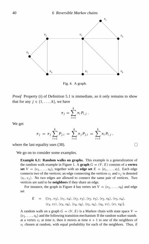
Example 6.1: Random walks on graphs.This example is a generalization ofthe random walk example in Figure 1. Agraph G = (V, E) consists of avertexsetV = {v1, . . . , vk}, together with anedge setE = {e1, . . . ,el }. Each edgeconnects two of the vertices; an edge connecting the verticesvi andv j is denoted〈vi , v j 〉. No two edges are allowed to connect the same pair of vertices. Twovertices are said to beneighbors if they share an edge.For instance, the graph in Figure 4 has vertex setV = {v1, . . . , v8} and edge
set
E = {〈v1, v3〉, 〈v1, v4〉, 〈v2, v3〉, 〈v2, v5〉, 〈v2, v6〉, 〈v3, v4〉,〈v3, v7〉, 〈v3, v8〉, 〈v4, v8〉, 〈v5, v6〉, 〈v6, v7〉, 〈v7, v8〉}.
A random walk on a graphG = (V, E) is a Markov chain with state spaceV ={v1, . . . , vk} and the following transition mechanism: If the randomwalker standsat a vertexvi at timen, then it moves at timen + 1 to one of the neighbors ofvi chosen at random, with equal probability for each of the neighbors. Thus, if

Reversible Markov chains 41
1,2
P1,1
2,1
2,2
2,3
3,2
3,3
3,4
4,3
k–1,k
k,k–1
k,k
s1
P
P
P
P
P
ss
P
P
P
P
P
s2 3 k
P
Fig. 5. Transition graph of a Markov chain of the kind discussed in Example 6.2.
we denote the number of neighbors of a vertexvi by di , then the elements of thetransition matrix are given by
Pi, j ={
1di
if vi andv j are neighbors
0 otherwise.
It turns out that random walks on graphs are reversible Markov chains, withreversible distributionπ given by
π =(d1d
,d2d
, . . . ,dkd
)(39)
whered = ∑ki=1 di . To see that (38) holds for this choice ofπ , we calculate
πi Pi, j ={
did1di
= 1d = dj
d1dj
= π j Pj,i if vi andv j are neighbors
0= π j Pj,i otherwise.
For the graph in Figure 4, (39) becomes
π =(2
24,3
24,5
24,3
24,2
24,3
24,3
24,3
24
)
so that in equilibrium,v3 is the most likely vertex for the random walker to be at,whereasv1 andv5 are the least likely ones.
Example 6.2 Let (X0, X1, . . .) be a Markov chain with state spaceS ={s1, . . . , sk} and transition matrixP, and suppose that the transition matrix hasthe properties that
(i) Pi, j > 0 whenever|i − j | = 1, and(ii) Pi, j = 0 whenever|i − j | ≥ 2.
Such a Markov chain is often called abirth-and-death process, and its transitiongraph has the form outlined in Figure 5 (with some or all of thePi,i -“loops”possibly being absent). We claim that any Markov chain of this kind is reversible.To construct a reversible distributionπ for the chain, we begin by settingπ∗
1 equalto some arbitrary strictly positive numbera. The condition (38) withi = 1 andj = 2 forces us to take
π∗2 = aP1,2
P2,1.

42 6 Reversible Markov chains
1 2
4 3
0.75
0.25
0.75
0.75
0.25
0.250.75 0.25
Fig. 6. Transition graph of the Markov chain in Example 6.3.
Applying (38) again, now withi = 2 and j = 3, we get
π∗3 = π∗
2 P2,3P3,2
= aP1,2P2,3P2,1P3,2
.
We can continue in this way, and get
π∗i = a
∏i−1l=1 Pl ,l+1∏i−1l=1 Pl+1,l
for eachi . Thenπ∗ = (π∗1 , . . . , π∗
k ) satisfies the requirements of a reversibledistribution, except possibly that the entries do not sum to 1, as is required for anyprobability distribution. But this is easily taken care of by dividing all entries bytheir sum. It is readily checked that
π = (π1, π2, . . . , πk) =(
π∗1∑k
i=1π∗i
,π∗2∑k
i=1π∗i
, . . . ,π∗k∑k
i=1π∗i
)
is a reversible distribution.
Having come this far, one might perhaps get the impression that most Markovchains are reversible. This is not really true, however, and to make up for thisfalse impression, let us also consider an example of a Markov chain which isnot reversible.
Example 6.3: A nonreversible Markov chain. Let us consider a modifiedversion of the random walk in Figure 1. Suppose that the coin tosses used bythe random walker in Figure 1 arebiased, in such a way that at each integer time,he moves one step clockwise with probability34, and one step counterclockwise
with probability 14. This yields a Markov chain with the transition graph in
Figure 6. It is clear thatπ = (14,14,14,14) is a stationary distribution for this chain
(right?). Furthermore, since the chain is irreducible, we have by Theorem 5.3 andFootnote 15 in Chapter 5 that this is the only stationary distribution. Because of

Reversible Markov chains 43
Theorem 6.1 we therefore needπ to be reversible in order for the Markov chainto be reversible. But if we, e.g., try (38) withi = 1 and j = 2, we get
π1P1,2 = 1
4· 34
= 3
16>1
16= 1
4· 14
= π2P2,1
so thatπ1P1,2 �= π2P2,1, and reversibility fails. Intuitively, the reason why thischain is not reversible is that the walker has a tendency to move clockwise. Ifwe filmed the walker and watched the movie backwards, it would look as if hepreferred to move counterclockwise, so that in other words the chain behavesdifferently in “backwards time” compared to “forwards time”.
Let us close this chapter by mentioning the existence of a simple and beautifulequivalence between reversible Markov chains on the one hand, and resistornetworks on the other. This makes electrical arguments (such as the series andparallel laws) useful for analyzing Markov chains, and conversely, probabilis-tic argument available in the study of electrical networks. Unfortunately, adiscussion of this topic would take us too far, considering the modest formatof these notes. Suggestions for further reading can be found in Chapter 14.
Problems6.1 (6) The king on the chessboard.Recall from Problem 4.3 (a) the king making
random moves on a chessboard. If you solved that problem correctly, then youknow that the corresponding Markov chain is irreducible and aperiodic. By The-orem 5.3, the chain therefore has a unique stationary distributionπ . Computeπ .Hint: the chain is reversible, and can be handled as in Example 6.1.
6.2 (8) Ehrenfest’s urn model. Fix an integerk, and imagine two urns, eachcontaining a number of balls, in such a way that the total number of balls in the twourns isk. At each integer time, we pick one ball at random (each with probability1k ) and move it to the other urn.
18 If Xn denotes the number of balls in the firsturn, then(X0, X1, . . .) forms a Markov chain with state space{0, . . . , k}.(a) Write down the transition matrix of this Markov chain.(b) Show that the Markov chain is reversible with stationary distributionπ given
by
πi = k!
i !(k− i )!2−k for i = 0, . . . , k .
(c) Show that the same distribution (known as thebinomial distribution ) alsoarises as the distribution of a binomial(k, 12) random variable, as defined inExample 1.3.
(d) Can you give an intuitive explanation of why Ehrenfest’s urn model and Ex-ample 1.3 give rise to the same distribution?
18 There are various interpretations of this model. Ehrenfest’s original intention was to modeldiffusion of molecules between the two halves of a gas container.

44 6 Reversible Markov chains
6.3 (7) Time reversal. Let (X0, X1, . . .) be a reversible Markov chain with statespaceS, transition matrixP, and reversible distributionπ . Show that if the chain isstarted with initial distributionµ(0) = π , then for anyn and anysi0, si1, . . . , sin ∈S, we have
P(X0 = si0, X1 = si1, . . . , Xn = sin) = P(X0 = sin , X1 = sin−1, . . . , Xn = si0) .
In other words, the chain is equally likely to make a tour through the statessi0, . . . sin in forwards as in backwards order.

7
Markov chain Monte Carlo
In this chapter and the next, we consider the following problem: Given a prob-ability distributionπ onS= {s1, . . . , sk}, how do we simulate a random objectwith distributionπ? To motivate the problem, we begin with an example.
Example 7.1: The hard-core model. Let G = (V, E) be a graph (recallExample 6.1 for the definition of a graph) with vertex setV = {v1, . . . , vk}and edge setE = {e1, . . . ,el }. In the so-called hard-core model onG, werandomly assign the value 0 or 1 to each of the vertices, in such a way that notwo adjacent vertices (i.e., no two vertices that share an edge) both take the value1. Assignments of 0’s and 1’s to the vertices are calledconfigurations, and canbe thought of as elements of the set{0,1}V . Configurations in which no two 1’soccupy adjacent vertices are calledfeasible. The precise way in which we picka random configuration is to take each of the feasible configurations with equalprobability. We writeµG for the resulting probability measure on{0,1}V . Hence,for ξ ∈ {0,1}V , we have
µG(ξ) ={
1ZG
if ξ is feasible
0 otherwise,(40)
whereZG is the total number of feasible configurations forG. See Figure 7 fora random configuration chosen according toµG in the case whereG is a squaregrid of size 8× 8.This model (with the graphG being a three-dimensional grid) was introduced
in statistical physics to capture some of the behavior of a gas whose particleshave nonnegligible radii and cannot overlap; here 1’s represent particles and 0’srepresent empty locations. (The model has also been used in telecommunicationsfor modelling situations where an occupied node disables all its neighboringnodes.)A very natural question is now: What is the expected number of 1’s in a random
configuration chosen according toµG? If we writen(ξ) for the number of 1’s inthe configurationξ , andX for a random configuration chosen according toµG,
45

46 7 Markov chain Monte Carlo
Fig. 7. A feasible configuration (chosen at random according to the probability measureµG), whereG is a square grid of size 8× 8. Black (resp. white) circles represent 1’s(resp. 0’s). Note that no two 1’s occupy adjacent vertices.
then this expected value is given by
E[n(X)] =∑
ξ∈{0,1}Vn(ξ)µG(ξ) = 1
ZG
∑ξ∈{0,1}V
n(ξ)I {ξ is feasible} , (41)
where ZG is the total number of feasible configurations for the graphG. Toevaluate this sum may be infeasible unless the graph is very small, since thenumber of configurations (and hence the number of terms in the sum) grows ex-ponentially in the size of the graph (for instance, we get 264 ≈ 1.8 ·1019 differentconfigurations for the moderately-sized graph in Figure 7; in physical applicationsone is usually interested in much bigger graphs). It may help somewhat thatmost of the terms take the value 0, but the number of nonzero terms growsexponentially as well. Note also that the calculation ofZG is computationallynontrivial.
When the exact expression in (41) is beyond what our computational resourcescan deal with, a good idea may be to revert to simulations. If we know how to sim-ulate a random configurationX with distributionµG, then we can do this manytimes, and estimateE[n(X)] by the average number of 1’s in our simulations.By the Law of Large Numbers (Theorem 1.2), this estimate converges to the truevalue ofE[n(X)], as the number of simulations tends to infinity, and we can formconfidence intervals etc., using standard statistical procedures.
With this example in mind, let us discuss how we can simulate a randomvariableX distributed according to a given probability distributionπ on a statespaceS. In principle it is very simple: just enumerate the elements ofS ass1, . . . , sk, and then let
X = ψ(U )
Markov chain Monte Carlo 47
whereU is a uniform [0,1] random variable, and the functionψ : [0,1] → Sis given by
ψ(x) =
s1 for x ∈ [0, π(s1))s2 for x ∈ [π(s1), π(s1) + π(s2))...
...
si for x ∈[∑i−1
j=1π(sj ),∑i
j=1π(sj ))
......
sk for x ∈[∑k−1
j=1π(sj ), 1]
(42)
as in (18). By arguing as in Chapter 3, we see thatthis givesX the desireddistributionπ . In practice, however, this approach is infeasible unless thestate spaceS is small. For the hard-core model on a square grid the size ofa chessboard or bigger, the evaluation of the functionψ in (42) becomes tootime-consuming for this method to be of any practical use.It is precisely in this kind of situation that theMarkov chain Monte Carlo
(MCMC) method is useful. The method originates in physics, where theearliest uses go back to the 1950’s. It later enjoyed huge booms in other areas,especially in image analysis in the 1980’s, and in the increasingly importantarea of statistics known asBayesian statistics19 in the 1990’s.The idea is the following: Suppose we can construct an irreducible and
aperiodic Markov chain(X0, X1, . . .), whose (unique) stationary distributionisπ . If we run the chain with arbitrary initial distribution (for instance, startingin a fixed state), then the Markov chain convergence theorem (Theorem 5.2)guarantees that the distribution of the chain at timen converges toπ , asn → ∞. Hence, if we run the chain for a sufficiently long timen, thenthe distribution ofXn will be very close toπ . Of course this is just anapproximation, but the point is that the approximation can be made arbitrarilygood by picking the running timen large.A natural objection at this stage is: How can it possibly be any easier to
construct a Markov chain with the desired property than to construct a randomvariable with distributionπ directly? To answer this, we move straight on toan example.
Example 7.2: An MCMC algorithm for the hard-core model. Let us considerthe hard-core model in Example 7.1 on a graphG = (V, E) (which for concrete-ness may be taken to be the one in Figure 7) withV = {v1, . . . , vk}. In order
19 In fact, it may be argued that the main reason that the Bayesian approach to statistics has gainedground compared to classical (frequentist) statistics is that MCMC methods have provided thecomputational tool that makes the approach feasible in practice.
48 7 Markov chain Monte Carlo
to get an MCMC algorithm for this model, we want to construct a Markov chainwhose state spaceS is the set of feasible configurations forG, i.e.,
S= {ξ ∈ {0,1}V : ξ is feasible} . (43)
In addition, we want the Markov chain to be irreducible and aperiodic, and havestationary distributionµG given by (40).AMarkov chain(X0, X1, . . .)with the desired properties can be obtained using
the following transition mechanism. At each integer timen+1, we do as follows:1. Pick a vertexv ∈ V at random (uniformly).2. Toss a fair coin.3. If the coin comes up heads, and all neighbors ofv take value 0 inXn, then let
Xn+1(v) = 1; otherwise letXn+1(v) = 0.4. For all verticesw other thanv, leave the value atw unchanged, i.e., let
Xn+1(w) = Xn(w).
It is not difficult to verify that this Markov chain is irreducible and aperiodic; seeProblem 7.1. Hence, it just remains to show thatµG is a stationary distributionfor the chain. By Theorem 6.1, it is enough to show thatµG is reversible. LettingPξ,ξ ′ denote the transition probability from stateξ to stateξ ′ (with transitionmechanism as above), we thus need to check that
µG(ξ)Pξ,ξ ′ = µG(ξ ′)Pξ ′,ξ (44)
for any two feasible configurationsξ andξ ′. Let us writed = d(ξ, ξ ′) for thenumber of vertices in whichξ andξ ′ differ, and treat the three casesd = 0,d = 1andd ≥ 2 separately. Firstly, the cased = 0 means thatξ = ξ ′, in which case therelation (44) is completely trivial. Secondly, the cased ≥ 2 is almost as trivial,because the chain never changes the values at more than one vertex at a time,making both sides of (44) equal to 0. Finally, consider the cased = 1 whereξandξ ′ differ at exactly one vertexv. Then all neighbors ofv must take the value 0in bothξ andξ ′, since otherwise one of the configurations would not be feasible.We therefore get
µG(ξ)Pξ,ξ ′ = 1
ZG
1
2k= µG(ξ ′)Pξ ′,ξ
and (44) is verified (recall thatk is the number of vertices). Hence the chain hasµG asa reversible (and therefore stationary) distribution.We can now simulate this Markov chain using the methods of Chapter 3. A
convenient choice of update functionφ is to split the unit interval [0,1] into 2ksubintervals of equal length12k , representing the choices
(v1, heads), (v1, tails), (v2, heads), . . . , (vk, tails)
in the above description of the transition mechanism. If we now run the chain fora long timen, starting with an arbitrary feasible initial configuration such as the“all 0’s” configuration, and outputXn, then we get a random configuration whosedistribution is approximatelyµG.

Markov chain Monte Carlo 49
The above is a typical MCMC algorithm in several respects. Firstly, note thatalthough it is only required that the chain has the desired distribution as astationary distribution, we found a chain with the stronger property that thedistribution is reversible. This is the case for the vast majority of knownMCMC algorithms. The reason for this is that in most nontrivial situations,the easiest way to construct a chain with a given stationary distributionπ is tomake sure that the reversibility condition (38) holds.Secondly, the algorithm in Example 7.2 is an example of a commonly used
special class of MCMC algorithms known asGibbs samplers. These areuseful to simulate probability distributionsπ on state spaces of the formSV ,whereSandV are finite sets. In other words, we have a finite setV of verticeswith a finite setSof attainable values at each vertex, andπ is the distributionof some random assignment of values inS to the vertices inV (in the hard-coremodel example, we haveS = {0,1}). The Gibbs sampler is a Markov chainwhich at each integer timen+ 1 does the following.
1. Pick a vertexv ∈ V at random (uniformly).
2. PickXn+1(v) according to the conditionalπ -distribution of the value atvgiven that all other vertices take values according toXn.
3. LetXn+1(w) = Xn(w) for all verticesw ∈ V exceptv.
It is not hard to show that this Markov chain is aperiodic, and that it hasπ as areversible (hence stationary) distribution. If in addition the chain is irreducible(which may or may not be the case depending on which elements ofSV havenonzeroπ -probability), then this Markov chain is a correct MCMC algorithmfor simulating random variables with distributionπ . We give another example:
Example 7.3: An MCMC algorithm for random q-colorings. LetG = (V, E)
be a graph, and letq ≥ 2 be an integer. Aq-coloring of the graphG is anassignment of values from{1, . . . ,q} (thought of asq different “colors”) withthe property that no two adjacent vertices have the same value (color). By arandomq-coloring forG, we mean aq-coloring chosen uniformly from the set ofpossibleq-colorings forG, and we writeρG,q for the corresponding probability
distribution20 onSV .For a vertexv ∈ V and an assignmentξ of colors to the vertices other thanv,
the conditionalρG,q-distribution of the color atv is uniform over the set of allcolors that are not attained inξ at some neighbor ofv (right?). A Gibbs sampler
20 We are here making the implicit assumption that there exists at least oneq-coloring forG. Thisis not always the case. For instance, ifq = 2 andG consists of three vertices connected ina triangle, then noq-coloring can be found. In general it is a difficult combinatorial problemto determine whetherq-colorings exist for a given choice ofG andq. The famousfour-colortheorem states that ifG is a planar graph (i.e.,G is a graph that can be drawn in the plane insuch a way that no two edges cross each other), thenq = 4 is enough.

50 7 Markov chain Monte Carlo
for randomq-colorings is therefore anSV -valued Markov chain where at eachtimen+ 1, transitions take place as follows.
1. Pick a vertexv ∈ V at random (uniformly).2. PickXn+1(v) according to the uniform distribution over the set of colors thatare not attained at any neighbor ofv.
3. Leave the color unchanged at all other vertices, i.e., letXn+1(w) = Xn(w)
for all verticesw ∈ V exceptv.
This chainis aperiodic and hasρG,q as a stationary distribution; see Problem 7.3.Whether or not the chain is irreducible depends onG andq, and it is a nontrivialproblem in general to determine this.21 In case we can show that it is irreducible,this Gibbs sampler becomes a useful MCMC algorithm.
Let us also mention that a commonly used variantof the Gibbs sampler is thefollowing. Instead of picking the vertices to update at random, we can cyclesystematically through the vertex set. For instance, ifV = {v1, . . . , vk}, wemay decide to update vertex
v1 at times 1, k+ 1,2k+ 1, . . .v2 at times 2, k+ 2,2k+ 2, . . ....
...
vi at timesi, k+ i,2k+ i, . . ....
...
vk at timesk,2k,3k, . . . .
(45)
This gives an inhomogeneous Markov chain (because there arek differentupdate rules used at different times) which is aperiodic and has the desireddistribution as a reversible distribution. Furthermore, it is irreducible if andonly if the original “random vertex” Gibbs sampler is irreducible. To provethese claims is reasonably straightforward, but requires a notationally some-what inconvenient extension of the theory in Chapters 4–6 to the case ofinhomogeneous Markov chains; we therefore omit the details. This variantof the Gibbs sampler is referredto as thesystematic sweep Gibbs sampler.Another important general procedure for designing a reversible Markov
chain for MCMC algorithms is the construction of a so-calledMetropolischain.22 Let us describe a way (not the most general possible) to con-struct a Metropolis chain for simulating a given probability distributionπ =(π1, . . . , πk) on a setS = {s1, . . . , sk}. The first step is to construct some21 Compare with the previous footnote. One thing which is not terribly hard is to show that forany given graphG, the chain is irreducible for all sufficiently largeq.
22 A more general (and widely used) class of Markov chains for MCMC simulation is that of theso-calledMetropolis–Hastings chains; see the book [GRS] mentioned in Chapter 14.

Markov chain Monte Carlo 51
graphG with vertex setS. The edge set (neighborhood structure) of this graphmay be arbitrary, except that
(i) the graph must be connected in order to assure irreducibility of the result-ing chain, and
(ii) each vertex should not be the endpoint of too many edges, since otherwisethe chain becomes computationally too heavy to simulate in practice.
As usual, we say that two statessi andsj are neighbors if the graph containsan edge〈si , sj 〉 linking them. We also writedi for the number of neighborsof statesi . The Metropolis chain corresponding to a given choice ofG hastransition matrix
Pi, j =
1dimin
{π j diπi dj
,1}
if si andsj are neighbors
0 if si �= sj are not neighbors1−
∑l
sl∼si
1dimin
{πl diπi dl
,1}
if i = j ,(46)
where the sum is over all statessl that are neighbors ofsi . This transitionmatrix corresponds to the following transition mechanism: Suppose thatXn =si . First pick a statesj according to uniform distribution on the set of neighborsof si (so that each neighbor is chosen with probability1di ). Then set
Xn+1 =sj with probability min
{π j diπi dj
,1}
si with probability 1−min{π j di
πi dj,1
}.
To show that this Markov chain hasπ as its stationary distribution, it is enoughto verify that the reversibility condition
πi Pi, j = π j Pj,i (47)
holds for alli and j . We proceed as in Example 7.2, by first noting that (47)is trivial for i = j . For the case wherei �= j andsi andsj are not neighbors,(47) holds because both sides are 0. Finally, we split the case wheresi andsj are neighbors into two subcases according to whether or not
π j diπi dj
≥ 1. Ifπ j diπi dj
≥ 1, then
πi Pi, j = πi1di
π j Pj,i = π j1dj
πi djπ j di
= πidi
52 7 Markov chain Monte Carlo
so that (47) holds. Similarly, ifπ j diπi dj
< 1, then
πi Pi, j = πi1di
π j diπi dj
= π jdj
π j Pj,i = π j1dj
and again (47) holds. Soπ is a reversible (hence stationary) distribution forthe Metropolis chain, which therefore can beused for MCMC simulation ofπ .
Problems7.1 (5) Show that the Markov chain used for MCMC simulation of the hard-core
model in Example 7.2 is
(a) irreducible,23 and(b) aperiodic.24
7.2 (8*) Write a computer program, using the algorithm in Example 7.2, for simulat-ing the hard-core model on a generalk × k square grid. Then do some simulationexperiments.25
7.3 (7) Show, by arguing as in Example 7.2 and Problem 7.1 (b), that the Gibbssampler for randomq-colorings in Example 7.3
(a) hasρG,q as a stationary distribution, and(b) is aperiodic.
7.4 (6) A generalized hard-core model.A natural generalization of the hard-coremodel is to allow for different “packing intensities” of 1’s in the graph. This isdone by introducing a parameterλ > 0, and changing the probability measureµG defined in (40) into a probability measureµG,λ in which each configurationξ ∈ {0,1}V gets probability
µG,λ(ξ) ={
λn(ξ)
ZG,λif ξ is feasible
0 otherwise,(48)
wheren(ξ) is the number of 1’s inξ , andZG,λ = ∑ξ∈{0,1}V λn(ξ)I {ξ is feasible}
is a normalizing constant. As follows from a direct calculation,this means that for
23 Hint: We need to show that for any two feasible configurationsξ andξ ′, the chain can go fromξ to ξ ′ in a finite number of steps. The easiest way to show this is to demonstrate that it cango fromξ to the “all 0’s” configuration in a finite number of steps, and then from the “all 0’s”configuration toξ ′ in a finite number of steps.
24 Hint: To show that the period of a stateξ is 1, it is enough to show that the Markov chain cango fromξ to ξ in one step (see also Problem 4.2).
25 When you have managed to do this for, say, a 10× 10 square lattice, consider the following:Think back to Example 2.3 (the Internet as a Markov chain). Did that example seem to have aridiculously huge state space? Well, you have just simulated a Markov chain whose state spaceis even bigger! It is not hard to show that the state spaceSas defined in (43) contains at least
2k2/2 = 250 ≈ 1.1 ·1015 elements – much larger than the number of web pages on the Internet
today.
Markov chain Monte Carlo 53
any vertexv ∈ V , the conditional probability thatv takes the value 1, given thevalues at all other vertices, equals{
λλ+1 if all neighbors ofv take value 0
0 otherwise.
The model’s “desire” to put a 1 atv therefore increases gradually asλ increasesfrom 0 to ∞. The caseλ = 1 reduces to the standard hard-core model inExample 7.1.Construct an MCMC algorithm for this generalized hard-core model.

8
Fast convergence of MCMC algorithms
Although the MCMC approach to simulation, described in the previous chap-ter, is highly useful, let us note two drawbacks of the method:
(A) The main theoretical basis for the MCMC method is Theorem 5.2, whichguarantees that the distributionµ(n) at timen of an irreducible and ape-riodic Markov chain started in a fixed state converges to the stationarydistributionπ asn → ∞. But this does not imply thatµ(n) ever becomesequalto π , only that it comes very close. As a matter of fact, in the vastmajority of examples, we haveµ(n) �= π for all n (see, e.g., Problem 2.3).Hence, no matter how largen is taken to be in the MCMC algorithm, therewill still be some discrepancy between the distribution of the output andthe desired distributionπ .
(B) In order to make the error due to (A) small, we need to figure out how largen needs to be taken in order to make sure that the discrepancy betweenµ(n) and π (measured in the total variation distance dTV(µ(n), π)) issmaller than some givenε > 0. In many situations, it has turned outto be very difficult to obtain upper bounds on how largen needs to betaken, that are small enough to be of any practical use.26
Problem (A) above is in itself not a particularly serious obstacle. In mostsituations, we can tolerate a small error in the distribution of the output, as longas we have an idea about how small it is. It is only in combination with (B)that it becomes really bothersome. Due to difficulties in determining the rate of
26 In general, it is possible to extract an explicit upper bound (depending onε and on the chain)by a careful analysis of the proof of Theorem 5.2. However, this often leads to bounds ofastronomical magnitude, such as “dTV(µ(n), π) < 0.01 whenevern ≥ 10100”. This is ofcourse totally useless, because the simulation of 10100 steps of a Markov chain is unlikely toterminate during our lifetimes. In such situations, one can often suspect that the convergence ismuch faster (so that perhapsn = 105 would suffice), but to actually prove this often turns outto be prohibitively difficult.
54

Fast convergence of MCMC algorithms 55
convergence to stationarity in Markov chains, much of today’s MCMC practicehas the following character: A Markov chain (X0, X1, . . .) whose distributionµ(n) converges to the desired distributionπ , as the running timen tends to∞,is constructed. The chain is then run for a fairly long timen (say, 104 or 105),andXn is output, in the hope that the chain has come close to equilibrium bythen. But this is often just a matter of faith, or perhaps some vague handwavingarguments.This situation is clearly unsatisfactory, and a substantial amount of effort
has in recent years been put into attempts at rectifying it. In this chapter and inChapters 10–12, we shall take a look at two different approaches. The one weconsider in this chapter is to try to overcome the more serious problem (B) byestablishing useful bounds for convergence rates of Markov chains. In general,this remains a difficult open problem, but in a number of specific situations,very good results have been obtained.To illustrate the type of convergence rate results that can be obtained, and
one of themain proof techniques, wewill in this chapter focus on one particularexample where the MCMC chain has been successfully analyzed, namely therandomq-colorings in Example 7.3.A variety of different(but sometimes related) techniques for proving fast
convergence to equilibrium of Markov chains have been developed, includingeigenvalue bounds, path and flow arguments, various comparisons betweendifferent chains, and the concept of strong stationary duality; see Chapter 14for some references concerning these techniques. Another important tech-nique, that we touched upon already in Chapter 5, is the use of couplings,and that is the approach we shall take here.Let us consider theq-coloring example. Fix a graphG = (V, E) and an
integerq, and recall thatρG,q is the probability distribution on{1, . . . ,q}Vwhich is uniform over allξ ∈ {1, . . . ,q}V that are validq-colorings, i.e.,over all assignments of colors 1, . . . ,q to the vertices ofG with the propertythat no two vertices sharing an edge have the same color. We consider theGibbs sampler described in Example 7.3, with the modification that the vertexto be updated is chosen as in the systematic sweep Gibbs sampler defined in(45). This means that instead of picking a vertex at random uniformly fromV = {v1, . . . , vk}, we scan systematically through the vertex set by updatingvertexv1 at time 1,v2 at time 2,. . . , vk at timek, v1 again at timek + 1, andso on as in (45).It is natural to phrase the question about convergence rates for this MCMC
algorithm (or others) as follows: Givenε > 0 (such as for instanceε = 0.01),how many iterationsn of the algorithm do we need in order to make the totalvariation distance dTV(µ(n), ρG,q) less thanε? Hereµ(n) is the distribution ofthe chain aftern iterations.

56 8 Fast convergence of MCMC algorithms
Theorem 8.1Let G = (V, E) be a graph. Let k be the number of verticesin G, and suppose that any vertexv ∈ V has at most d neighbors. Supposefurthermore that q> 2d2. Then, for any fixedε > 0, the number of iterationsneeded for the systematic sweep Gibbs sampler described above (starting fromany fixed q-coloringξ ) to come within total variation distanceε of the targetdistributionρG,q is at most
k
log(k) + log(ε−1) − log(d)
log(
q2d2
) + 1
. (49)
Before going to the proof of this result, some comments are in order:
1. The most important aspect of the bound in (49) is that it is bounded by
Ck(log(k) + log(ε−1))
for some constantC < ∞ that does not depend onk or onε. This meansthat the number of iterations needed to come within total variation distanceε from the target distributionρG,q does not grow terribly quickly ask → ∞or asε → 0. It is easy to see thatanyalgorithm for generating randomq-colorings must have a running time that grows at least linearly ink (becauseit takes about timek even toprint the result). The extra factor log(k) thatwe get here is not a particularly serious slowdown.
2. Our boundq > 2d2 for when we get fast convergence is a fairly crudeestimate. In fact, Jerrum [J] showed, by means of a refined version of theproof below, that a convergence rate of the same order of magnitude as inTheorem 8.1 takes place as soon asq > 2d, and it is quite likely that thisbound can be improved even further.
3. If G is part of the square lattice (such as, for example, the graph in Figure 7),thend = 4, so that Theorem 8.1 gives fast convergence of the MCMCalgorithm forq ≥ 33. Jerrum’s better bound gives fast convergence forq ≥ 9.
4. It may seem odd that we obtain fast convergence for largeq only, as onemight intuitively think that it would be more difficult to simulate the largerq gets, due to the fact that the number ofq-colorings onG is increasing inq. This is, however, misleading, and the correct intuition to have is insteadthe following. The largerq gets, the less dependent does the coloring ofa vertexv become on its neighbors. Ifq is very large, we might pick thecolor atv uniformly at random, and have very little risk that this color isalready taken by one of its neighbors. Hence, the difference betweenρG,q
and uniform distribution overall elements of{1, . . . ,q}V becomes very

Fast convergence of MCMC algorithms 57
small in the limit asq → ∞, and the latter distribution is of course easy tosimulate: just assign i.i.d. colors (uniformly from{1, . . . ,q}) to the vertices.
Enough chat for now – it is time to do the five-page proof of the convergencerate result!
Proof of Theorem 8.1As in the proof of Theorem 5.2, we will use a couplingargument: We shall run two{1, . . . ,q}V -valued Markov chains(X0, X1, . . .)and(X′
0, X′1, . . .) simultaneously. They will have the same transition matrices
(namely, the ones given by the systematic sweep Gibbs sampler for randomq-colorings ofG, as described above). The difference will be that the firstchain is started in the fixed stateX0 = ξ , whereas the second is started in arandom stateX′
0 chosen according to the stationary distributionρG,q. ThenX′n has distributionρG,q for all n, by the definition of stationarity. Also write
µ(n) for the distribution of the first chain(X0, X1, . . .) at timen; this is thechain that we are primarily interested in. We want to bound the total variationdistance dTV(µ(n), ρG,q) betweenµ(n) and the stationary distribution, and weshall see that dTV(µ(n), ρG,q) is close to 0 ifP(Xn = X′
n) is close to 1.Recall from Example 7.3 that whenever a vertexv is chosen to be updated,
we should pick a new color forv according to the uniform distribution on theset of colors that are not attained by any neighbor ofv. One way to implementthis concretely is to pick a random permutation
R= (R1, . . . , Rq)
of the set{1, . . . ,q}, chosen uniformly from theq! different possible permu-tations (this is fairly easy; see Problem 8.1) and then letv get the first color ofthe permutation that is not attained by any neighbor ofv.Of course we need to pick a new (and independent) permutation at each
update of a chain. However, nothing prevents us from usingthe same permu-tations for the chain(X′
0, X′1, . . .) as for(X0, X1, . . .), and this is indeed what
we shall do. LetR0, R1, . . . be an i.i.d. sequence of random permutations, eachof them uniformly distributed on the set of permutations of{1, . . . ,q}. At eachtimen, the updates of the two chains use the permutation
Rn = (R1n, . . . , Rqn) ,
and the vertexv to be updated is assigned the new value
Xn+1(v) = Rin
where
i = min{ j : Xn(w) �= Rjn for all neighborsw of v}

58 8 Fast convergence of MCMC algorithms
in the first chain. In the second chain, we similarly set
X′n+1(v) = Ri
′n
where
i ′ = min{ j ′ : X′n(w) �= Rj
′n for all neighborsw of v} .
This defines our coupling of(X0, X1, . . .) and(X′0, X
′1, . . .). What we hope
for is to haveXT = X′T at some (random, but not too large) timeT , in which
case we will also haveXn = X′n for all n ≥ T (because the coupling is defined
in such a way that once the two chains coincide, they stay together forever). Inorder to estimate the probability that the configurationsXn andX′
n agree, letus first consider the probability that they agreeat a particular vertex, i.e., thatXn(v) = X′
n(v) for a given vertexv.Consider the update of the two chains at a vertexv at timen, where we
taken ≤ k, so that in other words we are in the first sweep of the Gibbssampler through the vertex set. We call the updatesuccessfulif it results inhavingXn+1(v) = X′
n+1(v); otherwise we say that the update isfailed. Theprobability of a successful update depends on the number of colors that areattained in the neighborhood ofv in both configurationsXn andX′
n, and onthe number of colors that are attained in each of them. Define
B2 = the number of colorsr ∈ {1, . . . ,q} that are attained in theneighborhood ofv in both Xn andX′
n,
B1 = the number of colorsr ∈ {1, . . . ,q} that are attained in theneighborhood ofv in exactly oneof Xn andX′
n,
and
B0 = the number of colorsr ∈ {1, . . . ,q} that are attained in theneighborhood ofv in neitherof Xn andX′
n,
and note thatB0 + B1 + B2 = q. Note also that if the first colorR1n in thepermutationRn is among theB2 colors attained in the neighborhood ofv inboth configurations, then the Gibbs samplers just discardR1n and look atR
2n
instead, and so on. Therefore, the update is successful if and only if the firstcolor in Rn that is attained in the neighborhood ofv in neitherof Xn andX′n appears earlier in the permutation than the first color that is attained in
the neighborhood ofv in exactly oneof Xn andX′n. This event (of having a
successful update) therefore has probability
B0B0 + B1

Fast convergence of MCMC algorithms 59
conditional onB0, B1 andB2. In other words, we have27
P(failed update) = B1B0 + B1
. (50)
We go on to estimate the right-hand side in (50). Clearly, 0≤ B2 ≤ d.Furthermore,
B1 ≤ 2d − 2B2 , (51)
because counting the neighbors in both configurations, there are in all at most2d of them, and each color contributing toB2 uses up two of them. We get
P(failed update) = B1B0 + B1
= B1q − B2
≤ 2d − 2B2q − B2
≤ 2d − B2q − B2
= 2d(1− B2
2d
)q(1− B2
q
) ≤ 2d
q(52)
where the first inequality is just (51), while the final inequality is due to theassumptionq > 2d2, which impliesq > 2d, which in turn implies
(1− B2
q
) ≥(1− B2
2d
).
Hence, we have, afterk steps of the Markov chains (i.e., after the first sweepof the Gibbs samplers through the vertex set), that, for each vertexv,
P(Xk(v) �= X′k(v)) ≤ 2d
q. (53)
Now consider updates during the second sweep of the Gibbs sampler, i.e.,between timesk and 2k. For an update at timen during the second sweep tofail, the configurationsXn andX′
n need to differ in at least one neighbor ofv. Each neighborw hasXn(w) �= X′
n(w) with probability at most2dq (due to(53)), and summing over the at mostd neighbors, we get that
P(discrepancy) ≤ 2d2
q(54)
where “discrepancy” is short for the event that there exists a neighborw
of v with Xn(w) �= X′n(w). Given the event in (54), we have, by re-
peating the arguments in (50) and (52), that the conditional probability
27 Our notation here is a bit sloppy, since it is really a conditional probability we are dealing with,because we are conditioning onB0, B1 andB2.

60 8 Fast convergence of MCMC algorithms
P(failed update|discrepancy) of a failed update is bounded by2dq . Hence,P(failed update) = P(discrepancy)P(failed update|discrepancy)
≤ 4d3
q2= 2d
q
(2d2
q
).
Hence, after 2k steps of the Markov chains, each vertexv ∈ V has differentcolorsin the two chains with probability at most
P(X2k(v) �= X′2k(v)) ≤ 2d
q
(2d2
q
).
By arguing in the same way for the third sweep as for the second sweep, weget that
P(X3k(v) �= X′3k(v)) ≤ 2d
q
(2d2
q
)2,
and continuing in the obvious way, we get form= 4,5, . . . that
P(Xmk(v) �= X′mk(v)) ≤ 2d
q
(2d2
q
)m−1. (55)
After this analysis of the probability thatXmk and X′mk differ at a given
vertex, we next want to estimate the probabilityP(Xmk �= X′mk) that the first
chain fails to haveexactly the same configurationas the second chain, at timemk. Since the eventXmk �= X′
mk implies thatXmk(v) �= X′mk(v) for at least
one vertexv ∈ V , we have
P(Xmk �= X′mk) ≤
∑v∈V
P(Xmk(v) �= X′mk(v))
≤ k2d
q
(2d2
q
)m−1(56)
= k
d
(2d2
q
)m(57)
where the inequality in (56) is due to (55) and the assumption that the graphhask vertices.Now let A ⊆ {1, . . . ,q}V be any subset of{1, . . . ,q}V . By (33) and
Problem 5.1, we have that
dTV(µ(mk), ρG,q) = maxA⊆{1,...,q}V
∣∣∣µ(mk)(A) − ρG,q(A)
∣∣∣= max
A⊆{1,...,q}V∣∣P(Xmk ∈ A) − P(X′
mk ∈ A)∣∣ . (58)

Fast convergence of MCMC algorithms 61
For any suchA, we have
P(Xmk ∈ A) − P(X′mk ∈ A)
= P(Xmk ∈ A, X′mk ∈ A) + P(Xmk ∈ A, X′
mk �∈ A)
− (P(X′
mk ∈ A, Xmk ∈ A) + P(X′mk ∈ A, Xmk �∈ A)
)= P(Xmk ∈ A, X′
mk �∈ A) − P(X′mk ∈ A, Xmk �∈ A)
≤ P(Xmk ∈ A, X′mk �∈ A)
≤ P(Xmk �= X′mk)
≤ k
d
(2d2
q
)m(59)
where the last inequality uses (57). Similarly, we get
P(X′mk ∈ A) − P(Xmk ∈ A) ≤ k
d
(2d2
q
)m. (60)
Combining (59) and (60), we obtain
∣∣P(Xmk ∈ A) − P(X′mk ∈ A)
∣∣ ≤ k
d
(2d2
q
)m. (61)
By taking the maximum over allA ⊆ {1, . . . ,q}V , and inserting into (58), weget that
dTV(µ(mk), ρG,q) ≤ k
d
(2d2
q
)m, (62)
which tends to 0 asm→ ∞. Having established this bound, our next and finalissue is:
How large doesm need to be taken in order to make the right-hand sideof (62) less thanε?
By setting
k
d
(2d2
q
)m= ε
and solving form, we find that
m= log(k) + log(ε−1) − log(d)
log(
q2d2
)so that running the Gibbs sampler long enough to get at least this many scans

62 8 Fast convergence of MCMC algorithms
through the vertex set gives dTV(µ(mk), ρG,q) ≤ ε. To go from the number ofscansm to the number of stepsn of the Markov chain, we have to multiply byk, giving that
n = k(log(k) + log(ε−1) − log(d))
log( q2d2
) (63)
should be enough. However, by takingn as in (63), we do not necessarily getan integer value form = n
k , so to be on the safe side we should taken to be atleast the smallest number which is greater than the right-hand side of (63) andwhich makesnk an integer. This means increasingn by at mostk compared to(63), so thatourfinal answer isthat taking
n = k
(log(k) + log(ε−1) − log(d)
log( q2d2
) + 1
)
suffices, and Theorem 8.1 is (at last!) established.
Problems8.1 (4) Describe a simple and efficient way to generate a random (uniform distribu-
tion) permutation of the set{1, . . . ,q}.8.2 (6) Bounding total variation distance using coupling. Let π1 and π2 be
probability distributions on some finite setS. Suppose that we can construct tworandom variablesY1 andY2 such that
(i) Y1 has distributionπ1,
(ii) Y2 has distributionπ2, and
(iii) P(Y1 �= Y2) ≤ ε,
for some givenε ∈ [0,1]. Show that the total variation distance dTV(π1, π2) is atmostε. Hint: argue as in equations (59), (60) and (61) in the proof of Theorem 8.1.
8.3 (8) Explain where and why the assumption thatq > 2d2 is needed in the proofof Theorem 8.1.
8.4 (10) Fast convergence for the random site Gibbs sampler.Consider (insteadof the systematic scan Gibbs sampler) the random site Gibbs sampler for randomq-colorings, as in Example 7.3. Suppose that the graphG = (V, E) hask vertices,and each vertex has at mostd neighbors. Also suppose thatq > 2d2.
(a) Show that for any givenv ∈ V , the probability thatv is chosen to be updatedat some step during the firstk iterations of the Markov chain is at least 1−e−1.(Heree≈ 2.7183 is, of course, the base for the natural logarithm.)
(b) Suppose that we run two copies of this Gibbs sampler, one starting in a fixedconfiguration, and one in equilibrium, similarly as in the proof of Theorem 8.1.Show that the coupling can be carried out in such a way that for anyv ∈ V andanym, the probability that the two chains have different colors at the vertexv
Fast convergence of MCMC algorithms 63
at timemk is at most(e−1+ (1− e−1)2d
q
)(e−1+ (1− e−1)2d
2
q
)m−1.
(c) Use the result in (b) to prove an analogue of Theorem 8.1 for the random siteGibbs sampler.

9
Approximate counting
Combinatorics is the branch of mathematics whichdeals withfinite objectsor sets, and the ways in which these can be combined. Basic objects thatoften arise in combinatorics are, e.g., graphs and permutations. Much ofcombinatorics deals with the following sort of problem:
Given some setS, what is the number of elements ofS?
Let us give afew examples of suchcounting problems; the reader willprobably be able to think of several interesting variations of these.
Example 9.1What is the number of permutationsr = (r 1, . . . , r q) of the set{1, . . . ,q} with the property that no two numbers that differ by exactly 1 areadjacent in the permutation?
Example 9.2Imagine a chessboard, and a set of 32 domino tiles, such that onetile is exactly large enough to cover two adjacent squares of the chessboard. Inhow many different ways can the 32 tiles be arranged so as to cover the entirechessboard?
Example 9.3Given a graphG = (V, E), in how many ways can we pick a subsetW of the vertex setV , with the property that no two vertices inW are adjacentin G? In other words, how many different feasible configurations exist for thehard-core model (see Example 7.1) onG?
Example 9.4Given an integerq and a graphG = (V, E), how many differentq-colorings (Example 7.3) are there forG?
In this chapter, we are interested in algorithms for solving counting problems.For the purpose of illustrating some general techniques, we shall focus on theone in Example 9.4: the number ofq-colorings of a graph. In particular, weshall see how (perhaps surprisingly!) the MCMC technique turns out to beuseful in the context of counting problems. The same general approach has
64

Approximate counting 65
proved to be successful in a host of other counting problems, including count-ing of feasible hard-core configurations and of domino tilings, and estimationof the normalizing constantZG,β in the so-called Ising model (which will bediscussed in Chapter 11); see Sinclair [Si] for an overview.The following algorithm springs immediately to mind as a solution to the
problem of countingq-colorings.
Example 9.5: A naive algorithm for counting q-colorings. If there were norestriction on the colorings, i.e., if all configurations in{1, . . . ,q}V were allowed,then the counting problem would be trivial: there areqk of them, wherek is thenumber of vertices in the graph. Moreover, it is trivial to make a list of all suchconfigurations, for instance in some lexicographic order. Given a configurationξ ∈ {1, . . . ,q}V , the problem of determining whetherξ is a properq-coloring ofG is yet another triviality.28 Hence, the following algorithm will work:
Go through all configurations in{1, . . . ,q}V in lexicographic order, checkfor each of them whether it is aq-coloring ofG, and count the number oftimes the answer was “yes”.
This algorithm will certainly give the right answer. However, whenk is large, itwill take a very long time to run the algorithm, since it has to work itself throughthe list of all qk configurations. For instance, whenq = 5 andk = 50, thereare 550 ≈ 1034 configurations to go through, which is impossible in practice.Therefore, this algorithm will only be useful for rather small graphs.
The feature which makes the algorithm in Example 9.5 unattractive is that therunning time grows exponentially in the sizek of the graph. The challenge inthis type of situation is therefore to find faster algorithms. In particular, one isinterested inpolynomial time algorithms, i.e., algorithms with the propertythat there exists a polynomialp(k) in the sizek of the problem,29 such that therunning time is bounded byp(k) for any k and any instance of the problemof sizek. This is the same (see Problem 9.1) as asking for algorithms with arunning time bounded byCkα for some constantsC andα.A polynomial time algorithm which solves a counting problem is called a
polynomial time counting schemefor the problem. Sometimes, however,such an algorithm is not available, and we have to settle for something less,namely toapproximate(rather than calculate exactly) the number of elements
28 We just need to check, for each edgee∈ E, that the endvertices ofehave different colors.29 Here we measure the size of the problem in the number of vertices in the graph. This is usuallythe most natural choice for problems involving graphs, although sometimes there is reason takethe number of edges instead. In Example 9.1, it is natural to takeq as the size of the problem,whereas in generalizations of Example 9.2 to “chessboards” of arbitrary size, the size of theproblem may be measured in the number of squares of the chessboard (or in the number ofdomino tiles). Common to all these measures of size is that the number of elements in the setto be counted grows (at least) exponentially in the size of the problem, making algorithms likethe one in Example 9.5 infeasible.

66 9 Approximate counting
of the set. Suppose that we have an algorithm which, in addition to the instanceof the counting problem, also takes a numberε > 0 as input. Supposefurthermore that the algorithm has the properties that
(i) it always outputs an answer between(1− ε)N and(1+ ε)N, whereN isthe true answer to the counting problem, and
(ii) for any ε > 0, there exists a polynomialpε(k) in the sizek of theproblem,30 such that for any instance of sizek, the algorithm terminatesin at mostpε(k) steps.
We call such an algorithm apolynomial time approximation scheme. Givena prespecifiedallowed relative errorε, the algorithm runs in polynomial timein the size of the problem, and produces an answer which is within a multi-plicative errorε of the true answer.Sometimes, however, even this is too much to ask, and we have to be
content with an algorithm which produces an almost correct answer most ofthe time, but which may produce a (vastly) incorrect answer with some positiveprobability. More precisely, suppose that we have an algorithm which takesε > 0 and the instance of the counting problem as input, and has the propertiesthat
(i) with probability at least23, it outputs an answer between(1 − ε)N and(1+ ε)N, whereN is the true answer to the counting problem, and
(ii) for any ε > 0, there exists a polynomialpε(k) in the sizek of the problem,such that for any instance of sizek, the algorithm terminates in at mostpε(k) steps.
Such an algorithm is called arandomized polynomial time approximationscheme, and it is to the construction of such a scheme (for theq-coloringcounting problem) that this chapter is devoted.One may (and should!) ask at this stage what is so special about the number
23. The answer is that it is, in fact, not special at all, and that it could be replacedby any number strictly between12 and 1. For instance, for anyδ > 0, if wehave a randomized polynomial time approximation scheme (with the abovedefinition), then it is not difficult to build further upon it to obtain a randomizedpolynomial time approximation scheme with the additional property that itoutputs an answer within a multiplicative errorε of the true answer, withprobability at least 1− δ. We can thus get an answer within relative errorat mostε of the true answer, with probability as close to 1 as we may wish.This property will be proved Problem 9.3 below.
30 We allow pε(k) to depend onε in arbitrary fashion. Sometimes (although we shall not go intothis subtlety) there is reason to be restrictive about how fastpε(k) may grow asε → 0.

Approximate counting 67
Here is our main result concerning randomized polynomial time approxima-tion schemes for randomq-colorings.
Theorem 9.1Fix integers q and d≥ 2 such that q> 2d2, and consider theproblem of counting q-colorings for graphs in which each vertex has at most dneighbors. There exists a randomized polynomial time approximation schemefor this problem.
Before going on with the proof of this result, some remarks are worth making:
1. Of course, an existence result (i.e., a statement of the form “there exists analgorithm such that. . .”) of this kind is rather useless without an explicitdescription of the algorithm. Such a description, will, however, appearbelow as part of the proof.
2. The requirement thatq > 2d2 comes from Theorem 8.1, which will beused in the proof of Theorem 9.1. If we instead use Jerrum’s better resultmentioned in Remark 2 after Theorem 8.1, then we obtain the same resultas in Theorem 9.1 wheneverq > 2d.
3. The restriction tod ≥ 2 is not a particularly severe one, since graphs withd = 1 consist just of
(i) isolated vertices (having no neighbors), and
(ii) pairs of vertices linked to each other by an edge but with no edgeleading anywhere else,
and the number ofq-colorings of such graphs can be calculated directly(see Problem 9.2).
Another thing which it is instructive to do before the proof of Theorem 9.1 is tohave a look at the following simple-minded attempt at a randomized algorithm,and to figure out why it does not work well in practice.
Example 9.6: Another naive algorithm for counting q-colorings. AssumethatG = (V, E) is connected withk vertices, and writeZG,q for the numberof q-colorings ofG. Suppose that we assign each vertex independently a colorfrom {1, . . . ,q} chosen according to the uniform distribution, without regard towhether or not adjacent vertices have the same color. Then each configurationξ ∈ {1, . . . ,q}V arises with the same probability1
qk. Out of theseqk possible
configurations, there areZG,q that areq-colorings, whence the probability thatthis procedure yields aq-coloring is
ZG,q
qk. (64)

68 9 Approximate counting
Let us now repeat this experimentn times, and writeYn for the number of timesthat we gotq-colorings. We clearly have
E[Yn] = nZG,q
qk
so that
E
[qkYnn
]= ZG,q
which suggests thatqkYnn might be a good estimator ofZG,q. Indeed, the Law of
Large Numbers (Theorem 1.2) may be applied to show, for anyε > 0, that qkYnn
is between(1− ε)ZG,q and(1+ ε)ZG,q with a probability which tends to 1 asn → ∞.But how large doesn need to be? Clearly,q
kYnn is a very bad estimate as long
asYn = 0, so we certainly need to pickn sufficiently large to makeYn > 0 with areasonably high probability. Unfortunately, this means thatn has to be takenverylarge, as the following argument shows. In each simulation, we get aq-coloring
with probability at most(q−1q
)k−1; this is Problem 9.4. Hence,
P(Yn > 0) = P(at least one of the firstn simulations yields aq-coloring)
≤n∑i=1
P(the i th simulation yields aq-coloring)
≤ n
(q − 1
q
)k−1.
To make this probability reasonably large, say greater than12, we need to take
n ≥ 12
(qq−1
)k−1. This quantity grows exponentially ink, making the algorithm
useless for large graphs.
Let us pause for a moment and think about precisely what it is that makes thealgorithm in Example 9.6 so creepingly slow. The reason is a combinationof two facts: First, the probability in (64) that we are trying to estimate isextremely small: exponentially small in the number of verticesk. Second,to estimate a very small probability by means of simulation requires a verylarge number of simulations. In the algorithm that we are about to present aspart of the proof of Theorem 9.1, one of the key ideas is to find other relevantprobabilities to estimate, which have a more reasonable order of magnitude.Let us now turn to the proof.
First part of the proof of Theorem 9.1: a general description of the algo-rithm Suppose that the graphG = (V, E) hask vertices andk edges; bythe assumption of the theorem we have thatk ≤ dk. Enumerate the edge

Approximate counting 69
set E as {e1, . . . ,ek}, and define the subgraphsG0,G1, . . . ,Gk as follows.Let G0 = (V, ∅) be the graph with vertex setV and no edges, and forj = 1, . . . , k, let
Gj = (V, {e1, . . . ,ej }) .
In other words,Gj is the graph obtained fromG by deleting the edgesej+1, . . . ,ek.Next, let, for j = 0, . . . , k, the number ofq-colorings for the graphGj be
denoted byZ j . SinceGk = G, we have that the number we wish to compute(or approximate) isZk. This number can be rewritten as
Zk = ZkZk−1
× Zk−1Zk−2
× · · · × Z2Z1
× Z1Z0
× Z0 . (65)
If we can estimate each factor in the telescoped product in (65) to withinsufficient accuracy, then we can multiply these estimates to get a reasonablyaccurate estimate ofZk.Note first that the last factorZ0 is trivial to calculate: sinceG0 has no edges,
any assignmentof colors from{1, . . . ,q} to the verticesis a validq-coloring,and sinceG0 hask vertices, we have
Z0 = qk .
Consider next one of the other factorsZ jZ j−1 in (65). Write xj and yj for
the endvertices of the edgeej which is inGj but not inGj−1. By definition,Z j is the number ofq-colorings of the graphGj . But theq-colorings ofGj
are exactly those configurationsξ ∈ {1, . . . ,q}V that areq-colorings ofGj−1and that in addition satisfyξ(xj ) �= ξ(yj ). Hence the ratio
Z jZ j−1 is exactly the
proportion ofq-coloringsξ of Gj that satisfyξ(xj ) �= ξ(yj ). This means that
Z jZ j−1
= ρGj−1,q(X(xj ) �= X(yj )) , (66)
i.e.,Z jZ j−1 equals the probability that a random coloringX of Gj−1, chosen
according to the uniform distributionρGj−1,q, satisfiesX(xj ) �= X(yj ).The key point now is that the probabilityρGj ,q(X(xj ) �= X(yj )) in (66)
can be estimated using the simulation algorithm forρGj−1,q considered inTheorem 8.1. Namely, if we simulate a randomq-coloring X ∈ {1, . . . ,q}Vfor Gj−1 several times(using sufficiently manysteps in the Gibbs sampler ofChapter 8), then the proportion of the simulations that result in a configurationwith different colors atxj and yj is very likely to be close31 to the desired
31 This closeness is due to the Law of Large Numbers (Theorem 1.2).

70 9 Approximate counting
expression in (66). We use this procedure to estimate each factor in thetelescoped product in (65), and then multiply these to get a good estimate oftheZk.
The second part of the proof of Theorem 9.1 consists of figuring out howmany simulations we need to do for estimating each factor
Z jZ j−1 , and how
many steps of the Gibbs sampler we need to run in each simulation. For that,we first need three little lemmas:
Lemma 9.1Fix ε ∈ [0,1], let k be a positive integer, and let a1, . . . ,ak andb1, . . . ,bk be positive numbers satisfying(
1− ε
2k
)≤ ajbj
≤(1+ ε
2k
)
for j = 1, . . . , k. Define the products a= ∏kj=1 aj and b= ∏k
j=1 bj . Wethen have
1− ε ≤ a
b≤ 1+ ε . (67)
Proof To prove the first inequality in (67), note that(1− ε2k )
2 ≥ 1− 2ε2k , that
(1− ε2k )
3 ≥ (1− ε2k )(1− 2ε
2k ) ≥ 1− 3ε2k , and so on, so that(
1− ε
2k
)k ≥ 1− kε
2k.
Hence,
a
b=
k∏j=1
ajbj
≥k∏j=1
(1− ε
2k
)=
(1− ε
2k
)k
≥ 1− kε
2k= 1− ε
2≥ 1− ε .
For the second inequality, we note thatex/2 ≤ 1+ x for all x ∈ [0,1] (plot thefunctions to see this!), so that
a
b=
k∏j=1
ajbj
≤k∏j=1
(1+ ε
2k
)≤
k∏j=1exp
( ε
2k
)
= exp(ε
2
)≤ 1+ ε .
Lemma 9.2Fix d ≥ 2 and q > 2d2. Let G = (V, E) be a graph in whichno vertex has more than d neighbors, and pick a random q-coloring X for G

Approximate counting 71
according to the uniform distributionρG,q. Then, for any two distinct verticesx, y ∈ V , the probability that X(x) �= X(y) satisfies
ρG,q(X(x) �= X(y)) ≥ 1
2. (68)
Proof Note first that whenx and y are neighbors inG, then (68) is trivial,since its left-hand side equals 1. We go on to consider the case wherex andyare not neighbors.Consider the following experiment, whichis just a way offinding out the
random coloringX ∈ {1, . . . ,q}V : first look at the coloringX(V \ {x}) of allvertices exceptx, and only then look at the color atx. BecauseρG,q is uniformover all colorings, we have that the conditional distribution of the colorX(x)givenX(V\{x}) is uniform over all colors that are not attained by any neighborof x. Clearly,x has at leastq − d colors to choose from, so the conditionalprobability of getting precisely the color that the vertexy got is at most 1q−d ,regardless of what particular coloringX(V \ {x}) we got at the other vertices.It follows thatρG,q(X(x) = X(y)) ≤ 1
q−d , so that
ρG,q(X(x) �= X(y)) = 1− ρG,q(X(x) = X(y))
≥ 1− 1
q − d≥ 1− 1
2d2 − d
≥ 1− 1
2= 1
2.
Lemma 9.3Fix p ∈ [0,1] and a positive integer n. Toss a coin with heads-probability p independently n times, and let H be the number of heads. Then,for any a> 0, we have
P(|H − np| ≥ a) ≤ n
4a2.
Proof Note thatH is a binomial(n, p) random variable; see Example 1.3.Therefore it has meanE[H ] = npand varianceVar [H ] = np(1− p). Hence,Chebyshev’s inequality (Theorem 1.1) gives
P(|H − np| ≥ a) ≤ np(1− p)
a2
≤ n
4a2
using the fact thatp(1− p) ≤ 14 for all p ∈ [0,1].

72 9 Approximate counting
Second part of the proof of Theorem 9.1We need some notation. Forj =1, . . . , k, writeYj for the algorithm’s (random) estimator of
Z jZ j−1 . Also define
the productsY = ∏kj=1Yj and
Y∗ = Z0Y = qkY = qkk∏j=1
Yj . (69)
Because of (65), we takeY∗ as the estimator of the desired quantityZk, i.e.,as the output of the algorithm. First, however, we need to generate, forj =1, . . . , k, the estimatorYj of
Z jZ j−1 . How much error can we allow in each of
these estimatorsY1, . . . ,Yk? Well, suppose that we make sure that(1− ε
2k
)Z jZ j−1
≤ Yj ≤(1+ ε
2k
)Z jZ j−1
(70)
for each j . This is the same as
1− ε
2k≤ YjZ j /Z j−1
≤ 1+ ε
2k,
and Lemma9.1 therefore guarantees that
1− ε ≤ Y∏kj=1(Z j /Z j−1)
≤ 1− ε ,
which is the same as
1− ε ≤ Y
Zk/Z0≤ 1− ε .
The definition (69) of our estimatorY∗ gives
1− ε ≤ Y∗
Zk≤ 1+ ε
which we can rewrite as
(1− ε)Zk ≤ Y∗ ≤ (1+ ε)Zk . (71)
This is exactly what we need. It therefore only remains to obtainYj ’s thatsatisfy (70). We can rewrite (70) as
− ε
2k
Z jZ j−1
≤ Yj − Z jZ j−1
≤ ε
2k
Z jZ j−1
. (72)
Due to (66) and Lemma 9.2, we have thatZ jZ j−1 ≥ 1
2. Hence, (72) and (70)follow if we can make sure that
− ε
4k≤ Yj − Z j
Z j−1≤ ε
4k. (73)

Approximate counting 73
Recall thatYj is obtained by simulating randomq-colorings forGj−1 severaltimes, by means of the Gibbs sampler in Chapter 8, and takingYj to be theproportion of the simulations that result in aq-coloring ξ satisfyingξ(xj ) �=ξ(yj ). There are two sources of error in this procedure, namely
(i) the Gibbs sampler (which we start in some fixed but arbitraryq-coloringξ )is only run for a finite numbern of steps, so that the distributionµ(n) of thecoloring that it produces may differ somewhat from the target distributionρGj ,q, and
(ii) only finitely many simulations are done, so the proportionYj resulting inq-coloringsξ with ξ(xj ) �= ξ(yj )may differ somewhat from the expectedvalueµ(n)(X(xj ) �= X(yj )).
According to (73), Yj is allowed to differ fromZ jZ j−1 (i.e., from
ρGj−1,q(X(xj ) �= X(yj )), by (66)) by at mostε4k . One way to accomplishthis is to make sure that∣∣∣µ(n)(X(xj ) �= X(yj )) − ρGj−1,q(X(xj ) �= X(yj ))
∣∣∣ ≤ ε
8k(74)
and that ∣∣∣Yj − µ(n)(X(xj ) �= X(yj ))∣∣∣ ≤ ε
8k, (75)
In other words, the leewayε4kallowed by (66) is split up equally between the
two error sources in (i) and (ii).Let us first consider how many steps of the Gibbs sampler we need to run
in order to make the error from (i) small enough so that (74) holds. By theformula (33) for total variation distance dTV, it is enough to run the Gibbssampler for a sufficiently long timen to make
dTV(µ(n), ρGj−1,q) ≤ ε
8k,
and Theorem 8.1 is exactly suited for determining such ann. Indeed, it suffices,by Theorem 8.1, to take
n = k
(log(k) + log
(8kε
) − log(d)
log( q2d2
) + 1
)
≤ k
(log(k) + log
(8dkε
) − log(d)
log( q2d2
) + 1
)
= k
(2 log(k) + log(ε−1) + log(8)
log( q2d2
) + 1
)(76)
where the inequality is becausek ≤ dk.

74 9 Approximate counting
Next, we consider the number of simulations ofq-colorings ofGj−1 neededto make the error from (ii) small enough so that (75) holds, with sufficientlyhigh probability. By part (i) of the definition of a randomized polynomial timeapproximation scheme, the algorithm is allowed to fail (i.e., to produce ananswerY∗ that does not satisfy (71)) with probability at most13. Since therearek estimatorsYj to compute, we can allow each one to fail (i.e., to disobey(75)) with probability 1
3k. The probability that the algorithm fails is then at
mostk 13k
= 13, as desired.
Suppose now that we makem simulations32 when generatingYj , and writeHj for the number of them that result in coloringsξ with ξ(xj ) �= ξ(yj ). Then
Yj = Hj
m.
By multiplying both sides of (75) withm, we get that (75) is equivalent to
|Hj −mp| ≤ εm
8k,
wherep is defined byp = µ(n)(X(xj ) �= X(yj )). But the distribution ofHj
is precisely the distribution of the number of heads when we tossm coins withheads-probabilityp. Lemma 9.333 therefore gives
P[|Hj −mp| >
εm
8k
]≤ m
4(
εm8k
)2= 16k2
ε2m(77)
and we need to make this probability less than13k. Setting the expression in
(77) equal to13kand solving form gives
m= 48k3
ε2,
and this is the number of simulations we need to make for eachYj . Usingk ≤ dk again, we get
m≤ 48d3k3
ε2.
32 Each time, we use the Gibbs sampler starting in the same fixedq-coloring, and run it fornsteps, withn satisfying (76).
33 An alternative to using Lemma 9.3 (and therefore indirectly Chebyshev’s inequality), whichleads to sharper upper bounds on how largem needs to be, is to use the so-calledChernoffbound for the binomial distribution; see, e.g., [MR].

Approximate counting 75
Let us summarize: The algorithm hask factorsYj to compute. Each one is
obtained using no more than48d3k3
ε2simulations, and, by (76), each simulation
requires nomore thank
(2 log(k)+log(ε−1)+log(8)
log(
q2d2
) +1)steps of the Gibbs sampler.
The total number of steps needed is therefore at most
dk× 48d3k3
ε2× k
(2 log(k) + log(ε−1) + log(8)
log( q2d2
) + 1
)
which is of the orderCk5 log(k) ask → ∞ for some constantC that doesnot depend onk. This is less thanCk6, so the total number of iterations in theGibbs samplergrows no faster than polynomially. Since, clearly, the runningtimes of all other parts of the algorithm are asymptotically negligible comparedto these Gibbssampler iterations, Theorem 9.1 is established.
Problems9.1 (3) Suppose that we have an algorithm whose running time is bounded by a
polynomialp(k), wherek is the “size” (see Footnote 29 in this chapter) of the input.Show that there exist constantsC andα such that the running time is bounded byCkα .
9.2 (3) Suppose thatG is a graph consisting ofk isolated vertices (i.e., vertices thatare not the endpoint of any edge) plusl pairs of vertices where in each pair the twovertices are linked by an edge, but have no other neighbors. Show that the numberof q-colorings ofG is qk+l (q − 1)l .
9.3 (8) The definition of a randomized polynomial time approximation scheme allowsthe algorithm to produce, with probability13, an output which is incorrect, in thesense that it isnot between(1− ε)N and(1+ ε)N, whereN is the true answerto the counting problem. The error probability13 can be cut to any givenδ > 0by the following method: Run the algorithm many (saym, wherem is odd) times,and take the median of the outputs (i.e., them+1
2 th largest output). Show thatthis works form large enough, and give an explicit bound (depending onδ) fordetermining how large “large enough” is.
9.4 (7) Let G = (V, E) be a connected graph onk vertices, and pickX ∈{1, . . . ,q}V at random, with probability1
qkfor each configuration. Show that
the probability thatX is aq-coloring is at most(q − 1
q
)k−1.
Hint: enumerate the verticesv1, . . . , vk in such a way that eachvi has at least oneedge to some earlier vertex. Then imagine revealing the colors ofv1, v2, . . . oneat a time, each time considering the conditional probability of not getting the samecolor as a neighboring vertex.

10
The Propp–Wilson algorithm
Recall, from the beginning of Chapter 8, the problems (A) and (B) withthe MCMC method. In that chapter, we saw one approach to solving theseproblems, namely to prove that an MCMC chain converges sufficiently quicklyto its equilibrium distribution.In the early 1990’s, some ideas about a radically different approach began
to emerge. The breakthrough came in a 1996 paper by Jim Propp and DavidWilson [PW], both working at MIT at that time, who presented a refinementof the MCMC method, yielding an algorithm which simultaneously solvesproblems (A) and (B) above, by
(A*) producing an output whose distribution isexactlythe equilibrium distri-butionπ , and
(B*) determining automatically when to stop, thus removing the need to com-pute any Markov chain convergence rates beforehand.
This algorithm has become known as thePropp–Wilson algorithm, and isthe main topic of this chapter. The main feature distinguishing the Propp–Wilson algorithm from ordinary MCMC algorithms is that it involves runningnot only one Markov chain, but several copies of it,34 with different initialvalues. Another feature which is important (we shall soon see why) is that thechains are not run from time 0 and onwards, but rather from some time in the(possibly distant) past, and up to time 0.Due to property (A*) above, the Propp–Wilson algorithm is sometimes said
to be anexact, or perfectsimulation algorithm.We go on with a more specific description of the algorithm. Suppose that
we want to sample from a given probability distributionπ on a finite set
34 That is, we are working with a coupling of Markov chains; see Footnote 17 in Chapter 5. Forreasons that will become apparent, Propp and Wilson called their algorithmcoupling from thepast.
76

The Propp–Wilson algorithm 77
S= {s1, . . . , sk}. As in ordinary MCMC, we construct a reversible, irreducibleand aperiodic Markov chain with state spaceS and stationary distributionπ .Let P be the transition matrix of the chain, and letφ : S× [0,1] → Sbe somevalid update function, as defined in Chapter 3. Furthermore, letN1, N2, . . . bean increasing sequence of positive integers; a common and sensible35 choice isto take(N1, N2, . . .) = (1,2,4,8, . . .). (The negative numbers−N1, −N2, . . .will be used as “starting times” for the Markov chains.) Finally, supposethat U0,U−1,U−2, . . . is a sequence of i.i.d. random numbers, uniformlydistributed on [0,1]. The algorithm now runs as follows.
1. Setm= 1.
2. For eachs ∈ {s1, . . . , sk}, simulate the Markov chain starting at time−Nmin states, and running up to time 0 using update functionφ and randomnumbersU−Nm+1,U−Nm+2, . . . ,U−1,U0 (these are the same for each ofthek chains).
3. If all k chains in Step 2 end up in the same states′ at time 0, then outputs′
and stop. Otherwise continue with Step 4.
4. Increasem by 1, and continue with Step 2.
It is important that at themth time that we come to Step 2, and need to usethe random numbersU−Nm+1,U−Nm+2, . . . ,U−1,U0, that we actuallyreusethose random numbersU−Nm−1+1,U−Nm−1+2, . . . ,U−1,U0 that we have usedbefore. This is necessary for the algorithm to work correctly (i.e., to producean unbiased sample fromπ ; see Example 10.2 below), but also somewhatcumbersome, since it means that we must store a (perhaps very long) sequenceof random numbers, for possible further use.36
In Figure 8, we considera simple example with(N1, N2, . . .) =(1,2,4,8, . . .) and state spaceS = {s1, s2, s3}. SinceN1 = 1, we start byrunning the chain from time−1 to time 0. Suppose (as in the top part ofFigure 8) that it turns out that
φ(s1,U0) = s1φ(s2,U0) = s2φ(s3,U0) = s1 .
Hence the state at time 0 can take two different values (s1 or s2) depending onthe state at time−1, and we therefore try again with starting time−N2 = −2.35 See Problem 10.1.36 An ingenious way to circumvent this problem of having to store a long sequence of randomnumbers will be discussed in Chapter 12.

78 10 The Propp–Wilson algorithm
s1
s
s
2
3
s1
s
s
2
3
s1
s
s
2
3
s1
s
s
2
3
s1
s
s
2
3
s1
s
s
2
3
s1
s
s
2
3
s1
s
s
2
3
s1
s
s
2
3
s1
s
s
2
3
–1 0–2–3–4
–1 0–2
–1 0n
n
n
Fig. 8. A run of the Propp–Wilson algorithm withN1 = 1, N2 = 2, N3 = 4, and statespaceS= {s1, s2, s3}. Transitions that are carried out in the running of the algorithmare indicated with solid lines; others are dashed.
We then get
φ(φ(s1,U−1),U0) = φ(s2,U0) = s2φ(φ(s2,U−1),U0) = φ(s3,U0) = s1φ(φ(s3,U−1),U0) = φ(s2,U0) = s2

The Propp–Wilson algorithm 79
which again produces two different values at time 0. We are therefore againforced to start the chains from an earlier starting time−N3 = −4. This yields
φ(φ(φ(φ(s1,U−3),U−2),U−1),U0) = · · · = s2φ(φ(φ(φ(s2,U−3),U−2),U−1),U0) = · · · = s2φ(φ(φ(φ(s3,U−3),U−2),U−1),U0) = · · · = s2 .
This time, we get to states2 at time 0, regardless of the starting value at time−4. The algorithm therefore stops with output equal tos2. Note that if we wereto continue and run the chains starting at times−8, −16 and so on, then wewould keep getting the same output (states2) forever. Hence, the output canbe thought of as the value at time 0 of a chain that has been running since time−∞ (whatever that means!), and which therefore has reached equilibrium.This is the intuition for why the Propp–Wilson algorithm works; this intuitionwill be turned into mathematical rigor in the proof of Theorem 10.1 below.Note that the Propp–Wilson algorithm contains a potentially unbounded
loop, and that we therefore don’t have any general guarantee that the algorithmwill ever terminate. In fact, it may fail to terminate if the update functionφ
is chosen badly; see Problem 10.2. On the other hand, it is often possible toshow that the algorithm terminates with probability 1.37 In that case, it outputsan unbiased sample from the desired distributionπ , as stated in the followingtheorem.
Theorem 10.1Let P be the transition matrix of an irreducible and aperiodicMarkov chain with state space S= {s1, . . . , sk} and stationary distributionπ = (π1, . . . , πk). Let φ be a valid update function for P, and considerthe Propp–Wilson algorithm as above with(N1, N2, . . .) = (1,2,4,8, . . .).Suppose that the algorithm terminates with probability1, and write Y for itsoutput. Then, for any i∈ {1, . . . , k}, we have
P(Y = si ) = πi . (78)
Proof Fix an arbitrary statesi ∈ S. In order to prove (78), it is enough to showthat for anyε > 0, we have
|P(Y = si ) − πi | ≤ ε . (79)
So fix an arbitraryε > 0. By the assumption that the algorithm terminates with
37 To show this, it helps to know that there is a so-called0-1 law for the termination of thePropp–Wilson algorithm, meaning that the probability that it terminates must be either 0 or1. Hence, it is enough to show thatP(algorithm terminates) > 0 in order to show thatP(algorithm terminates) = 1.

80 10 The Propp–Wilson algorithm
probability 1, we can make sure that
P(the algorithm does not need to try starting times earlier than− NM ) (80)
≥ 1− ε ,
by pickingM sufficiently large. Fix such anM , and imagine running a Markovchain from time−NM up to time 0, with the same update functionφ andthe same random numbersU−NM+1, . . . ,U0 as in the algorithm, butwith theinitial state at time−NM chosen according to the stationary distributionπ .Write Y for the state at time 0 of this imaginary chain. Sinceπ is stationary,we have thatY has distributionπ . Furthermore,Y = Y if the event in (80)happens, so that
P(Y �= Y) ≤ ε .
We therefore get
P(Y = si ) − πi = P(Y = si ) − P(Y = si )
≤ P(Y = si , Y �= si )
≤ P(Y �= Y) ≤ ε (81)
and similarly
πi − P(Y = si ) = P(Y = si ) − P(Y = si )
≤ P(Y = si ,Y �= si )
≤ P(Y �= Y) ≤ ε . (82)
By combining (81) and (82), we obtain (79), as desired.
At this stage, a very natural objection regarding the usefulness of the Propp–Wilson algorithm is the following: Suppose that the state spaceS is verylarge,38 as, e.g., in the hard-core model example in Chapter 7. How on earthcan we then run the chains from all possible startingvalues? This will simplytake too much computer time to be doable in practice.The answer is that various ingenious techniques have been developed for
representing the chains in such a way that not all of the chains have to besimulated explicitly in order to keep track of their values. Amongst the mostimportant such techniques is a kind of “sandwiching” idea which works forMarkov chains that obey certain monotonicity properties; this will be the topicof the next chapter.
38 Otherwise there is no need for a Propp–Wilson algorithm, because if the state spaceS is small,then the very simple simulation method in (42) can be used.

The Propp–Wilson algorithm 81
s1 s2
0.5
0.5
1
Fig. 9. Transition graph for the Markov chain used as counterexample to the modifiedalgorithms in Examples 10.1 and 10.2.
Let us close the present chapter by discussing a couple of very tempting (butunfortunately incorrect) attempts at simplifying the Propp–Wilson algorithm.The fact that these close variants do not work might possibly explain why thePropp–Wilsonalgorithm was not discovered much earlier.
Example 10.1: “Coupling to the future”. One of the most common reactionsamong bright students upon having understood the Propp–Wilson algorithm is thefollowing.
OK, that’s nice. But why bother with all these starting times further andfurther into the past? Why not simply start chains in all possible states attime 0, and then run them forwards in time until the first timeN at whichthey coalesce, and then output their common value?
This is indeed extremely tempting, but as it turns out, it gives biased samples ingeneral. To see this, considerthe following simple example. Let(X0, X1, . . .) bea Markov chain with state spaceS= {s1, s2} and transition matrix
P =[0.5 0.51 0
].
See the transition graph in Figure 9. Clearly, the chain is reversible with stationarydistribution
π = (π1, π2) =(2
3,1
3
). (83)
Suppose that we run two copies of this chain starting at time 0, one in states1 andthe other in states2. They will coalesce (take the same value) for the first timeat some random timeN. Consider the situation at timeN − 1. By the definitionof N, they cannot be in the same state at timeN − 1. Hence one of the chainsis in states2 at timeN − 1. But the transition matrix tells us that this chain willwith probability 1 be in states1 at the next instant, which is timeN. Hence thechains are with probability 1 in states1 at the first time of coalescence, so that thismodified Propp–Wilson algorithm outputs states1 with probability 1. This is notin agreement with the stationary distribution in (83), and hence the algorithm isincorrect.

82 10 The Propp–Wilson algorithm
Example 10.2Here’s another common suggestion for simplification of the Propp–Wilson algorithm:
The need to reuse the random variablesU−Nm+1,U−Nm+2, . . . ,U0 whenrestarting the chains at time−Nm+1 is really annoying. Why don’t wesimply generate some new random numbers and use them instead?
As an example to show that this modification, like the one in Example 10.1, givesbiased samples, we use again the Markov chain in Figure 9. Let us supposethat we take the Propp–Wilson algorithm for this chain, with(N1, N2, . . .) =(1,2,4,8, . . .) and update functionφ given by (21), but modify it according tothe suggested use of fresh new random numbers at each round. LetY denote theoutput of this modified algorithm, and define the random variableM as the largestm for which the algorithm decides to simulate chains starting at time−Nm. Adirect calculation gives
P(Y = s1) =∞∑m=1
P(M = m,Y = s1)
≥ P(M = 1,Y = s1) + P(M = 2,Y = s1)
= P(M = 1)P(Y = s1 |M = 1) + P(M = 2)P(Y = s1 |M = 2)
= 1
2· 1+ 3
8· 23
(84)
= 3
4>2
3
(of course, some details are omitted in line (84) of the calculation; see Prob-lem 10.3). Hence, the distribution of the outputY does not agree with the distri-butionπ given by (83). The proposed modified algorithm is therefore incorrect.
Problems10.1 (5) For a given Propp–Wilson algorithm, define the integer-valued random
variableN∗ as
N∗ = min{n : the chains starting at time−n coalesce by time 0} .
If we now choose starting times(N1, N2, . . .) = (1,2,3,4, . . .), then the totalnumber of time units that we need to run the Markov chains is
1+ 2+ 3+ · · · + N∗ = N∗(N∗ + 1)
2,
which grows like the square ofN∗. Show that if we instead use(N1, N2, . . .) =(1,2,4,8, . . .), then the total number of iterations executed is bounded by 4N∗,so that in particular it grows only linearly inN∗, and therefore is much moreefficient.
10.2 (8) The choice of update function matters.Recall from Problem 3.2 that for agiven Markov chain, there may be more than one possible choice of valid updatefunction. For ordinary MCMC simulation, this choice is more or less incon-sequential, but for the Propp–Wilson algorithm, it is often extremely important.

The Propp–Wilson algorithm 83
0.5 0.5
s1 s2
0.5
0.5
Fig. 10. Transition graph for the Markov chain considered inProblem 10.2.
Consider for instance the Markov chain39with state spaceS= {s1, s2}, transitionmatrix
P =[0.5 0.50.5 0.5
],
and transition graph as in Figure 10. Suppose that we run a Propp–Wilsonalgorithm for this Markov chain, with(N1, N2, . . .) = (1,2,4,8, . . .).
(a) One possible choice of valid update function is to set
φ(si , x) ={s1 for x ∈ [0,0.5)s2 for x ∈ [0.5,1]
for i = 1,2. Show that with this choice ofφ, the algorithm terminates (withprobability 1) immediately after having run the chains from time−N1 = −1to time 0.
(b) Another possible choice of valid update function is to set
φ(s1, x) ={s1 for x ∈ [0,0.5)s2 for x ∈ [0.5,1]
and
φ(s2, x) ={s2 for x ∈ [0,0.5)s1 for x ∈ [0.5,1] .
Show that with this choice ofφ, the algorithmneverterminates.
10.3 (6) Verify that the calculation in equation (84) of Example 10.2 is correct.
39 This particular Markov chain is even more trivial than most of the other examples that we haveconsidered, because it produces an i.i.d. sequence of 0’s and 1’s. But that is beside the point ofthis problem.
11
Sandwiching
For the Propp–Wilson algorithm to be of any use in practice, we need to makeit work also in cases where the state spaceSof the Markov chain is very large.If Scontainsk elements, then the Propp–Wilson algorithm involves runningkdifferent Markov chains in parallel, which is not doablein practice whenk isvery large. We therefore need to find some way to represent the Markov chains(or to use some other trick) that allows us to just keep track of a smaller set ofchains.In this chapter, we will take a look atsandwiching, which is the most
famous (and possibly the most important) such idea for making the Propp–Wilson algorithm work on large state spaces. The sandwiching idea applies toMarkov chains obeying certain monotonicity properties with respect to someordering of the state space; several important examples fit into this context,but it is also important to keep in mind that there are many Markov chains forwhich sandwiching doesnotwork.To explain the idea, let us first consider a very simple case. Fixk, let the
state space beS= {1, . . . , k}, and let the transition matrix be given by
P11 = P12 = 1
2,
Pkk = Pk,k−1 = 1
2,
and, fori = 2, . . . , k− 1,
Pi,i−1 = Pi,i+1 = 1
2.
All the other entries of the transition matrix are 0. In words, what the Markovchain does is that at each integer time it takes one step up or one step down the“ladder” {1, . . . , k}, each with probability12; if the chain is already on top of
84

Sandwiching 85
the ladder (statek) and tries to take a step up, then it just stays where it is, andsimilarly at the bottom of the ladder. Let us call this Markov chain theladderwalk on k vertices. By arguing as in Example 6.2, it is not hard to show thatthis Markov chain has stationary distributionπ given by
πi = 1
kfor i = 1, . . . , k .
To simulate this uniform distribution is of course easy to do directly, but forthe purpose of illustrating the sandwiching idea, we will insist on obtaining itusing the Propp–Wilson algorithm for the ladder walk.We obtain a valid update function for the ladderwalk on k vertices by
applying (21), which yields
φ(1, x) ={1 for x ∈ [0, 12)2 for x ∈ [ 12,1] ,
(85)
φ(k, x) ={k− 1 for x ∈ [0, 12)k for x ∈ [ 12,1] ,
(86)
and, fori = 2, . . . , k− 1,
φ(i, x) ={i − 1 for x ∈ [0, 12)i + 1 for x ∈ [ 12,1] .
(87)
This update function can informally be described as follows: ifx < 12, then try
to take a step down on the ladder, while ifx ≥ 12, then try to take a step up.
Consider now the standard Propp–Wilson algorithm (as introduced in theprevious chapter) for this Markov chain, with update functionφ as in (85)–(87), and negative starting times(N1, N2, . . .) = (1,2,4,8, . . .). A typicalrun of the algorithm for the ladder walk withk = 5 is shown in Figure 11.Note in Figure 11 that no two transitions “cross” each other, i.e., that a
Markov chain starting in a higher state never dips below a chain starting atthe same time in a lower state. This is because the update function defined in(85)–(87) preserves ordering between states, in the sense that for allx ∈ [0,1]and alli, j ∈ {1, . . . , k} such thati ≤ j , we have
φ(i, x) ≤ φ( j, x) . (88)
For a proof of this fact, see Problem 11.1.It follows that any chain starting in some statei ∈ {2, . . . , k − 1} always
remains between the chain starting in state 1 and the chain starting in statek (this explains the term sandwiching). Hence, once the top and the bottomchains meet, all the chains starting in intermediate values have to join them aswell; see, e.g., the realizations starting from time−8 in Figure 11. In order

86 11 Sandwiching
3
5
4
2
1
3
5
4
2
1
3
5
4
2
1
3
5
4
2
1
3
5
4
2
1
3
5
4
2
1
3
5
4
2
1
3
5
4
2
1
3
5
4
2
1
3
5
4
2
1
3
5
4
2
1
3
5
4
2
1
3
5
4
2
1
3
5
4
2
1
3
5
4
2
1
3
5
4
2
1
3
5
4
2
1
3
5
4
2
1
3
5
4
2
1
n
n
n
n
–1 0
–1 0
–1 0
–1 0
–2–3–4
–2–3–4–5–6–7–8
–2
Fig. 11. A run of the Propp–Wilson algorithm for the ladder walk withk = 5. Thisparticular run resulted in coalescence from starting time−N4 = −8. Only thosetransitions that are actually carried out in the algorithm are drawn, while the others(corresponding to the dashed lines in Figure 8) are omitted. The chains starting fromthe top (i = 5) and bottom (i = 1) states are drawn in thick lines.

Sandwiching 87
to check whether coalescence between all chains has taken place, we thereforeonly need to check whether the top and the bottom chains have met. But this inturn means that we do not even need to bother with running all the intermediatechains – running the top and bottom ones is enough! For the casek = 5illustrated in Figure 11, this is perhaps not such a big deal, but for, say,k = 103
or k = 106, it is of course a substantial simplification to run just two chainsrather than allk.The next example to which we shall apply the sandwiching technique is the
famousIsing model.
Example 11.1: The Ising model.LetG = (V, E) be a graph. The Ising model isa way of picking a random element of{−1,1}V , i.e., of randomly assigning−1’sand+1’s to the vertices ofG. The classical physical interpretation of the modelis to think of the vertices as atoms in a ferromagnetic material, and of−1’s and+1’s as two possible spin orientations of the atoms. Two quantities that determinethe probability distributions have names taken from this physical interpretation:theinverse temperatureβ ≥ 0, which is a fixed positive parameter of the model,and theenergyH(ξ) of a spin configurationξ ∈ {−1,1}V defined as
H(ξ) = −∑
〈x,y〉∈Eξ(x)ξ(y) . (89)
Each edge adds 1 to the energy if its endpoints have opposite spins, and subtracts1 otherwise. Hence, low energy of a configuration corresponds to a large amountof agreement between neighboring vertices. The Ising model onG at inversetemperatureβ means that we pick a random spin configurationX ∈ {−1,1}Vaccording to the probability measureπG,β which to eachξ ∈ {−1,1}V assignsprobability40
πG,β (ξ) = 1
ZG,βexp(−βH(ξ)) = 1
ZG,βexp
β
∑〈x,y〉∈E
ξ(x)ξ(y)
(90)
whereZG,β = ∑η∈{−1,1}V exp(−βH(η)) is a normalizing constant, making
the probabilities of allξ ∈ {−1,1}V sum to 1. In the caseβ = 0 (infinitetemperature), every spin configurationξ ∈ {−1,1}V has the same probability, sothat each vertex independently takes the value−1 or+1 with probability 12 each.If we takeβ > 0, the model favors configurations with low energy, i.e., thosewhere most neighboring pairs of vertices take the same spin value. This effectbecomes stronger the largerβ is, and in the limit asβ → ∞ (zero temperature),the probability mass is divided equally between the “all plus” configuration andthe “all minus” configuration. See Figure 12 for an example of howβ influencesthe behavior of the model on a square lattice of size 15× 15.
40 The minus signs in (89) and in the expressione−βH(ξ) in (90) cancel each other, so it seemsthat it would be mathematically simpler to define energy differently by removing both minussigns. Physically, however, the present definition makesmore sense, since nature tends to preferstates with low energy to ones with high energy.

88 11 Sandwiching
From a physics point of view, the main reason why the Ising model is inter-esting is that it exhibits certainphase transition phenomena on various graphstructures. This means that the model’s behavior depends qualitatively on whetherthe parameterβ is above or below a certain threshold value. For instance, considerthe case of the square lattice of sizem×m. It turns out that ifβ is less than theso-called Onsager critical value41 βc = 1
2 log(1+ √2) ≈ 0.441, then the depen-
dencies between spins are sufficiently weak for a Law of Large Numbers42-typeresult to hold: the proportion of+1 spins will tend to12 asm→ ∞. On the otherhand, whenβ > βc, the limiting behavior asm gets large is that one of the spinstakes over and forms a vast majority. Some hints about this behavior can perhapsbe read off from Figure 12. The physical interpretation of this phase transitionphenomenon is that the ferromagnetic material is spontaneously magnetized atlow but not at high temperatures.
We shall now go on to see how the Propp–Wilson algorithm combinedwith sandwiching applies to simulation of the Ising model. Thisparticularexample is worth studying for at least two reasons. Firstly, the Ising model hasimportant applications (not only in physics but also in various other sciencesas well as in image analysis and spatial statistics). Secondly, it is of somehistorical interest: it was to a large extent due to the impressive achievementof generating an exact sample from the Ising model at the critical valueβc on asquare lattice of size 2100× 2100 that the work of Propp & Wilson [PW] wasso quickly recognized as seminal, and taken up by a large community of otherresearchers.Before reading on, the reader is well-advised to try to obtain some additional
understanding of the Ising model by solving Problem 11.3.
Example 11.2: Simulation algorithms for the Ising model.As a first step to-wards obtaining a Propp–Wilson algorithm for the Ising model, we first constructa Gibbs sampler for the model, which will then be used as a building block in thePropp–Wilson algorithm.
Consider the Ising model at inverse temperatureβ on a graphG = (V, E)
with k vertices. The Gibbs sampler for this model is a{−1,1}V -valued Markovchain(X0, X1, . . .) with evolution as follows (we will simply follow the Gibbssampler recipe from Chapter 7). GivenXn, we obtainXn+1 by picking a vertexx ∈ V at random,and pickingXn+1(x) according to the conditional distribution(under the probability measureπG,β ) given theXn-spins at all vertices exceptx,and leaving the spins at the latter setV \ {x} of vertices unchanged. The updatingof the chosen vertexv may be done using a random numberUn+1 (as usual,
41 Similar thresholds are known to exist for cubic and other lattices in 3 dimensions (and also inhigher dimensions), but the exact values are not known.
42 Theorem 1.2.

Sandwiching 89
Fig. 12. Simulations of the Ising model on a 15× 15 square lattice (vertical andhorizontal nearest neighbors share edges), at parameter valuesβ = 0 (upper left),β = 0.15 (upper right),β = 0.3 (lower left) andβ = 0.5 (lower right). Black verticesrepresent+1’s, and white vertices represent−1’s. In the caseβ = 0, the spins arei.i.d. Takingβ > 0 means favoring agreement between neighbors, leading to clumpingof like spins. In the caseβ = 0.15, the clumping is just barely noticable compared tothe i.i.d. case, while alreadyβ = 0.3 appears to disrupt the balance between+1’s and−1’s. This unbalance is even more marked whenβ is raised to 0.5. The fact that thefourth simulation (β = 0.5) resulted in a majority of−1’s (rather than+1’s) is just acoincidence; the model is symmetric with respect to interchange of−1’s and+1’s, sowe were equally likely to get a similar majority of+1’s.
uniformly distributed on [0,1]), and setting
Xn+1(x) ={
+1 if Un+1 <exp(2β(k+(x,ξ)−k−(x,ξ)))exp(2β(k+(x,ξ)−k−(x,ξ)))+1
−1 otherwise,(91)
where (as in Problem 11.3)k+(x, Xn) denotes the number of neighbors ofxhaving Xn-spin+1, andk−(x, Xn) similarly denotes the number of such ver-

90 11 Sandwiching
tices havingXn-spin−1. That (91) gives the desired conditional distribution ofXn+1(x) follows from formula (95) in Problem 11.3 (b).Let us now construct a Propp–Wilson algorithm based on this Gibbs sam-
pler. In the original version of the algorithm (without sandwiching), we have2k Markov chains to run in parallel: one from each possible spin configurationξ ∈ {−1,1}V . In running these chains, it seems most reasonable to pick (ateach timen) the same vertexx to update in all the Markov chains, and alsoto use the same random numberUn+1 in all of them when updating the spinat x according to (91). To fully specify the algorithm, the only thing thatremains to decide is the sequence of starting times, and as usual we may take(N1, N2, . . .) = (1,2,4,8, . . .).
How can we apply the idea of sandwiching to simplify this algorithm? Firstof all, sandwiching requires that we have some ordering of the state spaceS ={−1,1}V . To this end, we shall use the same ordering� as in Problem 11.3(c), meaning that for two configurationsξ, η ∈ {−1,1}V , we write ξ � η ifξ(x) ≤ η(x) for all x ∈ V . (Note that this ordering, unlike the one we used for theladder walk, is not a so-calledtotal ordering of the state space, because there are(many) choices of configurationsξ andη that are not ordered, i.e., we have neitherξ � η nor η � ξ .) In this ordering, we have onemaximal spin configurationξmaxwith the property thatξ � ξmax for all ξ ∈ {−1,1}V , obtained by takingξmax(x) = +1 for all x ∈ V . Similarly, the configurationξmin ∈ {−1,1}Vobtained by settingξmin(x) = −1 for all x ∈ V is the uniqueminimal spinconfiguration, satisfyingξmin � ξ for all ξ ∈ {−1,1}V .Consider now two of the 2k different Markov chains run in parallel in the
Propp–Wilson algorithm, starting at time−Nj : let us denote the two chains by(X−Nj , X−Nj+1, . . . , X0) and(X′
−Nj , X′−Nj+1, . . .). Suppose that the starting
configurationsX−Nj andX′−Nj satisfyX−Nj (x) ≤ X′
−Nj (x) for all x ∈ V , or
in other wordsX−Nj � X′−Nj . We claim that
X−Nj+1(x) ≤ X′−Nj+1(x) (92)
for all x ∈ V , so thatX−Nj+1 � X′−Nj+1. For anyx other than the one chosen
to be updated, this is obvious sinceX−Nj+1(x) = X−Nj (x) andX′−Nj+1(x) =
X′−Nj (x). Whenx is the vertex chosen to be updated, (92) follows from (91) in
combination with equation (96) in Problem 11.3 (c) (check this!). So we havejust shown thatX−Nj � X′
−Nj implies X−Nj+1 � X′−Nj+1. By the same
argument,X−Nj+1 � X′−Nj+1 implies X−Nj+2 � X′
−Nj+2, and by iteratingthis argument, we have that
if X−Nj � X′−Nj then X0 � X′
0 . (93)
Now write (Xtop−Nj , Xtop−Nj+1, . . . , X
top0 ) and (Xbottom−Nj , Xbottom−Nj+1, . . . , X
bottom0 )
for the two chains starting in the extreme configurationsXtop−Nj = ξmax and

Sandwiching 91
Xbottom−Nj = ξmin. As a special case of (93) we get
Xbottom0 � X0 � Xtop0
where (X−Nj , X−Nj+1, . . . , X0) is any of the other 2k − 2 Markov chains.But now we can argue in the same way as for the sandwiching trick for theladder walk: If the top chain(Xtop−Nj , X
top−Nj+1, . . . , X
top0 ) and the bottom chain
(Xbottom−Nj , Xbottom−Nj+1, . . . , Xbottom0 ) have coalesced by time 0, then all of the other
2k−2 chains must have coalesced with them as well. So in order to check coales-cence between all chains, it suffices to check it for the top and the bottom chain,and therefore the top and the bottom chains are the only ones we need to run!This reduces the task of running 2k different chains in parallel to one of runningjust two chains. For large or even just moderately-sized graphs (such as thosehaving, say,k = 100 vertices), this transforms the Propp–Wilson algorithm frombeing computationally completely hopeless, to something that actually works inpractice.43
We shall not make any attempt here to determine in general to which Markovchainsthe sandwiching idea is applicable, and to which it is not. This hasalready been studied quite extensively in the literature; see Chapter 14 for somereferences. Problem 11.2 concerns this issue in the special case of birth-and-death processes.
Problems11.1 (5) Show that the update functionφ(i, x) for the ladder walk, defined in (85)–
(87), is increasing ini . In other words, show that (88) holds for allx ∈ [0,1]and alli, j ∈ {1, . . . , k} such thati ≤ j . Hint: consider the casesx ∈ [0, 12) andx ∈ [ 12,1] separately.
11.2 (9) Note that the ladder walk is a special case of the birth-and-death processesdefined in Example 6.2.
43 The question of whether the algorithm works in practice is actually a little more complicatedthan this, because we need the top and the bottom chains to coalsesce “within reasonable time”,and whether or not this happens depends onG and on the parameterβ. Take for instance thecase of a square lattice of sizem × m (so thatk = m2). It turns out that forβ less thanthe Onsager critical valueβc ≈ 0.441, the time to coalescence grows like a (low-degree)polynomial inm, whereas forβ > βc it grows exponentially inm. Therefore, for large squarelattices, the algorithm runs reasonably quickly whenβ < βc, but takes an astronomical amountof time (and is therefore useless) whenβ > βc. (This dichotomy is intimately related to thephase transition behavior discussed in Example 11.1.) As demonstrated by Propp & Wilson[PW], it is nevertheless possible to obtain exact samples from the Ising model on such graphsat largeβ by another ingenious trick, which involves applying the Propp–Wilson algorithmnot directly to the Ising model, but to a certain graphical representation known as the Fortuin–Kasteleyn random-cluster model, and then translating the result to the Ising model.

92 11 Sandwiching
(a) Can you find some useful sufficient condition on the transition probabilitiesof a birth-and-death process, which ensures that the same sandwiching ideaas for the ladder walk will work?
(b) On the other hand, give an example of a birth-and-death process for whichthe sandwiching idea doesnotwork.
11.3 (8) Consider the Ising model at inverse temperatureβ on a graphG = (V, E).Let x be a particular vertex inV , and letξ ∈ {−1,1}V\{x} be an arbitraryassignment of−1’s and+1’s to the vertices ofG except for x. Letξ+ ∈ {−1,1}Vbe the spin configuration forG which agrees withξ onV \ {x} and which takesthe value+1 atx. Similarly, defineξ− ∈ {−1,1}V to be the spin configurationfor G which agrees withξ on V \ {x} and which takes the value−1 at x. Alsodefinek+(x, ξ) to be the number of neighbors ofx that take the value+1 in ξ ,and analogously letk−(x, ξ) be the number of neighborsof x whose value inξ is−1.(a) Show that
πG,β (ξ+)
πG,β (ξ−)= exp(2β(k+(x, ξ) − k−(x, ξ))) . (94)
Hint: use the definition (90), and demonstrate that almost everything cancelsin the left-handside of (94).
(b) Suppose that the random spin configurationX ∈ {−1,1}V is chosen accord-ing toπG,β . Imagine that we take a look at the spin configurationX(V \ {x})but hide the spinX(x), and discover thatX(V \ {x}) = ξ . Now we areinterested in the conditional distribution of the spin atx. Use (94) to showthat
πG,β (X(x) = +1 | X(V \ {x}) = ξ) = exp(2β(k+(x, ξ) − k−(x, ξ)))
exp(2β(k+(x, ξ) − k−(x, ξ))) + 1(95)
holds,44 for anyx ∈ V and anyξ ∈ {−1,1}V\{x}.(c) For two configurationsξ, η ∈ {−1,1}V\{x}, we writeξ � η if ξ(y) ≤ η(y)
for all y ∈ V \ {x}. Use (95) to show that ifξ � η, then
πG,β (X(x) = +1 | X(V \{x}) = ξ) ≤ πG,β (X(x) = +1 | X(V \{x}) = η) .
(96)
11.4 (8*) Implement and run the Propp–Wilson algorithm for the Ising model asdescribed in Example 11.2, on a square lattice of sizem×m for various values ofm and the inverse temperature parameterβ. Note how the running time varies45
withm andβ.
44 One particular consequence of (95) is that the conditional distribution ofX(x) givenX(V \{x})depends only on the spins attained at the neighbors ofx. This is somewhat analogous to thedefinition of a Markov chain, and is called theMarkov random field property of the Isingmodel.
45 In view of the discussion in Footnote 43, do not be surprised if the algorithm seems not toterminate at all form large andβ above the Onsager critical valueβc ≈ 0.441.

12
Propp–Wilson withread-once randomness
A drawback of the Propp–Wilson algorithm introduced in the previous twochapters is the need to reuse old random numbers: Recall that Markov chainsare started at times−N1, −N2, . . . (whereN1 < N2 < · · ·) and so on untiljis large enough so that starting from time−Nj gives coalescence at time 0. Acrucial ingredient in the algorithm is that when the Markov chains start at time−Ni , the same random numbers as in previous runs should be used from time−Ni−1 and onwards. The typical implementation of the algorithm is thereforeto store all new random numbers, and to read them again when needed in laterruns. This may of course be costly in terms of computer memory, and theworst-case scenario is that one suddenly is forced to abort a simulation whenthe computer has run out of memory.Various approaches to coping with this problem have been tried. For in-
stance, some practitioners of the algorithm have circumvented the need forstorage of random numbers by certain manipulations of (the seeds of) therandom number generator. Such manipulations may, however, lead to all kindsof unexpected and unpleasant problems, and we therefore advise the reader toavoid them.There have also been various attempts to modify the Propp–Wilson algo-
rithm in such a way that each random number only needs to be used once.For instance, one could modify the algorithm by using new random variableseach time that old ones are supposed to be used. Unfortunately, as we sawin Example 10.2, this approach leads to the output not having the desireddistribution, and is therefore useless. Another common suggestion is to runthe Markov chains notfrom the pastuntil time 0, but from time 0into thefutureuntil coalescence takes place. This, however, also leads in general to anoutput with the wrong distribution, as seen in Example 10.1.The first satisfactory modification of the Propp–Wilson algorithm avoid-
ing storage and reuse of random numbers was recently obtained by David
93

94 12 Propp–Wilson with read-once randomness
Wilson himself, in [W1]. His new scheme, which we have decided to callWilson’s modification of the Propp–Wilson algorithm, is a kind of couplinginto the futureprocedure, but unlike in Example 10.1, we don’t stop as soonas coalescence has been reached, but continue for a certain (random) extraamount of time. This extra amount of time is obtained in a somewhat involvedmanner. The remainder of this chapter will be devoted to an attempt at a precisedescription of Wilson’s modification, together with an explanation of why itproduces a correct (unbiased) sample from the stationary distribution of theMarkov chain.Although Wilson’s modification runsinto the future, it is easier to under-
stand it if we first consider some variations of thefrom the pastprocedure inChapter 10, and this is whatwe will do.To begin with, note that although in Chapter 10 we focused mainly on
starting times of the Markov chains given by(N1, N2, . . .) = (1,2,4,8, . . .),any strictly increasing sequence of positive integers will work just as well (thisis clear from the proof of Theorem 10.1).Next, let N1 < N2 < · · · be a random strictly increasing sequence
of positive integers, and take it to be independent of the random variablesU0,U−1,U−2, . . . used in the Propp–Wilson algorithm.46 Then the Propp–Wilson algorithm with starting times−N1, −N2, . . . still produces unbiasedsamples from the target distribution. This is most easily seen by conditioningon the outcome of the random variablesN1, N2, . . . , and then using the proofof Theorem 10.1 to see that, given(N1, N2, . . .), the conditional distributionof the output still has the right distribution, and since this holds for anyoutcome of(N1, N2, . . .), the algorithm will produce an output with the correctdistribution.Furthermore, we note that there is no harm (except for the added running
time) in continuing to run the chains from a few more earlier starting times−Ni after coalescence at time 0 has been observed. This is because the chainswill keep producing the same value at time 0.Our next step will be to specify more precisely how to choose the random
sequence(N1, N2, . . .). Let
N1 = N∗1
N2 = N∗1 + N∗
2
N3 = N∗1 + N∗
2 + N∗3
......
46 It is in fact even possible to dispense with this independence requirement, but we do not needthis.

Propp–Wilson with read-once randomness 95
where(N∗1 , N
∗2 , . . .) is an i.i.d. sequence of positive integer-valued random
variables. We take the distribution of theN∗i ’s to be the same as the distribu-
tion of the timeN needed to get coalescence in the couplinginto the futurealgorithm of Example 10.1. The easiest way to generate theN∗
i -variables is torun chains as in Example 10.1 (independently for eachi ), and to takeN∗
i to bethe time taken to coalescence.Now comes a key observation: Weclaim that
the probability that the Propp–Wilson algorithm starting from the firststarting time−N1 = −N∗
1 results in coalescence by time 0 (so that noearlier starting times are needed) is at least1
2.
To see this, letM1 denote the number of steps needed to get coalescence inthe Propp–Wilson algorithm starting at time−N1 (and running past time 0 ifnecessary). ThenM1 andN∗
1 clearly have the same distribution, and since theyare also independent we get (by symmetry) that
P(M1 ≤ N∗1 ) = P(M1 ≥ N∗
1 ) (97)
Note also that
P(M1 ≤ N∗1 ) + P(M1 ≥ N∗
1 ) = 1− P(M1 > N∗1 ) + 1− P(M1 < N∗
1 )
= 2− (P(M1 > N∗1 ) + P(M1 < N∗
1 ))
= 2− P(M1 �= N∗1 )
≥ 2− 1 = 1 . (98)
Combining (97) and (98), we get thatP(M1 ≤ N∗1 ) ≥ 1
2, proving the aboveclaim.By similar reasoning, if we fail to get coalescence of the Propp–Wilson
algorithm startingfrom time−N1, then we have conditional probability atleast 12 for the event that the Propp–Wilson chains starting at time−N2 =−(N∗
1 + N∗2 ) coalesce no later than time−N1. More generally, we have
that given that we come as far as running the Propp–Wilson chains fromtime −Nj = −(N∗
1 + · · · + N∗j ), we have conditional probability at least
12 of getting coalescence before time−Nj−1. We call the j th restart of thePropp–Wilson algorithmsuccessfulif it results in a coalescence no later thantime−Nj−1. Then each restart has (conditional on the previously carried outrestarts) probability at least12 of being successful.Let Mj denote the amount of time needed to get coalescence startingfrom
time−Nj in the Propp–Wilson algorithm. Note that the only thing that makesthe probability of a successful restart notequalto 12 is the possibility of gettinga tie,Mj = N∗
j ; this is clear from the calculation leading to (98).

96 12 Propp–Wilson with read-once randomness
Now, to simplify things, we prefer to work with a probability which isexactly 12, rather than some unknown probability above
12. To this end, we
toss a fair coin (or, rather, simulate a fair coin toss) whenever a tieMj = N∗j
occurs, and declare thej th result to be∗-successfulif eitherMj < N∗
j
or
Mj = N∗j and the corresponding coin toss comes up heads
(so that in other words the coin toss acts as a tie-breaker). Then, clearly, eachrestart has probability exactly12 of being∗-successful.Our preliminary (and correct, but admittedly somewhat strange) vari-
ant of the Propp–Wilson algorithm is now to generate the starting times−N1, −N2, . . . as above, and to keep on until a restart is∗-successful.The next step will be to translate this variant into an algorithm with read-
once randomness. For this, we need to understand the distribution of thenumber of∗-failing (defined as the opposite of∗-successful) restarts neededbefore getting a∗-successful restart in the above algorithm. To do this, we pickup one of the standard items from the probabilist’s (or gambler’s) toolbox:
Example 12.1: The geometric distribution.Fix p ∈ (0,1). An integer-valuedrandom variableY is said to be geometrically distributed with parameterp, if
P(Y = n) = p(1− p)n
for n = 0,1,2, . . . . Note that if we have a coin with heads-probabilityp whichwe toss repeatedly (and independently) until it comes up heads, then the numberof tails we see is geometrically distributed with parameterp.
The number of∗-failing restarts is clearly seen to be a geometrically distributedrandom variable with parameter12; let us denote it byY. The final (and∗-successful) restart thus takes place at time−NY+1 (becausethere areY ∗-failing restarts, and one∗-successful).The key to Wilson’s modification with read-once randomness is that we will
find a way tofirst run the chains from time−NY+1 to time−NY, then fromtime−NY to time−NY−1 and so on up to time 0 (without any prior attemptswith starting times that fail to give coalescence at time 0).To see how this is done, imagine running two independent copies of the
couplinginto the futurealgorithm in Example 10.1. We run both copies for thenumber of steps needed to giveboth copies coalescence; hence one of themmay continue for somemore steps after its own coalescence. Let us declare thecopy which coalesces first to be thewinner, and the other to be theloser, withthe usual fair coin toss as the tie-breaker in case they coalesce simultaneously.

Propp–Wilson with read-once randomness 97
We call the procedure of running two copies of theinto the futurealgorithm inthis way atwin run .A crucial observation now is that the evolution of the Markov chain from
time−NY+1 to time−NY has exactly the same distribution as the evolution ofthe winner of a twin run as above (this probably requires a few moments47 ofthought by the reader!). So the evolution of the Markov chains in the Propp–Wilson algorithm from time−NY+1 to time−NY (at which coalescence hastaken place) can be simulated using a twin run.Next, we simulate a geometric (12) random variableY to determine the
number of∗-failing restarts in the Propp–Wilson algorithm.If we are lucky enough so thatY happens to be 0, then−NY = 0 (and we
have coalescence at that time) then we are done: we have our sample from thestationary distribution ofthe Markov chain.If, on the other hand,Y ≥ 1, then we need to simulate the evolution of the
Markov chain from time−NY to time 0. The value ofX(−NY) has alreadybeen established using the first twin run. To simulate the evolution from time−NY to time−NY−1, we may do another twin run, and let the chain evolve asin the loserof this twin run, where the loser runs from time 0 until the time atwhich thewinnergets coalescence. This gives precisely the right distributionof the evolution(X(−NY), X(−NY +1), . . . , X(−NY−1)) from time−NY totime−NY−1; to see this requiresa few more moments48 of thought. We thengo on to simulate the chain from time−NY−1 to time−NY−2 in the same wayusing another twin run, and so on up to time 0.The value of the chain at time 0 then has exactly the same distribution as the
output of the Propp–Wilson algorithm described above. Hence it is a correct(unbiased) sample from the stationary distribution, and we did not have tostore or reread any of the random numbers. This, dear reader, is Wilson’smodification!
Problems12.1 (5) Let� denote the set of all possible evolutions when running the couplinginto
the futurealgorithm in Example 10.1 (for some fixed Markov chain and updatefunction). Consider running two independent copiesA andB of that couplinginto the futurealgorithm, and writeXA and XB for the evolutions of the twocopies (so thatXA andXB are independent�-valued random variables). Declarethe copy which coalesces first to be the winner, and the other copy to be the loser,
47 This is standard mathematical jargon for something that may sometimes take rather longer. Inany case, Problem 12.1 is designed to help you understand this point.
48 See Footnote 47.

98 12 Propp–Wilson with read-once randomness
with a fair coin toss as tie-breaker. WriteXwinner andXloser for the evolutionsof the winner and the loser, respectively.
(a) Show that
P(XA = ω, XB = ω′) = P(XA = ω′, XB = ω)
for anyω, ω′ ∈ �.(b) Show that for anyω ∈ �, the events{Xwinner= ω} and{A is the winner} are
independent.(c) Show that the distribution ofXwinner is the same as the conditional distribu-
tion of XA given the event{A is the winner}.12.2 (3) Show that a random variableX whose distribution is geometric with param-
eterp ∈ (0,1) has expectationE[X] = 1p − 1.
12.3 (9) Use the result in Problem 12.2 to compare the expected running times in theoriginal Propp–Wilson algorithm (with(N1, N2, . . .) = (1,2,4,8, . . .)), and inWilson’s modification. In particular, show that the expected running times are ofthe same order of magnitude, in the sense that there exists a universal constantCsuch that the expected running time of one of the algorithms is no more thanCtimes the other’s.
13
Simulated annealing
The general problem considered in this chapter is the following. We have a setS= {s1, . . . , sk} and a functionf : S→ R. The objective is to find ansi ∈ Swhich minimizes (or, sometimes, maximizes)f (si ).When the sizek of S is small, then this problem is of course totally trivial –
just computef (si ) for i = 1, . . . , k and keep track sequentiallyof the smallestvalue so far, and for whichsi it was attained. What we should have in mind isthe case wherek is huge, so that this simple method becomes computationallytoo heavy to be useful in practice. Here are two examples.
Example 13.1: Optimal packing. Let G be a graph with vertex setV and edgesetE. Suppose that we want to pack objects at the vertices of this graph, in sucha way that
(i) at most one object can be placed at each vertex, and(ii) no two objects can occupy adjacent vertices,
and that we want to squeeze in as many objects as possible under these con-straints. If we represent objects by 1’s and empty vertices by 0’s, then, in theterminology of Example 7.1 (the hard-core model), the problem is to find (oneof) the feasible49 configuration(s)ξ ∈ {0,1}V which maximizes the number of1’s.50 As discussed in Example 7.1, the number of feasible configurations growsvery quickly (exponentially) in the size of the graph, so that the above method ofsimply computingf (ξ) (where in this casef (ξ) is the number of 1’s inξ ) for allξ is practically impossible even for moderately large graphs.
Example 13.2: The travelling salesman problem.Suppose that we are givenm cities, and a symmetricm × m matrix D with positive entries representingthe distances between the cities. Imagine a salesman living in one of the cities,
49 Recall that a configurationξ ∈ {0,1}V is said to be feasible if no two adjacent vertices areassigned value 1.
50 For the 8× 8 square grid in Figure 7, the optimal packing problem is trivial. Imagine thevertices as the squares of a chessboard, and place 1’s at each of the 32 dark squares. This iseasily seen to be optimal. But for other graph structures it may not be so easy to find an optimalpacking.
99

100 13 Simulated annealing
needing to visit the otherm− 1 cities and then to return home. In which ordershould he visit the cities in order to minimize the total distance travelled? This isequivalent to finding a permutationξ = (ξ1, . . . , ξm) of the set(1, . . . ,m) whichminimizes
f (ξ) =m−1∑i=1
Dξi ,ξi+1 + Dξm,ξ1 . (99)
Again, the simple method of computingf (ξ) for all ξ is useless unless the sizeof the problem (measured in the number of citiesm) is very small, because thenumber of permutationsξ ism!, which grows(even faster than) exponentiallyinm.
A large number of methods for solving these kinds of optimization problemshave been tried. Here we shall focus on one such method:simulated anneal-ing.The idea of simulated annealing is the following. Suppose that we run a
Markov chain with state spaceSwhose unique stationary distribution placesmost of its probability on statess ∈ Swith a small value off (s). If we run thechain for a sufficiently long time, then we arelikely to end up in such a states.Suppose now that we switch to running another Markov chain whose uniquestationary distribution concentrates even more of its probability on statessthat minimize f (s), so that after a while we are even more likely to be in anf -minimizing states. Then switch to a Markov chain with an even strongerpreference for states that minimizef , and so on. It seems reasonable to hopethat if this scheme is constructed with some care, then the probability of beingin an f -minimizing states at timen tends to 1 asn → ∞.If the first Markov chain has transition matrixP′ and is run for timeN1,
the second Markov chain has transition matrixP′′ and is run for timeN2, andso on, then the whole algorithm can be viewed as an inhomogeneous Markovchain (recall Definition 2.2) with transition matrices
P(n) =
P′ for n = 1, . . . , N1P′′ for n = N1 + 1, . . . , N1 + N2,...
...
There is a general way to choose a probability distribution onSwhich putsmost of its probability mass on states with a small value ofs, namely to takea so-calledBoltzmann distribution , defined below. A Markov chain withthe Boltzmann distribution as its unique stationary distribution can then beconstructed using the MCMC ideas in Chapter 7.
Definition 13.1 TheBoltzmann distribution π f,T on the finite set S, with

Simulated annealing 101
energy function f : S → R and temperature parameter T > 0, is theprobability distribution on S which to each element s∈ S assigns probability
π f,T (s) = 1
Z f,Texp
(− f (s)
T
). (100)
Here
Z f,T =∑s∈S
exp
(− f (s)
T
)(101)
is a normalizing constant ensuring that∑
s∈Sπ f,T (s) = 1.
Note that the factor1T plays exactly the same role as the inverse temperatureparameterβ does in the Ising model (Example 11.1). We mention also thatwhen the goal is to maximize rather than to minimizef , it is useful to replacethe Boltzmann distribution by themodified Boltzmann distribution , in whichthe exponent in (100) and (101) isf (s)T instead of− f (s)
T .The following result tells us that the Boltzmann distribution with a small
value of the temperature parameterT has the desired property of placingmostof its probability on elementss that minimize f (s).
Theorem 13.1Let S be a finite set and let f: S→ R be arbitrary. For T> 0,let α(T) denote the probability that a random element Y chosen according tothe Boltzmann distributionπ f,T on S satisfies
f (Y) = mins∈S
f (s) .
Then
limT→0
α(T) = 1 .
Sketch proofWe consider only the case whereS has a uniquef -minimizer;the case of severalf -minimizers is left to Problem 13.1. Write (as usual)k forthe number of elements ofS. Let s be the uniquef -minimizer, leta = f (s)and letb = mins′∈S\{s} f (s′). Note thata < b, so that
limT→0
exp
(a− b
T
)= 0 . (102)
We get
π f,T (s) = 1
Z f,Texp
(−aT
)= exp
(−aT
)∑
s′∈Sexp(− f (s′)
T
)

102 13 Simulated annealing
= exp(−aT
)exp
(−aT
) + ∑s′∈S\{s} exp
(− f (s′)T
)
≥ exp(−aT
)exp
(−aT
) + (k− 1)exp(−bT
)= 1
1+ (k− 1)exp(a−bT
) ,
which tends to 1 asT → 0, because of (102). Hence
limT→0
π f,T (s) = 1 ,
as desired.
The design of a simulated annealing algorithm for finding an elements ∈ Swhich minimizes f (s) can now be carried out as follows. First construct anMCMC chain for simulating the Boltzmann distributionπ f,T on S, with ageneral choice ofT . Very often, this is done by constructing a Metropolischain as indicated in the final part of Chapter 7. Then we fix a decreasingsequence of temperaturesT1 > T2 > T3 > · · · with Ti tending to 0 asi → ∞(hence the termannealing), and a sequence of positive integersN1, N2, . . . .Starting from an arbitrary initial state inS, we run the chain at temperatureT1for N1 units of time, then at temperatureT2 for N2 units of time, and so on.The choice of(T1, T2, . . .) and(N1, N2, . . .) is called the annealing (or cool-
ing) schedule, and is of crucial importance: How fast should the temperaturetend to 0 as timen → ∞? There exist theorems stating that if the temper-ature approaches 0 sufficiently slowly (which, e.g., can be accomplished byletting the sequence(N1, N2, . . .) grow sufficiently fast), then the probabilityof seeing anf -minimizer at timen does tend to 1 asn → ∞.51 The meaningof “sufficiently slowly” of course depends on the particular application. Un-fortunately, the annealing schedules for which these theorems guarantee suchconvergence are in most cases so slow that we have to wait for an astronomicalamount of time before having a temperature that is low enough that we canbe anywhere near certain of having found anf -minimizer. Therefore, mostannealing schedules in practical applications are faster than those for which
51 One such theorem was proved by Geman & Geman [GG]: If the temperatureT (n) at timenconverges to 0 slowly enough so that
T (n) ≥ k(maxs∈S f (s) −mins∈S f (s))logn
for all sufficiently largen, then the probability of seeing anf -minimizer at timen converges to1 asn → ∞.
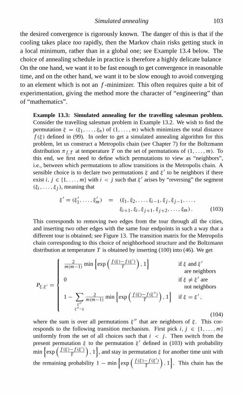
Simulated annealing 103
the desired convergence is rigorously known. The danger of this is that if thecooling takes placetoo rapidly, then the Markov chain risks getting stuck ina local minimum, rather than in a global one; see Example 13.4 below. Thechoice of annealing schedule in practice is therefore a highly delicate balance:On the one hand, we want it to be fast enough to get convergence in reasonabletime, and on the other hand, we want it to be slow enough to avoid convergingto an element which is not anf -minimizer. This often requires quite a bit ofexperimentation, giving the method more the character of “engineering” thanof “mathematics”.
Example 13.3: Simulated annealing for the travelling salesman problem.Consider the travelling salesman problem in Example 13.2. We wish to find thepermutationξ = (ξ1, . . . , ξn) of (1, . . . ,m) which minimizes the total distancef (ξ) defined in (99). In order to get a simulated annealing algorithm for thisproblem, let us construct a Metropolis chain (see Chapter 7) for the Boltzmanndistributionπ f,T at temperatureT on the set of permutations of(1, . . . ,m). Tothis end, we first need to define which permutations to view as “neighbors”,i.e., between which permutations to allow transitions in the Metropolis chain. Asensible choice is to declare two permutationsξ andξ ′ to be neighbors if thereexist i, j ∈ {1, . . . ,m} with i < j such thatξ ′ arises by “reversing” the segment(ξi , . . . , ξ j ), meaning that
ξ ′ = (ξ ′1, . . . , ξ
′m) = (ξ1, ξ2, . . . , ξi−1, ξ j , ξ j−1, . . . ,
ξi+1, ξi , ξ j+1, ξ j+2, . . . , ξm) . (103)
This corresponds to removing two edges from the tour through all the cities,and inserting two other edges with the same four endpoints in such a way that adifferent tour is obtained; see Figure 13. The transition matrix for the Metropolischain corresponding to this choice of neighborhood structure and the Boltzmanndistribution at temperatureT is obtained by inserting (100) into (46). We get
Pξ,ξ ′ =
2m(m−1) min
{exp
(f (ξ)− f (ξ ′)
T
),1
}if ξ andξ ′are neighbors
0 if ξ �= ξ ′ arenot neighbors
1−∑ξ ′′
ξ ′′∼ξ
2m(m−1) min
{exp
(f (ξ)− f (ξ ′′)
T
),1
}if ξ = ξ ′ ,
(104)where the sum is over all permutationsξ ′′ that are neighbors ofξ . This cor-responds to the following transition mechanism. First picki, j ∈ {1, . . . ,m}uniformly from the set of all choices such thati < j . Then switch from thepresent permutationξ to the permutationξ ′ defined in (103) with probabilitymin
{exp
(f (ξ)− f (ξ ′)
T
),1
}, and stay in permutationξ for another time unit with
the remaining probability 1− min{exp
(f (ξ)− f (ξ ′)
T
),1
}. This chain has the

104 13 Simulated annealing
1
89
10
11
313
12
7
4
214
5
6
1
89
10
11
313
12
7
4
214
5
6
Fig. 13. A transition in the Metropolis chain in Example 13.3 for thetravelling salesman problem, corresponding to going from the permutationξ = (1,2,3,4,5,6,7,8,9,10,11,12,13,14) to the permutation ξ ′ =(1,2,3,4,11,10,9,8,7,6,5,12,13,14).
Boltzmann distributionπ f,T as a reversible distribution, by the general Metropo-lis chain theory discussed in Chapter 7. The chain can also be shown to beirreducible (which is necessary in general for it to qualify as a useful MCMCchain).
It then only remains to decide upon a suitable cooling schedule, i.e., a suitablechoice of(T1, T2, . . .) and (N1, N2, . . .) in the simulated annealing algorithm.Unfortunately, we have no better suggestion than to do this by trial and error.
We note one very happy circumstance of the above example: When insertingthe Boltzmann distribution (100) into (46) to obtain (104), the normalizingconstantZ f,T cancelled everywhere, because all the expressions involving theBoltzmann distribution were in fact ratios between Boltzmann probabilities.That is very good news, because otherwise we would have had to calculateZ f,T , which is computationally infeasible. The same thing would happen forany Boltzmann distribution, and we therefore conclude that Metropolis chainsare in general very convenient tools for simulating Boltzmann distributions.Next, let us have a look at a simple example to warn against too rapid cooling
schedules.
Example 13.4: The hazard of using a fast annealing schedule.Let S ={s1, . . . , s4}, let f : S→ R be given by
f (s1) = 1f (s2) = 2f (s3) = 0f (s4) = 2
(105)

Simulated annealing 105
s4 s3
s2s1
Fig. 14. The graph structure chosen for the Metropolis algorithm in Example 13.4.
and suppose that we want to find the minimum off (si ) using simulated an-nealing.52 To find a Metropolis chain for the Boltzmann distribution onS attemperatureT , we need to impose a graph structure onS. Let’s say that we optfor the square formation in Figure 14. By applying (100) and (46), the transitionmatrix
1− e−1/T 1
2e−1/T 0 1
2e−1/T
12 0 1
2 00 1
2e−2/T 1− e−2/T 1
2e−2/T
12 0 1
2 0
is obtained. Suppose now that we run the inhomogeneous Markov chain(X0, X1, . . .) on S, corresponding to some given annealing schedule, startingwith X0 = s1. As in Footnote 51, writeT
(n) for the temperature at timen inthis annealing schedule. LetA be the event that the chain remains in states1forever (so that in particular the chain never finds thef -minimizing states3). Weget
P(A) = P(X1 = s1, X2 = s1, . . .)
= limn→∞P(X1 = s1, X2 = s1, . . . , Xn = s1)
= limn→∞P(X1 = s1 | X0 = s1)P(X2 = s1 | X1 = s1) · · ·×P(Xn = s1 | Xn−1 = s1)
= limn→∞
n∏i=1
(1− e−1/T (i )
)=
∞∏i=1
(1− e−1/T (i )
)
which is equal to 0 if and only if∑∞i=1 e−1/T
(i ) = ∞. Hence, ifT (n) is sent to
0 rapidly enough so that∑∞i=1 e−1/T
(i )< ∞, thenP(A) > 0, so that the chain
may get stuck in states1 forever. This happens, e.g., if we takeT(n) = 1
n . Thesimulated annealing algorithm then fails to find the true (global)f -minimizer f3.Two factors combine to create this failure, namely
(i) the annealing schedule being too fast, and
52 Of course, it is somewhat silly to use simulated annealing on a small problem like this one,where we can deduce that the minimum isf (s3) = 0 by immediate inspection of (105).This example is chosen just to give the simplest possible illustration of a phenomenon thatsometimes happens in simulated annealing algorithms for larger andmore interesting problems.

106 13 Simulated annealing
(ii) state s1 being a local f -minimizer (meaning thatf takes a smaller valueat s1 than at any of the neighbors ofs1 in the graph structure used for theMetropolis chain) without being a global one.
Let us give one final example of an optimization problem for which simulatedannealing may be a suitable method.
Example 13.5: Graph bisection.Given a graphG = (V, E) whose vertex setVcontains 2k vertices, the graph bisection problem is to find a way of partitioningV into two setsV1 andV2 with k elements each, such that the total number ofedges having one endpoint inV1 and the other inV2 is minimized. This problemis relevant for the design of search engines on the Internet:V may be the set ofall web pages on which a given word was found, edges represent links from onepage to another, and the hope is thatV1 andV2 will provide a relevant split intodifferent subareas.53 For instance, if the search word is “football”, then we mayhope thatV1 contains mostly pages about American football, andV2 mostly pagesabout soccer.
In recent years, several researchers haveabandoned the idea of an annealingschedule, and instead preferred to run the Metropolis chain at a single fixedtemperature, which is chosen on the basis of a careful mathematical analysisof the optimization problem at hand. For instance, Jerrum & Sorkin [JS] dothis for the graph bisection problem in Example 13.5. They show that forklarge and under reasonable assumptions on the input data, their algorithm finds,for arbitraryε > 0, the optimal bisection in timeCk2+ε with overwhelmingprobability ask → ∞, if T is taken to be of the ordern5/6+ε.
Problems13.1 (8) Modify the proof of Theorem 13.1 in order to take care of the case where
there are several elementss ∈ Ssatisfying f (s) = mins′∈S f (s′).13.2 (6) Describe a simulated annealing algorithm for the graph bisection problem in
Example 13.5. In particular, suggest a natural choice of neighborhood structurein the underlying Metropolis chain.
13.3 (8*) Suppose that we want to solve the optimal packing problem in Exam-ple 13.1 (i.e., we want to maximizef (ξ) over all feasible configurationsξ ∈{0,1}V , where f (ξ) is the number of 1’s inξ ), and decide to try simulatedannealing. To find suitable Markov chains, we start by considering Boltzmanndistributions for the functionf (ξ). Since we are dealing with a maximization(rather than minimization) problem, we considerthe modified Boltzmann distri-bution with the minus sign in the exponents of (100) and (101) removed.
(a) Show that this modified Boltzmann distribution at temperatureT is the same
as the probability measureµG,λ defined in Problem 7.4, withλ = exp(1T
).
53 In this application, it is of course also natural to relax the requirement thatV1 andV2 are ofequal size.

Simulated annealing 107
(b) Implement and run a simulated annealing algorithm for some suitable in-stances of this problem. (Note that due to (a), the MCMC algorithm con-structed in Problem 7.4 can be used for this purpose.)

14
Further reading
Markov theory is a huge subject (much bigger than indicated by these notes),and consequently there are many books written on it. Three books that haveinfluenced the present text are the ones by Bremaud [B], Grimmett & Stirzaker[GS], and (the somewhat more advanced book by) Durrett [Du]. Anothernice introduction to the topic is the book by Norris [N]. Some of my Swedishcompatriots will perhaps prefer to consult the texts by Ryden & Lindgren [RL]and Enger & Grandell [EG]. The reader can find plenty of additional material(more general theory, as wellas other directions for applications) in any ofthese references.Still on the Markov theory side (Chapters 2–6) of this text, there are two
particular topics that I would warmly recommend for further study to anyonewith a taste for mathematical elegance and the power and simplicity of prob-abilistic arguments: The first one isthe coupling method, which was usedto prove Theorems 5.2 and 8.1, and which also underlies the algorithms inChapters 10–12; see the books by Lindvall [L] and by Thorisson [T]. Thesecond topic is the relation betweenreversible Markov chains and electricalnetworks, which is delightfully treated in the book by Doyle & Snell [DSn].Haggstrom [H] gives a short introduction in Swedish.Another goldmine for the ambitiousstudent is the collection of papers edited
by Snell [Sn], where many exciting topics in probability, several of whichconcern Markov chains and/or randomized algorithms, are presented on a levelaccessible to advanced undergraduates.Moving on to the algorithmic side (Chapters 7–13), it is worth stressing
again that the collection of algorithms considered here in no way is represen-tative of the entire field of randomized algorithms. A reasonable overview canbe obtained by reading, in addition to these notes, the book by Motwani &Raghavan [MR]. See also the recent collection edited by Habib & McDiarmid[HM] for more on randomized algorithms and other topics at the interfacebetween probability and computer science.
108

Further reading 109
The main standard reference for MCMC (Chapter 7) these days seems tobe the the book edited by Gilks, Richardson & Spiegelhalter [GRS]. Anotherbook which is definitely worth reading is the research monograph by Sinclair[Si]. For the particular case of simulating the hard-core model describedin Example 7.1, see, e.g., the paper by Luby & Vigoda [LV]. The problemdiscussed in Chapter 8 of proving fast convergence of Markov chains has beenstudied by many authors. Some key references in this area are Diaconis & Fill[DF], Diaconis & Strook [DSt], Sinclair [Si] and Randall & Tetali [RT]; seealso the introductory paper by Rosenthal [R]. The treatment ofq-colorings inChapters 8 and 9 is based on the paper by Jerrum [J]. The general approach tocounting in Chapter 9 is treated nicely in [Si].Moving on to Propp–Wilson algorithms (Chapters 10–12), this is such a re-
cent topic that it has not yet been treated in book form. The original 1996 paperby Propp & Wilson [PW] has already become a classic, and should be read byanyone wanting to dig deeper into this topic. Other papers that may serveas introductions to the Propp–Wilson algorithm are those by Haggstrom &Nelander [HN] and Dimakos [Di]. An annotated bibliography on the subject,continuously maintained by Wilson, can be found at the web site [W2]. Fortreatments of the sandwiching technique of Chapter 11, see [PW] or any of theother references mentioned here. The subtle issue of exactly under what condi-tions (on the Markov chain) the sandwiching technique is applicableis treatedin a recent paper by Fill & Machida [FM]. The read-once variant of the Propp–Wilson algorithm considered in Chapter 12 was introduced by Wilson [W1].For the purpose of refining MCMCmethods in ways that lead to completely
unbiased samples, there is an interesting alternative to the Propp–Wilson al-gorithm that has become known asFill’s algorithm . It was introduced byFill [Fi], and then substantially generalized by Fill, Machida, Murdoch &Rosenthal [FMMR].For an introduction to the Ising model considered in Chapter 11 (and also to
some extent the hard-core model), see Georgii, Haggstrom & Maes [GHM].Concerning simulated annealing (Chapter 13), see the contribution by B. Gi-
das to the aforementioned collection [Sn]. Also worthy of attention is therecent emphasis on running the algorithm at a carefully chosen fixed tempera-ture; see Jerrum & Sorkin [JS].Finally, let me emphasize once more that the difficult problem of making
sure that we have access to a good (pseudo-)random number generator (asdiscussed very briefly in the beginning of Chapter 3) deserves serious attention.The classical reference for this problem is Knuth [K]. See also Goldreich[G] for an introduction to a promising new approach based on the theory ofalgorithmic complexity.

References
[B] Br emaud, P. (1998)Markov Chains: Gibbs fields, Monte Carlo Simula-tion, and Queues, Springer, New York.
[DF] Diaconis, P. & Fill, J. (1990) Strong stationary times via a new form ofduality,Annals of Probability18, 483–522.
[DSt] Diaconis, P. & Strook, D. (1991) Geometric bounds for eigenvalues ofMarkov chains,Annals of Applied Probability1, 36–61.
[Di] Dimakos, X.K. (2001) A guide to exact simulation,International Statis-tical Review69, 27–48.
[DSn] Doyle, P. & Snell, J.L. (1984)Random Walks and Electric Networks,Mathematical Monographs 22, Mathematical Association of Amer-ica.
[Du] Durrett, R. (1991)Probability: Theory and Examples, Wadsworth &Brooks/Cole, Pacific Grove.
[EG] Enger, J. & Grandell, J. (2000)Markovprocesser och Koteori, Mathe-matical Statistics, KTH, Stockholm.
[Fa] Fagin, R., Karlin, A., Kleinberg, J., Raghavan, P., Rajagopalan, S.,Rubinfeld, R., Sudan, M. & Tomkins, A. (2000) Random walks with“back buttons”,Proceedings of the 32nd Annual ACM Symposium onTheory of Computing, Portland, Oregon, pp. 484–493.
[Fi] Fill, J. (1998) An interruptible algorithm for perfect sampling via Markovchains,Annals of Applied Probability8, 131–162.
[FM] Fill, J. & Machida, M. (2001) Stochastic monotonicity and realizablemonotonicity,Annals of Probability,29, 938–978.
[FMMR] Fill, J., Machida, M., Murdoch, D. & Rosenthal, J. (2000) Exten-sion of Fill’s perfect rejection sampling algorithm to general chains,Random Structures and Algorithms17, 290–316.
110

References 111
[GG] Geman, S. & Geman, D. (1984) Stochastic relaxation, Gibbs distribu-tions, and the Bayesian restoration of images,IEEE Transactions onPattern Analysis and Machine Intelligence6, 721–741.
[GHM] Georgii, H.-O., Haggstrom, O. & Maes, C. (2001) The randomgeometry of equilibrium phases,Phase Transitions and Critical Phe-nomena, Volume 18(C. Domb & J.L. Lebowitz, eds), pp. 1–142,Academic Press, London.
[GRS] Gilks, W., Richardson, S. & Spiegelhalter, D. (1996)Markov ChainMonte Carlo in Practice, Chapman & Hall, London.
[G] Goldreich, O. (1999) Pseudorandomness,Notices of the American Math-ematical Society46, 1209–1216.
[GS] Grimmett, G. & Stirzaker, D. (1992)Probability and Random Pro-cesses, Clarendon, Oxford.
[HM] Habib, M. & McDiarmid, C. (2000)Probabilistic Methods for Algo-rithmic Discrete Mathematics, Springer, New York.
[H] Haggstrom, O. (2000) Slumpvandringar och likstromskretsar,Elementa83, 10–14.
[HN] Haggstrom, O. & Nelander, K. (1999) On exact simulation of Markovrandom fields using coupling from the past,Scandinavian Journal ofStatistics26, 395–411.
[J] Jerrum, M. (1995) A very simplealgorithm for estimating the number ofk-colorings of a low-degree graph,Random Structures and Algorithms7, 157–165.
[JS] Jerrum, M. & Sorkin, G. (1998) The Metropolis algorithm for graphbisection,Discrete Applied Mathematics82, 155–175.
[K] Knuth, D. (1981)The Art of Computer Programming. Volume 2. Seminu-merical Algorithms, 2nd edition, Addison–Wesley, Reading.
[L] Lindvall, T. (1992)Lectures on the Coupling Method, Wiley, New York.[LV] Luby, M. & Vigoda, E. (1999) Fast convergence ofthe Glauber dynam-
ics for sampling independent sets,Random Structures and Algorithms15, 229–241.
[MR] Motwani, R. & Raghavan, P. (1995)Randomized Algorithms, Cam-bridge University Press.
[N] Norris, J. (1997)Markov Chains, Cambridge University Press.[PW] Propp J. & Wilson, D. (1996) Exact sampling with coupled Markov
chains and applications to statistical mechanics,Random Structuresand Algorithms9, 232–252.
[RT] Randall, D. & Tetali, P. (2000) Analyzing Glauber dynamics by compar-ison of Markov chains,Journal of Mathematical Physics41, 1598–1615.

112 References
[R] Rosenthal, J. (1995) Convergence rates for Markov chains,SIAM Review37, 387–405.
[RL] Ryden, T. & Lindgren, G. (1996)Markovprocesser, Lunds Universitetoch Lunds Tekniska Hogskola, Institutionen for matematisk statistik.
[Si] Sinclair, A. (1993)Algorithms for Random Generation and Counting. AMarkov Chain Approach, Birkhauser, Boston.
[Sn] Snell, J.L. (1994)Topics in Contemporary Probability and its Applica-tions, CRC Press, Boca Raton.
[T] Thorisson, H. (2000)Coupling, Stationarity, and Regeneration, Springer,New York.
[W1]Wilson, D. (2000) How to couple from the past using a read-once sourceof randomness,Random Structures and Algorithms16, 85–113.
[W2] Wilson, D. (2001) Perfectly random sampling with Markov chains,http://dimacs.rutgers.edu/˜dbwilson/exact.html/

Index
annealing schedule, 102, 104aperiodicity, 25
Bernoulli (p) random variable, 6binomial(n, p) random variable, 6, 43, 71birth-and-death process, 41, 92Boltzmann distribution, 100
Chebyshev’s inequality, 6, 71, 74chess, 27, 43coin tossing, 8, 71, 96conditional probability, 2counting problem, 64coupling, 34, 57, 62, 76, 81, 94
density, 3distribution, 3
Ehrenfest’s urn model, 43equilibrium, 28, 34expectation, 4
Fill’s algorithm, 109four-color theorem, 49
geometric distribution, 96Gibbs sampler, 49graph, 40graph bisection, 106
hard-core model, 45, 47, 52, 99hitting time, 29homogeneity, 10
i.i.d. (independent and identically distributed),3
independence, 2indicator function, 18
inhomogeneous Markov chain, 13, 50, 100initial distribution, 10initiation function, 18Internet, 13, 52, 106irreducibility, 23Ising model, 87
ladder walk, 85Law of Large Numbers, 7, 68, 69, 88
Markov chain, 10Markov property, 9MCMC (Markov chain Monte Carlo), 47mean, 4memoryless property, 9Metropolis chain, 50
optimal packing, 99
perfect simulation, 76phase transition, 88polynomial time algorithm, 65polynomial time approximation scheme, 66probability measure, 1Propp–Wilson algorithm, 76
randomq-coloring, 49random number generator, 17, 109random variable, 2random walk, 8, 40reversibility, 39, 48, 51
simulated annealing, 100St Petersburg paradox, 4stationary distribution, 28, 34, 37, 39, 47Steiner’s formula, 5systematic sweep Gibbs sampler, 50, 55
113

114 Index
total variation distance, 33, 38, 62transition graph, 13transition matrix, 10travelling salesman problem, 99
uniform [0,1] random variable, 4update function, 19
Wilson’s modification, 94