finite element method. stability and eigenfrequenciesstaff.iha.dk/lc/fem/fem_noter/civil/bk101.2...

Finite Element Method. Stability and eigenfrequenciesmarts 2017/LC

1


FEM calculation of critical loads and eigenfrequencys.

I these notes stability is flexural buckling of compressed structure elements.Instability as buckling of shells and lateral torsional buckling of beams and columns can be treated after the same principles, but this is not included in these notes.Regarding buckling of shells and lateral torsional buckling of beams and columns, it is usually necessary to make a full 3D model of the structure in shell elements. Finite Element theory is used as the basic theory of the topics.

Contents:

2


Symbols

Stiffness_matrix ЌGeometric_stiffness_matrix Ќσ

Mass_matrix ЌmEigenvalue λ

Displacement u

Rotation r

Deformation_vector ūLength L

Modulus_of_elasticity E

Moment_of_inertia I

⎡⎢⎢⎢⎢⎢⎢⎢⎢⎢⎢⎢⎣

⎤⎥⎥⎥⎥⎥⎥⎥⎥⎥⎥⎥⎦

3


1.0 FEM calculation of forces and deformations for beams.

1.1 Shape functions: Shape functions is the mathematical approximations which describe a deformation of a beam for different impacts. En horizontal beam has 4 degrees of freedom and therefore also 4 shape functions:

A vertical displacement in the left end of the beam.ϕ1 ((x))A torsion of the left end of the beam.ϕ2 ((x))A vertical displacement in the right end of the beam.ϕ3 ((x))A torsion of the right end of the beam.ϕ4 ((x))

Excluding normal forces and horizontal movements, as they are addressed under the topic bars

A shape function can assume all values between 0 or 1.When one shape function has the value 1, all the other shape functions has the value 0.If shape function has the value 1, the torsion angel is 1 in the left end. ϕ2 ((x))The shape functions , and will then take the value 0 ϕ1 ((x)) ϕ3 ((x)) ϕ4 ((x))

The approximations for the shape functions is shown below.

1.1 Shape functions.

＝ϕ1 ((x)) +-⋅2⎛⎜⎝―x

L

⎞⎟⎠

3

⋅3⎛⎜⎝―x

L

⎞⎟⎠

2

1 ＝ϕ2 ((x)) ⋅-x⎛⎜⎝

+-⎛⎜⎝―x

L

⎞⎟⎠

2

⋅2 ―x

L1⎞⎟⎠

＝ϕ3 ((x)) +⋅-2⎛⎜⎝―x

L

⎞⎟⎠

3

⋅3⎛⎜⎝―x

L

⎞⎟⎠

2

＝ϕ4 ((x)) ⋅-x⎛⎜⎝

-⎛⎜⎝―x

L

⎞⎟⎠

2

―x

L

⎞⎟⎠

Shape functions graphically:

Figure 1

4


Developing of the shape functions. Shape function 1:

As shown in the Figure s all shape functions has a turning tangent and therefore assumed to have anapproximation as a 3rd degree polynomial: . The boundary conditions for ＝ϕ1 +++⋅A x3 ⋅B x2 ⋅C x D

this polynomial is: u1=1 for x=0. u2=0 for x=L. =0 for x=0 and x=L.――d

dxϕ1

1) . => D=1.＝+++⋅A 03 ⋅B 02 ⋅C 0 D 12) . ＝+++⋅A L3 ⋅B L2 ⋅C L D 03) . => C=0＝++⋅⋅3 A 02 ⋅⋅2 B 0 ⋅C 0 0

4) . => ＝+⋅⋅3 A L2 ⋅⋅2 B L 0 ＝A ―――⋅-2 B

⋅3 L

2) . => . => . And finally:＝++⋅―――⋅-2 B

⋅3 LL3 ⋅B L2 1 0 ＝B ――

-3

L2＝A ――

2

L3

. The above approximation for shape function 1 is now proven. The other ＝ϕ1 +-⋅2⎛⎜⎝―x

L

⎞⎟⎠

3

⋅3⎛⎜⎝―x

L

⎞⎟⎠

2

1

shape functions can be found in a similar way.

The stiffness matrix for one element:

＝Ќ ⋅――⋅E I

L3

12 ⋅-6 L -12 ⋅-6 L

⋅-6 L ⋅4 L2 ⋅6 L ⋅2 L2

-12 ⋅6 L 12 ⋅6 L

⋅-6 L ⋅2 L2 ⋅6 L ⋅4 L2

⎡⎢⎢⎢⎢⎣

⎤⎥⎥⎥⎥⎦

As shown later on, the stiffness matrix can be developed from the shape functions:i and j are the number of the shape function referring to number of roe and column in the stiffnessmatrix.

＝＝Kij ⋅⋅E I⌠⎮⌡ d0

L

⋅φ''iTφ''j x ⋅⋅E I

⌠⌡ d0

L

⋅B TB x

1.2 Sign convention while calculation forces in the nodes:To make it possible to add two beams elements simply, we consider the following signs convention..

Sign convention when drawing shear force diagrams and bending moment diagram.1.2.1 Traditional convention of signs:

Figure 2. Sign convention when drawing shear force diagrams and bending moment diagram.

1.2.1 Traditional convention of signs 1.2.2 FEM. Sign convention when calculation the forces

5


Usually the differential equation for beams looks like this: . ＝――⋅d2 u

dx2――-M

⋅E I

With our new sign convention, the differential equation for beams looks like this: ＝――⋅d2 u

dx2――M

⋅E I

1.3 Stiffness matrix from the principle of virtual work:

Figure 3

u is the displacement. will be the torsion angle. ――du

dx

Arc length is close to = . . l ((x)) ⋅y ―――du ((x))

dx

＝l ((x)) ⋅y ―――du ((x))

dxstrain ＝ε ――

dl ((x))

dx

＝＝ε ⋅y ――d

d

2

x2u ((x)) ⋅y ――

d

d

2

x2(( ⋅ϕ ((x)) u)) ＝ε ⋅⋅y B ((x)) ū

ε is a vector with four components.The internal work:

＝Ai⌠⌡ d⋅Tε σ v v is the volume ＝σ ⋅E ε ＝＝Ai

⌠⌡ d⋅⋅Tε E ε v

⌠⌡ d⋅⋅⋅⋅⋅⋅y TB Tū E y B ū v

The external work from the distributed load: ＝＝Ays ⌠⌡ d⋅u ((x)) p ((x)) x ⌠

⌡ d⋅⋅ϕ ((x)) ū p ((x)) x

The external work from forces and moments: ＝＝Ayn ⋅Tū Pe ⋅Tū P1 M1 P2 M2[[ ]]

＝Ai +Ays Ayn ＝⌠⌡ d⋅⋅⋅⋅⋅⋅y TB Tū E y B ū v +

⌠⎮⌡ d⋅⋅

Tϕ ((x)) Tū p ((x)) x ⋅Tū P1 M1 P2 M2[[ ]]

⇒ ＝⋅Tū ⌠⌡ d⋅⋅⋅⋅y2 TB E B ū v +⋅Tu

⌠⎮⌡ d⋅

Tϕ ((x)) p ((x)) x ⋅Tū P1 M1 P2 M2[[ ]]

⇒ ＝⋅⋅⋅⌠⌡ dy2 A E

⌠⌡ d⋅T((B)) B x ū +

⌠⎮⌡ d⋅

T((ϕ ((x)))) p ((x)) x P1 M1 P2 M2[[ ]]

⇒ ＝⋅⋅⋅E I⌠⌡ d⋅T((B)) B x ū +

⌠⎮⌡ d⋅

T((ϕ ((x)))) p ((x)) x Pe ⇒ ＝⋅Ќ ū Ū ⇒ ＝K ⋅⋅E I

⌠⌡ d⋅T((B)) B x

K - matrix:＝Ќ ⋅――

⋅E I

L3

12 ⋅-6 L -12 ⋅-6 L

⋅-6 L ⋅4 L2 ⋅6 L ⋅2 L2

-12 ⋅6 L 12 ⋅6 L

⋅-6 L ⋅2 L2 ⋅6 L ⋅4 L2

⎡⎢⎢⎢⎢⎣

⎤⎥⎥⎥⎥⎦

＝Ќij ⋅⋅E I⌠⎮⌡ d0

L

⋅T

B1 B2 B3 B4[[ ]] B1 B2 B3 B4[[ ]] x

6


Example. Value in 2. row, 3. column:

＝K23⌠⌡ d0

L

⋅⋅ϕ''2 EI ϕ''3 x

⇒ ＝⌠⎮⎮⌡

d

0

L

⋅⋅⋅⎛⎜⎜⎝――d

d

2

x2

⎛⎜⎝

⋅-x⎛⎜⎝

+-⎛⎜⎝―x

L

⎞⎟⎠

2

⋅2 ―x

L1⎞⎟⎠

⎞⎟⎠

⎞⎟⎟⎠E I ――

d

d

2

x2

⎛⎜⎝

+⋅-2⎛⎜⎝―x

L

⎞⎟⎠

3

⋅3⎛⎜⎝―x

L

⎞⎟⎠

2 ⎞⎟⎠

x ―――⋅⋅6 E I

L2

1.4 Example. Cantilever beam IPE-240 with a vertical force:

≔Pb ⋅10 kN ≔L ⋅5 m ≔I ⋅⋅38.9 106 mm 4 ≔E ⋅⋅2.1 105 ――N

mm2

Results with traditional sign convention as e.g. Teknisk Ståbi:

≔Ma ⋅-Pb L ≔Va -Pb ≔ub ―――⋅Pb L3

⋅⋅3 E I≔rb ―――

⋅-Pb L2

⋅⋅2 E I

=Ma -50 ⋅kN m ≔Ra ⋅104 kN =ub 51.006 mm =rb -0.015

Pb

Figure 4Results from the FEM calculation:

＝Ќ ⋅――⋅E I

L2

―12

L-6 -―

12

L-6

-6 ⋅4 L 6 ⋅2 L

-―12

L6 ―

12

L6

-6 ⋅2 L 6 ⋅4 L

⎡⎢⎢⎢⎢⎢⎢⎣

⎤⎥⎥⎥⎥⎥⎥⎦

＝ū

00ubrb

⎡⎢⎢⎢⎢⎣

⎤⎥⎥⎥⎥⎦

＝Ū

Ra.

Ma

Pb0

⎡⎢⎢⎢⎢⎣

⎤⎥⎥⎥⎥⎦

The first 2 rows in u is 0. Then the 2 first columns and rows in the K-matrix can be taken out.This results in a modified system:

＝Ќmod ⋅――⋅E I

L2

―12

L6

6 ⋅4 L

⎡⎢⎢⎣

⎤⎥⎥⎦

＝ūmodubrb

⎡⎢⎣

⎤⎥⎦

＝ŪmodPb0

⎡⎢⎣

⎤⎥⎦

＝ūmod ⋅Ќmod-1 Ūmod

＝＝ubrb

⎡⎢⎣

⎤⎥⎦

⋅

⎛⎜⎜⎝

⋅――⋅E I

L2

―12

L6

6 ⋅4 L

⎡⎢⎢⎣

⎤⎥⎥⎦

⎞⎟⎟⎠

-1

Pb0

⎡⎢⎣

⎤⎥⎦

⋅⋅―1

3――L3

⋅E IPb

⋅⋅―――-1

⋅2 ⋅E IL2 Pb

⎡⎢⎢⎢⎢⎣

⎤⎥⎥⎥⎥⎦

⇒ ＝⋅⋅―

1

3――L3

⋅E IPb

⋅⋅―――-1

⋅2 ⋅E IL2 Pb

⎡⎢⎢⎢⎢⎣

⎤⎥⎥⎥⎥⎦

⋅51.01 mm

-0.02⎡⎢⎣

⎤⎥⎦

7


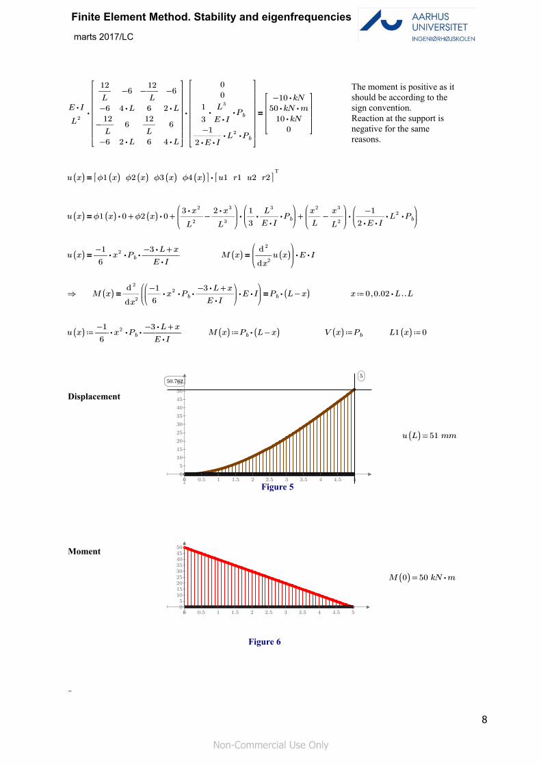
The moment is positive as it should be according to the sign convention.Reaction at the support is negative for the same reasons.

＝⋅⋅――⋅E I

L2

―12

L-6 -―

12

L-6

-6 ⋅4 L 6 ⋅2 L

-―12

L6 ―

12

L6

-6 ⋅2 L 6 ⋅4 L

⎡⎢⎢⎢⎢⎢⎢⎣

⎤⎥⎥⎥⎥⎥⎥⎦

00

⋅⋅―1

3――L3

⋅E IPb

⋅⋅―――-1

⋅2 ⋅E IL2Pb

⎡⎢⎢⎢⎢⎢⎢⎢⎣

⎤⎥⎥⎥⎥⎥⎥⎥⎦

⋅-10 kN

⋅⋅50 kN m

⋅10 kN

0

⎡⎢⎢⎢⎣

⎤⎥⎥⎥⎦

＝u ((x)) ⋅ϕ1 ((x)) ϕ2 ((x)) ϕ3 ((x)) ϕ4 ((x))[[ ]]T

u1 r1 u2 r2[[ ]]

＝u ((x)) +++⋅ϕ1 ((x)) 0 ⋅ϕ2 ((x)) 0 ⋅⎛⎜⎜⎝

-――⋅3 x2

L2――⋅2 x3

L3

⎞⎟⎟⎠

⎛⎜⎝

⋅⋅―1

3――L3

⋅E IPb⎞⎟⎠

⋅⎛⎜⎜⎝

-――x2

L――x3

L2

⎞⎟⎟⎠

⎛⎜⎝

⋅⋅―――-1

⋅2 ⋅E IL2 Pb

⎞⎟⎠

＝u ((x)) ⋅⋅⋅――-1

6x2 Pb ――――

+⋅-3 L x

⋅E I＝M ((x)) ⋅⋅⎛⎜⎜⎝――d

d

2

x2u ((x))

⎞⎟⎟⎠E I

⇒ ＝＝M ((x)) ――d

d

2

x2

⎛⎜⎝

⋅⋅⎛⎜⎝

⋅――-1

6⋅x

2 ⋅Pb ――――+⋅-3 L x

⋅E I

⎞⎟⎠E I

⎞⎟⎠

⋅Pb (( -L x)) ≔x , ‥0 ⋅0.02 L L

≔u ((x)) ⋅⋅⋅――-1

6x2 Pb ――――

+⋅-3 L x

⋅E I≔M ((x)) ⋅Pb (( -L x)) ≔V ((x)) Pb ≔L1 ((x)) 0

10

15

20

25

30

35

40

45

50

0

5

55

1 1.5 2 2.5 3 3.5 4 4.50 0.5 5

50.7625

Displacement

=u ((L)) 51 mm

Figure 5

1015202530354045

05

50

1 1.5 2 2.5 3 3.5 4 4.50 0.5 5

Moment

=M ((0)) 50 ⋅kN m

Figure 6

¨

8


23456789

01

10

1 1.5 2 2.5 3 3.5 4 4.50 0.5 5

Shear forces=V ((0)) 10 kN

Figure 7

1.5 Global coordinates.If the structure elements are rotated with an angle to one another, it is necessary to transform the stiffness matrix in to a global system, which is the same for all elements in the structure.

Figure 8

To transform the stiffness matrixes in to a global system, it is necessary to include all forces in the beams, shear forces normal forces and moments.

Global stiffness matrix. Global geometric stiffness matrix.

＝Ke ⋅――⋅E I

L3

⋅―A

IL2 0 0 ⋅-―

A

IL2 0 0

0 12 ⋅-6 L 0 -12 ⋅-6 L

0 ⋅-6 L ⋅4 L2 0 ⋅6 L ⋅2 L2

⋅-―A

IL2 0 0 ⋅―

A

IL2 0 0

0 -12 ⋅6 L 0 12 ⋅6 L

0 ⋅-6 L ⋅2 L2 0 ⋅6 L ⋅4 L2

⎡⎢⎢⎢⎢⎢⎢⎢⎢⎢⎣

⎤⎥⎥⎥⎥⎥⎥⎥⎥⎥⎦

＝Keσ ⋅――N

⋅30 L

0 0 0 0 0 00 36 ⋅-3 L 0 -36 ⋅-3 L

0 ⋅-3 L ⋅4 L2 0 ⋅3 L -L2

0 0 0 0 0 00 -36 ⋅3 L 0 36 ⋅3 L

0 ⋅-3 L -L2 0 ⋅3 L ⋅4 L2

⎡⎢⎢⎢⎢⎢⎢⎣

⎤⎥⎥⎥⎥⎥⎥⎦

The stiffness matrix for both elements can be transformedwith a transformation matrix. Of course the angles is different for the two elements shown in the Figure above.v1 = π/2 and v2 = 0.

＝T

cos ((v)) sin ((v)) 0 0 0 0-sin ((v)) cos ((v)) 0 0 0 0

0 0 1 0 0 00 0 0 cos ((v)) sin ((v)) 00 0 0 -sin ((v)) cos ((v)) 00 0 0 0 0 1

⎡⎢⎢⎢⎢⎢⎢⎣

⎤⎥⎥⎥⎥⎥⎥⎦

Global transformation matrix.

＝K ⋅⋅TT Ke T ＝Kσ ⋅⋅T

T Keσ T

9


1.6 Distributed loads.

If the structure has a distributed load, the procedure for calculating forces and deformation will be a little more complicated. The distributed load has to be transformed to equivalent nodal forces in the nodes, before computing the deformations.When afterward computing the reactions, the virtual load must be taken out of the calculation to determine the reactions.

Figure 9

The shown distributed load can be written as: ＝p ((x)) ⋅p ―x

L

The equivalent nodal forces will be determined from the shape functions:

. In this example the equivalent nodal forces will affect only element 2.＝EUi⌠⌡ d⋅ϕi p ((x)) x

For the first equivalent nodal forces, which is the vertical load in B:

＝＝EU1

⌠⎮⎮⌡

d

0

L

⋅⋅⎛⎜⎜⎝

+-1 ――⋅3 x2

L2――⋅2 x3

L3

⎞⎟⎟⎠p ―

x

Lx ⋅⋅―

3

20L P

The next equivalent nodal force, witch is the bending moment in B:

＝＝EU2

⌠⎮⎮⌡

d

0

L

⋅⋅-⎛⎜⎜⎝

+-x ――⋅2 x2

L――x3

L2

⎞⎟⎟⎠p ―

x

Lx ⋅⋅――

-1

30L2 p

In similar way, we can find the equivalent forces in C:

＝＝EU3

⌠⎮⎮⌡

d

0

L

⋅⋅⎛⎜⎜⎝

-――⋅3 x2

L2――⋅2 x3

L3

⎞⎟⎟⎠p ―

x

Lx ⋅⋅―

7

20L p

＝＝EU4

⌠⎮⎮⌡

d

0

L

⋅⋅⎛⎜⎜⎝

-――x2

L――x3

L2

⎞⎟⎟⎠p ―

x

Lx ⋅⋅―

1

20L2 p

To find the deformations we look at the following equation: . From the ＝⋅Ќ ū +Ū EŪreduced modified system, we find the deformations: .＝ūmod ⋅Ќmod

-1 ⎛⎝ +Ūmod EŪmod⎞⎠

Finally the reactions can be found: . ＝Ū -⋅Ќ ū EŪ

10


2.0 FEM calculation for the critical load for a bar.

2.1 The geometric stiffness matrix derived using the direct method.A thin rod or bar has a relatively low stiffness against deformation perpendicular to the longitudinal direction. If the rod is applied to a normal force, the stiffness against lateral deflection will be changed. If the normal force is tension, the stiffness against shear strain perpendicular to the rods longitudinal direction will become larger. Conversely, a compressive axial force rod quickly render unstable. The geometricstiffness matrix that tells something about the influence of a normal force has on the deformations and stiffness perpendicular to the longitudinal axis. The geometric stiffness matrix can be derived in 2 ways. A static view and a mathematical consideration. We start with the static view of a rod. Figure 1 shows a deformed rod supported by springs in all charniers and Figure 2 shows a section of the deformed bar here with a normal force.

2.2 Bars. The direct method.

Figure 10

Figure 11

Vertical projection: ＝F1 -F2

Moment in pt. 2 on Figure 11: ＝⋅F1 L ⋅N (( -u1 u2))

⇒ ＝F1

F2

⎡⎢⎣

⎤⎥⎦

⋅⋅―N

L

1 -1-1 1⎡⎢⎣

⎤⎥⎦

u1

u2

⎡⎢⎣

⎤⎥⎦

Moment in pt. 1 on Figure 11: ＝⋅F2 L ⋅N (( -u2 u1))

This shows a connection between normal forces and deformations perpendicular to the length axe.

11


2.3 Beams. The direct method.

For a beam the same method can be considered:

Figure 12

Again one can establish some equilibrium equations, however this becomes somewhat more complicated because of the now occurring moments and rotations. The system is statically indeterminate, and it's a little complicated to deduce the geometric stiffness matrix in this way. By using equilibrium equations one can with difficulty find all the terms in the geometric stiffness matrix that looks as shown below. Note that material values and cross sections values are not included in this term. On the other hand, a relationship between normal forces and geometry of the beam is expressed:

＝Ќσ ⋅――N

⋅30 L

36 ⋅-3 L -36 ⋅-3 L

⋅-3 L ⋅4 L2 ⋅3 L -L2

-36 ⋅3 L 36 ⋅3 L

⋅-3 L -L2 ⋅3 L ⋅4 L2

⎡⎢⎢⎢⎢⎣

⎤⎥⎥⎥⎥⎦

＝⋅⋅――N

⋅30 L

36 ⋅-3 L -36 ⋅-3 L

⋅-3 L ⋅4 L2 ⋅3 L -L2

-36 ⋅3 L 36 ⋅3 L

⋅-3 L -L2 ⋅3 L ⋅4 L2

⎡⎢⎢⎢⎢⎣

⎤⎥⎥⎥⎥⎦

u1r1u2r2

⎡⎢⎢⎢⎢⎣

⎤⎥⎥⎥⎥⎦

F1

M1

F2

M2

⎡⎢⎢⎢⎣

⎤⎥⎥⎥⎦

2.4 Beams. The geometric stiffness matrix derived from the principle of virtual work.

Figure 13

The force N will because of the virtual deformations (angle v) come closer to one another by the distance ddx. From the geometry is seen, that the angle which create the displacement ddx must be ½·v.

＝v ――du

dx⇒ ＝ddx ⋅du ―

v

2 The vertical displacement can be expressed as ⋅――du

dxdx

12


⇒ ＝ddx ⋅⋅⋅―1

2――du

dx――du

dxdx The external work is: ＝Wy ⋅⋅N ―

1

2

⌠⎮⎮⌡

d⋅――du

dx――du

dxx

Displacement can be written as: . Using the ＝u ((x)) +++a1 ⋅a2 x ⋅a3 x2 ⋅a4 x3

shape functions:or . The external work is now:＝u ((x)) +++⋅u1 ϕ1 ⋅r1 ϕ2 ⋅u2 ϕ3 ⋅r2 ϕ4 ＝u ((x)) ⋅ϕ ū.

＝Ay ⋅―1

2

⌠⎮⎮⌡

d⋅⋅⋅⋅――Tdϕi

dx

Tū N ――dϕj

dxū x

The geometric stiffness matrix is defined by: ＝Kσ.ij

⌠⎮⎮⌡

d⋅⋅――Tdϕi

dxN ――

dϕj

dxx

＝Kσ23

⌠⌡ d0

L

⋅⋅ϕ'2 N ϕ'3 x ⇒ ＝⌠⎮⎮⌡

d

0

L

⋅⋅⎛⎜⎜⎝――d

d

1

x1

⎛⎜⎝

⋅-x⎛⎜⎝

+-⎛⎜⎝―x

L

⎞⎟⎠

2

⋅2 ―x

L1⎞⎟⎠

⎞⎟⎠

⎞⎟⎟⎠N ――

d

d

1

x1

⎛⎜⎝

+⋅-2⎛⎜⎝―x

L

⎞⎟⎠

3

⋅3⎛⎜⎝―x

L

⎞⎟⎠

2 ⎞⎟⎠

x ―N

10

＝Ќσ ⋅――N

⋅30 L

36 ⋅-3 L -36 ⋅-3 L

⋅-3 L ⋅4 L2 ⋅3 L -L2

-36 ⋅3 L 36 ⋅3 L

⋅-3 L -L2 ⋅3 L ⋅4 L2

⎡⎢⎢⎢⎢⎣

⎤⎥⎥⎥⎥⎦

2.5 Principle of virtual work for flexural buckling of columns: ＝Ay Ai

FEM equation, which contain forces and reactions: . This equation is also used for finding shear ＝⋅Ќ ū Ūforces and moments. If these forces is multiplied with the corresponding deformations we have the internal work . Where is the virtual deformations.＝Ai ⋅⋅Tūv Ќ ū. ūv

Performing buckling analysis, it is important to divide the structure parts in to smaller elements. Typically a column is divided in to 10 elements.The nodes in the elements will because of the normal force get a displacement perpendicular to the length of the column, as determined in the geometric stiffness matrix.The multiplication of forces in the nodes and the corresponding deformations will be the external work:

.＝Ay ⋅⋅Tūv Ќσ ū

＝Ai Ay ⇒ ＝⋅⋅Tūv Ќ ū ⋅⋅⋅λ Tūv Ќσ ū ⇒ ＝⋅⋅Tūv ⎛⎝ -Ќ ⋅λ Ќσ⎞⎠ ū 0

We are looking for a condition fore fulfilling the principle of virtual work.To find this condition we can regulate the normal force until .＝Ay Ai

This can be done by multiplying a factor to the normal force and therefore to the external work.The result shall be valid for any virtual deformation, so can be divided out of the system:ūv

. is determined from the reduced modified system.＝⋅⎛⎝ -Ќ ⋅λ Ќσ⎞⎠ ū 0 ūWe now have a reduced system of equations. Mathematically this is a linear eigenvalue problem, which according to Cramer's Rule can be solved from the equation: . ＝|| -Ќ ⋅λ Ќσ|| 0

13


2.6 Cramer's rule.

＝Ќ a1 a2

a3 a4

⎡⎢⎣

⎤⎥⎦

＝Ќσb1 b2

b3 b4

⎡⎢⎣

⎤⎥⎦

＝ū u1

u2

⎡⎢⎣

⎤⎥⎦

＝⋅⎛⎝ -Ќ ⋅λ Ќσ⎞⎠ ū 0 ⇒

＝⋅⎛⎜⎝

-a1 a2

a3 a4

⎡⎢⎣

⎤⎥⎦

⋅λb1 b2

b3 b4

⎡⎢⎣

⎤⎥⎦

⎞⎟⎠

u1

u2

⎡⎢⎣

⎤⎥⎦

0 ⇒ ＝⋅-a1 ⋅λ b1 -a2 ⋅λ b2

-a3 ⋅λ b3 -a4 ⋅λ b4

⎡⎢⎣

⎤⎥⎦

u1

u2

⎡⎢⎣

⎤⎥⎦

00⎡⎢⎣

⎤⎥⎦

This equation can be satisfied by u1 = u2 = 0, which is not the only workable solution.

If u1 = u2 is not supposed to be 0, it is necessary that the rows in the matrix: are -a1 ⋅λ b1 -a2 ⋅λ b2

-a3 ⋅λ b3 -a4 ⋅λ b4

⎡⎢⎣

⎤⎥⎦

proportional:

＝――――-a1 ⋅λ b1

-a3 ⋅λ b3――――

-a2 ⋅λ b2

-a4 ⋅λ b4⇒ ＝-⋅(( -a1 ⋅λ b1)) (( -a4 ⋅λ b4)) ⋅(( -a2 ⋅λ b2)) (( -a3 ⋅λ b3)) 0

This equation is exactly the same equation as we get by setting the determinant for -a1 ⋅λ b1 -a2 ⋅λ b2

-a3 ⋅λ b3 -a4 ⋅λ b4

⎡⎢⎣

⎤⎥⎦

to 0.The equation has one solution: .＝⋅⎛⎝ -Ќ ⋅λ Ќσ⎞⎠ ū 0 ＝|| -Ќ ⋅λ Ќσ|| 0

By computing this determinant appears as the unknown. The result is the factor to be multiplied to the λ

current axial load, thus there is an equilibrium.The critical load, for example a search column with normal force N is therefore ·N.λ

14


2.7 Example with column 1.

15


2.7.1 Column 1. Solution with 2 elements. L as shown on the Figure.

＝Ќ ⋅⋅E I

――12

L3

-――6

L2

――-12

L3

-――6

L2

0 0

-――6

L2―4

L――6

L2―2

L0 0

――-12

L3――6

L2――24

L30 ――

-12

L3-――6

L2

-――6

L2―2

L0 ―

8

L――6

L2―2

L

0 0 ――-12

L3――6

L2――12

L3――6

L2

0 0 -――6

L2―2

L――6

L2―4

L

⎡⎢⎢⎢⎢⎢⎢⎢⎢⎢⎢⎢⎢⎢⎢⎢⎢⎣

⎤⎥⎥⎥⎥⎥⎥⎥⎥⎥⎥⎥⎥⎥⎥⎥⎥⎦

＝Ќσ ⋅P

――6

⋅5 L――-1

10――-6

⋅5 L――-1

100 0

――-1

10――⋅2 L

15―1

10⋅――

-1

30L 0 0

――-6

⋅5 L―1

10――12

⋅5 L0 ――

-6

⋅5 L――-1

10

――-1

10⋅――

-1

30L 0 ――

⋅4 L

15―1

10⋅――

-1

30L

0 0 ――-6

⋅5 L―1

10――6

⋅5 L―1

10

0 0 ――-1

10⋅――

-1

30L ―

1

10――⋅2 L

15

⎡⎢⎢⎢⎢⎢⎢⎢⎢⎢⎢⎢⎢⎢⎢⎢⎣

⎤⎥⎥⎥⎥⎥⎥⎥⎥⎥⎥⎥⎥⎥⎥⎥⎦

Boundary conditions:which means that 1., 4. and 5. row and column can be removed: ＝＝＝u1 r2 u3 0 ＝ū

u1r1u2r2u3r3

⎡⎢⎢⎢⎢⎢⎢⎢⎣

⎤⎥⎥⎥⎥⎥⎥⎥⎦

＝Ќmod ⋅⋅E I

―4

L――6

L20

――6

L2――24

L3――-6

L2

0 ――-6

L2

―4

L

⎡⎢⎢⎢⎢⎢⎢⎢⎣

⎤⎥⎥⎥⎥⎥⎥⎥⎦

＝Ќσ.mod ⋅P

――⋅2 L

15―1

100

―1

10――12

⋅5 L――-1

10

0 ――-1

10――⋅2 L

15

⎡⎢⎢⎢⎢⎢⎢⎢⎣

⎤⎥⎥⎥⎥⎥⎥⎥⎦

＝ūmodr1u2r3

⎡⎢⎢⎢⎣

⎤⎥⎥⎥⎦

＝⋅⎛⎝ -Ќmod ⋅⋅λ P Ќσmod⎞⎠ ūmod 0 As is independent from u,the expression λ

can be fulfilled by:＝|| -Ќmod ⋅⋅λ P Ќσmod|| 0

＝

|||||||||

-⋅⋅E I

―4

L――6

L20

――6

L2――24

L3――-6

L2

0 ――-6

L2―4

L

⎡⎢⎢⎢⎢⎢⎢⎢⎣

⎤⎥⎥⎥⎥⎥⎥⎥⎦

⋅⋅λ P

――⋅2 L

15―1

100

―1

10――12

⋅5 L――-1

10

0 ――-1

10――⋅2 L

15

⎡⎢⎢⎢⎢⎢⎢⎢⎣

⎤⎥⎥⎥⎥⎥⎥⎥⎦

|||||||||

0

⋅⋅30 E ―――I

⎛⎝ ⋅P L2 ⎞⎠

⋅⋅⋅4⎛⎜⎝

+―13

3⋅―

2

3‾‾‾31⎞⎟⎠I ―――

E

⎛⎝ ⋅L2 P⎞⎠

⋅⋅⋅4⎛⎜⎝

-―13

3⋅―

2

3‾‾‾31⎞⎟⎠I ―――

E

⎛⎝ ⋅L2 P⎞⎠

⎡⎢⎢⎢⎢⎢⎢⎢⎣

⎤⎥⎥⎥⎥⎥⎥⎥⎦

This results in 3 solutions for λ

for L= we have the smallest solution: ―Ls

2⋅⋅⋅4

⎛⎜⎝

-―13

3⋅―

2

3‾‾‾31

⎞⎟⎠I ――――

E

⋅⎛⎜⎝―Ls

2

⎞⎟⎠

2

P

This gives a solution for P· as which approximately is λ ――――⋅⋅9.944 E I

Ls2

as the theoretical correct solution for the column. ＝―――⋅⋅π2 E I

Ls2

――――⋅⋅9.87 E I

Ls2

16


≔E ⋅210000 MPa ≔I ⋅⋅4.855 106 mm4 ≔Ls1 ⋅4 m ≔Pcr ――――⋅⋅9.944 E I

Ls12

=Pcr⎛⎝ ⋅6.337 105 ⎞⎠ N

The theoretically correct value is: column 1: = .Pcr ⋅⋅6.29 105 N

This value is not exactly the same as the value found above, but it is pretty close by dividing the column in to 2 elements. A better solution will appear, if the column is divided in to e.g. 10 elements.

If the critical load is computed as the Euler value: P· = one can go the other way around and λ ―――⋅⋅π2 E I

Ls2

find the effective column length for the structure part: . ＝Ls ⋅π‾‾‾‾‾――⋅E I

⋅P λ

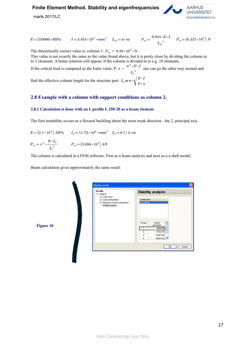
2.8 Example with a column with support conditions as column 2.

2.8.1 Calculation is done with an L profile L 250·20 as a beam element.

The first instability occurs as a flexural buckling about the most weak direction - the 2. principal axis.

=E ⎛⎝ ⋅2.1 105 ⎞⎠ MPa ≔I2 ⋅⋅11.72 106 mm4 ≔Ls ⋅⋅0.7 4 m

≔Pcr ⋅π 2 ――⋅E I2

Ls2

=Pcr⎛⎝ ⋅3.098 103 ⎞⎠ kN

The column is calculated in a FEM software. First as a beam analysis and next as a a shell model.

Beam calculation gives approximately the same result:

Figure 18

17


2.8.2 Calculation of the L profile L 250x20 as a shell model.

The first instability sits well with bar calculation. The next instabilities seems to vary somewhat from the beam calculation. This is because incomparable deformation shapes are compared. The beam calculationdoes not include deformations of the cross section itself, which is the model with shell elements takes in account.

Figure 20

18


3.0 FEM calculations of eigenfrequency.

3.1 Masse matrix.

Displacements acceleration expressed by shape functions.

＝u ((x)) ⋅φ ū ＝⋅u ((x)) '' ⋅φ ū'' ρ is the dead load of the beam in kg/m.

This will result in a force m·a in a random spot on the beam:

＝F ⋅⋅ρ φ ū'' as function for the beam.

These force summed up and converted to node forces,when the mass follows deformations or shape functions.

＝＝⌠⌡ d⋅φ F x ⋅⌠

⌡ d⋅⋅Tφ ρ φ x ū'' ⋅Ќm ū''

Masse matrix is defined as: ＝Ќm⌠⌡ d⋅⋅Tφ ρ φ x Tφ transposing due to calculations technics.

Masse matrix shows deformations of nodes according to shape functions.

＝Km ,2 3

⌠⎮⎮⌡

d

0

L

⋅⋅⋅-x⎛⎜⎝

+-⎛⎜⎝―x

L

⎞⎟⎠

2

⋅2 ―x

L1⎞⎟⎠ρ⎛⎜⎝

+⋅-2⎛⎜⎝―x

L

⎞⎟⎠

3

⋅3⎛⎜⎝―x

L

⎞⎟⎠

2 ⎞⎟⎠

x ＝Km ,2 3-――――

⋅⋅13 L2 ρ

420

＝Ќm ⋅――⋅ρ L

420

156 ⋅-22 L 54 ⋅13 L

⋅-22 L ⋅4 L2 ⋅-13 L ⋅-3 L

2

54 ⋅-13 L 156 ⋅22 L

⋅13 L ⋅-3 L2 ⋅22 L ⋅4 L2

⎡⎢⎢⎢⎢⎣

⎤⎥⎥⎥⎥⎦

19


3.2 Eigenfrequency problem formulated as a suspended spring.

Figure 21 The stiffness ＝k ⋅250 ――kg

s2

S is the static deformation from the mass.X is the dynamic deformation from the oscillation.

＝F1 ⋅k (( +s x)) ＝F2 ⋅M g ＝+F1 F2 ⋅M a

＝a ――d

d

2

t2x

＝⋅M ――d

d

2

t2x --⋅M g ⋅k s ⋅k x

＝-⋅M g ⋅k s 0 in equilibrium position we have static equilibrium.

＝+――d

d

2

t2x ⋅―

k

Mx 0 ＝+r2 ―

k

M0 ＝r +0 ⋅i

‾‾‾―k

M＝r -0 ⋅i

‾‾‾―k

M

＝x +⋅C1 cos⎛⎜⎝

⋅‾‾‾―k

Mt⎞⎟⎠

⋅C2 Sin⎛⎜⎝

⋅‾‾‾―k

Mt⎞⎟⎠

General solution.

＝x x0 for t=0 ＝x0 +⋅C1 cos⎛⎜⎝

⋅‾‾‾―k

Mt⎞⎟⎠

⋅C2 sin⎛⎜⎝

⋅‾‾‾―k

Mt⎞⎟⎠

boundary conditions:

＝C1 x0 ＝――d

dtx 0 for t=0

＝0 +⋅⋅-‾‾‾―k

Mx0 sin

⎛⎜⎝

⋅‾‾‾―k

Mt⎞⎟⎠

⋅⋅C2‾‾‾―k

Mcos

⎛⎜⎝

⋅‾‾‾―k

Mt⎞⎟⎠

≔C2 0

＝x ⋅x0 cos⎛⎜⎝

⋅‾‾‾―k

Mt⎞⎟⎠

Particular solution.

20


3.3 Beam formulation.

The result from the spring calculation is transformed to a beam problem, so the spring constant is the bending stiffness of the beam, and the dead load of the weight is the action on the beam.

Displacement for the beam with action as a single force: ＝x ⋅―1

c―――⋅P L3

⋅E I

c is a constant depending of where the forced is placed.

Hookes low: ＝P ⋅k x ＝＝k ―P

x⋅――

⋅E I

L3c

＝-⋅m g ⋅k (( +s x)) ⋅m a ＝+⋅m a ⋅k x 0 m is the mass matrix for a beam.

For a beam this will come from the stiffness matrix K. ＝+⋅Ќm ――d

d

2

t2x ((t)) ⋅Ќ x 0

＝＝＝x ((t)) ⋅x0 cos⎛⎜⎝

⋅‾‾‾―k

Mt⎞⎟⎠

⋅x0 cos (( ⋅ω t)) ⋅ū cos (( ⋅ω t)) u and is the boundary conditions. x0

The solution for x(t) is used in this term: ＝+⋅Ќm ――d

d

2

t2x ((t)) ⋅Ќ x 0

＝+⋅⋅⋅-Ќm ω2 ū cos (( ⋅ω t)) ⋅⋅Ќ ū cos (( ⋅ω t)) 0 ＝-⋅Ќ u ⋅⋅Ќm ω2 ū 0

＝⋅⎛⎝ -Ќ ⋅Ќm ω2 ⎞⎠ ū 0 With Cramers Rule: ＝‖‖ -Ќ ⋅Ќm ω2 ‖‖ 0

The eigenfrequency is: ＝n ⋅――1

⋅2 π

‾‾‾ω2

3.4 Example with IPE240. IPE240 L = L1+L2 = 10·m3.4.1 Teknisk Ståbi.

Figure 22≔K 15.4

＝ω ⋅――K

L2

‾‾‾‾――⋅E I

ρ≔L ⋅10000 mm

=E ⎛⎝ ⋅2.1 105 ⎞⎠ MPa ≔I ⋅⋅38.9 106 mm4 ≔ρ ⋅30.7 ――kg

m

≔n ⋅⋅――K

L2

‾‾‾‾――⋅E I

ρ――1

⋅2 π=n 12.643 ―

1

s Result is close to the EDB =n 12.643 ―1

s

calculation.

21


3.4 Example med IPE240.

＝L +L1 L2

Figure 23 ⇒

＝-⋅――⋅E I

L3

12 ⋅-6 L -12 ⋅-6 L

⋅-6 L ⋅4 L2 ⋅6 L ⋅2 L2

-12 ⋅6 L 12 ⋅6 L

⋅-6 L ⋅2 L2 ⋅6 L ⋅4 L2

⎡⎢⎢⎢⎢⎣

⎤⎥⎥⎥⎥⎦

⋅⋅ω2 ――⋅ρ L

420

156 ⋅-22 L 54 ⋅13 L

⋅-22 L ⋅4 L2 ⋅-13 L ⋅-3 L2

54 ⋅-13 L 156 ⋅22 L

⋅13 L ⋅-3 L2 ⋅22 L ⋅4 L2

⎡⎢⎢⎢⎢⎣

⎤⎥⎥⎥⎥⎦

000rC

⎡⎢⎢⎢⎢⎣

⎤⎥⎥⎥⎥⎦

＝ū

000rC

⎡⎢⎢⎢⎢⎣

⎤⎥⎥⎥⎥⎦

The determinant for this term can be expressed in equation: ⇒ ＝-⋅⋅E I ―4

L⋅⋅⋅λ ――

⋅ρ L

4204 L2 0

≔ω‾‾‾‾‾‾‾‾――――

⋅⋅420 E I

⋅L4 ρ=ω 105.716 ―

1

s≔n ――

ω

⋅2 π=n 16.825 ―

1

s

It is a poor result, which is to far from the theoretical correct result.

3.4.3 Example with 2 elements. ＝＝L1 L2 L ≔L ⋅5000 mm

＝＝L1 L2 L

＝＝E1 E2 E ＝ū

00uBrB0rC

⎡⎢⎢⎢⎢⎢⎢⎣

⎤⎥⎥⎥⎥⎥⎥⎦Figure 24 ＝＝I1 I2 I

＝Ќ ⋅――⋅E I

L3

12 ⋅-6 L -12 ⋅-6 L 0 0⋅-6 L ⋅4 L2 ⋅6 L ⋅2 L2 0 0

-12 ⋅6 L 24 0 -12 ⋅-6 L

⋅-6 L ⋅2 L2 0 ⋅8 L2 ⋅6 L ⋅2 L2

0 0 -12 ⋅6 L 12 ⋅6 L

0 0 ⋅-6 L ⋅2 L2 ⋅6 L ⋅4 L2

⎡⎢⎢⎢⎢⎢⎢⎣

⎤⎥⎥⎥⎥⎥⎥⎦

＝Ќmod ⋅――⋅E I

L3

24 0 ⋅-6 L

0 ⋅8 L2 ⋅2 L2

⋅-6 L ⋅2 L2 ⋅4 L

2

⎡⎢⎢⎣

⎤⎥⎥⎦

＝Ќ1m ⋅――⋅ρ L

420

156 ⋅-22 L 54 ⋅13 L 0 0

⋅-22 L ⋅4 L2 ⋅-13 L ⋅-3 L2 0 054 ⋅-13 L 156 ⋅22 L 0 0

⋅13 L ⋅-3 L2 ⋅22 L ⋅4 L2 0 00 0 0 0 0 00 0 0 0 0 0

⎡⎢⎢⎢⎢⎢⎢⎣

⎤⎥⎥⎥⎥⎥⎥⎦

＝Ќ2m ⋅――⋅ρ L

420

0 0 0 0 0 00 0 0 0 0 00 0 156 ⋅-22 L 54 ⋅13 L

0 0 ⋅-22 L ⋅4 L2 ⋅-13 L ⋅-3 L2

0 0 54 ⋅-13 L 156 ⋅22 L

0 0 ⋅13 L ⋅-3 L2 ⋅22 L ⋅4 L2

⎡⎢⎢⎢⎢⎢⎢⎣

⎤⎥⎥⎥⎥⎥⎥⎦

22


＝Ќm +Ќ1m Ќ2m

＝Ќm ⋅――⋅L ρ

420

156 ⋅-22 L 54 ⋅13 L 0 0⋅-22 L ⋅4 L2 ⋅-13 L ⋅-3 L2 0 0

54 ⋅-13 L 312 0 54 ⋅13 L

⋅13 L ⋅-3 L2 0 ⋅8 L2 ⋅-13 L ⋅-3 L2

0 0 54 ⋅-13 L 156 ⋅22 L

0 0 ⋅13 L ⋅-3 L2 ⋅22 L ⋅4 L2

⎡⎢⎢⎢⎢⎢⎢⎣

⎤⎥⎥⎥⎥⎥⎥⎦

＝Ќm_mod ⋅――⋅L ρ

420

312 0 ⋅13 L

0 ⋅8 L2 ⋅-3 L2

⋅13 L ⋅-3 L2 ⋅4 L2

⎡⎢⎢⎣

⎤⎥⎥⎦

=I ⎛⎝ ⋅3.89 107 ⎞⎠ mm4 =E ⎛⎝ ⋅2.1 105 ⎞⎠ MPa =L 5 m =ρ 30.7 ――kg

m

is 5700·ω2 ―1

s2＝

‖‖‖‖‖‖‖‖‖

-

⋅――24

L3⋅E I 0 ⋅-6 ⋅E ――

I

L2

0 ⋅―8

L⋅E I ⋅―

2

L⋅E I

⋅-6 ⋅E ――I

L2

⋅―2

L⋅E I ⋅―

4

L⋅E I

⎡⎢⎢⎢⎢⎢⎢⎢⎣

⎤⎥⎥⎥⎥⎥⎥⎥⎦

⋅ω2

―――⋅⋅26 L ρ

350 ――――

⋅⋅13 L2 ρ

420

0 ―――⋅⋅2 L3 ρ

105-――

⋅L3 ρ

140

――――⋅⋅13 L

2ρ

420-――

⋅L3ρ

140――

⋅L3ρ

105

⎡⎢⎢⎢⎢⎢⎢⎢⎣

⎤⎥⎥⎥⎥⎥⎥⎥⎦

‖‖‖‖‖‖‖‖‖

0

≔ω‾‾‾‾‾‾‾‾‾‾

⋅⋅5.7 103 ―1

s2=ω 75.498 ―

1

s=――

ω

⋅2 π12.016 ―

1

s

3.4.4 EDB calculation with Strusoft, FEM-Design.

FEM_Design with 2 elements: Result 12.14 is acceptable comparing to the result above ( ).⋅12.02 ―1

s

Figure 25

23


FEM-Design with 20 elements: Result 12.64

Figure 26

24


4.0 Exercises.

4.1) Forces and reactios.

4.11) Find 2 values in the general stifness matrix for one horizontal beam with vertical load.Find and .K34 K21

4.12) FEM calculations of reactions, forces and deformations.Make a FEM calculation for the beam in Figure 27a. The beams must be divided into 2 elements. Calculations for reactions, forces and displacement as functions.

4.13) FEM calculations of reactions and forces.Make a FEM calculation for the beam in Figure 27b and controls result in FEM-Design with your own numerical. The beams must be divided into 2 elements. Calculations for reactions and forces.

4.14) FEM calculation i FEM software.Find a symbolic solution for the reactions in the shown sloped beam in Figure 28.Find a symbolic solution for the bending moment in C and controls result in FEM-Design with your own numerical.

4.2) Critical load.4.21) Find 2 values in the general geometric stifness matrix for one horizontal beam with vertical load.Find and Ќσ34 Ќσ12

4.22) Manual FEM calculation for the critical load.Find the critical load for column 2 by the means of 2 element in Figure 14-17.

4.23) FEM calculation for the critical load with FEM-software.Find the critical load for column 2 by the means of a FEM-software. (FEM-Design from Strusoft).

4.3) Effective column length.4.31) FEM calculation of welded section.Find the effective column length for det shown HEA200 profile below with plates t = 10·mm welded onboth sides in Figure 29.

First as a beam calculation and second as a profile modeled with shell elements. L = 3·m.

FEM-Design is recommended.

Figure 27a Figure 27b

25


Figure 28

If the calculated critical load is equalizid with the Euler force

the effective ＝⋅P λ ―――⋅⋅π2 E I

Ls2

columnlength can be determined by isolation the column length for

a structure part: ＝Ls ⋅π‾‾‾‾‾――⋅E I

⋅P λ

Figure 29

4.32) See Figure 30 below for a frame.a) Find the effective column length for the column AB, when support C is simple. Column and beam HEB160.b) Find the effective column length for the column AB, when support C is simple and roller supported. Column and beam HEB160.c) Find the effective column length for the column AB from b), when beam BC is chanced from HEB160 to HEB240

Figure 30

26


4.4) eigenfrequencies.4.41) eigenfrequencies. Find the 2 first eigenfrequencies for the structure column 1 in Figure 14-17. Column 1 must be rotated 90 deg. so it will appear as horizontal beam. The beam must be calculated manually.

4.42)Find the 2 first eigenfrequencies for the structure from exercise 4.32, performed with FEM software.

4.5) 2-hinged frame and 1-hinged frame.4.51) Reactions.Find by manual calculations an expression for the horizontal reactions in the frame as shown below in figure 32:Determine how the ratio I/A affects the result. Beam and columns are assumed to have the cross section in this exercise.

figure 32:

27


4.52) Effective column lengths.Find by manual calculations the effective column length for column 1 and column 2 in Figure 14-17, when both columns and the beam between is a 1-hinged frame med stiff corners. Columns KKR 120·120·6.3and the beam KKR 120·200·6.3. Calculations must be confirmed with use of a FEM software.Calculation is performed as a sway structure and as non sway structure in the FEM software.Statically system is shown in figure 31.

4.53) Effective column lengths.Find the effective column length for column 1 and column 2, when both columns and the beam between is a 1-hinged frame med stiff corners. Column 1 is KKR 120·120·6.3, column 2 is KKR 200·120·6.3 and thebeam KKR 120·200·6.3. Calculation is performed as a sway structure and as non sway structure in the FEM software. Statically system is shown in figure 31.

4.54) eigenfrequencies.Find the 4 first eigenfrequencies for the structure in 4.53) as a sway structure.

Figure 31

References

[1] Elementmetoden for bjælkekonstruktioner af Lars Damkilde Ålborg Universitet Esbjerg.

[2] Analysis and Design of Elastic Beams bye Walter D. Pilkey.

[3] Grundlæggende elementmetode for Bjælker og Rammer af Sven Krabbenhoft, Aalborg Universitet Esbjerg.

[4] Concepts and applications of finite element analysis. Robert D. Cook. 4.th edition.

28

finite element method. stability and eigenfrequenciesstaff.iha.dk/lc/fem/fem_noter/civil/bk101.2...

Documents