1

Finite Element Course

ANSYS Mechanical Tutorial

Tutorial 4 – Plate With a Hole

Problem Specification

Consider the classic example of a circular hole in a rectangular plate of constant thickness. The plate is A514 steel with a modulus of elasticity of 29e6 psi and a Poisson ratio of 0.3. The thickness of the plate is .2 in., the diameter of the hole is .5 in., the length of the plate is 10 in. and the width of the plate 5 in., as the figure below indicates.

Step 1: Start-up & preliminary set-up

Pre-Analysis and Start-Up

Analytical vs. Numerical Approaches

We can either assume the geometry as an infinite plate and solve the problem analytically, or approximate the geometry as a collection of "finite elements", and solve the problem numerically. The following flow chart compares the two approaches.

2

Let's first review the analytical results for the infinite plate. We'll then use these results to check the numerical solution from ANSYS.

3

Analytical Results

Displacement

Let's estimate the expected displacement of the right edge relative to the center of the hole. We can get a reasonable estimate by neglecting the hole and approximating the entire plate as being in uniaxial tension. Dividing the applied tensile stress by the Young's modulus gives the uniform strain in the x direction.

Multiplying this by the half-width (5 in) gives the expected displacement of the right edge as ~ 0.1724 in. We'll check this against ANSYS.

Sigma-r

Let's consider the expected trends for Sigma-r, the radial stress, in the vicinity of the hole and far from the hole. The analytical solution for Sigma-r in an infinite plate is:

where a is the hole radius and Sigma-o is the applied uniform stress (denoted P in the problem specification). At the hole (r=a), this reduces to

This result can be understood by looking at a vanishingly small element at the hole as shown schematically below.

4

We see that Sigma-r at the hole is the normal stress at the hole. Since the hole is a free surface, this has to be zero.

For r>>a,

Far from the hole, Sigma-r is a function of theta only. At theta = 0, Sigma-r ~ Sigma-o. This makes sense since r is aligned with x when theta = 0. At theta = 90 deg., Sigma-r ~ 0 which also makes sense since r is now aligned with y. We'll check these trends in the ANSYS results.

Sigma-theta

Let's next consider the expected trends for Sigma-theta, the circumferential stress, in the vicinity of the hole and far from the hole. The analytical solution for Sigma-theta in an infinite plate is:

At r = a, this reduces to

At theta = 90 deg., Sigma-theta = 3*Sigma-o for an infinite plate. This leads to a stress concentration factor of 3 for an infinite plate.

For r>>a,

5

At theta = 0 and theta = 90 deg., we get

Far from the hole, Sigma-theta is a function of theta only but its variation is the opposite of Sigma-r (which is not surprising since r and theta are orthogonal coordinates; when r is aligned with x, theta is aligned with y and vice-versa). As one goes around the hole from theta = 0 to theta = 90 deg., Sigma-theta increases from 0 to Sigma-o. More trends to check in the ANSYS results!

Tau-r-theta

The analytical solution for the shear stress Tau-r-theta in an infinite plate is:

At r=a,

By looking at a vanishingly small element at the hole , we see that Tau-r-theta is the shear stress on a stress surface, so it has to be zero.

6

For r>>a,

We can deduce that, far from the hole, Tau-r-theta = 0 both at theta = 0 and theta = 90 deg. Even more trends to check in ANSYS!

Sigma-x

First, let's begin by finding the average stress, the nominal area stress, and the maximum stress with a concentration factor.

The concentration factor for an infinite plate with a hole is K = 3. The maximum stress for an infinite plate with a hole is

Although there is no analytical solution for a finite plate with a hole, there is empirical data available to find a concentration factor. Using a Concentration Factor Chart (Cornell 3250 Students: See Figure 4.22 on page 158 in Deformable Bodies and Their Material Behavior), we find that d/w = 1 and thus K ~ 2:73 Now we can find the maximum stress using the nominal stress and the concentration factor

Open ANSYS Workbench

Now that we have the pre-calculations, we are ready to do a simulation in ANSYS Workbench! Open ANSYS Workbench by going to Start > ANSYS > Workbench. This will open the start up screen as seen below

7

To begin, we need to tell ANSYS what kind of simulation we are doing. If you look to the left of the start up window, you will see the Toolbox Window. Take a look through the different selections. The plate with a hole is a static structural simulation. Load the static structural tool box by dragging and dropping it into the Project Schematic.

Name the Project "Plate with a Hole" by double clicking the text Static Structural and

typing in Plate with a Hole.

8

Material Selection

Now we need to specify what type of material we are working with. Double click Engineering Data and it will take you to the Engineering Data Menus.

If you look under the Outline of Schematic A2: Engineering Data Window, you will see that the default material is Structural Steel. The Problem Specification specifies the material's Modulus of Elasticity and Poisson's ratio. To add a new material, click in an empty box labeled Click here to add a new material and give it a name. We will call our

material Cornellium.

9

On the left hand side of the screen in the Toolbox window, expandLinear Elastic and double click Isotropic Elasticity to specify the Elastic Modulus and Poisson's Ratio.

In the Properties of Outline Row 4: Cornellium window, Set the Elastic Modulus units

to psi, set the magnitude as 29e6, and set the Poisson's Ratio to .3.

Close the materials window by selecting Return to Project.

Now that the material has been specified, we are ready to make the geometry in ANSYS.

Geometry For users of ANSYS 15.0, please check this link for procedures for turning on the Auto Constraint feature before creating sketches in DesignModeler.

10

Analysis Type

First, right click and click Properties to bring up the geometry properties menu. The default analysis type of ANSYS is 3D, but we are doing a 2 dimensional problem. Change the Analysis Type from 3D to 2D .

Next double click . This will bring up the Design Modeler. It will prompt you to pick the standard units. Since all of the units in the problem specification were given in English units, we want to choose inch . When the Inch radio button is selected, press OK

Draw the Geometry

To begin sketching, we need to look at a plane to sketch on. Click on the Z-axis of the compass in the bottom right hand corner of the screen to look at the x-y plane.

11

Now, look to the sketching toolboxes window and click the sketching tab; this will bring up the sketching menu.

Before we sketch the geometry, let's note something about the problem specification. The geometry itself has two planes of symmetry: it is symmetric about the x-plane and y-plane. This means we can model 1/4 of the geometry, and use symmetry constraints to represent the full geometry in ANSYS. If me model a quarter of the geometry, we can make the problem less complex and save some computational time.

Okay! Let's start sketching. First, click in the sketching tool bar. This tool defines a rectangle by two points. Place the first point at the origin (Watch for the P- symbol which shows you are placing the point at the origin point), and the other point somewhere in the first quadrant.

12

Now, click . This tool allows to define a circle by clicking once to define its center point, then click a distance away from the center point to define a radius. Define the circle so its center point is at the origin, define the radius by clicking somewhere inside the rectangle.

We almost have a geometry, but we first need to get rid of the superfluous lines. In the sketching toolboxes window, click Modify > Trim .

13

Now, trim the segments that are 1. outside of the 1st quadrant, and 2. between the circle and the origin. You should end up with something similar to the following figure.

Dimensions

Now, we have to dimension the drawing to the problem specification. (Remember! We are only drawing 1/4 of the geometry, so we need to take this into account when dimensioning the figure in ANSYS). In the sketching toolboxes window, click Dimensions > General

14

This tool will allow you to define dimensions that you can specify. We need to specify the rectangle's length and width, and the circle's radius. Use the tool to define the height of the rectangle (the right edge of the geometry), the length of the rectangle (the top edge of the rectangle), and the radius of the circle. You should end up with the following window.

15

To specify the dimensions, look to the Details View Window.

Change the H (for horizontal) dimension to 5 inches, the V (for vertical) dimension to 2.5 inches, and the R (for radius) dimension to .25 inches. Now we have the geometry specified in the problem statement sketched in ANSYS.

16

Create a Surface from the Sketch

Next, we need to tell ANSYS what type of geometry we are modeling. For this problem, we will create a surface and give it a thickness. In the menu bar, select Concept > Surfaces from Sketches . To select the sketch, look to the outline window, and expand XY plane > Sketch 1 .

In the details window pane, select Base Objects > Apply . Now, we need to specify a thickness. Specify the thickness as .1 inches, as from the problem statement. Now in the

menu toolbar, click This should generate the geometry.

Close the Deign Modeler (don't worry, the geometry will be saved in the project automatically). Now we are ready to mesh the geometry.

17

Mesh

Face Sizing

Now, double click Model in the project outline to bring up the Mechanical window.

Go to Units > U.S. Customary (in. lbm, lbf, F, s, V, A) to make sure the proper units are selected.

To begin the Mesh process, click Mesh in the outline window. This will bring up the Mesh Menu bar in the Menu bar.

We want to control the size of the elements in the mesh for this problem; to accomplish this, click Mesh Control > Sizing. We now need to pick the geometry we are going to

mesh. Make sure the Face Selection Filter is selected then click the face of the

18

geometry to select it. In theDetails window click Geometry > Apply. Now, we can set some of the details of our mesh. Select Element Size > Default, this will allow you to change the size of the element. Choose the size of the elements to be.05 in.

Turn off the Advanced Size Function in the details window of "Mesh". If we leave the Advanced Size Function on, ANSYS will override the face sizing we applied.

Edge Refinement

Now, we want to refine the mesh by the hole, where we expect a stress concentration. Go to Mesh Control > Refinement. This will open the Refinement menu if the details view window. To select the hole as the geometry for refinement, make sure the edge

19

select tool is selected from the menu toolbar. Now, select the hole's edge then click Geometry > Apply.

In the details window, change the Refinement parameter from 1 to 3, this will give us the finest mesh at the hole which will improve accuracy of the simulation.

Now that we have our mesh setup, click Mesh > Generate Mesh. This will create the

mesh to our specifications. Click to display it. It should look something like this:

Now that the mesh has been created, we are ready to specify the boundary conditions of the problem.

20

Physics Setup

Specify Material

First, we will tell ANSYS which material we are using for the simulation. Expand Geometry, and click Surface Body in the Outline window. In theDetails window, select Material > Assignment > Cornellium. The material has now been specified.

Symmetry Conditions

First, let's start by declaring the symmetry conditions in the problem. Right click Model > Insert > Symmetry.

21

This will create a symmetry folder in the outline tree Now, right click Symmetry > Insert > Symmetry Region. Make sure the Edge Select Tool is highlighted and select the left edge above the hole.

22

Now look to the Details View window and select Geometry > Apply. This should create a red line with a tag on the model. Ensure that underSymmetry Normal the x-axis is selected. Repeat this process to create a symmetry region for the bottom edge to the right of the hole, but this time making sure that the Symmetry Normal parameter is the y-axis.

Forces

Now, we can specify the forces on the body. Click Static Structural in the outline tree. This will bring up the Physics Sub-Menu bar in the Menu Bar.

23

Click Loads > Pressure to specify a traction. Select the right edge of the geometry and apply it in the details view window. The pressure's magnitude from the problem

specification is -1e6 psi (pressure in ANSYS defaults to compression, and we need tension, hence the negative sign). Now that the forces have been set, we need to set up the solution before we solve.

Numerical Solution

Now we are ready to choose what kind of results we would like to see.

Deformation

To add deformation to the solution, first click Solution to add the solution sub menu to menu bar

24

Now in the solution sub menu click Deformation > Total to add the total deformation to the solution. It should appear in the outline tree.

Normal Stresses

Sigma_xx

To add the normal stress in the x-direction, in the solution sub menu go to Stress > Normal. In the details view window ensure that theOrientation is set to X Axis. Let's

rename the stress to Stress_xx by right clicking the stress, and going to rename.

Sigma_r

To add the polar stresses, we need to first define a polar coordinate system. In the outline tree, right click Coordinate System > Insert > Coordinate System.

This will create a new Cartesian Coordinate System. To make the new coordinate system a polar one, look to the details view and change theType Parameter from Cartesian to Cylindrical. To define the origin, change the Define By parameter from Geometry to Global Coordinate System. Put the origin coincident with the global coordinate systems origin (x = 0, y = 0). Now that the polar coordinates have been created, lets rename the coordinate system to make it more distinguishable. Right click on the coordinate system

you just created, and go to Rename. For simplicity sake, let's just name it Polar

Coordinates.

25

Now, we can define the radial stress using the new coordinate system. Click Solution > Stress > Normal. This will create "Normal Stress 2", and list its parameters in the details view. We want to change the coordinate system to the polar one we just created; so in the details view window, change the Coordinate System parameter from "Global Coordinate System" to "Polar Coordinates". Ensure that the orientation is set to the x-axis, as defined by our polar coordinate system. Now the stress is ready. Let's rename it

to Sigma_r and keep going.

Sigma_theta

Now let's add the theta stress. This is too a normal stress, so create a new normal stress as you did for Sigma_xx and Sigma_r. Now, change the coordinate system to Polar Coordinates, as you did for Sigma-r. Next, change the Orientation to the Y axis. The Y

axis should be in the theta direction by default. Rename the stress to Sigma_theta.

26

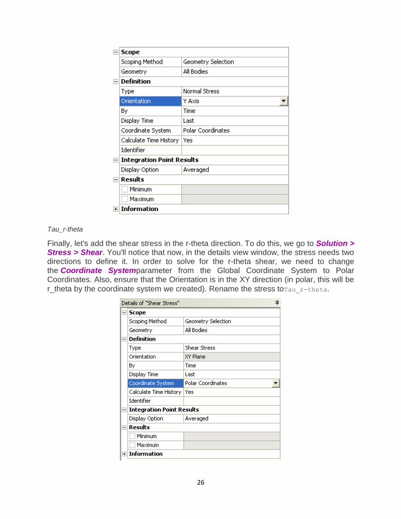
Tau_r-theta

Finally, let's add the shear stress in the r-theta direction. To do this, we go to Solution > Stress > Shear. You'll notice that now, in the details view window, the stress needs two directions to define it. In order to solve for the r-theta shear, we need to change the Coordinate Systemparameter from the Global Coordinate System to Polar Coordinates. Also, ensure that the Orientation is in the XY direction (in polar, this will be

r_theta by the coordinate system we created). Rename the stress toTau_r-theta.

27

This is what your outline tree should look like at this point:

Solve!

To solve for the stresses and deformation, we now hit the solve button.

Keep going! Almost done!

Numerical Results

Displacement

Okay! Now let's look at the numerical solution to the boundary value problem as calculated by ANSYS. Let's start by examining how the plate deformed under the load. Before you start, make sure the software is working in the same units you are by looking to the menu bar and selecting Units > US Customary (in, lbm, lbf, F, s, V, A). Also,

select the pan tool by clicking the pan button from the top bar. This will allow you to zoom by scrolling the mouse wheel, and move the image by left-clicking and dragging.

28

Now, look at the Outline window, and select Solution > Total Deformation. First, we will look at just the deformation of the plate, without contours. To do this, select the Contours

button, , and select Solid Fill.

There are a few things we can determine from this picture. Let's use our intuition and the work we did in the pre-analysis to compare to the result ANSYS gives us. First, let's look at the bottom and left edges of the plate. We can see that the deformation on these edges is parallel to the sides, which agrees with the symmetry boundary condition. The top edge of the plate has deformed downwards, which is due to the effects of Poisson's ratio. The right edge has moved to the right, which is consistent with the expected behavior, due to the plate being in tension. So we can deduce the following boundary conditions from looking at the deformation.

Animate the deformation by pressing Play in the Animation tool bar along the bottom of the screen. This linearly interpolates between the initial and final deformed state.

29

To get back the color contours of deformation values, select the Contours button and choose Contour Bands. The colored section refers to the magnitude of the deformation (in inches) while the black outline is the undeformed geometry superimposed over the deformed model. The more red a section is, the more it has deformed while the more blue a section is, the less it has deformed. Notice that far from the hole, the deformation is linearly varying, similar to a bar in tension. Now let's look at the value of the largest deformation. Looking at the top of the color bar, we see that the largest deformation is 0.176 inches. From our pre-analysis, we estimated that the deformation was ~ 0.17 inches - a 2% difference. This is one check on our ANSYS result.

Save Image to a File

You can save the image to a file using the Image to File option shown below.

Sometimes, you get an error saying "The display settings are Windows Aero and image capture might not work." In that case, you can use the Windows 7 snipping tool which can be accessed from the Start > Programs menu as shown below.

30

Draw a rectangle around the screen area that you want to capture and save to an image file.

Sigma-r

Now let's look at the radial stresses in the plate. Look to the outline window and click Solution > Sigma-r. This will display the radial stresses.

Does this match what we expect? First, let's examine the hole at r = a. From our pre-calculations, we found that the stress at the hole in the radial direction should be 0. Zooming in with the middle mouse wheel and using our probe tool, we find that the stress in this area ranges from -450 to 450 psi. Although the simulation does not approach exactly zero, keep in mind that 450 psi is less than 1% of the average stress, so it can be thought of as approximately zero. Also, we expect this value to get closer to zero as we refine the mesh.

31

In order to zoom out and view the whole solution, select the zoom to fit button from the toolbar.

Now, let's first look at the case when r >> a. As we found in the pre-calculations, when r >> a, the radial stress is a function of the angle theta only. This matches the behavior

seen in the simulation. From our Pre-Calculations, we also found that . Using the probe tool, we find that indeed at this location, the stress is equal to 1e6 psi, which is the value we calculated in our Pre-Analysis. Also from our Pre-Analysis, we

found that when . Checking the simulation with our trusty probe tool, we find that the ANSYS simulation matches up quite nicely with our calculation.

Sigma-Theta

Now, let's compare the simulation to our pre-calculations for the theta stress. Look to the Outline window, then click Solution > Sigma-theta

First, let's compare the case when r = a. From the pre-analysis, we found that the stress at the hole acts as a function of theta. Specifically:

From this equation, we find that at zero degrees, we expect the stress to be -1e6 psi at zero degrees and at 90 degrees, we expect the stress to be 3e6 psi. Zoom in close to the hole to view the stresses there. From the simulation we find that the stress at 0 degrees

32

is -1.0285e6 psi (a 3% deviation), and the stress at 90 degrees is 3.0323e6 psi (a 1 % deviation). The deviations are due to the infinite plate assumption in the theory.

Now, let's look at the case when r >> a. From our pre-calculations, we found that the theta stress is a function of theta only. This behavior is represented in the simulation.

Also, for r >> a and the stress is equal to . Using the probe tool and hovering over this area, we see that the stress is indeed equal

to Sigma-o. However, looking at the area when , we find that the stress from the simulation is between 1000 psi and 2000 psi. Although this seems large compared to zero, one must keep in mind that the stress at this location is 1% of the average stress. We expect that the stress here will get closer to zero on refining the mesh since the numerical error becomes smaller.

Tau-r-theta

Now let's look at how the simulation match our predictions for the shear stress. Look to the Outline window, then click Solution > Tau-r-theta

In our pre-analysis, we determined that at r = a the shear stress should be 0 psi. Using our probe tool, we find that the stress ranges between -5 and -500 psi at the hole. Because 500 psi is .05% of the average stress, we can say this result does represent what we expect to happen very well.

In our pre-calculations, we determined that far from the hole the shear stress should be a function of theta only. This can be shown by using the probe tool a hovering over a radial line from the hole. The colors (representing higher and lower stresses) only change only as the angle changes, but not as the move away from the hole. We also found that far from the hole at the stress is zero

33

Using the probe tool, we can see that this is indeed the case for the simulation as well.

Sigma-x

Now lets examine the stress in the x-direction. Look to the Outline window, then click Solution > Sigma-x

From this, you can see that most of the plate is in constant stress, and there is a stress concentration around the hole. The more red areas correspond to a high, tensile (positive) stress and the bluer areas correspond to areas of compressive (negative) stress. Let's use the probe tool to compare the ANSYS simulation to what we expected from calculation. In the menu bar, click the Probe button; this will display the Sigma-x values

at the cursor location as you hover over the plate.

Start by hovering over the area far from the hole. The stress is about 1e6 psi, which is the value we would expect for a plate in uniaxial tension. If you click the max tag (located adjacent to the probe tool in the menu bar), it will locate and display the maximum stress, which is shown as 3.0335e6 psi. This is about a 0.0055% difference from the calculation we did in the Pre-Analysis, which is a negligible difference.

Sigma-x along an edge

The stress along the left edge of the model can be found very easily. Remember, this is a quarter model, hence the left edge of the model is actually the center line of the full plate. In the Outline tree, insert Construction Geometry as shown in the following figure:

34

Right click on construction geometry and insert a path and rename it "left edge".

35

Enter the following start and end coordinates:

You should see a gray path displayed on the left edge of the model.

Add a normal stress object under Solution in the tree: Stress > Normal. Change the scoping method to Path and select left edge for Path.

36

Click on Solve to generate the result. ANSYS Mechanical will plot the stress along the left edge and the data is tabulated.

You can export the tabular data in Excel or text format by right-clicking on it.

37

Verification & Validation

Now that we have our results, it is important that we check to see that our computational simulation is accurate. One possible way of accomplishing this task is comparing to the pre-calculations, as we did in the results section. Another way to check our results is by refining the mesh further. The smaller the elements in the mesh, the more accurate our simulation will be, but the simulation will take longer. To refine the mesh, look to the outline tree and click Mesh > Face Sizing Change the element sizing to 0.025 in (half the size of the mesh we originally tried). The new mesh looks like this . It has twice as many elements as the original.

Now hit solve. Compare the values for your stresses with those we found for the original mesh. Are the very different? Or do they seem to approach a limit? If the latter, the mesh is refined enough and if you modeled the problem correctly, you are done! Below are the values from our original mesh, followed by the values for our refined mesh.

Maximum Sigma_xx Maximum Deformation

Theory Values 3.0033 x 10^6 psi 0.1724

Original Mesh 3.0336 x 10^6 psi 0.1761

Refined Mesh 3.0360 x 10^6 psi 0.1759

As one can see from the table above the results do not change greatly as the mesh is refined. This means we don't need to refine the mesh further.

We're Done!