finite element computer program analyze … · most widely used membrane element: the...

N

Ix U

I

FINITE ELEMENT COMPUTER PROGRAM TO ANALYZE CRACKED ORTHOTROPIC SHEETS

C. S. Chn, J. M , Anderson, W. J. Batdorj and J. A. Aberson

Prepared by LOCKHEED-GEORGIA CQMPANY Marietta, Ga. 30063

for Langley Research Center

NATIONAL AERONAUTICS AND SPACE ADMINISTRATION WASHINGTON, D. C. JULY 1976

https://ntrs.nasa.gov/search.jsp?R=19760020511 2018-09-09T08:46:29+00:00Z

1. Repon No. . .

2. Government Accession No.

NASA CR-2698 4. Title and Subtitle

FINITE ELEMENT COMPUTER PROGRAM TO ANALYZE - CRACKED ORTHOTROPIC SHEETS - ~~~~

7. Author(s)

C. S. Chu; J. M. Anderson; W. J. Batdorf; and J. A. Aberson

. .

- . .. ~~ ~

National Aeronautics and Space Administration Washington D.C. 20546

3. Recipient's Catalog No.

5. Report Date JULY 1976

6. Performing Organization Code

8. Performing Organization Report No.

10. Work Unit No.

11. Contract or Grant No.

NAS1-13605 13. Type of Report and Period Covered

Contractor Report 14. Sponsoring Agency Code

743-01-11-02

I I - . .~ . .. ." ." .- ." ~

15. Supplementary Notes

FINAL REPORT Langley Technical Monitor: C. C. Poe, Jr. " - . . ~ " . -~ -~ . - . . - , . . ~. .-

16. Abstract

A finite-element computer program was developed to analyze a two-dimensional orthotropic

sheet with through-the-thickness cracks and temperature gradient, The program includes

special crack-tip elements that account for the singular stress fields associated with

crack opening (Mode I) and crack sliding (Mode 11) displacements at the crack tip.. The

program also includes a linear spring element and a constant-strain, triangular element.

A number of problems for which closed-form solutions exist were analyzed to demonstrate

the capabilities of the program.

". - _ ~ _ ~" ~

117. Key Words (Suggested by Author(s)) , - - - - L _ ~ _ ~

I orthotropic; composite materials; finite element;

crack; crack-tip element; stress intensity factor;

18. Distribution Statement

Unclassified-Unlimited

I thermal; computer program Subject Category 39

19. Security Clasrif. (of this report) 20. Security Classif. (of this page) -~

1 21. No;;f Pages

22. Price'

Unclassified Unclassified $4.75

For sale by the National Technical Information Service, Springfield, Virginia 22161

I

.....

TABLE OF CONTENTS

Page

LIST OF FIGURES . . . . . . . . . . . . . . . . . . . . . . . . . . . . . . . . . . . v

LIST OF TABLES . . . . . . . . . . . . . . . . . . . . . . . . . . . . . . . . . . . . vi i

SUMMARY . . . . . . . . . . . . . . . . . . . . . . . . . . . . . . . . . . . . . . . 1

INTRODUCTION . . . . . . . . . . . . . . . . . . . . . . . . . . . . . . . . . . . 2

SYMBOLS . . . . . . . . . . . . . . . . . . . . . . . . . . . . . . . . . . . . . . 3

BASIC EQUATIONS FOR FINITE ELEMENT PROGRAM . . . . . . . . . . . . . . . . 6

Matrix Equations for Stiffness Method . . . . . . . . . . . . . . . . . . . . . . . 6

Transformation of Elastic and Thermal Coefficients . . . . . . . . . . . . . . . . 7 TWO-DIMENSIONAL ELASTIC SOLUTIONS FOR CRACK-TIP STRESSES AND DISPLACEMENTS . . . . . . . . . . . . . . . . . . . . . . . . . . . . . . . . . . . 9

Distinct Roots 01. f g2) . . . . . . . . . . . . . . . . . . . . . . . . . . . . . . IO Repeated Roots (p. = I 2 = p) . . . . . . . . . . . . . . . . . . . . . . . . . . . 13

FORMULATION OF CRACKED ELEMENT STIFFNESS MATRICES . . . . . . . . . . . x) Anisotropic Case . . . . . . . . . . . . . . . . . . . . . . . . . . . . . . . . . 21

isotropic Case . . . . . . . . . . . . . . . . . . . . . . . . . . . . . . . . . . . 23

STRESS-INTENSITY FACTORS AND STRAIN-ENERGY RELEASE RATES . . . . . . . . 26

Stress- Intensity Factors . . . . . . . . . . . . . . . . . . . . . . . . . . . . . . 26

Strain-Energy Release Rates . . . . . . . . . . . . . . . . . . . . . . . . . . . . 26

BRIEF DESCRIPTION OF CRACKED ELEMENT COMPUTER PROGRAM . . . . . . . . 28

SAMPLE PROBLEMS . . . . . . . . . . . . . . . . . . . . . . . . . . . . . . . . . . 33

Anisotropic Case . . . . . . . . . . . . . . . . . . . . . . . . . . . . . . . . . 33

Center-Cracked and Double-Edge-Cracked Orthotropic Tension Plates . . . 33

Longitudinally Cracked Orthotropic Strip . . . . . . . . . . . . . . . . . . 39

45-Degree Cracked Finite Orthotropic Plate . . . . . . . . . . . . . . . . 39

... I l l

..

.

I

TABLE OF CONTENTS (Continued)

Page

Isotropic Case . . . . . . . . . . . . . . . . . . . . . . . . . . . . . . . . . . . 42

Cracked Tension Plates . . . . . . . . . . . . . . . . . . . . . . . . . . . . 42

Bi-Material Cracked Plate . . . . . . . . . . . . . . . . . . . . . . . . . . 42

Stiffened Plate . . . . . . . . . . . . . . . . . . . . . . . . . . . . . . . . 44

Thermal Stress-Intensity Problem . . . . . . . . . . . . . . . . . . . . . . . 44 APPENDIX . ELEMENT STIFFNESS MATRICES ..................... 49

REFERENC.ES. . . . . . . . . . . . . . . . . . . . . . . . . . . . . . . . . . . . . . 57

FIGURES . . . . . . . . . . . . . . . . . . . . . . . . . . . . . . . . . . . . . . . . 59

IV

LIST OF FIGURES

Figure

1

2

6

7 8

9 10

11

12

13

14

15

16

17

18

19

20

21

22

23 A1

A2

A3

Title Page . Triangular Element Material Axis .................... 59

Crack-Tip Neighborhood . . . . . . . . . . . . . . . . . . . . . . . . 59

Cracked Finite Elements . . . . . . . . . . . . . . . . . . . . . . . . 60 Segment Structure for Computer Program . . . . . . . . . . . . . . . . 61 Overall Logic Flow of Computer Program . . . . . . . . . . . . . . . . 62

Cracked Orthotropic Tension Plate Finite-Element Models . . . . . . . 64

Longitudinally Cracked Orthotropic Strip . . . . . . . . . . . . . . . 65

4.5' Cracked Finite Orthotropic Plate . . . . . . . . . . . . . . . . . . 67

45' Cracked Orthotropic Plate Finite-Element Model . . . . . . . . . . 68

and Center Cracked Tension Panels (a /w = 1/3) . . . . . . . . . . . . . 69

and Center Cracked Tension Panels (a/w = 1/3) . . . . . . . . . . . . . 70

Element . . . . . . . . . . . . . . . . . . . . . . . . . . . . . . . . . 71

Bi-Material Cracked Plate . . . . . . . . . . . . . . . . . . . . . . . 72

Bi-Material Plate Finite-Element Model . . . . . . . . . . . . . . . . 73 Stress in Bi-Material Cracked Plate . . . . . . . . . . . . . . . . . . . 74

Displacements of Cracked Faces in Bi-Material Plate . . . . . . . . . . 74

Effect of Riser on Stress Intensity in Plate. . . . . . . . . . . . . . . . 76 Geometry of the Thermal Stress Problem . . . . . . . . . . . . . . . . 77

Vector Representation for Thermal Problem . . . . . . . . . . . . . . . 77 Finite-Element Representation of Thermal Stress Problem . . . . . . . . 78

Axial Element . . . . . . . . . . . . . . . . . . . . . . . . . . . . . . 79

Triangular Element Membrane Displacements . . . . . . . . . . . . . . 79 Convention for Degrees of Freedom . . . . . . . . . . . . . . . . . . . 79

Center-Cracked and Double-Edge-Cracked Orthotropic Tension Plate . 63

Finite-Element Models for Longitudinally Cracked Orthotropic Strip. . 66

Symmetric Cracked Element Model for Single-Edge. Double.Edge.

Unsymrnetric Cracked Element Model for Single-Edge. Double.Edge.

Eccentric Crack (Isida's Problem) Model with Two 8-Node Cracked

Stiffened Plate . . . . . . . . . . . . . . . . . . . . . . . . . . . . . 75

V

Figure

A4

A5

A6

A7

LIST OF FIGURES . Continued

Tit le . Page

ShearPin ................................ 80

Direction Vectors for Fast-ner Element . . . . . . . . . . . . . . . . . 80

Spring System to Simulate Shear Pin . . . . . . . . . . . . . . . . . . 81

Local Coordinate System for Ten-Node Cracked Element . . . . . . . . 81

vi

LIST OF TABLES

Table T i t le Page . . I Elastic Coefficients Relating Energy Rates to Stress-Intensity Factors . . . . 27

I I Function of Subroutines . . . . . . . . . . . . . . . . . . . . . . . . . . . 30 111 Complex Roots of Characteristic Equation . . . . . . . . . . . . . . . . . . 34

IV

V

V I

VI1

Vl l l

IX

X

Stress-Intensity Factors of Center-Cracked Plates (a = 15.24 mm. a/w = 0.4) . . . . . . . . . . . . . . . . . . . . . . . . . . . . . . . . . 35 Stress-Intensity Factors of Center-Cracked Plates (a = 22.86 mm. a/w = 0.6) . . . . . . . . . . . . . . . . . . . . . . . . . . . . . . . . . 36

Stress-Intensity Factors of Double-Edge-Cracked Plates (a = 15.24 mm. a/w = 0.4) . . . . . . . . . . . . . . . . . . . . . . . . . . . . . . . . . 37 Differences from Snyder and Cruse's Results . . . . . . . . . . . . . . . . 35

Laminate Stiffness Matrices (Scotchply 1002) . . . . . . . . . . . . . . . . 4'0

Summary of Results for a Longitudinally Cracked Orthotropic Strip . . . . . 41

Summary of Typical Results for Isotropic Tension Plate . . . . . . . . . . . 43

v i i

FINITE ELEMENT COMPUTER PROGRAM TO ANALYZE CRACKED ORTHOTROPIC SHEETS

Chorng-Shin Chu J. M. Anderson* W. J. Batdorf J. A. Aberson**

SUMMARY

The objective of this study was to develop a finite-element computer program that performs a two-dimensional elastostatic analysis of plane anisotropic homogeneous sheets with a through-the-th.ickness crack. The program includes special crack-tip elements that account for the singular stress fields associated with crack opening (Mode I) and sliding (Mode II) displacements at the crack tips. These special crack-tip elements provide a new tool for computing stress-intensity factors, and they can be used for predicting the crack prcpagation for a damaged structure.

Two types of crack elements have been developed. One element has 8 nodes and i s restricted to symmetric applications; the other element has 10 nodes and i s capable of repre senting the crack-tip neighborhood when both the crack opening and sliding modes of &for- mation occur. The &node symmetric cracked element takes ful l advantage of the symmetry, so that only one-half of a configuration which i s symmetric about a line containing the crack need be modeled. However, the 10-node unsymmetric cracked element has much wider usage in practical fracture-mechanics applications.

These cracked elements can exhibit either anisotropic or isotropic behavior. (Ortho- tropic materials are considered a special case of anisotropic material.) A stress function in a half-power series form appropriate to the crack tip neighborhood i s chosen to formulate the stiffness matrix for the anisotropic cracked elements, and a Williams' series stress function i s used for the isotropic cracked elements.

*Consultant, Associate Professor, School of Engineering Science and Mechanics, Georgia Institute of Technology.

**Consultant, Assistant Professor, School of Engineering Science and Mechanics, Georgia Institute of Technology.

I

The computer program contains an axial element, a linear spring element, a triangular element, and isotropic and anisotropic cracked elements. Thermal-strain analysis capability i s included, Extensive tests during the development stage have been made in order to vali- date the program against known solutions. To illustrate the capabilities of these two types of cracked elements, a number of selected sample problems are presented in this report for demonstrations. The computer program has proved to be very efficient.

INTRODUCTION

The finite-element method i s one of the most effective approaches available for plane elasticity problems having irregular boundaries or discontinuous boundary conditions. Early efforts to bring this method to bear on crack problems depended on the use of many conventional elements around the crack tip in an attempt to represent the extreme stress gradients there. Stress-intensity factors were estimated from results obtained with such models either by extrapo1atin.g crack-opening displacement (ref. 1) or by numerically computing the vari- ation in strain energy with crack length (ref. 2). Such conventional methods have been found to be limited and uneconomical. For example, Og lesby and Lomacky (ref . 3) have indicated that the maximum permissible element size necessary to ensure acceptable accuracy (5% error or less) i s on the order of 1/500 of the crack half length.

To circumvent this economic problem, development and research efforts have turned toward formulating elements which contain the crack-tip stress singularity. These special singularity elements, usually referred to as cracked finite elements, represent a significant improvement in both accuracy and economy in comparison with conventional methods. Many cracked finite elements developed to date (ref. 4-8) incorporate only the singular term in the series expansion for the crack-tip stress field. Adm'ittedly, this term dominates a l l others near the crack tip, but to guarantee that the nonsingular contributions are comparably negligible, the neighborhood represented by the cracked element must be quite small, and the problem of economy arises again. Moreover, the neighboring conventional elements in such instances are drawn very near the crack tip again, and concern over their capability to represent the stress field adequately has led some investigators to introduce special "border elements" having a higher degree of sophistication than that routinely required for plane elasticity problems.

Wilson (ref. 9) has developed a cracked finite element that makes use of the first four terms in the expansion for the crack-tip stress field. He reports accurate results when this element i s used in conjunction with a fairly modest number of conventional elements. Wilson's element, however, has the disadvantage of being semi-circular and hence is some- what awkward to use with conventional elements, which almost always have straight boundaries. Moreover, Wi lson's element (as we1 I as some others previously referenced) has fewer degrees of freedom than are needed for independence of the nodal displacements. This requires that the stiffness matrix of the cracked element receive special attention in forming the stiffness matrix of the assembly.

2

Early in 1973, the Lockheed-Georgia Company completed the development of isotropic versions of two high-order cracked finite elements, i .e., elements that incorporate many terms in the expansion for the crack-tip stress field. This feature permits very accurate esti- mates of stress-intensity factors with relatively coarse finite-element grids. Both high-order cracked elements, one for symmetric (Mode I ) applications and one for unsymmetric (Mode I and Mode II) applications, have a perfect balance between actual degrees of freedom and the number of nodal displacement components. Thus, the numerical analyst adds the cracked element to an assembly in exactly the same way that he adds a conventional element. The shape of each element was chosen to make it f it conveniently in models making.use of the most widely used membrane element: the constant-strain triangle. The remarkable accuracy obtained with both elements in isotropic applications using very coarse finite-element representations (ref. 10) would seem to indicate that the periodic concern of some investigators over the displacement incompatibility that exists at the interface of the high-order cracked element and a conventional element i s largely academic.

The continually increasing use of fiber-reinforced composites in aerospace applications, coupled with a growing confidence in the ability of linear elastic fracture mechcnics (LEFM) to predict the growth rate and stability of cracks in isotropic materials, has lately resulted in considerable interest in the prospects of successfully applying LEFM to anisotropic materials (ref. 1 1 ) . This report contains the analytical background and an account of several numerical modifications and additions required to effect the following principal extensions of Lockheed-Georgia's existing analysis capability for cracked isotropic structures:

o Axial element

o Anisotropic constant-strain triangle

o Anisotropic cracked elements

o Automatic node sequencing to minimize bandwidth

o Inpgt-data generator

o Thermal stress analysis capability

SYMBOLS

1 P I Vector of forces for uncoupled structure

P I Vector of displacements for uncoupled structure

{ pr$ Vector of thermal forces for complete restraint of uncoupled structure

Ckl Uncoupled stiffness matrix

b 1 Vectoi of displacements for coupled structure

3

ax'" ,= Y Z

Vector for forces for coupled structure

Compatibility matrix for displacements

Coupled stiffness matrix

Vector of thermal forces for complete restraint of coupled structure

Stress vector

Strain vector

Elastic matrix for Hooke's law in local axis

Elastic matrix for Hookes law in material axis

Transformation matrix for elastic coefficients

Vector representing thermal expansion coefficients

Rectangular coordinates

Polar coordinates

Normal components of stress parallel to x-, y-' and z'-axes

Shearing-stress components in rectangular coordinates

' E Y Z

Unit elongations in x-, y-, and z-directions

Shearing-strain components in rectangular coordinates

Radial and tangential normal stresses in polar coordinates

Shearing stress in polar coordinates

Radial and tangential unit elongation in polar coordinates

fxy ' rxzl *yz

Y"y lYXZ t y r z

"r t "e

're

'r 1 €8

E Modulus of elasticity in tension and compression

G Modulus of elasticity in shear

V Poisson's ratio

V Strain energy

T Temperature

4

U Stress function

a Half crac.k length

L Total height of cracked tension plate

w Total width of cracked tension plate

W = w/2

a/w Crack length aspeGt ratio

5

' I

BASIC EQUATIONS FOR FINITE ELEMENT PROGRAM

Matrix Equations for Stiffness Method

The finite element analysis program i s based on the direct stiffness method. With this approach, a complex structure i s idealized as an assembly of simple elements; for example: axial elements, triangular membrane elements (isotropic and anisotropic), and 8- and 10- node cracked elements. Each of these elements, separately, can be analyzed without diffi- culty. By expressing the various mathematical relationships in matrix form, i t i s possible to assemble automatically a large number of discrete elements to simulate almost any complex structure. The basic matrix operations that are executed by the program are i I lustrated here. These equations include thermal effects,

In matrix form, the uncoupled force-displacement equation for a single element or the entire structure can be written as

where P and p are vectors of forces and displacements, respectively, and k i s the uncoupled stiffness matrix. The term P,, i s a vector of thermal forces equivalent to the forces produced when each element is completely restrained.

From compatibility considerations we can define L!,I such that

where q is a vector of node point displacements for the coupled structure. In other words the p vector i s referred to the local uncoupled system and q to the coupled structure defined in some global reference frame. The matrix $ consists of direction cosines and i s determined by the topology of the structural model. The vector q can then be expressed in terms of unknown displacements qa and known displacements qb. From the principal of virtual work i t can be shown that

or

Equation (4) i s then the force-displacement equation for the coupled or global system, where Q and q are forces and displacements, respectively. The vector Qrt represents forces for complete restraint for the global.system. Equation (4) can be expanded as

6

I

where Qa and qa are applied forces and unknown d isplacements; and Q and qb a re reaction forces and known displacements. To determine the elastic displacements for a hot structure it is then necessary to solve the following set of linear equations:

b

{ Qa - Kab qb - Qart}= [ Kaa] {'a)

Once the displacements are known, the loads in each discrete element can then be determined from the following equation

The reaction forces, along with the equilibrium check, can be determined from Equation (8)

References (12) and ( 1 3) discuss t h e various concepts of matrix analysis of structures. T h e derivations of the element stiffness matrices, except for the cracked elements, are ou t - lined in the Appendix.

Transformation of Elastic and Thermal Coefficients

For a two-dimensional elastic plate the relationship between stress and strain can be writ ten as

For an isotropic material and plane-stress conditions,

vE . 2- 2 l-u l-v

In the general case of anisotropic materials the only requirement is that the matrix of coefficients be symmetric, that is

7

The six coefficients are defined with respect to a material axis whose orientation usually does not correspond to the principal axis of the structural element. The transformation matrix used within the program to rotate the elastic coefficients was expressed in terms of direction cosines. It i s very important to note that a l l the angles are measured from the local axis to the material axis (see figure 1).

The transformation for the elastic coefficients i s then

P e l , oca I = ["IT [p.-lmat'l PI where

2 2 cos a cos p

I.]=[ C O s 2 B cos 2 CY

-2cosa cosp 2cosa COSB

and for the thermal expansion coefficient vector

' ' 9 1

{ 9 2 =[u]" { 9 2

CY \ 12 2

loca I

cosa cosp

' C O S U cosp I cos 2 Q - cos '1 B

In the computer program a I I these transformations are performed automatically for each element. I t i s only necessary to indicate the direction of the material axis by specifying two points on the axis. Several material axes can be specified for a sing le structural model.

8

TWO-DIMENSIONAL ELASTIC SOLUTIONS FOR CRACK-TIP STRESSES AND DISPLACEMENTS

The field equations of elasto statics appropriate to isothermal deformation under plane- stress conditions (a = T = T = 0) with zero body forces are given below and represent a

z yz zx basis for al l the equations developed in this section.

8 X a12 a16 x

X Y a16 a26 a66 x y

0 1' Y Y 1 = 1:: '22 j"y 7

and

For plane-strain appl ications (8 = y = = 0), the constants a.. in (16) must be z yz yzx ' I

replaced by their plane-strain counterparts 8.. given by 1 1

ai3ai3 8.. = a.. - - (i,i = 1,2,6) 1 1 ' 1 a33

The form of the equilibrium equations (17) implies the existence of a stress function U(x,y) such that

a2U 0 =- a2u , 0 =- a and 7 =--

ay2 Y ax2 xy axay

2

X (1 9)

9

By using (19) to eliminate the stress components in (16) and substituting the resulting strain components into the compatibility condition (15), we find that the stress function must satisfy

a4u a4u a4u a4u 4 a u -0 a22 2 - 2a26 3 ax ay +(2a12 +a66) ax 2 ay 2 axay

- 2a16 - 3 +all 4- (2 0) a Y

Equation (20) may be written as the product of four first-order operators

If 3, p2, p3 and I-.I are roots of the characteristic polynomial, 4

then (20) may be written as

The roots of (22) occur in complex-conjugate pairs and can be shown by energy considerations always to have non-zero imaginary parts. The designation ul, 3, 5 and shall henceforth

be used for the roots of (22), and i t w i l l be taken for granted that P. - k. # 0. The general

solution of (23) for U(x, y) can now be written by repeated integration, but the form it takes depends on whether or not the roots of (22) are distinct. A discussion of cases follows.

2

I I

Distinct Roots (V # p2)

For distinct roots, the general solution of (23) for real U(x,y) is

where U and U are arbitrary functions of the complex variables 1 2

z1 = x +P y and z = x +p2y 1 2

respectively. Upon substituting (24) into (19) the following expressions are found for the stress components.

0 =2Re[Uy(zl) + U;’(z2)1 Y

10

and T = -2Re[v1 U;(zl) +p2U;'(z2)] XY

in which prime (I) denotes differentiation with respect to the parenthetical argument. It may be verified by differentiation that the displacement components corresponding to (26) are given by

and u = 2Re[qlU; (2,) + q2U;(z2)J Y

provided

a22 a22 and -

q1 - a125 +y- a26 ' '2 12 2 v2 a2 6 = a +--

The U and U components of the stress function are taken to be half-power series, i.e., 1 2

These wil I now b e shown to satisfy boundary conditions appropriate to free crack faces by I properly relating the complex coefficients C

to a typical term in (29) are n

n -2 n -2 - 2

+ 4 Dn 3 -

2 X

n -2

Y

and Dn. From (26), the stresses corresponding

Upon considering the crack-tip neighborhood and coordinate system shown in figure 2, we can write

oY(x,O) = T ~ ~ ( X , O ) = 0 for x <O (31)

11

I

as the crack-face boundary conditions. From PO), these require

Re Im ('n n

Re (p C +p D ) = O , whennis Im 1 n 2 n odd

+ D ) = 0 , when n is even odd

even and

Equations (32) are satisfied if we set

C + D = (i) n+l A

n n n

VICn + Y D = (i) B n +1 and

n n

(33)

in which i i s the imaginary unit and An and B are arbitrary real constants. Using (33) to

write Cn and On in terms of An and Bn, we obtain n

n+l YAn - Bn C = (i) n Y - p l

and

n+l Bn - D = ( i ) n '12 - 5

From (26), (27), (29), and (34), we are now able to write the crack-tip stresses and displacements corresponding to a typical term in the U and U series. 1 2

n -2

0 =2Re X

CT =2Re Y

(34)

12

Repeated Roots (w1 = p2 = P)

In this case the operators in (23) are not distinct; each i s once repeated; i .e.,

where

Repeated integration now g ives

u(x,y) =2ReW1(zl) +Z,u2(z1)I

as the general. real solution of (37). In (39),

z1 = x +vy and z1 = x + p y

Expressions for the stress components corresponding to (39) are found from (19) to be:

cr =2Re [P Uy(z,) + 2 u ~ U ~ ( z l ) + y 2 z U"(Z )] X 1 2 1

2

and u =2Re [qlU\(z1) + q 2 ~ 2 ( ~ 1 ) +q3;1 U'(Z 2 1 ) I Y

(42 1

can be shown* to be consistent with the stresses (41), the stress-strain equations (16) and the strain-displacement equations (14) provided

*In verifying (42) subject to (14), (16), (41), and (43) certain identities must be used appropriate to I-L a n d i as repeated roots of (22). These are:

a16 - - '1 1 @+a 2a + a - (1.2 + 4 p z +c2) 12 6 6 - " l l

a26 - - *ll Gb + a

and a22 - al 1 - 3z2 13

I

- a22 ql - q3 = a12V +-- IJ a26

- a22 and q2 =a12P +- (2 -;)- a26

1-1

Again, to develop a half-power series analogous to (29), we take

OD n -2 0 n -2

in which Cn and Dn are complex constants and n i s anticipated to be a real integer. Following the same procedure used for the distinct-root case, we substitute (44) into (41) and consider crack-face boundary conditions (31). This leads to the requirement that C and D :ypically satisfy

n n

n + 2 .n+1 A c +- n 2 n n

= I

and pCn +(E +:p) Dn - - in +1 B n

in which A and B are real constants. The simultaneous solution of (45) for C and D yields

n n n n

.n +1

v-1-1 I

n -

.n +1 and D =-

1-1-1-1

I

n - (Bn - 1-1A 1 n

When these expressions are incorporated in (41) and (42), the following formulas for stresses and displacements evolve for a typical term of the series:

14

cr = Re X

n-2 2

Y

T = Re X Y

ond

u =Re X

u =Re Y

The repeated-root case includes the stress and displacement functions appropriate to the crack-tip neighborhood in an isotropic material. For an isotropic material and plane stress conditions,

15

1 ‘11 -‘22 - T

- -

- a12 - - F V

2(1 +v) and -

- E

With these simplifications, the characteristic polynomial (22) reduces to

4 2 + 2 p + 1 = 0

which has as a solution the repeated roots

Consequently,

in which

z = x + i y and ;=x - iy

t Upon integrating (44) , we find

n +2 n 2

- 2

- U,(Z) = c; z and U2(z) = D* z

n

as components of the isotropic form of U(x, y). Combin ing (52) and (54), we find

n +2 n +2 n n T “2

- - - u(x ,y )=c i z +c*y +; D* z +Z D*

n n n

In polar form (see figure 2),

(49)

(5 4)

In (54) it i s convenient to use C* and D* to represent 4C /n (n+2) and 2 D /n, respectively . n n n n

16

I

n n .ne n

n n .n0 n

so that (55) becomes

n +2

n +2

n +2

n +2

n +2 - = 2r 2 [Re(Ci) cos (i + 1) 0 - Im(C*) n sin (; + 1) 0

+ Re(D*) n cos(; - 1) 8 - Im(D*) sin (; - 1) 01 n (5 7)

which i s a typical term in the familiar Williams series of stress functions appropriate to the crack-tip neighborhood in an isotropic material (ref. 14, 15). Imposition of the crack-face boundary conditions (31) leads to

r+l n

Re(Di) = - Re (C *) z

5 + (-l)n n

T+l n

Im(D*) = - Im (C *) n L ' - (-l)n n

17

Upon substituting (58) rnents in polar form:

into (57), we find the following expressions for stresses and displace-

a2 U 0 ="+" 1 a u 1 " 2 2 r a r r ae

n -2 1

- =- 2 Re(C*) n r n [- (n +2) cos (9). n + 2 (n - 6) cos (9) e]

n +2(-1)" n -2

1 + - Im(C*) r n + 2

2 n n - 2(-1)" (n - 6) sin (9) e]

n -2 - 1 2 =- Re(C*) r n n + 2 cos (n ; 2) .] 2 n n +2(-1)"

n-2 -

and

18

I

n u =- 1 + v (n + 2) cos (7) n + 2 8 - n + 2 r E n +2(=1)" (6 l + v

19

FORMULATION OF CRACKED ELEMENT STIFFNESS MATRICES

Two types of cracked elements, as shown in figure 3, have been developed and implemented, because many fracture mechanics problems are symmetric about the plane of the crack. One formulation takes only the symmetric terms in the series solution and, hence, i s applicable only to symmetric problems (KII = 0); the other formulation makes use of both symmetric and anti-symmetric terms and i s applicable to unsymmetric or mixed-mode problems (K I and K 11).

The coordinate system of an 8-node symmetric element has i t s origin at the crack tip, It i s rectangular in shape with a three-to-one aspect ratio. Placement of the nodes relative to the rectangle i s pre-determined with a node at each comer plus nodes at the one-third points of each of the long sides. The lower side (nodes 6, 7, 8, and 1) i s coincident with the crack direction and presumed axis of symmetry. Nodes 6 and 7 are on the free crack face. Nodes 8 and 1 are on the prolongation of the crack. They are constrained rigidly as to vertical displacement and are free of shear forces - conditions that are consistent with symmetry.

The 8-node symmetric element has 16 displacement degrees of freedom, two per node corresponding to the in-plane displacement components. Thus, i t incorporates the first 13 symmetric terms of the series associated with rigid-body motion in the plane. These 13 coefficients and the three rigid-body parameters are referred to as the 16 generalized coordinates of the cracked element. The stresses and displacements corresponding to these 16 generalized coordinates are evaluated on the boundary of the element. Products of stress and displacement contributing to boundary work are performed and integrated. The result i s a homogenous quadratic form in the generalized coordinates, and the coefficient of each term i s an element of the cracked e lement stiffness matrix with respect to the genera Iized coordinates. Once the stiffness matrix with respect to generalized coordinates i s determined, the stiffness matrix with respect to nodal displacements i s formed using the series (with rigid-body terms) to write nodal displacements in terms of the generalized coordinates.

The 10-node unsymmetric cracked element as shown in figure 3 i s square with equally spaced nodes around its boundary. Like the symmetric cracked element, the shape of the element and relative location of the nodes were chosen to provide modeling convenience. The generalized coordinates correspond to the first 9 symmetric terms and first 8 anti-symmetric terms of the series, plus the 3 rigid-body displacement parameters. The stiffness matrix was again generated by integration around the boundary.

To formulate the cracked-element stiffness matrix, i t i s convenient to introduce dimensionless variables for both anisotropic and isotropic cases.

20

Anisotropic Case

The dimensionless variables for the anisotropic case are given as

S =all Q

U =ux /A

X X f

X

S =al1 u , Y Y

U = u / A Y Y

s = xy a1 1 7Xy

where A i s a characteristic length and i s taken to be the distance between nodes on the cracked element. In terms of the dimensionless variables in equation (61), equations (35) and (36) take the form be low

n-2 n-2 - S = 2Re

2 - Y2 z22 ) X

n- 2 n- 2 - 2

Y

n-2 - +Dn(Z2 - Z1

n + l n-2 2 -

X Y

n-2 2

n - Y z1

- + D (l.42z2

21

I

I

and

L

L I

Equations (62) and (63) are the basic equations needed to form the stiffness matrix of the anisotropic cracked element. The strain energy V stored in the cracked element can be computed by numerically integrating the work of the surface tractions around the boundary. This yields

hA2 T 2V = - q kq a1 1

in which h = the uniform thickness of the cracked element

q = the column matrix of generalized coordinates

T q = the transpose of q

k = the stiffness matrix with respect to generalized coordinates

Let D denote the column of dimensionless nodal displacement components in the elemental Cartesian coordinate system. The matrix C in

D = Cq (65)

is obtained by evaluating equations (63) at the nodes. The inverse of C may be found numerically with the result

q = C-’D (66)

Thus, from (64),

2 V = DT (C ) - -1 hA2 c-lD

al 1

or in terms of D*, the column of dimensional nodal displacements

22

so

h - 1 - 1 K = - ( C ) k C 1

Once the stiffness matrix of the cracked element i s formed, its incorporation into the stiffness matrix of an assembly follows exactly the procedure used for conventional elements. The same approach was followed for the case of repeated roots.

Isotropic Case

The dimensionless variables introduced for an isotropic case are given below:

2 - ' n

':= 2G n o

Re (C*)

" 1 n c)

A L n + 2 a*& - n 2G

''ire sR8= G

Im (C*) n

where A i s also a characteristic length as defined before.

In terms of the dimensionless variables in equation (70), equations (59) and (60) take the following form:

2 - 1 n

SR (R, e) = 2 nR { S: [ - ( n + 2 ) c o s ( ; + l ) B + f ( n ) ( n - 6 ) ~ 0 ~ ( ; - 1 ) 0 ] n = l

+ a* [g(n)(n + 2) sin (: + 1) 8 - (n - 6) sin (2 - n

23

= n Rz { s i [- (n + 2) COS ($ + 1) 9 - f(n)(6-8 5-n) cos (; - 1) 8 1

U&R, a! = J

n = 1

+ a* [ (n + 2) g(n) sin (; + 1) 8 + (6-8 5-n) sin (5 - n

n ( 72) Q) -

U&R, 0) = xl {s: k n + 2) sin (; + 1) 8- f(n) (6-8.$+n) sin (c 2 - 1) 8 1 n =

+ a * b n + 2) g(n) cos (; + 1) 8 - (6-86+n) cos (- - n 2

in wh ich n + 1 f(n) = L

5 + (-l)n

1 v for plane strain

n 2 - (-l)n g(n) = n - + 1 2

24

Equations (71) and (72) are the basic equations needed to form the stiffness matrix of the isotropic cracked element.

It i s noticed that equations (72) for the displacement components have been written so as to keep the parts independent of 5 and distinct from the parts dependent on 6. This distinction was made to permit the storage of the stiffness matrix as the sum of two matrices that are each internally independent of material parameters.

By numerical integration, the strain energy V stored in the cracked element can be written in terms of the stiffness matrices k l and k2, i.e.,

in which. h i s the uniform thickness of the element. Following the same approach as for the anisotropic case, equation (74) can also be written in terms of D*, the column matrix of dimensional nodal displacements,

...

So that T

K = Gh (C") (kl + ( k 2 C-'

Each of the stiffness matrices of these isotropic cracked elements i s stored as the sum of two matrices that are independent of the size and material properties of the cracked element. This means that the boundary integration mentioned previously does not have to be repeated for each application. Consequently, the efficiency of the analysis program in conventional finite-element applications i s not diminished at a l l by the addition of the cracked element. The displacement incompatibility that exists between nodes where the cracked element interfaces with a conventional element seems inconsequential in light of the exceptional accuracy obtained in many and varied applications, including the sample problems .

25

STRESS-INTENSITY FACTORS AND STRAIN-ENERGY RELEASE RATES

Stress- Intensity Factors

The leading terms in equations (35) and (59) contain the singularity r ; all subse- - 1/2

quent terms are non-singular. The coefficients A1 and B 1 (C1* for isotropic case) are related to the opening and sliding mode stress-intensity factors K I and K I I by the following formulas:

Anisotrooic Case:

- l im K I I x + o

- ,/= Txy(x, 0 ) = 2- B,

Isotropic Case:

K = 4% u8 ( r , 0) = 6 @ Re (C,*) I im I r 3 0

Strain-Energy Release Rates

The strain-energy release rates are related to the stress-intensity factors by the elastic coefficients in the following fashion:

2 G. = cK. i = I, II I I

(79)

where "i" indicates the mode number. The total strain-energy release rate is the summation of energy rate at each mode based upon linear superposition. The elastic coefficients c that relate energy rates to stress-intensity factors are listed in Table I.

26

TABLE I

ELASTIC COEFFICIENTS RELATING ENERGY RATES TO STRESS-INTENSITY FACTORS

MATERIAL

Isotropic

Orthotropic

Anisotropic

CONDITION

Plane-Strain

Plane-Strain

Plane-Stress

Plane-Strain

Plane-Stress

(Reference 16)

ELASTIC COEFFICIENTS MODE I

- E

- l m [ - a ] 2 22 P l P 2 1 Pl + p2

MODE I I n

( 1 4 ) E

- E

t a l l J

BRIEF DESCRIPTION OF CRACKED ELEMENT COMPUTER PROGRAM

The computer program i s an al I- FORTRAN program which uses only conventional l/O (FORTRAN READ and WRITE statements) and the standard library routines. It contains the following finite elements:

Axial element

Linear spring element

e Plane-stress/strain, isotropic and anisotropic, triangular element

Eight-node symmetric isotropic cracked element

Eight-node symmetric anisotropic cracked element

Ten-node unsymmetric isotropic cracked element

0 Ten-node unsymmetric anisotropic cracked element

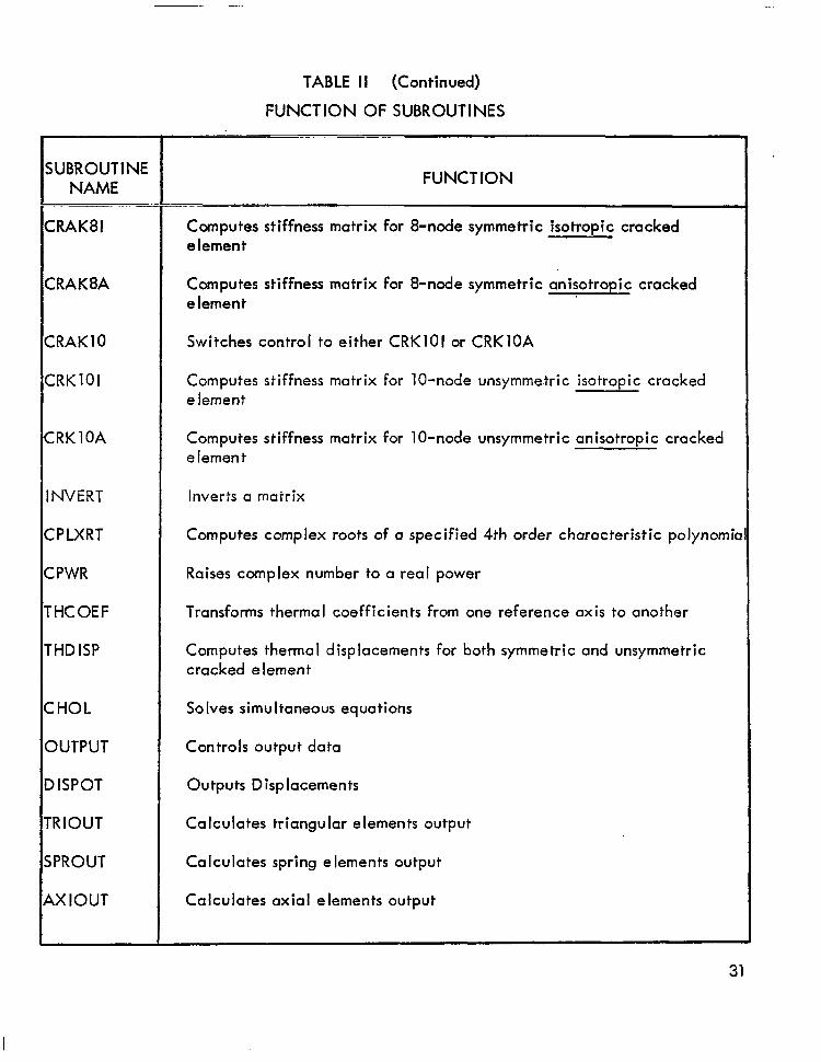
The computer program consists of a main program called CRAK, which allocates the core and calls sequentially four main driver subroutines (INPUT, KFORM, CHOL, OUTPUT), and 32 subroutines. These subroutines have been overlayed to reduce the core required for program code, permanent data, cnd program table. The segment structure of the program i s shown in figure 4. The name and function of each subroutine are given in Table I I .

The input segment of the program contains data generator features to minimize the labor required to input a model. During the input sequence, a banding algorithm i s used to resequence the node numbers to minimize the band-width of the structural stiffness matrix which i s assembled in the KFORM segment. This banding algorithm i s quite effective and helps to minimize execution times. A banded Cholesky decomposition procedure (segment CHOL) i s used to solve the system of equations. The computer program organization i s especially characterized by i t s flexibility of application. The planned segmented structure of the program also makes i t easy to insert additional cracked and conventional e lements as desired.

The scheme of the analysis i s basically divided into the following stages:

Input of geometry, material data and restraints

a Input of applied nodal loads and imposed nodal displacements

4 Calculation of element stiffness matrices

Assembly of element stiffness into a system stiffness

Solution of simultaneous equations for nodal displacements

Output nodal displacements

28

I

Calculation and output of forces (or stresses) in conventional elements

Calculation and output of stress-intensity factors and strain-energy release rates

The overall logic flow of the computer program is depicted in figure 5.

The computer program is efficient in its use of computing time and core storage. Core use can easily be changed to fit individual problem sizes if desired. Full advantage has been taken of symmetry and the banded nature of the simulfaneous equations to be solved, and no data are generated when not required.

29

SUBROUTINE NAME

INPUT

CORIN

TRlN

SPRGIN

4XIN

ZRKIN8

CRKNlO

MATIN

IISPIN

LOAD IN

ZONNEC

3AND IT

3AND

K.FORM

TR I

5PRNG

4x I

ZRAK8

30

TABLE It

FUNCTION OF SUBROUTINES

FUNCTION

Inputs model general specifications

Inputs nadal coordinates and restraints

Inputs triangular elements for both isotropic and anisotropic cases

Inputs spring elements

Inputs axial elements

Inputs 8-node symmetric cracked elements for both isotropic and anisotropic cases

Inputs 10-node unsymrnetric cracked elements for both isotropic and anisotropic cases.

Inputs material properties

Inputs imposed displacements

Inputs applied loads

Generates data which subroutine BANDIT requires

Renumbers the node points to minimize band width

Determines the band-width

Forms a complete stiffness matrix

Computes triangular element stiffness matrix

Computes spring element stiffness matrix

Computes axial element stiffness matrix

Switches control to either CRAK81 or CRAK8A

SUBROUTINE

CRAK81

CRAK8A

CRAK 10

CRKlOl

CRK 1 OA

INVERT

CPLXRT

CPWR

THCOEF

THD ISP

CHOL

OUTPUT

DISPOT

TRIOUT

SPROUT

AXIOUT

TABLE I I (Continued)

FUNCTION OF SUBROUTINES ~~ ~~~ . . ."

FUNCTION "" __ "" ~ -

Computes stiffness matrix for 8-node symmetric isotropic cracked e lement

Computes stiffness matrix for 8-node symmetric anisotropic cracked element

Switches control to either CRKlOl or CRKlOA

Computes stiffness matrix for 10-node unsymmetric isotropic cracked element

Computes stiffness matrix for 10-node unsymmetric anisotropic cracked e lemen t

Inverts a matrix

Computes complex roots of a specified 4th order characteristic polynomia

Raises complex number to a real power

Transforms thermal coefficients from one reference axis to another

Computes thermal displacements for both symmetric and unsymmetric cracked element

Solves simultaneous equations

Controls output data

Outputs Displacements

Calculates triangular elements output

Calculates spring elements output

Calculates axial elements output

31

SUBROUTINE 1 NAME

CRK08

CRKOlO

TABLE I I (Continued)

FUNCTION OF SUBROUTINES

FUNCTION

Calculates K for the 8-node symmetric elements

Calculates K and K for the 10-node unsymmetric elements

I

I I I

32

SAMPLE PROBLEMS

This finite-element computer program has been tested extensively. Both symmetric and unsymmetric cracked elements have performed well with respect to accuracy and efficiency, as shown by sample problems presented here. These results were achieved with a relatively coarse finite-element grid. With refinements in the grid, even more accurate results would be obtained. The symmetric cracked element normally gives more accurate results than the unsymmetric cracked element, which i s understandable in view of the fact that the unsymmetric cracked element has fewer degrees of freedom that it can bring to bear on the first mode. However, the unsymmetric cracked element can be used in a much wider class of crack problems and i s more practical for industrial applications.

To illustrate the capabilities of these two types of crack elements (symmetric and unsymmetric), a number of selected sample problems are included in this report. These sample problems were' chosen to demonstrate (1) the accuracy and economy of the elements, and (2) the versatilities of the elements to perform analyses for structural configurations of p r a c tica I importance.

Anisotropic Case

Center-Cracked and Double-Edge-Cracked Orthotropic Tension Plates - A center- cracked a n i o r a d o u b l e z t e d to uniform tension as solved by Snyder and Cruse (ref. 17) was investigated. The plate analyzed i s 228.6 mm long and 76.2 mm wide. The finite-element models used for both the center- cracked plate and the double-edge-cracked plate are shown in figure 7. The half-crack lengths, a, analyzed are 15.24 rnm and 22.86 mm for the center-cracked plate and 15.24 mm only for the double-edge-cracked plate.

_i- - -. "~

Numerical results were obtained for 10 representative graphite fiber-reinforced epoxy laminates: (0) , c30) , e34) , e45) , e56) , e60) , (90) , (904/f45) , (902/?45)s, (O/f45/90)s0 Lamina properties used were:

S S S S S S S

E l = 144.795 GPa , G12 = 9.653 GPa

E22 = 1 1 .722 GPa , vl* =0.21

Table 111 indicates the complex roots obtained from the characteristic equation for each lam inate.

Results are presented in Tables N, V, and VI. The distribution of differences from Snyder and Cruse's results are summarized in table VII, Notice,that the results generated using &node symmetric cracked element are closer to Snyder and Cruse's results than k e

33

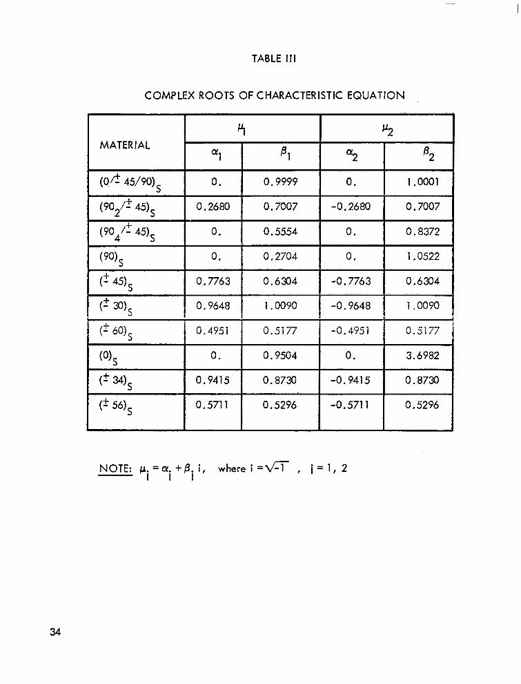
TABLE 1 1 1

COMPLEX ROOTS OF CHARACTERISTIC EQUATION

( 2 m s

(OIs

0.5177 -0.495 1 0.51 77 0,4951 ( 2 bo)*

1.0090 -0.9648 1 .0090 0.9648

0. 0.9504 0.

0.5296 -0.571 1 0.5296 0.571 1 P 5 6 4

0. a730 -0 941 5 0.8730 0.9415 ( 2 w s

3.6982

-~ ~~

NOTE: p. =CY. +8. i f where i = f l , i = 1 2 I l l

34

TABLE IV

.. -~

MATERIAL

STRESS-INTENSITY FACTORS OF CENTER-CRACKED PLATES (a = 15.24 rnrn, a/w =0.4)

SNYDER & CRUSE

KI (MPa - f i )

1.670 _. . -

l.679

- -~ ~~ "~

1.670 .. . .

1.683

1.745 .. . . ~

1.712 . .

1.719 ~~

1.645 ." ~

8-NODE CRACKED ELEMENT

% OFF

1.675

I ,696 +1.01

~

1.702 +1 .F2 " .. . " ". ~ _ _

1.669 -0.83

1.634 -6.36 _ _ ~ "" .." ~ . ~~

1.643 -4.03 "

1.683 -2.09 ~ - . . . . . . . -

1.652 a .43 ~~


K I % OFF

1.622 -2.88

1.652 -1.61

1.671 4.06

1.755 d .28

1.617 -7.34

1.574 -8.06

1.649 -4.07

1.578 -4.07

35

TABLE V

STRESS-INTENSITY FACTORS OF CENTER-CRACKED PLATES (a = 22.86 mm, a/w = 0.6)

SNYDER & CRUSE MATER IA L

KI (MPa - ,/")

(O/f 45/90) " I

2.396

2.396

2.394

2.599

2.518

2.533

I 2.314

.~


T 2.396 +0.01

2.444 4 . 9 1

2.446 +2.(>9 " ~ ~~~ ~~

2.419 +1.04

2.421 -6.85 - . ..

2.405 -4.49

2.473 -2.37

2.336 44.95

- . . . - -. - -


KI ~ .~

2.326

2.389

2.413 "

2.574

2.393 .- ". ~ ~ .

2.302

2.430 P

2.229

% OFF ~~ ~~ ~

-2.92 . ."~ ~

-1.36

"0.71

+7.52

-7.93 ~~~ ~

-8.58

-4.07 ~

-3.67

36

TABLE VI

STRESS- INTENSITY FACTORS OF DOUBLE-EDGE-CRACKED PLATES (a = 15.24 mm, a/w = 0.4)

I MATER IA L

I ~~

SNYDER & CRUSE

K , (MPa - f i )

1.722

1.722

1 . X 6

1.709

1.700

1 .783.

1.717

1.670

1.750 ~-

1.745

T I

8-NODE CRACKED ELEMENT -. -

K I

1.701

1.729

1.725

1.689

1.757

1.722

1.767

1.660

1.737

1.765

% OFF n

-1.22

M.41

+ l . l l

-1.17

+3.35

-3.42

+2.91

-0.60

-0.74 - .

+l .15

I 10-NODE

CRACKED ELEMENT

K I % OFF

1.649 -4.24

1.685 -2.15

1.688 -1.06

1.752 +2.52

1.766 +3.88

1.697 -4.82

1.736 +1.11

1.598 -4.31

1.724 -1.49

1.746 N.06

37

I

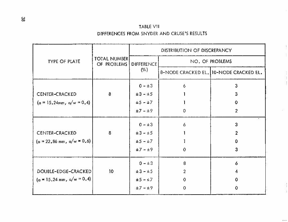
TYPE OF PLATE

CENTER-CRACKED

(a = 15.24mm, a/w = 0.4)

CENTER-CRACKED

(a = 22.86 mm, a/w 0.6)

DOUBLE-EDGE-CRACKED

(a = 15.24 mm, a/w = 0.4)

TABLE V I I DIFFERENCES FROM SNYDER AND CRUSE'S RESULTS

TOTAL NUMBER OF PROBLEMS

8

8

10

DIFFERENCE ("/. )

0-&3

* 3 - A 5 *5 - k 7

& 7 - & 9

0 - k 3

k3 - k 5

*5 - -17

k7 - k9

O-rt3

* 3 - & 5

&5 - 5 7

k 7 - % 9

DISTRIBUTION OF DISCREPANCY

NO. OF PROBLEMS

8-NODE CRACKED EL,

6

1

1

0

6

1

1

0

8

2

0

0

IO-NODE CRACKED EL.

obtained from the 10-node unsymmetric cracked element. Since Snyder and Cruse used the boundary-integral approach, no definite conclusion can be drawn with regard to the abso- lute accuracy of their results. Besides, these finite-element solutions used a large integrcr tion step size (10 steps between nodes) along the boundaries for the numerical integration in forming the stiffness matrix of the cracked element. Accuracy would be improved by re- ducing the integration step size (increasing the number of steps between nodes).

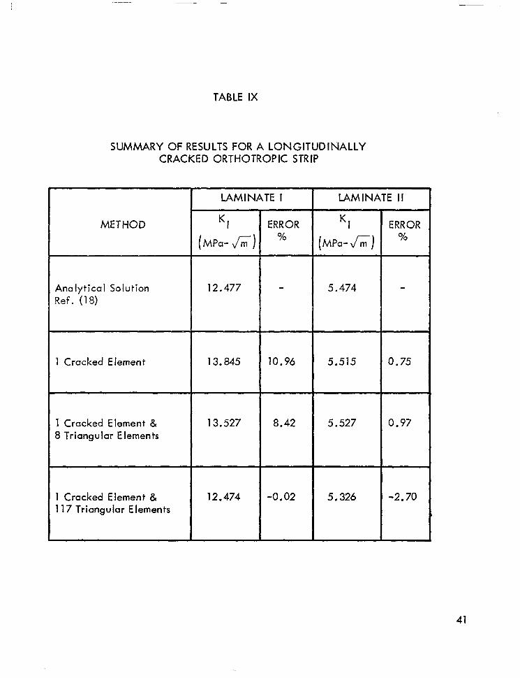
Longitudina I ly Cracked Orthotropic sfrip- The longitudinally cracked orthotropic strip problem as shown in figure 8 was solved under plane-stress and imposed displacement conditions. An analytical solution was developed based upon the energy equivalence and Sih’s results of ref. 18. The solution i s given below as

K,2 =

where a.. = Elements of the material compliance matrix ‘ I

6 = Imposed displacement

h = Height of the plate

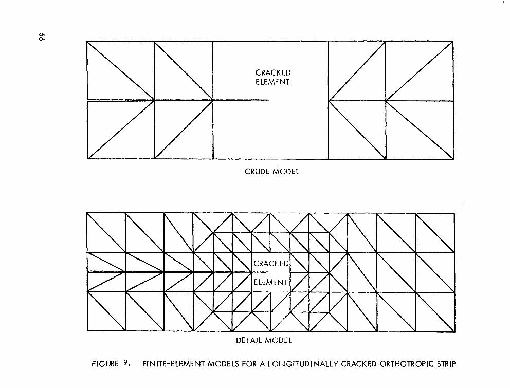
Numerical results were obtained for the two different laminates shown in table VIII. In one case, the laminate i s stiffer in the direction normal to the crack. In the other case, the laminate is-stiffer in the direction of the crack. Both laminate cases were solved using a single cracked element and the two different model representations shown in figure 9 . The results are summarized in table IX.

45-Degree ~~~~ Cracked ~~~~ Finite Orthotropic Plate - This problem i s shown in figure 10. The finite-element model (figure 11) representing this plate consists of 130 nodes, 210 anisotropic triangular elements, and two 10-node anisotropic cracked elements. The problem was solved under uniform remote stress and plane-stress conditions. The stress-intensity factors obtained are given below:

KI = 1.1376 x MPa -6 and KI1 = 1.1784 x MPa -F

Both K I and KII are within f2 percent (-1.77% and +1.75%, respectively) of Sih’s solution, ref. 18, ( K , and KI I = 1.1581 x MPa -JT;;) for an infinite sheet, and they satisfy NASA’s requirement for the accuracy of the program.

39

I

TABLE V l l l

LAMINATE STIFFNESS MATRICES (Scotchply 1002)

I LAM I NATE I I LAMINATE I I I 11 300 0.572 0 34.503 0.572 0 0.572 34.503 0 ]

(GPa) 0 0 4.854 1 0 4.854 [A] = [ 0.572 11 3 0 0 0

NOTE: 10) = [A] { C I ~ - ~ , where x-y refers to the reference coordinates X'Y

!

TABLE IX

"

SUMMARY OF RESULTS FOR A LONGITUDINALLY CRACKED ORTHOTROPIC STRIP

METHOD

Analytical Solution Ref. (18)

1 Cracked E lement

1 Cracked Element & 8 Triangular Elements

1 Cracked Element 8. 117 Triangular Elements

LAM NATE I

K I [ MPa- A)

12.477

13.845

1 3.527

12.474

ERROR %

10.96

8.42

-0.02

LAMINATE II

K I (MPa-

5.474

5.515

5.527

5.326

ERR OR YO

0.75

0.97

-2.70

41

Cracked Tension Plates - Isotropic Case

The sample problem, shown in figure 12, was the first problem analyzed with the symmetric cracked element. I t exhibits the degree of accuracy which has been consistently achieved in numerous subsequent problems. The finite-element model has 30 nodes, 35 triangular elements, and one 8-node symmetric cracked element, The three configurations (the single-edge crack, the double-edge crack, and the center- crack) were all individually analyzed with this one model for an a/w ratio of 1/3. The model grid, which i s quite coarse, results in the single- edge-crack model having 57 displacement degrees-of-freedom (DOF), while the double-edge-crack and center-crack models have 51 DOF. The stress-intensity factors computed using these configurations are compared with ASTM (American Society for Testing and Materials) values. The accuracy of the finite-element predictions are impressive (4 .5% error) for a l l three cases. Refine- ments in the model would produce steady convergence toward ASTM values.

The same cracked problems were solved using an unsymmetric cracked element. The finite-element model as shown in figure 13 consists of 54 nodes, 69 triangular elements, and one 10-node unsymmetric cracked element. The results are not as good as those obtained using the 8-node symmetric cracked element, because the 8-node element has more degrees of freedom to bear on the first node.

An eccentric crack problem as shown in figure 14 was also solved, and the results compared with Isida's solution.

AI I these results are summarized in table X for reference.

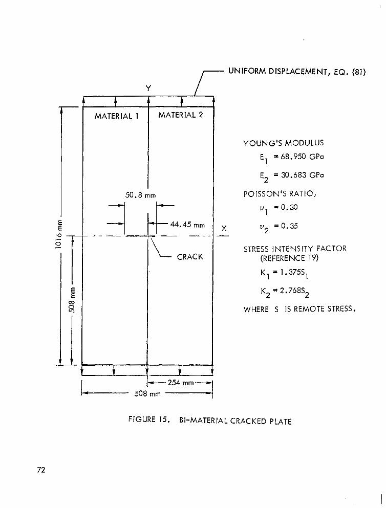
Bi-Material Cracked Plate - This problem, as shown in figure 15, was solved in response to the NASA's Request for Proposal (RFP 1-31-4957), dated 28 May 1974. I t was required that the stress-intensity factors of this isotropic, generalized plane-strain problem must be within 9% of Erdogan's results for an infinite plate (ref. 19). A l l dimensions and material properties are given in figure 15.

In the finite-element model shown in figure 16, only the upper half of the plate has been modeled due to its symmetry with respect to the x-axis. It contains 100 nodes, 148 plane-strain triangles, and 2 eight-node symmetric cracked elements.

A uniform displacement of 46.228 x 10 mm was imposed on the top boundary nodes. -6

This was arrived at as follows. For plane strain, 2 2

H(1 - u1 ) S1 H( l - u2 ) S2 6 = - -

El E2

where H i s the half-height of the finite sheet. S 1 was taken as unity.

42

TABLE X

SUMMARY OF TYPICAL RESULTS FOR ISOTROPIC TENSION PANELS

C RAC K DESCRIPTION

SINGLE EDGE CRACK (a/W = 1/3)

DOUBLE EDGE CRACK (am = 1/3)

CENTER CRACK (a/W = 1/3)

ECCENTRIC CRACK (IS IDA'S PROBLEM)

EIGHT-NODE TEN-NODE SYMMETRIC ELEMENT (ES E) UNSYMMETR IC ELEMENT flUE)

I

F. E. MODEL

68 TRIANGULAR -1.2 35 TRIANGULAR

F. E. MODEL K I % ERROR

ELEMENTS PLUS ELEMENTS PLUS

1 ESE, -1.5

DOF = 105 -HI. 15 DOF =57

1 TUE,

116 TRIANGULAR ELEME.NTS PLUS (SIDE A) i - l o l

NONE

2 ESE,

(SIDE B) DOF = 152

"0.5

c

"

"

i

K , % ERROR

-2.6

-2.6

-1.2

NONE

P w

I

The computed stress-intensity factors for the two crack tips are

K 1 =2,67496 x MPa -F K,2 = 0.25067 x MPa -,/%-

These values include in their definition a factor of K. To compare with the values in the Request for Proposal, i t i s necessary to divide by ,fii; hence,

K1 = 1.50918 x low3 MPa -fi K2 = 0.14143 x MPa -6 These values are quite close to those computed by Erdogan and Biricikoglu in ref. 19, The percentage of error i s -0.12% and +O. 75%, respectively. The axia I stresses and displacements along the crack line are plotted in figures 17 and 18.

Stiffened Plate - The rate of growth of a crack in a stiffened plate w i l l be influenced by the presence of the risers. The simple stiffened plate configuration shown in figure 19 has been analyzed to determine this effect. The plate i s loaded by a stress along its edge normal to the crack. Two cracks are assumed to propagate from the center of the two edges of the plate toward the risers. When the cracks have passed underneath the risers, they are assumed to extend up the riser and into the plate at an equal rate until the riser i s completely fciled. The crack is then assumed to continue t:, propasate into the plate.

Only one quarter of the configuration shown in figure 19 i s idealized, the remainder being represented by symmetric boundary restraints. Both the plate and the riser are idealized using triangular membrane elements. The 8-node crack element i s used to represent the crack tip.

The results of the analysis i s shown in figure 20 in the form of the crack tip symmetric stress-intensity factor plotted against the crack length. It i s evident that the riser w i l l have a considerable effect on the rate of crack growth.

Thermal Stress-Intensity Problem - Sih (ref. 21) has given the following plane-stress formulae for the stress-intensity factors appropriate to a crack with constant-temperature faces (see figure 21) acting as sinks for the steady, radially inward flow of heat Q at infinity.

In (82), a i s the coefficient of thermal expansion, and k i s the thermal conductivity. We now solve the associated temperature-distribution problem to obtain thermal input in a form acceptable to the computer program.

The general real solution for the temperature, T, in a steady heat-conduction problem in two dimensions i s

44

T(x, y) = f(z) + r(z) where f is an analytic function of z = x + iy. The symmetry of the problem indicated in figure 21 permits us to write

which leads at once to

permitting (83) to be written as

T(x, y) = f(z) + f(T)

The constant-temperature condition for the crack faces requires that

" a T - f'(z) + fa'(;) ax

vanish on t he crack faces; i .e.

+ - 2 2 f ' (x) + f ' (x) = 0 , x < a

In (87) and (88), prime (I) denotes differentiation with respect to the parenthetical variable, while the superscript (+) or (-) indicates a value taken in the upper and lower half planes, respectively .

The boundary condition at infinity i s

in which r and 8 (shown in figure 21) are defined by

ie z = re

In view of (89), f'(z) i s expected to vary at infinity like z . - 1

We now make the usual substitution for a cut-condition like (88); i.e.,

g ( 4 =dz* - a 2 fl(z) , (91)

45

2 2 i n w h i c h i z - a i s that branch of ( z - a ) varying like z at infinity. Because of the anticipated remote behavior of f'(z), we expect g(z) to tend to a constant value at infinity.

2 2 1/2

The problem case in terms of g(z) i s then

+ - 2 2 g (x) - g (x) = O , x < a ;

The obvious solution being

which leads to

(94)

(95)

when (91) i s integrated.

The constant c2 in (95) only sets the temperature reference, which i s thus far unspec- ified. Taking c = 0 with no loss in general applicability, we find 2

for large z. Upon imposing (89), we find

- Q - 4kR

Thus, from (86) , (95) , and (97) ,

and the constant crack-face temperature is given by

- Q h a T c - 2k77

(97)

Referring to figure 22, i t i s convenient to let

'1 =4- r - -dm '2 =4-

e, = tan-' x + a

8 = tan - 1 X

e 2 = tan - x - a

- 1 Y

then the temperature distribution can be written as

Figure 23 shows a finite-element representation of the first quadrant of the problem i.n figure 21. The eight-node symmetric cracked element ABCD represents the crack-tip neighborhood in the finite-element model. Input particulars are taken to be

" * - 255.928OK and a = 114.3 mrn k (101)

leading to a crack-face temperature from (99) of

T = 255.505OK C

and triangular-element temperatures (centroidal) from (98).

The computer program was executed twice with additional materra1 properties:

E = 68.95 GPa , u =0.3 and a = 1.8 x 10 m.m .K -6 - 1 -1

(1 03)

In the first execution, the temperature of the cracked element was taken to correspond uniformly to that of the crack faces (102). The computed stress-intensity factor

K I = 4.9137 x MPa -fi ( 1 04)

i s 14.95% higher than the analytical value of 4.2747 x MPa -6. This i s not unexpected in view of the fact that the entire cracked element i s taking the crack-face temperature, a condition thermally more severe than the analytical temperature distribution (98). This i s reflected in the results of the second execution, in which the temperature of the cracked element was taken to be 255.5670Kf which corresponds to the average

47

of six superimposed triangles (shown dashed in figure 23). The stress-intensity factor computed for the second execution was

K I = 3.6325 x MPa -p ( 105)

which is 15% lower than the analytical value. It i s clear that more refinement in the crack-tip neighborhood would lead to a more tolerable discrepancy. It i s important to point out that such refinement w i l l not be necessary in more routine applications where the temperature gradients near the crack tip are less severe.

48

APPENDIX - ELEMENT STIFFNESS.MATRICES

Axial Element

The positive sign convention for the axial element is illustrated in figure A-1 . For this convention k and P,, are as follows:

l r

k]= [: :] , {Prt} = - A E a T

Trianau lar Membrane E lement

The sign convention for the triangular membrane element i s illustrated in figure A-2. Note that six displacements or degrees of freedom are present. It is then reasonable to assume the following displacement field.

u = a , + a x + a y 2 3 v = a 4 + a x + a6y 5

The displacements of the element can then be expressed in terms of the a. coefficients as follows:

I

1

x2

x3

o r in matrix notation

y 3

1

x2

1 x 3

a 1

a2

a3

a4

a5

a6

then

49

where

y3

-x3 x2

x2y3

-y3

x 32

y3

-x3 x2 : where x - 32 - '3 - x2'

The strains can also be expressed in terms of the displacement coefficients:

ou 5, - + r - ;J - -

xy 6 y c x -

Then

If the strains and stresses are constant within the membrane element, the strain energy can be expressed as

s = Aot {u}T { F }

where A is the area of triangular element. Let the stress-strain relations for the anisotropic material In the elemental reference system be written as

0.

50

Then the strain energy can be expressed in terms of the node point displacements as follows:

S = 2 A 0 tk}T[8]T [A] [B] (.}

S = f Aot (d)’ k-’] [BIT [.][B]k”] (6) And the k matrix for the triangular membrane element is, therefore, 11

[k]= Aot k-’]’[B]T [A] [B] [C-’]

If the multiplication i s carried out and i f the elements of the matrix are arranged so that the convention in figure A-3 applies then the k.. elements of the stiffness matrix are

‘I

( . ) k12 = y3 A13 - ’3 x32 (A12 + A33) + x322 A23 2

(>) k14=-Y3 A 1 3 + X 3 Y 3 A 1 2 f Y 3 X 3 2 A 3 3 - X 3 X 3 2 A 2 3 2

(7) k23 = - y3 A1 3 + x3 y3 A33 + y3 x32 *12 - x3 x32 A23 2

51

(>) k24 - - -Y: ~ 3 3 + Y3 (x3 + x321 ~ 2 3 - x3 x32 ~ 2 2

(:) k25 = x2 '32 A23 - x2 '3 A33

('a\ k26 = x2 x32 A22 - x2 '3 A23

(:) k33 - y3 Al 1 - 2x3 y3 A13 + x 3 A33

(:) k 3 4 - Y 3 A13

(>) k35 =x2 y3 A13 - X 2 X 3 A 33

- 2 2

2 2 - - x3 y3 (A12 + A33) + x3 A23

k36=X2 y3 A12 2 3 23 - X X A

(>) k44-Y3 33 - 2 A - 2 x y A + x 2 A

3 3 23 3 22

(>) k45 = -x 2 x 3 A 23 + x 2 y3 A33

(?) k46 2 3 22 2 3 23 = - X X A + X y A

(T) 4Ao k55 - - x2 2 A33

2 (>) k56 - x2 A23

(>) k66 - '2 A22

-

- 2

52

1 0 - TX2'3 where A -

x32 - '3 - '2 -

The values of Prt for the triangular plate element can be computed in terms of the element stiffness matrix. Note that

If { PI = 0 and { p 1 i s selected as the thermal displacemen t for free expansion, then the forces for complete restraint are

For the triangular plate element, the components of

u, = o

v, = o

v2 = o

The symbol * implies that the thermal expansion coefficients have been rotated into the local reference axis for the element.

Spring or Fastener Element

Figure A-4 illustrates two plates connected by a shear pin, and the direction vectors for the system of forces that are assumed to act on the pin are i Ilustrated in figure A-5. For the spring element, i t i s necessary to define four node points. Node points ('I) and (2) define the element itself. In most structural models these node points may be coincident before any strains occur, that is, (Z, - Z2) = 0. Node points (3) and (4) are used in conjunction with node point (1) to define direction vectors for spring elements K1 and K2, respectively. Kg i s assumed to be a spring element perpendicular to the plane containing K1 and K2. In other words, the system of spring elements i s that illustrated in figure A-6. If we let u, v, w, be displacements, the element forces for the spring system are

53

P = K1 (ul - u2) P = K2 (vl - v2)

x1

Y l

Pzl = K3 (wl - w2)

x1 Px2 = -P

P = -P

= -p Y2 Yl

pz2 zl

Hence, the stiffness matrix i s

LkI =

K 1 0

0 K2

0 0

-K1 0

0 - K2

0 0

0

0

0

0

-K3

-K 0 1

0 -K2

0 0

K 1 0

0 K2

0 0

- 0

0

-K3

0

0

- where K1, K , and K are linear spring stiffnesses for the fastener element.

10-Node Cracked Element Thermal Effects

2 3

Let the coordinate system for the ten node cracked element be the one illustrated in figure A-7. The stress-strain law can be written as

54

Assume a constant temperature distribution over the element; then, for free expansion

and

The displacement function i s then of the form

u = a Tx + C2 a12 Ty + C1 1 1

v = a22Ty + C4 a12 Tx + C 3

If u, = v, - v 6 - = 0, the displacement functions become

u =a1 lTx + a12Ty

As in the case of the triangular plate element

where the element of p are 0

u1 = 0 v3 = - c Y ~ ~ T A

v1 = 0 u 4 = - a T A 12

22 u2 = -a1 l T A v 4 = - a T A

v2 = 0 u5 = CY^ T A - c Y , ~ T A

u3 =-a T A - C Y T A 11 12 v5 - -?*T A -

55

I

u6 =a1 l T A

V6 = 0

u7 1 1 = a T A + o ! , ~ T A

v7 = ' Y ~ ~ T A

u 8 = a T A 12

v8 = a22T A

~9 =-dl I T A +O!I2TA

v 9 = a T A

u , ~ = -al T A

22

y o = 0

56

REFERENCES

1 . Kobayashi, A. S., et al.: Application of the Method of Fini te Element Analysis to Two-Dimensional Problems in Fracture Mechanics. ONR Contract Nonr-477(39), NR 064 478, TR No. 5, University of Washington, Department of Mechanical Engineering, October 1968.

2. Chan, S. K.; Tuba, 1 . S.; and Wilson, W. K.: On the Finite Element Method in Linear Fracture Mechanics. J. o f Eng. Fracture Mechanics, Vol. 2, No. 1, July 1970, pp. 1-17.

3. Oglesby, J. J .; and Lomacky, 0.: An Evaluation of Finite Element Methods for the Computation of Elastic Stress Intensity Factors. Navy Ship Research and Develop- ment Center, NAVSHIPS Project SF 35.422.210, Task 15055, Report No. 3751, December 1971 .

4. Byskov, E.: The Calculation of Stress Intensity Factors Using the Finite Element Method with Cracked Elements. International Journal of Fracture Mechanics, Vol. 6, No. 2, June 1970, pp. 159-167.

5. Tracey, 0. M.: Finite Elements for Determination of %rack Tip Elastic Stress Intensity Factors. Engineering Fracture Mechanics, Vol . 3, 1971, pp . 255-265.

6. Walsh, P. F.: The Computation of Stress Intensity Factors by a Special Finite Element Technique. Internal Journal of Solids and Structures, Vol. 7, 1971, pp. 1333- 1 342.

7. Creager, M.: Development of a Cracked Finite Element. Lockheed-California Company Report, LR23996, December 1970.

8. Pian, T. H. H., et al.: Elastic Crack Analysis by a Finite Element Hybrid Method. Massachusetts Institute of Technology, Air Force Off ice of Scientific Research Con trac t F44620-674 -001 9.

9. Wilson, W. K .: Crack Tip Finite Elements for Plane Elasticity. Westinghouse Research Laboratories Scientific Paper 71-1E7, FMPWR-P2, June 7, 1971.

10. Aberson, J . A.: Cracked Finite Element Development at Lockheed-Georgia Company. LG73ER0007, Lockheed-Georgia Company, September 17, 1973.

11. Tsai, S. W.; and Hahn, H. T.: Recent Developments in Fracture of Filamentary Composites. Proceedingsof an International Conference on Prospects of Fracture Mechanics, June 24-28, 1974, pp. 493-508.

12. Martin, H. C.: Introduction to Matrix Methods of Structural Analysis. McGraw-Hill

57 Book Company, Inc ., New York, 1966.

13.

14.

15.

16.

17.

18.

19.

20.

21.

Przemieniecki, J . S.: Theory of Matr ix Structural Analysis. McGraw-Hi11 Book Company, Inc . , New York, 1968.

Williams, M. L.: Stress Singularities Resulting from Various Boundary Conditions in Angular Comers of Plates in Extension. J . of Applied Mechanics, Vol . 19, December 1952, pp. 526-528.

Williams, M. L.: On the Stress Distribution at the Base of a Stationary Crack. J. of Applied Mechanics, Vol. 24, No. 1, March 1957, pp. 109-114.

Paris, P. C .; and Sih, G. C.: Stress Analysis of Cracks. Fracture Toughness Testing and I t s Application, ASTM STP 381, pp. 60.

Snyder, M. D.; and Cruse, T. A.: Crack Tip Stress intensity Factors in Finite Anisotropic Plates. Air Force Materials Laboratory, AFML-TR-73-209, August 1973.

Sih, G. C.; Paris, P. C.; and Irwin, G. R.: On Cracks in Rectilinearly Anisotropic Bodies. international J. of Fracture Mechanics, Vol. 1, No . 3, 1965, pp. 189- 202.

Erdogan, F.; and Biricikoglu, V.: Two Bonded Half Planes with a Crack Going T I I ;]rough the Interface. Internufional J . of Engiaeering Sciznce, Vol . 2 , No. 7 ,

July 1973.

Wilhem, D. P.: Fracture Mechanics Guidelines for Aircraft Structural Applications. Air Force Flight Dynamics Laboratory, AFFDL-TR-69-111 , February 1970.

Sih, G. C.: On the Singular Character of Thermal Stresses Near a Crack Tip. Journal of Applied Mechanics, Vol . 29, No. 3, September 1962, pp. 587-589.

58

I

FIGURE 1 . TR1ANGULA.R ELEMENT MATERIAL AXIS

~-

FIGURE 2. CRACK-TIP NEIGHBORHOOD

59

(a) 8-node Symmetric Cracked Element

(b) 10-node Unsymmetric Cracked Element

FIGURE 3. CRACKED FINITE ELEMENTS

60

I I I

I LEVEL0 LEVEL 1 I I

CRA K LEVEL 2

I I I I LEVEL3 8 LEVEL4 1

I I I

-. lNPUT

CORIN, DISPIN, LOAD!N, MATIN

TRIN, SPRGIN, AXIN, CRKINS, I CRI<N10, CONNEC

KFORM I BAND, BAN DIT >

CRAK8, CRAKlO . TRI SPRNG THCOEF (A)

A>( I CRA K8 I - - THCOEF (A)

INVERT (I, A) CRAK8A

C R I.< 1 0 .I CR i< 10.4

THDISP (I, A) CPLXRT IA I CHOL [ CF'WR (A)

, OUTPUT

Dl SPOT TRiOLlT

NOTE: SPROUT THCOEF (A) (I) - ISOTROPIC

CRK9T3 -. (A) - ANISOTROPIC

AXIOUT

c R Kc:) 1 0

FIGURE 4. SEGMENT STRUCTURE FOR COMPUTER PROGRAM

Read problem t i t le and control data

t Input nodal points and restraints

1

Input element specifications

1 ~

Input material properties

Input applied nodel loads, or imposed nodel displacements, or temperature distributions

i Calculate bandwidth

I

Compute element stiffness matrices I

1 1

Assemble system stiffness 1 Y

Ca Icu la te and Print noda I displacements I v - - - ~

Calculate and print element forces or stresses ~~

I

Calculate and print

# Nodal equilibrium check

FIGURE 5 . OVERALL LOGIC FLOW OF COMPUTER PROGRAM

62

CENTER CRACK

-f 30.48 (or 45.72 mm)

t- 76.2 rnm-

228.6 m m ”.

t’

DOUBLE-EDGE CRACK

15.24-mm 15.24 mm

FIGURE 6. CENTER-CRACKED AND DOUBLE-EDGE-CRACKED ORTHOTROPIC TENSION PLATE

63

8-NODE SYMMETRIC CRACKED ELEMENT

\ \ / \\

10-NODE UNSYMMETRIC CRACKED ELEMENT

CRACKED E i Z , f A E N T ~

FIGURE 7. CRACKED ORTHOTROPIC TENSION PLATE FINITE-ELEMENT MODELS

64

\ IMPOSED DISPLACEMENT (6) = 0.254 rnrn

1 ""."A """""" - I

FIGURE 8. A LONGITUDINALLY CRACKED ORTHOTROPIC STRIP

0. 0.

CRUDE MODEL

FIGURE 9 . FINITE-ELEMENT MODELS FOR A LONGITUDINALLY CRACKED ORTHOTROPIC STRIP

- 9

0 -7 L

CRACK

UNIFORM STRESS, S = 6.895 x 10' MPa

ELASTIC CONSTANTS:

E,,'= 82.74 GPa

E22 = 24,1325 GPa

G12 = 20,685 GPa

THE PRINCIPAL AXIS OF ORTHOTROPY IS THE Y-AX 1 S

-X

FIGURE 10. 45" CRACKED FINITE ORTHOTROPIC PLATE

67

FIGURE 11. 45' CRACKED ORTHOTROPIC PLATE FINITE-ELEMENT MODEL

68

I=+ FINITE MODEL

FINITE ELEMENT MODEL

KI % ERROR = -1.5

K , % ERROR = 4-0.15

FINITE ELEMENT MODEL = 57 OOF, 35 CONSTANT-STRAIN TRIANGLE

FIGURE 12. SYMMETRIC CRACKED ELEMENT MODEL FOR SINGLE-EDGE, DOUBLE-EDGE, AND CENTER CRACKED TENSION PANELS (a/w = 1/3)

KI % ERROR = -2.6%

10-NODE - UN SYMMETR IC E L E M E N T El KI % ERROR = -2.6%

K, % ERROR = - 1 . 2 %

DOF = 105

E L E M E N T S = 69

FIGURE 13. UNSYMMETRIC CRACKED ELEMENT MODEL FOR SINGLE-EDGE, DOUBLE-EDGE, AND CENTER CRACKED TENSION PANELS ( d w = 1/3)

70

K , % ERROR

= - 1 . 1

F

" I DOF = 152 ELEMENTS = 113

IGURE 14.

+ + + + + t +

ECCENTR IC CRAC

K, % ERROR

= 4-0.5

K (ISIDA'S PROBLEM) MODEL WITH TWO 8-NODE CRACKED ELEMENTS

E E

MATERIAL 1

50.8 mrn

I

MATERIAL 2

t- 44.45 mrn " ". \

X -

UNIFORM DISPLACEMENT, E Q . (81)

YOUNG'S MODULUS

El = 68.950 GPa

E2 = 30.683 GPa

POISSON'S RATIO,

v ~ 0 . 3 0 1

v2 = 0.35

STRESS INTENSITY FACTOR (REFERENCE 19)

K1 = 1.375S1

K2 = 2. 768S2

WHERE S IS REMOTE STRESS.

FIGURE 15. BI-MATERIAL CRACKED PLATE

72

s/s 1 S/S* 3 + '3

I I 2 - - 2

1 I 1 ' F q ' 1

I I 0 I I L L I I

-200 -100 0 100 200

FIGURE 17. STRESS IN BI-MPTERIAL CRACKED PLATE

~ - 0

X (rr#rn)

0 I

-40 - 30 -20 -10 0 X ( m d

FIGURE 18. DISPLACEMENTS OF CRACKED FACES IN B I-MATER IA L PLATE

100

50

0

74

FIIqITE ELEMENT -/ -m a e’---

- 40.64 *-- LITERATURE

68.95 MPa

FINITE ELEMENT

ASSUMING THAT FROM

AND PLATE CRACKS GROW AT THE SAME RATE

1 1

20 1 1 I 1 1 I . I

24 28 32 36 40 44 48 52 I

CRACK LENGTH, CI (mm)

FIGURE 20. EFFECT OF RISER ON STRESS INTENSITY IN PLATE

Y

X

Q

F I G U R E 21. G E O M E T R Y OF THE THERMAL STRESS P R O B L E M

Y

X -a +a

F I G U R E 22, V E C T O R R E P R E S E N T A T I O N FOR T H E R M A L P R O B L E M

77

. . .. ... .. _." - . . . . . - ... - .. . .. .. . . .. .- -- .. ..- ... . -.

Y

X 1 - I

F I G U R E 23. F I N I T E - E L E M E N T R E P R E S E N T A T I O N OF T H E R M A L STRESS P R O B L E M

78

FIGURE A-1. AXIAL ELEMENT

Y

v 1

"9 3

u2

FIGURE A-2. TRIANGULAR ELEMENT MEMBRANE DISPLACEMENTS

6

FIGURE A-3. CONVENTION FOR DEGREES OF FREEDOM

79

NODE

NODE

FIGURE A-4. SHEAR PIN

FIGURE A-5. DIRECTION VECTORS

L

FOR FASTENER ELEMENT

80

. . .. "" - ""

FIGURE A-7. LOCAL COORDINATE SYSTEM FOR TEN-NODE CRACKED ELEMENT

NASA-Langley, 1976 CR-2698 81

finite element computer program analyze … · most widely used membrane element: the...

Documents