finite difference method spatial and time discretization...
TRANSCRIPT

MSE 3050, Phase Diagrams and Kinetics, Leonid Zhigilei
Solutions to the diffusion equation
Numerical integration (not tested)
● finite difference method
● spatial and time discretization
● initial and boundary conditions
● stability
Analytical solution for special cases
● plane source
● thin film on a semi-infinite substrate
● diffusion pair
● constant surface composition
MSE 3050, Phase Diagrams and Kinetics, Leonid Zhigilei
Numerical integration of the diffusion equation (I)Finite difference method. Spatial Discretization. Internal nodes.
RiiLiii
ti
tti AJAJV
t
CC11
Δ
Δ
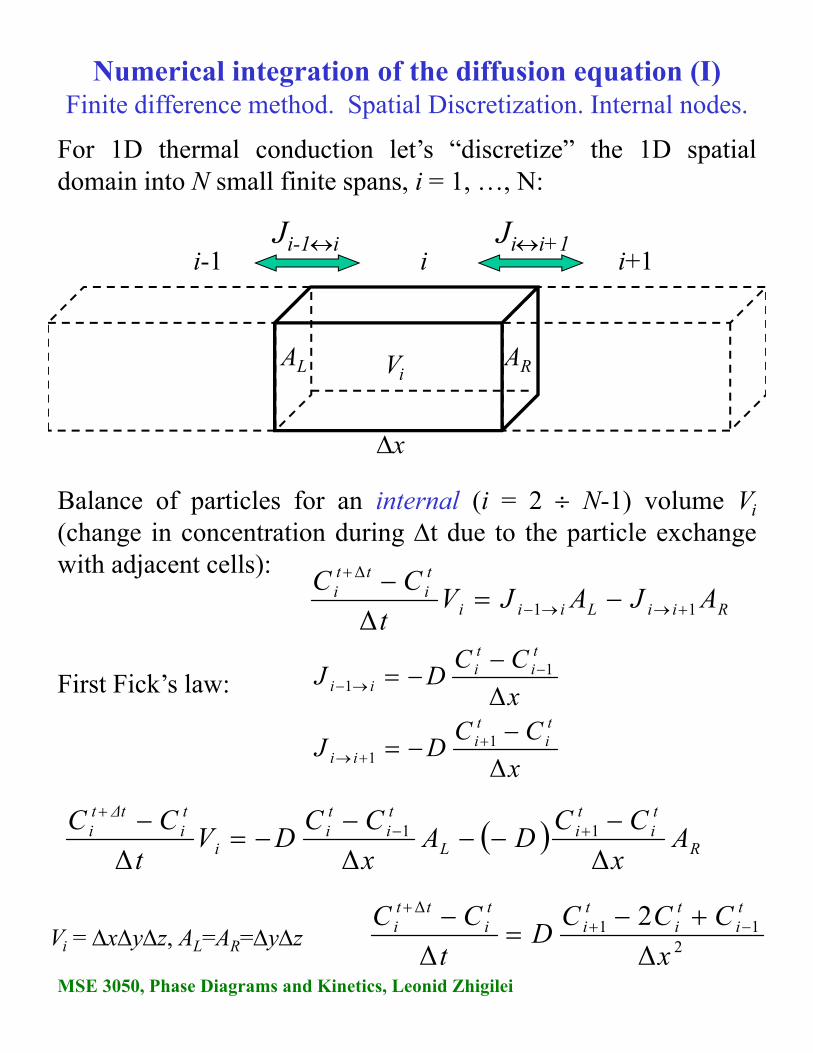
For 1D thermal conduction let’s “discretize” the 1D spatialdomain into N small finite spans, i = 1, …, N:
Balance of particles for an internal (i = 2 N-1) volume Vi
(change in concentration during t due to the particle exchangewith adjacent cells):
x
Vi
Jii+1
ARAL
i-1 i i+1Ji-1i
x
CCDJ
ti
ti
ii Δ1
1
x
CCDJ
ti
ti
ii Δ1
1
R
ti
ti
L
ti
ti
i
ti
Δtti A
x
CCDA
x
CCDV
t
CC
ΔΔΔ11
Vi = xyz, AL=AR=yz
First Fick’s law:
211
Δ
Δ
2
Δ x
CCCD
t
CC ti
ti
ti
ti
tti
MSE 3050, Phase Diagrams and Kinetics, Leonid Zhigilei
Numerical integration of the diffusion equation (II)Finite difference method. Spatial Discretization. Internal nodes.
211
Δ
2
Δ x
CCCD
t
CC ti
ti
ti
ti
Δtti
211Δ
Δ
2Δ
x
CCCDtCC
ti
ti
tit
itt
i
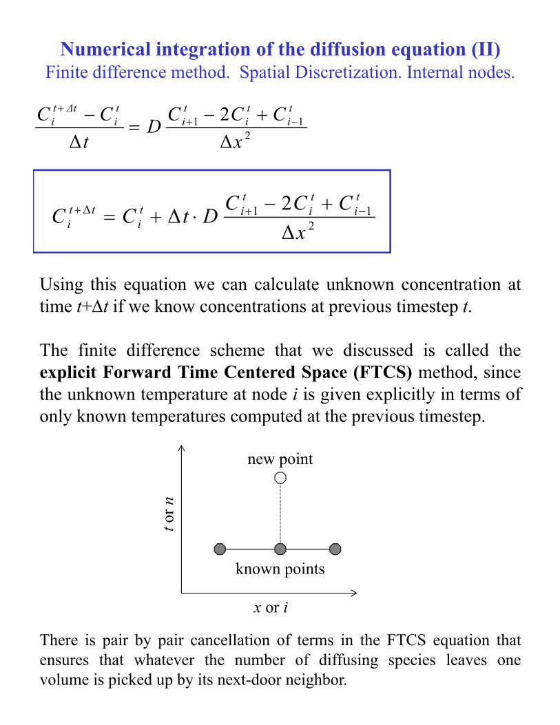
Using this equation we can calculate unknown concentration attime t+t if we know concentrations at previous timestep t.
The finite difference scheme that we discussed is called theexplicit Forward Time Centered Space (FTCS) method, sincethe unknown temperature at node i is given explicitly in terms ofonly known temperatures computed at the previous timestep.
x or i
tor
n
known points
new point
There is pair by pair cancellation of terms in the FTCS equation thatensures that whatever the number of diffusing species leaves onevolume is picked up by its next-door neighbor.
MSE 3050, Phase Diagrams and Kinetics, Leonid Zhigilei
Numerical integration of the diffusion equation (III)Finite difference method. Spatial Discretization. End nodes.
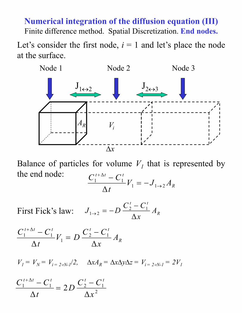
Let’s consider the first node, i = 1 and let’s place the nodeat the surface.
x
Vi
J23
AR
Node 1 Node 2 Node 3
J12
Balance of particles for volume V1 that is represented bythe end node:
R
ttt
AJVt
CC211
1Δ
1
Δ
R
tt
Ax
CCDJ
Δ12
21
R
ttttt
Ax
CCDV
t
CC
ΔΔ12
11
Δ1
First Fick’s law:
V1 = VN = Vi = 2N-1/2, xAR = xyz = Vi = 2N-1 = 2V1
2121
Δ1
Δ2
Δ x
CCD
t
CC ttttt
MSE 3050, Phase Diagrams and Kinetics, Leonid Zhigilei
Numerical integration of the diffusion equation (IV)Finite difference method. Spatial Discretization. End nodes.
212
1Δ
1 Δ2Δ
x
CCDtCC
ttttt
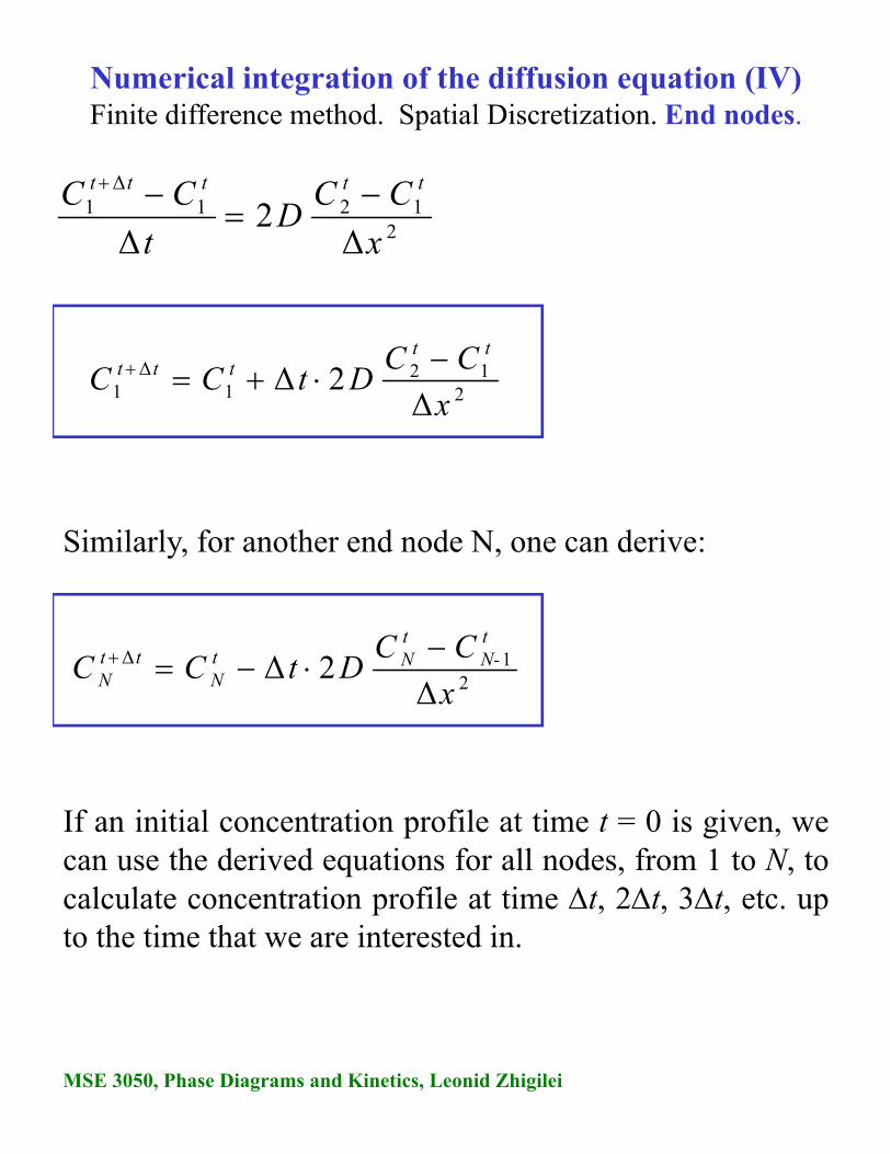
Similarly, for another end node N, one can derive:
2121
Δ1
Δ2
Δ x
CCD
t
CC ttttt
21Δ
Δ2Δ
x
CCDtCC
tN-
tNt
Ntt
N
If an initial concentration profile at time t = 0 is given, wecan use the derived equations for all nodes, from 1 to N, tocalculate concentration profile at time t, 2t, 3t, etc. upto the time that we are interested in.
MSE 3050, Phase Diagrams and Kinetics, Leonid Zhigilei
Stability criterion
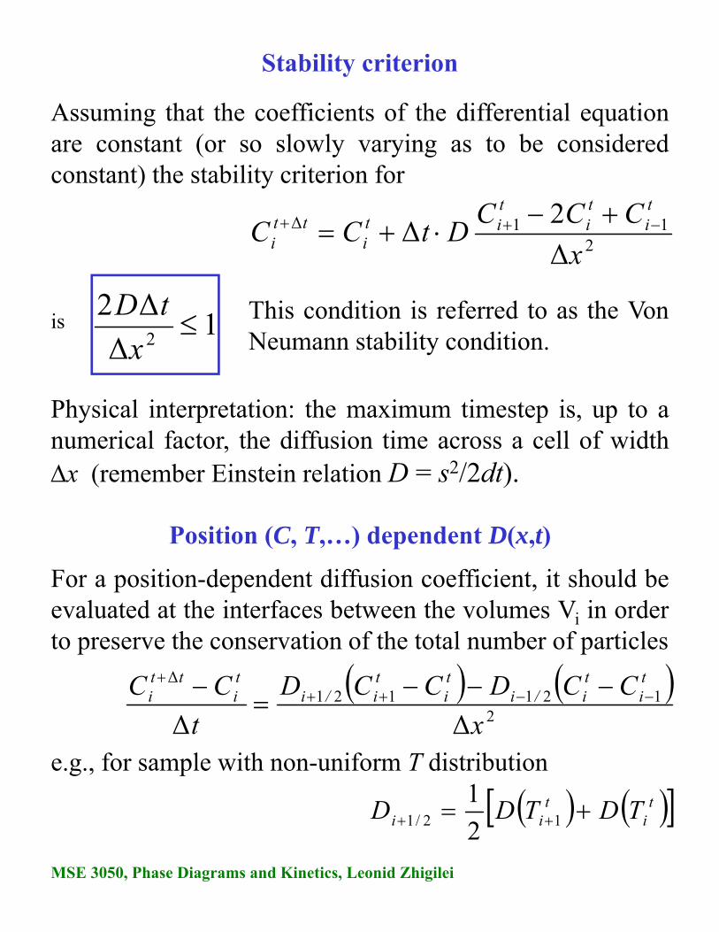
For a position-dependent diffusion coefficient, it should beevaluated at the interfaces between the volumes Vi in orderto preserve the conservation of the total number of particles
e.g., for sample with non-uniform T distribution
ti
tii TDTDD 12/1 2
1
211Δ
Δ
2Δ
x
CCCDtCC
ti
ti
tit
itt
i
2
121121Δ
ΔΔ x
CCDCCD
t
CC ti
ti/i
ti
ti/i
ti
tti
Position (C, T,…) dependent D(x,t)
Assuming that the coefficients of the differential equationare constant (or so slowly varying as to be consideredconstant) the stability criterion for
is 1Δ
Δ22
x
tD
Physical interpretation: the maximum timestep is, up to anumerical factor, the diffusion time across a cell of widthx (remember Einstein relation D = s2/2dt).
This condition is referred to as the VonNeumann stability condition.

MSE 3050, Phase Diagrams and Kinetics, Leonid Zhigilei
0
Lxx
C
No mass transfer through the boundary:
Constant concentration at the boundary CL = Cf and we canuse the following boundary condition:
fLxCC
Simple boundary conditions
N-2 N-1 N N+1
JNN+1= 0
fictive node
CN CN+1 = CN
MSE 3050, Phase Diagrams and Kinetics, Leonid Zhigilei
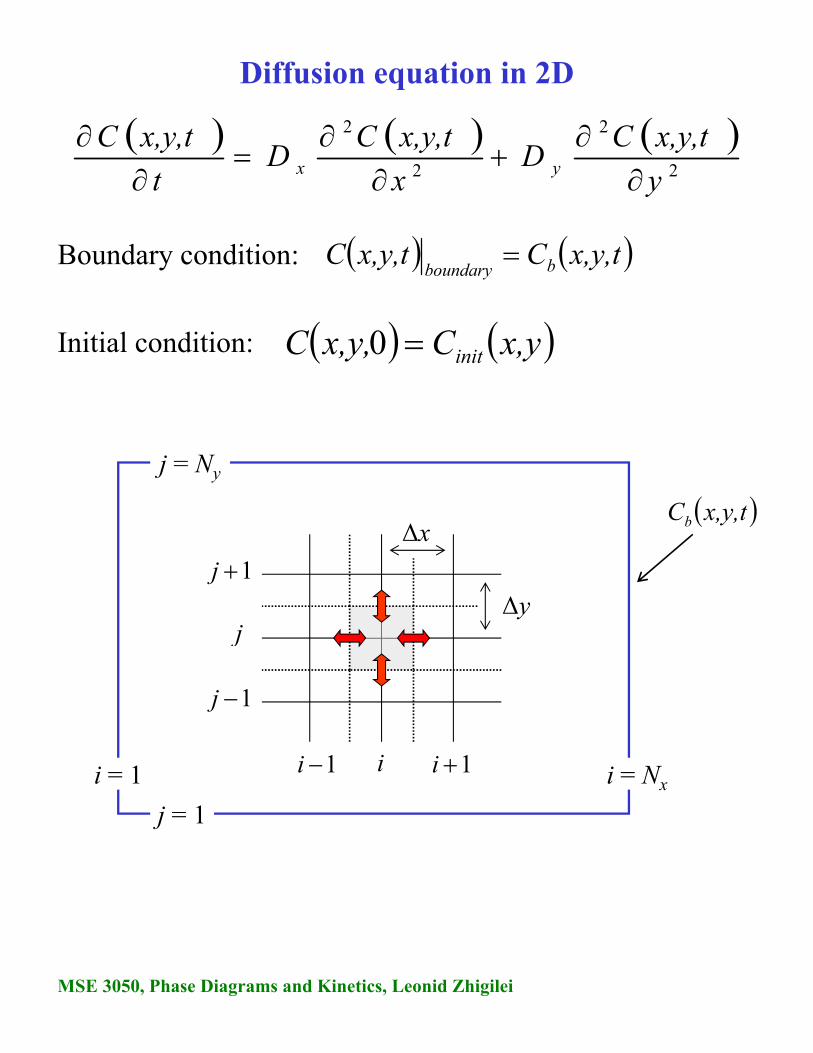
Diffusion equation in 2D
2
2
2
2
y
x,y,tCD
x
x,y,tCD
t
x,y,tCyx
Boundary condition: x,y,tCx,y,tC bboundary
x,yCx,y,C init0Initial condition:
x,y,tCb
i1i 1i
1j
j
1jyΔ
xΔ
i = 1 i = Nx
j = 1
j = Ny

MSE 3050, Phase Diagrams and Kinetics, Leonid Zhigilei
Diffusion equation in 2D: explicit FTCS scheme
2
2
2
2
y
x,y,tCD
x
x,y,tCD
t
x,y,tCyx
t
,jiti,j
t,ji
x
ti,j
tti,j CCC
x
D
t
CC112
Δ
2ΔΔ
t
,jiti,j
t,ji
xti,j
tti,j CCC
x
tDCC 112
Δ 2Δ
Δ
2
1
Δ
Δ
Δ
Δ22
y
tD
x
tD yxStability:
tD~r D Δ4Δ 2
ti,j
ti,j
ti,j
y CCCy
D112
2Δ
ti,j
ti,j
ti,j
y CCCy
tD112
2Δ
Δ

MSE 3050, Phase Diagrams and Kinetics, Leonid Zhigilei
Diffusion equation in 3D: explicit FTCS scheme
t
,j,kiti,j,k
t,j,ki
x
ti,j,k
tti,j,k CCC
x
D
t
CC112
Δ
2ΔΔ
2
2
x
x,y,z,tCD
t
x,y,z,tCx
t
,j,kiti,j,k
t,j,ki
xti,j,k
tti,j,k CCC
x
tDCC 112
Δ 2Δ
Δ
2
1
Δ
Δ
Δ
Δ
Δ
Δ222
z
tD
y
tD
x
tD zyxStability:
tDr D 6~3
2
2
2
2
z
x,y,z,tCD
y
x,y,z,tCD zy
ti,j,k-
ti,j,k
ti,j,k
zt,ki,j
ti,j,k
t,ki,j
y CCCz
DCCC
y
D112112
2Δ
2Δ
ti,j,k-
ti,j,k
ti,j,k
zt,ki,j
ti,j,k
t,ki,j
y CCCz
tDCCC
y
tD112112
2Δ
Δ2
Δ
Δ
MSE 3050, Phase Diagrams and Kinetics, Leonid Zhigilei
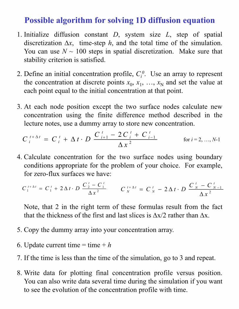
Possible algorithm for solving 1D diffusion equation
1. Initialize diffusion constant D, system size L, step of spatialdiscretization x, time-step h, and the total time of the simulation.You can use N ~ 100 steps in spatial discretization. Make sure thatstability criterion is satisfied.
3. At each node position except the two surface nodes calculate newconcentration using the finite difference method described in thelecture notes, use a dummy array to store new concentration.
2. Define an initial concentration profile, Ci0. Use an array to represent
the concentration at discrete points x0, x1, …, xN and set the value ateach point equal to the initial concentration at that point.
5. Copy the dummy array into your concentration array.
211 2
x
CCCDtCC
ti
ti
tit
itt
i
for i = 2, …, N-1
4. Calculate concentration for the two surface nodes using boundaryconditions appropriate for the problem of your choice. For example,for zero-flux surfaces we have:
212
11 2x
CCDtCC
ttttt
212
x
CCDtCC
tN
tNt
Ntt
N
Note, that 2 in the right term of these formulas result from the factthat the thickness of the first and last slices is x/2 rather than x.
7. If the time is less than the time of the simulation, go to 3 and repeat.
6. Update current time = time + h
8. Write data for plotting final concentration profile versus position.You can also write data several time during the simulation if you wantto see the evolution of the concentration profile with time.
MSE 3050, Phase Diagrams and Kinetics, Leonid Zhigilei
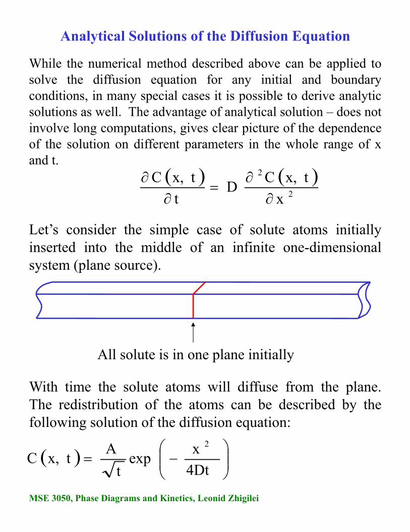
While the numerical method described above can be applied tosolve the diffusion equation for any initial and boundaryconditions, in many special cases it is possible to derive analyticsolutions as well. The advantage of analytical solution – does notinvolve long computations, gives clear picture of the dependenceof the solution on different parameters in the whole range of xand t.
Analytical Solutions of the Diffusion Equation
2
2
x
tx,CD
t
tx,C
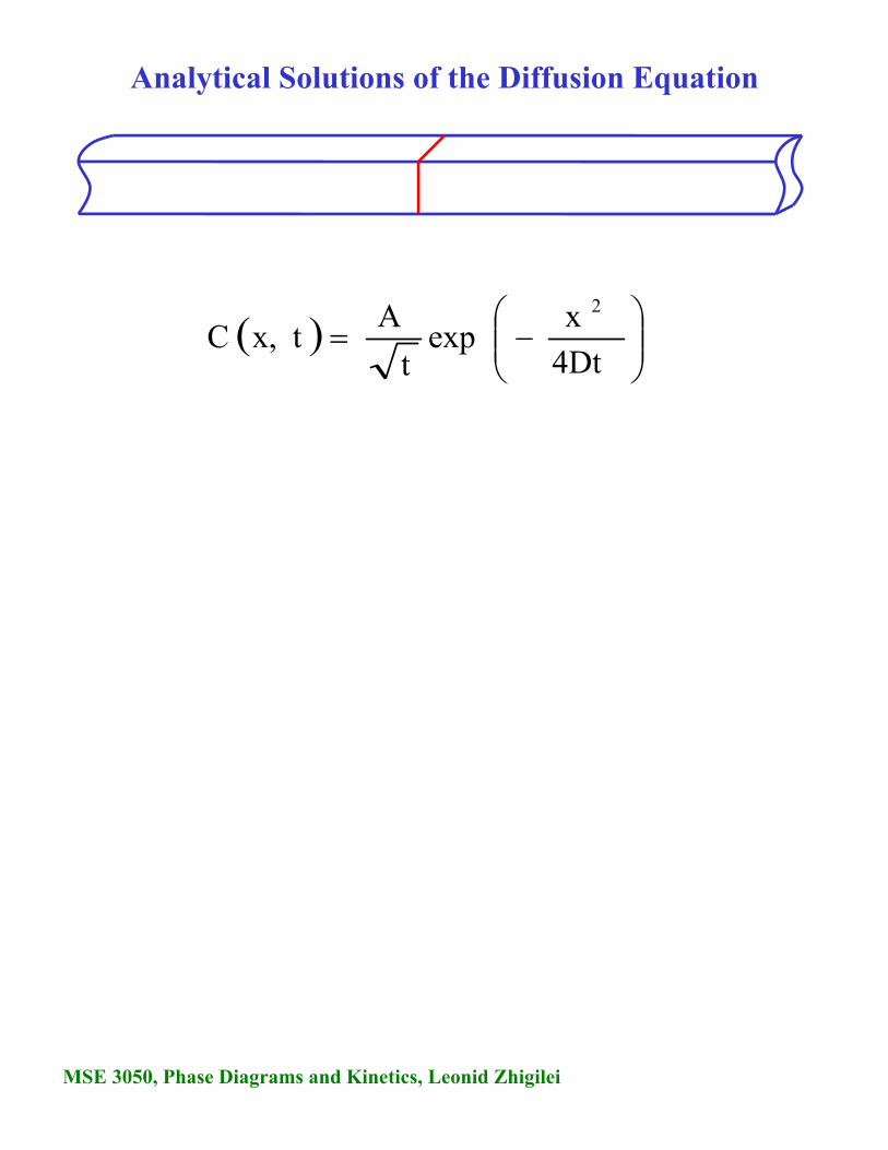
Let’s consider the simple case of solute atoms initiallyinserted into the middle of an infinite one-dimensionalsystem (plane source).
All solute is in one plane initially
With time the solute atoms will diffuse from the plane.The redistribution of the atoms can be described by thefollowing solution of the diffusion equation:
4Dt
xexp
t
Atx,C
2

MSE 3050, Phase Diagrams and Kinetics, Leonid Zhigilei
Analytical solution for plane source
2
2
x
tx,CD
t
tx,C
We can show by differentiation that for the plane source inan infinite system
4Dt
xexp
t
Atx,C
2
is the solution of thediffusion equation
MSE 3050, Phase Diagrams and Kinetics, Leonid Zhigilei
Analytical Solutions of the Diffusion Equation
4Dt
xexp
t
Atx,C
2
MSE 3050, Phase Diagrams and Kinetics, Leonid Zhigilei
Analytical solution for plane source
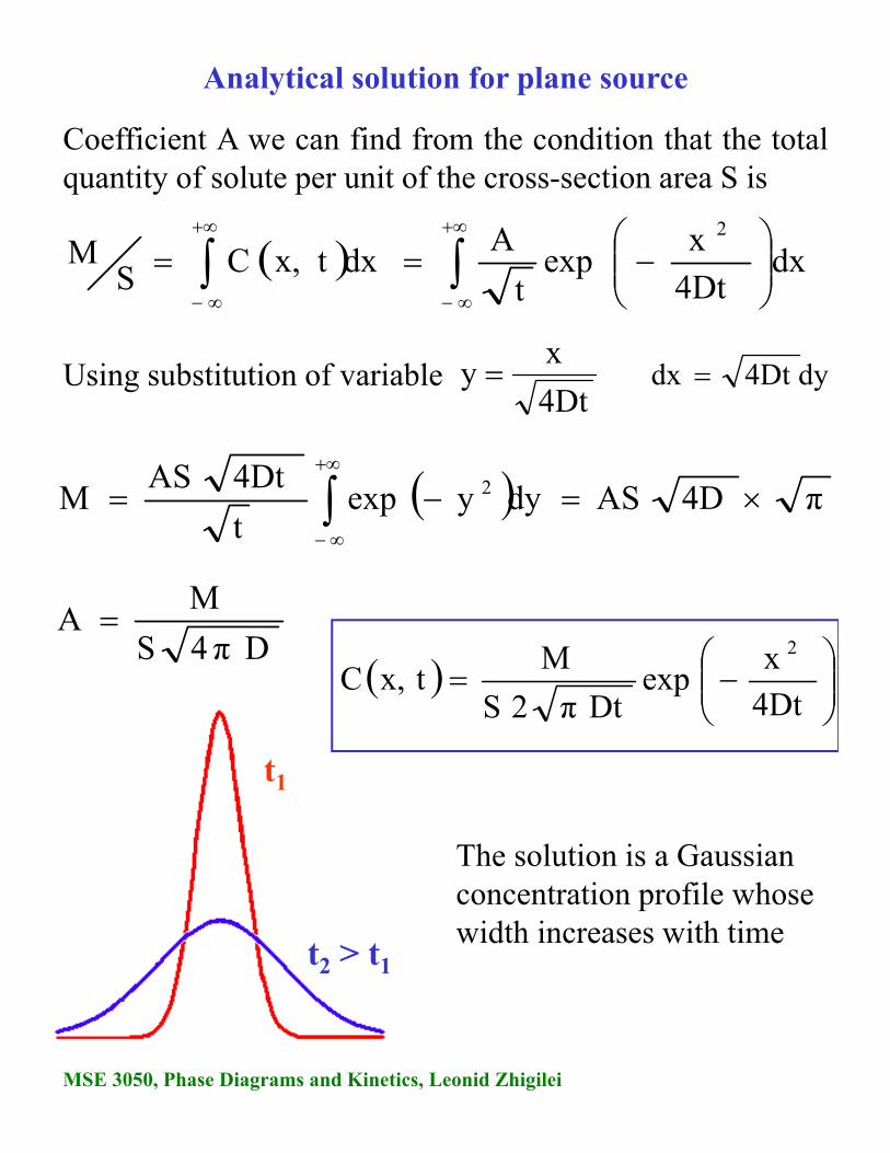
Coefficient A we can find from the condition that the totalquantity of solute per unit of the cross-section area S is
dx4Dt
xexp
t
Adxtx,CS
M2
Using substitution of variable4Dt
xy
π4DASdyyexpt
4DtASM 2
dy4Dtdx
D 4 πS
MA
4Dt
xexp
Dt π2 S
Mtx,C
2
The solution is a Gaussian concentration profile whose width increases with time
t1
t2 > t1
MSE 3050, Phase Diagrams and Kinetics, Leonid Zhigilei
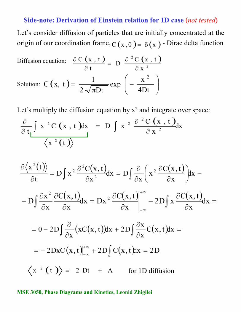
Side-note: Derivation of Einstein relation for 1D case (not tested)
Diffusion equation:
Let’s multiply the diffusion equation by x2 and integrate over space:
2
2
x
t,xCD
t
t,xC
dx
x
t,xCxDdxt,xCx
t 2
222
tx 2
dx
x
t,xCx
xDdx
x
t,xCxD
t
tx2
2
22
2
dxt,xCx
xD2dxt,xxC
xD20
dxx
t,xCxD2
x
t,xCDxdx
x
t,xC
x
xD 2
2
D2dxt,xCD2t,xDxC2
ADt2tx 2 for 1D diffusion
Let’s consider diffusion of particles that are initially concentrated at the
origin of our coordination frame, - Dirac delta function x0,xC
Solution:
4Dt
xexp
πDt2
1tx,C
2
MSE 3050, Phase Diagrams and Kinetics, Leonid Zhigilei
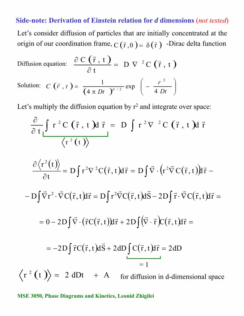
Side-note: Derivation of Einstein relation for d dimensions (not tested)
Diffusion equation:
Let’s multiply the diffusion equation by r2 and integrate over space:
t,rCDt
t,rC 2
rdt,rCrDrdt,rCrt
222
tr 2
rdt,rCrDrdt,rCrD
t
tr222
2
rdt,rCrD2rdt,rCrD20
rdt,rCrD2Sdt,rCrDrdt,rCrD 22
dD2rdt,rCdD2Sdt,rCrD2
AdDt2tr 2 for diffusion in d-dimensional space
= 1
Let’s consider diffusion of particles that are initially concentrated at the
origin of our coordination frame, -Dirac delta function r0,rC
Solution:
Dt
r
DttrC d 4
exp4
1,
2
2/
MSE 3050, Phase Diagrams and Kinetics, Leonid Zhigilei
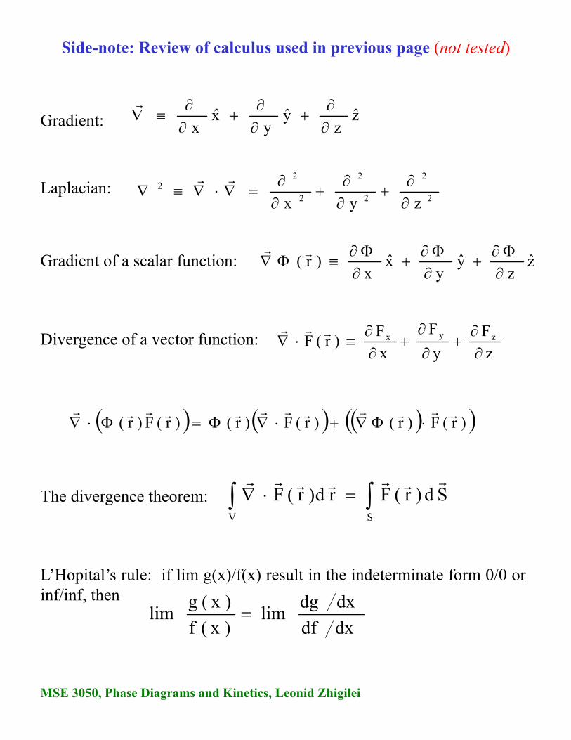
Side-note: Review of calculus used in previous page (not tested)
zz
yy
xx
Gradient:
Gradient of a scalar function: zz
yy
xx
)r(
Divergence of a vector function:z
F
y
F
x
F)r(F zyx
)r(F)r()r(F)r()r(F)r(
The divergence theorem: SV
Sd)r(Frd)r(F
2
2
2
2
2
22
zyx
Laplacian:
L’Hopital’s rule: if lim g(x)/f(x) result in the indeterminate form 0/0 orinf/inf, then
dxdf
dxdglim
)x(f
)x(glim

MSE 3050, Phase Diagrams and Kinetics, Leonid Zhigilei
Thin film deposited on a semi-infinite piece of material
Using the same solution we have a different condition for
coefficient A:dx
4Dt
xexp
t
ASM
0
2
Using substitution of variable4Dt
xy
2
π4DASdyyexp
t
4DtASM
0
2
dy4Dtdx
D πS
MA
4Dt
xexp
Dt πS
Mtx,C
2
The solution is a half of a Gaussian concentration profile. At the surface, the boundary condition
t1
t2 > t1
is satisfied 0x
C
0x
x0
0x
C
0x
MSE 3050, Phase Diagrams and Kinetics, Leonid Zhigilei
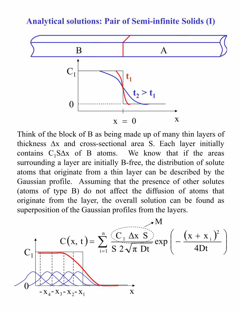
Analytical solutions: Pair of Semi-infinite Solids (I)
Think of the block of B as being made up of many thin layers ofthickness x and cross-sectional area S. Each layer initiallycontains C1Sx of B atoms. We know that if the areassurrounding a layer are initially B-free, the distribution of soluteatoms that originate from a thin layer can be described by theGaussian profile. Assuming that the presence of other solutes(atoms of type B) do not affect the diffusion of atoms thatoriginate from the layer, the overall solution can be found assuperposition of the Gaussian profiles from the layers.
A
C1
0t2 > t1
t1
B
0x x
x
C1
0
n
1i
2i1
4Dt
xxexp
Dt π2 S
SΔx Ctx,C
2x- 1x-4x- 3x-
M
MSE 3050, Phase Diagrams and Kinetics, Leonid Zhigilei
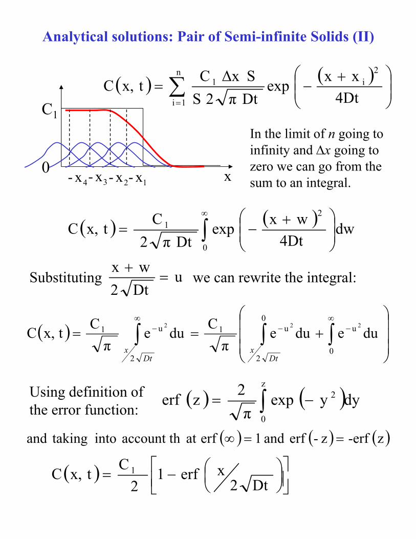
Analytical solutions: Pair of Semi-infinite Solids (II)
x
C1
0
n
1i
2i1
4Dt
xxexp
Dt π2 S
SΔx Ctx,C
0
21 dw
4Dt
wxexp
Dt π2
Ctx,C
In the limit of n going to infinity and x going to zero we can go from the sum to an integral.
Substituting uDt2
wx
we can rewrite the integral:
0
u0
2
u1
2
u1 duedue π
Cdue
π
Ctx,C
222
Dtx
Dtx
Using definition of the error function:
z-erfz-erf and 1erfat account th into takingand
z
0
2 dyyexpπ
2zerf
Dt2xerf1
2
Ctx,C 1
2x- 1x-4x- 3x-
MSE 3050, Phase Diagrams and Kinetics, Leonid Zhigilei
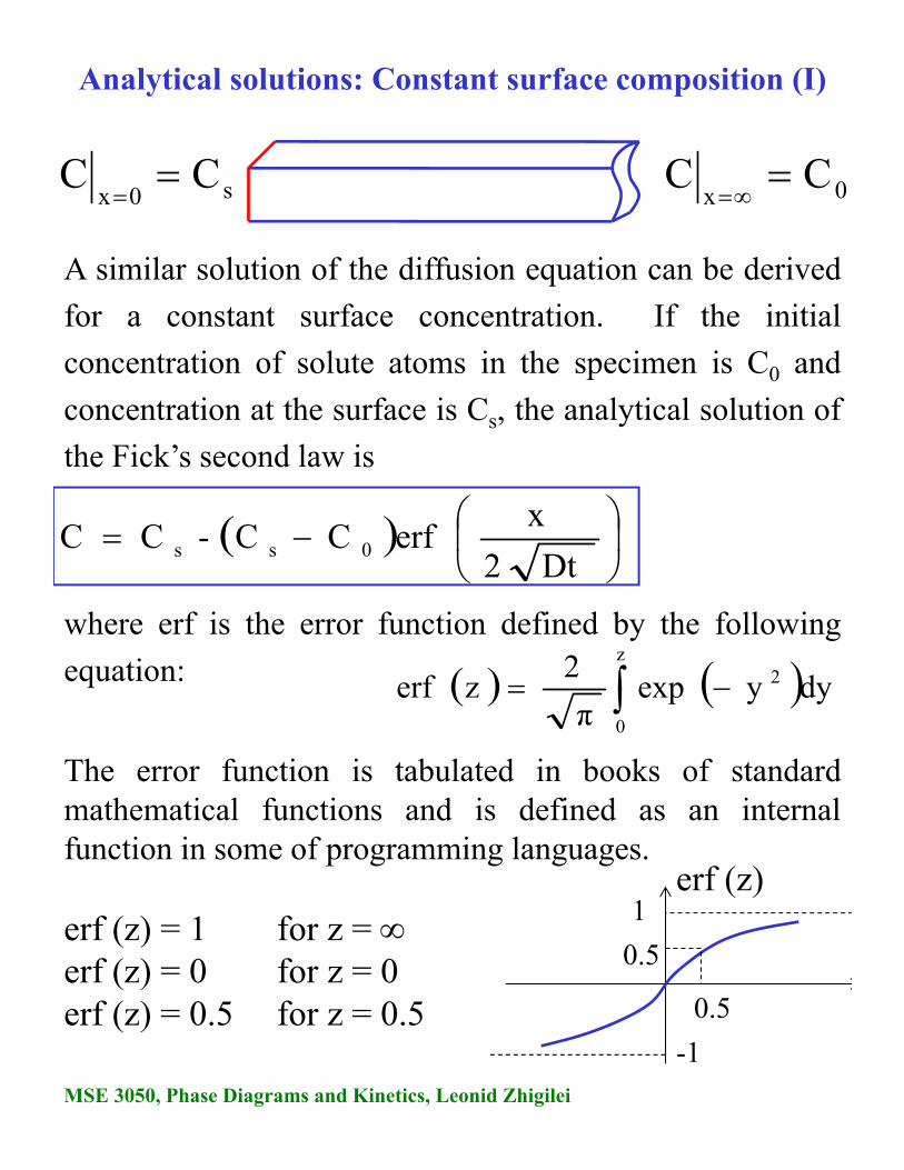
Analytical solutions: Constant surface composition (I)
A similar solution of the diffusion equation can be derived
for a constant surface concentration. If the initial
concentration of solute atoms in the specimen is C0 and
concentration at the surface is Cs, the analytical solution of
the Fick’s second law is
Dt2
xerfCC-CC 0ss
The error function is tabulated in books of standardmathematical functions and is defined as an internalfunction in some of programming languages.
erf (z) = 1 for z = erf (z) = 0 for z = 0erf (z) = 0.5 for z = 0.5
s0xCC
where erf is the error function defined by the following
equation: z
0
2 dyyexpπ
2zerf
0xCC
erf (z)1
-1
0.5
0.5

MSE 3050, Phase Diagrams and Kinetics, Leonid Zhigilei
Summary
Make sure you understand language and concepts:
Numerical integration of the diffusion equation (not tested)
Finite difference method
Spatial and time discretization
Initial and boundary conditions
Stability criterion
Analytical solutions for special cases
plane source
thin film on a semi-infinite substrate
diffusion pair
constant surface composition