finite-difference method for the hyperbolic system of equations with nonlocal boundary conditions

Ashyralyev and Prenov Advances in Difference Equations 2014, 2014:26http://www.advancesindifferenceequations.com/content/2014/1/26

RESEARCH Open Access

Finite-difference method for the hyperbolicsystem of equations with nonlocal boundaryconditionsAllaberen Ashyralyev1,2* and Rahat Prenov2

*Correspondence:[email protected] of Mathematics, FatihUniversity, Istanbul, Turkey2Department of Mathematics, ITTU,Ashgabat, Turkmenistan

AbstractIn the present paper, the finite-difference method for the initial-boundary valueproblem for a hyperbolic system of equations with nonlocal boundary conditions isstudied. The positivity of the difference analogy of the space operator generated bythis problem in the space C with maximum norm is established. The structure of theinterpolation spaces generated by this difference operator is investigated. Thepositivity of this difference operator in Hölder spaces is established. In applications,stability estimates for the solution of the difference scheme for a hyperbolic system ofequations with nonlocal boundary conditions are obtained. A numerical example isapplied.MSC: 35L40; 35L45

Keywords: hyperbolic system of equations; nonlocal boundary value problems;difference schemes; interpolation spaces; positivity of the difference operator; stabilityestimates

1 IntroductionNonlocal problems are widely used for mathematical modeling of various processes ofphysics, ecology, chemistry, and industry, when it is impossible to determine the bound-ary or initial values of the unknown function. The method of operators as a tool for theinvestigation of the solution of local and nonlocal problems for partial differential equa-tions in Hilbert and Banach spaces has been systematically developed by several authors(see, e.g., [–]). It is well known that (see, e.g., [–] and the references given therein)many application problems in fluid mechanics, physics, mathematical biology, and chem-istry were formulated as nonlocal mathematical models. Note that such problems werenot well studied in general.In the paper [], the initial-boundary value problem

⎧⎪⎪⎪⎨⎪⎪⎪⎩

∂u(t,x)∂t + a(x) ∂u(t,x)

∂x + δ(u(t,x) – v(t,x)) = f(t,x), < x < l, < t < T ,∂v(t,x)

∂t – a(x) ∂v(t,x)∂x + δv(t,x) = f(t,x), < x < l, < t < T ,

u(t, ) = γu(t, l), ≤ γ ≤ , βv(t, ) = v(t, l), ≤ β ≤ , ≤ t ≤ T ,u(,x) = u(x), v(,x) = v(x), ≤ x≤ l

()

©2014 Ashyralyev and Prenov; licensee Springer. This is an Open Access article distributed under the terms of the Creative Com-mons Attribution License (http://creativecommons.org/licenses/by/2.0), which permits unrestricted use, distribution, and repro-duction in any medium, provided the original work is properly cited.

http://www.advancesindifferenceequations.com/content/2014/1/26

mailto:[email protected]

http://creativecommons.org/licenses/by/2.0

Ashyralyev and Prenov Advances in Difference Equations 2014, 2014:26 of 24http://www.advancesindifferenceequations.com/content/2014/1/26

for the hyperbolic systemof equationswith nonlocal boundary conditionswas considered.Here

a(x)≥ a > , ()

u(x), v(x) (x ∈ [, l]), f(t,x), f(t,x) ((t,x) ∈ [,T]× [, l]) are given smooth functions andthey satisfy all compatibility conditions which guarantee the problem () has a smoothsolution u(t,x) and v(t,x). As noted in the paper [], the problem of sound waves []and the problem of the expansion of electricity oscillations [] can be replaced by theproblem (). Note that, we have the nonclassical initial-boundary value problem () withboundary conditions u(t, ) = γu(t, l), ≤ γ ≤ , βv(t, ) = v(t, l), ≤ β ≤ , ≤ t ≤ T .These conditions are given on two boundary points. It is clear that it is impossible todetermine the boundary values of the unknown function. So, these conditions are notlocal.Let E be a Banach space and A :D(A) ⊂ E → E be a linear unbounded operator densely

defined in E. We call A a positive operator in the Banach space if the operator (λI +A) hasa bounded inverse in E for any λ ≥ , and the following estimate holds:

∥∥(λI +A)–∥∥E→E ≤ M

λ + . ()

Throughout the present paper,M is defined as a positive constant. However, we will useM(α,β , . . .) to stress the fact that the constant depends only on α,β , . . . .For a positive operator A in the Banach space E, let us introduce the fractional spaces

Eα = Eα(E,A) ( < β < ) consisting of those v ∈ E for which the norm

‖v‖Eα = supλ>

λα∥∥A(λ +A)–v

∥∥E + ‖v‖E

is finite.Let us introduce the Banach space Cα[, l] = Cα([, l],R)×Cα([, l],R) (≤ α ≤ ) of all

continuous vector functions u =( u(x)u(x)

)defined on [, l] and satisfying a Hölder condition

for which the following norm is finite:

‖u‖Cα [,l] = ‖u‖C[,l]

+ supx,x+τ∈[,l]

τ �=

|u(x + τ ) – u(x)||τ |α + sup

x,x+τ∈[,l]τ �=

|u(x + τ ) – u(x)||τ |α .

Here C[, l] = C([, l],R)×C([, l],R) is the Banach space of all continuous vector func-tions u =

( u(x)u(x)

)defined on [, l] with norm

‖u‖C[,l] = maxx∈[,l]

∣∣u(x)∣∣ + maxx∈[,l]

∣∣u(x)∣∣.We consider the space operator A generated by the problem () defined by the formula

Au =(a(x) du(x)dx + δu(x) –δu(x)

–a(x) du(x)dx + δu(x)

)()



with domain

D(A) ={(

u(x)u(x)

): um(x),

dum(x)dx

∈ C([, l],R

),m = , ;

u() = γu(l),βu() = u(l)}.

The Green’s matrix function of A was constructed. The positivity of the operator A in theBanach space C[, l] was established. It was proved that for any α ∈ (, ) the norms inspaces Eα(C[, l],A) and

◦C

α[, l] are equivalent. The positivity of A in the Hölder spacesof

◦C

α[, l], α ∈ (, ) was proved. In applications, stability estimates for the solution of theproblem () for the hyperbolic system of equations with nonlocal boundary conditionswere obtained.In the present paper, the finite-difference method for the initial value problem for the

hyperbolic system of equations with nonlocal boundary conditions is applied. The pos-itivity of the difference analogy of the space operator A defined by equation () in thedifference analogy of C[, l] spaces is established. The structure interpolation spaces gen-erated by this difference operator is studied. The positivity of this difference operator inHölder spaces is established. In practice, stability estimates for the solution of the differ-ence scheme for the hyperbolic system of equations with nonlocal boundary conditionsare obtained. The method is illustrated by numerical example.The organization of the present paper as follows. Section is an introduction where

we provide the history and formulation of the problem. In Section , the Green’s matrixfunction of the difference space operator is presented and positivity of this operator inthe difference analogy of C[, l] spaces is proved. In Section , the structure of fractionalspaces generated by this difference operator is investigated and positivity of this differenceoperator in Hölder spaces is established. In Section , stable difference schemes for theapproximate solution of the problem () are constructed. A theorem on the stability forthe first order of accuracy in the t difference scheme is proved. In Section , a numericalapplication is given. Finally, Section is for our conclusion.

2 The Green’s matrix function of difference space operator and positivityLet us introduce the Banach spacesCα

h = Cαh ×Cα

h (≤ α ≤ ) andCh = Ch ×Ch of all meshvector functions uh =

{( u,nu,n–

)}Mn= defined on

[, l]h = {xn = nh, ≤ n≤M,Mh = l}

with the following norms:

∥∥uh∥∥C

αh=∥∥uh∥∥

Ch

+ sup≤n<n+m≤M

|u,n+m – u,n|(mh)α

+ sup≤k<k+m≤M–

|u,n+m – u,n|(mh)α

,

∥∥uh∥∥Ch

= max≤n≤M

|u,n| + max≤n≤M–

|u,n|.



We consider the difference space operator Axh generated by the problem () defined by the

formula

Axhuh =

(a(xn) u,n–u,n–h + δu,n –δu,n

–a(xn) u,n+–u,nh + δu,n

)()

acting on the space of mesh vector functions uh ={( u,n

u,n–)}M

n= defined on [, l]h, satisfyingthe conditions

u, = γu,M, βu, = u,M.

Here an = a(xn). We will study the resolvent of the difference space operator –Axh, i.e.

Axh

(uv

) h

+ λ

(uv

) h

=(

ϕ

ψ

) h

()

or⎧⎪⎨⎪⎩an un–un–

h + (δ + λ)un – δvn = ϕn, ≤ n≤M,–an+ vn+–vnh + (δ + λ)vn =ψn, ≤ n ≤M – ,u = γuM, βv = vM.

()

Lemma . For any λ ≥ , equation () is uniquely solvable and the following formulaholds:

(unvn

)=(Axh + λ

)–(ϕn

ψn

)=

M∑s=

G(n, s;λ)(

ϕs

ψs

)h

=(∑M

n=G(n, s;λ)ϕsh +∑M–

n= G(n, s;λ)ψsh∑M–n= G(n, s;λ)ψsh,

), ≤ n≤M, ()

where

G(n, s;λ) =(G(n, s;λ) G(n, s;λ)

G(n, s;λ)

).

Here

G(n, s;λ) =Q{U(n, s – ,λ)

as , ≤ s ≤ n,γU(n, ,λ)U(M, s – ,λ)

as , n + ≤ s ≤M,()

G(n, s;λ) = P{

β

as+U(M,n,λ)U(s + , ,λ), ≤ s ≤ n – ,

as+U(s + ,n,λ), n≤ s≤M – ,()

G(n, s;λ) = δ

M∑k=

G(n,k – ;λ)G(k, s;λ)h, ()

P =( – βU(M, ;λ)

)–, Q =( – γU(M, ;λ)

)–,



U(n,k;λ) ={Rn, . . . ,Rk+, n > k,, n = k,

Rn =( +

(δ + λ)han

)–, ≤ n≤M.

Proof Using the resolvent equation (), we get

–an+vn+ – vn

h+ (δ + λ)vn =ψn, ≤ n≤M – , βv = vM.

From that follows the following recursive formula:

vn = Rn+vn+ +h

an+Rn+ψn, ≤ n≤M – .

Hence

vn =U(M,n;λ)vM +M–∑s=n

U(s + ,n;λ) has+

ψs, ≤ n ≤M – .

From this formula and the nonlocal boundary condition βv = vM it follows that

vM = βPM–∑s=

U(s + , ;λ)h

as+ψs.

Then,

vn =U(M,n;λ)βPM–∑s=

U(s + , ;λ)h

as+ψs

+M–∑s=n

U(s + ,n;λ) has+

ψs = βPn–∑s=

U(M,n;λ)U(s + , ;λ)h

as+ψs

+ PM–∑s=n

U(s + ,n;λ) has+

ψs =M–∑s=

G(n, s;λ)ψsh. ()

Using the resolvent equation (), we get

anun – un–

h+ (δ + λ)un – δvn = ϕn, ≤ n≤M, u = γuM.

From that follows the system of recursion formulas

un = Rnun– +han

Rn(δvn + ϕn), ≤ n≤M.

Hence

un =U(n, ;λ)u +n∑k=

U(n,k – ;λ)hak

(δvk + ϕk), ≤ n≤M.



From this formula and the nonlocal boundary condition u = γuM it follows that

u = γQM∑k=

U(M,k – ;λ)hak

(δvk + ϕk).

Therefore,

un =U(n, ;λ)[γQ

M∑k=

U(M,k – ;λ)hak

(δvk + ϕk)]+

n∑k=

U(n,k – ;λ)hak

(δvk + ϕk)

=U(n, ;λ)γQM∑

s=n+U(M, s – ;λ)

has(δvs + ϕs) +

n∑s=

U(n, s – ;λ)has(δvs + ϕs)

=M∑s=

G(n, s – ;λ)ϕsh + δ

M∑s=

G(n, s – ;λ)vsh.

Applying equation (), we get

δ

M∑k=

G(n,k – ;λ)vkh = δ

M∑k=

G(n,k – ;λ)[M–∑

s=G(k, s;λ)ψsh

]h

=M–∑s=

[δ

M∑k=

G(n,k – ;λ)G(k, s;λ)h]ψsh

=M–∑s=

G(n, s;λ)ψsh.

From the last two formulas it follows that

un =M∑s=

G(n, s – ;λ)ϕsh +M–∑s=

G(n, s;λ)ψsh. ()

Lemma . is proved. �

Lemma . The following pointwise estimates hold; see equation ():

|P|, |Q| ≤ – rM

, ()

∣∣G(n, s;λ)∣∣≤

a( – rM)

{rn–s+, ≤ s≤ n,rM+n–s+, n + ≤ s≤ n≤M,

()

∣∣G(n, s;λ)∣∣≤

a( – rM)

{rM+s+–n, ≤ s ≤ n – ,rs+–n, n≤ s ≤M – ,

()

∣∣G(n, s;λ)∣∣≤

a( – rM)

{rn–s+, ≤ s≤ n,rs–n+, n + ≤ s ≤ n≤M – .

()

Here r = + (δ+λ)h

a.



Proof It is easy to see that the estimates of equations (), (), and () follow from thetriangle inequality. Applying the triangle inequality, we get

∣∣G(n, s;λ)∣∣≤ δ

s∑p=

∣∣G(n,p – ;λ)∣∣∣∣G(p, s;λ)

∣∣h. ()

If ≤ s ≤ n – . Then, using the estimates of equations (), (), (), and inequality (),we get

∣∣G(n, s;λ)∣∣≤ δ

s∑p=

∣∣G(n,p – ;λ)∣∣∣∣G(p, s;λ)

∣∣h

+ δ

n∑p=s+

∣∣G(n,p – ;λ)∣∣∣∣G(p, s;λ)

∣∣h

+ δ

M∑p=n+

∣∣G(n,p – ;λ)∣∣∣∣G(p, s;λ)

∣∣h

≤ δ

a( – rM)

[ s∑p=

rn–p+rs+–ph +n∑

p=s+rn–p+rM+s+–ph

+M∑

p=n+rM+n–p+rM+s+–ph

]

=δrn–s+

a( – rM)

[ s∑p=

rs–ph +n∑

p=s+rM+s–ph +

M∑p=n+

rM+s–ph]

=δhrn–s+

a( – rM)( – r)[ – rs +

( – r(n–s)

)rM+s–n + rs

( – r(M–n))]

=δhrn–s+( – rM)a( – rM)( – r)

[ + rM+s–n]

=δhrn–s+( – rM)a( – rM)( – r)

[ + rM+s–n]

=δhrn–s+( – rM)

a( – rM)r δ+λa h( + r)

[ + rM+s–n]≤ rn–s+

a( – rM).

If s = n. Then, using the estimates of equations (), (), (), and inequality (), we get

∣∣G(n, s;λ)∣∣≤ δ

n∑p=

∣∣G(n,p – ;λ)∣∣∣∣G(p, s;λ)

∣∣h

+ δ

M∑p=n+

∣∣G(n,p – ;λ)∣∣∣∣G(p, s;λ)

∣∣h

≤ δ

a( – rM)

[ n∑p=

rn–p+rs+–ph +M∑

p=n+rM+n–p+rM+s+–ph

]

=δr

a( – rM)

[ n∑p=

rs–ph +M∑

p=n+rM+s–ph

]



=δhr

a( – rM)( – r)[ – rn +

( – r(M–s))rs]

=δhr( – rM)

a( – rM)( – r)=

δhr( – rM)a( – rM)r δ+λ

a h( + r)≤ r

a( – rM).

Here n≤ s≤M. Then, using the estimates of equations (), (), (), and inequality (),we get

∣∣G(n, s;λ)∣∣≤ δ

n∑p=

∣∣G(n,p – ;λ)∣∣∣∣G(p, s;λ)

∣∣h

+ δ

s∑p=n+

∣∣G(n,p – ;λ)∣∣∣∣G(p, s;λ)

∣∣h

+ δ

M∑p=s+

∣∣G(n,p – ;λ)∣∣∣∣G(p, s;λ)

∣∣h

≤ δ

a( – rM)

[ n∑p=

rn–p+rs+–ph +s∑

p=n+rs+–prM+n–ph

+M∑

p=s+rs+–prM+n–ph

]

=δrs–n+

a( – rM)

[ n∑p=

rn–ph +s∑

p=n+rM+n–ph +

M∑p=s+

rM+n–ph]

=δhrs–n+

a( – rM)( – r)[ – rn +

( – r(n–s)

)rM+s–n + rn

( – r(M–s))]

=δhrs–n+( – rM)a( – rM)( – r)

[ + rM+s–n]

=δhrs–n+( – rM)a( – rM)( – r)

[ + rM+s–n]

=δhrs–n+

a( – rM)r δ+λa h( + r)

[ + rM+s–n]≤ rs–n+

a( – rM).

Lemma . is proved. �

Theorem . The operator (λI + Axh) has a bounded inverse in Ch for any λ ≥ and the

following estimate holds:

∥∥(λ +Axh)–∥∥

Ch→Ch≤ M

+ λ. ()

Proof Using the formula equation () and the triangle inequality, we get

|un| ≤M∑k=

h∣∣G(n,k – ;λ)

∣∣ max≤k≤M

|ϕk| +M–∑k=

h∣∣G(n,k;λ)

∣∣ max≤k≤M–

|ψk|

≤[ M∑

k=h∣∣G(n,k – ;λ)

∣∣ + M–∑k=

h∣∣G(n,k;λ)

∣∣]∥∥∥∥∥(

ϕ

ψ

) h∥∥∥∥∥Ch[,l]

,



|vn| ≤M–∑k=

h∣∣G(n,k;λ)

∣∣ max≤k≤M–

|ψk|

≤M–∑k=

h∣∣G(n,k;λ)

∣∣∥∥∥∥∥(

ϕ

ψ

) h∥∥∥∥∥Ch[,l]

,

for any n = , , . . . ,M. Using the estimate of equation (), we get

M∑k=

h∣∣G(n,k – ;λ)

∣∣≤ ra( – rM)

[ n∑k=

rn–kh +M∑

k=n+rM+n–kh

]

=hr

a( – rM)r δ+λa h[ – rn + rn

( – rM–n)] =

δ + λ.

Using the estimate of equation (), we get

M–∑k=

h∣∣G(n,k;λ)

∣∣≤ a( – rM)

[ n–∑k=

rM+k+–nh +M–∑k=n

rk+–nh]

=hr

a( – rM)r δ+λa h[ – rM–n + rM–n( – rn

)]=

δ + λ

.

Using the estimate of equation (), we get

M–∑k=

h∣∣G(n,k;λ)

∣∣≤ ra( – rM)

[ n∑k=

rn–kh +M–∑k=n+

rk–nh]

=hr

a( – rM)r δ+λa h[ – rn+ + r

( – rM–n–)]≤

δ + λ.

Therefore,

max≤n≤M

|un| ≤[ M∑

k=h∣∣G(n,k – ;λ)

∣∣ + M–∑k=

h∣∣G(n,k;λ)

∣∣]∥∥∥∥∥(

ϕ

ψ

) h∥∥∥∥∥Ch[,l]

≤ δ + λ

∥∥∥∥∥(

ϕ

ψ

) h∥∥∥∥∥Ch[,l]

,

max≤n≤M–

|vn| ≤M–∑k=

h∣∣G(n,k;λ)

∣∣∥∥∥∥∥(

ϕ

ψ

) h∥∥∥∥∥Ch[,l]

≤ δ + λ

∥∥∥∥∥(

ϕ

ψ

) h∥∥∥∥∥Ch[,l]

.

From this it follows that

∥∥∥∥∥(uv

) h∥∥∥∥∥Ch[,l]

≤ δ + λ

∥∥∥∥∥(

ϕ

ψ

) h∥∥∥∥∥Ch[,l]

.

Theorem . is proved. �



3 The structure of fractional spaces Eα(Ch,Axh) and positivity of Ax

h in Hölderspaces

Clearly, the operator Axh and its resolvent (Ax

h + λ)– commute. By the definition of thenorm in the fractional space Eα = Eα(Ch,Ax

h), we get∥∥(Axh + λ

)–∥∥Eα→Eα

≤ ∥∥(Axh + λ

)–∥∥Ch→Ch

.

Thus, from Theorem . it follows that Axh is a positive operator in the fractional spaces

Eα(Ch,Axh). Moreover, we have the following result.

Theorem . For α ∈ (, ), the norms of the spaces Eα(Ch,Axh) and the Hölder space

◦C

αh

are equivalent uniformly with respect to h. Here

◦C

αh ={(

ϕ

ψ

) h

∈ Cαh :

ϕ = γ ϕM, ≤ γ ≤ ,βψ =ψM, ≤ β ≤ }. ()

Proof For any λ ≥ we have the obvious equality

Axh(Axh + λ

)–(ϕn

ψn

)=(

ϕn

ψn

)– λ(Axh + λ

)–(ϕn

ψn

).

By equation (), we can write

Axh(Axh + λ

)–(ϕn

ψn

)

=(

ϕn

ψn

)– λ

M∑k=

G(n,k;λ)h(

ϕn

ψn

)

=([ – λ

∑nk=G(n,k;λ)h]ϕn – λ

∑Mk=n+G(n,k;λ)hϕM

)

+(

–λ∑M–

k= G(n,k;λ)hψn

–λ∑n–

k=G(n,k;λ)hψ + [ – λ∑M–

k=n G(n,k;λ)h]ψn

)

+(

λ∑n

k=G(n,k;λ)(ϕn – ϕk)h + λ∑M

k=n+G(n,k;λ)(ϕM – ϕk)h

)

+(

λ∑M–

k= G(n,k;λ)(ψn –ψk)hλ∑n–

k=G(n,k;λ)(ψ –ψk)h + λ∑M–

k=n G(n,k;λ)(ψn –ψk)h

). ()

Applying equation () and the following obvious equalities:

– λ

n∑k=

G(n,k;λ)h = –Qλ

n∑k=

U(n, s – ;λ)has

= –Qλ

δ + λ

n∑k=

(U(n, s – ;λ) –U(n, s;λ)

)



= –Qλ

δ + λ

( –U(n, ;λ)

)=

δ

δ + λQ – γQU(M, ;λ) +

λ

δ + λQU(n, ;λ),

–λ

M∑k=n+

G(n,k;λ) = –Qλ

M∑k=n+

γ

asU(n, s – ;λ)U(M, ;λ)

= –λ

δ + λQ

M∑k=n+

γU(M, ;λ)(U(n, s – ;λ) –U(n, s;λ)

)

= –λ

δ + λγQU(M, ;λ)

(U(n, ;λ) –U(n,M;λ)

)= –

λ

δ + λγQ[U(M, ;λ)U(n, ;λ) –U(n, ;λ)

],

– λ

M–∑s=n

G(n,k;λ)h = – Pλ

M–∑s=n

as+

U(s + ,n;λ)h

= – Pλ

δ + λ

M–∑s=n

[U(s,n;λ) –U(s + ,n;λ)

]h

= – P λ

δ + λ

[ –U(M,n;λ)

]h

= P δ

δ + λ– PβU(M, ;λ) + P λ

δ + λU(M,n;λ),

–λ

n–∑s=

G(n,k;λ)h = –Pλ

n–∑s=

β

as+U(M,n;λ)U(s + , ;λ)h

– λβ

n–∑s=

PU(M,n;λ) δ + λ

[U(s,n;λ) –U(s + ,n;λ)

]h

– λβP δ + λ

U(M,n;λ)[U(,n;λ) –

]h,

–λ

M–∑s=

G(n, s;λ)h = –λ

M–∑s=

δhM∑k=

G(n,k – ;λ)G(k, s;λ)h

= –λ

M∑k=

[ k–∑s=

δhG(n,k – ;λ)G(k, s;λ)h

+M–∑s=k

δhG(n,k – ;λ)G(k, s;λ)h]

= –λ

n+∑k=

k–∑s=


– λ

M∑k=n+

k–∑s=


= –λ

n+∑k=

M–∑s=k




– λ

M∑k=n+

M–∑s=k


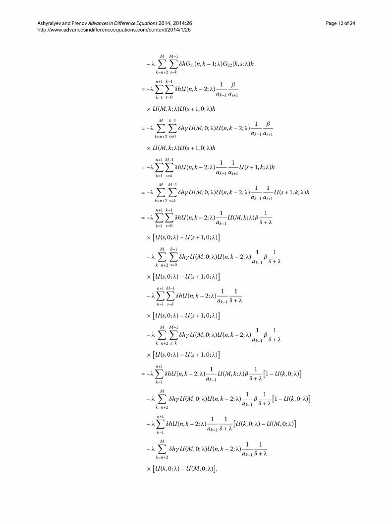
= –λ

n+∑k=

k–∑s=

δhU(n,k – ;λ)

ak–β

as+

×U(M,k;λ)U(s + , ;λ)h

= –λ

M∑k=n+

k–∑s=

δhγU(M, ;λ)U(n,k – ;λ)

ak–β

as+

×U(M,k;λ)U(s + , ;λ)h

= –λ

n+∑k=

M–∑s=k

δhU(n,k – ;λ)

ak–

as+U(s + ,k;λ)h

= –λ

M∑k=n+

M–∑s=k


ak–

as+U(s + ,k;λ)h

= –λ

n+∑k=

k–∑s=

δhU(n,k – ;λ)

ak–U(M,k;λ)β

δ + λ

× [U(s, ;λ) –U(s + , ;λ)]

– λ

M∑k=n+

k–∑s=


ak–β

δ + λ

× [U(s, ;λ) –U(s + , ;λ)]

– λ

n+∑k=

M–∑s=k

δhU(n,k – ;λ)

ak–

δ + λ

× [U(s, ;λ) –U(s + , ;λ)]

– λ

M∑k=n+

M–∑s=k


ak–β

δ + λ

× [U(s, ;λ) –U(s + , ;λ)]

= –λ

n+∑k=

δhU(n,k – ;λ)

ak–U(M,k;λ)β

δ + λ

[ –U(k, ;λ)

]

– λ

M∑k=n+


ak–β

δ + λ

[ –U(k, ;λ)

]

– λ

n+∑k=

δhU(n,k – ;λ)

ak–

δ + λ

[U(k, ;λ) –U(M, ;λ)

]

– λ

M∑k=n+


ak–

δ + λ

× [U(k, ;λ) –U(M, ;λ)],



and using the nonlocal boundary conditions

ϕ = γ ϕM, βψ =ψM,

we get

Axh(λ +Ax

h)–(ϕn

ψn

)

=([ δδ+λ

Q – γQU(M, ;λ)]ϕn +Q λδ+λ

U(n, ;λ)(ϕn – ϕ)

)

=(

λδ+λ

γQU(M, ;λ)U(n, ;λ)ϕM

–λβPU(M,n;λ) δ+λ

U(,n;λ)ψ

)

+(

{–λ∑n+

k= δhU(n,k – ;λ) ak–

U(M,k;λ)β δ+λ

[ –U(k, ;λ)]}ψn

[P δδ+λ

– PβU(M, ;λ)]ψn + P λδ+λ

U(M,n;λ)(ψn –ψM)

)

+(–λ∑n+


U(M,k;λ)β δ+λ

[ –U(k, ;λ)]ψn

)

+(–λ∑M

k=n+ δhγU(M, ;λ)U(n,k – ;λ) ak–

β δ+λ

[ –U(k, ;λ)]ψn

)

+(–λ∑n+


δ+λ

[U(k, ;λ) –U(M, ;λ)]ψn

)

+(–λ∑M

k=n+ δhγU(M, ;λ)U(n,k – ;λ) ak–

β δ+λ

[U(k, ;λ) –U(M, ;λ)]ψn

)

+(

λ∑n+

k=G(n,k;λ)(ϕn – ϕk)h + λ∑M

k=n+G(n,k;λ)(ϕM – ϕk)h

)

+(

λ∑M–

k= G(n,k;λ)(ψn –ψk)hλ∑n–

k=G(n,k;λ)(ψ –ψk)h + λ∑M–

k=n G(n,k;λ)(ψn –ψk)h

).

Using this formula, the triangle inequality and the definition of spaces Eα(C[, l]h,Axh)

and Cα[, l]h, we get

∥∥∥∥∥λαAxh(Axh + λ

)– (ϕ

ψ

) h∥∥∥∥∥C[,l]h

≤ max≤n≤M

[λαδ

δ + λ|Q| + γ |Q|λα

∣∣U(M, ;λ)∣∣ + λ+α

δ + λγ |Q|∣∣U(M, ;λ)

∣∣∣∣U(n, ;λ)∣∣]

× max≤n≤M

|ψn|

+ max≤n≤M

λ+α

δ + λ|Q|(nh)α∣∣U(n, ;λ)

∣∣ sup≤n≤M

|ϕn – ϕ|(nh)α

+ max≤n≤M

[λαδ

δ + λ|P| + β|P|λα

∣∣U(M, ;λ)∣∣ + λ+α

δ + λβ|P|∣∣U(M,n;λ)

∣∣∣∣U(,n;λ)∣∣]



× max≤n≤M

|ψn| + max≤n≤M

λ+α

δ + λ|P|((M – n)h

)α∣∣U(M,n;λ)∣∣

× sup≤n≤M–

|ψn –ψM|((M – n)h)α

+ max≤n≤M

λ+α

n+∑k=

δh∣∣U(n,k – ;λ)

∣∣ ak–

∣∣U(M,k;λ)∣∣

× β

δ + λ

∣∣ –U(k, ;λ)∣∣ max≤n≤M

|ψn|

+ max≤n≤M

λ+α

M∑k=n+

δhγ∣∣U(M, ;λ)

∣∣∣∣U(n,k – ;λ)∣∣ ak–

β

δ + λ

∣∣ –U(k, ;λ)∣∣

× max≤n≤M

|ψn|

+ max≤n≤M

λ+α

n+∑k=


∣∣ ak–

δ + λ

∣∣U(k, ;λ) –U(M,k;λ)∣∣ max≤n≤M

|ψn|

+ max≤n≤M

λ+α

M∑k=n+


∣∣∣∣U(n,k – ;λ)∣∣ ak–

× δ + λ

∣∣U(k, ;λ) –U(M, ;λ)∣∣ max≤n≤M

|ψn|

+ max≤n≤M

λ+α

n+∑k=

((n – k)h

)α∣∣G(n,k;λ)∣∣h sup

≤k≤n≤M

|ϕn – ϕk|((n – k)h)α

+ max≤n≤M

λ+α

M∑k=n+

((M – n)h


≤n≤M–

|ϕM – ϕk|((M – n)h)α

+ max≤n≤M

λ+α

M–∑k=

(|k – n|h)α∣∣G(n,k;λ)∣∣h sup

≤k,n≤M,k �=n

|ψn –ψk|(|n – k|h)α

+ max≤n≤M

λ+α

n–∑k=

(kh)α∣∣G(n,k;λ)

∣∣h sup≤k≤M

|ψk –ψ|(kh)α

+ max≤n≤M

λ+α

M–∑k=n+

((k – n)h


≤n≤k≤M–

|ψn –ψk|((k – n)h)α

≤ J∥∥∥∥∥(

ϕ

ψ

) h∥∥∥∥∥C

αh

.

Here

J =λαδ

δ + λ|Q| + γ |Q|λα

∣∣U(M, ;λ)∣∣

+ max≤n≤M

{λ+α

δ + λγ |Q|∣∣U(M, ;λ)

∣∣∣∣U(n, ;λ)∣∣ + λ+α

δ + λ|Q|(nh)α∣∣U(n, ;λ)

∣∣× λαδ

δ + λ|P| + β|P|λα

∣∣U(M, ;λ)∣∣ + λ+α

δ + λβ|P|∣∣U(M,n;λ)

∣∣∣∣U(,n;λ)∣∣



+λ+α

δ + λ|P|((M – n)τ

)α∣∣U(M,n;λ)∣∣

+ λ+α

n+∑k=


∣∣ ak–

∣∣U(M,k;λ)∣∣β

δ + λ

∣∣ –U(k, ;λ)∣∣

+ λ+α

M∑k=n+


∣∣∣∣U(n,k – ;λ)∣∣ ak–

β

δ + λ

∣∣ –U(k, ;λ)∣∣

+ λ+α

n+∑k=


∣∣ ak–

δ + λ

∣∣U(k, ;λ) –U(M,k;λ)∣∣ + λ+α

×M∑

k=n+δhγ

∣∣U(M, ;λ)∣∣∣∣U(n,k – ;λ)

∣∣ ak–

δ + λ

∣∣U(k, ;λ) –U(M, ;λ)∣∣

+ λ+α

n+∑k=

((n – k)τ

)α∣∣G(n,k;λ)∣∣h + λ+α

M∑k=n+

((M – n)τ

)α∣∣G(n,k;λ)∣∣h

+ λ+α

M–∑k=

(|k – n|τ)α∣∣G(n,k;λ)∣∣h + λ+α

n–∑k=

(kτ )α∣∣G(n,k;λ)

∣∣h

+ λ+α

M–∑k=n+

((k – n)τ

)α∣∣G(n,k;λ)∣∣h}.

Using the estimates

λαδ–α

δ + λ≤ ,

λ+αδ–α

(δ + λ)≤ ,

and the estimates of equations (), (), (), and (), we get

J ≤ max≤n≤M

{λαδ

δ + λ

– rM

+

– rMλα

( +

(δ + λ)ha

)–M

+λ+α

δ + λ

– rM

( +

(δ + λ)ha

)–M–n++

λ+α

δ + λ

– rM

(nτ )α( +

(δ + λ)ha

)–n

+λαδ

δ + λ

– rM

+

– rMλα

( +

(δ + λ)ha

)–M+

λ+α

δ + λ

– rM

( +

(δ + λ)ha

)–M

+λ+α

δ + λ

– rM

((M – n)h

)α( + (δ + λ)ha

)–M+n

+ λ+α

n+∑k=

δhrn–k++M–k a

δ + λ

+ λ+α

M∑k=n+

δhrM+n–k+ a

δ + λ

+ λ+α

n+∑k=

δhrn–k+a

δ + λ

+ λ+α

M∑k=n+

δhrM+n–k+ a

δ + λ

+ λ+α

n+∑k=

((n – k)h

)αrn–k+ ah + λ+α

M∑k=n+

((M – k)h

)αrM–k+ ah



+ λ+α

M–∑k=

(|k – n|h)αr|n–k|+ ah + λ+α

n–∑k=

(kh)αrk+ ah

+ λ+α

M–∑k=n+

((k – n)h

)αrk–n+ ah}

≤M(a, δ).

Then

∥∥∥∥∥λαAxh(Axh + λ

)– (ϕ

ψ

) h∥∥∥∥∥Ch

≤M(a, δ)∥∥∥∥∥(

ϕ

ψ

) h∥∥∥∥∥C

αh

for any λ ≥ . This means that

∥∥∥∥∥(

ϕ

ψ

) h∥∥∥∥∥Eα (Ch ,Ax

h)

≤M(a, δ)∥∥∥∥∥(

ϕ

ψ

) h∥∥∥∥∥C

αh

.

Let us prove the opposite inequality. For any positive operator Axh we can write

(fg

)=∫ ∞

Axh(λ +Ax

h)–(f

g

)dλ.

From the relation and formula () it follows that

(ϕn

ψn

)=∫ ∞

(λ +Ax

h)–Ax

h(λ +Ax

h)–(ϕn

ψn

)dλ

=∫ ∞

M∑k=

G(n,k;λ)hAxh(λ +Ax

h)–(ϕk

ψk

)dλ

=∫ ∞

M∑s=

G(n, s;λ)hAxh(λ +Ax

h)–(ϕs

)dλ

+∫ ∞

M–∑s=


h)–(

ψs

)dλ

+∫ ∞

M–∑s=


h)–(

ψs

)dλ.

Consequently,

(ϕn+m

ψn+m

)=(

ϕn

ψn

)

=∫ ∞

M–∑k=

(G(n +m,k;λ) –G(n,k;λ)

)hAx

h(λ +Ax

h)–(ϕk

ψk

)dλ,



whence

|ϕn+m – ϕn| ≤∫ ∞

M∑s=

λ–α∣∣G(n +m, s;λ) –G(n, s;λ)

∣∣hdλ

∥∥∥∥∥(

ϕ

ψ

) h∥∥∥∥∥Eα (Ch ,Ax

h)

+∫ ∞

M–∑s=

λ–α∣∣G(n +m, s;λ) –G(n, s;λ)

∣∣hdλ

∥∥∥∥∥(

ϕ

ψ

) h∥∥∥∥∥Eα (Ch ,Ax

h)

,

|ψn+m –ψn| ≤∫ ∞

M–∑s=

λ–α∣∣G(n +m, s;λ) –G(n, s;λ)

∣∣hdλ

∥∥∥∥∥(

ϕ

ψ

) h∥∥∥∥∥Eα (Ch ,Ax

h)

.

Let

P = (mh)–α

∫ ∞

M∑s=

λ–α∣∣G(n +m, s;λ) –G(n, s;λ)

∣∣hdλ

+ (mh)–α

∫ ∞

M–∑s=

λ–α∣∣G(n +m, s;λ) –G(n, s;λ)

∣∣hdλ

+ (mh)–α

∫ ∞

M–∑s=

λ–α∣∣G(n +m, s;λ) –G(n, s;λ)

∣∣hdλ.

Then for any n +m,n ∈ {, , . . . ,M}, we have

(mh)–α|ϕn+m – ϕn| + (mh)–α|ψn+m –ψn| ≤ P∥∥∥∥∥(

ϕ

ψ

) h∥∥∥∥∥Eα (C[,l]h ,Ax

h)

.

Now let us estimate P = P + P + P, where

P = (mh)–α

∫ ∞

M∑s=

λ–α∣∣G(n +m, s;λ) –G(n, s;λ)

∣∣hdλ,

P = (mh)–α

∫ ∞

M–∑s=

λ–α∣∣G(n +m, s;λ) –G(n, s;λ)

∣∣hdλ,

P = (mh)–α

∫ ∞

M–∑s=

λ–α∣∣G(n +m, s;λ) –G(n, s;λ)

∣∣hdλ.

Note that it suffices to consider the case when ≤ mh ≤ . Applying the scheme of the

paper [] and using equations (), (), (), (), and the estimates of equations (), (),(), and (), we can establish the following estimate:

Pr ≤ M(a, δ)α( – α)

()

for r = , , . Applying the triangle inequality and the estimate of equation (), we get

P ≤ M(a, δ)α( – α)

.



Thus for any n +m,n ∈ {, , . . . ,M} we have

|mh|–α|ϕn+m – ϕn| + |mh|–α|ψn+m –ψn| ≤ M(a, δ)α( – α)

∥∥∥∥∥(

ϕ

ψ

) h∥∥∥∥∥Eα (Ch ,Ah)

.

This means that the following inequality holds:

∥∥∥∥∥(

ϕ

ψ

) h∥∥∥∥∥Cαh

≤ M(a, δ)α( – α)

∥∥∥∥∥(

ϕ

ψ

) h∥∥∥∥∥Eα (Ch ,Ah)

.

Theorem . is proved. �

Since the Axh is a positive operator in the fractional spaces Eα(Ch,Ax

h), from the result ofTheorem . it follows that it is also a positive operator in the Hölder space

◦C

αh . Namely,

we have the following.

Theorem . The operator (λI +Axh) has a bounded inverse in

◦C

αh uniformly with respect

to h for any λ ≥ and the following estimate holds:

∥∥(λI +Axh)–∥∥ ◦

Cαh→◦

Cαh

≤ M(a, δ)α( – α)

M

+ λ.

4 ApplicationsIn this section we consider the application of results of Sections and . For a positiveoperator A in E the following result was established in papers [, ].

Theorem . Let A be a positive operator in E. Then it obeys the following estimate:

∥∥Rkq,q–(τA)

∥∥E→E ≤M, ≤ k ≤N ,Nτ = T , ()

where M does not depend on τ and k.Here Rq,q–(z) is the Padé approximation of exp(–z)near z = .

For a numerical solution of the initial-boundary value problem () the following differ-ence scheme is presented:

⎧⎪⎪⎪⎪⎪⎪⎪⎪⎪⎪⎪⎨⎪⎪⎪⎪⎪⎪⎪⎪⎪⎪⎪⎩

ukn–uk–nτ

+ a(xn)ukn–ukn–

h + δ(ukn – vkn) = f k,n, f k,n = f(tk ,xn),tk = kτ ,xn = nh, ≤ k ≤N ,Nτ = T , ≤ n≤M,Mh = l,

vkn–vk–nτ

– a(xn+)vkn+–v

kn

h + δvkn = f k,n, f k,n = f(tk ,xn),tk = kτ ,xn = nh, ≤ k ≤N ,Nτ = T , ≤ n ≤M – ,Mh = l,

uk = γukM, ≤ γ ≤ , βvk = vkM, ≤ β ≤ , ≤ k ≤N ,un = u(xn), vn = v(xn), xn = nh, ≤ n≤M,Mh = l.

()

We introduce the Banach space C([,T]τ ,E) of all continuous abstract mesh vector func-tions

uτ ={uk}Nk= =

{(uk,nuk,n

) h}N

k=



defined on [,T]τ = {tk = kτ , ≤ k ≤N ,Nτ = T}with values in E, equipped with the norm

∥∥uτ∥∥C([,T]τ ,E) = max

≤k≤N

∥∥{uk,n}Mn=∥∥E + max≤k≤N

∥∥{uk,n}Mn=∥∥E .Note that the problem () can be written in the form of the abstract Cauchy problem

{(uk–uk–

τvk–vk–

τ

) h}N

k=

+Axh

{(uk

vk

) h}N

k=

={(

f kf

) h}N

k=

, ≤ k ≤N ,

(uv

)=(unvn–

)M

n=

()

in a Banach space E = Ch with a positive operator Axh defined by (). Here

{( f kf k

)h}Nk= ={( f k,n

f k,n–

)Mn=}Nk= is the given abstract vector function defined on [,T]τ with values in E,( u

v)=( unvn–

)Mn= is the element of D(Ax

h). It is well known that (see, for example []) theformula

(uk

vk

)=(I + τAx

h)–k (u

v

)+

k∑j=

(I + τAx

h)–k+j–(f j

f j

)τ ()

gives a solution of the problem () in C([,T]τ ,E).

Theorem . For the solution of the problem () the stability inequality holds:

∥∥∥∥∥{(

uk

vk

)}N

k=

∥∥∥∥∥C([,T]τ ,E)

≤M(a, δ)[∥∥∥∥∥(uv

)∥∥∥∥∥E

+

∥∥∥∥∥{(

f kf k

)}N

k=

∥∥∥∥∥C([,T]τ ,E)

].

The proof of Theorem . is based on the positivity of the operator Axh, equation ()

and the estimate of equation ().Applying the results of Theorems . and ., we get the following theorem.

Theorem . The solution of the problem () satisfies the following estimate:

max≤k≤N

max≤n≤M

∣∣ukn∣∣ + max≤k≤N

max≤n≤M–

∣∣vkn∣∣≤M(a, δ)

[max≤n≤M

∣∣un∣∣ + max≤n≤M–

∣∣vn∣∣ + max≤k≤N

max≤n≤M

∣∣f k,n∣∣ + max≤k≤N

max≤n≤M–

∣∣f k,n∣∣].Applying results of Theorems ., ., and ., we get the following theorem.

Theorem . Assume that

f k, = γ f k,M, ≤ γ ≤ ,

βf k, = f k,M, ≤ β ≤ , ≤ k ≤N .



Then the solution of the problem () satisfies the following estimate:

max≤k≤N

(max≤n≤M

∣∣ukn∣∣ + sup≤n<n+m≤N

|ukn+m – ukn|(mτ )α

)

+ max≤k≤N

(max

≤n≤M–

∣∣vkn∣∣ + sup≤n<n+m≤M–

|vkn+m – vkn|(mτ )α

)

≤M(a, δ,α)[

max≤n≤M

∣∣un∣∣ + sup≤n<n+m≤N

|un+m – un|(mτ )α

+ max≤n≤M–

∣∣vn∣∣ + sup≤n<n+m≤M–

|vn+m – vn|(mτ )α

+ max≤k≤N

(max≤n≤M

∣∣f k,n∣∣ + sup≤n<n+m≤N

|f k,n+m – f k,n|(mτ )α

)

+ max≤k≤N

(max

≤n≤M–

∣∣f k,n∣∣ + sup≤n<n+m≤M–

|f k,n+m – f k,n|(mτ )α

)].

Finally, one has not been able to obtain a sharp estimate for the constants figuring inthe stability estimates. Therefore, our interest in the present paper is studying the differ-ence scheme equation () by numerical experiments. Applying this difference scheme,the numerical method is proposed in the following section for the numerical solution ofthe hyperbolic system of equations with nonlocal boundary conditions. The method isillustrated by a numerical example.

5 Numerical resultsFor the numerical result, the initial value problem

⎧⎪⎪⎪⎪⎪⎨⎪⎪⎪⎪⎪⎩

∂u∂t = – ∂u

∂x – (u – v) + ( + π ) cos(πx + t), < t < , < x < ,∂v∂t =

∂v∂x – v + ( – π ) cos(πx + t) + sin(πx + t), < t < , < x < ,

u(t, ) = u(t, ), v(t, ) = v(t, ), ≤ t ≤ ,u(,x) = v(,x) = sinπx, ≤ x ≤

()

for the hyperbolic system of equations with nonlocal boundary conditions is considered.Applying the difference scheme equation (), we obtain

⎧⎪⎪⎪⎪⎪⎪⎪⎪⎪⎪⎪⎨⎪⎪⎪⎪⎪⎪⎪⎪⎪⎪⎪⎩

ukn–uk–nτ

= – ukn–ukn–h – ukn + vkn + ϕk

n ,≤ n≤M, ≤ k ≤N ,Mh = ,Nτ = ,

vkn–vk–nτ

= vkn+–vkn

h – vkn +ψkn ,

≤ n≤M – , ≤ k ≤N ,uk = ukM, vk = vkM, ≤ k ≤N ,

un = vn = sin(πnh), ≤ n≤M,

()

where⎧⎨⎩ϕk

n = ( + π ) cos(πnh + kτ ),ψk

n = ( – π ) cos(πnh + kτ ) + sin(πnh + kτ ).



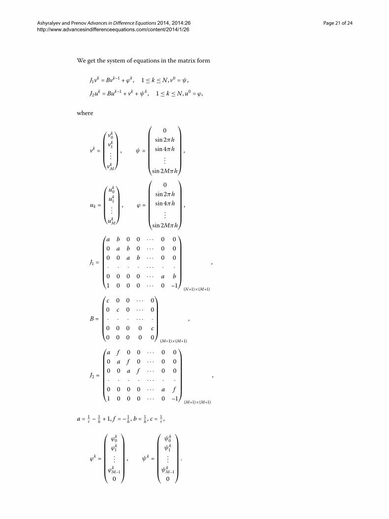
We get the system of equations in the matrix form

Jvk = Bvk– + ϕk , ≤ k ≤N , v =ψ ,

Juk = Buk– + vk +ψk , ≤ k ≤N ,u = ϕ,

where

vk =

⎛⎜⎜⎜⎜⎝vkvk...vkM

⎞⎟⎟⎟⎟⎠ , ψ =

⎛⎜⎜⎜⎜⎜⎜⎜⎝

sinπhsinπh

...sinMπh

⎞⎟⎟⎟⎟⎟⎟⎟⎠,

uk =

⎛⎜⎜⎜⎜⎝ukuk...

ukM

⎞⎟⎟⎟⎟⎠ , ϕ =

⎛⎜⎜⎜⎜⎜⎜⎜⎝

sinπhsinπh

...sinMπh

⎞⎟⎟⎟⎟⎟⎟⎟⎠,

J =

⎛⎜⎜⎜⎜⎜⎜⎜⎜⎝

a b · · · a b · · · a b · · · · · · · · · · · · · · · a b · · · –

⎞⎟⎟⎟⎟⎟⎟⎟⎟⎠

(N+)×(M+)

,

B =

⎛⎜⎜⎜⎜⎜⎜⎝

c · · · c · · · · · · · · · · c

⎞⎟⎟⎟⎟⎟⎟⎠

(M+)×(M+)

,

J =

⎛⎜⎜⎜⎜⎜⎜⎜⎜⎝

a f · · · a f · · · a f · · · · · · · · · · · · · · · a f · · · –

⎞⎟⎟⎟⎟⎟⎟⎟⎟⎠

(M+)×(M+)

,

a = τ–

h + , f = – h , b =

h , c =

τ,

ϕk =

⎛⎜⎜⎜⎜⎜⎜⎜⎝

ϕk

ϕk...

ϕkM–

⎞⎟⎟⎟⎟⎟⎟⎟⎠, ψk =

⎛⎜⎜⎜⎜⎜⎜⎜⎝

ψk

ψk...

ψkM–

⎞⎟⎟⎟⎟⎟⎟⎟⎠.



Table 1 Difference scheme

M = N = 50 M = N = 100

Comparison of errors for u 0.0444 0.0226Comparison of errors for v 0.0875 0.0436

Thus, we have the first-order difference equation with respect to k matrix coefficients. Tosolve this difference equation we have the following procedure:

⎧⎨⎩v

k = J– Bvk– + J– ϕk , ≤ k ≤N , v =ψ ,uk = J– Buk– + J– vk + J– ψk , ≤ k ≤N ,u = ϕ.

()

For their comparison, the errors are computed by

Eu = max≤k≤N–,≤n≤M–

∣∣u(tk ,xn) – ukn∣∣,

Ev = max≤k≤N–,≤n≤M–

∣∣v(tk ,xn) – vkn∣∣

of the numerical solutions. The numerical solutions are recorded for different values ofN = M; ukn, vkn represent the numerical solutions of these difference schemes at (tk ,xn).The errors are given in Table for N =M = , and N =M = , respectively.

6 ConclusionIn the present study, the finite-difference method for the initial-boundary value problemfor the hyperbolic system of equations with nonlocal boundary conditions is studied. Thepositivity of the difference analogy of the space operator generated by this problem inthe space with maximum norm is established. The structure interpolation spaces gener-ated by this difference operator is investigated. The positivity of this difference operator inHölder spaces is established. In practice, stability estimates for the solution of the differ-ence scheme for the hyperbolic system of equations with nonlocal boundary conditionsare obtained. A numerical example is applied. Moreover, applying this approach we canconstruct the stable difference schemes for numerical solutions of the initial-boundaryvalue problem

⎧⎪⎪⎪⎪⎪⎪⎪⎪⎪⎪⎪⎪⎪⎪⎨⎪⎪⎪⎪⎪⎪⎪⎪⎪⎪⎪⎪⎪⎪⎩

∂u(t,x)∂t + a(x) ∂u(t,x)

∂x + δ(u(t,x) – v(t,x)) = f(t,x;u(t,x), v(t,x)), < x < l, < t < T ,

∂v(t,x)∂t – a(x) ∂v(t,x)

∂x + δv(t,x) = f(t,x; v(t,x)), < x < l, < t < T ,

u(t, ) = γu(t, l), ≤ γ ≤ ,βv(t, ) = v(t, l), ≤ β ≤ , ≤ t ≤ T ,u(,x) = u(x), v(,x) = v(x), ≤ x≤ l

()

for the hyperbolic system of semilinear equations with nonlocal boundary conditions. Ofcourse, convergence estimates for the solution of these difference schemes can be ob-tained.



Competing interestsThe authors declare that they have no competing interests.

Authors’ contributionsEach of the authors read and approved the final version of the manuscript.

AcknowledgementsWe would like to thank the reviewers whose careful reading, helpful suggestions, and valuable comments helped us toimprove the manuscript.

Received: 12 October 2013 Accepted: 26 December 2013 Published: 20 Jan 2014

References1. Fattorini, HO: Second Order Linear Differential Equations in Banach Spaces. North-Holland, Amsterdam (1985)2. Goldstein, JA: Semigroups of Linear Operators and Applications. Oxford Mathematical Monographs. Clarendon, New

York (1985)3. Krein, SG: Linear Differential Equations in Banach Space. Nauka, Moscow (1966) (in Russian). English transl.: Linear

Differential Equations in Banach space. Translations of Mathematical Monographs, vol. 23. Am. Math. Soc., Providence(1968)

4. Pogorelenko, V, Sobolevskii, PE: The ‘counter-example’ to W. Littman counter-example of Lp-energetic inequality forwave equation. Funct. Differ. Equ. 4(1-2), 165-172 (1997)

5. Sobolevskii, PE: On the equations of the second order with a small parameter at the highest derivatives. Usp. Mat.Nauk 19(6), 217-219 (1964) (in Russian)

6. Sobolevskii, PE, Semenov, S: On some approach to investigation of singular hyperbolic equations. Dokl. Akad. NaukSSSR 270(1), 555-558 (1983) (in Russian)

7. Vasilev, VV, Krein, SG, Piskarev, S: Operator semigroups, cosine operator functions, and linear differential equations. In:Mathematical Analysis, vol. 28 (in Russian). Itogi Nauki i Tekhniki, vol. 204, pp. 87-202. Akad. Nauk SSSR Vsesoyuz. Inst.Nauchn. i Tekhn. Inform., Moscow (1990). (Translated in J. Soviet Math. 54(4), 1042-1129 (1991))

8. Ashyralyev, A, Fattorini, HO: On uniform difference schemes for second-order singular pertubation problems inBanach spaces. SIAM J. Math. Anal. 23(1), 29-54 (1992)

9. Ashyraliyev, M: A note on the stability of the integral-differential equation of the hyperbolic type in a Hilbert space.Numer. Funct. Anal. Optim. 29(7-8), 750-769 (2008)

10. Yurtsever, A, Prenov, R: On stability estimates for method of line for first order system of differential equations ofhyperbolic type. In: Ashyralyev, A, Yurtsever, A (eds.) Some Problems of Applied Mathematics, pp. 198-205. FatihUniversity Publications, Istanbul (2000)

11. Ashyralyev, A, Yildirim, O: A note on the second order of accuracy stable difference schemes for the nonlocalboundary value hyperbolic problem. Abstr. Appl. Anal. 2012, Article ID 846582 (2012)

12. Ashyralyev, A, Aggez, N: Finite difference method for hyperbolic equations with the nonlocal integral condition.Discrete Dyn. Nat. Soc. 2011, Article ID 562385 (2011)

13. Ashyralyev, A, Sobolevskii, PE: Two new approaches for construction of the high order of accuracy differenceschemes for hyperbolic differential equations. Discrete Dyn. Nat. Soc. 2005(2), 183-213 (2005)

14. Ashyralyev, A, Koksal, ME, Agarwal, RP: A difference scheme for Cauchy problem for the hyperbolic equation withself-adjoint operator. Math. Comput. Model. 52(1-2), 409-424 (2010)

15. Aggez, N, Ashyralyyeva, M: Numerical solution of stochastic hyperbolic equations. Abstr. Appl. Anal. 2012, Article ID824819 (2012)

16. Ashyralyev, A, Akat, M: An approximation of stochastic hyperbolic equations. In: AIP Conference Proceedings,vol. 1389, pp. 625-628 (2011)

17. Amanov, D, Ashyralyev, A: Initial-boundary value problem for fractional partial differential equations of higher order.Abstr. Appl. Anal. 2012, Article ID 973102 (2012)

18. Ashyralyev, A, Dal, F: Finite difference and iteration methods for fractional hyperbolic partial differential equationswith the Neumann condition. Discrete Dyn. Nat. Soc. 2012, Article ID 434976 (2012)

19. Ashyralyev, A, Yildirim, O: On multipoint nonlocal boundary value problems hyperbolic differential and differenceequations. Taiwan. J. Math. 14(1), 165-194 (2010)

20. Soltanov, H: A note on the Goursat problem for a multidimensional hyperbolic equation. Contemp. Anal. Appl. Math.1(2), 98-106 (2013)

21. Selitskii, AM: The space of initial data for the second boundary-value problem for parabolic differential-differenceequation. Contemp. Anal. Appl. Math. 1(1), 34-41 (2013)

22. Selitskii, AM: The space of initial data for the Robin boundary-value problem for parabolic differential-differenceequation. Contemp. Anal. Appl. Math. 1(2), 91-97 (2013)

23. Agarwal, R, Bohner, M, Shakhmurov, VB: Maximal regular boundary value problems in Banach-valued weightedspaces. Bound. Value Probl. 1, 9-42 (2005)

24. Shakhmurov, VB: Coercive boundary value problems for regular degenerate differential-operator equations. J. Math.Anal. Appl. 292(2), 605-620 (2004)

25. Ashyralyev, A, Sobolevskii, PE: Well-posedness of parabolic difference equations. In: Operator Theory Advances andApplications. Birkhäuser, Basel (1994)

26. Rassias, JM, Karimov, ET: Boundary-value problems with non-local condition for degenerate parabolic equations.Contemp. Anal. Appl. Math. 1(1), 42-48 (2013)

27. Ashyralyev, A, Sobolevskii, PE: New difference schemes for partial differential equations. In: Operator TheoryAdvances and Applications. Birkhäuser, Basel (2004)

28. Dehghan, M: On the numerical solution of the diffusion equation with a nonlocal boundary condition. Math. Probl.Eng. 2003(2), 81-92 (2003)

29. Cannon, JR, Perez Esteva, S, van der Hoek, J: A Galerkin procedure for the diffusion equation subject to thespecification of mass. SIAM J. Numer. Anal. 24(3), 499-515 (1987)



30. Gordeziani, N, Natani, P, Ricci, PE: Finite-difference methods for solution of nonlocal boundary value problems.Comput. Math. Appl. 50, 1333-1344 (2005)

31. Dautray, R, Lions, JL: Analyse Mathematique et Calcul Numerique Pour les Sciences et les Techniques, vols. 1-11.Masson, Paris (1988)

32. Ashyralyev, A, Ozdemir, Y: Stability of difference schemes for hyperbolic-parabolic equations. Comput. Math. Appl.50(8-9), 1443-1476 (2005)

33. Ashyralyev, A, Prenov, R: The hyperbolic system of equations with nonlocal boundary conditions. TWMS J. Appl. Eng.Math. 2(2), 154-178 (2012)

34. Godunov, SK: Numerical Methods of Solution of the Equation of Gas Dynamics. NSU, Novosibirsk (1962) (in Russian)35. Tikhonov, AN, Samarskii, AA: Equations of Mathematical Physics. Nauka, Moscow (1977) (in Russian)36. Hersch, R, Kato, T: High accuracy stable difference schemes for well-posed initial value problems. SIAM J. Numer. Anal.

19(3), 599-603 (1982)37. Brenner, P, Crouzeix, M, Thomee, V: Single step methods for inhomogeneous linear differential equations in Banach

space. RAIRO Anal. Numér. 16(1), 5-26 (1982)

10.1186/1687-1847-2014-26Cite this article as: Ashyralyev and Prenov: Finite-difference method for the hyperbolic system of equations withnonlocal boundary conditions. Advances in Difference Equations 2014, 2014:26


finite-difference method for the hyperbolic system of equations with nonlocal boundary conditions

Documents