Finite automata

M. V. Lawson

Department of MathematicsSchool of Mathematical and Computer SciencesHeriot-Watt UniversityRiccarton, Edinburgh EH14 4ASScotlandM.V.Lawson@ma.hw.ac.uk

1 Introduction

The term ‘finite automata’ describes a class of models of computation thatare characterised by having a finite number of states. The use of the word ‘au-tomata’ harks back to the early days of the subject in the 1950’s when theywere viewed as abstract models of real circuits. However, the readers of thischapter can also view them as being implemented by programming languages,or as themselves constituting a special class of programming languages. Takingthis latter viewpoint, finite automata form a class of programming languageswith very restricted operation sets: roughly speaking, programs where thereis no recursion or looping. In particular, none of them is a universal program-ming language; indeed, it is possible to prove that some quite straightforwardoperations cannot be programmed even with the most general automata Idiscuss. Why, then, should anyone be interested in programming with, as itwere, one hand tied behind their back? The answer is that automata turn outto be useful — so they are not merely mathematical curiosities. In addition,because they are restricted in what they can do, we can actually say moreabout them, which in turn helps us manipulate them.

The most general model I discuss in this chapter is that of a finite trans-ducer, in Section 3.3, but I build up to this model in Sections 2, 3.1, and 3.2by discussing, in increasing generality: finite acceptors, finite purely sequen-tial transducers, and finite sequential transducers. The finite acceptors formthe foundation of the whole enterprise through their intimate link with regu-lar expressions and, in addition, they form the pattern after which the moregeneral theories are modelled.

What then are the advantages of the various kinds of finite transducersconsidered in this chapter? There are two main ones: the speed with whichdata can be processed by such a device, and the algorithms that enable oneto make the devices more efficient. The fact that finite transducers of vari-

2 M. V. Lawson

ous kinds have turned out to be useful in natural language processing is atestament to both of these advantages [23]. I discuss the advantages of finitetransducers in a little more detail in Section 4.

To read this chapter, I have assumed that you have been exposed to a firstcourse in discrete math(s); you need to know a little about sets, functions, andrelations, but not much more. My goal has been to describe the core of thetheory in the belief that once the basic ideas have been grasped, the businessof adding various bells and whistles can easily be carried out according totaste.

Other reading There are two classic books outlining the theory of finitetransducers: Berstel [4] and Eilenberg [12]. Of these, I find Berstel’s 1979book the more accessible. However, the theory has moved on since 1979, andin the course of this chapter I refer to recent papers that take the subject upto the present day. In particular, the paper [24] contains a modern, mathemat-ical approach to the basic theory of finite transducers. The book by JacquesSakarovitch [30] is a recent account of automata theory that is likely to becomea standard reference. The chapters by Berstel and Perrin [6], on algorithms onwords, and by Laporte [21], on symbolic natural language processing, both tobe found in the forthcoming book by M. Lothaire, are excellent introductionsto finite automata and their applications. The articles [25] and [35] are inter-esting in themselves and useful for their lengthy bibliographies. My chapterdeals entirely with finite strings — for the theory of infinite strings see [26].Finally, finite transducers are merely a part of theoretical computer science;for the big picture, see [17].

Terminology This has not been entirely standardised so readers should be ontheir guard when reading papers and books on finite automata. Throughoutthis chapter I have adopted the following terminology introduced by JacquesSakarovitch and suggested to me by Jean-Eric Pin: a ‘purely sequential func-tion’ is what is frequently referred to in the literature as a ‘sequential function’;whereas a ‘sequential function’ is what is frequently referred to as a ‘subse-quential function’. The new terminology is more logical than the old, andsignals more clearly the role of sequential functions (in the new sense).

2 Finite Acceptors

The automata in this section might initially not seem very useful: their re-sponse to an input is to output either a ‘yes’ or a ‘no’. However, the conceptsand ideas introduced here provide the foundation for the rest of the chapter,and a model for the sorts of things that finite automata can do.

Finite automata 3

2.1 Alphabets, strings, and languages

Information is encoded by means of sequences of symbols. Any finite setA usedto encode information will be called an alphabet, and any finite sequence whosecomponents are drawn from A is called a string over A or simply a string,and sometimes a word. We call the elements of an alphabet symbols, letters,or tokens. The symbols in an alphabet do not have to be especially simple;an alphabet could consist of pictures, or each element of an alphabet coulditself be a sequence of symbols. A string is formally written using brackets andcommas to separate components. Thus (now, is, the,winter, of, our,discontent)is a string over the alphabet whose symbols are the words in an Englishdictionary. The string () is the empty string. However, we shall write stringswithout brackets and commas and so, for instance, we write 01110 ratherthan (0, 1, 1, 1, 0). The empty string needs to be recorded in some way and wedenote it by ε. The set of all strings over the alphabet A is denoted by A∗,read ‘A star’. If w is a string then |w | denotes the total number of symbolsappearing in w and is called the length of w. Observe that | ε | = 0. It is worthnoting that two strings u and v over an alphabet A are equal if they containthe same symbols in the same order.

Given two strings x, y ∈ A∗, we can form a new string x · y, called theconcatenation of x and y, by simply adjoining the symbols in y to those inx. We shall usually denote the concatenation of x and y by xy rather thanx · y. The string ε has a special property with respect to concatenation: foreach string x ∈ A∗ we clearly have that εx = x = xε. It is important toemphasise that the order in which strings are concatenated is important: thusxy is generally different from yx.

There are many definitions concerned with strings, but for this chapter Ijust need two. Let x, y ∈ A∗. If u = xy then x is called a prefix of u, and y iscalled a suffix of u.

Alphabets and strings are needed to define the key concept of this section:that of a language. Before formally defining this term, here is a motivatingexample.

Example 1. Let A be the alphabet that consists of all words in an Englishdictionary; so we regard each English word as being a single symbol. The setA∗ consists of all possible finite sequences of words. Define the subset L of A∗

to consist of all sequences of words that form grammatically correct Englishsentences. Thus

to be or not to be∈ L

whereas

be be to to or not /∈ L.

Someone who wants to understand English has to learn the rules for decidingwhen a string of words belongs to the set L. We can therefore think of L asbeing the English language.

4 M. V. Lawson

For any alphabet A, any subset of A∗ is called an A-language or a languageover A or simply a language. Languages are usually infinite; the question weshall address in Section 2.2 is to find a finite way of describing (some) infinitelanguages.

There are a number of ways of combining languages to make new ones. IfL and M are languages over A so are L ∩M , L ∪M , and L′: respectively,the intersection of L and M , the union of L and M , and the complement ofL. These are called the Boolean operations and come from set theory. Recallthat ‘x ∈ L ∪M ’ means ‘x ∈ L or x ∈ M or both.’ In automata theory, weusually write L+M rather than L ∪M when dealing with languages. Thereare two further operations on languages that are peculiar to automata theoryand extremely important: the product and the Kleene star. Let L and M belanguages. Then

L ·M = {xy: x ∈ L and y ∈M}

is called the product of L and M . We usually write LM rather than L ·M . Astring belongs to LM if it can be written as a string in L followed by a stringinM . For a language L, we define L0 = {ε}, and Ln+1 = Ln ·L. For n > 0, thelanguage Ln consists of all strings u of the form u = x1 . . . xn where xi ∈ L.The Kleene star of a language L, denoted L∗, is defined to be

L∗ = L0 + L1 + L2 + . . . .

2.2 Finite acceptors

An information-processing device transforms inputs into outputs. In general,there are two alphabets associated with such a device: an input alphabet A forcommunicating with it, and an output alphabet B for receiving answers. Forexample, consider a device that takes as input sentences in English and out-puts the corresponding sentence in Russian. In later sections, I shall describemathematical models of such devices of increasing generality. In this section,I shall look at a special case: there is an input alphabet A, but each inputstring causes the device to output either ‘yes’ or ‘no’ once the whole inputhas been processed. Those input strings from A∗ that cause the machine tooutput ‘yes’ are said to be accepted by the machine, and those that cause itto output ‘no’ are said to be rejected. In this way, A∗ is partitioned into twosubsets: the ‘yes’ subset we call the language accepted by the machine, andthe ‘no’ subset we call the language rejected by the machine. A device thatoperates in this way is called an acceptor. We shall describe a mathematicalmodel of a special class of acceptors. Our goal is to describe potentially infinitelanguages by finite means.

A finite (deterministic) acceptorA is specified by five pieces of information:

A = (S,A, i, δ, T ) ,

where S is a finite set called the set of states, A is the finite input alphabet, iis a fixed element of S called the initial state, δ is a function δ: S × A → S,

Finite automata 5

called the transition function, and T is a subset of S (possibly empty!) calledthe set of terminal or final states.

There are two ways of providing the five pieces of information needed tospecify an acceptor: transition diagrams and transition tables. A transitiondiagram is a special kind of directed labelled graph: the vertices are labelledby the states S of A; there is an arrow labelled a from the vertex labelleds to the vertex labelled t precisely when δ(s, a) = t in A. That is to say,the input a causes the acceptor A to change from state s to state t. Finally,the initial state and terminal states are distinguished in some way: we mark

the initial state by an inward-pointing arrow, // i?>=<89:;, and the terminal

states by double circles t?>=<89:;'&%$Ã!"# . A transition table is just a way of describing the

transition function δ in tabular form and making clear in some way the initialand terminal states. The table has rows labelled by the states and columnslabelled by the input letters. At the intersection of row s and column a weput the element δ(s, a). The states labelling the rows are marked to indicatethe initial state and the terminal states.

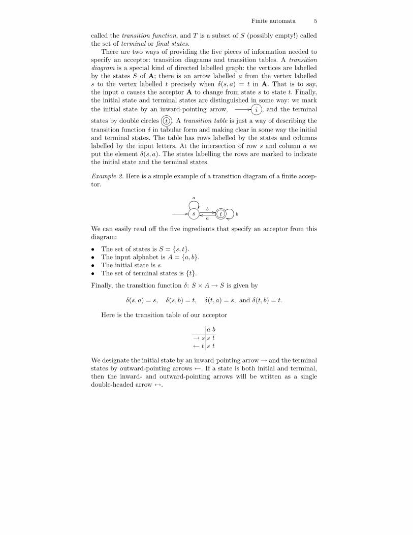
Example 2. Here is a simple example of a transition diagram of a finite accep-tor.

//?>=<89:;sa

¨¨ b //?>=<89:;/.-,()*+t bggaoo

We can easily read off the five ingredients that specify an acceptor from thisdiagram:

• The set of states is S = {s, t}.• The input alphabet is A = {a, b}.• The initial state is s.• The set of terminal states is {t}.

Finally, the transition function δ: S ×A→ S is given by

δ(s, a) = s, δ(s, b) = t, δ(t, a) = s, and δ(t, b) = t.

Here is the transition table of our acceptor

a b→ s s t← t s t

We designate the initial state by an inward-pointing arrow→ and the terminalstates by outward-pointing arrows ←. If a state is both initial and terminal,then the inward- and outward-pointing arrows will be written as a singledouble-headed arrow ↔.

6 M. V. Lawson

To avoid too many arrows cluttering up a transition diagram, the followingconvention is used: if the letters a1, . . . , am label m transitions from the states to the state t, then we simply draw one arrow from s to t labelled a1, . . . , am

rather than m arrows labelled a1 to am, respectively.Let A be a finite acceptor with input alphabet A and initial state i. For

each state q of A and for each input string x, there is a unique path in A

that begins at q and is labelled by the symbols in x in turn. This path endsat a state we denote by q · x. We say that x is accepted by A if i · x is aterminal state. That is, x labels a path in A that begins at the initial stateand ends at a terminal state. Define the language accepted or recognised byA, denoted L(A), to be the set of all strings in the input alphabet that areaccepted by A. A language is said to be recognisable if it is accepted by somefinite automaton. Observe that the empty string is accepted by an automatonif and only if the initial state is also terminal.

Example 3.We describe the language recognised by our acceptor in Exam-ple 2. We have to find all those strings in (a+ b)∗ that label paths starting ats and finishing at t. First, any string x ending in a ‘b’ will be accepted. To seewhy, let x = x′b where x′ ∈ A∗. If x′ leads the acceptor to state s, then the bwill lead the acceptor to state t; and if x′ leads the acceptor to state t, thenthe b will keep it there. Second, a string x ending in ‘a’ will not be accepted.To see why, let x = x′a where x′ ∈ A∗. If x′ leads the acceptor to state s, thenthe a will keep it there; and if x′ leads the acceptor to state t, then the a willsend it to state s. We conclude that L(A) = A∗{b}.

Here are some further examples of recognisable languages. I leave it as anexercise to the reader to construct suitable finite acceptors.

Example 4. Let A = {a, b}.

(i) The empty set ∅ is recognisable.(ii) The language {ε} is recognisable.(iii) The languages {a} and {b} are recognisable.

It is worth pointing out that not all languages are recognisable. For ex-ample, the language consisting of those strings of a’s and b’s having an equalnumber of a’s and b’s is not recognisable.

One very important feature of finite (deterministic) acceptors needs tobe highlighted, since it has great practical importance. The time taken for afinite acceptor to determine whether a string is accepted or rejected is a linearfunction of the length of the string; once a string has been completely read,we will have our answer.

The classic account of the theory of finite acceptors and their languagesis contained in the first three chapters of [16]. The first two chapters of mybook [22] describe the basics of finite acceptors at a more elementary level.

Finite automata 7

2.3 Non-deterministic ε-acceptors

The task of constructing a finite acceptor to recognise a given language canbe a frustrating one. The chief reason for the difficulty is that finite acceptorsare quite rigid: they have one initial state, and for each input letter and eachstate exactly one transition. Our first step, then, will be to relax these twoconditions.

A finite non-deterministic acceptor A is determined by five pieces of in-formation:

A = (S,A, I, δ, T ),

where S is a finite set of states, A is the input alphabet, I is a set of initialstates, δ: S × A → P(S) is the transition function, where P(S) is the set ofall subsets of S, and T is a set of terminal states. In addition to allowingany number of initial states, the key feature of this definition is that δ(s, a)is now a subset of S, possibly empty. The transition diagrams and transitiontables we defined for deterministic acceptors can easily be adapted to describenon-deterministic ones. If q is a state and x a string, then the set of all statesq′ for which there is a path in A beginning at q, ending at q′, and labelled byx is denoted by q · x. The language L(A) recognised by a non-deterministicacceptor consists of all those strings in A∗ that label a path in A from at leastone of the initial states to at least one of the terminal states.

It might be thought that, because there is a degree of choice available,non-deterministic acceptors might be able to recognise languages that deter-ministic ones could not. In fact, this is not so.

Theorem 1. Let A be a finite non-deterministic acceptor. Then there is analgorithm for constructing a deterministic acceptor, Ad, such that L(Ad) =L(A).

We now introduce a further measure of flexibility in constructing acceptors.In both deterministic and non-deterministic acceptors, transitions may onlybe labelled with elements of the input alphabet; no edge may be labelledwith the empty string ε. We shall now waive this restriction. A finite non-deterministic acceptor with ε-transitions or, more simply, a finite ε-acceptor,is a 5-tuple,

A = (S,A, I, δ, T ),

where all the symbols have the same meanings as in the non-deterministiccase except that now

δ: S × (A ∪ {ε})→ P(S).

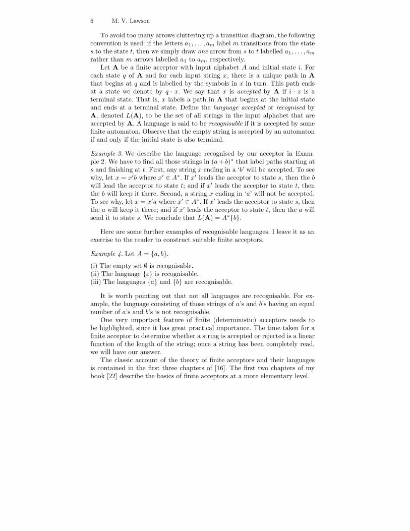
The only difference between such acceptors and non-deterministic ones is thatwe allow transitions, called ε-transitions, of the form

//?>=<89:;s ε //?>=<89:;t

8 M. V. Lawson

A path in an ε-acceptor is a sequence of states each labelled by an elementof the set A∪ {ε}. The string corresponding to this path is the concatenationof these labels in order; it is important to remember at this point that forevery string x we have that εx = x = xε. We say that a string x is acceptedby an ε-automaton if there is a path from an initial state to a terminal statethe concatenation of whose labels is x.

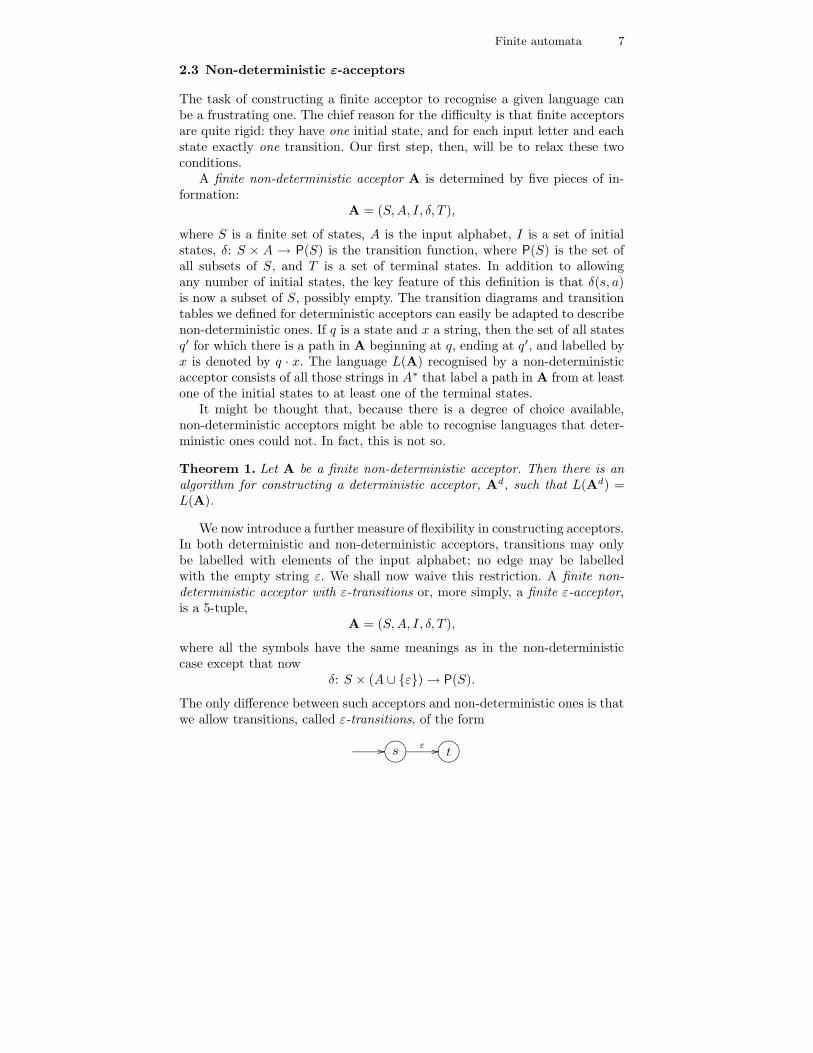
Example 5. Consider the following finite ε-acceptor:

///.-,()*+ ε //

a

²²

/.-,()*+b

²²/.-,()*+ε

ÂÂ???

????

? /.-,()*+ε

²²/.-,()*+ÂÁÀ¿»¼½¾The language it recognises is {a, b}. The letter a is recognised because

aε labels a path from the initial to the terminal state, and the letter b isrecognised because εbε labels a path from the initial to the terminal state.

The existence of ε-transitions introduces a further measure of flexibilityin building acceptors but, as the following theorem shows, we can convertsuch acceptors to non-deterministic automata without changing the languagerecognised.

Theorem 2. Let A be a finite ε-acceptor. Then there is an algorithm thatconstructs a non-deterministic acceptor without ε-transitions, As, such thatL(As) = L(A).

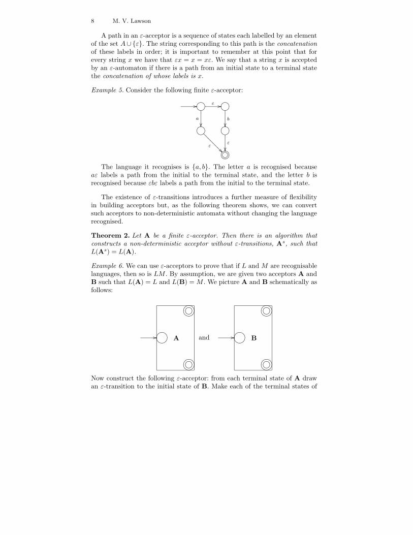
Example 6.We can use ε-acceptors to prove that if L and M are recognisablelanguages, then so is LM . By assumption, we are given two acceptors A andB such that L(A) = L and L(B) =M . We picture A and B schematically asfollows:

?>=<89:;'&%$Ã!"#

//?>=<89:; A

?>=<89:;'&%$Ã!"#

and

?>=<89:;'&%$Ã!"#

//?>=<89:; B

?>=<89:;'&%$Ã!"#Now construct the following ε-acceptor: from each terminal state of A drawan ε-transition to the initial state of B. Make each of the terminal states of

Finite automata 9

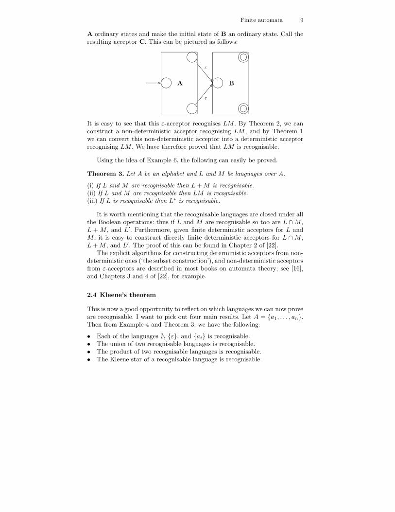
A ordinary states and make the initial state of B an ordinary state. Call theresulting acceptor C. This can be pictured as follows:

?>=<89:;ε

¿¿999

9999

9?>=<89:;'&%$Ã!"#

//?>=<89:; A ?>=<89:; B

?>=<89:;ε

BB¦¦¦¦¦¦¦¦ ?>=<89:;'&%$Ã!"#It is easy to see that this ε-acceptor recognises LM . By Theorem 2, we canconstruct a non-deterministic acceptor recognising LM , and by Theorem 1we can convert this non-deterministic acceptor into a deterministic acceptorrecognising LM . We have therefore proved that LM is recognisable.

Using the idea of Example 6, the following can easily be proved.

Theorem 3. Let A be an alphabet and L and M be languages over A.

(i) If L and M are recognisable then L+M is recognisable.(ii) If L and M are recognisable then LM is recognisable.(iii) If L is recognisable then L∗ is recognisable.

It is worth mentioning that the recognisable languages are closed under allthe Boolean operations: thus if L and M are recognisable so too are L ∩M ,L +M , and L′. Furthermore, given finite deterministic acceptors for L andM , it is easy to construct directly finite deterministic acceptors for L ∩M ,L+M , and L′. The proof of this can be found in Chapter 2 of [22].

The explicit algorithms for constructing deterministic acceptors from non-deterministic ones (‘the subset construction’), and non-deterministic acceptorsfrom ε-acceptors are described in most books on automata theory; see [16],and Chapters 3 and 4 of [22], for example.

2.4 Kleene’s theorem

This is now a good opportunity to reflect on which languages we can now proveare recognisable. I want to pick out four main results. Let A = {a1, . . . , an}.Then from Example 4 and Theorem 3, we have the following:

• Each of the languages ∅, {ε}, and {ai} is recognisable.• The union of two recognisable languages is recognisable.• The product of two recognisable languages is recognisable.• The Kleene star of a recognisable language is recognisable.

10 M. V. Lawson

Call a language over an alphabet basic if it is either empty, consists of theempty string alone, or consists of a single symbol from the alphabet. Thenwhat we have proved is the following: a language that can be constructed fromthe basic languages by using only the operations +, ·, and ∗ a finite number oftimes must be recognisable. Such a language is said to be regular or rational.

Example 7. Consider the language L over the alphabet {a, b} that consists ofall strings of even length. We shall show that this is a regular language. Astring of even length is either empty, or can be written as a product of stringsof length 2. Conversely every string that can be written as a product of stringsof length 2 has even length. It follows that

L = ((({a}{a}+ {a}{b}) + {b}{a}) + {b}{b})∗.

Thus L is regular.

In the example above, we would much rather write

L = (aa+ ab+ ba+ bb)∗

for clarity. How to do this in general is formalised in the notion of a ‘regularexpression.’ Let A = {a1, . . . , an} be an alphabet. A regular expression (overA) or rational expression (over A) is a sequence of symbols formed by repeatedapplication of the following rules:

(R1) ∅ is a regular expression.(R2) ε is a regular expression.(R3) a1, . . . , an are each regular expressions.(R4) If s and t are regular expressions then so is (s+ t).(R5) If s and t are regular expressions then so is (s · t).(R6) If s is a regular expression then so is (s∗).(R7) Every regular expression arises by a finite number of applications of the

rules (R1) through (R6).

As usual, we will write st rather than s · t. Each regular expression s describesa regular language, denoted by L(s). This language is calculated by means ofthe following rules. Simply put, they tell us how to ‘insert the curly brackets.’

(D1) L(∅) = ∅.(D2) L(ε) = {ε}.(D3) L(ai) = {ai}.(D4) L(s+ t) = L(s) + L(t).(D5) L(s · t) = L(s) · L(t).(D6) L(s∗) = L(s)∗.

It is also possible to get rid of many of the left and right brackets that occur in aregular expression by making conventions about the precedence of the regularoperators. When this is done, regular expressions form a useful notation for

Finite automata 11

describing regular languages. However, if a language is described in some otherway, it may be necessary to carry out some work to find a regular expressionthat describes it; Example 7 illustrates this point.

The first major result in automata theory is the following, known asKleene’s theorem.

Theorem 4. A language is recognisable if and only if it is regular. In par-ticular, there are algorithms that accept as input a regular expression r, andoutput a finite acceptor A such that L(A) = L(r); and there are algorithmsthat accept as input a finite acceptor A, and output a regular expression rsuch that L(r) = L(A).

This theorem is significant for two reasons: first, it tells us that there isan algorithm that enables us to construct an acceptor recognising a languagefrom a suitable description of that language; second, it tells us that there isan algorithm that will produce a description of the language recognised by anacceptor.

A number of different proofs of Kleene’s theorem may be found in Chap-ter 5 of [22]. For further references on how to convert regular expressions intofinite acceptors, see [5] and [7]. Regular expressions as I have defined them areuseful for proving Kleene’s theorem but hardly provide a convenient tool fordescribing regular languages over realistic alphabets containing large numbersof symbols. The practical side of regular expressions is described by Friedl [14]who shows how to use regular expressions to search texts.

2.5 Minimal automata

In this section, I shall describe an important feature of finite acceptors thatmakes them particularly useful in applications: the fact that they can beminimised. I have chosen to take the simplest approach in describing thisproperty, but at the end of this section, I describe a more sophisticated oneneeded in generalisations.

Given a recognisable language L, there will be many finite acceptors thatrecognise L. All things being equal, we would usually want to pick the smallestsuch acceptor: namely, one having the smallest number of states. It is conceiv-able that there could be two different acceptors A1 and A2 both recognisingL, both having the same number of states, and sharing the additional propertythat there is no acceptor with fewer states recognising L. In this section, I shallexplain why this cannot happen. This result has an important consequence:every recognisable language is accepted by an essentially unique smallest ac-ceptor. To show that this is true, we begin by showing how an acceptor maybe reduced in size without changing the language recognised. There are twomethods that can be applied, each dealing with a different kind of inefficiency.

The first method removes states that cannot play any role in decidingwhether a string is accepted. Let A = (S,A, i, δ, T ) be a finite acceptor. We

12 M. V. Lawson

say that a state s ∈ S is accessible if there is a string x ∈ A∗ such that i·x = s.Observe that the initial state itself is always accessible because i · ε = i. Astate that is not accessible is said to be inaccessible. An acceptor is said to beaccessible if every state is accessible. It is clear that the inaccessible states ofan automaton can play no role in accepting strings; consequently, we expectthat they could be removed without the language being changed. This turnsout to be the case.

Theorem 5. Let A be a finite acceptor. Then there is an algorithm that con-structs an accessible acceptor, Aa, such that L(Aa) = L(A).

The second method identifies states that ‘do the same job.’ Let A =(S,A, i, δ, T ) be an acceptor. Two states s, t ∈ S are said to be distinguishableif there exists x ∈ A∗ such that

(s · x, t · x) ∈ (T × T ′) ∪ (T ′ × T ),

where T ′ is the set of non-terminal states. In other words, for some string x,one of the states s · x and t · x is terminal and the other non-terminal. Thestates s and t are said to be indistinguishable if they are not distinguishable.This means that for each x ∈ A∗ we have that

s · x ∈ T ⇔ t · x ∈ T.

Define the relation 'A on the set of states S by

s 'A t⇔ s and t are indistinguishable.

We call'A the indistinguishability relation, and it is an equivalence relation. Itcan happen, of course, that each pair of states in an acceptor is distinguishable:in other words, the relation 'A is equality. We say that such an acceptor isreduced.

Theorem 6. Let A be a finite acceptor. Then there is an algorithm that con-structs a reduced acceptor, Ar, such that L(Ar) = L(A).

Our two methods can be applied to an acceptor A in turn yielding anacceptor Aar = (Aa)r that is both accessible and reduced. The reader maywonder at this point whether there are other methods for removing states.We shall see that there are not.

We now come to a fundamental definition. Let L be a recognisable lan-guage. A finite deterministic acceptor A is said to be minimal (for L) ifL(A) = L, and if B is any finite acceptor such that L(B) = L, then the num-ber of states of A is less than or equal to the number of states of B. Minimalacceptors for a language L certainly exist. The problem is to find a way ofconstructing them. Our search is narrowed down by the following observationwhose simple proof is left as an exercise: if A is minimal for L, then A is bothaccessible and reduced.

Finite automata 13

In order to realise the main goal of this section, we need to have a precisemathematical definition of when two acceptors are essentially the same: onethat we can check in a systematic way however large the automata involved.The definition below provides the answer to this question.

Let A = (S,A, s0, δ, F ) and B = (Q,A, q0, γ,G) be two acceptors withthe same input alphabet A. An isomorphism θ from A to B is a functionθ: S → Q satisfying the following four conditions:

(IM1) The function θ is bijective.(IM2) θ(s0) = q0.(IM3) s ∈ F ⇔ θ(s) ∈ G.(IM4) θ(δ(s, a)) = γ(θ(s), a) for each s ∈ S and a ∈ A.

If there is an isomorphism from A to B we say that A is isomorphicto B. Isomorphic acceptors may differ in their state labelling and may lookdifferent when drawn as directed graphs, but by suitable relabelling, and bymoving states and bending transitions, they can be made to look identical.Thus isomorphic automata are ‘essentially the same’ meaning that they differin only trivial ways.

Theorem 7. Let L be a recognisable language. Then L has a minimal accep-tor, and any two minimal acceptors for L are isomorphic. A reduced accessibleacceptor recognising L is a minimal acceptor for L.

Remark It is worth reflecting on the significance of this theorem, particularlysince in the generalisations considered later in this chapter, a rather moresubtle notion of ‘minimal automaton’ has to be used. Theorem 7 tells us thatif by some means we can find an acceptor for a language, then by applyinga couple of algorithms, we can convert it into the smallest possible acceptorfor that language. This should be contrasted with the situation for arbitraryproblems where, if we find a solution, there are no general methods for makingit more efficient, and where the concept of a smallest solution does not evenmake sense. The above theorem is therefore one of the benefits of workingwith a restricted class of operations.

The approach I have adopted to describing a minimal acceptor can begeneralised in a straightforward fashion to the Moore and Mealy machines Idescribe in Section 3.1. However, when I come to the sequential transducers ofSection 3.2, this naive approach breaks down. In this case, it is indeed possibleto have two sequential transducers that do the same job, are as small as possi-ble, but which are not isomorphic. A specific example of this phenomenon canbe found in [27]. However, it transpires that we can still pick out a ‘canonicalmachine’ that also has the smallest possible number of states. The construc-tion of this canonical machine needs slightly more sophisticated mathematics;I shall outline how this approach can be carried out for finite acceptors.

The finite acceptors I have defined are technically speaking the ‘completefinite acceptors.’ An incomplete finite acceptor is defined in the same way asa complete one except that we allow the transition function to be a partial

14 M. V. Lawson

function. Clearly, we can convert an incomplete acceptor into a complete oneby adjoining an extra state and defining appropriate transitions. However,there is no need to do this: incomplete acceptors bear the same relationshipto complete ones as partial functions do to (globally defined) functions, and incomputer science it is the partial functions that are the natural functions toconsider. For the rest of this paragraph, ‘acceptor’ will mean one that could beincomplete. One way of simplifying an acceptor is to remove the inaccessiblestates. Another way of simplifying an acceptor is to remove those states s forwhich there is no string x such that s · x is terminal. An acceptor with theproperty that for each state s there is a string x such that s · x is terminal issaid to be coaccessible. Clearly, if we prune an acceptor of those states thatare not coaccessible, the resulting acceptor is coaccessible. The reader shouldobserve that if this procedure is carried out on a complete acceptor, then theresulting acceptor could well be incomplete. This is why I did not define thisnotion earlier. Acceptors that are both accessible and coaccessible are saidto be trim. It is possible to define what we mean by a ‘morphism’ betweenacceptors; I shall not make a formal definition here, but I will explain howthey can be used. Let L be a recognisable language, and consider all the trimacceptors recognising L. If A and B are two such acceptors, it can be provedthat there is at most one morphism from A to B. If there is a morphism fromA to B, and from B to A, then A and B are said to be ‘isomorphic’; thishas the same significance as my earlier definition of isomorphic. The key pointnow is this:

there is a distinguished trim acceptor AL recognising L characterisedby the property that for each trim acceptor A recognising L there is a,necessarily unique, morphism from A to AL.

It turns out that AL can be obtained from A by a slight generalisation of thereduction process I described earlier. By definition, AL is called the minimalacceptor for L. It is a consequence of the defining property of AL that AL hasthe smallest number of states amongst all the trim acceptors recognising L.The reader may feel that this description of the minimal acceptor merely com-plicates my earlier, more straightforward, description. However, the importantpoint is this: the characterisation of the minimal acceptor in the terms I havehighlighted above generalises, whereas its characterisation in terms of havingthe smallest possible number of states does not. A full mathematical justifi-cation of the claims made in this paragraph can be found in Chapter III of [12].

A simple algorithm for minimising an acceptor and an algorithm for con-structing a minimal acceptor from a regular expression are described in Chap-ter 7 of [22]. For an introduction to implementing finite acceptors and theirassociated algorithms, see [34].

Finite automata 15

3 Finite Transducers

In Section 2, I outlined the theory of finite acceptors. This theory tells usabout devices where the response to an input is simply a ‘yes’ or a ‘no’. Inthis section, I describe devices that generalise acceptors but generate outputsthat provide more illuminating answers to questions. Section 3.1 describeshow to modify acceptors so that they generate output. It turns out that thereare two ways to do this: either to associate outputs with states, or to associateoutputs with transitions. The latter approach is the one adopted for general-isations. Section 3.2 describes the most general way of generating output in asequential fashion, and Section 3.3 describes the most general model of ‘finitestate devices.’

3.1 Finite purely sequential transducers

I shall begin this section by explaining how finite acceptors can be adaptedto generate outputs.

A language L is defined to be a subset of some A∗, where A is any alphabet.Subsets of sets can also be defined in terms of functions. To see how, let Xbe a set, and let Y ⊆ X be any subset. Define a function

χY : X → 2 = {0, 1}

by

χY (x) =

{

1 if x ∈ Y0 if x /∈ Y .

The function χY , which contains all the information about which elementsbelong to the subset Y , is called the characteristic function of the subset Y .More generally, any function

χ: X → 2

defines a subset of X: namely, the set of all x ∈ X such that χ(x) = 1. Itis not hard to see that subsets of X and characteristic functions on X areequivalent ways of describing the same thing. It follows that languages overA can be described by functions χ: A∗ → 2, and vice versa.

Suppose now that L is a language recognised by the acceptor A =(Q,A, i, δ, T ). We should like to regard A as calculating the characteristicfunction χL of L. To do this, we need to make some minor alterations to A.Rather than labelling a state as terminal, we shall instead add the label ‘1’ tothe state; thus if the state q is terminal, we shall relabel it as q/1. If a state qis not terminal, we shall relabel it as q/0. Clearly with this labelling, we candispense with the set T since it can be recovered as those states q labelled ‘1’.What we have done is define a function λ: Q → 2. Our ‘automaton’ is nowdescribed by the following information: B = (Q,A,2, q0, δ, λ). To see how thisautomaton computes the characteristic function, we need an auxilliary func-tion ωB: A

∗ → (0 + 1)∗, which is defined as follows. Let x = x1 . . . xn be a

16 M. V. Lawson

string of length n over A, and let the states B passes through when processingx be q0, q1, . . . , qn. Thus

q0x1−→ q1

x2−→ . . .xn−→ qn.

Define the stringωB(x) = λ(q0)λ(q1) . . . λ(qn).

Thus ωB: A∗ → (0 + 1)∗ is a function such that

ωB(ε) = λ(q0) and |ωB(x)| = |x|+ 1.

The characteristic function of the language L(A) is the function ρωB: A∗ → 2,

where ρ is the function that outputs the rightmost letter of a non-empty string.For the automaton B, I have defined two functions: ωB: A

∗ → (0 + 1)∗,which I shall call the output response function of the automaton B, andχB: A

∗ → 2, which I shall call the characteristic function of the automa-ton B. I shall usually just write ω and χ when the automaton in question isclear. We have noted already that χ = ρω. On the other hand,

ω(x1 . . . xn) = χ(ε)χ(x1)χ(x1x2) . . . χ(x1 . . . xn).

Thus knowledge of either one of ω and χ is enough to determine the other;both are legitimate output functions, and which one we use will be decidedby the applications we have in mind. To make these ideas more concrete, hereis an example.

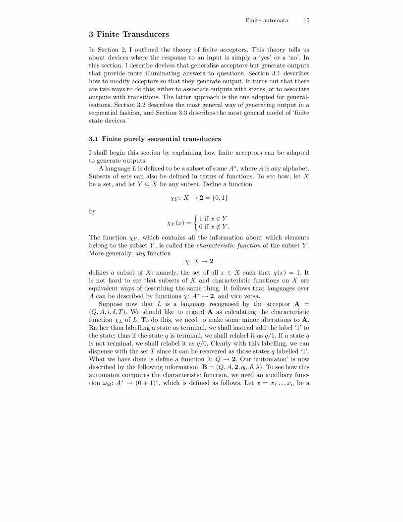
Example 8. Consider the finite acceptor A below

// GFED@ABC?>=<89:;q a,b // GFED@ABCra,b

oo

The language L(A) consists of all those strings in (a+ b)∗ of even length.We now convert it into the automaton B described above

// ONMLHIJKq/1a,b // ONMLHIJKr/0a,b

oo

We can calculate the value of the output response function ω: (a + b)∗ →(0 + 1)∗ on the string aba by observing that in processing this string we passthrough the four states: q, r, q, and r. Thus ω(aba) = 1010. By definition,χ(aba) = 0.

There is nothing sacrosanct about the set 2 having two elements. Wecould just as well replace it by any alphabet B, and so view an automaton ascomputing functions from A∗ to B. This way of generating output from anautomaton leads to the following definition.

Finite automata 17

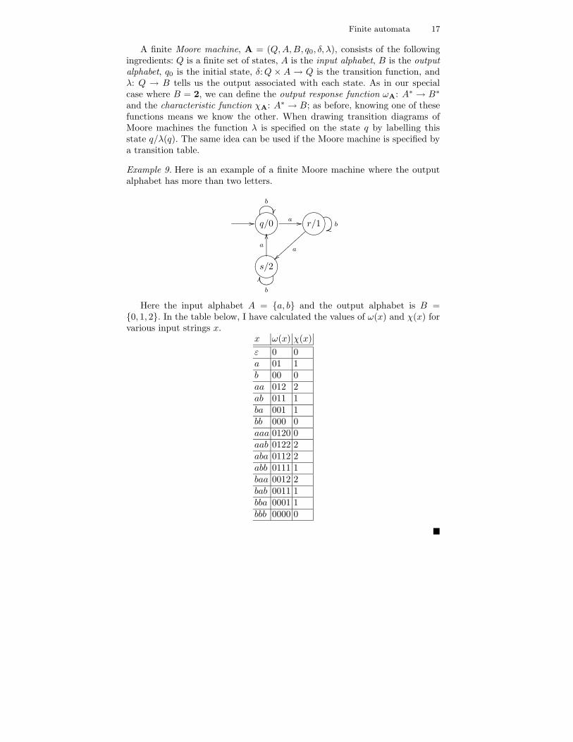
A finite Moore machine, A = (Q,A,B, q0, δ, λ), consists of the followingingredients: Q is a finite set of states, A is the input alphabet, B is the outputalphabet, q0 is the initial state, δ:Q × A → Q is the transition function, andλ: Q → B tells us the output associated with each state. As in our specialcase where B = 2, we can define the output response function ωA: A∗ → B∗

and the characteristic function χA: A∗ → B; as before, knowing one of thesefunctions means we know the other. When drawing transition diagrams ofMoore machines the function λ is specified on the state q by labelling thisstate q/λ(q). The same idea can be used if the Moore machine is specified bya transition table.

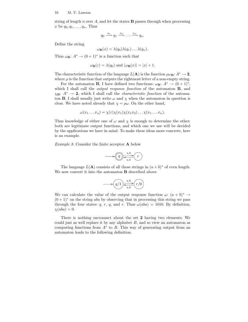
Example 9. Here is an example of a finite Moore machine where the outputalphabet has more than two letters.

// ONMLHIJKq/0

b

¯¯a // ONMLHIJKr/1 bqq

a

}}|||||||||

ONMLHIJKs/2

a

OO

b

LL

Here the input alphabet A = {a, b} and the output alphabet is B ={0, 1, 2}. In the table below, I have calculated the values of ω(x) and χ(x) forvarious input strings x.

x ω(x) χ(x)

ε 0 0a 01 1b 00 0aa 012 2ab 011 1ba 001 1bb 000 0aaa 0120 0aab 0122 2aba 0112 2abb 0111 1baa 0012 2bab 0011 1bba 0001 1bbb 0000 0

¥

18 M. V. Lawson

It is natural to ask under what circumstances a function f : A∗ → Bis the characteristic function of some finite Moore machine. One answer tothis question is provided by the theorem below, which can be viewed as anapplication of Kleene’s theorem. For a proof see Theorem XI.6.1 of [12].

Theorem 8. Let f : A∗ → B be an arbitrary function. Then there is a finiteMoore machine A with input alphabet A and output alphabet B such thatf = χA, the characteristic function of A, if and only if for each b ∈ B thelanguage f−1(b) is regular.

Moore machines are not the only way in which output can be generated.A Mealy machine A = (Q,A,B, q0, δ, λ) consists of the following ingredients:Q is a finite set of states, A is the input alphabet, B is the output alphabet,q0 is the initial state, δ:Q×A→ Q is the transition function, and λ: Q×A→B associates an output symbol with each transition. The output responsefunction ωA: A∗ → B∗ of the Mealy machine A is defined as follows. Letx = x1 . . . xn be a string of length n over A, and let the states A passesthrough when processing x be q0, q1, . . . , qn. Thus

q0x1−→ q1

x2−→ . . .xn−→ qn.

DefineωA(x) = λ(q0, x1)λ(q1, x2) . . . λ(qn−1, xn).

Thus ωA: A∗ → (0 + 1)∗ is a function such that

ωA(ε) = ε and |ωA(x)| = |x|.

Although Moore machines generate output when a state is entered, andMealy machines during a transition, the two formalisms have essentially thesame power. The simple proofs of the following two results can be found asTheorems 2.6 and 2.7 of [16].

Theorem 9. Let A and B be finite alphabets.

(i) Let A be a finite Moore machine with input alphabet A and output alphabetB. Then there is a finite Mealy machine B with the same input and outputalphabets and a symbol a ∈ A such that χA = aχB.

(ii) Let A be a finite Mealy machine with input alphabet A and output alphabetB. Then there is a finite Moore machine B with the same input and outputalphabets and a symbol a ∈ A such that χB = aχA.

A partial function f : A∗ → B∗ is said to be prefix-preserving if for allx, y ∈ A∗ such that f(xy) is defined, the string f(x) is a prefix of f(xy). FromTheorems 8 and 9, we may deduce the following characterisation of the outputresponse functions of finite Mealy machines.

Theorem 10. A function f : A∗ → B∗ is the output response function of afinite Mealy machine if and only if the following three conditions hold:

Finite automata 19

(i) |f(x)| = |x| for each x ∈ A∗.(ii) f is prefix-preserving.(iii) The set f−1(X) is a regular subset of A∗ for each regular subset X ⊆ B∗.

Both finite Moore machines and finite Mealy machines can be minimisedin a way that directly generalises the minimisation of automata described inSection 2.5. The details can be found in Chapter 7 of [9], for example.

Mealy machines provide the most convenient starting point for the furtherdevelopment of the theory of finite automata, so for the remainder of thissection I shall concentrate solely on these. There are two ways in which thedefinition of a finite Mealy machine can be generalised. The first is to allowboth δ, the transition function, and λ, the output associated with a transition,to be partial functions. This leads to what are termed incomplete finite Mealymachines. The second is to define λ: Q × A → B∗; in other words, we allowan input symbol to give rise to an output string. If both these generalisationsare combined, we get the following definition.

A finite (left) purely sequential transducer A = (Q,A,B, q0, δ, λ) consistsof the following ingredients: Q is a finite set of states, A is the input alphabet,B is the output alphabet, q0 is the initial state, δ:Q × A → Q is a partialfunction, called the transition function, and λ: Q × A → B∗ is a partialfunction that associates an output string with each transition. The outputresponse function ωA: A∗ → B∗ of the purely sequential transducer A is apartial function defined as follows. Let x = x1 . . . xn be a string of length nover A, and suppose that x labels a path in A that starts at the initial state;thus

q0x1−→ q1

x2−→ . . .xn−→ qn.

Define the string

ωA(x) = λ(q0, x1)λ(q1, x2) . . . λ(qn−1, xn).

I have put the word ‘left’ in brackets; it refers to the fact that in the defini-tion of δ and λ we read the input string from left to right. If instead we readthe input string from right to left, we would have what is known as a finiteright purely sequential transducer. I shall assume that a finite purely sequentialtransducer is a left one unless otherwise stated. A partial function f : A∗ → B∗

is said to be (left) purely sequential if it is the output response function of somefinite (left) purely sequential transducer. Right purely sequential partial func-tions are defined analogously. The notions of left and right purely sequentialfunctions are distinct, and there are partial functions that are neither.

The following theorem generalises Theorem 10 and was first proved in [15].A proof can be found in [4] as Theorem IV.2.8.

Theorem 11. A partial function f : A∗ → B∗ is purely sequential if and onlyif the following three conditions hold:

20 M. V. Lawson

(i) There is a natural number n such that if x is a string in A∗, and a ∈ A,and f(xa) is defined, then

|f(xa)| − |f(x)| ≤ n.

(ii) f is prefix-preserving.(iii) The set f−1(X) is a regular subset of A∗ for each regular subset X ⊆ B∗.

The theory of minimising finite acceptors can be extended to finite purelysequential transducers. See Chapter XII, Section 4 of [12].

The final result of this section is proved as Proposition IV.2.5 of [4].

Theorem 12. Let f : A∗ → B∗ and g: B∗ → C∗ be left (resp. right) purelysequential partial functions. Then their composition g ◦ f : A∗ → C∗ is a left(resp. right) purely sequential partial function.

3.2 Finite sequential transducers

The theories of recognisable languages and purely sequential partial functionsoutlined in Sections 2 and 3.1 can be regarded as the classical theory of finiteautomata. For example, the Mealy and Moore machines discussed in Sec-tion 3.1, particularly in their incomplete incarnations, form the theoreticalbasis for the design of circuits. But although purely sequential functions areuseful, they have their limitations. For example, binary addition cannot quitebe performed by means of a finite purely sequential transducer (see Exam-ple IV.2.4 and Exercise IV.2.1 of [4]). This led Schutzenberger [33] to introducethe ‘finite sequential transducers’ and the corresponding class of ‘sequentialpartial functions.’ The definition of a finite sequential transducer looks like across between finite acceptors and finite purely sequential transducers.

A finite sequential transducer, A = (Q,A,B, q0, δ, λ, τ, xi), consists of thefollowing ingredients: Q is a finite set of states, A is the input alphabet, Bis the output alphabet, q0 is the initial state, δ: Q × A → Q is a transitionpartial function, λ: Q × A → B∗ is an output partial function, τ :T → B∗ isthe termination function, where T is a subset of Q called the set of terminalstates, and xi ∈ B

∗ is the initialisation value.To see how this works, let x = x1 . . . xn be an input string from A∗. We

say that x is successful if it labels a path from q0 to a state in T . For thosestrings x ∈ A∗ that are successful, we define an output string from B∗ asfollows: the initialisation value xi is concatenated with the output responsestring determined by x and the function λ, just as in a finite purely sequentialtransducer, and then concatenated with the string τ(q0 ·x). In other words, theoutput is computed in the same way as in a finite purely sequential transducerexcept that this is prefixed by a fixed string and suffixed by a final outputstring determined by the last state. Partial functions from A∗ to B∗ thatcan be computed by some finite sequential transducer are called sequential

Finite automata 21

partial functions.1 Finite sequential transducers can be represented by suitablymodified transition diagrams: the initial state is represented by an inward-pointing arrow labelled by xi, and each terminal state t is marked by anoutward-pointing arrow labelled by τ(t).

Every purely sequential function is sequential, but there are sequentialfunctions that are not purely sequential. Just as with purely sequential trans-ducers, finite sequential transducers can be minimised, although the procedureis necessarily more complex; see [27] and [11] for details and the Remark atthe end of Section 2.5; in addition, the composition of sequential functions issequential. A good introduction to sequential partial functions and to someof their applications is the work in [27].

3.3 Finite transducers

In this section, we arrive at our final class of automata, which contains all theautomata we have discussed so far as special cases.

A finite transducer, T = (Q,A,B, q0, E, F ), consists of the following ingre-dients: a finite set of states Q, an input alphabet A, an output alphabet B, aninitial state q0,

2 a set of final or terminal states F , and a set E of transitionswhere

E ⊆ Q×A∗ ×B∗ ×Q.

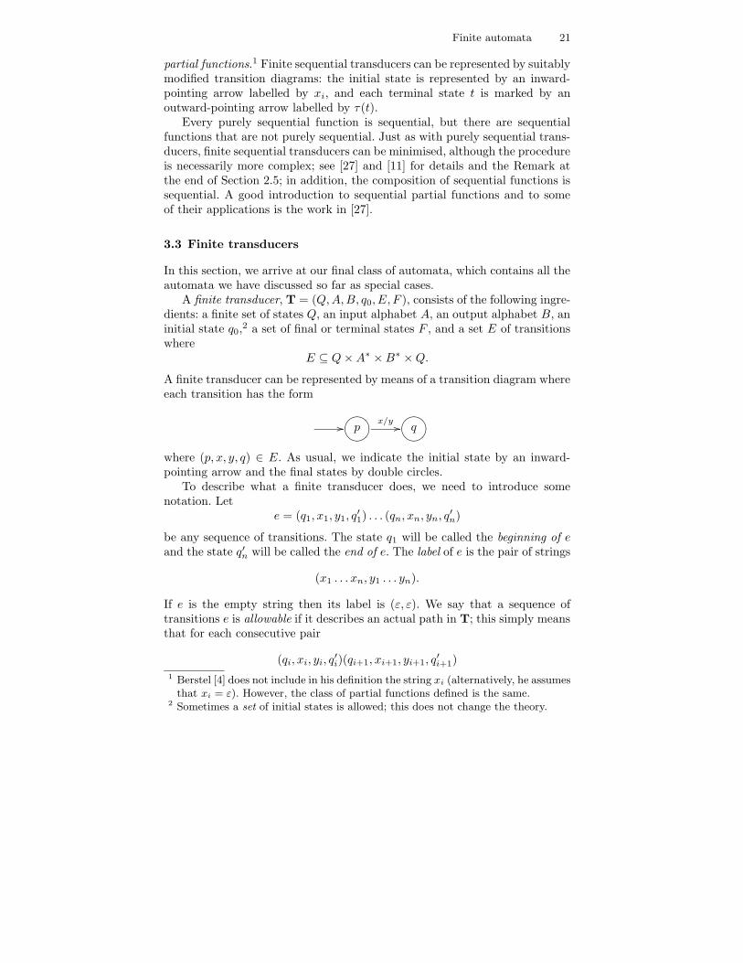
A finite transducer can be represented by means of a transition diagram whereeach transition has the form

// GFED@ABCpx/y // GFED@ABCq

where (p, x, y, q) ∈ E. As usual, we indicate the initial state by an inward-pointing arrow and the final states by double circles.

To describe what a finite transducer does, we need to introduce somenotation. Let

e = (q1, x1, y1, q′1) . . . (qn, xn, yn, q

′n)

be any sequence of transitions. The state q1 will be called the beginning of eand the state q′n will be called the end of e. The label of e is the pair of strings

(x1 . . . xn, y1 . . . yn).

If e is the empty string then its label is (ε, ε). We say that a sequence oftransitions e is allowable if it describes an actual path in T; this simply meansthat for each consecutive pair

(qi, xi, yi, q′i)(qi+1, xi+1, yi+1, q

′i+1)

1 Berstel [4] does not include in his definition the string xi (alternatively, he assumesthat xi = ε). However, the class of partial functions defined is the same.

2 Sometimes a set of initial states is allowed; this does not change the theory.

22 M. V. Lawson

in e we have that q′i = qi+1. An allowable sequence e is said to be successful ifit begins at the initial state and ends at a terminal state. Define the relation

R(T) = {(x, y) ∈ A∗ ×B∗: (x, y) is the label of a successful path in T}.

We call R(T) the relation computed by T.Observe that in determining the y ∈ B∗ such that (x, y) ∈ R(T) for a given

x, the transducer T processes the string x in the manner of an ε-acceptor.Thus we need to search for those paths in T starting at the initial state andending at a terminal state such that the sequence of labels (a1, b1), . . . , (an, bn)encountered has the property that the concatenation a1 . . . an is equal to xwhere some of the ai may well be ε.

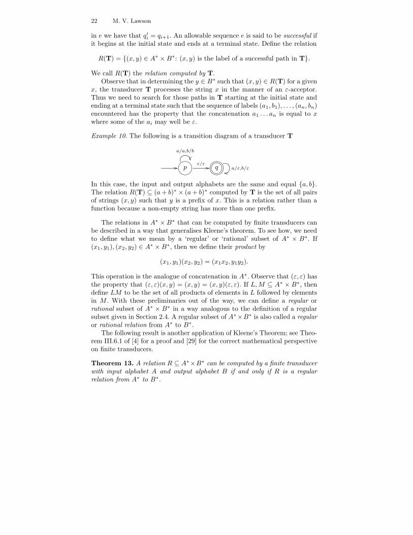
Example 10. The following is a transition diagram of a transducer T

// GFED@ABCp

a/a,b/b

±±ε/ε // GFED@ABC?>=<89:;q a/ε,b/ε

ll

In this case, the input and output alphabets are the same and equal {a, b}.The relation R(T) ⊆ (a+ b)∗ × (a+ b)∗ computed by T is the set of all pairsof strings (x, y) such that y is a prefix of x. This is a relation rather than afunction because a non-empty string has more than one prefix.

The relations in A∗ ×B∗ that can be computed by finite transducers canbe described in a way that generalises Kleene’s theorem. To see how, we needto define what we mean by a ‘regular’ or ‘rational’ subset of A∗ × B∗. If(x1, y1), (x2, y2) ∈ A

∗ ×B∗, then we define their product by

(x1, y1)(x2, y2) = (x1x2, y1y2).

This operation is the analogue of concatenation in A∗. Observe that (ε, ε) hasthe property that (ε, ε)(x, y) = (x, y) = (x, y)(ε, ε). If L,M ⊆ A∗ × B∗, thendefine LM to be the set of all products of elements in L followed by elementsin M . With these preliminaries out of the way, we can define a regular orrational subset of A∗ × B∗ in a way analogous to the definition of a regularsubset given in Section 2.4. A regular subset of A∗×B∗ is also called a regularor rational relation from A∗ to B∗.

The following result is another application of Kleene’s Theorem; see Theo-rem III.6.1 of [4] for a proof and [29] for the correct mathematical perspectiveon finite transducers.

Theorem 13. A relation R ⊆ A∗×B∗ can be computed by a finite transducerwith input alphabet A and output alphabet B if and only if R is a regularrelation from A∗ to B∗.

Finite automata 23

In the Introduction, I indicated that there were simple computations thatfinite transducers could not do. A good example is that of reversing a string;see Exercise III.3.2 of [4].

The theory of finite transducers is more complex than that of finite accep-tors. In what follows, I just touch on some of the key points.

The following is proved as Theorem III.4.4 of [4].

Theorem 14. Let A,B,C be finite alphabets. Let R be a regular relation fromA∗ to B∗ and let R′ be a regular relation from B∗ to C∗. Then R′ ◦ R is aregular relation from A∗ to C∗, where (a, c) ∈ R′ ◦ R iff there exists b ∈ B∗

such that (a, b) ∈ R′ and (b, c) ∈ R.

Let R be a regular relation from A∗ to B∗. Given a string x ∈ A∗, theremay be no strings y such that (x, y) ∈ R; there might be exactly one suchstring y; or they might be many such strings y. If a relation R from A∗ to B∗

has the property that for each x ∈ A∗ there is at most one element y ∈ B∗

such that (x, y) ∈ R, then R can be regarded as a partial function from A∗ toB∗. Such a function is called a regular or rational partial function.

It is important to remember that a regular relation that is not a regu-lar partial function is not, in some sense, deficient; there are many situationswhere it would be unrealistic to expect a partial function. For example, in nat-ural language processing, regular relations that are not partial functions canbe used to model ambiguity of various kinds. However, regular partial func-tions are easier to handle. For example, there is an algorithm that will deter-mine whether two regular partial functions are equal or not (Corollary IV.1.3[4]), whereas there is no such algorithm for arbitrary regular relations (Theo-rem III.8.4(iii) [4]). Classes of regular relations sharing some of the advantagesof sequential partial functions are described in [1] and [23].

Theorem 15. There is an algorithm that will determine whether the relationcomputed by a finite transducer is a partial function or not.

This was first proved by Schutzenberger [32], and a more recent paper [3]also discusses this question.

Both left and right purely sequential functions are examples of regularpartial functions, and there is an interesting relationship between arbitraryregular partial functions and the left and right purely sequential ones. Thefollowing is proved as Theorem IV.5.2 of [4].

Theorem 16. Let f : A∗ → B∗ be a partial function such that f(ε) = ε. Thenf is regular if and only if there is an alphabet C and a left purely sequentialpartial function fL: A

∗ → C∗ and a right purely sequential partial functionfR: C

∗ → B∗ such that f = fR ◦ fL.

The idea behind the theorem is that to compute f(x) we can first processx from left to right and then from right to left. Minimisation of machines that

24 M. V. Lawson

compute regular partial functions is more complex and less clear-cut than forthe sequential ones; see [28] for some work in this direction.

The sequential functions are also regular partial functions. The followingdefinition is needed to characterise them. Let x and y be two strings over thesame alphabet. We denote by x∧ y the longest common prefix of x and y. Wedefine the prefix distance between x and y by

d(x, y) = |x|+ |y| − 2|x ∧ y|.

In other words, if x = ux′ and y = uy′, where u = x ∧ y, then d(x, y) =|x′|+ |y′|. A partial function f : A∗ → B∗ is said to have bounded variation iffor each natural number n there exists a natural number N such that, for allstrings x, y ∈ A∗,

if d(x, y) ≤ n then d(f(x), f(y)) ≤ N .

Theorem 17. Every sequential function is regular. In particular, the sequen-tial functions are precisely the regular partial functions with bounded variation.

The proof of the second claim in the above theorem was first given byChoffrut [10]. Both proofs can be found in [4] (respectively, Proposition IV.2.4and Theorem IV.2.7).

Theorem 18. There is an algorithm that will determine whether a finitetransducer computes a sequential function.

This was first proved by Choffrut [10], and more recent papers that discussthis question are [2] and [3].

Finite transducers were introduced in [13] and, as we have seen, form ageneral framework containing the purely sequential and sequential transduc-ers.

4 Final Remarks

In this section, I would like to touch on some of the practical reasons forusing finite transducers. But first, I need to deal with the obvious objectionto using them: that they cannot implement all algorithms, because they donot constitute a universal programming language. However, it is the very lackof ambition of finite transducers that leads to their virtues: we can say moreabout them, and what we can say can be used to help us design programsusing them. The manipulation of programs written in universal programminglanguages, on the other hand, is far more complex. In addition:

• Not all problems require for their solution the full weight of a universalprogramming language — if we can solve them using finite transducersthen the benefits described below will follow.

Finite automata 25

• Even if the full solution of a problem does fall outside the scope of finitetransducers, the cases of the problem that are of practical interest maywell be described by finite transducers. Failing that, partial or approximatesolutions that can be described by finite transducers may be acceptablefor certain purposes.

• It is one of the goals of science to understand the nature of problems. If aproblem can be solved by a finite transducer then we have learnt somethingnon-trivial about the nature of that problem.

The benefits of finite transducers are particularly striking in the case offinite acceptors:

• Finite acceptors provide a way to describe potentially infinite languagesin finite ways.

• Determining whether a string is accepted or rejected by a deterministicacceptor is linear in the length of the string.

• Acceptors can be both determinised and minimised.

The important point to bear in mind is that languages are interesting becausethey can be used to encode structures of many kinds. An example from math-ematics may be instructive. A relational structure is a set equipped with afinite collection of relations of different arities. For example, a set equippedwith a single binary relation is just a graph with at most one edge joining anytwo vertices. We say that a relational structure is automatic if the elementsof the set can be encoded by means of strings from a regular language, andif each of the n-ary relations of the structure can be encoded by means of anacceptor. Encoding n-ary relations as languages requires a way of encodingn-tuples of strings as single strings, but this is easy and the details are notimportant; see [19] for the complete definition and [8] for a technical analy-sis of automatic structures from a logical point of view. Minimisation meansthat encoded structures can be compressed with no loss of information. Nowthere are many ways of compressing data, but acceptors provide an additionaladvantage: they come with a built-in search capability. The benefits of usingfinite acceptors generalise readily to finite sequential transducers.

There is a final point that is worth noting. Theorem 14 tells us that com-posing a sequence of finite transducers results in another finite transducer.This can be turned around and used as a design method; rather than try-ing to construct a finite transducer in one go, we can try to design it as thecomposition of a sequence of simpler finite transducers.

The books [18, 20, 31] although dealing with natural language processingcontain chapters that may well provide inspiration for applications of finitetransducers to other domains.

Acknowledgements It is a pleasure to thank a number of people who helpedin the preparation of this article.

26 M. V. Lawson

Dr Karin Haenelt of the Fraunhofer Gesellschaft, Darmstadt, provided con-siderable insight into the applications of finite transducers in natural languageprocessing which contributed in formulating Section 4.

Dr Jean-Eric Pin, director for research of CNRS, made a number of sug-gestions including the choice of terminology and the need to clarify what ismeant by the notion of minimisation.

Dr Anne Heyworth of the University of Leicester made a number of usefultextual comments as well as providing the automata diagrams.

Prof John Fountain and Dr Victoria Gould of the University of York madea number of helpful comments on the text.

My thoughts on the role of finite transducers in information processingwere concentrated by a report I wrote for DSTL in July 2003 (Contract num-ber RD026-00403) in collaboration with Peter L. Grainger of DSTL.

Any errors remaining are the sole responsibility of the author.

References

1. C. Allauzen and M. Mohri, Finitely subsequential transducers, Interna-

tional J. Foundations Comp. Sci. 14 (2003), 983–994.2. M.-P. Beal and O. Carton, Determinization of transducers over finite and infinite

words, Theoret. Comput. Sci. 289 (2002), 225–251.3. M.-P. Beal, O. Carton, C. Prieur, and J. Sakarovitch, Squaring transducers,

Theoret. Comput. Sci. 292 (2003), 45–63.4. J. Berstel, Transductions and Context-free Languages, B.G. Teubner, Stuttgart,

1979.5. J. Berstel and J.-E. Pin, Local languages and the Berry-Sethi algorithm, Theo-

ret. Comput. Sci. 155 (1996), 439–446.6. J. Berstel and D. Perrin, Algorithms on words, in Applied Combinatorics on

Words (editor M. Lothaire), in preparation, 2004.7. A. Bruggemann-Klein, Regular expressions into finite automata, Lecture Notes

in Computer Science 583 (1992), 87–98.8. A. Blumensath, Automatic structures, Diploma Thesis, Rheinisch-Westfalische

Technische Hochschule Aachen, Germany, 1999.9. J. Carroll and D. Long, Theory of Finite Automata, Prentice-Hall, Englewood

Cliff, NJ, 1989.10. Ch. Choffrut, Une caracterisation des fonctions sequentielles et des fonctions

sous-sequentielles en tant que relations rationelles, Theoret. Comput. Sci. 5

(1977), 325–337.11. Ch. Choffrut, Minimizing subsequential transducers: a survey, Theoret. Com-

put. Sci. 292 (2003), 131–143.12. S. Eilenberg, Automata, Languages, and Machines, Volume A, Academic Press,

New York, 1974.13. C. C. Elgot and J. E. Mezei, On relations defined by generalized finite automata,

IBM J. Res. Develop. 9 (1965), 47–65.14. J. E. F. Friedl, Mastering regular expressions, O’Reilly, Sebastopol, CA, 2002.15. S. Ginsburg and G. F. Rose, A characterization of machine mappings,

Can. J. Math. 18 (1966), 381–388.

Finite automata 27

16. J. E. Hopcroft and J. D. Ullman, Introduction to Automata Theory, Languages,

and Computation, Addison-Wesley, Reading, MA, 1979.17. J. E. Hopcroft, R. Motwani, and J. D. Ullman, Introduction to Automata Theory,

Languages, and Computation, 2nd Edition, Addison-Wesley, Reading, MA, 2001.18. D. Jurafsky and J. H. Martin, Speech and Language Processing, Prentice-Hall,

Englewood Cliff, NJ, 2000.19. B. Khoussainov and A. Nerode, Automatic presentations of structures, Lecture

Notes in Computer Science 960 (1995), 367–392.20. A. Kornai (editor), Extended Finite State Models of Language, Cambridge Uni-

versity Press, London, 1999.21. E. Laporte, Symbolic natural language processing, in Applied Combinatorics on

Words (editor M. Lothaire), in preparation, 2004.22. M. V. Lawson, Finite Automata, CRC Press, Boca Raton, FL, 2003.23. M. Mohri, Finite-state transducers in language and speech processing, Com-

put. Linguistics 23 (1997), 269–311.24. M. Pelletier and J. Sakarovitch, On the representation of finite deterministic

2-tape automata, Theoret. Comput. Sci. 225 (1999), 1–63.25. D. Perrin, Finite automata, in Handbook of Theoretical Computer Science, Vol-

ume B (editor J. Van Leeuwen), Elsevier, Amsterdam, 1990, 1–57.26. D. Perrin and J. E. Pin, Infinite Words, Elsevier, Amsterdam, 2004.27. Ch. Reutenauer, Subsequential functions: characterizations, minimization, ex-

amples, Lecture Notes in Computer Science 464 (1990), 62–79.28. Ch. Reutenauer and M.-P. Schutzenberger, Minimization of rational word func-

tions, Siam. J. Comput. 20 (1991), 669–685.29. J. Sakarovitch, Kleene’s theorem revisited, Lecture Notes in Computer Science

281 (1987), 39–50.30. J. Sakarovitch, Elements de Theorie des Automates, Vuibert, Paris, 2003.31. E. Roche and Y. Schabes (editors), Finite-State Language Processing, The MIT

Press, 1997.32. M.-P. Schutzenberger, Sur les relations rationelles, in Automata theory and for-

mal languages (editor H. Brakhage), Lecture Notes in Computer Science 33

(1975), 209–213.33. M.-P. Schutzenberger, Sur une variante des fonctions sequentielles, Theo-

ret. Comput. Sci. 4 (1977), 47–57.34. B. W. Watson, Implementing and using finite automata toolkits, in Extended

Finite State Models of Language (editor A. Kornai), Cambridge University Press,London, 1999, 19–36.

35. Sheng Yu, Regular languages, in Handbook of Formal Languages, Volume 1 (ed-itors G. Rozenberg and A. Salomaa), Springer-Verlag, Berlin, 1997, 41–110.