finding structural similarity in time series data using …jessica/lin_bop_ssdbm.pdf · ·...

M. Winslett (Ed.): SSDBM 2009, LNCS 5566, pp. 461–477, 2009. © Springer-Verlag Berlin Heidelberg 2009

Finding Structural Similarity in Time Series Data Using Bag-of-Patterns Representation

Jessica Lin and Yuan Li

Computer Science Department George Mason University

[email protected], [email protected]

Abstract. For more than one decade, time series similarity search has been given a great deal of attention by data mining researchers. As a result, many time series representations and distance measures have been proposed. How-ever, most existing work on time series similarity search focuses on finding shape-based similarity. While some of the existing approaches work well for short time series data, they typically fail to produce satisfactory results when the sequence is long. For long sequences, it is more appropriate to consider the similarity based on the higher-level structures. In this work, we present a histo-gram-based representation for time series data, similar to the “bag of words” approach that is widely accepted by the text mining and information retrieval communities. We show that our approach outperforms the existing methods in clustering, classification, and anomaly detection on several real datasets.

Keywords: Data mining, Time series, Similarity Search.

1 Introduction

Time series similarity search has been a major research topic for time series data mining for more than one decade. As a result, many time series representations and distance measures have been proposed [3, 6, 12, 15, 17, 19]. There are two kinds of similarities: shape-based similarity and structure-based similarity [13]. The former determines the similarity of two datasets by comparing their local patterns, whereas the latter determines the similarity by comparing their global structures. Most existing approaches focus on finding shape-based similarity. While some of these approaches work well for short time series data, they typically fail to produce satisfactory results when the sequence is long. To understand the need for a higher-level, structure-based similarity measure for long time series data, consider the scenario for textual data. If we are to compare two strings, we can use the string edit distance to compute their similarity. However, if we want to compare two documents, we typically do not com-pare them on the word-to-word basis. Instead, it is more meaningful to use a higher-level representation that can capture the structure or semantic of the document. Be-low, we describe the two types of similarities in more detail [13].

Given two sequences A and B, shape-based similarity determines how similar these two datasets are based on local comparisons. The most well-known distance measure in data mining literature is the Euclidean distance, for which sequences are

462 J. Lin and Y. Li

aligned in the point-to-point fashion, i.e. the ith point in sequence A is matched with the ith point in sequence B. While Euclidean distance works well in general, it does not always produce accurate results when data is shifted, even slightly, along the time axis. For example, the top and bottom sequences in Figure 1 appear to have similar shapes. In fact, the sequence below is the shifted version of the sequence above. However, the slight shifts along the time axis will result in a large distance between the two sequences.

Another distance measure, Dynamic Time Warping (DTW) [12, 24], overcomes this limitation by using dynamic programming technique to determine the best alignment that will produce the optimal distance. The parameter, warping length, determines how much warping is allowed to find the best alignment. A large warping window causes the search to become prohibitively expensive, as well as possibly allowing meaningless matching between points that are far apart. On the other hand, a small window might prevent us from finding the best solution. Euclidean distance can be seen as a special case of DTW, where there is no warping allowed. Figure 1 dem-onstrates the difference between the two distance measures. Note that with Euclidean distance, the dips and peaks in the sequences are mis-aligned and therefore not matched, whereas with DTW, the dips and peaks are aligned with their corresponding points from the other sequence. While DTW is a more robust distance measure than Euclidean distance, it is also a lot more computationally intensive. Keogh [12] pro-posed an indexing scheme for DTW that allows faster retrieval. Nevertheless, DTW is still at least several orders slower than Euclidean distance.

Fig. 1. (Left) Alignment for Euclidean distance between two sequence data. (Right) Alignment for Dynamic Time Warping distance between two sequence data.

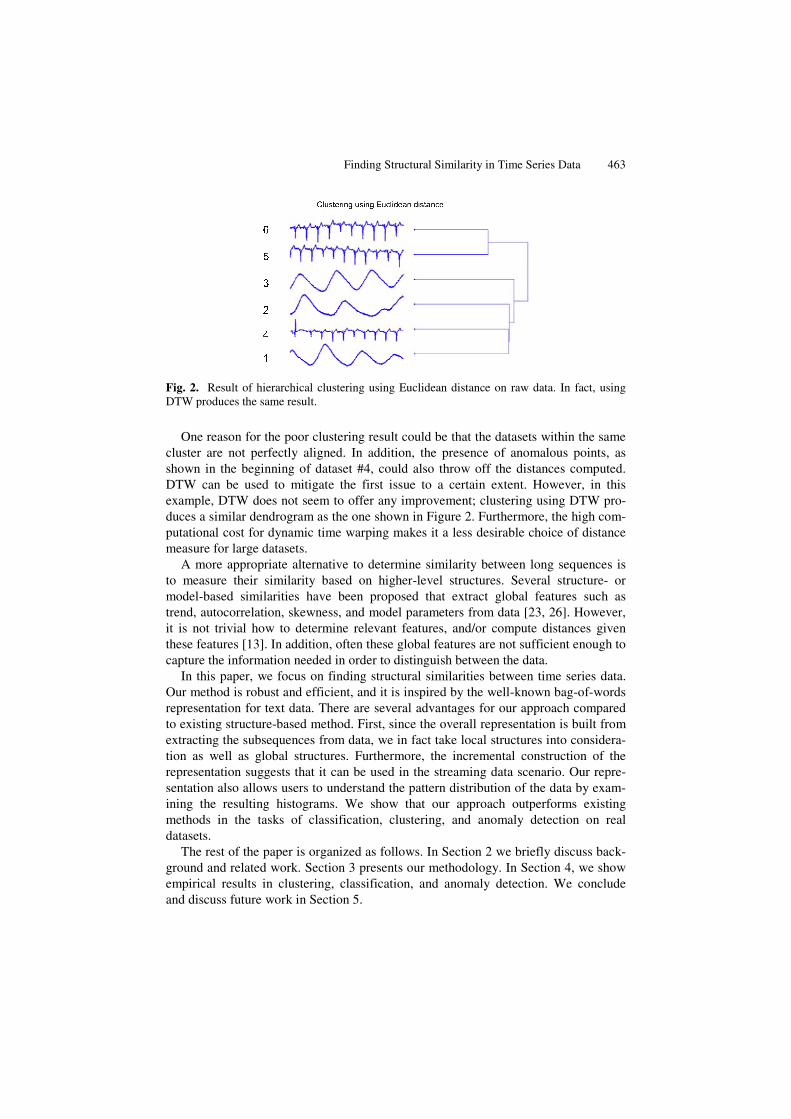
Shape-based similarities work well for short time series or subsequences; however, for long sequence data, they produce poor results. To illustrate this, we extracted subsequences of length 682 from six different records on PhysioNet [10], an online medical archive containing digital recordings of physiological signals. The first three datasets (numbered #1 ~ #3) are measurements on respiratory rates, and the last three datasets (#4 ~ #6) are electrocardiograms (ECGs). As we can clearly see in Figure 2, these two types of vital signs have very different structures. Visually we can separate the two classes with no difficulty. However, if we cluster them using Euclidean dis-tance as the distance measure, the result is disappointing. Figure 2 shows the hierar-chical clustering result using Euclidean distance. The dendrogram illustrates that while datasets #5 and #6 are correctly clustered (i.e. they share a common parent node), the rest are not.

Finding Structural Similarity in Time Series Data 463

Fig. 2. Result of hierarchical clustering using Euclidean distance on raw data. In fact, using DTW produces the same result.

One reason for the poor clustering result could be that the datasets within the same cluster are not perfectly aligned. In addition, the presence of anomalous points, as shown in the beginning of dataset #4, could also throw off the distances computed. DTW can be used to mitigate the first issue to a certain extent. However, in this example, DTW does not seem to offer any improvement; clustering using DTW pro-duces a similar dendrogram as the one shown in Figure 2. Furthermore, the high com-putational cost for dynamic time warping makes it a less desirable choice of distance measure for large datasets.

A more appropriate alternative to determine similarity between long sequences is to measure their similarity based on higher-level structures. Several structure- or model-based similarities have been proposed that extract global features such as trend, autocorrelation, skewness, and model parameters from data [23, 26]. However, it is not trivial how to determine relevant features, and/or compute distances given these features [13]. In addition, often these global features are not sufficient enough to capture the information needed in order to distinguish between the data.

In this paper, we focus on finding structural similarities between time series data. Our method is robust and efficient, and it is inspired by the well-known bag-of-words representation for text data. There are several advantages for our approach compared to existing structure-based method. First, since the overall representation is built from extracting the subsequences from data, we in fact take local structures into considera-tion as well as global structures. Furthermore, the incremental construction of the representation suggests that it can be used in the streaming data scenario. Our repre-sentation also allows users to understand the pattern distribution of the data by exam-ining the resulting histograms. We show that our approach outperforms existing methods in the tasks of classification, clustering, and anomaly detection on real datasets.

The rest of the paper is organized as follows. In Section 2 we briefly discuss back-ground and related work. Section 3 presents our methodology. In Section 4, we show empirical results in clustering, classification, and anomaly detection. We conclude and discuss future work in Section 5.


2 Background and Related Work

In this section, we briefly discuss background and related work on time series similar-ity search. For concreteness, we begin with a definition of time series:

Definition 1. Time Series: A time series T = t1,…,tp is an ordered set of p real-valued variables.

Some distance measure Dist(A,B) needs to be defined in order to determine the simi-larity between time series objects A and B.

Definition 2. Distance: Dist is a function that has A and B as inputs and returns a nonnegative value R, which is said to be the distance from A to B.

Each time series is normalized to have a mean of zero and a standard deviation of one before calling the distance function, since it is well understood that in virtually all settings, it is meaningless to compare time series with different offsets and amplitudes [15].

As mentioned, Euclidean distance and Dynamic Time Warping are among the most commonly used distance measures for time series. For this reason, we will use Euclidean distance for our new representation, and compare the results with using Euclidean distance and Dynamic Time Warping on raw data.

In addition to comparing with well-known distance measures on the raw data, we also demonstrate that our method outperforms existing time series representations such as Discrete Fourier Transform (DFT) [1]. DFT approximates the signal with a linear combination of basis functions, and its coefficients represent global contribution of the signal. Another well-known representation is Discrete Wavelet Transform (DWT) [3]. Wavelets are mathematical functions that represent data or other functions in terms of the averages and differences of a prototype function, called the analyzing or mother wavelet. Contrary to DFT, wavelets are localized in time. Nevertheless, past studies have shown that DFT and DWT have similar performance in terms of accuracy [15].

While there have been dozens of representations and distance measures proposed for time series shape-based similarity, there is relatively little work on finding structure-based similarity. Deng et al [4] proposed learning ARMA model on the time series, and using the model coefficients as the feature. This approach has an obvious limitation on the characteristics of input data. Ge and Smyth [8] proposed a deformable Markov Model template for temporal pattern matching, in which the data is converted to a piecewise linear model. However, this approach requires many parameters. Nanopoulos et al [23] proposed extracting statistical features of time series such as skewness, mean, variance, and kurtosis, and classifying the data using multi-layer perceptron (MLP) neural network.

Recently, Keogh et al. [16] proposed a compression-based distance measure that compares the co-compressibility between datasets. Motivated by Kolmogorov Complexity [16, 19] and promising results shown in similar work in bioinformatics and computational theory, the authors devised a new dissimilarity measure called CDM (Compression-based Dissimilarity Measure). Given two datasets (strings) x and y, their compression-based dissimilarity measure can be formulated as follows:


CDM(x,y) = C(xy)C(x) + C(y)

where C(xy) is the compressed size of the concatenated string x+y, C(x) and C(y) are the compressed sizes of the string x and y, respectively. In their paper, the authors show superior results compared to other existing structural similarity approaches. For this reason, we will compare our method with CDM, the best structure-based (dis)similarity measure reported. We will show that our approach is highly competi-tive, with several additional advantages over existing methods.

3 Finding Structural Similarity

We propose a histogram-based similarity measure, using a representation similar to the one widely used for text data. In the Vector Space Model [25], each document can be represented as a vector in the vector space. Each dimension of the vector corre-sponds to one word in the vocabulary, and the value of each component is the (rela-tive) frequency of occurrences for the corresponding word in the document. As a result, an p-by-q term-to-document matrix X is constructed, where p is the number of unique terms in the text collection, q is the number of documents, and each element X(i,j) is the frequency of the ith word occurring in the jth document.

This “bag of words” representation works well for documents. It is able to capture the structure or topic of a document, without knowing the exact locations or orderings of the word appearances. This suggests that we might be able to represent time series data in a similar fashion, i.e. as a combination of patterns from a finite set of patterns.

There are two challenges if we wish to represent time series data as a “bag of patterns.” The first challenge concerns with the definition and construction of the patterns “vocabulary.” The second challenge comes from the fact that time series data are composed of consecutive data points. There is no clear “delimiters” between patterns. Fortunately, a symbolic representation for time series called SAX (Symbolic Aggregate approXimation) [20], previously developed by the current author and now a widely used discretization method, provides solutions to these challenges. The intuition is to convert the time series into a set of SAX words, and then construct a word-sequence matrix (analogous to the term-document matrix for text data) using these SAX words. In the next section, we briefly discuss how SAX converts time series data into strings.

3.1 Symbolic Aggregate Approximation

Given a time series of length n, SAX produces a lower dimensional representation of a time series by transforming the original data into symbolic words. Two parameters are used to specify the size of the alphabet to use (i.e. α) and the size of the words to produce (i.e. w). The algorithm begins by using a normalized version of the data and creating a Piecewise Aggregate Approximation (PAA). PAA reduces the dimensionality of a time series by transforming the original representation into a user defined number (i.e. w, typically w << n) of equal segments. The segment values are determined by calculating the mean of the data points in that segment. The PAA values are then transformed into symbols by using a breakpoint table. The breakpoints


in the breakpoint table are defined such that all the regions have approximately equi-probability based on a Gaussian distribution1. These breakpoints may be determined by looking them up in a statistical table. For example, Table 1 gives the breakpoints for values of α from 3 to 5.

Table 1. A lookup table that contains the breakpoints that divides a Gaussian distribution into an arbitrary number (from 3 to 5) of equiprobable regions

βi a 3 4 5

β1 -0.43 -0.67 -0.84

β2 0.43 0 -0.25

β3 0.67 0.25

β4 0.84

Figure 3 summarizes how a time series is converted to PAA and then symbols, with parameters α = 3 and w = 8.

Fig. 3. Example of SAX for a time series, with parameters α = 3 and w = 8. The time series above is transformed to the string cbccbaab, and the dimensionality is reduced from 128 to 8.

3.2 Bag-of-Words Representation for Time Series

Our algorithm works as follows. For each time series, we use a sliding window and extract every possible subsequence of length n (a user-defined parameter). Each subsequence is normalized to have mean of zero and standard deviation of one before it is converted to a SAX string. As a result, we obtain a set of strings, each of which corresponds to a subsequence in the time series. As noted in [20], given a subsequence Si, it is likely to be very similar to its neighboring subsequences, Si-1 and Si+1 (i.e. those that start one point to the left, and one point to the right of Si), especially if Si is in the smooth region of the time series. These subsequences are called trivial matches of Si. To avoid over-counting these trivial matches as true 1 The Gaussian assumption is the default, since in [20] the authors discover that most short time

series subsequences follow the Gaussian distribution. However, the breakpoints can be ad-justed based on the actual distribution of the data.


patterns, we need to perform numerosity reduction. Since SAX preserves the general shape of the sequence, in some cases we might see that multiple consecutive subsequences are mapped to the same string. In that case, we record only the first occurrence of the string, and ignore the rest until we encounter a string that is different. In other words, for each group of consecutive identical strings, we record only the first occurrence and count this group of occurrences only once.

Once we obtain the set of strings for each time series dataset, we can construct the word-sequence matrix. Given α and w as the parameters for SAX, we know the size of our entire collection of possible SAX strings, or our “dictionary.” There are αw possible SAX words. For example, for α = 4 and w = 4, our dictionary size is only 256. Clearly, the size of the dictionary increases exponentially with the increase of w. Experimental results in previous work [20] indicate that the choice of α does not critically affect the performance. Typically, a value of 3 or 4 works well for most time series datasets. In this paper, we choose α = 4.

Having fixed α, we now have to determine the value for w. While the best choice of w is data-dependent, generally speaking, time series with smooth patterns can be described with a small w, and those with rapidly changing patterns prefer large w to capture the critical changes. We choose w = 6~8 for our experiments, with sliding window length of 100~300.

With α = 4 and w = 8, the resulting dictionary size is αw = 48 = 65536, which is still quite large. However, as is the case for text documents, the matrix is likely to be sparse. Therefore, we can eliminate the words that never occur in the data, and/or store the matrix in a compressed format such as the Compressed Column Storage (CCS) format [5]. In our experiments, we find that only about 10% of all words have some subsequence mapped to it.

The construction of the temporal “bag of patterns” matrix is straightforward. The matrix M is a word-sequence matrix, where each row i denotes a SAX word (i.e. a pattern) from the dictionary; each column j denotes a time series dataset; and each Mi,j

stores the frequency of word i occurring in time series j. Within each matrix cell Mi,j, we can also store a list of pointers to the subsequence in time series j (typically on disk) that are mapped to word i. The lists of pointers will enable us to perform subsequence matching. However, since we are focused on finding structural similarities between time series data, we will contend ourselves with storing just the word frequency in the matrix for now. We call this new representation BOP (Bag of Patterns).

The matrix provides a summary of time series data in terms of the frequency of occurrence for each pattern. Once we build the matrix M, we can then use any applicable distance measures or dimensionality reduction techniques to computes the similarity between different time series datasets. Figure 4 shows a visual example of this representation. Like the bag-of-words representation for documents, the orderings of words are lost. However, for long time series data, this level of details is exactly the reason why conventional shaped-based approaches do not work well. As our experiments demonstrate, BOP produces very good results even without knowing the ordering of the patterns.


Fig. 4. A visual example of the bag-of-patterns representation for time series. Each row de-notes a SAX word, and each column denotes a time series data. We could also store, within each cell, pointers to corresponding subsequences.

4 Empirical Evaluation

In this section, we present empirical evaluation of our method on clustering, classifi-cation, and anomaly detection.

4.1 Clustering

For this part of experiments, we demonstrate the effectiveness of our approach in clustering. We show that our representation out-perform existing approaches and produce more accurate clustering results. 4.1.1 Hierarchical Clustering One of the most widely used clustering approaches is hierarchical clustering [11]. Hierarchical clustering computes pairwise distances of the objects (or groups of ob-jects) and produces a nested hierarchy of the clusters. It has several advantages over other clustering methods. More specifically, it offers great visualization power with the hierarchy of clusters, and it requires no input parameters. However, its intensive computational complexity makes it infeasible for large datasets.

In Figure 2, we showed a simple example on hierarchical clustering where both Euclidean Distance and Dynamic Time Warping on the raw data fail to find the correct clusters. In this part of experiment, as a sanity check, we show the clustering result using BOP to represent the time series datasets. We use Euclidean distance to compute the similarity between the histograms (i.e. the column vectors). Figure 5 shows the resulting dendrogram. Note we are now clustering on the transformed time series, or the histogram of the patterns. For clarity, we also plot the original, corresponding time series to the left of the histograms. We can see


Fig. 5. New clustering result on the same data shown in Figure 2. This time, we use our histo-gram-based, bag-of-patterns approach, and combine it with Euclidean distance. The two clus-ters are well separated.

Fig. 6. Clustering result using Euclidean distance on the raw data. Only three pairs of data are cleanly clustered together.

clearly from the histograms that the time series clustered together share similar pattern distribution.

While the example shown above gives us a first indication that our approach can find clusters while shape-based approaches cannot, with only six datasets, the example is too small and contrived to offer any conclusive insight. Therefore, we perform more hierarchical clustering experiments on larger datasets. We compare our approach with the following methods: (1) CDM proposed by Keogh et al [16], (2) Euclidean distance on raw time series, (2) Dynamic Time Warping on raw time series, and (4) Euclidean distance on DFT coefficients.

Similar to the experimental setting in [16], we selected 13 pairs of datasets across different domains, with diverse structures from UCR Time Series Archive [14]. Although our method does not require the input time series to have the same length, for simplicity, we keep each dataset at length 1000. For Dynamic Time Warping,


however, since it is costly to compute, we reduce the time series length to 250 by systematic sampling.

Figure 62 shows the dendrogram produced by hierarchical clustering using Euclidean distance on the raw data. We can see that out of 13 pairs of datasets, only 3 pairs are successfully clustered together.

As illustrated in Figure 7, DTW shows improvement over Euclidean distance and successfully clusters 10 pairs of dataset. Perhaps the clustering results for DTW would have been better if we used the entire dataset. However, its prohibitive time complexity makes it an unrealistic choice of distance measure for large datasets. Even at the reduced length, DTW took 156 times longer than our approach on the whole dataset.

Fig. 7. Clustering result using Dynamic Time Warping on the raw data. The result is better than Euclidean: 10 pairs of data are cleanly clustered together.

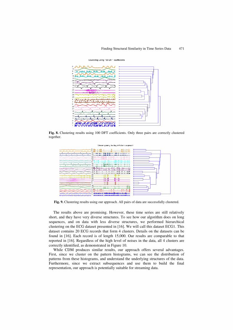
Next, we convert the time series by DFT, and cluster the data on the DFT coefficients. One of the advantages of DFT is that it offers dimensionality reduction. As demonstrated in [1], most “energy” concentrates on the first few DFT coefficients. Therefore, we can use only a few DFT coefficients to approximate the data, while still preserving the general shape of the data. If we use all the coefficients, then we get back the original sequence. In this experiment, we used 100 coefficients (compared to 1000 data points in the raw data). Similar to using the raw data, only 3 pairs of data are cleanly clustered. Figure 8 shows the result.

Figure 9 shows the clustering result produced by our BOP approach. Again, the histograms for the bag-of-patterns are shown in the middle of the figure. As we can see, all 13 pairs are successfully clustered.

2 The figures are best viewed in color.


Fig. 8. Clustering results using 100 DFT coefficients. Only three pairs are correctly clustered together.

Fig. 9. Clustering results using our approach. All pairs of data are successfully clustered.

The results above are promising. However, these time series are still relatively short, and they have very diverse structures. To see how our algorithm does on long sequences, and on data with less diverse structures, we performed hierarchical clustering on the ECG dataset presented in [16]. We will call this dataset ECG1. This dataset contains 20 ECG records that form 4 clusters. Details on the datasets can be found in [16]. Each record is of length 15,000. Our results are comparable to that reported in [16]. Regardless of the high level of noises in the data, all 4 clusters are correctly identified, as demonstrated in Figure 10.

While CDM produces similar results, our approach offers several advantages. First, since we cluster on the pattern histograms, we can see the distribution of patterns from these histograms, and understand the underlying structures of the data. Furthermore, since we extract subsequences and use them to build the final representation, our approach is potentially suitable for streaming data.


Fig. 10. Clustering result on 20 ECG datasets, using our bag-of-patterns approach. Each record is 15,000 points long.

Next, we compare our results with the three other methods that we mentioned. Figure 11 shows the clustering results using Euclidean distance on the raw data. Only 9 out of 20 datasets are clustered correctly.

Fig. 11. Clustering result on raw ECG1 data using Euclidean Distance. Only 9 datasets are correctly clustered (#11, #12, #14, #15, #16-#20)

When we repeat the experiment using DTW, we had to sample down the data (20:1), due to its high computational cost. Our machine simply could not handle it. With DTW on the shorter datasets, the result is similar to that of Euclidean distance on the full datasets. To show that this poor result is not just due to the loss of data from sampling, we re-ran the experiment using our BOP representation on the sampled, shorter datasets, and obtained the same result as shown in Figure 10.

For the final comparison, we convert the time series to DFT coefficients, and cluster the data on the coefficients. Similar to Euclidean Distance on the raw data, only 8 datasets are clustered correctly. We also tried different resolutions (100-1000 coefficients), but obtained poor results regardless of the resolution. The result is shown in Figure 12.


Fig. 12. Clustering result on ECG1 data using 1000 DFT coefficients

4.1.2 Partitional Clustering Although hierarchical clustering is a good sanity check from its visualization power, it has limited utility due to its poor scalability. The most commonly used data mining clustering algorithm is k-means [2, 22, 21]. We performed k-means using the Euclidean distance on the raw data, and on our bag-of-patterns representation. The basic intuition behind k-means (and in general, iterative refinement algorithms) is the continuous reassignment of objects into different clusters, so that the intra-cluster distance is minimized.

We performed k-means using the Euclidean distance on the raw data, and on our histogram-based representation. CDM is not included in this experiment, as it’s unclear how to define the centroid of a cluster [16].

For this experiment, we extracted 250 records from the PhysioNet archive. Each record contains 2048 points. These records are extracted from various databases containing different vital signs, or patients with different heart conditions. We separated the records into 5 classes, and labeled them according to the databases that they are extracted from. We will call this dataset ECG2. Figure 13 shows one example from each of the 5 classes in ECG2 dataset.

Fig. 13. One example from each of the 5 classes in ECG2 dataset


We ran k-means algorithm 10 times, and recorded the clustering labels obtained from the run with the smallest objective function (i.e. sum of intra-cluster distances). We then compare our cluster labels with the true labels, and compute the clustering quality using the evaluation method proposed by [7]. The evaluation method compares the similarity between two sets of cluster labels, and returns a number between 0 and 1 denoting how similar they are. Ideally, we would like the number to be as close to 1 as possible. Our approach achieves the best clustering quality (0.7133 vs. 0.4644). The results are shown in Table 2.

4.2 Classification

Classification of time series has attracted much interest from the data mining community [10, 22, 23, 24]. For the classification experiments, we will consider the most common classification algorithm, nearest neighbor classification. To demonstrate the effectiveness on 1-nearest-neighbor classification, we use the same ECG2 dataset. We use the leave-one-out cross validation, and count the number of correctly classified objects, cc. The accuracy is the ratio of cc and the total number of objects (i.e. 250). For this experiment, we also add Dynamic Time Warping (again, with reduced length). The accuracy results are show in Table 2. The improvement is astounding. For our approach, the accuracy of 0.996 means that there is only 1 misclassified object, out of 250 objects.

4.3 Discord/Anomaly Detection

In [18], a discord is defined as the data object that is the least similar to the rest of the dataset, i.e. it has the largest nearest neighbor distance. A discord can be seen as an anomaly in the data. In this section, we conduct discord/anomaly detection experiments, using our BOP representation and comparing it with Euclidean distance on the raw data. We use the same ECG2 dataset. We take one class of ECG2 data at a time (each class contains 50 ECG records), and manually insert an anomaly by randomly choosing one other ECG record that belongs to a different class. For each class, we repeat this experiment 20 times, which results in a total of 100 runs. We then compare the accuracy, or the percentage of discords found, of our representation against the raw data, both using Euclidean distance. The accuracy results are shown in Table 2.

Table 2. Accuracy of our approach on clustering, classification, and discord discovery com-pared to other methods. Our approach achieves the best accuracy for all tasks. All numbers are between 0 and 1.

Euclidean DTW Bag-of-Patterns k-means 0.4644 N/A 0.7133

NN 0.44 0.728 0.996 Discord 0.35 N/A 0.85


One of the reasons that our approach works so much better than using the raw data is that the ECG data are not at all aligned, even for datasets in the same class. Another reason is that sometimes an ECG data might contain local anomalies within the data; such anomalies can easily throw off the distances computed using the shape-based approach.

We conclude this experiment by noting that the definition of discord can be easily extended to top k-discords. Applying k-discords discovery algorithm will allow us to find both global (i.e. data that do not belong in the cluster) and local (i.e. anomalies that occur within one time series) anomalies.

5 Conclusion

Most existing work on time series similarity search focuses on finding shaped-based similarity. While these shape-based approaches work reasonably well for short time series data, the accuracy typically degrades if the sequences are long. For long time sequences, it is more appropriate to measure the similarity by looking at their higher-level structures, rather than point-to-point, local comparisons.

In this work, we proposed a histogram-based similarity measure, BOP. Similar to the bag-of-words representation for textual data, our approach counts the frequency of occurrences of each pattern in the time series. We then compare the frequencies (or the histograms) of patters in the time series to obtain a (dis)similarity measure.

Our experimental results show that our approach is superior to existing approaches in the tasks of clustering, classification, and anomaly detection. Furthermore, our approach has several advantages over existing structure-based similarity measures. Specifically, our approach considers local structures as well as global structure, by using subsequences to build our final representation. Our representation allows users to understand the pattern distribution by examining the histograms. Furthermore, our representation is suitable for streaming data, since the frequency vectors are built incrementally.

We would like to note that since our approach determines similarity based on structures of the data, the input sequences should be reasonably long, or long enough such that the structures (or lack of structures) can be meaningfully captured and summarized.

For future work, we will explore our representation on other types of data such as images. We will also try other existing distance measures such as cosine similarity, and/or devise a distance measure more suitable than Euclidean Distance.

Acknowledgments. We would like to thank Eamonn Keogh for providing the data-sets and the code for CDM.

References

1. Agrawal, R., Faloutsos, C., Swami, A.: Efficient Similarity Search in Sequence Databases. In: Proceedings of the 4th Int’l Conference on Foundations of Data Organization and Al-gorithms, Chicago, IL, October 13-15, pp. 69–84 (1993)

2. Bradley, P., Fayyad, U., Reina, C.: Scaling Clustering Algorithms to Large Databases. In: Proceedings of the 4th Int’l Conference on Knowledge Discovery and Data Mining, New York, NY, August 27-31, pp. 9–15 (1998)


3. Chan, K., Fu, A.W.: Efficient Time Series Matching by Wavelets. In: Proceedings of the 15th IEEE Int’l Conference on Data Engineering, Sydney, Australia, March 23-26, pp. 126–133 (1999)

4. Deng, K., Moore, A., Nechyba, M.: Learning to Recognize Time Series: Combining ARMA models with Memory-based Learning. In: IEEE Int. Symp. on Computational In-telligence in Robotics and Automation, vol. 1, pp. 246–250 (1997)

5. Ekambaram, A., Montagne, E.: An Alternative Compressed Storage Format for Sparse Matrices. In: Yazıcı, A., Şener, C. (eds.) ISCIS 2003. LNCS, vol. 2869, pp. 196–203. Springer, Heidelberg (2003)

6. Faloutsos, C., Ranganathan, M., Manolopulos, Y.: Fast Subsequence Matching in Time-Series Databases. SIGMOD Record 23, 419–429 (1994)

7. Gavrilov, M., Anguelov, D., Indyk, P., Motwahl, R.: Mining the stock market: which measure is best? In: Proc. of the 6th ACM SIGKDD (2000)

8. Ge, X., Smyth, P.: Deformable Markov model templates for time-series pattern matching. In: Proceedings of the 6th ACM SIGKDD, Boston, MA, August 20-23, pp. 81–90 (2000)

9. Geurts, P.: Pattern Extraction for Time Series Classification. In: Siebes, A., De Raedt, L. (eds.) PKDD 2001. LNCS, vol. 2168, pp. 115–127. Springer, Heidelberg (2001)

10. Goldberger, A.L., Amaral, L., Glass, L., Hausdorff, J.M., Ivanov, P.C., Mark, R.G., Mie-tus, J.E., Moody, G.B., Peng, C.K., Stanley, H.E.: PhysioBank, PhysioToolkit, and PhysioNet: Circulation. Discovery 101(23), 1(3), e215–e220 (1997)

11. Johnson, S.C.: Hierarchical Clustering Schemes. Psychometrika 2, 241–254 (1967) 12. Keogh, E.: Exact indexing of dynamic time warping. In: Proceedings of the 28th interna-

tional Conference on Very Large Data Bases, Hong Kong, China, August 20-23 (2002) 13. Keogh, E.: Tutorial in SIGKDD 2004. Data Mining and Machine Learning in Time Series

Databases (2004) 14. Keogh, E., Folias, T.: The UCR Time Series Data Mining Archive. Riverside CA (2002),

http://www.cs.ucr.edu/~eamonn/TSDMA/index.html 15. Keogh, E., Kasetty, S.: On the Need for Time Series Data Mining Benchmarks: A Survey

and Empirical Demonstration. In: Proceedings of the 8th ACM SIGKDD International Conference on Knowledge Discovery, Edmonton, Alberta, Canada, pp. 102–111 (2002)

16. Keogh, E., Lonardi, S., Ratanamahatana, C.A.: Towards parameter-free data mining. In: Proceedings of the Tenth ACM SIGKDD international Conference on Knowledge Discov-ery and Data Mining, KDD 2004, Seattle, WA, USA, August 22 - 25 (2004)

17. Keogh, E., Chakrabarti, K., Pazzani, M.: Locally Adaptive Dimensionality Reduction for Indexing Large Time Series Databases. In: Proceedings of ACM SIGMOD Conference on Management of Data, Santa Barbara, May 21-24, pp. 151–162 (2001)

18. Keogh, E., Lin, J., Fu, A.: Finding the Most Unusual Time Series Subsequence: Algo-rithms and Applications. In: Knowledge and Information Systems (KAIS). Springer, Hei-delberg (2006)

19. Li, M., Vitanyi, P.: An Introduction to Kolmogorov Complexity and Its Applications, 2nd edn. Springer, Heidelberg (1997)

20. Lin, J., Keogh, E., Li, W., Lonardi, S.: Experiencing SAX: A Novel Symbolic Representa-tion of Time Series. Data Mining and Knowledge Discovery Journal (2007)

21. Lin, J., Vlachos, M., Keogh, E., Gunopulos, D.: Iterative Incremental Clustering of Time Series. In: Bertino, E., Christodoulakis, S., Plexousakis, D., Christophides, V., Koubarakis, M., Böhm, K., Ferrari, E. (eds.) EDBT 2004. LNCS, vol. 2992, pp. 106–122. Springer, Heidelberg (2004)


22. McQueen, J.: Some Methods for Classification and Analysis of Multivariate Observation. In: Le Cam, L., Neyman, J. (eds.) Proceedings of the 5th Berkeley Symposium on Mathe-matical Statistics and Probability, Berkeley, CA, vol. 1, pp. 281–297 (1967)

23. Nanopoulos, A., Alcock, R., Manolopoulos, Y.: Feature-based classification of time-series data. In: Mastorakis, N., Nikolopoulos, S.D. (eds.) Information Processing and Technol-ogy, pp. 49–61. Nova Science Publishers, Commack (2001)

24. Ratanamahatana, C.A., Keogh, E.: Making Time-series Classification More Accurate Us-ing Learned Constraints. In: Proceedings of SIAM International Conference on Data Min-ing (SDM 2004), Lake Buena Vista, Florida, April 22-24 (2004)

25. Salton, G., Wong, A., Yang, C.S.: A vector space model for automatic indexing. Commun. ACM 19(11), 613–620 (1975)

26. Wang, X., Smith, K., Hyndman, R.: Characteristic-Based Clustering for Time Series Data. Data Min. Knowl. Discov. 13(3), 335–364 (2006)

finding structural similarity in time series data using …jessica/lin_bop_ssdbm.pdf · ·...

Documents