NBER WORKING PAPER SERIES

FINDING ELDORADO:SLAVERY AND LONG-RUN DEVELOPMENT IN COLOMBIA

Daron AcemogluCamilo García-Jimeno

James A. Robinson

Working Paper 18177http://www.nber.org/papers/w18177

NATIONAL BUREAU OF ECONOMIC RESEARCH1050 Massachusetts Avenue

Cambridge, MA 02138June 2012

We are grateful to Josh Angrist, María Angélica Bautista, Daniel Berkowitz, Manuel Fernández, ÁngelaMaría Fonseca, Ana María Ibañez, Carlos Prada, Pascual Restrepo, and Victoria Eugenia Soto fortheir help with this project, and to the participants in the Journal of Comparative Economics Conferenceheld in Pittsburgh in October 2011 for their comments. The views expressed herein are those of theauthors and do not necessarily reflect the views of the National Bureau of Economic Research.

NBER working papers are circulated for discussion and comment purposes. They have not been peer-reviewed or been subject to the review by the NBER Board of Directors that accompanies officialNBER publications.

© 2012 by Daron Acemoglu, Camilo García-Jimeno, and James A. Robinson. All rights reserved.Short sections of text, not to exceed two paragraphs, may be quoted without explicit permission providedthat full credit, including © notice, is given to the source.

Finding Eldorado: Slavery and Long-run Development in ColombiaDaron Acemoglu, Camilo García-Jimeno, and James A. RobinsonNBER Working Paper No. 18177June 2012JEL No. H41,N96,O10,O54

ABSTRACT

Slavery has been a major institution of labor coercion throughout history. Colonial societies used slaveryintensively across the Americas, and slavery remained prevalent in most countries after independencefrom the European powers. We investigate the impact of slavery on long-run development in Colombia.Our identification strategy compares municipalities that had gold mines during the 17th and 18th centuriesto neighboring municipalities without gold mines. Gold mining was a major source of demand forslave labor during colonial times, and all colonial gold mines are now depleted. We find that the historicalpresence of slavery is associated with increased poverty and reduced school enrollment, vaccinationcoverage and public good provision. We also find that slavery is associated with higher contemporaryland inequality.

Daron AcemogluDepartment of EconomicsMIT, E52-380B50 Memorial DriveCambridge, MA 02142-1347and CIFARand also NBERdaron@mit.edu

Camilo García-Jimeno528 McNeil BuildingUniversity of Pennsylvania3718 Locust WalkPhiladelphia, PA 19104gcamilo@econ.upenn.edu

James A. RobinsonHarvard UniversityDepartment of GovernmentN309, 1737 Cambridge StreetCambridge, MA 02138and NBERjrobinson@gov.harvard.edu

1 Introduction

Throughout most of world history, labor repression of different forms has played a key role in shapingthe economic structures of society. In the classical world, for instance, probably 35% of the populationof Roman Italy were slaves (Bradley (1994, p. 12)), while 25% of the population of ancient Athens wereslaves (Morris and Powell (2006, p. 210)). Closer to our time, slavery has been even more prevalentin some societies and has lasted until recently. In 1680 2/3 of the people on the Caribbean island ofBarbados were slaves (Dunn (1969)). In 1860 slaves still made up about 13% of the entire populationof the United States, and almost 50% of the population in the US South. In large parts of West Africaslaves made up 50% of the population in the 19th century (Lovejoy (2000)), and in Sierra Leone slaverywas abolished by the British colonial state only in 1928.

Slavery was not of course the only form of labor repression. Though slavery vanished from WesternEurope in the early Medieval period1, it was replaced by feudalism where the serfs who made upprobably 90% of the population were also coerced and were subject to great restrictions on movementand occupational choice. Elsewhere similar systems arose, for example in Ethiopia and India whichmore or less resembled slavery. Russian serfdom, for example, allowed serfs to be sold just like slaves,which was not characteristic of serfdom in Western Europe. This labor repression probably also had amajor impact on the economic development of these societies. Finlay (1965), for example, argued thatit was precisely the fact that the economy of the classical world was based on slavery which made it soundynamic technologically. Slaves had little incentive to innovate or work creatively. Brenner (1976)made a similar argument about the lack of technological change in feudal Europe. The consequences oflabor repression for economic development have perhaps been most intensively debated in the Americas.A long intellectual tradition argued that the relative economic backwardness of the US South comparedto the rest of the country (in terms of income per-capita, urbanization, manufacturing industry, andinfrastructure) was directly a consequence of the slave economy (Genovese (1965), Wright (1978),Bateman and Weiss (1981), Ransom and Sutch (2001)). This could be so even if slave production wasitself highly profitable (Fogel and Engerman (1974)) since slave plantations may have exerted all sortsof negative externalities on the wider economy.

Engerman and Sokoloff (1997) placed labor repression at the heart of their comparative theory ofthe long-run development of the Americas. In their argument, conditions conducive to crops whichexhibited economies of scale and could be profitably produced with slaves, such as sugarcane andcotton, led to poor economic development in Latin America compared to North America. When asociety had such factor endowments it developed a very unequal hierarchical society which impededdevelopment.

Despite this plethora of hypotheses about the pervasive role of labor repression and slavery in retardingeconomic development, there have been few systematic empirical studies. Neither Finlay nor Brennerprovided systematic evidence for their claims, while the work on the US South and that by Engermanand Sokoloff has been at the level of broad correlation. Most notably, Dell (2010) examined thelong-run impact of the largest system of coerced labor used in colonial Latin America, the Andean

1The Doomesday Book, the great census of England conducted by the Norman king William the Conquerer recordedthat in 1086 about 10% of the population were slaves. By 1400 this was down to zero in England.

2

mining mita in modern day Peru. Although the mita was abolished at independence, almost 200 yearsago, using regression discontinuity techniques she showed convincingly that in villages which today liewithin the former catchment area, average household consumption is 1/3 lower. She showed this wasdue to less participation of primarily agricultural households in the market. A major difference is thatDell focuses on a specific form of corvée labor, whereas we focus on slavery, which has been probablymore widespread across societies, time, and economic environments. This paper complements Dell(2010) by studying the long-run implications of labor coercion, focusing both on the different type ofcoercion (slavery instead of corvée labor) and a different source of variation.

We do so in the context of Colombia where the national census of 1843 (when the country was calledNew Grenada) provides complete municipality level data on the incidence of slavery (the last beforeslavery was abolished in 1851). We investigate the long-run impact of slavery in terms of currentdevelopment outcomes but also at two intermediate dates, 1918 and 1938. The biggest empiricalchallenge in conducting such a test is that the location of slaves in 1843 was endogenous and determinedby the characteristics of municipalities which may be determinants of current development outcomes.For example, the location of slaves might have been determined by agricultural productivity, or itmight have been more attractive to use slaves in places which were less healthy, or perhaps in placeswhich were more remote. In addition, the presence of slaves may have been correlated with otherimportant features, such as the presence and strength of state institutions, which are difficult tocontrol for but which persist and impact current development outcomes. The crux of the paper istherefore our identication strategy. This is based firstly on the observation that in colonial Colombiaone predominant use of slaves was in gold mining (Colmenares (1973), Colmenares (1979), Jaramillo(1974)). Nevertheless, by the mid 19th century gold production from deposits exploited during colonialtimes was negligible. This does not, however, make the mere presence of colonial gold mining anappealing instrument for slavery in 1843. This is because gold deposits (both vein and placer ones)were not randomly distributed across the country, but rather concentrated in the basin of the CaucaRiver, in the Upper Magdalena River valley, and on the Pacific Coast (West (1952)). Empirically thisis problematic because these gold-mining regions are also very different to other regions of the countryin several dimensions.

To solve this problem, we implement an empirical strategy in the spirit of a matching methodology(Angrist and Pischke (2009)), and compare directly neighboring municipalities (municipalities sharinga border), with and without colonial gold mines. These neighbors are likely to have faced similarcolonial state presence, and are likely to be very similar across any other unobservables. Moreover,using neighbor-pair fixed effects, we can directly control for any unobservables that are common acrossthe boundary. Thus, the effect of slavery on current outcomes is identified by the variation in slaveryacross neighboring municipalities with and without colonial gold mines.

Formally, our main specifications use the presence of a gold mine in the 17th and 18th centuries asan instrument for slavery in a sample consisting of gold-mining municipalities and their neighbors(and include a full set of fixed effects for each cluster of gold-mining municipality and its neighbors).Our focus on the extensive margin of variation in slavery is motivated by two considerations. First,the persistent effects of slavery are likely to be due largely to the institutional complex supportingslavery. Second, our data provide only a noisy measure of the number of slaves in a municipality.

3

We verify that the OLS correlation between contemporary outcomes and slavery is driven mostly bythe extensive margin. The clustered nature of our data raises some questions about inference. Toovercome this problem, we also implement an alternative strategy which includes random effects thatallow for a within-cluster and cross-cluster correlation structure for our sample of municipalities. OurIV random-effects estimates are close to the IV neighbor-pair fixed effects estimates, and allow us tobe confident about the degree of precision of the effects we find.

Our basic finding is that across a comprehensive set of economic development indicators, slaveryhas a robust negative effect. Slavery in 1843 is associated with greater poverty, lower educationalattainment, lower vaccination coverage, and lower public good provision in the form of aqueduct andelectricity coverage around the 1990s and 2000s. When looking at development outcomes in the early20th century, we also find that slavery is associated with reduced literacy, educational attainmentand vaccination coverage. Moreover, slavery is also strongly associated with increased contemporaryland inequality. We find that the magnitude of the effects is economically important, and in line withestimates from Dell (2010) who looks at an alternative coerced-labor institution. For example, relativeto the sample means, municipalities with slaves in 1843 have 23% higher poverty rates, 16% lowersecondary school enrollment rates, 33% less vaccination coverage, 15% less aqueduct coverage, and 5%larger land Gini coefficients. Interestingly, historical slavery does not appear to have significant effectson contemporary state presence measured by the size of public bureaucracies, tax collection or publicgoods such as police posts, courts or health centers, or on contemporary sectoral specialization.

Though there has not been a convincingly identified study of the impact of slavery on economic devel-opment, several papers have examined part of the issue. McLean and Mitchener (2003) showed thatat the level of US states the extent of pre-civil war slavery was negatively correlated with subsequenteconomic growth. Lagerlof (2005) showed at the level of southern US counties that higher slavery in1860 is strongly associated with lower income per-capita in the 1990s. He tackled the issue of theendogeneity of slavery by instrumenting it with elevation above sea level, average annual temperature,and precipitation (rainfall), but the use of such geographical instruments is problematic. Other relatedwork is by Canaday and Tamura (2009) and Alston and Ferrie (1993) who explore some mechanismsof persistence of slavery in the context of the U.S. South during the “southern redemption” decades.Canaday and Tamura (2009) study discrimination in education provision, while Alston and Ferrie(1993) look at the emergence of paternalistic labor contracts between white landed elites and formerslaves and their descendants which, in their argument, retarded the adoption of welfare programs inthe South.

Bruhn and Gallego (2010) classified slavery during the colonial period of the Americas as a badtype of economic activity which they showed, using cross-national and within-country variation, wasnegatively correlated with contemporary GDP per-capita. Nunn (2008) also showed that within theAmericas there is a negative correlation between historical slavery and contemporary developmentoutcomes. Summerhill (2010), however, found using variation within the Brazilian state of Sao Paulo,no correlation between the extent of slavery in 1872 and contemporary income-per capita or humancapital outcomes.

Others have used historical slavery as an instrument for various types of outcomes, though under

4

exclusion restrictions that are likely to be violated. For instance Bashera and Lagerlof (2008) usedslavery as an instrument for human capital in a study of within US and Canada income variation.Easterly and Levine (2003) and Easterly (2007) do this more indirectly using the presence of land suit-able for growing slave crops like sugarcane and cotton as an instrument for institutions and inequalityrespectively.

This paper proceeds as follows. In section 2 we provide a historical discussion of slavery and goldmining in New Grenada during the colonial period. Section 3 presents the data collected and used inthis study, section 4 then discusses the empirical strategy, section 5 then discusses the main resultsand explores the robustness of our findings, and section 6 concludes.

2 Slavery in Colombia

2.1 Conquest, Settlement, and Gold Deposits

In this section we discuss the historical background of slavery in Colombia. Our purpose is to motivateour empirical strategy, which was to a large extent suggested by the historical experience of slaveryand gold-mining during the colonial period. The interest in precious metals, best exemplified by thequest for Eldorado during the Spanish conquest of South America, was one of the driving forces inthe occupation and settlement of the Spanish colonies. In fact, most of the largest precious metaldeposits in the Americas were found shortly after the Spanish arrival. For example, the Potosí silverdeposits were discovered in 1545, while the first silver mines in Michoacán, Taxco, and Zacatecas inMexico, were found in 1525, 1534, and 1546, respectively (Bakewell (1971), Bakewell (1997), Dell(2010), Wagner (1942), West (1952)).

In the northern Andes silver deposits are scarce, but gold deposits are much more abundant. As aresult, in New Grenada gold mines both from vein and placer deposits were also rapidly located bySpanish conquistadors. Exploration of New Grenada started in the mid 1530s, and reports documentthat by 1544 mining was well established in the upper Cauca River region. By 1547 Spaniards werealready aware of the rich gold deposits of Anserma and Cartago, 200 miles north of Cali down theCauca River (West (1952)). Finding precious metal deposits was one of the main motivations for theinitial exploration of the territory, which makes their rapid discovery unsurprising.

The distribution of gold deposits in New Grenada was determined by the geo-morphological features ofthe northern Andes. These traverse the country from south to north, subdividing into three mountainchains, namely the Western Cordillera, the Central Cordillera, and the Eastern Cordillera. The mostsignificant gold deposits are concentrated in three regions around the Andes: the drainage basin ofthe Cauca River, flowing between the Western and Central Cordilleras, the upper Magdalena River,flowing between the Central and Eastern Cordilleras, and the Pacific coast lowlands, running betweenthe Pacific Coast and the western slopes of the Western Cordillera (See Figure 2). The nature of thegold deposits in these three regions also varies somewhat. Most of the gold deposits in the Pacific Coastbasin are placer deposits, located along the riverbeds that flow down to the Pacific basin, eroding themineral deposits along the slope of the Western Cordillera on their way. On the other hand, gold

5

deposits around the Cauca and Magdalena rivers are more varied in nature, with vein as well asplacer mines. The northern highlands of the Central Cordillera (in what is today northern Antioquia),for example, were rich in vein deposits such as those in the Buriticá mines, while the rivers flowingeast down the slopes of the Central Cordillera around the Ibagué and Mariquita region gave rise toseveral placer deposits. Finally, it is worth mentioning that although these three regions containedthe majority of gold deposits in New Grenada, there were some other localized gold mining areas, forexample around the Suratá River region in current Santander, on the slopes of the Eastern Cordillera.

Although the three main gold-mining regions had been identified by the Spanish by the late 16thCentury, there was variation in the timing of exploitation of the different locations, both between andwithin the broadly defined regions. While in some areas gold production declined during the first halfof the 17th Century, other mining districts like those in the Chocó along the Pacific lowlands only sawtheir systematic developmnent in the 18th Century. In fact, two elements explain the spatial dynamicsof gold mining in New Grenada during the colonial period. First, the boom-and-bust nature of goldmining. As mines were discovered, they were intensely exploited and rapidly depleted. Technologicallimitations seem to have played an important role in this respect. For example, talking about theAnserma mines near the Cauca River, West (1952) argues that

“Because of the pronounced Pyritic character of the ore, at least half of the gold content waslost in washing. Consequently, many of the smaller mines closed down; by 1627 the Negroslaves in the Anserma area had decreased to less than half of their former number. Yet,during the period 1629-35 nearly 190,000 pesos of gold, most of which came from the veinworkings of Anserma, was registered at the royal treasury in Cartago. Although with theiroutput reduced, the vein mines continued to produce until the middle of the seventeenthcentury...” (p. 10)

Indeed, most of the largest gold mines in Antioquia also saw their best years in the late 16th andearly 17th centuries. By this time, most of the mines had already been depleted. In 1663 an officialsurvey of Antioquia stated that only a few mines were not yet depleted by that time (Cardona (1942)).Nevertheless, as some mines were depleted, others were discovered. For example, the exploitation ofthe highland placers around Santa Rosa de Osos in the heart of Antioquia started only around themid 17th century. Gold mining in the Upper Magdalena region was particularly prone to boom andbust behavior. The discovery of the gold placers in Remedios in 1594, for example, led to a huge goldrush that brought Spaniards from regions as far away as Cartagena on the Caribbean coast. Slavegangs were also relocated from other gold mines to Remedios during this gold rush. According toWest (1952), more than 2,000 slaves were brought during the first two years. The same pattern wasobserved further south in the highlands of current Cauca:

“Throughout the colonial period the old gravels and recent stream alluvium of the Popayanplateau yielded a steady but decreasing flow of gold. Today the bare red slopes of thegravel hills and the almost endless rock and boulder tailings in the narrow valleys [at the]back of Santander [de Quilichao] and Caloto attest to the thorough exploitation that thisarea has undergone.” (West (1952), p.13)

6

Occasionally, towns settled around the depleted mines would be moved towards newly discovered golddeposits. This phenomenon was very recurrent in the Cauca drainage of the Antioquia province, andprobably led to very weak incentives for the development of public goods and local infrastructure.According to West (1952), in the mining region of Cáceres

“Around 1700 depletion of surrounding placer deposits probably caused the transfer ofCaceres thirty miles downstream to its present site on the Cauca... At that point gold-bearing terraces bordered the river, the old workings of which can still be seen today. Bythe end of the eighteenth century, however, even the new site had been almost abandoned.Today the town is still in a miserable state.” (p. 25)

The second element explaining the difference in the timing of exploitation of gold deposits in NewGrenada was the active opposition of native communities in some areas. This proved to be a majorconstraint during the early decades of conquest, when Spanish authority was still very weak beyondthe main urban centers. It is best exemplified by the Spanish experience in the Nóvita area of theChocó lowlands. Although by the late 16th Century Spanish mining entrepreneurs had already locatedand attempted to exploit the placer deposits along the Tamaná river using the local indigenous labor,the native indigenous groups in the area rebelled in the late 1500s forcing the closure of all miningactivity. Spaniards were only able to return to the area in the 1630s and large scale exploitation inthe Chocó region only started in the late 17th Century. As a result, Chocó became the main goldproducing region in New Grenada only in the 18th Century. The resistance of the native communitieswas also a huge impediment for exploitation of the San Sebastián area in the upper Magdalena Riverin current Huila (in the highlands around the city of Popayán in current Cauca), and in the Frontinomines of western Antioquia where, according to West (1952),

“Raids by hostile Chocoes probably caused temporary abandonment of the mines in theclosing years of the 16th century, but in 1610 miners from Santa Fé de Antioquia re-established exploitation of the rich placers in the area.” (p. 23)

2.2 Slavery and Gold Mining

Not only was the active resistance of native communities a major obstacle to the Spanish exploita-tion of gold mines, but it was also one of the main reasons why African slaves were introduced intoNew Grenada. The distribution of gold deposits in fact appears to be correlated with the presence ofindigenous communities, which suffered an acute demographic collapse because of disease and overex-ploitation in the mines. The difficulty in controlling the indigenous labor force, together with theirdemise, led to a rapid substitution towards African slave labor. A case in point is the upper CaucaRiver region, where

“By 1544 mining was well established in the upper Cauca... At the time, owing to indianrebellions, the Spaniards were already bringing Negro slaves as mine laborers.” (West(1952), p. 11)

7

This situation was very similar to the Brazilian plantation experience, where indigenous labor was firstused and given up as mortality and reistance made it very expensive relative to slave labor (Schwartz(1985)). On the other hand, it contrasts sharply with the mining experiences of Peru and Mexico,where indigenous population densities in relative proximity to the silver deposits were much higher,and easier to control. As a result, most of the labor supply in those silver mines was indigenous. Athird factor contributing to the substitution of African slaves for indigenous people was that coloniallegislation became much more protective of the indigenous peoples, partly as a response to theirdemographic collapse. The legal differences in rights between both groups were marked, so that laborcoercion on African slaves became less expensive for mining entrepreneurs (Jaramillo (1974)). Slavesoften responded to coercion by fleeing the mines and Spanish settlements, retreating to inaccessiblelocations. Several towns of fled slaves developed around the areas with largest slave populations, ofwhich the town of San Basilio de Palenque on the Caribbean coast is the best known. These townswere effectively not under the control of the Spanish crown and remained so even after independence.Of course, this was a major concern both for mining entrepreneurs and the authorities, and partlyexplains the harsh nature of the legislation concerning slaves that fled from their owners (Jaramillo(1974), de Friedman and Cross (1979)).

The Spanish Empire not only tried to control slave labor in New Grenada, but also held a tight controlover the slave trade, which increased the cost of slaves for mining entrepreneurs. For example, all slavesimported to New Grenada had to enter through the port of Cartagena. Nevertheless, the incentivesfor the use of slave labor in the mines were so large, that smuggling of African slaves became a majorconcern for the authorities, to the extent that the crown forbid all trade through the Atrato River inthe Chocó region2. This river flows north along the Pacific lowlands, but actually ends its course inthe Caribbean Sea, which made it a very convenient route for the introduction of smuggled slaves intothe Pacific region. Nevertheless, even in the early period of mining activity the importation of slaveswas steady. Original documents in Colombia’s National Archives report figures from 1,000 to 2,400slaves being imported annually through Cartagena during the 1590s (West (1952)). Of course, thecurrent ethnic distribution of the population in Colombia is highly correlated with the distribution ofgold mines during colonial times.

Together with the availability of indigenous labor, the location of gold mines was an important elementdriving the early distribution of Spanish settlement in New Grenada, and hence, the distribution ofcolonial State activity (McFarlane (1993)). Interestingly, in terms of our empirical strategy, the colonialstate centralized its presence in relatively large Spanish settlements around the gold mining regions,which were intended to provide services and control to neighboring areas. These administrative andsupply centers often contained smelter and royal treasury offices, and had political and religious juris-diction over the surrounding areas. Their typical bureaucracies included an alcalde de minas (minesmayor) in charge of enforcing mining ordinances in surrounding camps, approving and recording theregistration of new claims, and judging legal cases arising from disputes between miners, a corregidorde indios (sheriff for indian affairs) in charge of enforcing labor laws concerning the indigenous peo-ple, and often a procurador general (general prosecutor) who would be in charge of enforcing tax andcommerce laws (West (1952), p. 107). So for example, Santa Fé de Antioquia, Cali and Popayán, all

2In Spanish, the name Atrato actually means ¨no trade¨.

8

along the Cauca river, became administrative centers for their respective surrounding mining regions.

3 The Data

3.1 Slavery

Our focus of interest is the long-run effect of slavery on contemporary development outcomes. Asdescribed above, we explore this relationship by comparing neighboring municipalities in gold-depositregions which differed in their status as gold mining places during the colonial period. Thus, wefirst collected historical data on the incidence of slavery. Census data during colonial times in NewGrenada exists for 1778, but unfortunately the available data is reported only aggregated at theprovince level3. Nevertheless, slavery was not abolished until 1851, quite a bit after New Grenadaachieved independence in 18194. In 1843 the republican government performed a census, in whichthe number of slaves at the municipality level was reported (del Interior (1843)). As a measure ofslavery intensity, we focus on two measures; a dummy variable indicating the presence of slaves in agiven municipality in 1843, and the percentage of the population who were slaves in 1843. Table 1apresents basic descriptive statistics splitting the sample between the colonial-gold-mine municipalities,their non colonial-gold-mine neighbors, and all other Colombian municipalities. Of course, a naturalquestion that arises is the extent to which the 1843 distribution of slaves is a good proxy for thelate colonial period distribution of slaves. The historical account does not mention any importantdifferential trends in manumission or migration of slaves during this period. Nevertheless, we lookeddirectly at the province-level correlation between the proportion of slaves in the 1778 and the 1843census, and it exceeds 0.8. Figure 3 illustrates the geographic distribution of slavery in New Grenada,where darker colors imply a larger share of slaves in the population in 1843. As Table 1a shows, by1843 gold mining municipalities had on average a 4% slave population, twice the fraction of non-gold-mine municipalities. The table also reveals that slavery as a share of total population in the rest ofthe country was almost an order of magnitude smaller. Although the fraction of remaining slaves by1843 was low relative to the 1778 census, Figure 3 reveals that geographic variation was significant.Moreover, it was highly correlated with the 1778 distribution. Similarly, gold-mining municipalitieswere 1.5 times more likely to have slaves by 1843 than their neighboring municipalities without colonialgold mines5.

As mentioned above, we focus on gold mining as our key source of identification, and obtained theinformation on the location of colonial gold mines from Colmenares (1973), who in turn relied on West(1952) and original historical sources. A total of 42 current municipalities are listed as having goldmines at some point during the colonial period. We then included all the neighboring municipalities

3Provinces were sub-units within gobernaciones (the analogous to current departments). See Tovar et al. (1994).4The abolition of slavery was accomplished gradually due to the political clout and opposition of slave-owners. In

1821 a Ley de Vientres (wombs law) was approved by the Cúcuta Congress, by which the newborn children of slaveswould be free when they turned 18. After abolition, the State actually made a commitment to compensate slave-ownersfor their losses.

569% of gold-mining municipalities had slaves in 1843, while 45% of their non-gold-mining neighbors reported slavesin the 1843 census.

9

to this palette of 42 gold-mining municipalities, making up our base sample of 202 municipalities(consisting of 42 neighborhoods and 206 pairs of municipalities; See Figure 4).

3.2 Main Outcomes

We collected data on several development outcomes. We obtain the poverty rate in 1993 an 2005(percent of housholds classified as poor) from the Colombian Statistics Department DANE, and thesecondary school enrollment rate averaged over the 1992-2002 period from CEDE6. Some basic differ-ences can already be seen from Table 1a, in the comparison of means between gold mining and nongold mining neighbors. Gold-mining municipalities have almost 15 percentage points higher povertyrates and 10 percentage points lower secondary school enrollment rates. On the other hand, the neigh-boring municipalities look very similar to the rest of the country, both in the poverty rates and theschool enrollment rates. The same is true when looking at child vaccination rates for 2002 from theOCCHA research group at the United Nations. These are 30 percentage points lower in gold-miningmunicipalities than in their neighbors, which, in turn, are very similar to the rest of the country. Alsofrom OCCHA we have the percent of households with aqueduct, sewage and electricity coverage in2002. Although no statistically significant differences can be observed for sewage converage betweengold-mining municipalities and their neighbors, the latter have around 20 percentage points higheraqueduct and electricity coverage than the former. The final contemporary development outcome wereport in Table 1a is land inequality, as measured by the land gini coefficient in 2002. These land ginicoefficients are constructed using the cadastral data from IGAC, the Colombian geographic informa-tion department. Land inequality is extremely high in Colombia, with an average land gini coefficientof 0.70. The raw descriptive statistics do not reveal significant differences in this variable across thedifferent groups of municipalities.

Providing satisfactory evidence consistent with the idea that differences in the economic performace ofdifferent municipalities are partly due to the historical incidence of slavery requires finding persistenteffects over long periods of time. With this purpose in mind, we collected information on intermediatedevelopment outcomes by looking at the 1918 and the 1938 National Censuses. Both provide cross-sectional historical data on several development outcomes. From the 1918 Census we have data ontotal literacy, school enrollment, and vaccination coverage. From the 1938 Census we have data onadult literacy, and on aqueduct, electricity, and sewage coverage of buildings7. Descriptive statistics arereported in Table 1b . A pattern very similar to the one for contemporary outcomes can be observed,although the magnitude of the differences is not as large as for current outcomes. Gold-mining munic-ipalities have lower school enrollment rates in 1918, and significantly lower adult literacy, aqueduct,electricity, and sewage coverage in 1938, than their neighbors. Once again, all other municipalities lookon average very similar to the neighbors sample. For example, electricity coverage in 1938 (percent ofbuildings with electricity connection) was 2% for the colonial-gold-mining municipalities, 6% for theirneighbors, and 7% for all other municipalities.

6CEDE (Centro de Estudios sobre Desarrollo Economico), is an economics research center at Universidad de losAndes in Bogotá, Colombia.

7Notice that the contemporary data on aqueduct, electricity and sewage coverage is for households, whereas the 1938data is for buildings.

10

3.3 Other Municipality Characteristics

CEDE also provided us with a set of geographic covariates including longitude, latitude, land area,altitude above sea level, average annual rainfall, distance to the department capital, and the densityof primary, secondary, and tertiary rivers8. Table 1a presents descriptive statistics for this data.The table highlights that geographic characteristics in Colombia vary considerably across even shortdistances. Because of the highly variable topographic conditions of the Andean region in Colombia,some significant differences arise between municipalities with colonial gold mines and their neighbors.The former have on average twice the land area, two thirds of the altitude, and 40% more rainfallthan the latter. These facts highlight that controlling for observable geographic characteristics in ouranalysis is important, even when comparing municipalities which share a boundary. On the otherhand, both subsets of municipalities do not seem to differ in terms of their distance to main cities,their river density, or their supply of agriculture-suitable land. We also collected data from IGAC onthe distribution of soil qualities, soil suitabilities (agriculture, livestock, conservation)9, and geologicalfeatures such as the share of fresh water, valleys, mountainous terrain, hilly terrain, and plains as afraction of total land area.

We also gathered some additional historical data. In particular, Durán y Díaz (1794) provides dataon state presence during the late colonial period. This is an original document containing detailedinformation on the location of colonial state offices and the bureaucracy throughout New Granadain 1794. Based on this source we computed two measures of colonial State presence. Durán y Díaz(1794) reports the municipalities with a tobacco and playing cards estanco, an aguardiente (liquor) andgunpoweder estanco, an alcabala, and a post office10. We constructed a “colonial state presence index”taking values from 0 to 4, based on a straightforward count of how many of these local institutionswere present in the municipality, which constitutes our first measure of colonial State presence. Durány Díaz (1794) also reported the number of Crown employees in the municipality, and this constitutesour second measure of colonial State presence. While municipalities with colonial gold mines appearto have significantly larger values of the colonial state presence index than municipalities without goldmines (1.26 vs. 0.5), the latter had larger numbers of Crown employees (3.54 vs. 2.17). The statepresence index is also correlated with the presence of slaves in 1843 for reasons already discussed above.

We also collected demographic data such as total population, and its self-reported ethnic composition in2005 from DANE. In Colombia, people can report to be of African descent, indigenous, mixed, raizal11,Roma, or not to report an ethnicity. The central feature to highlight is that gold-mining municipalitieshave on average almost twice the share of population of African descent than their neighbors, which inturn have three times the share of all other municipalities. Interestingly, the former also had twice asmany slaves in 1843 than the latter. Population of African descent make up 34% of the population in

8Longitude, latitude and altitude above sea level are computed for the cabecera municipal, this is, the location of theurban center of the municipality.

9Notice this is data on geological classification of soils for their suitability for different activities, not on the actualuse of those soils.

10An estanco was a regional board with monopsonic and/or monopolic power over specific goods produced and tradedin the region. Thus for example, the liquor estanco would buy all of the local production of anise, necesary for theproduction of aguardiente. An alcabala, on the other hand, was the tax-collection office in charge of collecting theindirect taxes levied on consumption goods.

11Raizal refers to the ethnic population from the Caribbean islands of San Andrés and Providencia.

11

gold-mining municipalities, they represent 18% of the population of neighbor municipalities, and only6% of the population of all other municipalities. It is clear that the distribution of African descendantsis highly correlated with the places where slavery was most intensively used. One additional covariatewe collected is the incidence of Malaria in 2000-2003 (number of cases per 1000, averaged over the4 years). Malaria incidence is almost 4 times higher in gold-mining municipalities compared to thenational average, because these receive higher rainfall, and are warmer (lower altitude) as the tablealso shows. Nevertheless, gold-mining municipalities are again similar to their neighbors, with nosignificant difference in this outcome either.

In an attempt to explore potential channels of persistence, we also collected information on contem-porary state presence and the sectoral distribution of employment. Fundación Social, a ColombianNGO, collected detailed data on an array of state presence variables in 1995. These include the num-ber of municipality public employees, police posts, courts, registry offices, public phone service offices,public mail service offices, health centers and hospitals, schools, libraries, fire stations, jails, and taxcollection offices. This data draws a very comprehensive picture of the distribution of state presence inthe mid 1990s. Additionally, OCCHA also provides data on per capita tax revenue, which is standardin the state capacity literature as a measure of the taxing ability of the state.Table 1b also includesdescriptive statistics for the subset of state capacity outcomes which we discuss in the paper. Interest-ingly, both for the gold-mining sample and for the neighbors sample, average tax collection, numberof per capita employees and number of per capita police posts are somewhat lower than for the restof the country. This is consistent with the conventional wisdom that gold-deposit areas have had ahistorically low degree of state presence in Colombia. On the other hand, no significant differencesarise between the gold-mining sample and the neighbors sample for these variables.

4 Empirical Strategy

4.1 General Approach

A simple correlation between the fraction of slaves in 1843 and current income per capita (2001) acrossColombian departments reveals a strong negative relationship (See the top panel of Figure 1). In fact,the poorest department of Colombia, Chocó, has an income per capita of around a fifth of the richest,Bogotá, and had an order of magnitude more slaves as a share of the population in 1843. Althoughsuggestive, this correlation could be the result of many other factors explaining both the variationin contemporary development outcomes and in the historical incidence of slavery. Indeed, differencesacross departments are stark along many dimensions. A similar picture arises when looking at thepoverty rate in the cross-section of municipalities we use in this paper, which is negatively correlatedwith the proportion of slaves in 1843 (See the bottom panel of Figure 1). In the cross section ofmunicipalities slavery is likely to be related with other determinants of long run development (even aftercontrolling for all posible observables). This will be in part because factor endowments, agriculturalproductivity or distance to markets, among other things, are all likely to be correlated with colonialslavery and could have an impact on the path of development. Although we might be able to control

12

for some of these covariates, remaining unobservables could always be driving the correlations in thedata.

In the case of New Grenada, and more generally across the Spanish colonies in America, slavery wasused in large-scale agriculture, mining, haciendas, and domestic activities. Geography and naturalresources vary considerably even within Colombia, so that regions with different conditions exploitedslave labor for different activities and to a different extent. Throughout the historical discussion insection 2, we stressed the importance of the gold mining economy as a key source of variation in slaveryin New Grenada. This is an attractive source of variation in slavery relative to, say, agriculturalproductivity in cotton and sugarcane, or proximity to the slave auction markets in the Caribbean,because most colonial gold mines in New Grenada were depleted at some point between the 16thand early 19th centuries. Because other determinants of slavery such as agricultural productivity orrelative distance to markets are persistent features throughout long time periods, they are likely tohave direct effects on the outcomes of interest. In contrast, gold deposits exploited and depleted duringthe colonial period, necessarily, cannot have a direct effect on current outcomes.

Nevertheless, the discussion also noted that gold-deposit regions are vastly different from non-gold-deposit regions in many dimensions, and had very different historical experiences during the colonialperiod. Hence, it is likely that gold deposit-location is correlated with determinants of current outcomesfor which we cannot control. In particular, a valid exogenous source of variation should have an effecton current outcomes only through its effect on slavery intensity. Our argument is that gold mines area more attractive source of variation when the sample is restricted to gold-mining municipalities andtheir neighbors because this avoids the comparison between gold-deposit regions and the rest of thecountry.

Figure 4 presents a map of Colombia (excluding the eastern plains and the Amazon region, which werefrontier areas during colonial times) depicting the sample used in this paper, consisting of gold-miningmunicipalities, shown in dark, and their direct neighbors, shown in a lighter shade. Differences in goldmining status between neighboring municipalities are not likely to be correlated with differences inother determinants of long-run outcomes. The neighborhood structure illustrated in Figure 4 makes itclear that the validity of our identification strategy requires only that within each neighborhood, thefact that one of the municipalities had colonial gold mines and its neighbors did not, can be consideredas good as randomly assigned (conditional on observables). If so, because these colonial mines weredepleted long ago, any differences in outcomes between pairs of neighboring municipalities can beplausibly attributed to the difference in the incidence of slavery between them.

A caveat to this strategy is the possibility that colonial gold mines had an effect on slavery intensitybeyond the municipality boundaries, and into the surrounding neighborhood. Nevertheless, in thissetting the possibility of this spillover would have the effect of weakening the correlation betweenthe presence of colonial gold mines and slavery intensity in the sample, making colonial gold mines aweak source of variation in observed slavery. Another concern is our choice of unit of analysis. Bycomparing differences in slavery and outcomes across (neighboring) municipalities, we are focusing onlong-run effects of slavery working at the municipality level. If, in contrast, the mechanisms operateat a larger level of aggregation (e.g. regional, provincial), so that in practice the effect of slavery spills

13

across all municipalities within a given area, we would underestimate the effects of slavery on economicdevelopment.

Out of a total of 1,119 Colombian municipalities, our sample is thus restricted to the 42 municipalitieswhich had colonial gold mines according to historical sources, and the 160 municipalities without goldmines adjacent to them. Our first strategy, the neighbor-pair fixed effects estimator, is in the spirit ofa paired matching estimator, and compares each gold-mining municipality to each of its neighbors.

Cultural traits, some geographic features, or even violence (an important element in the Colombiancontext) are all likely to be similar across the boundaries of neighboring municipalities. Neighboringmunicipalities might even have common labor markets. Key to this empirical strategy is our abilityto directly control for all of the factors common to a given pair of neighbors, which we do by directlyintroducing fixed effects for each neighbor pair. Although our strategy compares pairs of directlyadjacent municipalities, being able to control for unobservables shared by the pair is important. Ananalogy with the randomized control trials literature is helpful to understand why. When the trialssample is stratified, and the randomization of the treatment intent is performed at the subgroup level,fixed effects for the subgroups on which the stratification has taken place should be included. Tothe extent that the randomization differs, or take-up rates differ across the sub-groups, controllingfor this common unobservable within subgroups is necessary. In our setting, each pair of neighborsis analogous to a subgroup, with the difference that we created the groups a fortiori, relying on theassumption that each pair of neighbors was subject to the same regional environment. The reasonwhy one of them ended up with a gold mine in colonial times, and the other one did not, conditionalon observables, can be for all practical purposes considered as random. Within the neighbor-pair,we argue that the conditionally exogenous source of variation in slavery is the presence of a colonialgold mine. But gold-mining status for each current municipality is the realization of a stochasticprocess that depended on municipality characteristics, idiosyncracies of the gold search process duringcolonial times, and possibly some of the unobservables common to the neighbor pair. Hence, just asin a randomized trials setting one needs to control for unobservable differences in the randomizationprocess across subgroups, here we need to control for analogous differences across pairs of neighbors.

In this setting, the inclusion of pair-specific fixed effects limits our ability to estimate standard errorsclustered at the neighborhood level because this would require a large number of observations percluster, while we only have two (Baum et al. (2003, p. 10)). In fact, we have 4 times as many pairfixed effects as clusters, impeding the computation of such clustered standard errors.

To overcome this difficulty, we take advantage of the fact that we can model the variance structureof unobservables following our construction of the estimation sample. This allows us to estimaterandom effects models where we allow for within-cluster unobservables, and which, moreover, alsoallows us to incorporate the specific sources of cross-neighborhood correlation that arise when a givenmunicipality is a member of more than one neighborhood. Reasuringly, the IV estimates from modelswith neighbor-pair effects and with random effects are very similar.

14

4.2 Estimation Framework

From the sample of all municipalities in Colombia, C, we restrict our analysis to the subset M ⊂ C

of municipalities which, according to the historical record, had gold mines at some point during thecolonial period, and the subset N of all their directly adjacent neighbors. Let K = M ∪N . We indexcolonial gold mine municipalities by g, g = 1, .., 42, and non-colonial gold mine municipalities by i, j, k...Also, define N(g) ⊆ N to be the subset of non-gold-mining neighbors of gold-mining municipalityg ∈ M . In the same way, define M(i) ⊆ M to be the subset of gold-mining municipalities of whichnon-gold-mining municipality i ∈ N is a neighbor. Although for most non-gold-mining municipalitiesM(i) is a singleton (i only belongs to one neighborhood), there are 38 non-gold-mining municipalitiesbordering more than one gold mining municipality, and hence, for which M(i) has more than oneelement.

Also, let yτ be any of our development outcomes, Sτ be our mesure of slavery, Gτ be an indicatorvariable for the presence of colonial gold mines (so that Gg = 1 and Gi = 0), and let xτ be a vector ofcovariates. xτ will include a constant, geographic variables, and department dummies unless otherwisestated12.

4.2.1 Neighbor-pair fixed effects

Our first empirical strategy is based on comparing pairs of adjacent municipalities of which one memberhad colonial gold mines and the other member did not. We posit the following linear model foroutcomes: For each pair (g, i), i ∈ N(g),

yg = βSg + γx′g + ξgi + νg g ∈Myi = βSi + γxi′ + ξgi + νi i ∈ N(g)

(1)

where ξgi are the neighbor-pair fixed effects, which represent unobservables common for the neighborpair (g, i). ντ are τ -specific unobservables. Of course, we allow for cov(S, ξ) 6= 0. Under the assumptionthat all remaining unobservables are conditionally uncorrelated with slavery, so that cov(S, ν) = 0, theinclusion of neighbor-pair fixed effects is necessary for consistent estimation of β, our causal parameterof interest. We estimate by OLS models of this form, and call the estimated effect βPEOLS the OLSneighbor-pair fixed-effects estimator.

Even after controlling for common unobservables across municipality borders, and a flexible specifi-cation for the geographic controls (we allow for up to a quartic polynomial on our geographic covari-ates13), it is possible that cov(S, v) 6= 0. Hence, when allowing slavery to be conditionally correlatedwith municipality-specific unobservables, to proceed further our identification strategy relies on the

12Although limited in number, some neighborhoods straddle department boundaries. Hence, there is some variationin department status within neighborhoods and pairs.

13Indeed, given the discontinuous nature of the source of identification we are using (a boundary where colonial-gold-mine status changes), controlling for a flexible specification on covariates is very important. If they induce any strongnonlinearities on the outcomes, failing to take them into account might lead us to mistake these effects for the effectof the difference in slavery intensity (Angrist and Pischke (2009)). This is in the same spirit of regression discontinuitymodels, which generally control flexibly for other covariates around the discontinuity.

15

assumption that conditional on the common unobservables for a pair of neighboring municipalities,the difference in slavery between them is due to the presence of a colonial gold mine in one of them.Moreover, it assumes that conditional on covariates and on the common-to-the-neighbor-pair fixedeffects, the presence of a gold mine at some point during colonial times does not have a direct effecton current outcomes. Of course, the assumption that differences in slavery due only to the presenceor absence of a colonial gold mine are uncorrelated with municipality-specific unobservables is a sat-isfactory assumption only when doing these very local contrasts. Moreover, the assumption that thelocation of these colonial gold mines is as good as random is also only sensible when comparing nearbyareas within gold deposit regions.

Another key choice is whether we should focus on the intensive or the extensive margin of slavery.We focus on the extensive margin for two reasons. First, this is likely to better capture the source ofvariation relevant for long-run development, which depends not so much on the exact number of slavesbut whether a municipality developed economic and political institutions to use and control slaves.The extensive margin is more relevant for the source of variation. The distribution of the proportionof slaves supports our approach. Figure 5 shows a very skewed slavery intensity distribution in ourestimation sample, with most municipalities having either no slaves or a small fraction of them by1843. Second, our data on slavery is from 1843, which is already late in the history of slavery in NewGrenada. At this point the gold mining economy had already been in decline for decades. In severalplaces it had all but dissapeared (Colmenares (1973)). Although the remnant slave distribution in 1843is likely to be a proxy for the intensity of slavery during colonial times when the gold-mining economywas thriving, we cannot account for any differential trends in the decline of slavery, for example dueto manumission14. We will also see that in OLS regressions, the extensive margin appears to be thedimension correlated with long-run development outcomes.

Following this discussion, we also posit a first-stage relationship of the form

Sg = bGg + cx′g + ζgi + εg g ∈MSi = bGi + cx′i + ζgi + εi i ∈ N(g)

(2)

where Sτ is a dummy for slavery, ζgi represents common unobservables for the neighbor pair (g, i), andετ represents municipality-specific unobservables. Notice that the discrete nature of our instrument Gτimplies that the Instrumental Variables estimator of β, which we call the IV neighbor-pair fixed-effectsestimator βPEIV , is equivalent to a Wald estimator. This equivalence makes the interpretation of thesource of identification very clear. β is identified off the average difference in outcomes between munic-ipalities with colonial gold mines and municipalities without them (their neighbors), normalized by thedifference in slavery between both groups, conditional on covariates and neighbor-pair unobservables:

14One caveat is that as Kane et al. (1999) show in the context of the estimation of returns to schooling, when anendogenous explanatory variable is a discrete proxy of a continuous variable, this introduces non-classical measurementerror which biases IV estimates even when the instrument is valid. As explained in the text, the slavery dummy is not aproxy for slavery intensity but the relevant aspect of slavery. Nevertheless, if the intensive margin also matters, a similarbias might still arise, though the OLS results below suggest that the intensive margin may not be very important inpractice.

16

βIV = Wald =E[y|G = 1,x, ξ]− E[y|G = 0,x, ξ]E[S|G = 1,x, ζ]− E[S|G = 0,x, ζ]

4.2.2 Random effects

Our concern about correct inference leads us to our alternative estimation strategy. We posit a randomeffects structure on the variance of unobservables in our sample. Specifically, we assume that thereis one unobservable ξ for each neighborhood, and that all of these are drawn independently from acommon distribution with zero-mean and variance σ2

ξ . Thus, the random effects model is

yg = βSg + γx′g + ξg + νg g ∈Myi = βSi + γx′i +

∑g∈M(i) ξg + νi i ∈ N

(3)

The correlation structure is assumed to take the following form: E[ξ2g ] = σ2ξ , E[ξg1ξg2 ] = 0, E[ν2] = σ2

ν ,E[ξν] = 0, and E[νiνj ] = 0. The analogous first stage of the Random Effects model takes the form

Sg = bGg + cx′g + ξg + εg g ∈MSi = bGi + cx′i +

∑g∈M(i) ξg + εi i ∈ N

(4)

where the correlation structure is the same as the one for the second stage. Defining ug = ξg + νg andui =

∑g∈M(i) ξg + νi, the above implies that

E[u2g] = σ2

ξ + σ2ν

E[ug1ug2 ] = 0

E[u2i ] = |M(i)|σ2

ξ + σ2ν

E[ugui] =

σ2ξ if g ∈M(i)

0 if g /∈M(i)

E[uiuj ] = |M(i) ∩M(j)|σ2ξ

Using these moments we construct the covariance matrix for the residuals Ω = E[uu′]. This corre-lation structure takes into account both the within-clusters residual correlation, and the cross-clustercorrelation induced by the non-gold-mining municipalities in common across neighborhoods. Appendix1 illustrates the structure of Ω with a simple example. Of course, the feasible random effects estima-tor requires prior estimation of Ω. Using the standard OLS residuals from equation (3), Appendix 1describes the construction of the estimated variance matrix Ω15.

15For the IV models, either the standard OLS or the IV residuals can be used for consistent estimation of σ2ξ and σ2

ν

(White (1989, p. 190)). Throughout we present results using OLS residuals.

17

We first estimate the model in equation(3), and call the estimated effect βREOLS the OLS random effectsestimator. As is standard in a GLS setting, defining X = [S : x], the OLS Random effects estimatoris given by

βREOLS = (X′Ω−1X)−1(X′Ω−1y) (5)

Defining the matrix W as

W(i, j) =

uiuj if Ω(i, j) 6= 0

0 if Ω(i, j) = 0

the within-cluster heteroskedasticity-robust variance matrix of this estimator is given by

V(βREOLS

)= (X′Ω−1X)−1X′Ω−1WΩ−1X)(X′Ω−1X)−1 (6)

For the IV Random effects estimator βREIV , we follow White (1989), who discusses Instrumental Vari-ables Generalized Least Squares estimators. Defining Z = [G : x], the IV Random effects estimator isgiven by16

βREIV = (X′Ω−1Z(Z′Ω−1Z)−1Z′Ω−1X)−1(X′Ω−1Z(Z′Ω−1Z)−1Z′Ω−1y) (7)

In analogous way as in equation (6), the within-cluster heteroskedasticity-robust variance matrix ofthis estimator is given by

V(βREIV

)= (X′Ω−1Z(Z′Ω−1Z)−1Z′Ω−1X)−1(X′Ω−1Z(Z′Ω−1Z)−1Z′Ω−1W

∗Ω−1Z(Z′Ω−1Z)−1Z′Ω−1X(X′Ω−1Z(Z′Ω−1Z)−1Z′Ω−1X)−1 (8)

5 Estimation Results

5.1 Similarity of Neighbors

Our strategy compares gold-mining with non-gold-mining municipalities. As such, it resembles match-ing methodologies, which often are based on matching on observables, and similarly requires bothmunicipalities in a pair not to differ significantly on key observable characteristics. Thus, we beginby presenting a set of “similarity” regressions in Table 2. The table reports the estimation results ofrunning OLS neighbor-pair fixed effects regressions of the different measures of soil qualities and soilcharacteristics, on the colonial gold mine dummy Gτ :

16White (1989) notices that the standard IV analogue β = (X′Z(Z′Z)−1Z′Ω−1Z(Z′Z)−1Z′X)−1(X′Z(Z′Z)−1Z′Ω−1y)is not in general correct in the presence of heteroskedasticity and/or autocorrelation. This expression is also not anefficient estimator in the presence of more than one instrument, when residuals are spherical (White (1989, p. 178)).We nevertheless also computed this estimator, which yields results almost identical to those from equation (7) (omittedto save space).

18

Tg = φ+ πGg + δgi + εg g ∈MTi = φ+ πGi + δmi + εi i ∈ N(g)

(9)

In equation (9), Tτ can be any of the shares of soil qualities (classified from quality 1 to quality 8 byIGAC), the shares of soil suitabilities, or the shares of land under different topological conditions. Table2 shows that across all of these characteristics, no significant differences arise between the differentpairs of adjacent municipalities. The reported regressions in the table do not include department fixedeffects, but results including them make the estimates of π even smaller and less significant. Theseresults make us confident we are comparing pairs of municipalities that are indeed very similar to eachother along key geographic features.

5.2 Development Outcomes

5.2.1 Current Outcomes: OLS results

We begin the exposition of our findings by focusing on four contemporary development outcomes.Table 3 presents OLS results for the 1993 poverty rate, average secondary enrollment rates between1992 and 2002, the fraction of children vaccinated in 2002, and the land gini coefficient in 2002. Foreach outcome, the first four columns of the table present results for the neighbor-pair fixed effectsmodel in equation (1), while the fifth to eigth columns present analogous results for the random effectsmodel in equation (3). Odd-numbered columns present the estimates of a model focusing on theextensive margin of slavery, so that the explanatory variable is a dummy taking the value of 1 forthose municipalities that had slaves in 1843. Even-numbered columns include a horse race betweenthe intensive and extensive margins, adding the fraction of slaves in 1843 on the right-hand side.

In line with the discussion above, Table 3 suggests that the extensive margin is much more importantas a correlate of contemporary development outcomes. In particular, the introduction of the fractionof slaves (in the even-numbered columns) does not alter the magnitude or significance of the estimatedcoefficient on the slavery dummy (in the odd-numbered columns). Indeed, the slavery dummy isstatistically significant throughout the table, except for the random effects estimates on the land ginimodels, where the slavery dummy is not significant prior to the introduction of the proportion ofslaves variable. Moreover, the fraction of slaves is either statistically insignificant, or its significanceis lower than the significance level of the slavery dummy. The exception is column (10) looking atsecondary enrollment in the neighbor-pair fixed effects specification, where both the slave dummy andthe fraction of slaves are significant and the latter has a larger t-statistic. Nevertheless, the fraction ofslaves loses its significance in the random effects model. Of course, the fact that the fraction of slavesremains significant in some specifications (particularly in the children vaccination rate models) doesnot allow us to completely rule out the possibility that the intensive margin might play a role of itsown.

Focusing on column (1) in Table 3, municipalities with slaves in 1843 appear to have on average 15.9(s.e.= 2.45) percentage points higher poverty rates that their neighbor pairs in 1993. The estimated

19

magnitude falls only slightly to 12.1 (s.e.= 2.73) when including the battery of geographic controls(see column (3)). This is around a quarter of the mean poverty rate, or two thirds the standarddeviation of the poverty rate across Colombian municipalities. The magnitude of the difference falls toaround a half in the random effects models. The estimate in column (7) implies that within a clusterof municipalities around a colonial gold mine municipality, municipalities with slavery (in 1843) haveon average 5.7 (s.e.= 2.6) percentage points higher poverty rates than those without. This is in facta general pattern: in the OLS estimates, we typically see a fall of about 50% when moving fromthe neighbor-pair fixed effects to the neighborhood random effects specifications. We do not have anexplanation for this pattern. But reassuringly, as we will see below, the estimated magnitudes in theinstrumental variables models, which are our main focus, are very similar between the neighbor-pairfixed effects and the neighborhood random effects specifications.

Together with increased poverty rates, columns (11) and (15) show that the presence of slaves isassociated with between 10 (s.e.= 4.2) and 6.5 (s.e.= 3.3) percentage points lower secondary enrollmentrates (for the neighbor-pair fixed effects and neighborhood random effects, respectively). The latterestimate imples an effect that is 10% of the average and 23% of the standard deviation in secondaryenrollment rates across Colombia. Across outcomes, children vaccination rates appear to be the moststrongly correlated with slavery. The random effects estimate in column (23) implies that municipalitieswith slaves have 14.5 (s.e.= 3.6) percentage points lower vaccination coverage than their neighborswithout slaves. This is equivalent to 20% of the average, and almost half a standard deviation of theColombian distribution of vaccination rates. The fourth panel of Table 3 presents results for the landgini coefficient. Although estimates are statistically significant and positive for all of the neighbor-pair fixed effects models, they lose significance in the random effects specifications. Nevertheless,the coefficient magnitudes remain fairly similar. The point estimate from column (31) implies 0.023higher land gini indeces in municipalities with slavery relative to their neighboring non-slaveholdingmunicipalities17.

The top panel of Table A2.1 in Appendix 2 presents analogous OLS results for additional contempo-rary development outcomes. Municipalities with slaves appear to have lower electricity and aqueductcoverage rates in 2002, and somewhat higher poverty rates in 200518. The OLS estimates for bothneighbor-pair fixed effects and neighborhood random effects show a robust pattern of economic un-derperformance of municipalities with slaves in 1843 relative to their adjacent neighbors without anyslaves. These results motivate our subsequent instrumental variables strategy.

5.2.2 First Stages

The estimates we have presented thus far assume that any differences in slavery status across munici-pality boundaries is conditionally uncorrelated with unobservables that vary within the pairs of colonial

17Note, however, that we have no data on land ginis for municipalities in the northwestern department of Antio-quia, which reduces our sample size for this outcome critically, given the historical importance of gold mining in thisdepartment. This may partly explain the reduced significance in slavery here.

18We should point out that demographers have raised some concerns regarding the 2005 Population Census from whichthe 2005 poverty data comes from. The apparent reason is a flawed sampling design. For this reason we focused on the1993 poverty data.

20

gold-mining/non-gold-mining municipalities, or within the neighborhoods of colonial gold-mining mu-nicipalities. Despite our exclusive focus on a sample of municipalities lying in gold deposit regions, anddespite our local comparisons of pairs and adjacent neighborhoods, we can actually exploit variationin colonial gold mining status directly as an instrument for slave presence in 1843. The relationshipbetween presence of colonial gold mines and presence of slaves is strong. In our estimation sample,29 out of 42 municipalities with colonial gold mines had a positive number of slaves in 1843 (70%),while only 73 out of 160 municipalities without colonial gold mines had slaves in 1843 (45%). Table4 looks more rigurously at this relationship. It presents the first stages of our main instrumentalvariables models, across different specifications, for the sample used in the 1993 poverty rate models19.Columns (1) to (5) present the first-stage estimates for the neighbor-pair effects models, while columns(6) to (10) look at the neighborhood random effects estimates. These first stages are fairly preciselyestimated, and the coefficient estimates are only marginally affected by the introduction of geographiccontrols (columns (2) and (7)), a full quartic polynomial on the geographic controls (columns (3) and(8)), and the number of Crown employees in 1794 as a mesure of colonial State presence (columns(5) and (10)). The introduction of the colonial state presence index in 1794 in columns (4) and (8)reduces the magnitude of the colonial gold mines dummy from around 0.37 (s.e.= 0.06) in column (6),to 0.26 (s.e.= 0.08) in column (9), but the estimate remains highly significant. Overall, the first stageresults show that the presence of colonial gold mines within these gold deposit regions is associatedwith a 30% higher likelihood of still having slaves in 1843. These results are very similar between theneighbor-pair fixed effects and random effects models.

5.2.3 Current Outcomes: IV results

Table 5 then presents the main results of our paper. It reports the instrumental variables estimatesof the effect of slavery on our main set of contemporary development outcomes. The table reportsspecifications without and with geographic controls, for both the neighbor-pair fixed effects and theneighborhood random effects models. It also presents the F-statistic for joint significance of the associ-ated first stage, showing it is always strong. Odd-numbered columns present the baseline specification,and even-numbered columns then introduce geographic controls. Estimates for the slavery dummy arefairly stable both to the inclusion of geographic controls, and across models. The magnitude of theneighbor-pair fixed effects IV estimates is very close to that of the corresponding OLS estimate. Onlyfor the land gini models the IV estimates appear to be around 50% larger in magnitude. In line withour concern regarding appropriate inference, the neighborhood random effect standard errors for theIV estimates are consistenly larger than the corresponding neighbor-pair fixed effects standard errors.Given the similar magnitudes of the estimates of both kinds of specifications, below we will focus ondescribing the random effects results.

The estimate from column (4) in Table 5 implies that the presence of slavery in 1843 has led to13.1 percentage points (s.e.= 6.9) higher poverty rates within neighborhoods of municipalities in golddeposit regions around a colonial gold mining municipality. This estimate is statistically significant at

19Table A2.2 in Appendix 2 presents the benchmark first stages for all the different samples. They are all very closeto the ones discussed in this section.

21

the 5% level. The point estimate for secondary enrollment rates from column (7) is −0.127 (s.e.= 0.06),also significant at the 5% level. Nevertheless, the inclusion of geographic controls reduces its magnitudeto = 0.11 (s.e.= 0.06) making it marginally insignificant. Moving on to the children vaccination ratein column (12), the estimate of −0.25 (s.e.= 0.1) implies that the presence of slavery has led to25 percentage points lower vaccination rates, which is close to a full standard deviation decrease invaccination coverage. Lastly, column (16) reports the IV random effects estimate for the land gini.In contrast to the OLS result, here the point estimate is significant at the 5% level. The presence ofslavery in 1843 is associated with 0.04 (s.e.= 0.02) points higher land inequality as measured by thegini coefficient. This pattern of results for the land gini suggests that the OLS estimate is subject toattenuation bias due to measurement error, not only because the IV estimate is larger in magnitude,but also because the IV standard errors increases by less than the coefficient estimates, making the IVestimates statistically more significant. For completeness, the top panel of Table A2.3 in Appendix 2presents the IV estimates for our additional contemporary outcomes. Although the pattern of signs isconsistent with slavery having a negative effect on development, the random effects estimates remainsignificant after the introduction of geographic controls only for aqueduct coverage (see column (6)).

5.2.4 Intermediate Outcomes

In the subsection above we have reported finding an effect of mid-19th century slavery on late 20thcentury and early 21st century development outcomes. By themselves, those results are quite remark-able. Nevertheless, it would be reasuring to observe similar patterns at intermediate dates. Withthis purpose in mind, Table 6 presents OLS results for a subset of outcomes from the 1918 and the1938 population censuses. The sample of municipalities available for these dates is smaller than theone used for contemporary outcomes. Albeit weaker, we nevertheless find some suggestive results.Table 6 presents results for the 1918 school enrollment rate and vaccination coverage in the top panel,and for the 1938 literacy rate and aqueduct coverage in the bottom panel. Following the format ofprevious tables, the first two columns for each outcome present neighbor-pair fixed effects estimates,and the last two columns present neighborhood random effects estimates. Odd-numbered columns arethe benchmark specifications, and even-numbered columns include geographic controls. Table 6 showsthat the pattern of signs is robust. Slavery in 1843 is associated with lower school enrollment andvaccination rates in 1918, and with lower literacy and aqueduct coverage rates in 1938. Neighbor-pairfixed effects estimates are statistically significant at the 5% level for both of the 1938 outcomes (seecolumns (10) and (14)), and for school enrollment in 1918 prior to the introduction of geographic con-trols (see column (1)). Random effects estimates, although close in magnitude to neighbor-pair fixedeffects estimates, are in general statistically insignificant. An exception is the estimate for slaveryin the 1938 literacy rate model, which is significant at the 10% level (−0.03 with s.e.= 0.018). Thebottom panel of Table A2.1 in Appendix 2 presents complementary results looking at the literacy ratein 1918, sewage, and electricity coverage rates in 1938.

Table 7 follows the same format, and presents instrumental variables estimates as those from Table6. IV leads to statistically significant estimates for both of the 1938 outcomes. Once more, both IVneighbor-pair fixed effects and neighborhood random effects estimates are similar in magnitude to OLS

22

neighbor-pair estimates. The estimate from column (11) is −0.07 (s.e.= 0.03). It implies that slaveryin 1843 led to 7 percentage points lower literacy in 1938. At a time where only 46% of the population inColombia were literate, this is an effect of considerable economic importance. Similarly, the estimatefrom column (16) is −0.024 (s.e.= 0.012), and implies that municipalities with slavery would haveabout half the aqueduct coverage in 1938 of Colombian municipalities without slavery. IV estimatesfor both 1918 outcomes, though consistently negative, are not statistically significant. Finally, thebottom panel of Table A2.3 in Appendix 2 presents complementary IV results looking at the literacyrate in 1918, and sewage and electricity coverage rates in 1938. Here, the random effects estimate forthe electricity coverage model is significant (−0.02, s.e.= 0.012), implying an electricity coverage by1938 in municipalities with slavery almost 30% lower than in non-slaveholding municipalities.

Overall, our results for intermediate outcomes are less precisely estimated, possibly reflecting thesmaller sample size and the noisier data, and though consistently in the same direction as our contem-porary outcome results, they are typically not statistically significant. This leaves the possibility thatthe divergence occurred in part in the second half of the 20th century, though our interpretation putsmore weight on this being a consequence of smaller sample size and lower data quality.

5.3 Robustness

In this section we present additional robustness exercises. Table 9 and Table 10 present OLS andIV estimates, respectively, of some additional specifications on our main contemporary developmentoutcomes. For each outcome the first three columns present results for neighbor-pair fixed effectsmodels, and the last three columns present neighborhood random effects models. For each class ofmodels, the first column presents results when allowing a fully flexible fourth-degree polynomial onour geographic covariates. As we mentioned in section 4, the discontinuous nature of our identificationstrategy makes it important that we make sure the effects are not being driven by sharp nonliearities atthe municipality boundaries. Reassuringly, although standard errors increase somewhat, the magnitudeof the estimates remains stable relative to the specifications without the polynomial terms.

As we discussed in section 2, natural resources and colonial state presence are likely correlated acrossColombia. There we argued that within a neighbor-pair of municipalities, or within a neighborhoodof adjancent municipalities, the presence or absence of gold mines during the colonial period wasuncorrelated with colonial state presence, which would vary significantly only at the regional level.This is, of course, a key identifying assumption of our empirical strategy. On the other hand, althoughour data on slavery is for 1843, as we mentioned above, we consider this to be a proxy for the presenceof this labor institution during the the 2.5 centuries of colonial rule. From this perspective, colonialstate presence in the late 18th century (for which we have municipality-level data in 1794), at theeve of the emancipation from Spain, could be a potentially important omitted variable. Table 8presents a table of correlations between our 1843 slavery dummy and our two measures of colonialstate presence in 1794, the colonial state presence index described in section 3, and the number ofCrown employees, in our estimation sample. The three variables are positively correlated, but thecorrelation is stronger between the colonial state presence index and slavery (ρ = 0.4) than betweenthe number of Crown employees and slavery (ρ = 0.1). Hence, the second columns of Table 9 and Table

23

10 subsequently include the colonial state presence index in 1794, and the third columns use Crownemployees alternatively. Focusing on Table 10, as a salient pattern, the magnitude of the estimatefor the slavery dummy increases in magnitude when the colonial state presence index is included.For example, for the 1993 poverty rate, the random effects coefficient estimate in column (5) is 20.77(s.e.= 10.55). Interestingly, our measures of colonial state presence appear to be positively correlatedwith development (they enter negatively in the poverty rate and land gini models, and positively in thesecondary enrollment and vacciantion coverage models). This pattern suggests that our benchmarkestimates of the effect of slavery may actually be biased downwards due to a positive correlationbetween slavery and state presence.

Estimates of the slavery dummy, on the other hand, remain almost unchanged when controlling forCrown employees instead. This suggests that the presence of colonial taxation and public goodsinstitutions, as measured by the State presence index, is qualitatively different from the presenceof crown employees. Interestingly, a large fraction of the reported Crown employees were actuallymembers of the militia. Overall, Table 10 does not suggest our results are being driven either by non-linearities on geographic observables, nor by a correlation of slavery with other historical institutionssuch as the colonial state. If anything, the results suggest that our estimates are lower bounds onthe effect of slavery on long-run development. We must notice, nevertheless, that the random effectsestimates for the land gini do become insignificant after the introduction of the quartic polynomial ingeographic variables. This is a model with a significantly reduced number of degrees of freedom giventhe smaller sample size for this outcome, and the increased number of covariates.

As an additional set of results, we explored some potential channels of persistence. We do not findstrong evidence suggesting their importance. Thus, we leave those results in Appendix 2. In particular,following Michaels (2010), who finds patterns of sectoral specialization in a sample of Texan countiesas a result of oil discoveries, we explored the possibility that slaveholding municipalities may haveendured differential patterns of sectoral specialization. Table A2.4 presents neighbor-pair fixed effects“similarity” regressions (see equation(9)) of the sectoral (formal) employment distribution in 200820, onthe colonial gold mines dummy. Gold mining municipalities do not appear to have a differential size ofthe agriculture, the mining, the manufacturing or the government employment shares relative to theirneighbors without gold mines. Table A2.5 then looks at neighbor-pair fixed effects regressions of thesame four employment shares on the slavery dummy, also without any discernible differences betweenneighboring municipalities with and without slaves. These results suggest that sectoral specializationhas not been a channel through which the negative effects of slavery have persisted over time.

Finally, Table A2.6 explores differences in contemporary state presence, once again looking at neighbor-pair fixed effect models. We looked at a large array of variables, but the table only presents theestimation results for the per capita tax revenue in 2002, for the per capita number of municipalitypublic employees in 1995, and for the per capita number of police posts in 1995. The estimate forslavery is negative and significant for the police posts models (see columns (7)-(9)), but it is not for any

20Formal employment is defined as the number of workers who are covered by either health, pension, or health andpension benefits. This data accounts only for fomal employment, which is only around 45% of total employment inColombia. Unfortunately there is no available information on total (formal and informal) employment at the sectoral-municipality level. Albeit imperfect, the data does give a picture of the sectoral distribution of employment. In particular,we use the share of (formal) employment in agriculture, mining, manufacturing, and government services.

24

alternative state presence outcome we looked at. On the basis of these results, our interpretation is thatcontemporary state presence , though important as a determinant of development in the Colombiancontext, is not one of the main channels of persistent effects of slavery.

6 Conclusions

Slavery has been a major institution of labor coercion throughout history. It was widely used across theAmericas during the colonial period, and the institution remained in place well into the 19th century.Despite the large historical literature on the causes and consequences of slavery, little research has beenfocused on establishing a causal link between the incidence of this extractive institution and long-rundevelopment. In this paper we undertake this task by looking at the historical experience of Colombia.One major source of demand for slave labor in Colombia during the period under Spanish colonialrule was the gold mining economy. These gold mines, nevertheless, were subject to boom and bustcycles and were rapidly depleted. More importantly, within narrowly defined gold-deposit regions, thediscovery of gold mines at some point during the colonial period was to a large extent idiosyncratic.

Thus, we exploit variation in colonial gold mining status across pairs of direcly adjacent municipalities,and within clusters of neighboring municipalities to identify the effect of slavery on economic perfor-mance. We argue that our strategy successfully allows us to separately identify the effect of slaveryfrom other possible confounds. Factors such as the historical presence of the state or unobservablessuch as cultural differences are likely very similar within these narrowly defined gold-deposit regions.Our estimates indicate that the presence of slavery has led to increased poverty, lower public goodprovision and higher land inequality today. The finding of systematic differences across a wide set ofdevelopment outcomes makes us confident about our findings. Moreover, by looking at similar devel-opment outcomes in the early 20th century, we also find evidence that these effects have been presentfor at least the last 100 years. The effects, nevertheless, appear to be stronger in more recent times.

Understanding the channels of persistence of coercive institutions such as slavery is the most importantnext step. In this work we were able to partially rule out some potential channels such as sectoral com-position and contemporary presence of state institutions, though our understanding of these channelsof influence remains imperfect.

References

Alston, Lee and Joseph Ferrie, “Paternalism in Agricultural Labor Contracts in the U.S. South:Implications for the Growth of the Welfare State,” American Economic Review, 1993, 83 (4), 852–876.

Angrist, Joshua and Jorn-Steffen Pischke, Mostly Harmless Econometrics, Princeton, NJ: Prince-ton University Press, 2009.

Bakewell, Peter, Silver Mining and Society in Colonial Mexico: Zacatecas, 1546-1700, Cambridge,UK: Cambridge University Press, 1971.

25

, Mines of Silver and Gold in the Americas, Aldershot, UK: Valorium, 1997.

Bashera, Syed and Nils Petter Lagerlof, “Per-Capita Income Gaps across US States and CanadianProvinces,” Journal of Macroeconomics, 2008, 30 (3), 1173–1187.

Bateman, Fred and Thomas Weiss, A Deplorable Scarcity: the Failure of Industralization in theSlave Economy, Chapel Hill: University of North Carolina Press, 1981.

Baum, Christopher, Mark Schaffer, and Steven Stillman, “Instrumental Variables and GMM:Estimation and Testing,” February 2003.

Bradley, Keith, Slavery and Society at Rome, New York: Cambridge University Press, 1994.

Brenner, Robert, “Agrarian Class Structure and Economic Development in Preindustrial Europe,”Past and Present, 1976, 70 (1), 30–75.

Bruhn, Miriam and Francisco Gallego, “Good, Bad, and Ugly Colonial Activities: Do TheyMatter for Economic Development?,” June 2010. World Bank Policy Research Paper 4641.

Canaday, Neil and Robert Tamura, “White Discrimination in Provision of Black Education:Plantations and Towns,” Journal of Economic Dynamics and Control, 2009, 33 (7), 1490–1530.

Cardona, Francisco, El Pueblo Antioqueño, Medellin: Universidad de Antioquia, 1942.

Colmenares, Germán, Historia Económica y Social de Colombia, 1537-1719, Bogota: Tercer MundoEditores, 1973.

, Popayán, una Sociedad Esclavista, Bogota: Universidad Nacional de Colombia, 1979.

de Friedman, Nina and Richard Cross, Ma Ngombe: Guerreros y Ganaderos en Palenque, Bogota:Carlos Valencia Editores, 1979.

del Interior, Secretaría, Censo de la Nueva Granada 1843.

Dell, Melissa, “The Persistent Effects of Peru’s Mining Mit’a,” Econometrica, 2010, 78 (6), 1863–1903.

Dunn, R., “The Barbados Census of 1680: Profile of the Richest Colony in English America,” TheWilliam and Mary Quarterly, 1969, 26 (1), 3–30.

Easterly, William, “Inequality does cause Underdevelopment: Insights from a New Instrument,”Journal of Development Economics, 2007, 84 (2), 755–776.

and Ross Levine, “Tropics, Germs and Crops: How Endowments Influence Economic Develop-ment,” Journal of Monetary Economics, 2003, 50 (1), 3–39.

Engerman, Stanley and Kenneth Sokoloff, “Factor Endowments, Institutions, and DifferentialGrowth Paths among New World Economies,” in Stephen Haber, ed., How Latin America FellBehind, Palo Alto, CA: Stanford University Press, 1997.

Finlay, Moses, “Technical Innovation and Economic Progress in the Ancient World,” Economic His-tory Review, 1965, 18 (2), 29–44.

26

Fogel, Robert and Stanley Engerman, Time on the Cross: the Economics of American NegroSlavery, New York: W.W. Norton and Co., 1974.

Genovese, Eugene, The Political Economy of Slavery: Studies in the Economy and Society of theSlave South, New York: Pantheon Books, 1965.

Jaramillo, Jaime, “Esclavos y Señores en la Sociedad Colombiana del Siglo XVII,” Anuario Colom-biano de Historia social y de la Cultura, 1974, 1.

Kane, Thomas, Cecilia Elena Rouse, and Douglas Staiger, “Estimating Returns to Schoolingwhen Schooling is Misreported,” July 1999. NBER Working Paper No. 7235.

Lagerlof, Nils Petter, “Geogprahy, Institutions and Growth: the United States as a Microcosm,”2005. Unpublished.

Lovejoy, Paul, Transformations in Slavery: A History of Slavery in Africa, New York: CambridgeUniversity Press, 2000.

McFarlane, Anthony, Colombia before Independence. Economy, Society and Politics under BourbonRule, Cambridge, UK: Cambridge University Press, 1993.

McLean, Ian and Kris Mitchener, “The Productivity of U.S. States since 1880,” Journal of Eco-nomic Growth, 2003, 8 (1), 73–114.

Michaels, Guy, “The Long Term Consequences of Resource-Based Specialisation,” The EconomicJournal, 2010, 121 (551), 31–57.

Morris, Ian and Barry Powell, The Greeks, Upper Saddle River, NJ: Pearson, 2006.

Nunn, Nathan, “Slavery, Inequality, and Economic Development in the Americas: An Examina-tion of the Engerman-Sokoloff Hypothesis,” in Elhanan Helpman, ed., Institutions and EconomicPerformance, Harvard University Press, 2008, pp. 148–180.

Ransom, Roger and Richard Sutch, One Kind of Freedom: the Economic Consequences of Eman-cipation, New York: Cambridge University Press, 2001.

Schwartz, Stuart, Sugar Plantations in the Formation of Brazilian Society: Bahia, 1550-1835, Cam-bridge, UK: Cambridge University Press, 1985.

Summerhill, William, “Colonial Institutions, Slavery, Inequality, and Development: Evidence fromSao Paulo, Brazil,” 2010. Unpublished.

Tovar, Hermes, Jorge Tovar, and Carlos Tovar, Convocatoria al Poder del Numero: Censos yEstadisticas de la Nueva Granada (1750-1830), Bogota: Archivo General de la Nacion, 1994.

Wagner, Henry, “Early Silver Mining in New Spain,” Revista de Historia de America, June 1942,14, 49–71.

West, Robert, Colonial Placer Mining in Colombia, Baton Rouge, LA: Louisiana State UniversityPress, 1952.

27

White, H., “Instrumental Variables Analogs of Generalized Least Squares Estimators,” in RobertMariano, ed., Advances in Statistical Analysis and Statistical Computing, Vol. 1, JAI Press Inc.,1989, pp. 173–227.

Wright, Gavin, The Political Economy of the Cotton South: Households, Markets, and Wealth in theNineteenth Century, New York: W.W. Norton and Co., 1978.

y Díaz, Joaquín Durán, Estado General de todo el Virreinato de Santafé de Bogotá 1794.

28

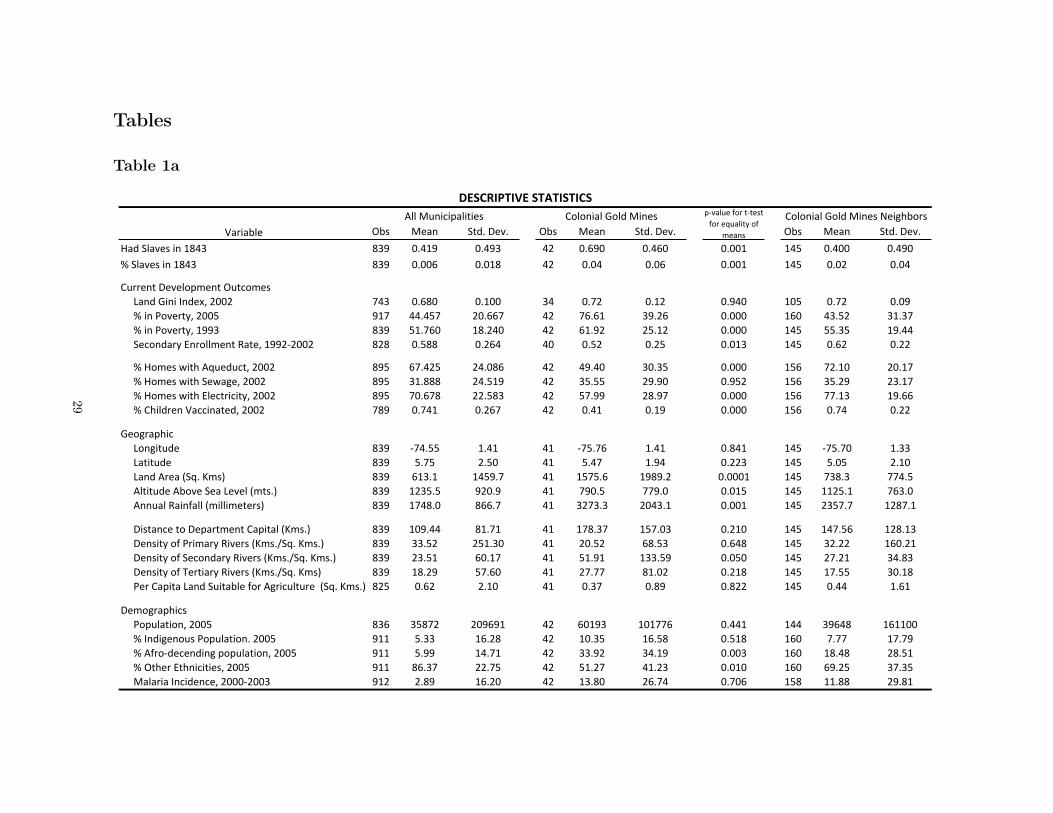
Tables

Table 1a

Variable Obs Mean Std. Dev. Obs Mean Std. Dev. Obs Mean Std. Dev.Had Slaves in 1843 839 0.419 0.493 42 0.690 0.460 0.001 145 0.400 0.490% Slaves in 1843 839 0.006 0.018 42 0.04 0.06 0.001 145 0.02 0.04

Current Development Outcomes Land Gini Index, 2002 743 0.680 0.100 34 0.72 0.12 0.940 105 0.72 0.09 % in Poverty, 2005 917 44.457 20.667 42 76.61 39.26 0.000 160 43.52 31.37 % in Poverty, 1993 839 51.760 18.240 42 61.92 25.12 0.000 145 55.35 19.44 Secondary Enrollment Rate, 1992-­‐2002 828 0.588 0.264 40 0.52 0.25 0.013 145 0.62 0.22

% Homes with Aqueduct, 2002 895 67.425 24.086 42 49.40 30.35 0.000 156 72.10 20.17 % Homes with Sewage, 2002 895 31.888 24.519 42 35.55 29.90 0.952 156 35.29 23.17 % Homes with Electricity, 2002 895 70.678 22.583 42 57.99 28.97 0.000 156 77.13 19.66 % Children Vaccinated, 2002 789 0.741 0.267 42 0.41 0.19 0.000 156 0.74 0.22

Geographic Longitude 839 -­‐74.55 1.41 41 -­‐75.76 1.41 0.841 145 -­‐75.70 1.33 Latitude 839 5.75 2.50 41 5.47 1.94 0.223 145 5.05 2.10 Land Area (Sq. Kms) 839 613.1 1459.7 41 1575.6 1989.2 0.0001 145 738.3 774.5 Altitude Above Sea Level (mts.) 839 1235.5 920.9 41 790.5 779.0 0.015 145 1125.1 763.0 Annual Rainfall (millimeters) 839 1748.0 866.7 41 3273.3 2043.1 0.001 145 2357.7 1287.1

Distance to Department Capital (Kms.) 839 109.44 81.71 41 178.37 157.03 0.210 145 147.56 128.13 Density of Primary Rivers (Kms./Sq. Kms.) 839 33.52 251.30 41 20.52 68.53 0.648 145 32.22 160.21 Density of Secondary Rivers (Kms./Sq. Kms.) 839 23.51 60.17 41 51.91 133.59 0.050 145 27.21 34.83 Density of Tertiary Rivers (Kms./Sq. Kms) 839 18.29 57.60 41 27.77 81.02 0.218 145 17.55 30.18 Per Capita Land Suitable for Agriculture (Sq. Kms.) 825 0.62 2.10 41 0.37 0.89 0.822 145 0.44 1.61

Demographics Population, 2005 836 35872 209691 42 60193 101776 0.441 144 39648 161100 % Indigenous Population. 2005 911 5.33 16.28 42 10.35 16.58 0.518 160 7.77 17.79 % Afro-­‐decending population, 2005 911 5.99 14.71 42 33.92 34.19 0.003 160 18.48 28.51 % Other Ethnicities, 2005 911 86.37 22.75 42 51.27 41.23 0.010 160 69.25 37.35 Malaria Incidence, 2000-­‐2003 912 2.89 16.20 42 13.80 26.74 0.706 158 11.88 29.81

Colonial Gold Mines p-­‐value for t-­‐test for equality of

means

Colonial Gold Mines NeighborsAll MunicipalitiesDESCRIPTIVE STATISTICS

29

Table 1b

Variable Obs Mean Std. Dev. Obs Mean Std. Dev. Obs Mean Std. Dev.Had Slaves in 1843 839 0.419 0.493 42 0.690 0.460 0.001 145 0.400 0.490% Slaves in 1843 839 0.006 0.018 42 0.04 0.06 0.001 145 0.02 0.04

Historical Development Outcomes Literacy Rate, 1918 577 0.271 0.124 33 0.28 0.13 0.491 99 0.30 0.12 School Enrollment, 1918 577 0.065 0.047 33 0.06 0.03 0.003 99 0.08 0.04 Vaccine Coverage, 1918 577 0.299 0.204 33 0.27 0.13 0.634 99 0.29 0.16

Adult Literacy Rate, 1938 640 0.463 0.164 33 0.35 0.13 0.000 118 0.453 0.13 % Buildings with Aqueduct, 1938 641 0.048 0.093 33 0.02 0.02 0.000 118 0.051 0.03 % Buildings with Electricity, 1938 641 0.071 0.111 33 0.02 0.03 0.000 118 0.060 0.03 % Buildings with Sewage, 1938 641 0.023 0.058 33 0.005 0.01 0.001 118 0.017 0.02

Contemporary State Capacity Per Capita Tax Collection, 2002 895 29919 44364 42 27035 27054 0.258 156 22400 22451 Per Capita Municipality Public Employees, 1995 837 2.116 1.848 42 1.95 1.68 0.795 144 2.03 2.00 Per 1000 Police Posts, 1995 801 0.097 0.093 40 0.06 0.07 0.342 142 0.07 0.06

Economic Structure Official Labor Share in Agriculture, 2008 907 0.054 0.097 42 0.043 0.055 0.727 158 0.048 0.076 Official Labor Share in Mining, 2008 907 0.153 0.164 42 0.190 0.221 0.028 158 0.130 0.136 Official Labor Share in Manufacturing, 2008 907 0.166 0.195 42 0.113 0.144 0.140 158 0.159 0.187 Official Labor Share in Government Services, 2008 907 0.117 0.158 42 0.078 0.080 0.117 158 0.124 0.184

Historical State Capacity Count of Number of Colonial Offices in 1794* 840 0.540 0.816 42 1.26 1.17 0.000 145 0.50 0.97 Number of Crown Employees in 1794 840 6.192 134.95 42 2.17 2.65 0.714 145 3.54 24.27* Colonial Public Offices include a State monopoly administration for Aguardiente and Gunpowder, a State monopoly administration for Tobbaco and Cards (estancos), a Postal Office, and a Tax CollectionOffice (alcabala). Thus, this variable can take values from 0 to 4.

DESCRIPTIVE STATISTICSAll Municipalities Colonial Gold Mines p-­‐value for t-­‐test

for equality of means

Colonial Gold Mines Neighbors

30

Table 2

Neighbor-­‐Pair Fixed Effects ModelsQuality 1 Quality 2 Quality 3 Quality 4 Quality 5 Quality 6 Quality 7 Quality 8

(1) (2) (3) (4) (5) (6) (7) (8)Colonial Gold Mines Dummy -­‐0.003 -­‐0.001 -­‐0.013 -­‐0.015 0.01 0.02 -­‐0.079 0.082

(0.004) (0.001) (0.017) (0.021) (0.012) (0.046) (0.066) (0.063)

Department Fixed Effects N N N N N N N NObservations 354 354 354 354 354 354 354 354R-­‐squared 0.69 0.50 0.69 0.57 0.65 0.71 0.67 0.67

Agriculture Livestock Conservation Water Valleys Mountains Hills Plains(9) (10) (11) (12) (13) (14) (15) (16)

Colonial Gold Mines Dummy -­‐0.025 -­‐0.017 0.03 0.013 -­‐0.021 -­‐0.038 0.047 0.000(0.061) (0.040) (0.056) (0.010) (0.024) (0.048) (0.045) (0.001)

Department Fixed Effects N N N N N N N NObservations 354 354 354 354 354 354 354 354R-­‐squared 0.66 0.6 0.74 0.51 0.68 0.76 0.74 0.54Standard errors are robust to arbitrary heteroskedasticity.Constant and coefficients on controls not reported.Soil qualities 1-­‐8 are classified by IGAC according to their natural aptitude for agriculture in the following way: Quality 1 soils are those with "none of very few use limitations, apt for crops and need only ordinary management practices to conserve their productivity".Quality 2 soils are those with "slight use limitations either due to their soil, topography, drainage, or climate. Require some practices to avoid erosion".Quality 3 soils are those with "moderate limitations due to soil depth, erosion, fertility, slope, drainage or climate. They require intensive conservation practices".Quality 4 soils are those with "severe limitations due to steep slopes, low soil depth, low fertility, poor drainage, frequent flooding or saltiness. Require intensive conservation practices".Quality 5 soils are those with "limitations due to flooding or rocky surfaces that limit usage to grasslands or forest".Quality 6 soils are those with "permanent unalterable limitations such as very steep slopes, high erosion susceptibility, rockiness, low soil depth, poor drainage, frequent flooding, lowhumidity retention, excessive salt or sodium. Their use is limited to grasslands or forest".Quality 7 soils are those with "severe limitations due to extreme slopes, low soil depth, rockiness, high salt and/or sodium contents poor drainage and unfavorable climate. Their useis limited to forest".Quality 8 soils are those with "extremely severe limitations due to soil, topography, drainage or climate that limit their use to conservation".Soil suitabilities and topology are also from IGAC.Source: Instituto Geográfico Agustín Codazzi IGAC (n.d.). Manual para el Uso de las Estadísticas de Zonas Físicas Homogeneas, Carreteras y Suelos.

LAND CHARACTERISTICS IN GOLD-­‐MINE AND NON-­‐GOLD-­‐MINE MUNICIPALITIES: OLS MODELSSoil Quality Shares

Soil Suitability Shares Topology Shares

31

Table 3

(1) (2) (3) (4) (5) (6) (7) (8) (9) (10) (11) (12) (13) (14) (15) (16)HadSlavesin1843 15.992 12.401 12.126 10.090 6.533 5.526 5.726 6.340 ‐0.122 ‐0.063 ‐0.100 ‐0.067 ‐0.071 ‐0.064 ‐0.065 ‐0.056

(2.454) (2.748) (2.731) (3.062) (2.940) (3.458) (2.680) (2.993) (0.043) (0.031) (0.042) (0.031) (0.035) (0.031) (0.033) (0.029)

Frac=onofSlavesin1843 69.246 38.787 25.891 15.564 ‐1.085 ‐0.616 ‐0.198 ‐0.247(29.349) (37.514) (41.892) (47.515) (0.347) (0.389) (0.431) (0.443)

σξ2 13.374 14.246 9.031 8.366 0.000 0.000 0.000 0.000

σν2 259.23 261.80 220.47 225.22 0.043 0.044 0.039 0.039R‐squared 0.482 0.487 0.639 0.639 0.443 0.443 0.560 0.560 0.257 0.272 0.378 0.392 0.200 0.204 0.327 0.330

GeographicControls N N Y Y N N Y Y N N Y Y N N Y YObserva=ons 352 352 352 352 179 179 179 179 336 336 336 336 172 172 172 172

(17) (18) (19) (20) (21) (22) (23) (24) (25) (26) (27) (28) (29) (30) (31) (32)HadSlavesin1843 ‐0.311 ‐0.229 ‐0.291 ‐0.230 ‐0.139 ‐0.108 ‐0.145 ‐0.105 0.056 0.039 0.033 0.033 0.029 0.027 0.023 0.017

(0.035) (0.036) (0.038) (0.041) (0.034) (0.033) (0.036) (0.037) (0.016) (0.018) (0.014) (0.017) (0.019) (0.021) (0.016) (0.015)

Frac=onofSlavesin1843 ‐1.561 ‐1.185 ‐0.887 ‐1.035 0.271 0.418 0.394 0.481(0.401) (0.505) (0.430) (0.522) (0.310) (0.329) (0.320) (0.251)

σξ2 0.000 0.000 0.000 0.000 0.000 0.000 0.000 0.000

σν2 0.041 0.039 0.040 0.038 0.007 0.007 0.005 0.005R‐squared 0.333 0.371 0.428 0.457 0.337 0.370 0.389 0.414 0.387 0.429 0.523 0.563 0.314 0.342 0.504 0.539

GeographicControls N N Y Y N N Y Y N N Y Y N N Y YObserva=ons 352 352 352 352 179 179 179 179 248 248 248 248 129 129 129 129StandarderrorsfortheNeighbor‐PairFixedEffectsmodelsarerobusttoarbitraryheteroskedas=city.

StandarderrorsfortheRandomEffectsmodelsarerobusttoarbitrarywithin‐neighborhoodheteroskedas=city.

Constantandcoefficientsoncontrolsnotreported.

Geographiccontrolsinclude:Shareofcul=vablelandpercapita,densityofprimaryrivers,densityofsecondaryrivers,densityofter=aryrivers,distancetothedepartmentcapital,

millimetersofannualrainfall,eleva=onabovesealevel,landarea,la=tude,andlongitude.

Allmodelsincludedepartmentfixed‐effects.

Par=alR‐squaredfortheNeighbor‐PairFixedEffectsmodels,whichexcludesthecontribu=onofthefixedeffectstothefitofthemodel

LONG‐RUNEFFECTOFSLAVERYONDEVELOPMENTOUTCOMES:OLSMODELSPovertyRate1993

Neighbor‐PairFixedEffectsModels RandomEffectsModels Neighbor‐PairFixedEffectsModels RandomEffectsModelsSecondaryEnrollmentRateAverage1992‐2002

PercentChildrenVaccinated2002 LandGini2002Neighbor‐PairFixedEffectsModels RandomEffectsModels Neighbor‐PairFixedEffectsModels RandomEffectsModels

32

Table 4

(1) (2) (3) (4) (5) (6) (7) (8) (9) (10)Colonial Gold Mines Presence 0.378 0.384 0.371 0.237 0.375 0.369 0.363 0.399 0.259 0.400

(0.048) (0.057) (0.061) (0.060) (0.061) (0.065) (0.072) (0.089) (0.083) (0.089)

Colonial State Presence Index, 1794 0.143 0.146(0.027) (0.025)

Crown Employees, 1794 0.0026 0.002(0.0014) (0.0009)

R-­‐squared 0.254 0.352 0.515 0.558 0.520 0.187 0.249 0.415 0.481 0.422Geographic Controls N Y Y Y Y N Y Y Y YQuartic on Geographic Controls N N Y Y Y N N Y Y YObservations 352 352 348 348 348 179 179 177 177 177*1st stages for the Poverty rate 1993, Poverty rate 2005, Vaccination rate 2002, Electricity coverage 2002, and Aqueduct coverage 2002 regression samples.Standard errors for the Neighbor-­‐Pair Fixed Effects models are robust to arbitrary heteroskedasticity.Standard errors for the Random Effects models are robust to arbitrary within-­‐neighborhood heteroskedasticity.Constant and coefficients on controls not reported.Geographic controls include: Share of cultivable land per capita, density of primary rivers, density of secondary rivers, density of tertiary rivers,distance to the department capital, millimeters of annual rainfall, elevation above sea level, land area, latitude, and longitude.All models include department fixed-­‐effects.Partial R-­‐squared for the Neighbor-­‐Pair Fixed Effects models, which excludes the contribution of the fixed effects to the fit of the model

FIRST STAGES OF THE IV MODELS: SLAVE PRESENCE ON COLONIAL GOLD MINES PRESENCEHad Slaves in 1843*

Random Effects ModelsNeighbor-­‐Pair Fixed Effects Models

33

Table 5

(1) (2) (3) (4) (5) (6) (7) (8)Had Slaves in 1843 12.938 11.356 14.628 13.142 -­‐0.114 -­‐0.087 -­‐0.127 -­‐0.106

(3.929) (3.935) (7.095) (6.892) (0.047) (0.052) (0.063) (0.062)

σξ2 13.374 9.031 0.000 0.000σν2 259.23 220.47 0.043 0.0391st Stage F-­‐statistic 2.190 2.217 3.181 2.345 2.318 2.430 3.069 2.462p-­‐value 0.000 0.000 0.000 0.001 0.000 0.000 0.001 0.001Geographic Controls N Y N Y N Y N YObservations 352 352 179 179 336 336 172 172

(9) (10) (11) (12) (13) (14) (15) (16)Had Slaves in 1843 -­‐0.249 -­‐0.251 -­‐0.247 -­‐0.254 0.087 0.045 0.048 0.040

(0.066) (0.074) (0.097) (0.107) (0.017) (0.015) (0.024) (0.021)

σξ2 0.000 0.000 0.000 0.000σν2 0.041 0.040 0.007 0.0051st Stage F-­‐statistic 2.190 2.217 3.181 2.345 2.312 2.200 3.233 1.963p-­‐value 0.000 0.000 0.000 0.001 0.000 0.000 0.001 0.015Geographic Controls N Y N Y N Y N YObservations 352 352 179 179 248 248 129 129Standard errors for the Neighbor-­‐Pair Fixed Effects models are robust to arbitrary heteroskedasticity.Standard errors for the Random Effects models are robust to arbitrary within-­‐neighborhood heteroskedasticity.Constant and coefficients on controls not reported.Geographic controls include: Share of cultivable land per capita, density of primary rivers, density of secondary rivers, density of tertiary rivers, distance to the department capital, millimeters of annual rainfall, elevation above sea level, land area, latitude, and longitude.All models include department fixed-­‐effects.

Percent Children Vaccinated 2002 Land Gini 2002Neighbor-­‐Pair Fixed Effects Models Random Effects Models Neighbor-­‐Pair Fixed Effects Models Random Effects Models

LONG-­‐RUN EFFECT OF SLAVERY ON DEVELOPMENT OUTCOMES: IV MODELSPoverty Rate 1993 Secondary Enrollment Rate Average 1992-­‐2002

Neighbor-­‐Pair Fixed Effects Models Random Effects Models Neighbor-­‐Pair Fixed Effects Models Random Effects Models

34

Table 6

(1) (2) (3) (4) (5) (6) (7) (8)Had Slaves in 1843 -­‐0.020 -­‐0.016 -­‐0.010 -­‐0.010 -­‐0.029 -­‐0.017 -­‐0.016 -­‐0.015

(0.008) (0.010) (0.007) (0.008) (0.034) (0.034) (0.028) (0.031)

σξ2 0.000 0.000 0.000 0.000σν2 0.001 0.001 0.023 0.020R-­‐squared 0.379 0.582 0.322 0.532 0.206 0.375 0.162 0.347Geographic Controls N Y N Y N Y N YObservations 216 216 111 111 216 216 111 111

(9) (10) (11) (12) (13) (14) (15) (16)Had Slaves in 1843 -­‐0.069 -­‐0.047 -­‐0.033 -­‐0.030 -­‐0.017 -­‐0.013 -­‐0.0074 -­‐0.0062

(0.015) (0.021) (0.019) (0.018) (0.006) (0.007) (0.0038) (0.0047)

σξ2 0.001 0.001 0.000 0.000σν2 0.011 0.007 0.001 0.001R-­‐squared 0.487 0.649 0.444 0.638 0.245 0.375 0.221 0.321Geographic Controls N Y N Y N Y N YObservations 242 242 123 123 242 242 123 123Standard errors for the Neighbor-­‐Pair Fixed Effects models are robust to arbitrary heteroskedasticity.Standard errors for the Random Effects models are robust to arbitrary within-­‐neighborhood heteroskedasticity.Constant and coefficients on controls not reported.Geographic controls include: Share of cultivable land per capita, density of primary rivers, density of secondary rivers, density of tertiary rivers, distance to the department capital, millimeters of annual rainfall, elevation above sea level, land area, latitude, and longitude.All models include department fixed-­‐effects.Partial R-­‐squared for the Neighbor-­‐Pair Fixed Effects models, which excludes the contribution of the fixed effects to the fit of the model

Literacy Rate 1938Neighbor-­‐Pair Fixed Effects Models Random Effects Models

Aqueduct Coverage 1938Neighbor-­‐Pair Fixed Effects Models Random Effects Models

LONG-­‐RUN EFFECT OF SLAVERY ON INTERMEDIATE DEVELOPMENT OUTCOMES: OLS MODELSSchool Enrollment 1918 Vaccine Coverage 1918

Neighbor-­‐Pair Fixed Effects Models Random Effects Models Neighbor-­‐Pair Fixed Effects Models Random Effects Models

35

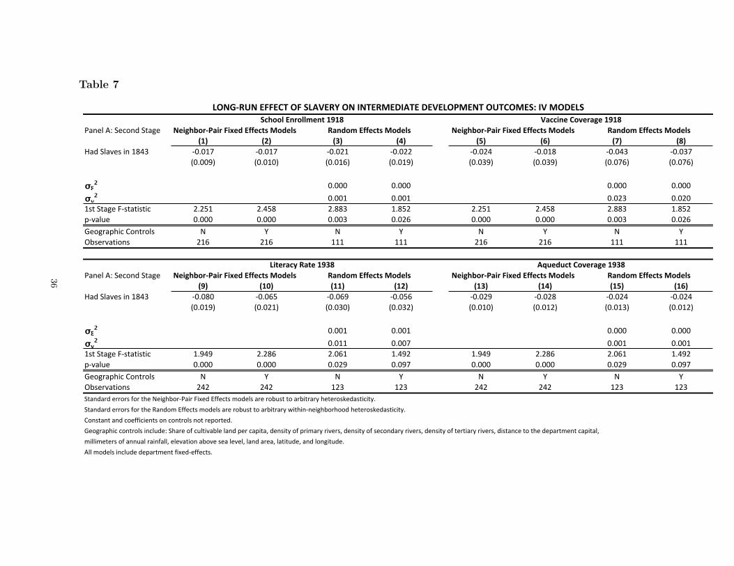
Table 7

Panel A: Second Stage(1) (2) (3) (4) (5) (6) (7) (8)

Had Slaves in 1843 -­‐0.017 -­‐0.017 -­‐0.021 -­‐0.022 -­‐0.024 -­‐0.018 -­‐0.043 -­‐0.037(0.009) (0.010) (0.016) (0.019) (0.039) (0.039) (0.076) (0.076)

σξ2 0.000 0.000 0.000 0.000σν2 0.001 0.001 0.023 0.0201st Stage F-­‐statistic 2.251 2.458 2.883 1.852 2.251 2.458 2.883 1.852p-­‐value 0.000 0.000 0.003 0.026 0.000 0.000 0.003 0.026Geographic Controls N Y N Y N Y N YObservations 216 216 111 111 216 216 111 111

Panel A: Second Stage(9) (10) (11) (12) (13) (14) (15) (16)

Had Slaves in 1843 -­‐0.080 -­‐0.065 -­‐0.069 -­‐0.056 -­‐0.029 -­‐0.028 -­‐0.024 -­‐0.024(0.019) (0.021) (0.030) (0.032) (0.010) (0.012) (0.013) (0.012)

σξ2 0.001 0.001 0.000 0.000σν2 0.011 0.007 0.001 0.0011st Stage F-­‐statistic 1.949 2.286 2.061 1.492 1.949 2.286 2.061 1.492p-­‐value 0.000 0.000 0.029 0.097 0.000 0.000 0.029 0.097Geographic Controls N Y N Y N Y N YObservations 242 242 123 123 242 242 123 123Standard errors for the Neighbor-­‐Pair Fixed Effects models are robust to arbitrary heteroskedasticity.Standard errors for the Random Effects models are robust to arbitrary within-­‐neighborhood heteroskedasticity.Constant and coefficients on controls not reported.Geographic controls include: Share of cultivable land per capita, density of primary rivers, density of secondary rivers, density of tertiary rivers, distance to the department capital, millimeters of annual rainfall, elevation above sea level, land area, latitude, and longitude.All models include department fixed-­‐effects.

Literacy Rate 1938Neighbor-­‐Pair Fixed Effects Models Random Effects Models

Aqueduct Coverage 1938Neighbor-­‐Pair Fixed Effects Models Random Effects Models

LONG-­‐RUN EFFECT OF SLAVERY ON INTERMEDIATE DEVELOPMENT OUTCOMES: IV MODELSSchool Enrollment 1918 Vaccine Coverage 1918

Neighbor-­‐Pair Fixed Effects Models Random Effects Models Neighbor-­‐Pair Fixed Effects Models Random Effects Models

36

Table 8

Had Slaves in 1843 1.000Colonial State Presence Index, 1794 0.406 1.000Crown Employees, 1794 0.098 0.327 1.000Obs: 177

SLAVERY AND COLONIAL STATE PRESENCE: CORRELATIONS

37

Table 9

(1) (2) (3) (4) (5) (6) (7) (8) (9) (10) (11) (12)Had Slaves in 1843 13.972 15.484 14.362 5.786 6.938 6.148 -­‐0.116 -­‐0.141 -­‐0.122 -­‐0.057 -­‐0.078 -­‐0.065

(3.497) (3.608) (3.517) (3.431) (3.407) (3.378) (0.046) (0.055) (0.046) (0.044) (0.048) (0.045)

Colonial State Presence Index, 1794 -­‐1.029 -­‐1.199 0.019 0.022(1.401) (1.406) (0.020) (0.019)

Crown Employees, 1794 -­‐0.099 -­‐0.069 0.002 0.001(0.040) (0.030) (0.001) (0.0003)

σξ2 0.000 0.000 0.000 0.000 0.000 0.000σν2 195.71 195.81 194.63 0.04 0.04 0.04R-­‐squared 0.742 0.742 0.744 0.676 0.678 0.680 0.504 0.505 0.515 0.431 0.437 0.446Quartic on Geographic Controls Y Y Y Y Y Y Y Y Y Y Y YObservations 348 348 348 177 177 177 332 332 332 170 170 170

(13) (14) (15) (16) (17) (18) (19) (20) (21) (22) (23) (24)Had Slaves in 1843 -­‐0.308 -­‐0.280 -­‐0.312 -­‐0.169 -­‐0.153 -­‐0.169 0.020 0.020 0.020 0.011 0.007 0.011

(0.045) (0.058) (0.046) (0.044) (0.046) (0.045) (0.015) (0.019) (0.015) (0.019) (0.020) (0.019)

Colonial State Presence Index, 1794 -­‐0.019 -­‐0.016 0.000 0.005(0.023) (0.024) (0.008) (0.007)

Crown Employees, 1794 0.001 0.000 -­‐0.0001 0.0001(0.0006) (0.0003) (0.0002) (0.0002)

σξ2 0.000 0.000 0.000 0.000 0.000 0.000σν2 0.039 0.04 0.04 0.005 0.005 0.005R-­‐squared 0.528 0.541 0.529 0.469 0.472 0.469 0.685 0.687 0.685 0.662 0.663 0.662Quartic on Geographic Controls Y Y Y Y Y Y Y Y Y Y Y YObservations 348 348 348 177 177 177 244 244 244 127 127 127Standard errors for the Neighbor-­‐Pair Fixed Effects models are robust to arbitrary heteroskedasticity.Standard errors for the Random Effects models are robust to arbitrary within-­‐neighborhood heteroskedasticity.Constant and coefficients on controls not reported.Geographic controls include: Share of cultivable land per capita, density of primary rivers, density of secondary rivers, density of tertiary rivers, distance to the department capital, millimeters of annual rainfall, elevation above sea level, land area, latitude, and longitude.All models include department fixed-­‐effects.Partial R-­‐squared for the Neighbor-­‐Pair Fixed Effects models, which excludes the contribution of the fixed effects to the fit of the model

Percent Children Vaccinated 2002 Land Gini 2002Neighbor-­‐Pair Fixed Effects Models Random Effects Models Neighbor-­‐Pair Fixed Effects Models Random Effects Models

LONG-­‐RUN EFFECT OF SLAVERY ON DEVELOPMENT OUTCOMES: OLS MODELS WITH ADDITIONAL CONTROLSPoverty Rate 1993 Secondary Enrollment Rate Average 1992-­‐2002

Neighbor-­‐Pair Fixed Effects Models Random Effects Models Neighbor-­‐Pair Fixed Effects Models Random Effects Models

38

Table 10

Panel A: Second Stage(1) (2) (3) (4) (5) (6) (7) (8) (9) (10) (11) (12)

Had Slaves in 1843 12.752 22.330 12.551 11.885 20.774 11.872 -­‐0.089 -­‐0.146 -­‐0.084 -­‐0.091 -­‐0.167 -­‐0.090(4.872) (8.118) (3.753) (6.736) (10.553) (5.371) (0.053) (0.056) (0.051) (0.058) (0.071) (0.058)

Colonial State Presence Index, 1794 -­‐3.782 -­‐3.758 0.024 0.034(1.863) (2.238) (0.012) (0.016)

Crown Employees, 1794 -­‐0.043 -­‐0.039 0.001 0.001(0.037) (0.024) (0.0004) (0.0002)

σξ2 0.000 0.000 0.000 0.000 0.000 0.000σν2 195.71 195.81 194.63 0.038 0.038 0.0371st Stage F-­‐statistic 2.651 3.257 2.674 2.408 3.046 2.408 2.807 3.262 2.810 2.349 2.939 2.350p-­‐value 0.000 0.000 0.000 0.000 0.000 0.000 0.000 0.000 0.000 0.000 0.000 0.000Quartic on Geographic Controls Y Y Y Y Y Y Y Y Y Y Y YObservations 348 348 348 177 177 177 332 332 332 170 170 170

Panel A: Second Stage(13) (14) (15) (16) (17) (18) (19) (20) (21) (22) (23) (24)

Had Slaves in 1843 -­‐0.259 -­‐0.414 -­‐0.256 -­‐0.231 -­‐0.360 -­‐0.231 0.073 0.128 0.073 0.037 0.040 0.037(0.081) (0.123) (0.052) (0.106) (0.147) (0.070) (0.021) (0.041) (0.021) (0.022) (0.031) (0.022)

Colonial State Presence Index, 1794 0.061 0.054 -­‐0.020 -­‐0.001(0.025) (0.029) (0.008) (0.006)

Crown Employees, 1794 0.001 0.0004 -­‐0.0001 0.0000(0.0005) (0.0003) (0.0001) (0.0001)

σξ2 0.000 0.000 0.000 0.000 0.000 0.000σν2 0.039 0.0389 0.0392 0.005 0.0046 0.00461st Stage F-­‐statistic 2.651 3.257 2.674 2.408 3.046 2.408 2.416 2.842 2.389 1.594 1.922 1.577p-­‐value 0.000 0.000 0.000 0.000 0.000 0.000 0.000 0.000 0.000 0.038 0.006 0.041Quartic on Geographic Controls Y Y Y Y Y Y Y Y Y Y Y YObservations 348 348 348 177 177 177 244 244 244 127 127 127Standard errors for the Neighbor-­‐Pair Fixed Effects models are robust to arbitrary heteroskedasticity.Standard errors for the Random Effects models are robust to arbitrary within-­‐neighborhood heteroskedasticity.Constant and coefficients on controls not reported.Geographic controls include: Share of cultivable land per capita, density of primary rivers, density of secondary rivers, density of tertiary rivers, distance to the department capital, millimeters of annual rainfall, elevation above sea level, land area, latitude, and longitude.All models include department fixed-­‐effects.

Percent Children Vaccinated 2002 Land Gini 2002Neighbor-­‐Pair Fixed Effects Models Random Effects Models Neighbor-­‐Pair Fixed Effects Models Random Effects Models

LONG-­‐RUN EFFECT OF SLAVERY ON DEVELOPMENT OUTCOMES: IV MODELS WITH ADDITIONAL CONTROLSPoverty Rate 1993 Secondary Enrollment Rate Average 1992-­‐2002

Neighbor-­‐Pair Fixed Effects Models Random Effects Models Neighbor-­‐Pair Fixed Effects Models Random Effects Models

39

Figures

Figure 1

BOG

SANT

METACUND

ANT

GUAJ

VALLE

TOLIMAHUILAATLANTCALDAS CESARBOYBOLRISARCORD

NRT SANT

MAGD

SUCRENARINO

CAUCA

CHOCO

500

1000

1500

2000

2500

Per C

apita

GDP

in 2

001

(thou

sand

s of

Pes

os)

0 2 4 6 8 10Proportion of Slaves in 1843

DepartmentsProportion of Slaves in 1843 vs. Per Capita GDP in 2001

020

4060

8010

0Po

verty

Rat

e in

199

3

0 .05 .1 .15 .2 .25Proportion of Slaves in 1843

Municipalities (sample of neighborhoods)Proportion of Slaves in 1843 vs. Poverty Rate in 1993

40

Figure 2

Source: West (1952).

41

Figure 3

Very Light Green = 0-0.052, Light Green = 0.052-0.104, Green = 0.104-0.156, Green Blue = 0.156-0.208, Blue= 0.208-0.26

42

Figure 4

43

Figure 5

0.2

.4.6

.8Fr

actio

n

0 .05 .1 .15 .2 .25Proportion of Slaves in 1843

Sample of Neighbors1843 Slavery Intensity Distribution

44

Appendix 1: Random Effects Correlation Structure

As a simple illustration, if the sample had 2 gold-mine municipalities g1 and g2, a, b, c share a borderwith g1 and a, c, d, e share a border with g2, then M(a) = M(c) = g1, g2, M(b) = g1, andM(d) = M(e) = g2. In this case, the Random Effects covariance matrix would take the form:

Ω =

g1 a b c g2 d e

g1 σ2ξ + σ2

ν σ2ξ σ2

ξ σ2ξ 0 0 0

a σ2ξ 2σ2

ξ + σ2ν σ2

ξ 2σ2ξ σ2

ξ σ2ξ σ2

ξ

b σ2ξ σ2

ξ σ2ξ + σ2

ν σ2ξ 0 0 0

c σ2ξ 2σ2

ξ σ2ξ 2σ2

ξ + σ2ν σ2

ξ σ2ξ σ2

ξ

g2 0 σ2ξ 0 σ2

ξ σ2ξ + σ2

ν σ2ξ σ2

ξ

d 0 σ2ξ 0 σ2

ξ σ2ξ σ2

ξ + σ2ν σ2

ξ

e 0 σ2ξ 0 σ2

ξ σ2ξ σ2

ξ σ2ξ + σ2

ν

The feasible random effects estimator requires prior estimation of Ω. Given the covariance structureof the unobservables, σ2

ξ and σ2ν can be estimated as follows:

σ2ξ =

|N |+ |M ||N |+ |M | −K

( ∑i∈N

∑j∈N,j 6=i uiuj∑

i∈N∑j∈N,j 6=i |M(i) ∩M(j)|

+

∑i∈N

∑g∈M(i) uiug∑

i∈N M(i)

)(10)

where K is the number of covariates. The term |N |+|M ||N |+|M |−K is a degrees-of-freedom adjustment.

Now define a to be the sum of the diagonal of Ω. Thus,

a ≡ (|N |+ |M |)σ2ν +

(|M |+

∑i∈N|M(i)|

)σ2ξ (11)

By defining a to be the empirical analogous of a,

a =∑s

u2s (12)

We can use the definition of a to solve for σ2ν :

σ2ν =

a−(|M |+

∑i∈N |M(i)|

)σ2ξ

|N |+ |M |(13)

Replacing (10) and (12) in (13), we obtain an estimate of σ2ν :

σ2ν =

|N |+ |M ||N |+ |M | −K

a−(|M |+

∑i∈N |M(i)|

) (σ2ξ|N |+|M |−k|N |+|M |

)|N |+ |M |

(14)

Thus, the estimated variance matrix Ω uses equations (10) and (14) in Ω.

45

Appendix 2

Table A2.1

Neighbor-­‐Pair Fixed Effects Random Effects Neighbor-­‐Pair Fixed Effects Random Effects Neighbor-­‐Pair Fixed Effects Random Effects(1) (2) (3) (4) (5) (6)

Had Slaves in 1843 5.117 2.753 -­‐12.698 -­‐3.713 -­‐12.746 -­‐6.925(2.549) (3.306) (3.292) (2.476) (3.413) (2.549)

σξ2 31.823 0.000 0.000σν2 318.51 240.47 268.98R-­‐squared 0.640 0.543 0.641 0.599 0.617 0.560Geographic Controls Y Y Y Y Y YObservations 352 179 352 179 352 179

Neighbor-­‐Pair Fixed Effects Random Effects Neighbor-­‐Pair Fixed Effects Random Effects Neighbor-­‐Pair Fixed Effects Random Effects(7) (8) (9) (10) (11) (12)

Had Slaves in 1843 0.005 -­‐0.025 0.001 0.000 -­‐0.012 -­‐0.008(0.025) (0.022) (0.005) (0.003) (0.008) (0.0057)

σξ2 0.001 0.000 0.000σν2 0.008 0.0004 0.001R-­‐squared 0.582 0.532 0.250 0.194 0.341 0.308Geographic Controls Y Y Y Y Y YObservations 216 111 242 123 242 123Standard errors for the Neighbor-­‐Pair Fixed Effects models are robust to arbitrary heteroskedasticity.Standard errors for the Random Effects models are robust to arbitrary within-­‐neighborhood heteroskedasticity.Constant and coefficients on controls not reported.Geographic controls include: Share of cultivable land per capita, density of primary rivers, density of secondary rivers, density of tertiary rivers, distance to the department capital, millimeters of annual rainfall, elevation above sea level, land area, latitude, and longitude.All models include department fixed-­‐effects.Partial R-­‐squared for the Neighbor-­‐Pair Fixed Effects models, which excludes the contribution of the fixed effects to the fit of the model

Literacy Rate 1918 Sewage Coverage 1938

Aquedcut Coverage 2002

Electricity Coverage 1938

LONG-­‐RUN EFFECT OF SLAVERY ON ADDITIONAL DEVELOPMENT OUTCOMES: OLS MODELSPoverty Rate 2005 Electricity Coverage 2002

46

Table A2.2

(1) (2) (3) (4) (5) (6) (7) (8)Colonial Gold Mines Presence 0.378 0.384 0.369 0.363 0.339 0.350 0.360 0.374

(0.048) (0.057) (0.065) (0.072) (0.048) (0.058) (0.065) (0.075)

R-­‐squared 0.254 0.352 0.187 0.249 0.249 0.359 0.188 0.267Geographic Controls N Y N Y N Y N YObservations 352 352 179 179 336 336 172 172

(9) (10) (11) (12) (13) (14) (15) (16)Colonial Gold Mines Presence 0.329 0.339 0.321 0.272 0.309 0.300 0.350 0.357

(0.058) (0.065) (0.084) (0.083) (0.056) (0.064) (0.079) (0.081)

R-­‐squared 0.299 0.383 0.224 0.292 0.260 0.351 0.170 0.237Geographic Controls N Y N Y N Y N YObservations 216 216 111 111 242 242 123 123

(17) (18) (19) (20)Colonial Gold Mines Presence 0.369 0.370 0.380 0.384

(0.054) (0.064) (0.070) (0.082)

R-­‐squared 0.304 0.376 0.215 0.267Geographic Controls N Y N YObservations 248 248 129 129*1st stages for the Poverty rate 1993, Poverty rate 2005, Vaccination rate 2002, Electricity coverage 2002, and Aqueduct coverage 2002 regression samples.**1st stage for the Secondary Enrollment rate 1992-­‐2002 regressions sample.***1st stage for the 1918 regressions sample.****1st stage for the 1938 regressions sample.*****1st stage for the Land Gini 2002 regressions sample.Standard errors for the Neighbor-­‐Pair Fixed Effects models are robust to arbitrary heteroskedasticity.Standard errors for the Random Effects models are robust to arbitrary within-­‐neighborhood heteroskedasticity.Constant and coefficients on controls not reported.Geographic controls include: Share of cultivable land per capita, density of primary rivers, density of secondary rivers, density of tertiary rivers,distance to the department capital, millimeters of annual rainfall, elevation above sea level, land area, latitude, and longitude.All models include department fixed-­‐effects.Partial R-­‐squared for the Neighbor-­‐Pair Fixed Effects models, which excludes the contribution of the fixed effects to the fit of the model

FIRST STAGES OF THE IV MODELS: SLAVE PRESENCE ON COLONIAL GOLD MINES PRESENCEHad Slaves in 1843* Had Slaves in 1843**

Neighbor-­‐Pair Fixed Effects Models Random Effects Models Neighbor-­‐Pair Fixed Effects Models Random Effects Models

Had Slaves in 1843*****Neighbor-­‐Pair Fixed Effects Models Random Effects Models

Had Slaves in 1843*** Had Slaves in 1843****Neighbor-­‐Pair Fixed Effects Models Random Effects Models Neighbor-­‐Pair Fixed Effects Models Random Effects Models

47

Table A2.3

Panel A: Second Stage Neighbor-­‐Pair Fixed Effects Random Effects Neighbor-­‐Pair Fixed Effects Random Effects Neighbor-­‐Pair Fixed Effects Random Effects(1) (2) (3) (4) (5) (6)

Had Slaves in 1843 5.388 7.307 -­‐7.541 -­‐7.179 -­‐9.792 -­‐11.036(3.301) (5.848) (3.510) (5.736) (3.714) (6.108)

σξ2 31.823 0.000 0.000σν2 318.51 240.47 268.981st Stage F-­‐statistic 2.217 2.345 2.217 2.345 2.217 2.345p-­‐value 0.000 0.001 0.000 0.001 0.000 0.001Geographic Controls Y Y Y Y Y YObservations 352 179 352 179 352 179

Panel A: Second Stage Neighbor-­‐Pair Fixed Effects Random Effects Neighbor-­‐Pair Fixed Effects Random Effects Neighbor-­‐Pair Fixed Effects Random Effects(7) (8) (9) (10) (11) (12)

Had Slaves in 1843 0.031 0.010 -­‐0.009 -­‐0.009 -­‐0.022 -­‐0.020(0.026) (0.050) (0.007) (0.008) (0.010) (0.012)

σξ2 0.001 0.000 0.000σν2 0.008 0.0004 0.0011st Stage F-­‐statistic 2.458 1.852 2.286 1.492 2.286 1.492p-­‐value 0.000 0.026 0.000 0.097 0.000 0.097Geographic Controls Y Y Y Y Y YObservations 216 111 242 123 242 123Standard errors for the Neighbor-­‐Pair Fixed Effects models are robust to arbitrary heteroskedasticity.Standard errors for the Random Effects models are robust to arbitrary within-­‐neighborhood heteroskedasticity.Constant and coefficients on controls not reported.Geographic controls include: Share of cultivable land per capita, density of primary rivers, density of secondary rivers, density of tertiary rivers, distance to the department capital, millimeters of annual rainfall, elevation above sea level, land area, latitude, and longitude.All models include department fixed-­‐effects.

LONG-­‐RUN EFFECT OF SLAVERY ON ADDITIONAL DEVELOPMENT OUTCOMES: IV MODELSPoverty Rate 2005 Electricity Coverage 2002 Aquedcut Coverage 2002

Electricity Coverage 1938Literacy Rate 1918 Sewage Coverage 1938

48

Table A2.4

Neighbor-­‐Pair Fixed Effects Models

(1) (2) (3) (4) (5) (6) (7) (8)Colonial Gold Mines Dummy -­‐0.006 -­‐0.017 0.065 0.056 -­‐0.017 0.003 -­‐0.049 -­‐0.029

(0.015) (0.012) (0.049) (0.054) (0.032) (0.049) (0.021) (0.023)

Department Fixed Effects N Y N Y N Y N YQuartic on Geographic Controls N Y N Y N Y N YObservations 364 358 364 358 364 358 364 358R-­‐squared 0.53 0.73 0.56 0.73 0.69 0.84 0.6 0.77Standard errors are robust to arbitrary heteroskedasticity.Constant and coefficients on controls not reported.Geographic controls include: Share of cultivable land per capita, density of primary rivers, density of secondary rivers, density of tertiary rivers,distance to the department capital, millimeters of annual rainfall, elevation above sea level, land area, latitude, and longitude.The quartic polynomials include distance to the department capital, millimeters of annual rainfall, elevation above sea level, land area, latitude, and longitude.

SECTORAL COMPOSITION OF EMPLOYMENT IN GOLD-­‐MINE AND NON-­‐GOLD-­‐MINE MUNICIPALITIES: OLS MODELSEmployment Share 2008

Agriculture Mining Manufacturing Government

49

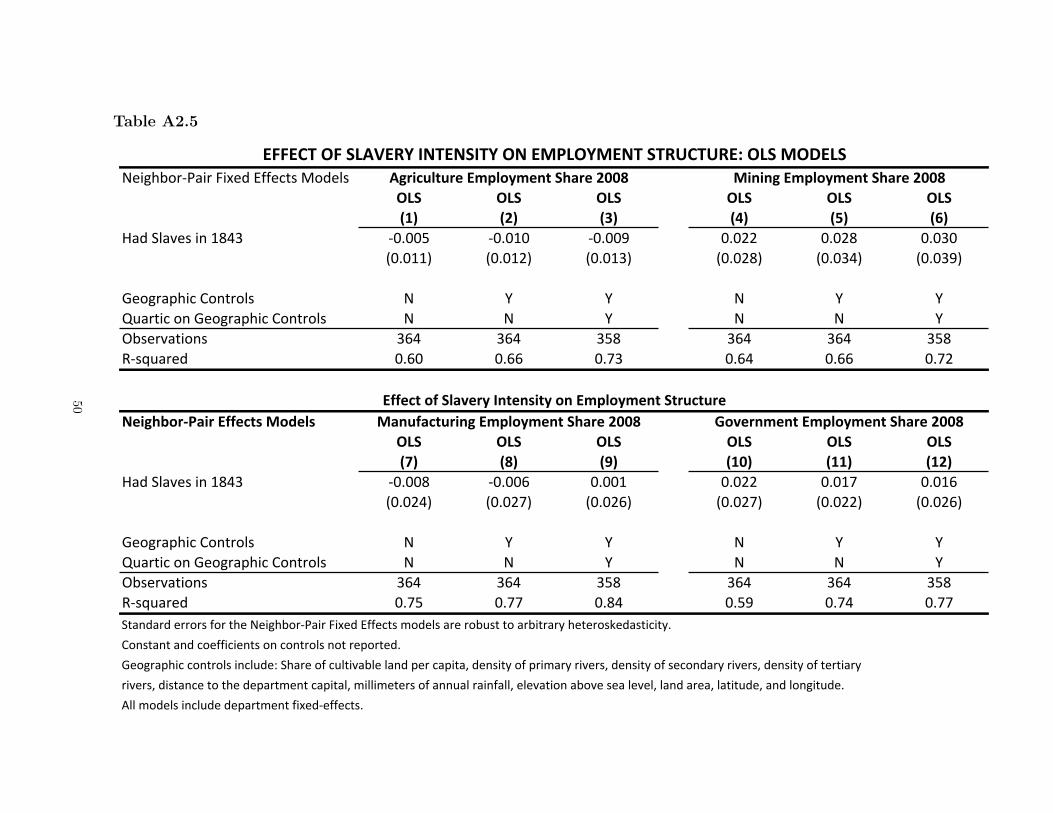
Table A2.5

Neighbor-­‐Pair Fixed Effects ModelsOLS OLS OLS OLS OLS OLS(1) (2) (3) (4) (5) (6)

Had Slaves in 1843 -­‐0.005 -­‐0.010 -­‐0.009 0.022 0.028 0.030(0.011) (0.012) (0.013) (0.028) (0.034) (0.039)

Geographic Controls N Y Y N Y YQuartic on Geographic Controls N N Y N N YObservations 364 364 358 364 364 358R-­‐squared 0.60 0.66 0.73 0.64 0.66 0.72

Neighbor-­‐Pair Effects ModelsOLS OLS OLS OLS OLS OLS(7) (8) (9) (10) (11) (12)

Had Slaves in 1843 -­‐0.008 -­‐0.006 0.001 0.022 0.017 0.016(0.024) (0.027) (0.026) (0.027) (0.022) (0.026)

Geographic Controls N Y Y N Y YQuartic on Geographic Controls N N Y N N YObservations 364 364 358 364 364 358R-­‐squared 0.75 0.77 0.84 0.59 0.74 0.77Standard errors for the Neighbor-­‐Pair Fixed Effects models are robust to arbitrary heteroskedasticity.Constant and coefficients on controls not reported.Geographic controls include: Share of cultivable land per capita, density of primary rivers, density of secondary rivers, density of tertiary rivers, distance to the department capital, millimeters of annual rainfall, elevation above sea level, land area, latitude, and longitude.All models include department fixed-­‐effects.

EFFECT OF SLAVERY INTENSITY ON EMPLOYMENT STRUCTURE: OLS MODELSAgriculture Employment Share 2008 Mining Employment Share 2008

Effect of Slavery Intensity on Employment StructureManufacturing Employment Share 2008 Government Employment Share 2008

50

Table A2.6

Neighbor-­‐Pair Fixed Effects ModelsOLS OLS OLS OLS OLS OLS OLS OLS OLS(1) (2) (3) (4) (5) (6) (7) (8) (9)

Had Slaves in 1843 17,164.8 16,825.9 8,602.9 -­‐0.135 -­‐0.288 -­‐0.076 -­‐0.036 -­‐0.027 -­‐0.024(5,117.3) (4,957.3) (5,521.7) (0.340) (0.337) (0.319) (0.009) (0.010) (0.013)

Geographic Controls N Y Y N Y Y N Y YQuartic on Geographic Controls N N Y N N Y N N YObservations 352 352 352 348 348 348 340 340 340R-­‐squared 0.65 0.74 0.80 0.67 0.72 0.77 0.74 0.76 0.81Standard errors for the Neighbor-­‐Pair Fixed Effects models are robust to arbitrary heteroskedasticity.Constant and coefficients on controls not reported.Geographic controls include: Share of cultivable land per capita, density of primary rivers, density of secondary rivers, density of tertiary rivers, distance to the department capital, millimeters of annual rainfall, elevation above sea level, land area, latitude, and longitude.All models include department fixed-­‐effects.

EFFECT OF SLAVERY INTENSITY ON STATE CAPACITY OUTCOMES: OLS MODELS Per Capita Tax Collection 2002 Per Capita Municipality Employees 1995 Per 1000 Police Posts 1995

51