Finding Distractors In Images

Ohad FriedPrinceton University

ohad@cs.princeton.edu

Eli ShechtmanAdobe Researchelishe@adobe.com

Dan B GoldmanAdobe Research

dgoldman@adobe.com

Adam FinkelsteinPrinceton Universityaf@cs.princeton.edu

Abstract

We propose a new computer vision task we call “distrac-tor prediction.” Distractors are the regions of an image thatdraw attention away from the main subjects and reduce theoverall image quality. Removing distractors — for example,using in-painting — can improve the composition of an im-age. In this work we created two datasets of images withuser annotations to identify the characteristics of distrac-tors. We use these datasets to train an algorithm to predictdistractor maps. Finally, we use our predictor to automati-cally enhance images.

1. IntroductionTaking pictures is easy, but editing them is not. Profes-

sional photographers expend great care and effort to com-pose aesthetically-pleasing, high-impact imagery. Imageediting software like Adobe Photoshop empowers photog-raphers to achieve this impact by manipulating pictures withtremendous control and flexibility – allowing them to care-fully post-process good photos and turn them into greatphotos. However, for most casual photographers this effortis neither possible nor warranted. Last year Facebook re-ported that people were uploading photos at an average rateof 4,000 images per second. The overwhelming majority ofthese pictures are casual – they effectively chronicle a mo-ment, but without much work on the part of the photogra-pher. Such cases may benefit from semi- or fully-automaticenhancement methods.

Features like “Enhance” in Apple’s iPhoto or “AutoTone” in Photoshop supply one-click image enhancement,but they mainly manipulate global properties such as ex-posure and tone. Likewise, Instagram allows novices toquickly and easily apply eye-catching filters to their images.Although they have some more localized effects like edgedarkening, they apply the same recipe to any image. How-ever, local, image-specific enhancements like removing dis-tracting areas are not handled well by automatic methods.There are many examples of such distractors – trash onthe ground, the backs of tourists visiting a monument, a

car driven partially out of frame, etc. Removing distrac-tors demands a time-consuming editing session in whichthe user manually selects the target area and then appliesfeatures like iPhoto’s “Retouch Tool” or Photoshop’s “Con-tent Aware Fill” to swap that area with pixels copied fromelsewhere in the image.

In this work we take the first steps towards semi-automatic distractor removal from images. The main chal-lenge towards achieving this goal is to automatically iden-tify what types of image regions a person might want toremove, and to detect such regions in arbitrary images. Toaddress this challenge we conduct several studies in whichpeople mark distracting regions in a large collection of im-ages, and then we use this dataset to train a model based onimage features.

Our main contributions are: (1) defining a new taskcalled “distractor prediction”, (2) collecting a large-scaledatabase with annotations of distractors, (3) training a pre-diction model that can produce distractor maps for arbitraryimages, and (4) using our prediction model to automaticallyremove distractors from images.

In the following sections we describe related work (Sec-tion 2), describe and analyze our datasets (Section 3), ex-plain our distractor prediction model (Section 4), evaluateour predictor (Section 5) and present applications of dis-tractor prediction (Section 6). With this publication we alsomake available an annotated dataset containing images withdistractors as well as code for both analyzing the dataset andcomputing distractor maps.

2. Related WorkA primary characteristic of distractors is that they attract

our visual attention, so they are likely to be somewhatcorrelated with models of visual saliency. Computationalsaliency methods can be roughly divided into two groups:human fixation detection [13, 11, 15] and salient objectdetection [7, 6, 22, 20]. Most of these methods used ground-truth gaze data collected in the first 3-5 seconds of viewing(a few get up to 10 seconds) [15]. Although we found somecorrelation between distractor locations and these early-viewing gaze fixations, it was not high. Our hypothesis

1

Figure 1. User annotations. Top: 35 user annotations for oneinput image. Bottom, from left to right: input image, averageannotation, overlay of thresholded annotation with input image.We collected 11244 such annotations for 1073 images.

is that humans start looking at distractors after longerperiods of time, and perhaps only look directly at themwhen following different viewing instructions. Existingcomputational saliency methods are thus insufficient todefine visual distractors, because the main subject in a photowhere people look first usually has a high saliency value.Moreover, many of these methods (especially in the secondcategory) include components that attenuate the saliencyresponse away from the center of the image or from thehighest peaks - exactly in the places we found distractorsto be most prevalent.

Another line of related work focuses on automatic im-age cropping [29, 21, 34]. While cropping can often removesome visual distractors, it might also remove important con-tent. For instance, many methods just try to crop around themost salient object. Advanced cropping methods [34] alsoattempt to optimize the layout of the image, which mightnot be desired by the user and is not directly related to de-tecting distractors. Removing distractors is also related tothe visual aesthetics literature [16, 19, 23, 30] as distrac-tors can clutter the composition of an image, or disrupt itslines of symmetry. In particular, aesthetics principles likesimplicity [16] are related to our task. However, the com-putational methods involved in measuring these propertiesdon’t directly detect distractors and don’t propose ways toremove them.

Image and video enhancement methods have been pro-posed to detect dirt spots, sparkles [17], line scratches [14]and rain drops [8]. In addition, a plethora of popularcommercial tools have been developed for face retouching:These typically offer manual tools for removing or attenu-ating blemishes, birth marks, wrinkles etc. There have beenalso a few attempts to automate this process (e.g., [32])

Mechanical Turk Mobile App

Number of images 403 376Annotations per image 27.8 on average 1User initiated No YesImage source Previous datasets App users

Table 1. Dataset comparison.

that require face-specific techniques. Another interestingwork [28] focused on detecting and de-emphasizing dis-tracting texture regions that might be more salient than themain object. All of the above methods are limited to a cer-tain type of distractor or image content, but in this work weare interested in a more general-purpose solution.

3. Datasets

We created two datasets with complementary properties.The first consists of user annotations gathered via AmazonMechanical Turk. The second includes real-world use casesgathered via a dedicated mobile app. The Mechanical Turkdataset is freely available, including all annotations, butthe second dataset is unavailable to the public due to theapp’s privacy policy. We use it for cross-database validationof our results (Section 5). Table 1 and the followingsubsections describe the two datasets.

3.1. Mechanical Turk Dataset (MTurk)

For this dataset we combined several previous datasetsfrom the saliency literature [1, 15, 18] for a total of 1073images. We created a Mechanical Turk task in which userswere shown 10 of these images at random and instructed asfollows:

For each image consider what regions of the image aredisturbing or distracting from the main subject. Pleasemark the areas you might point out to a professionalphoto editor to remove or tone-down to improve the im-age. Some images might not have anything distractingso it is ok to skip them.

The users were given basic draw and erase tools forimage annotation (Figure 2). We collected initial data forthe entire dataset (average of 7 annotations per image) andused it to select images containing distractors by consensus:An image passed the consensus test if more than half ofthe distractor annotations agree at one or more pixels inthe image. 403 images passed this test and were usedin a second experiment. We collected a total of 11244annotations, averaging 27.8 annotations per image in theconsensus set (figure 1).

Figure 2. Data collection interfaces. Left: MTurk interface withbasic tools for marking and removal. Right: Mobile app usinginpainting with a variable brush size, zoom level and undo/redos.

3.2. Mobile App Dataset (MApp)

Although the Mechanical Turk dataset is easy to col-lect, one might argue that it is biased: Because Mechan-ical Turk workers do not have any particular expectationsabout image enhancement and cannot see the outcome ofthe intended distractor removal, their annotations may beinconsistent with those of real users who wish to removedistractors from images. In order to address this, we alsocreated a second dataset with such images: We created afree mobile app (Figure 2) that enables users to mark andremove unwanted areas in images. The app uses a patch-based hole filling method [4] to produce a new image withthe marked area removed. The user can choose to discardthe changes, save or share them. Users can opt-in to sharetheir images for limited research purposes, and over 25% ofusers chose to do so.

Using this app, we collected over 5,000 images and over44,000 fill actions (user strokes that mark areas to removefrom the image). We then picked only images that wereexported, shared or saved by the users to their camera roll(i.e. not discarded), under the assumption that users onlysave or share images with which they are satisfied.

Users had a variety of reasons for using the app. Manyusers removed attribution or other text to repurpose imagesfrom others found on the internet. Others were simplyexperimenting with the app (e.g. removing large body partsto comical effect), or clearing large regions of an imagefor the purpose of image composites and collages. Wemanually coded the dataset to select only those images withdistracting objects removed. Despite their popularity, wealso excluded face and skin retouching examples, as theserequire special tools and our work focused on more generalimages. After this coding, we used the 376 images withdistractors as our dataset for learning.

3.3. Data Analysis

Our datasets afford an opportunity to learn what arethe common locations for distractors. Figure 3 showsthe average of all collected annotations. It is clear thatdistractors tend to appear near the boundaries of the image,

Figure 3. An average of all collected annotations. Distractors tendto appear near the image boundary.

with some bias towards the left and right edges. We use thisobservation later in Section 4.2.

We can also investigate which visual elements are themost common distractors. We created a taxonomy for thefollowing objects that appeared repeatedly as distractors inboth datasets: spot (dust or dirt on the lens or scene), high-light (saturated pixels from light sources or reflections),face, head (back or side), person (body parts other thanhead or face), wire (power or telephone), pole (telephoneor fence), line (straight lines other than wires or poles), can(soda or beer), car, crane, sign, text (portion, not a com-plete sign), camera, drawing, reflection (e.g. in imagestaken through windows), trash (garbage, typically on theground), trashcan, hole (e.g. in the ground or a wall).

Treating each annotated pixel as a score of 1, we thresh-olded the average annotation value of each image in theMTurk dataset at the top 5% value, which corresponds to0.18, and segmented the results using connected compo-nents (Figure 1). For each connected component we manu-ally coded one or more tags from the list above. The tag ob-ject was used for all objects which are not one of the othercategories, whereas unknown was used to indicate regionsthat do not correspond to discrete semantic objects. We alsoincluded three optional modifiers for each tag: boundary (aregion touching the image frame), partial (usually an oc-cluded object) and blurry. Figure 4 shows the histogramsof distractor types and modifiers. Notice that several dis-tractor types are quite common. This insight leads to a po-tential strategy for image distractor removal: training task-specific detectors for the top distractor categories. In thiswork we chose several features based on the findings of fig-ure 4 (e.g. a text detector, a car detector, a person detector,an object proposal method). An interesting direction for fu-ture work would be to implement other detectors, such aselectric wires and poles.

All distractor annotations for the MTurk dataset arefreely available for future research as part of our dataset.

4. Distractor Prediction

Given input images and user annotations, we can con-struct a model for learning distractor maps. We first seg-ment each image (section 4.1). Next we calculate features

0 50 100 150 200 250 300

camera

can

trashcan

tree

drawing

face

head

crane

hole

line

shadow

trash

sign

text

pole

reflection

car

wire

unknown

spot

highlight

person

object

Distractor Types

Number of distractors0 200 400 600 800

blurry

partial

boundary

others

Property Types

Number of distractors

Figure 4. Distractor Types. Left: histogram of distractor typesdescribed in Section 3.3. Right: histogram of distractor properties,indicating whether the distractor is close to the image boundary,occluded/cropped or blurry.

for each segment (section 4.2). Lastly, we use LASSO [31]to train a mapping from segment features to a distractorscore — the average number of distractor annotations perpixel (section 4.3). The various stages of our algorithm areshown in figure 5.

4.1. Segmentation

Per-pixel features can capture the properties of a singlepixel or some neighborhood around it, but they usually donot capture region characteristics for large regions. Thus,we first segment the image and later use that segmentationto aggregate measurements across regions. For the segmen-tation we use multi-scale combinatorial grouping (MCG)[2]. The output of MCG is in the range of [0, 1] and weuse a threshold value of 0.4 to create a hard segmentation.This threshold maximizes the mean distractor score per seg-ment over the entire dataset. We found empirically that themaximum of this objective segments distracting objects ac-curately in many images.

4.2. Features

Our datasets and annotations give us clues about theproperties of distractors and how to detect them. Thedistractors are, by definition, salient, but not all salientregions are distractors. Thus, previous features used forsaliency prediction are good candidate features for ourpredictor (but not sufficient). We also detect features thatdistinguish main subjects from salient distractors that mightbe less important, such as objects near the image boundary.Also, we found several types of common objects appeared

Figure 5. Various stages of our algorithm. Top left: original image.Top right: MCG segmentation. 2nd row: examples of 6 of our192 features. 3rd row left: our prediction, red (top three), yellow(high score) to green (low score). 3rd row right: ground truth.Bottom row: distractor removal results, with threshold values 1, 2,3, 20 from left to right. The 3 distractors are gradually removed(3 left images), but when the threshold is too high, artifacts startappearing (far right).

frequently, and included specific detectors for these objects.We calculate per-pixel and per-region features. The 60

per-pixel features are:• (3) Red, green and blue channels.

• (3) Red, green and blue probabilities (as in [15]).

• (5) Color triplet probabilities, for five median filter windowsizes (as in [15]).

• (13) Steerable pyramids [27].

• (5) Detectors: cars [10], people [10], faces [33], text [24],horizon [25, 15].

• (2) Distance to the image center and to the closest imageboundary.

• (7)∗ Saliency prediction methods [12, 13, 20, 22, 25].

• (2)∗ Object proposals [35]: all objects, top 20 objects. Wesum the scores to create a single map.

• (2) Object proposals [35]: all objects contained in the outer25% of the image. We create 2 maps: one by summing allscores and another by picking the maximal value per pixel.

• (9) All features marked with ∗, attenuated by F = 1 −G/max (G). G is a Gaussian the size of the image with a

standard deviation of 0.7∗√d1 ∗ d2 (d1 and d2 are the height

and width of the image) and centered at the image center.

• (9) All features marked with ∗, attenuated by F as definedabove, but with the Gaussian centered at the pixel with themaximal feature value.

All the per-pixel features are normalized to have zeromean and unit variance.

To use these per-pixel features as per-segment features,we aggregate them in various ways: For each image seg-ment, we calculate the mean, median and max for each ofthe 60 pixel features, resulting in 180 pixel-based featuresper segment.

Lastly, we add a few segment-specific features: area,major and minor axis lengths, eccentricity, orientation,convex area, filled area, Euler number, equivalent diameter,solidity, extent and perimeter (all as defined by the Matlabfunction regionprops). All features are concatenated,creating a vector with 192 values per image segment.

4.3. Learning

For each image in our dataset we now have a segmen-tation and a feature vector per segment. We also have usermarkings. Given all the markings for a specific image, wecalculate the average marking (over all users and all seg-ment pixels) for each segment. The calculated mean is theground truth distractor score for the segment.

We use Least Absolute Selection and Shrinkage Opera-tor (LASSO) [31] to learn a mapping between segment fea-tures and a segment’s distractor score. All results in thispaper are using LASSO with 3-fold cross validation. UsingLASSO allows us to learn the importance of various fea-tures and perform feature selection (section 4.4).

Besides LASSO, we also tried linear and kernel SVM [9]and random forests with bootstrap aggregating [5]. KernelSVM and random forests failed to produce good results,possibly due to overfitting on our relatively small dataset.Linear SVM produced results almost as good as LASSO,but we chose LASSO for its ability to rank features andremove unnecessary features. Nonetheless, linear SVM ismuch faster and may be a viable alternative when trainingtime is critical.

4.4. Feature Ranking

Table 2 shows the highest scoring features for each of thedatasets. We collect the feature weights from all leave-one-out experiments using LASSO. Next we calculate the meanof the absolute value of weights, providing a measure forfeature importance. The table shows the features with thelargest mean value.

Using our feature ranking we can select a subset ofthe features, allowing a trade-off between computation andaccuracy. Using the label Fk to denote the set of k highestscoring features when trained using all features, Table 4

MTurk MApp

Torralba saliency1† Torralba saliency2†

RGB Green3 Coxel saliency3

Torralba saliency2† RGB Probability (W=0)1

Itti saliency1† RGB Probability (W=2)3

RGB Blue probability3 Text detector1

RGB Probability (W=4)1 RGB Green probability1

RGB Probability (W=2)1 Boundary object proposals1

Object proposals3‡ Hou saliency3‡

RGB Probability (W=16)1 Hou saliency1†

Distance to boundary3 Steerable Pyramids21mean 2median 3max

†attenuated with an inverted Gaussian around image center‡attenuated with an inverted Gaussian around maximal value

Table 2. Feature selection. For each dataset we list the featureswith the highest mean feature weight across all experiments.

shows results with only F5 and F10 features. Althoughthese results are less accurate than the full model, they canbe calculated much faster. (But note that feature sets Fk asdefined above are not necessarily the optimal set to use fortraining with k features.)

5. Evaluation

For evaluation, we plot a receiver operating characteris-tic (ROC) curve (true positive rate vs. false positive rate)and calculate the area under the curve (AUC) of the plot.We use a leave-one-out scheme, where all images but oneare used for training and the one is used for testing. We re-peat the leave-one-out experiment for each of our images,calculating the mean of all AUC values to produce a score.

Table 3 summarizes our results. A random baselineachieves a score of 0.5. We achieve an average AUC of 0.81for the MTurk dataset and 0.84 for the MApp dataset. TheLASSO algorithm allows us to learn which of the featuresare important (section 4.4) and we also report results usingsubsets of our features (Table 4). As expected, these resultsare not as good as the full model, but they are still usefulwhen dealing with space or time constraints (less featuresdirectly translate to less memory and less computationtime). We also report results for previous saliency methodsas well as a simple adaptation to these methods where wemultiply the saliency maps by an inverted Gaussian (asdescribed in Sec. 4.2). This comparison is rather unfairsince saliency methods try to predict all salient regionsand not just distractors. However, the low scores for thesemethods show that indeed distractor prediction requires anew model based on new features.

Method MTurk AUC MApp AUC

Random 0.50 0.50Saliency IV‡ [25] 0.55 0.56Saliency I [20] 0.57 0.53Saliency I‡ [20] 0.58 0.59Saliency II [22] 0.59 0.57Saliency II‡ [22] 0.59 0.57Saliency III‡ [12] 0.62 0.59Saliency III [12] 0.65 0.69Saliency I† [20] 0.67 0.65Saliency II† [22] 0.68 0.68Saliency III† [12] 0.70 0.75Saliency IV† [25] 0.72 0.72Saliency IV [25] 0.74 0.76Our method 0.81 0.84Average Human 0.89 -

†attenuated with an inverted Gaussian around image center‡attenuated with an inverted Gaussian around maximal value

Table 3. AUC scores. We compare against saliency predictionmethods as published, and the same methods attenuated withan inverted Gaussian, as described in Section 4.2. Our methodoutperforms all others. As an upper bound we report averagehuman score, which takes the average annotation as a predictor(per image, using a leave-one-out scheme). We also comparedagainst individual features from Table 2 (not shown): all scoreswere lower than our method with a mean score of 0.59.

Method Average # MTurk AUCof used features

Ours (F-5 features) 3.40 0.72Ours (F-10 features) 7.43 0.80Ours (all features) 28.06 0.81

Table 4. AUC scores. Results using all 192 features and subsetsF5 and F10 described in Section 4.4. Column 2 is the mean (overall experiments) of the number of features that were not zeroed outby the LASSO optimization. F10 produces a score similar to thefull model, while using 5% of the features.

5.1. Inter-Dataset Validation

Using Mechanical Turk has the advantage of allowingus to get a lot of data quickly, but might be biased awayfrom real-world scenarios. We wanted to make sure thatour images and annotation procedure indeed match distrac-tor removal “in the wild”. For that purpose we also cre-ated dataset collected using our mobile app (MApp dataset),which contains real world examples of images with distrac-tors that were actually removed by users. We performedinter-dataset tests: training on one dataset and testing on theother, the results are summarized in table 5. We show good

Train Test # of features # of used AUCDataset Dataset features

MTurk MApp 192 37 0.86MApp MTurk 192 25 0.78

Table 5. Inter-dataset AUC scores. We train on one dataset and teston the other, in order to validate that our MTurk dataset is similarenough to the real-world use cases in MApp to use for learning.

results for training on MTurk and testing on MApp (0.86)and vice versa (0.78). The MApp dataset contains a singleannotation per image (vs. 27.8 on average for the MTurkone). We therefore believe that the value 0.78 can be im-proved as the MApp dataset grows.

6. ApplicationsWe propose a few different applications of distractor

prediction. The most obvious application is automatic in-painting (Section 6.1), but the ability to identify distractingregions of an image can also be applied to down-weight theimportance of regions for image retargeting (Section 6.2).We also posit that image aesthetics and automatic croppingcan benefit from our method (Section 7).

6.1. Distractor Removal

The goal of distractor removal is to attenuate the distract-ing qualities of an image, to improve compositional clarityand focus on the main subject. For example, distracting re-gions can simply be inpainted with surrounding contents.To illustrate this application we created a simple interfacewith a single slider that allows the user to select a distractorthreshold (figure 6). All segments are sorted according totheir score and the selected threshold determines the num-ber of segments being inpainted (figure 5). For a full demoof this system please see our supplementary video. Somebefore and after examples are shown in figure 7. We chosea rank order-based user interface as it is hard to find onethreshold that would work well on all images, however wefound that if distractors exist in an image they will corre-

Figure 6. User interface for distractor removal. The user selects theamount of distracting segments they wish to remove. We refer thereader to the accompanying video for a more lively demonstration.

Figure 7. Examples of distractor removal results. Each quadruplet shows (from left to right): (1) Original image. (2) Normalized averageground-truth annotation. (3) Order of segments as predicted by our algorithm. (4) Distractor removal result. We urge the reader to zoomin or to look at the full resolution images available as supplementary material. The number of segments to remove was manually selectedfor each image. Segments are shown on a green-to-yellow scale, green being a lower score. Segment selected for removal are shown on anorange-to-red scale, red being a higher score. Notice how the red segments correlate with the ground-truth annotation. Also notice that wemanage to detect a variety of distracting elements (a sign, a person, an abstract distractor in the corner, etc.)

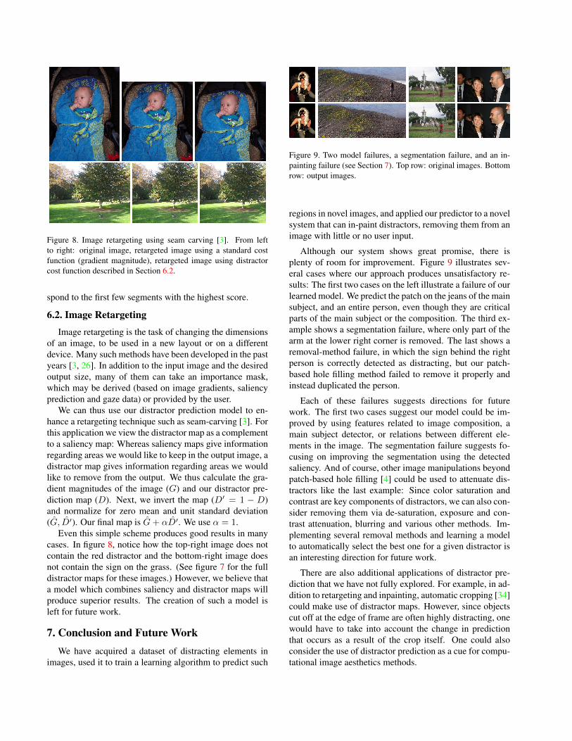
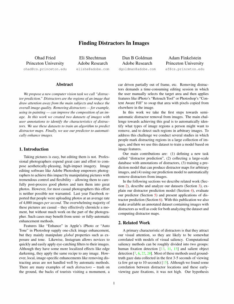
Figure 8. Image retargeting using seam carving [3]. From leftto right: original image, retargeted image using a standard costfunction (gradient magnitude), retargeted image using distractorcost function described in Section 6.2.

spond to the first few segments with the highest score.

6.2. Image Retargeting

Image retargeting is the task of changing the dimensionsof an image, to be used in a new layout or on a differentdevice. Many such methods have been developed in the pastyears [3, 26]. In addition to the input image and the desiredoutput size, many of them can take an importance mask,which may be derived (based on image gradients, saliencyprediction and gaze data) or provided by the user.

We can thus use our distractor prediction model to en-hance a retargeting technique such as seam-carving [3]. Forthis application we view the distractor map as a complementto a saliency map: Whereas saliency maps give informationregarding areas we would like to keep in the output image, adistractor map gives information regarding areas we wouldlike to remove from the output. We thus calculate the gra-dient magnitudes of the image (G) and our distractor pre-diction map (D). Next, we invert the map (D′ = 1 − D)and normalize for zero mean and unit standard deviation(G, D′). Our final map is G+ αD′. We use α = 1.

Even this simple scheme produces good results in manycases. In figure 8, notice how the top-right image does notcontain the red distractor and the bottom-right image doesnot contain the sign on the grass. (See figure 7 for the fulldistractor maps for these images.) However, we believe thata model which combines saliency and distractor maps willproduce superior results. The creation of such a model isleft for future work.

7. Conclusion and Future WorkWe have acquired a dataset of distracting elements in

images, used it to train a learning algorithm to predict such

Figure 9. Two model failures, a segmentation failure, and an in-painting failure (see Section 7). Top row: original images. Bottomrow: output images.

regions in novel images, and applied our predictor to a novelsystem that can in-paint distractors, removing them from animage with little or no user input.

Although our system shows great promise, there isplenty of room for improvement. Figure 9 illustrates sev-eral cases where our approach produces unsatisfactory re-sults: The first two cases on the left illustrate a failure of ourlearned model. We predict the patch on the jeans of the mainsubject, and an entire person, even though they are criticalparts of the main subject or the composition. The third ex-ample shows a segmentation failure, where only part of thearm at the lower right corner is removed. The last shows aremoval-method failure, in which the sign behind the rightperson is correctly detected as distracting, but our patch-based hole filling method failed to remove it properly andinstead duplicated the person.

Each of these failures suggests directions for futurework. The first two cases suggest our model could be im-proved by using features related to image composition, amain subject detector, or relations between different ele-ments in the image. The segmentation failure suggests fo-cusing on improving the segmentation using the detectedsaliency. And of course, other image manipulations beyondpatch-based hole filling [4] could be used to attenuate dis-tractors like the last example: Since color saturation andcontrast are key components of distractors, we can also con-sider removing them via de-saturation, exposure and con-trast attenuation, blurring and various other methods. Im-plementing several removal methods and learning a modelto automatically select the best one for a given distractor isan interesting direction for future work.

There are also additional applications of distractor pre-diction that we have not fully explored. For example, in ad-dition to retargeting and inpainting, automatic cropping [34]could make use of distractor maps. However, since objectscut off at the edge of frame are often highly distracting, onewould have to take into account the change in predictionthat occurs as a result of the crop itself. One could alsoconsider the use of distractor prediction as a cue for compu-tational image aesthetics methods.

References[1] H. Alers, H. Liu, J. Redi, and I. Heynderickx. Studying the

effect of optimizing the image quality in saliency regions atthe expense of background content. In Proc. SPIE, volume7529, 2010. 2

[2] P. Arbelaez, J. Pont-Tuset, J. Barron, F. Marques, and J. Ma-lik. Multiscale combinatorial grouping. In IEEE Conf. onComputer Vision and Pattern Recognition (CVPR), 2014. 4

[3] S. Avidan and A. Shamir. Seam carving for content-awareimage resizing. In ACM Trans. on Graphics (Proc. SIG-GRAPH), New York, NY, USA, 2007. ACM. 8

[4] C. Barnes, E. Shechtman, A. Finkelstein, and D. B. Gold-man. PatchMatch: A randomized correspondence algorithmfor structural image editing. ACM Trans. on Graphics (Proc.SIGGRAPH), (3), Aug. 3, 8

[5] L. Breiman. Bagging predictors. Machine Learning,24(2):123–140, 1996. 5

[6] K.-Y. Chang, T.-L. Liu, H.-T. Chen, and S.-H. Lai. Fusinggeneric objectness and visual saliency for salient object de-tection. In International Conf. on Computer Vision (ICCV),2011. 1

[7] M.-M. Cheng, G.-X. Zhang, N. Mitra, X. Huang, and S.-M.Hu. Global contrast based salient region detection. In IEEEConf. on Computer Vision and Pattern Recognition (CVPR),pages 409–416, June 2011. 1

[8] D. Eigen, D. Krishnan, and R. Fergus. Restoring an imagetaken through a window covered with dirt or rain. InInternational Conf. on Computer Vision (ICCV), pages 633–640, 2013. 2

[9] R.-E. Fan, P.-H. Chen, and C.-J. Lin. Working set selectionusing second order information for training support vectormachines. Journal of Machine Learning Research, 6:1889–1918, Dec. 2005. 5

[10] P. F. Felzenszwalb, R. B. Girshick, D. McAllester, and D. Ra-manan. Object Detection with Discriminatively Trained PartBased Models. IEEE Trans. on Pattern Analysis and Ma-chine Intelligence (PAMI), 32(9):1627–1645, 2010. 4

[11] J. Harel, C. Koch, and P. Perona. Graph-based visualsaliency. In Advances in Neural Information ProcessingSystems, pages 545–552. MIT Press, 2007. 1

[12] X. Hou and L. Zhang. Saliency Detection: A SpectralResidual Approach. In IEEE Conf. on Computer Vision andPattern Recognition (CVPR), June 2007. 4, 6

[13] L. Itti and C. Koch. A Saliency-Based Search Mechanism forOvert and Covert Shifts of Visual Attention. Vision Research,40:1489–1506, 2000. 1, 4

[14] L. Joyeux, O. Buisson, B. Besserer, and S. Boukir. Detectionand removal of line scratches in motion picture films. InIEEE Conf. on Computer Vision and Pattern Recognition(CVPR), pages 548–553, 1999. 2

[15] T. Judd, K. Ehinger, F. Durand, and A. Torralba. Learningto predict where humans look. In International Conf. onComputer Vision (ICCV), 2009. 1, 2, 4

[16] Y. Ke, X. Tang, and F. Jing. The design of high-level featuresfor photo quality assessment. In IEEE Conf. on ComputerVision and Pattern Recognition (CVPR), volume 1, pages419–426, 2006. 2

[17] A. C. Kokaram. On missing data treatment for degradedvideo and film archives: A survey and a new bayesianapproach. IEEE Trans. on Image Processing, 13(3):397–415,Mar. 2004. 2

[18] H. Liu and I. Heynderickx. Studying the added value ofvisual attention in objective image quality metrics based oneye movement data. In IEEE International Conf. on ImageProcessing (ICIP), Nov. 2009. 2

[19] W. Luo, X. Wang, and X. Tang. Content-based photo qualityassessment. In International Conf. on Computer Vision(ICCV), Nov 2011. 2

[20] R. Mairon and O. Ben-Shahar. A closer look at context:From coxels to the contextual emergence of object saliency.In European Conf. on Computer Vision (ECCV). 2014. 1, 4,6

[21] L. Marchesotti, C. Cifarelli, and G. Csurka. A frameworkfor visual saliency detection with applications to imagethumbnailing. In International Conf. on Computer Vision(ICCV), pages 2232–2239, 2009. 2

[22] R. Margolin, A. Tal, and L. Zelnik-Manor. What Makes aPatch Distinct? IEEE Conf. on Computer Vision and PatternRecognition (CVPR), pages 1139–1146, June 2013. 1, 4, 6

[23] N. Murray, L. Marchesotti, and F. Perronnin. Ava: A large-scale database for aesthetic visual analysis. In IEEE Conf.on Computer Vision and Pattern Recognition (CVPR), 2012.(In press). 2

[24] L. Neumann and J. Matas. Real-time scene text localizationand recognition. IEEE Conf. on Computer Vision and PatternRecognition (CVPR), 2012. 4

[25] A. Oliva and A. Torralba. Modeling the shape of the scene: Aholistic representation of the spatial envelope. Internationaljournal of computer vision, 42(3):145–175, 2001. 4, 6

[26] M. Rubinstein, D. Gutierrez, O. Sorkine, and A. Shamir. Acomparative study of image retargeting. ACM Transactionson Graphics, 29(6):160:1–160:10, Dec. 2010. 8

[27] E. Simoncelli and W. Freeman. The Steerable Pyramid: AFlexible Architecture For Multi-Scale Derivative Computa-tion. IEEE International Conf. on Image Processing (ICIP),1995. 4

[28] S. L. Su, F. Durand, and M. Agrawala. De-emphasis ofdistracting image regions using texture power maps. InApplied Perception in Graphics & Visualization, pages 164–164, New York, NY, USA, 2005. ACM. 2

[29] B. Suh, H. Ling, B. B. Bederson, and D. W. Jacobs. Au-tomatic thumbnail cropping and its effectiveness. In Pro-ceedings of the 16th Annual ACM Symposium on User In-terface Software and Technology, UIST ’03, pages 95–104,New York, NY, USA, 2003. ACM. 2

[30] X. Tang, W. Luo, and X. Wang. Content-Based PhotoQuality Assessment. IEEE Transactions on Multimedia(TMM), 2013. 2

[31] R. Tibshirani. Regression Shrinkage and Selection Via theLasso. Journal of the Royal Statistical Society, Series B,58:267–288, 1994. 4, 5

[32] W.-S. Tong, C.-K. Tang, M. S. Brown, and Y.-Q. Xu.Example-based cosmetic transfer. Computer Graphics andApplications, Pacific Conference on, 0:211–218, 2007. 2

[33] P. Viola and M. Jones. Robust Real-time Object Detection.In International Journal of Computer Vision (IJCV), 2001. 4

[34] J. Yan, S. Lin, S. Bing Kang, and X. Tang. Learningthe change for automatic image cropping. In IEEE Conf.on Computer Vision and Pattern Recognition (CVPR), June2013. 2, 8

[35] C. L. Zitnick and P. Dollar. Edge Boxes: Locating ObjectProposals from Edges. In European Conf. on ComputerVision (ECCV), 2014. 4