HAL Id: lirmm-01964467https://hal-lirmm.ccsd.cnrs.fr/lirmm-01964467

Submitted on 8 Jan 2019

HAL is a multi-disciplinary open accessarchive for the deposit and dissemination of sci-entific research documents, whether they are pub-lished or not. The documents may come fromteaching and research institutions in France orabroad, or from public or private research centers.

L’archive ouverte pluridisciplinaire HAL, estdestinée au dépôt et à la diffusion de documentsscientifiques de niveau recherche, publiés ou non,émanant des établissements d’enseignement et derecherche français ou étrangers, des laboratoirespublics ou privés.

Finding a most parsimonious or likely tree in a networkwith respect to an alignment

Steven Kelk, Fabio Pardi, Celine Scornavacca, Leo van Iersel

To cite this version:Steven Kelk, Fabio Pardi, Celine Scornavacca, Leo van Iersel. Finding a most parsimonious or likelytree in a network with respect to an alignment. Journal of Mathematical Biology, Springer Verlag(Germany), 2019, 78 (1-2), pp.527-547. �10.1007/s00285-018-1282-2�. �lirmm-01964467�

Journal of Mathematical Biologyhttps://doi.org/10.1007/s00285-018-1282-2 Mathematical Biology

Finding a most parsimonious or likely tree in a networkwith respect to an alignment

Steven Kelk1 · Fabio Pardi2 · Celine Scornavacca3 · Leo van Iersel4

Received: 13 July 2017 / Revised: 16 May 2018© The Author(s) 2018

AbstractPhylogenetic networks are often constructed bymergingmultiple conflicting phyloge-netic signals into a directed acyclic graph. It is interesting to explore whether a networkconstructed in this way induces biologically-relevant phylogenetic signals that werenot present in the input. Here we show that, given a multiple alignment A for a setof taxa X and a rooted phylogenetic network N whose leaves are labelled by X , it isNP-hard to locate a most parsimonious phylogenetic tree displayed by N (with respectto A) even when the level of N—the maximum number of reticulation nodes within abiconnected component—is 1 and A contains only 2 distinct states. (If, additionally,gaps are allowed the problem becomes APX-hard.) We also show that under the sameconditions, and assuming a simple binary symmetric model of character evolution,finding a most likely tree displayed by the network is NP-hard. These negative resultscontrast with earlier work on parsimony in which it is shown that if A consists ofa single column the problem is fixed parameter tractable in the level. We concludewith a discussion of why, despite the NP-hardness, both the parsimony and likelihoodproblem can likely be well-solved in practice.

Keywords Phylogenetic tree · Phylogenetic network · Maximum parsimony ·Maximum likelihood · NP-hardness · APX-hardness

Mathematics Subject Classification 92D15 · 68Q25 · 92D20

1 Introduction

Rooted phylogenetic networks are generalizations of rooted phylogenetic trees thatallow horizontal evolutionary events such as horizontal gene transfer, recombinationand hybridization to be modelled (Huson et al. 2010; Morrison 2011; Gusfield 2014).This is achieved by allowing nodes with indegree 2 or higher, known as reticulation

Kelk and Pardi have contributed equally to this article.

Extended author information available on the last page of the article

123

S. Kelk et al.

nodes. Recent years have seen an explosion of interest in constructing rooted phyloge-netic networks, fuelled by the growing awareness that incongruence in phylogeneticand phylogenomic datasets is not simply a question of evolutionary “noise”, butsometimes the result of evolutionary phenomena more complex than speciation andmutation (e.g. Zhaxybayeva and Doolittle 2011; Abbott et al. 2013; Vuilleumier andBonhoeffer 2015).

Although many modelling questions surrounding the construction of phylogeneticnetworks are still to be answered, it is commonplace to associate a rooted phylogeneticnetwork with the set of rooted phylogenetic trees that it contains (“displays”). Infor-mally speaking, a rooted phylogenetic network displays a rooted phylogenetic tree ifthe tree can be topologically embedded inside the network. A network is not neces-sarily defined by the set of trees it displays, but the notion of display is neverthelessa recurring theme in the literature, since networks themselves are often constructedby merging phylogenetic trees subject to some optimality criterion. It is well-knownthat it is NP-hard to determine whether a network displays a given tree (Kanj et al.2008), although on many restricted classes of phylogenetic networks the problem ispolynomial-time solvable (Van Iersel et al. 2010; Fakcharoenphol et al. 2015; Gam-bette et al. 2015).

Although it is important to be able to determine whether a network displays a giventree, we may also wish to ask what the “best” tree is within the network, subject tosome optimality criterion. For example, given a network N and a multiple alignmentA, we may wish to ask for a tree T displayed by N with lowest parsimony score withrespect to A. Similarly, if the network is decorated by edge lengths or probabilities,we may wish to identify a most likely tree displayed by the network, that is, a treethat maximizes the probability of generating A, under a given model of evolution.Such questions are natural, as the two following examples show. First, phylogeneticnetworks are often constructed by topologically merging incongruent phylogeneticsignals (e.g. Kelk and Scornavacca 2014), and it is insightful to ask whether thenetwork thus constructed displays trees which have interesting properties (such as alow parsimony score or a high likelihood) which were not in the input. Second, wemay wish to perform classical phylogenetic tree construction under criteria such asmaximum parsimony or maximum likelihood (e.g. Jin et al. 2006, 2007), but withinthe restricted space of trees displayed by a given network.

Problems of the above kind are already known to be NP-hard, since it is NP-hard to determine a most parsimonious tree T displayed by a given network N evenwhen the alignment A consists of a single column and the network is binary (Fischeret al. 2015). However, the gadgets used in that hardness reduction produce networkswith very high level, where level is the maximum number of reticulation nodes in abiconnected component of the network. On the positive side, the same article showsthat the problem on an alignment consisting of a single column is FPT in the level ofthe network. This means that, on a network with level k, the problem can be solved intime f (k) · poly(n) where f is a function that depends only on k and n is the size ofthe network. Such results are useful in practice, when (as is often the case) k is small.

The question emergeswhether the positive FPT result goes throughwhen A does notconsist of a single column, but potentially many columns – a problem introduced morethan one decade ago (Nakhleh et al. 2005). Here we show that this is not the case. We

123

Finding a most parsimonious or likely tree in a network. . .

prove the rather negative result that locating amost parsimonious tree in a rooted binarynetwork N is NP-hard, even under the following restricted circumstances: (1) eachbiconnected component of the network contains exactly one reticulation node (i.e. is“level-1”); (2) each biconnected component of the network has exactly three outgoingarcs; (3) the alignment A consists of two states. If indel symbols are permitted then theproblem is not only NP-hard, but also difficult to approximate well (APX-hard). If anyof the conditions (1)-(3) are further strengthened (respectively: the network becomes atree; the reticulation nodes become redundant; the alignment becomes uninformative),the problembecomes trivially solvable, so in some sense this is a “best possible” (or the“worst possible”, depending on your perspective) hardness result. Next, we considerthe question of identifying a most likely tree in the network. We obtain NP-hardnessunder the same restrictions (1)-(3), subject to the simple binary symmetric model ofcharacter evolution. It is no coincidence that restrictions (1)-(3) again apply, since thehardness of the likelihood question is established by reducing the parsimony variant ofthe problem to it. Specifically, we show that a most likely tree displayed by a networkwith sufficiently short branches is necessarily also a most parsimonious tree.

Although the main results in this paper are negative, some reasons for hope aregiven in the conclusion.

2 Preliminaries

A rooted binary phylogenetic network N on a set X of taxa is a directed acyclic graphwhere the leaves (nodes of indegree-1 and outdegree-0) are bijectively labelled by X ,there is a unique root (a node of indegree-0 and outdegree-2) and all other nodes areeither tree nodes (indegree-1 and outdegree-2) or reticulation nodes (indegree-2 andoutdegree-1). For brevity we henceforth simply use the term network. A rooted binaryphylogenetic tree (henceforth tree) is a phylogenetic network without any reticulationnodes.A cherry is a pair of taxa that share a commonparent.A rooted binary caterpillaris a tree with exactly one cherry.

The level of a network N is the maximum number of reticulation nodes in a bicon-nected component of the undirected graph underpinning N . In this articlewewill focusexclusively on level-1 networks. In level-1 networks, maximal biconnected compo-nents that are not single edges are simple cycles that contain exactly one reticulationnode; such biconnected components are called galls. An arc whose tail (but not head)is a node of a gall is called an outgoing arc.

A character f is a surjective mapping f : X → S where S is a set of discretestates. When S contains two states we say that f is a binary character. Given a treeT = (V , E) and a character f , both on X , we say that f : V → S is an extensionof f to T if f (x) = f (x) for all x ∈ X . The number of mutations induced by f (onT ), denoted l f (T ), is the number of edges {u, v} ∈ E such that f (u) �= f (v). Theparsimony score of f with respect to T , denoted l f (T ), is the minimum number ofmutations induced ranging over all extensions f of f . Any extension that achievesthis minimum is called an optimal extension. An optimal extension can be computedin polynomial time using Fitch’s algorithm (Fitch 1971), which for completeness

123

S. Kelk et al.

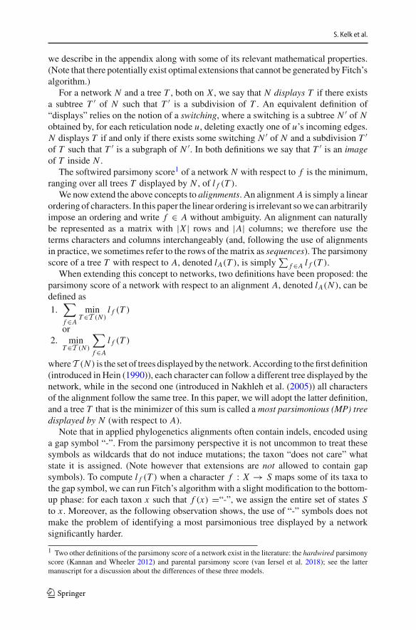
we describe in the appendix along with some of its relevant mathematical properties.(Note that there potentially exist optimal extensions that cannot be generated by Fitch’salgorithm.)

For a network N and a tree T , both on X , we say that N displays T if there existsa subtree T ′ of N such that T ′ is a subdivision of T . An equivalent definition of“displays” relies on the notion of a switching, where a switching is a subtree N ′ of Nobtained by, for each reticulation node u, deleting exactly one of u’s incoming edges.N displays T if and only if there exists some switching N ′ of N and a subdivision T ′of T such that T ′ is a subgraph of N ′. In both definitions we say that T ′ is an imageof T inside N .

The softwired parsimony score1 of a network N with respect to f is the minimum,ranging over all trees T displayed by N , of l f (T ).

We now extend the above concepts to alignments. An alignment A is simply a linearordering of characters. In this paper the linear ordering is irrelevant sowe can arbitrarilyimpose an ordering and write f ∈ A without ambiguity. An alignment can naturallybe represented as a matrix with |X | rows and |A| columns; we therefore use theterms characters and columns interchangeably (and, following the use of alignmentsin practice, we sometimes refer to the rows of thematrix as sequences). The parsimonyscore of a tree T with respect to A, denoted lA(T ), is simply

∑f ∈A l f (T ).

When extending this concept to networks, two definitions have been proposed: theparsimony score of a network with respect to an alignment A, denoted lA(N ), can bedefined as

1.∑

f ∈A

minT ∈T (N )

l f (T )

or2. min

T ∈T (N )

∑

f ∈A

l f (T )

whereT (N ) is the set of trees displayedby thenetwork.According to thefirst definition(introduced in Hein (1990)), each character can follow a different tree displayed by thenetwork, while in the second one (introduced in Nakhleh et al. (2005)) all charactersof the alignment follow the same tree. In this paper, we will adopt the latter definition,and a tree T that is the minimizer of this sum is called a most parsimonious (MP) treedisplayed by N (with respect to A).

Note that in applied phylogenetics alignments often contain indels, encoded usinga gap symbol “-”. From the parsimony perspective it is not uncommon to treat thesesymbols as wildcards that do not induce mutations; the taxon “does not care” whatstate it is assigned. (Note however that extensions are not allowed to contain gapsymbols). To compute l f (T ) when a character f : X → S maps some of its taxa tothe gap symbol, we can run Fitch’s algorithm with a slight modification to the bottom-up phase: for each taxon x such that f (x) =“-”, we assign the entire set of states Sto x . Moreover, as the following observation shows, the use of “-” symbols does notmake the problem of identifying a most parsimonious tree displayed by a networksignificantly harder.

1 Two other definitions of the parsimony score of a network exist in the literature: the hardwired parsimonyscore (Kannan and Wheeler 2012) and parental parsimony score (van Iersel et al. 2018); see the lattermanuscript for a discussion about the differences of these three models.

123

Finding a most parsimonious or likely tree in a network. . .

Observation 1 Let A be an alignment for a set of taxa X and let N be a phylogeneticnetwork on X. Suppose A uses the states {0, 1, “-”}. Let k denote the total numberof gap symbols in A. In polynomial time we can construct an alignment A′ on 2|X |taxa, which uses only states {0, 1}, and a network N ′ on 2|X | taxa, such that thereis a polynomial-time computable bjiection g mapping trees displayed by N to treesdisplayed by N ′. This bijection g has the property that, for each tree T displayed byN, lA′(g(T )) = lA(T )+ k. Consequently, T is a most parsimonious tree displayed byN (wrt A) if and only if g(T ) is a most parsimonious tree displayed by N ′ (wrt A′).

Proof To obtain N ′ from N we split each taxon xi into a cherry {x1i , x2i }. If, for agiven character, xi had state 0 (respectively, 1), we give both x1i and x2i the state 0(respectively, 1). If xi had state “-” we give x1i state 0 and x2i state 1. The idea isthat by encoding a gap symbol as a {0, 1} cherry a single mutation is unavoidablyincurred (on one of the two edges leading into x1i and x2i ) and thus the state of theparent of the cherry in any (optimal) extension is irrelevant. The parent thus simulatesthe original gap symbol: the bottom-up phase of Fitch’s algorithmwill always allocatethe subset of states {0, 1} to the parent. (The bijection g, and its inverse, are triviallycomputable in polynomial time by splitting each taxon into a cherry, or collapsingcherries, respectively). ��

We defer preliminaries relating to likelihood until Sect. 4.Let G be an undirected graph. An orientation of G is a directed graph G ′ obtained

by replacing each edge {u, v} of G with exactly one of the two arcs (u, v) or (v, u).Given an orientation G ′ of G, a source is a node that has only outgoing arcs, and a sinkis a node that has only incoming arcs. Let msso(G) denote the maximum, rangingover all possible orientations G ′ of G, of the sum of the number of sources and sinks inG ′. MAX-SOURCE-SINKS-ORIENTATION is the problem of computing msso(G).A cubic graph is a graph where every node has degree 3.

The proofs of the following are deferred to the appendix. These two results formthe foundation of the hardness results given in the next section.

Lemma 1 MAX-SOURCE-SINKS-ORIENTATION is NP-hard on cubic graphs.

Corollary 1 MAX-SOURCE-SINKS-ORIENTATION is APX-hard on cubic graphs.

3 Hardness of finding amost parsimonious tree displayed by anetwork

In this section we will build on Lemma 1 and Corollary 1 to prove that computing amost parsimonious tree displayed by a rooted phylogenetic network N with respectto an alignment A is NP-hard and APX-hard already for highly restricted instances.

Theorem 1 It is NP-hard to compute a most parsimonious tree displayed by a rootedphylogenetic network N with respect to an alignment A, even when N is a binarylevel-1 network with at most 3 outgoing arcs per gall and A consists only of two states{0, 1} and does not contain gap symbols.

123

S. Kelk et al.

Fig. 1 Although each sequencehas length |V |, only columns uand v are shown. For this edge,the other |V | − 2 symbols are “-”

re

10xe,1

01xe,3

01xe,4

10xe,6

11xe,2

00xe,5

Ne

e = {u, v}

Proof LetG = (V , E)be a cubic instanceofMAX-SOURCE-SINKS-ORIENTATION.We will start by building a binary level-1 network N with 6|E | taxa and 2|E | retic-ulations, and an alignment A on states {0, 1, “-”} consisting of 6|E | sequences, eachsequence of length |V |. (We will remove the “-” symbols later). One can thus view Aas a {0, 1,−} matrix with 6|E | rows and |V | columns, or equivalently as a set of |V |characters for the 6|E | taxa of N .

To construct N , we start by taking a rooted binary caterpillar on |E | taxa. For eache ∈ E replace the taxon xe of the caterpillar with a copy Ne of the network shown inFig. 1. The 6 taxa within Ne are denoted xe,i , i ∈ {1, . . . , 6}. We use re to refer to theroot of Ne.

To construct the alignment, we write Ae,i (e ∈ E, i ∈ {1, . . . 6}) to refer to thesequences, and write Ae,i,v to refer to the state in its vth column. These states areassigned as follows. For each edge e = {u, v} ∈ E , we set the states of the 6 taxa Ae,i,u

(i ∈ {1, . . . , 6}) to be 1, 1, 0, 0, 0, 1, the states of the 6 taxa Ae,i,v (i ∈ {1, . . . , 6})to be 0, 1, 1, 1, 0, 0, and for each w /∈ {u, v}, we set the states of the 6 taxa Ae,i,w

(i ∈ {1, . . . , 6}) to all be “-”. Given that each edge is incident to exactly 3 edges, thereare exactly k := 6|V |(|E | − 3) “-” symbols in A.

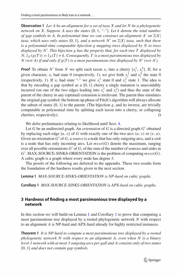
Given that each Ne contains 2 reticulations, there are 22 = 4 different switchings ofthese reticulations possible, shown in Fig. 2. Note that switchings 1 and 3 both induce5 mutations, while switchings 2 and 4 both induce 4 mutations. (Here by “inducemutations” we are referring to properties (i) and (ii) of Fitch’s algorithm, describedin the appendix). We now claim that there exists an optimum solution in which onlyswitchings 2 and 4 are used. Suppose, for some e = {u, v} ∈ E , switching 1 or 3 isused. Let T be the tree induced by this switching. Fix any optimal extension of A toT . Let Te be the subtree of T rooted at re; at least 5 mutations will be incurred onthe edges of Te (with respect to the extension; see property (i) of Fitch’s algorithm).Consider now the states allocated to re in columns u and v. There are four such uv

combinations: 00, 01, 10, 11. If it is combination 01 or 10, we could replace Te withthe subtree corresponding to switching 2 or 4 (respectively). This replacement subtreeincurs only 4 mutations on its edges, so the total number of mutations in T decreases.If it is combination 00 or 11 we can use switching 2. This might induce a newmutation(on the edge incoming to re) but we again save at least onemutation on the edges of thesubtree (because at most 4, rather than at least 5 mutations are incurred there), so the

123

Finding a most parsimonious or likely tree in a network. . .

∪∪{0,1}1

∪{0,1}{0,1}

{0,1}01{0,1} 0{0,1}

10xe,1

01xe,3

01xe,4

10xe,611

xe,2

00xe,5

Switching 15 mutations

∪∪

∪∪∪∪

{0,1}1

01

0{0,1}1{0,1} {0,1}0

10xe,1

01xe,3

01xe,4

10xe,611

xe,2

00xe,5

Switching 24 mutations

∪∪

∪∪1{0,1}

∪{0,1}{0,1}

0{0,1}{0,1}1 {0,1}0

10xe,1

01xe,3

01xe,4

10xe,611

xe,2

00xe,5

Switching 35 mutations

∪∪

∪∪1{0,1}

10

{0,1}0{0,1}1

0{0,1}

10xe,1

01xe,3

01xe,4

10xe,611

xe,2

00xe,5

Switching 44 mutations

Fig. 2 The four switchings possible for Ne . The interior nodes are labelled by the output of the bottom-upphase of Fitch’s algorithm, for the two characters concerned. The ∪ symbol denotes where union eventsoccur (i.e. mutations are incurred). The critical point is that both switching 2 and 4 incur the fewest numberof mutations, and these select for 01 and 10 at the root, respectively, representing the choice of which wayto orient edge e

overall number of mutations does not increase. Summarizing, whichever combination00, 01, 10, 11 occurs at re, we can replace it with switching 2 or 4 without increasingthe total number of mutations. Iterating this procedure proves the claim. Henceforthwe can thus assume that for each e ∈ E either switching 2 or 4 is used.

Observe that if, for a given e = {u, v}, the network Ne uses switching 2, thebottom-up phase of Fitch’s algorithm will allocate 01 (in columns u and v) to re. If, onthe other hand, switching 4 is used, Fitch’s algorithm will allocate 10. In both cases,exactly 4 union events are generated on the nodes (of the subtree of Ne induced by theswitching). See Fig. 2 for elucidation.

The central idea is that, since, for an edge e = {u, v}, a state 0 (resp. 1) in v

implies a state 1 (resp. 0) in u and vice versa, we can use the choice of whether to useswitching 2 or 4 (for each of the |E | reticulation pairs) to encode a choice as to whichway to orient the corresponding edge. Without loss of generality we use state 0 todenote incoming edges, and state 1 to denote outgoing edges. Consider the bottom-upphase of Fitch’s algorithm. Observe that, if a vertex v incident to three edges e1, e2, e3becomes a sink, the states at the roots of Ne1, Ne2 , Ne3 (in column v) will all be 0,and for each e′ /∈ {e1, e2, e3} the states at the root of Ne′ (in column v) will be “-”i.e. “don’t care”2. Continuing Fitch’s algorithm along the backbone of the caterpillar

2 Fitch’s algorithm is not well-defined on “-” symbols, but the intuition is that it behaves exactly like thesubset of states {0, 1} behaves in Fitch’s algorithm. This, in fact, is exactly how the construction describedin Observation 1 removes “-” symbols from the alignment.

123

S. Kelk et al.

shows that no mutations will be incurred on the edges of the caterpillar in column v. Acompletely symmetrical situation holds if a vertex becomes a source: the states at theroots of Ne1 , Ne2 , Ne3 (in column v) will all be 1, and again no mutations are incurredon the edges of the caterpillar. On the other hand, if a vertex v is neither a source nor asink, then the states assigned by the bottom-up phase of Fitch’s algorithm to the rootsof Ne1 , Ne2 , Ne3 (in column v) will consist of 0 (twice) and 1 (once) or 1 (twice) and0 (once). Either way exactly 1 mutation is then incurred on the edges of the caterpillar(as can be observed by running the top-down phase of Fitch’s algorithm).

This means that the parsimony score is minimized by creating as many sources andsinks as possible. Specifically we have

lA(N ) = 6|V | + (|V | − msso(G)).

Each edge in the graphwill induce 4mutations (within the Ne part), and |E | = 3|V |/2,which explains the term 6|V |. As argued above, sources and sinks to do not increasethe parsimony score, and all other vertices increase the parsimony score by exactly 1,hence the term (|V | − msso(G)).

Clearlymsso(G) can easily be calculated from lA(N ). Finally, we can apply Obser-vation 1 to obtain a network N ′ and A′ without “-” symbols such that

lA′(N ′) = 6|V |(|E | − 3) + 6|V | + (|V | − msso(G))

The transformation does not raise the level of the network or the number of arcsoutgoing from any biconnected component. NP-hardness follows. ��If we do allow “-” symbols then the following slightly stronger result is obtained:APX-hardness implies NP-hardness but additionally excludes the existence of a PolynomialTimeApproximationScheme (PTAS), unless P=NP.APX-hardness does not obviouslyhold ifwe encode the gap symbols usingObservation 1 because the additive O(|V ||E |)term thus created distorts the objective function.

Corollary 2 It is APX-hard to compute a most parsimonious tree displayed by a rootedphylogenetic network N with respect to an alignment A, even when N is a binarylevel-1 network with at most 3 outgoing arcs per gall and A consists only of states{0, 1, “-”}.Proof We give a (14, 1) L-reduction from msso, which is APX-hard, to the parsimonyproblem. L-reductions preserve APX-hardness so the result will follow. An (α, β) L-reduction (Papadimitriou andYannakakis 1991),whereα, β ≥ 0, is defined as follows.

Definition 1 Let A, B be two optimization problems and cA and cB their respectivecost functions.Apair of functions f , g, both computable in polynomial time, constitutean (α, β) L-reduction from A to B if the following conditions are true:

1. For every instance x of A, f (x) is an instance of B,2. For every feasible solution y of f (x), g(y) is a feasible solution of x ,3. For every instance x of A, O PTB( f (x)) ≤ αO PTA(x),

123

Finding a most parsimonious or likely tree in a network. . .

4. For every feasible solution y′ of f (x) we have |O PTA(x) − cA(g(y′))| ≤β|O PTB( f (x)) − cB(y′)|

where O PTA is the optimal solution value of problem A and similarly for B.

For brevity we refer to the optimum size of the parsimony problem as mp(N , A).We use the reduction described in the proof of Theorem 1 (before the gap symbolshave been removed) with some slight modifications. The forward-mapping function f(condition 1 of the L-reduction) is the same mapping used in the proof of Theorem 1.The back-mapping function g (i.e. condition 2) will be described below. To establishcondition 3 for a given (α, β) we need to prove that mp(N , A) ≤ α · msso(G). Now,we know thatmsso(G) = maxcut(G)−|V |/2 (see appendix) and thatmaxcut(G) ≥2/3|E | = |V | (because every cubic graph has a cut at least this large simply bymovingnodes which have more neighbours on their side of the cut, to the other side). Hence,msso(G) ≥ |V |/2. We know that mp(N , A) = 7|V | − msso(G). Trivially thereforemp(N , A) ≤ 7|V |. Hence taking α = 14 is sufficient. For the other direction, weneed to show that for an arbitrary solution to the parsimony problem, which inducesp mutations, the back-mapping function yields an orientation of G with s sources andsinks such that |msso(G) − s| ≤ β|p − mp(N , A)|. The back-mapping function gfirst ensures that all the Ne gadgets are using type 2 or type 4 switchings, which mightreduce the number of mutations to p′ ≤ p, and then extracts an orientation of G (thusestablishing condition 2). Now, s = 7|V | − p′ and mp(N , A) = 7|V | − msso(G) so

msso(G) − s = msso(G) − (7|V | − p′)= msso(G) − 7|V | + p′

= p′ − (7|V | − msso(G))

= p′ − mp(N , A)

≤ p − mp(N , A).

So taking β = 1 is sufficient to establish condition 4. ��

4 Hardness of finding amost likely tree displayed by a network

The likelihood of a tree. We now introduce the basic concepts and notation that arenecessary to define the likelihood of a tree with respect to an alignment. We largelyfollow the simple formulation by Roch (2006). First, we need a probabilistic modeldescribing how sequences evolve along a tree. Here we assume the simplest modelavailable, known as the Cavender-Farris model (Farris 1973; Cavender 1978), whichcan be described as follows. Let T = (V , E) be a rooted binary phylogenetic tree onX . We associate probabilities p = (pe)e∈E ∈ [0, 1/2]|E | to the edges of T and denotethis (T ,p). Under the Cavender-Farris model, each character evolves independently,as follows: at the root pick randomly a state between 0 and 1, each with probability1/2, and then, for each vertex v below the root, either copy the state of the parent ofv or flip it, with probabilities 1 − pe and pe, respectively. The restriction pe ≤ 1/2

123

S. Kelk et al.

corresponds to the fact that, in a symmetric model, no amount of time can make acharacter more likely to change state than to remain in the same state.

The process described above eventually associates a state to each element of X atthe leaves of the tree, that is, it generates a random binary character. The probabilityof generating the binary character f is called the likelihood of (T ,p) with respect tof , denoted L f (T ,p), and can be calculated as follows:

L f (T ,p) =∑

f

1

2

∏

e=(u,v)∈E

p| f (v)− f (u)|e (1 − pe)

1−| f (v)− f (u)|

Here f ranges over all extensions of f to T . Because the model assumes that thecharacters in a sequence evolve independently, the probability of generating the binarysequences in an alignment A, named the likelihood of (T ,p)with respect to A, denotedL A(T ,p), can be obtained as

L A(T ,p) =∏

f ∈A

L f (T ,p)

(Here, and in the rest of this section, we assume that alignments do not contain gapsymbols.)

We now introduce some more notation that will be useful in the following. Anextension A of an alignment A to a tree T = (V , E) is a set of functions f : V →{0, 1} obtained by taking exactly one extension of each character in A. In practice,A can be represented as a matrix with |V | rows and |A| columns, in which the rowscorresponding to the leaves of T are identical to the rows of A. For e = (u, v) ∈ E , wedenote by he( A) the number of differences (that is, the Hamming distance) betweenthe sequences that A associates to u and v. Finally, let l A(T ) denote

∑e∈E he( A) =∑

f ∈ A l f (T ). Note that the parsimony score lA(T ) is the minimum of l A(T ) over allextensions of A. Given these notations, we can express the likelihood of (T ,p) asfollows, where m = |A| = | A|, and A ranges over all extensions of A:

L A(T ,p) =∑

A

2−m∏

e∈E

phe( A)e (1 − pe)

m−he( A) (1)

Each term in the sum in Eqn. (1) expresses the product of the probabilities of transi-tion between the sequences associated by A to the endpoints of the edges, times theprobability of the sequence at the root.

Networks with edge probabilities. It is possible to extend the Cavender-Farris modelto describe the evolution of binary sequences on a binary rooted network N . For everyedge e of N , we define a probability p′

e ∈ [0, 1/2]which represents again the probabilityof change between 0 and 1 along edge e. The evolution of a single character followsthe same rules as in the case of a tree, except that when setting the state at a reticulationvertex v, one of its two parents is randomly selected with a probability γv ∈ (0, 1) (and1 − γv for the other parent), also given as a parameter of the model. The state at v isgenerated as if the selected parent of vwere the only parent of v, as in the tree case. That

123

Finding a most parsimonious or likely tree in a network. . .

v

w

a b c d e

0.2

0.10.1

0.3

0.1

0.1

0.10.2

00

0.10.2 0.2

0.3

v

w

v2v1

a b c d e

0.20.1 0.1

0.3

0.1

0.1

0.10.2

0.10.2 0.2

0.3

Fig. 3 Alternative representations of a phylogenetic network having some reticulation edges with strictlypositive lengths. A reticulation edge with positive length should be interpreted as ending in a node thatundergoes a reticulation event, but leaves no descendant in the network, other than the reticulation nodeitself. Both edges entering node v in the network on the left are an example of this. The representationon the right, which strictly speaking is not a phylogenetic network, makes the biological interpretation ofthese edges explicit. In this representation, dashed edges denote an instantaneous event, and their length isnecessarily 0 (not shown)

includes taking into account the probability of change p′e along the edge connecting

the selected parent to v. The inheritance probability parameters γv (e.g. Yu et al. 2012;Wen et al. 2016; Zhang et al. 2017), and mechanisms to correlate inheritance betweenneighboring characters in a sequence will not be discussed in the remainder of thispaper. These aspects of themodel are necessary to define the likelihood of the network,but they are irrelevant for the likelihood of the trees displayed by the network, which isall that concerns us here. In the following, we denote a network N and the probabilitiesof change along its edges as (N ,p′).

We note that in some cases, the edges entering a reticulation node (the reticulationedges) may represent an event of instantaneous combination between the sequencesat the tails of the reticulation edges. The probabilities of change p′

e for these reticula-tion edges will necessarily equal 0, as they represent an immediate transfer of geneticinformation, and there is no time for sequence changes along these edges. The edgesentering node w in the network of Fig. 3 are an example of this. Not all edges enteringa reticulation, however, need be of this type. For the sake of generality, the networkswe consider here may have “non-istantaneous” reticulation edges, that is reticulationedges with p′

e > 0. For example, consider the edges entering node v in the networkof Fig. 3. Edges like these simply mean that before the reticulate event happened,the sequence in the edge leading to the reticulation evolved independently of the restof the tree, potentially accumulating changes. At the end of the edge, the sequencethat underwent the reticulate event left no descendant leading to a leaf, other thanthe sequence at the reticulation itself. Figure 3 also displays a different representa-tion of the same network, showing separately the nodes v1 and v2 that underwent thereticulation event. Neither of these nodes left any other descendant than v within thenetwork. In somebiological contexts (for examplewhen reticulations represent homol-ogous recombinations), reticulation edges representing lineages that have existed for astrictly positive amount of time are the norm, and not the exception. Examples of thisare the phylogenetic networks generated by the coalescent with recombination model(e.g. Griffiths and Marjoram 1997; Nordborg 2001), or by the birth-hybridization

123

S. Kelk et al.

a b c d e

0.180.26

0.32

0.2

0.3

0.1

0.1

0.3

a b c d e

0.18

0.18

0.2 0.20.2

0.3

0.1

0.3

a b c d e

0.26

0.38

0.18 0.2

0.2

0.1

0.1

0.3

a b c d e

0.1

0.1

0.380.356

0.2 0.2

0.1

0.3

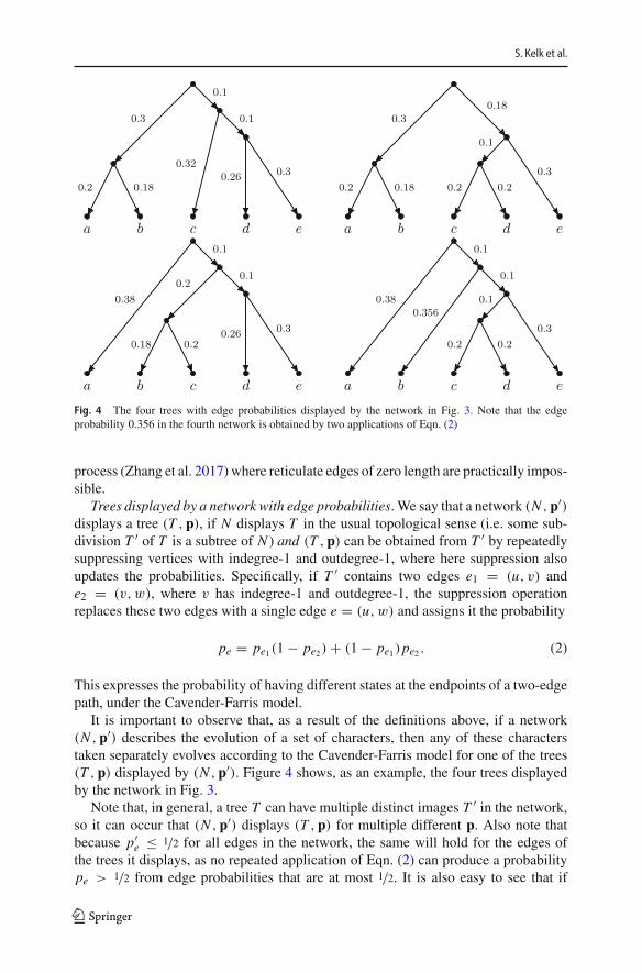
Fig. 4 The four trees with edge probabilities displayed by the network in Fig. 3. Note that the edgeprobability 0.356 in the fourth network is obtained by two applications of Eqn. (2)

process (Zhang et al. 2017) where reticulate edges of zero length are practically impos-sible.

Trees displayed by a network with edge probabilities. We say that a network (N ,p′)displays a tree (T ,p), if N displays T in the usual topological sense (i.e. some sub-division T ′ of T is a subtree of N ) and (T ,p) can be obtained from T ′ by repeatedlysuppressing vertices with indegree-1 and outdegree-1, where here suppression alsoupdates the probabilities. Specifically, if T ′ contains two edges e1 = (u, v) ande2 = (v,w), where v has indegree-1 and outdegree-1, the suppression operationreplaces these two edges with a single edge e = (u, w) and assigns it the probability

pe = pe1(1 − pe2) + (1 − pe1)pe2 . (2)

This expresses the probability of having different states at the endpoints of a two-edgepath, under the Cavender-Farris model.

It is important to observe that, as a result of the definitions above, if a network(N ,p′) describes the evolution of a set of characters, then any of these characterstaken separately evolves according to the Cavender-Farris model for one of the trees(T ,p) displayed by (N ,p′). Figure 4 shows, as an example, the four trees displayedby the network in Fig. 3.

Note that, in general, a tree T can have multiple distinct images T ′ in the network,so it can occur that (N ,p′) displays (T ,p) for multiple different p. Also note thatbecause p′

e ≤ 1/2 for all edges in the network, the same will hold for the edges ofthe trees it displays, as no repeated application of Eqn. (2) can produce a probabilitype > 1/2 from edge probabilities that are at most 1/2. It is also easy to see that if

123

Finding a most parsimonious or likely tree in a network. . .

0 < pe1, pe2 < 1/2, then max{pe1, pe2} < pe < pe1 + pe2 . These observations leadto the following one, which will be useful later on:

Observation 2 Let (N ,p′) be such that for every edge of N , 0 < p′e < 1/2. Let (T ,p)

be a tree displayed by (N ,p′) and e an edge of T . Finally, let E ′(e) be the subset ofthe edges of N whose probabilities contribute to pe. Then, pe < 1/2 and

maxe′∈E ′(e)

pe′ < pe <∑

e′∈E ′(e)pe′

We say that (T ∗,p∗) is a most likely (ML) tree displayed by (N ,p′) (with respectto A) if it maximizes L A(T ,p), ranging over all (T ,p) displayed by (N ,p′). In theremainder of this section we consider the problem of finding such a most likely treegiven a network with edge probabilities and an alignment.

A link between likelihood and parsimony. There are well-known relationshipsbetween the likelihood and the parsimony of a tree that imply that under some con-ditions a most likely tree is also a most parsimonious one (Tuffley and Steel 1997).We now illustrate one such relationship (Corollary 3 below), which is based on theobservation that as we reduce the scale of a tree, its likelihood converges to zero at arate that only depends on its parsimony score. Although it shares similarities with theresults by Tuffley and Steel, we are not aware that it has been explicitly stated in theliterature. This result is not necessary to obtain the other results in this section, but itprovides the intuition behind them.

In the following statements, we assume that c ∈ (0, 1), so the form c → 0 is tobe understood as c approaches 0 to the right. Also, cp simply denotes the productbetween the scalar c and vector p.

Lemma 2 The function f (c) = L A(T , cp) is �(clA(T )) as c → 0.

Proof Write L A(T , cp) using Eqn. (1):

L A(T , cp) =∑

A

2−m∏

e∈E

(cpe)he( A)(1 − cpe)

m−he( A)

=∑

A

2−mclA(T ) ·∏

e∈E

phe( A)e (1 − cpe)

m−he( A),

where we have used∑

e∈E he( A) = l A(T ). Note that the products in the secondexpression tend to a constant as c → 0. As a consequence, the term for A in thesum has order �(clA(T )) as c → 0. Since the lowest degree dominates, their sum is�(clA(T )). ��Corollary 3 Let A be an alignment and T1 and T2 two trees such that lA(T1) < lA(T2).Then, for any p1 and p2,

L A(T1, cp1) > L A(T2, cp2) for c sufficiently close to 0.

123

S. Kelk et al.

Proof As c → 0, L A(T1, cp1) is �(clA(T1)), while L A(T2, cp2) is �(clA(T2)). Thatis, L A(T1, cp1) converges to 0 at a lower rate than L A(T2, cp2). Thus there exists aneighborhood of 0 in which L A(T1, cp1) > L A(T2, cp2) holds. ��

The corollary above can be extended to any collection of trees: irrespective of theedge probabilities assigned to them, if the trees are rescaled by a sufficiently smallc, the most parsimonious trees will have likelihoods greater than all the other trees,meaning that a most likely tree in the collection of rescaled trees will necessarily alsobe most parsimonious.

Proving the NP-hardness of finding an ML tree in a network. In the remainder ofthis section, namely in the statements of the next two formal results, we are implicitlygiven a network N on X with |X | = n and an alignment A with m characters on X .The height of a network N is the maximum number of edges in a directed path in N .

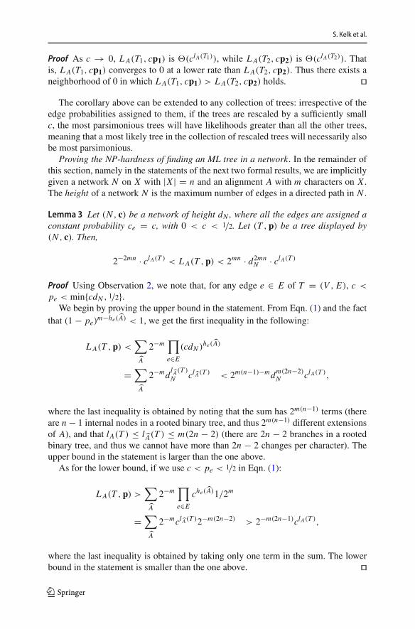
Lemma 3 Let (N , c) be a network of height dN , where all the edges are assigned aconstant probability ce = c, with 0 < c < 1/2. Let (T ,p) be a tree displayed by(N , c). Then,

2−2mn · clA(T ) < L A(T ,p) < 2mn · d2mnN · clA(T )

Proof Using Observation 2, we note that, for any edge e ∈ E of T = (V , E), c <

pe < min{cdN , 1/2}.We begin by proving the upper bound in the statement. From Eqn. (1) and the fact

that (1 − pe)m−he( A) < 1, we get the first inequality in the following:

L A(T ,p) <∑

A

2−m∏

e∈E

(cdN )he( A)

=∑

A

2−mdlA(T )

N clA(T ) < 2m(n−1)−mdm(2n−2)N clA(T ),

where the last inequality is obtained by noting that the sum has 2m(n−1) terms (thereare n − 1 internal nodes in a rooted binary tree, and thus 2m(n−1) different extensionsof A), and that lA(T ) ≤ l A(T ) ≤ m(2n − 2) (there are 2n − 2 branches in a rootedbinary tree, and thus we cannot have more than 2n − 2 changes per character). Theupper bound in the statement is larger than the one above.

As for the lower bound, if we use c < pe < 1/2 in Eqn. (1):

L A(T ,p) >∑

A

2−m∏

e∈E

che( A)1/2m

=∑

A

2−mclA(T )2−m(2n−2) > 2−m(2n−1)clA(T ),

where the last inequality is obtained by taking only one term in the sum. The lowerbound in the statement is smaller than the one above. ��

123

Finding a most parsimonious or likely tree in a network. . .

The lemma above shows the order of convergence to 0 of the likelihood L A(T ,p)

of a tree displayed by (N , c) as c → 0. The higher the parsimony score, the fasterthe convergence. As a consequence, for c sufficiently close to 0, a tree with a lowerparsimony score than another will have a higher likelihood. The following lemmashows how close is “sufficiently close”, by providing an explicit upper bound to c.

Proposition 1 Let (N , c) be a network of height dN , where all the edges are assigneda constant probability ce = c, with 0 < c < d−2mn

N 2−3mn. If (T ∗,p∗) is a most likelytree displayed by (N , c), then T ∗ is a most parsimonious tree displayed by N. ��Proof Suppose that (T ∗,p∗) is a most likely tree displayed by (N , c), but not mostparsimonious. That is, there exists (T ,p)displayed by (N , c)with lA(T ) ≤ lA(T ∗)−1.But then, by using the lower bound in Lemma 3:

L A(T ,p) > 2−2mn · clA(T ) ≥ 2−2mn · clA(T ∗)−1.

Now apply the upper bound in Lemma 3 to T ∗, and combine it with c < d−2mnN 2−3mn :

L A(T ∗,p∗) < 2mn · d2mnN · clA(T ∗) < 2mn · d2mn

N · clA(T ∗)−1 · d−2mnN · 2−3mn

= 2−2mn · clA(T ∗)−1

The last terms of the two chains of inequalities above are equal, thus provingL A(T ,p) > L A(T ∗,p∗). Since this contradicts the assumption that (T ∗,p∗) is amost likely tree, the statement follows. ��

The proposition above shows that the NP-hard problem of finding a most parsimo-nious tree in a network N with respect to an alignment A can be reduced to the problemof finding a most likely tree in (N , c) with respect to A, where c = (ce) is such thatce = c, and 0 < c < d−2mn

N 2−3mn . Since the reduction preserves the network and thealignment, the main result of this section follows from Theorem 1:

Theorem 2 It is NP-hard to compute a most likely tree (T ,p) displayed by a rootedphylogenetic network (N ,p′) with respect to an alignment A, even when N is a binarylevel-1 network with at most 3 outgoing arcs per gall and A consists only of two states{0, 1} and does not contain gap symbols.

5 Conclusions and open problems

We have shown that, given a phylogenetic network with a sequence for each leaf,finding a most parsimonious or most likely tree displayed by the network is compu-tationally intractable (NP-hard). Moreover, this is the case even when we restrict tobinary sequences and level-1 networks; the simplest networks that are not trees. How-ever, many computational problems that can be shown to be theoretically intractablecan be solved reasonably efficiently in practice (see e.g. Cautionary Tales of Inap-proximability by Budden and Jones (2017)). We end the paper by discussing whetherwe expect this to be the case for our problem.

123

S. Kelk et al.

There is a dynamic programming algorithm, described in Theorem 5.7 of Fischeret al. (2015), for finding a tree in a network that is most parsimonious with respect toa single character. The running time is fixed-parameter tractable, with as parameterthe level of the network. Hence, this algorithm is practical as long as the level of thenetwork is not too large. This algorithm can easily be extended to multiple characters(that all have to choose the same tree) when the number of characters is adopted as asecond parameter. Indeed, for every root of a biconnected component, we introducea dynamic programming entry not just for every possible state but for every possiblesequence of states. However, the running time of this algorithm would be exponentialin the number of characters, which makes it useless for almost all biological data.Similarly, the Integer Linear Programming (ILP) solution presented in the same papercan also be easily extended to multiple characters. However, there does not seem to bean easy way to do that without having the number of variables growing linearly in thenumber of characters. Hence, this approach is also unlikely to be useful in practice.

In contrast, consider the simple algorithm that loops through the at most 2r treesdisplayed by the network, with r the number of reticulation nodes in the network,and computes the parsimony or likelihood of each tree (this naïve FPT algorithmwas presented in Nakhleh et al. (2005), where it is named Net2Trees). Ironically, thissimple algorithm would outperform the approaches mentioned above for any kind ofdata with a reasonably large number of characters. Hence, the main open questionthat remains is whether there exists an algorithm whose running time is linear (or atleast polynomial) in the number of characters and whose dependency on r is betterthan 2r (for example recently an algorithm with exponential base smaller than 2 wasdiscovered for the tree containment problem (Gunawan et al. 2016), although thisalgorithm does not obviously extend to generating all trees in the network). Anotherquestion of interest that remains open is the following: does the parsimony problemunder restrictions (1)-(3) listed in the introduction permit good (i.e. constant factor)approximation algorithms, and possibly even a PTAS, when the alignment A does notcontain any indels?

Acknowledgements Leo van Iersel was partly supported by the Netherlands Organization for ScientificResearch (NWO), including Vidi grant 639.072.602, and partly by the 4TU Applied Mathematics Institute.Celine Scornavacca was partly supported by the French Agence Nationale de la Recherche Investissementsd’Avenir/Bioinformatique (ANR-10-BINF-01-02, Ancestrome).

Open Access This article is distributed under the terms of the Creative Commons Attribution 4.0 Interna-tional License (http://creativecommons.org/licenses/by/4.0/), which permits unrestricted use, distribution,and reproduction in any medium, provided you give appropriate credit to the original author(s) and thesource, provide a link to the Creative Commons license, and indicate if changes were made.

A Appendix: Fitch’s algorithm

Fitch’s algorithm (Fitch 1971) has two phases. In the first phase, known as the bottom-up phase, we start by assigning the singleton subset of states { f (x)} to each taxon x .The internal nodes of T are assigned subsets of states recursively, as follows. Supposea node p has two children u and v, and the bottom-up phase has already assignedsubsets F(u) and F(v) to the two children, respectively. If F(u) ∩ F(v) �= ∅ then

123

Finding a most parsimonious or likely tree in a network. . .

set F(p) = F(u) ∩ F(v) (in which case we say that p is an intersection node). IfF(u) ∩ F(v) = ∅ then set F(p) = F(u) ∪ F(v) (in which case we say that p is aunion node). The number of union nodes in the bottom-up phase is equal to l f (T ).To actually create an optimal extension f , we require the top-down phase of Fitch’salgorithm. Start at the root r and let f (r) be any element in F(r). For an internalnode u with parent p, we set f (u) = f (p) (if f (p) ∈ F(u)) and otherwise (i.e.f (p) /∈ F(u)) set f (u) to be an arbitrary element of F(u).For each node u of the tree, let ∪(u) be the number of union events in the sub-

tree rooted at u. The following well-known properties of Fitch’s algorithm are usedrepeatedly in the main hardness proof of this article: (i) every extension (optimal orotherwise) must incur at least ∪(u) mutations on the edges of the subtree rooted at u;(ii) an extension created by Fitch’s algorithm induces exactly ∪(u) mutations on theedges of the subtree rooted at u (and u is assigned a state from F(u) in this extension).

B Appendix: NP-hardness and APX-hardness ofMAX-SOURCE-SINKS-ORIENTATION

The following result is based on a sketch proof by Colin McQuillan3. We have beenunable to find an original reference and hence have reconstructed the proof in detail.The APX-hardness proof is original.

Lemma 1. MAX-SOURCE-SINKS-ORIENTATION is NP-hard on cubic graphs.

Proof Recall that the classical MAX-CUT problem asks us to bipartition the vertexset of an undirected graph G, such that the number of edges that cross the bipartitionis maximized. We reduce from the NP-hard problem CUBIC-MAX-CUT which is therestriction of theMAX-CUTproblem to cubic graphs.Given an undirected cubic graphG, we simply write maxcut(G) to denote the number of edges in the maximum-sizecut.

We reduceCUBIC-MAX-CUT toMAX-SOURCE-SINKS-ORIENTATION.Specif-ically, given an undirected cubic graph G = (V , E) (i.e. an instance of CUBIC-MAX-CUT) we will show that msso(G) = maxcut(G) − |V |/2, from which the hardnesswill follow.

We start by proving that msso(G) ≥ maxcut(G) − |V |/2. Fix an arbitrary cut Cof G and let (U , W ) be the corresponding bipartition. If some vertex of U or W hasmore neighbours on the other side of the partition than its own, move it to the otherside of the partition: this will increase the size of the cut. We repeat this until it isno longer possible and let C and (U , W ) refer to the cut and its induced partition atthe end of this process. Note that now each vertex in U (respectively, W ) will haveat most one neighbour in U (respectively, W ). We proceed by orienting the edges inthe cut from U to W . Now, the remaining edges are either internal to U or internalto W . These edges must form a matching (i.e. they are node disjoint). For each such

3 TCS Stack Exchange, 2010, URL: http://cstheory.stackexchange.com/questions/2307/an-edge-partitioning-problem-on-cubic-graphs/.

123

S. Kelk et al.

edge in U (respectively, W ), exactly one endpoint will become a source (respectively,sink). Nodes in U (respectively, W ) that are not adjacent to internal edges will alreadybe sources (respectively, sinks) due to the orientation of the cut edges from U to W .Hence, if we write |C | to denote the number of edges in the cut C , we obtain anorientation of G with at least

(|E | − |C |) + (|V | − 2(|E | − |C |))

sources and sinks. Hence,

msso(G) ≥ (|E | − maxcut(G)) + (|V | − 2(|E | − maxcut(G)))

= maxcut(G) + |V | − |E |= maxcut(G) + |V | − (3/2)|V |= maxcut(G) − |V |/2.

For the other direction, fix an arbitrary orientation of G and let s be the number ofsources and sinks created by the orientation. We write Vi (i ∈ {0, 1, 2, 3}) to denotethose vertices of G which have indegree i . Let U = V0 ∪ V1 and let W = V2 ∪ V3.Whenever an edge of G has been oriented from W to U , reverse its orientation: thisonly decreases the indegrees of the vertices inU and increases the indegrees of verticesin W so it cannot destroy any sources or sinks and it cannot cause a node to be on the“wrong” side of the bipartition. (In fact, it will cause the number of sources and sinksto increase, so this situation can only occur if the orientation was not optimal). Let snow refer to the number of sources and sinks once all arcs have been oriented fromU to W . The edges (u, w) such that u ∈ U and w ∈ W form a cut; it remains only tocount how many of these edges there are. We first count from the perspective of thevertices inU . The nodes in V0 each generate 3 outgoing arcs. Let k be the total numberof edges of the form (u0, u1) where u0 ∈ V0 and u1 ∈ V1. Note that each node in V1that does not receive any of these k arcs, must receive an arc which is outgoing fromsome other node in V1. It follows that the number of edges in the cut is

(3|V0| − k) + (2|V1| − (|V1| − k)) = 3|V0| + |V1|.

If we count in a symmetrical fashion from the perspective of W , and let � be thenumber of arcs of the form (u2, u3) where u2 ∈ V2 and u3 ∈ V3, it follows that thenumber of edges in the cut is

(3|V3| − �) + (2|V2| − (|V2| − �)) = 3|V3| + |V2|.

If we sum these two equations, we obtain a cut with at least the following number ofedges:

≥ (3/2)(|V0| + |V3|) + (1/2)(|V1| + |V2|)= (3/2)s + (1/2)(|V | − s)

= s + (1/2)|V |.

123

Finding a most parsimonious or likely tree in a network. . .

From this follows that msso(G) ≤ maxcut(G) − (1/2)|V |. ��The hardness ofmsso can be strengthened to the following inapproximability result.

Note that one consequence of APX-hardness is that msso does not permit a PTAS,unless P = N P .

Corollary 1 MAX-SOURCE-SINKS-ORIENTATION is APX-hard on cubic graphs.

Proof Note that the constructions and transformations used in the proof of Lemma 1are all constructive and can easily be conducted in polynomial time. Moreover, theyapply to arbitrary cuts/orientations, and not just optimal ones. This allows us to easilystrengthen the described reduction to obtain a (1, 1) L-reduction from CUBIC-MAX-CUT toMAX-SOURCE-SINKS-ORIENTATION (see the main text for the definitionof L-reduction). From this APX-hardness will follow, since CUBIC-MAX-CUT isAPX-hard (Alimonti and Kann 1997; Berman and Karpinski 1999) and L-reductionsare APX-hardness preserving. The (1, 1) means that the inapproximability threshholdfor MAX-SOURCE-SINKS-ORIENTATION is at least as strong as that for CUBIC-MAX-CUT.

Let G = (V , E) be an instance of CUBIC-MAX-CUT. The forward mappingfunction f (from instances of CUBIC-MAX-CUT to MAX-SOURCE-SINKS-ORIENTATION) is simply the identity function. To be an (α, β) L-reduction, whereα, β ≥ 0, we first have to show that msso( f (G)) = msso(G) ≤ α · maxcut(G).We know that maxcut(G) − (1/2)|V | = msso(G), so α = 1 is trivially satisfied.We next have to show a polynomial-time computable back-mapping function g (fromfeasible solutions ofMAX-SOURCE-SINKS-ORIENTATION to feasible solutions ofCUBIC-MAX-CUT)with the following property: an orientation that induces s sourcesand sinks ismapped to a cutwith k edges such that |maxcut(G)−k| ≤ β|msso(G)−s|.The function g was already implicitly described in the NP-hardness reduction: reverseany edges oriented from W to U (which possibly increases the number of sources andsinks to s′ ≥ s) and extract a cut of size s′ + |V |/2. Observe,

maxcut(G) − (s′ + |V |/2) ≤ maxcut(G) − (s + |V |/2)≤ (msso(G) + |V |/2) − (s + |V |/2)≤ msso(G) − s.

So taking β = 1 is sufficient. ��

References

Abbott R, Albach D, Ansell S, Arntzen JW, Baird SJ, Bierne N, Boughman J, Brelsford A, Buerkle CA,Buggs R (2013) Hybridization and speciation. J Evol Biol 26(2):229–246

Alimonti P, Kann V (1997) Hardness of approximating problems on cubic graphs. In: Italian conference onalgorithms and complexity (CIAC), pp 288–298

Berman P, Karpinski M (1999) On some tighter inapproximability results (extended abstract). In: Inter-national Colloquium on automata, languages and programming (ICALP), Lecture notes in computerscience, vol 1644, pp 200–209

Budden D, Jones M (2017) Cautionary tales of inapproximability. J Comput Biol 24(3):213–216

123

S. Kelk et al.

Cavender JA (1978) Taxonomy with confidence. Math Biosci 40(3–4):271–280Fakcharoenphol J, Kumpijit T, Putwattana A (2015) A faster algorithm for the tree containment problem for

binary nearly stable phylogenetic networks. In: 2015 12th international joint conference on computerscience and software engineering (JCSSE), IEEE, pp 337–342

Farris JS (1973) A probability model for inferring evolutionary trees. Syst Biol 22(3):250–256Fischer M, Van Iersel L, Kelk S, Scornavacca C (2015) On computing the maximum parsimony score of a

phylogenetic network. SIAM J Discret Math 29(1):559–585Fitch W (1971) Toward defining the course of evolution: minimum change for a specific tree topology. Syst

Biol 20(4):406–416Gambette P, Gunawan AD, Labarre A, Vialette S, Zhang L (2015) Locating a tree in a phylogenetic network

in quadratic time. In: RECOMB, pp 96–107Griffiths RC, Marjoram P (1997) An ancestral recombination graph. In: Donelly P, Tavaré S (eds) Progress

in population genetics and human evolution. Springer, Berlin, pp 257–270Gunawan AD, Lu B, Zhang L (2016) A program for verification of phylogenetic network models. Bioin-

formatics 32(17):i503–i510Gusfield D (2014) ReCombinatorics: the algorithmics of ancestral recombination graphs and explicit phy-

logenetic networks. MIT Press, CambridgeHein J (1990)Reconstructing evolution of sequences subject to recombination using parsimony.MathBiosci

98(2):185–200Huson DH, Rupp R, Scornavacca C (2010) Phylogenetic networks: concepts, algorithms and applications.

Cambridge University Press, CambridgeJin G, Nakhleh L, Snir S, Tuller T (2006) Maximum likelihood of phylogenetic networks. Bioinformatics

22(21):2604–2611Jin G, Nakhleh L, Snir S, Tuller T (2007) Efficient parsimony-based methods for phylogenetic network

reconstruction. Bioinformatics 23(2):e123–e128Kanj IA, Nakhleh L, Than C, Xia G (2008) Seeing the trees and their branches in the network is hard. Theor

Comput Sci 401(1–3):153–164Kannan L, Wheeler WC (2012) Maximum parsimony on phylogenetic networks. Algorithms Mol Biol

7(1):9Kelk S, Scornavacca C (2014) Constructing minimal phylogenetic networks from softwired clusters is fixed

parameter tractable. Algorithmica 68(4):886–915Morrison D (2011) Introduction to phylogenetic networks. RJR Productions, UppsalaNakhlehL, JinG, ZhaoF,Mellor-Crummey J (2005)Reconstructing phylogenetic networks usingmaximum

parsimony. In: Computational systems bioinformatics conference, 2005. Proceedings. 2005 IEEE,IEEE, pp 93–102

Nordborg M (2001) Coalescent theory. In: Balding, DJ , Bishop, M and Cannings, Christopher, Wiley,Hoboken

Papadimitriou CH, Yannakakis M (1991) Optimization, approximation, and complexity classes. J ComputSyst Sci 43:425–440

Roch S (2006) A short proof that phylogenetic tree reconstruction by maximum likelihood is hard.IEEE/ACM Trans Comput Biol Bioinform 3(1):92–94

Tuffley C, Steel M (1997) Links between maximum likelihood and maximum parsimony under a simplemodel of site substitution. Bull Math Biol 59(3):581–607

Van Iersel L, Semple C, Steel M (2010) Locating a tree in a phylogenetic network. Inf Process Lett110(23):1037–1043

van Iersel L, Jones M, Scornavacca C (2018) Improved maximum parsimony models for phylogeneticnetworks. Syst Biol 67(3):518–542

Vuilleumier S, Bonhoeffer S (2015) Contribution of recombination to the evolutionary history of hiv. CurrOpin HIV AIDS 10(2):84–89

WenD,YuY,Nakhleh L (2016)Bayesian inference of reticulate phylogenies under themultispecies networkcoalescent. PLoS Genet 12(5):e1006,006

Yu Y, Degnan J, Nakhleh L (2012) The probability of a gene tree topology within a phylogenetic networkwith applications to hybridization detection. PLoS Genet 8(4):e1002,660

Zhang C, Ogilvie HA, Drummond AJ, Stadler T (2017) Bayesian inference of species networks frommultilocus sequence data. Mol Biol Evol 35(2):504–517

Zhaxybayeva O, Doolittle WF (2011) Lateral gene transfer. Curr Biol 21(7):R242–R246

123

Finding a most parsimonious or likely tree in a network. . .

Affiliations

Steven Kelk1 · Fabio Pardi2 · Celine Scornavacca3 · Leo van Iersel4

B Steven Kelksteven.kelk@maastrichtuniversity.nl

Fabio Pardipardi@lirmm.fr

Celine Scornavaccaceline.scornavacca@umontpellier.fr

Leo van Iersell.j.j.v.iersel@gmail.com

1 Department of Data Science and Knowledge Engineering (DKE), Maastricht University, P.O.Box 616, 6200 MD Maastricht, The Netherlands

2 LIRMM, Université de Montpellier, CNRS, Montpellier, France

3 Institut des Sciences de l’Evolution, CNRS, IRD, EPHE, Institut de Biologie Computationnelle(IBC), Université de Montpellier, 34095 Montpellier Cedex 5, France

4 Delft Institute of Applied Mathematics, Delft University of Technology, Van MourikBroekmanweg 6, 2628 XE Delft, The Netherlands

123