PO

LIT

ICA

L E

CO

NO

MY

R

ESEA

RC

H IN

ST

ITU

TE

 

Financialization and the Rise in

Comovement of Commodity Prices

Manisha Pradhananga

February 2015

WORKINGPAPER SERIES

Number 376

1

Financialization and the Rise in Comovement of Commodity Prices

Manisha Pradhananga1 Abstract: Between January 2000 and June 2008, the FAO food price index rose by 96 percent. Besides the magnitude, the price rise was remarkable for the broad range of commodities affected; prices of agriculture commodities, energy, and metals all rose and fell together. These dramatic developments coincided with the rise of commodities as an asset class. In this paper, I study the causal links between the increase in comovement between commodity prices and this financialization of the commodities futures market. I extract common factors from a group of 41 commodities using the PANIC method and include it in a factor-augment VEC model along with a proxy of financialization. Results from the empirical analysis show that financialization of the commodities futures markets led to the recent rise in comovement between commodity prices. 1. Introduction After declining for almost three decades, the food price index of the Food and Agricultural Organization (FAO) rose by 96 percent in real terms, between January 2000 and June 2008. Prices then dropped precipitously only to reach new heights in February 2011. Besides the magnitude, the 2008-2011 commodity price developments were remarkable for the breadth of commodities affected – prices of a wide range of commodities including agricultural (wheat, corn, soybeans, cocoa, coffee), energy (crude oil, gasoline), and metals (copper, aluminum), all rose and fell together during this period.

Figure 1: Annual Food Price Index, 1990-2012 Source: FAO

1 Manisha Pradhananga is Assistant Professor of Economics at Knox College.

2

Prices of two commodities may move together, if they are related -- they are either complements or substitutes in production or consumption. Idiosyncratic demand or supply shocks in a particular commodity may be transmitted to other related commodities. However, commodity-specific shocks cannot explain recently observed broad co-movement across unrelated commodities. Commodity-specific shocks such as drought, use of corn and oil-seeds to produce biofuels that were initially provided as explanation for the 2008 rise in commodity prices, have now been questioned, as they are unable to explain this synchronized behavior across commodity prices (Gilbert 2010, Frankel and Rose 2009). Instead factors that can affect many commodity markets simultaneously are emphasized such as: rise in demand from emerging economies2 (Krugman 2008, Hamilton 2009), devaluation of the USD (Akram 2008), and financialization of the commodities futures market (Mayer 2009; Robles, Torero, and Braun 2009). In this paper, I examine if financialization of the commodity futures market can explain the recent rise in comovement in commodity prices. Following recent developments in the literature, I extract common factors from prices of 41 commodities using the Panel Analysis of Nonstationary and Idiosyncratic Components (PANIC) method of Bai and Ng (2004). The extracted factor is then included in a factor-augmented vector error-correction (FAVEC) model along with macroeconomic variables. Instead of assuming the excess comovement unexplained by macroeconomic factors is due to speculation, I add the sum of Open Interest across commodity markets, in terms of dollars and number of contracts, as measures of financialization in the FAVEC model. This will be a stronger and more direct evidence of the role of financialization in explaining comovement of commodity prices, than previously provided in the literature. Results show that both proxies of financialization are significant and have the expected signs; implying that comovement between commodity prices rise with market liquidity. This result provides strong evidence to support the thesis that financialization of the commodities futures market led to increasing comovement between unrelated commodity prices. The rest of the paper is organized as follows: In Section 2, I provide some background on financialization of the commodities market, followed by a brief literature review in Section 3. Section 4 contains details on the data and empirical strategy. In Section 5, I summarize the results of the empirical exercise, and finally conclude in Section 6. 2. Financialization of the commodities markets The term financialization has been used in the broader political economy literature to loosely describe a range of developments related to the rising dominance of financial markets, institutions, and interests in the US economy since the 1970s. Some have used the term to describe a pattern of accumulation in which profits of non-financial corporations accrue primarily through financial activities and channels rather than real productive activities; some focus on the growing importance of ‘shareholder value’ as

2 Ghosh (2010) argues that demand-supply shifts for food commodities, including due to the use of food commodities in biofuels, are not large enough in magnitude to explain the rise in magnitude and volatility of prices.

3

a mode of corporate governance; some use the term to refer to the rapid increase in financial trading and new financial products; while others refer to the increasing political and economic power of the rentier class (Epstein and Jayadev 2005, Orhangazi 2008). Pollin and Heintz (2012) further argue that the process of financialization has transformed the financial sector itself -- there has been a sharp decline in the role of traditional banks and other depository institutions as providers of credit, and a subsequent rise in “shadow banking.”3 This concept of financialization has been extended to the commodities markets, where financial actors and interests have similarly played an increasingly dominant role in the functioning of the market. Financialization in the context of the commodities futures market refers to the massive inflow of investment, and the rise of commodities as an investment asset. Interest in commodity futures rose after the collapse of the equity market in early-2000s when investors were looking for safe assets. Commodity futures were marketed by the financial industry and several academic economists4 as an asset class, with returns of a weighted index of commodities comparable to that of S&P500, but uncorrelated with stocks and bonds. Commodities were thus seen an effective way to diversify investment and hedge against inflation. Consequently, investment in commodity derivatives market, through both exchanges and over-the-counter (OTC) increased rapidly. According to the Bank of International Settlements (BIS), the total Open Interest 5 in US exchange-traded commodity derivatives market increased from around 6 million in 2001 to 37 million in June 2008, and to more than 50 million in 2011. Initially, a majority of investors gained exposure to commodities through managed funds that agree to mimic a popular commodity index benchmark such as the Standard and Poor-Goldman Sachs commodity index (S&P GSCI) and the Dow Jones-UBS (DJ-UBS) commodity index. 6 Large institutional investors like pension funds and university endowments have been especially active in this kind of passive investment strategies. In recent years, Exchange Traded Funds (ETFs) and Exchange Traded Notes (ETNs) have also gained popularity. Besides this quantitative change, the inflow of index traders changed the futures market qualitatively. Historically two types of traders have existed in the commodities futures market: “bonafide” hedgers -- producers and consumers of commodities who have commercial interest in the underlying commodities; and traditional speculators – traders who do not have any commercial interest in the physical commodities, and are in the market to profit from changes in futures prices. Commodity index traders (CITs), the new financial actors in the commodities futures market, have no interest in production, distribution, or consumption of the underlying commodities they are trading. However, unlike traditional speculators, index traders’ decisions are not based on individual commodity prices, but on prices of a broad range of commodities and other portfolio considerations. During 1995-2001, hedgers controlled 70 percent of the Open Interest in crude oil; by 2006-09 they controlled less than 43 percent, the

3 Pollin and Heintz (2012) define shadow banking as comprising of mutual funds, finance companies, real estate investment trusts, holding companies, hedge funds, private equity funds, and similar entities that began growing rapidly in the US in the 1980s. 4 For example see: Greer (2000), Gorton and Rouwenhorst (2004) 5 Open Interest is the total open contracts held by market participants at the end of the trading day. 6 S&P-GSCI and DJ-UBSCI hold over 63 percent and 32 percent of the market respectively.

4

rest controlled by traditional speculators and index traders.7 Financialization of commodity futures markets may cause co-movement between unrelated commodities in three ways. First, if commodity futures are bought and sold not based on commodity-specific demand and supply fundamentals, but based on other portfolio considerations or due to herd behavior. This is especially true for financial traders who buy and sell commodity derivatives not individually but as a group of securities based on pre-set weights of one of the popular commodity indices like the S&P GSCI and DJ-UBS commodity index. If a large portion of “investment” in the commodities derivatives market are controlled by such passive index trading (like they did in 2008), then it is likely that prices of commodities will move together. Second, if commodity speculators trade in two or more commodity markets, a fall in the price of one commodity may cause the price of other commodity to also fall due to liquidity effects. For example, if price of commodity A rises, speculators might have to sell commodity B to cover margin calls in commodity A in which they are long, thus leading B to move with A. Finally, as weight of energy commodities like crude oil is high in commodity indices,8 shocks (supply or speculative bubbles) in energy markets might be transmitted to other commodity markets, even if there are no changes in the fundamentals of those specific commodities (UNCTAD 2009).9 Furthermore, there is some evidence that correlation between commodity prices and stocks (S&P 500) have also increased substantially as shocks in the traditional asset markets are transmitted to the commodities market.10 3. Literature Review Pindyck and Rotemberg (1990) were one of the first to contribute towards the literature on co-movement of commodity prices. They regress commodity prices on macroeconomic variables and observe that pair-wise correlations between the residuals of the regression are statistically significant. Pindyck and Rotemberg term this tendency of unrelated commodities to move together, after accounting for macroeconomic variables, “excess” co-movement. They suggest this may be because “traders are alternatively bullish or bearish on all commodities for no plausible reason,” (p.1173). Recent developments in commodity prices have rekindled interest in understanding the determinants of commodity prices. Some have tried to account for co-movement by controlling for both macro variables and micro-level inventory and harvest data (Ai, Chatrath, and Song 2006; Lescaroux 2009; Frankel and Rose 2009). Ai, Chatrath, and Song (2006) use inventory and harvest data in addition to macroeconomic variables for wheat, corn, oats, soybeans, and barley. They claim that supply factors in conjunction with macroeconomic variables capture majority of co-movement between commodities. Using monthly data for 51 commodities, Lescaroux (2009) explores if there is excess co-movement between oil and other commodity prices. Lescaroux observes very high correlation between commodities

7 CTFC commitments of traders (COT) reports classify bonafide hedgers as commercial traders, and traditional speculators and index traders as non-commercial traders. COT reports have been criticized for being inaccurate as they classify swap dealers, who are hedging risks associated with OTC derivative positions, as commercial traders. 8 Brent and NYMEX crude oil made up more than 50% of S&P GSCI returns in 2008 9 This transmission of oil shocks is different from the real transmission of oil shocks through cost of production. 10 See for example: Buyuksahin, Haigh and Robe (2009), Silvennoinen and Thorp (2010), Hong and Yogo (2012), Buyuksahin and Robe (2011)

5

and oil, especially metals and agriculture raw materials. The paper concludes that co-movement between commodities is due to common demand and supply shocks. Frankel and Rose (2010) use macro (global GDP, interest rate) and micro (inventory levels, measures of uncertainty, spot-forward spread) determinants of prices for 11 commodities. Although macro factors like global demand are significant, they find that micro factors are more important. Another approach that has been common in recent years is to use factor analysis to extract a common factor from prices of a large number of commodities, and included the common factor in a vector autoregression (VAR) model along with macroeconomic variables. Lombardi, Osbat, and Schnatz (2010) use principal component analysis to identify common factors from 15 non-energy commodity prices from 1975-2008. Factor augmented VAR (FAVAR) models that include these factors reveal, among other things, that shock to global economic activity increases the price of oil and metals factor; but there is less evidence of its impact on the food factor. Byrne, Fazio, and Fiess (2011) use Panel Analysis of Nonstationary Idiosyncratic Components (PANIC), a method developed by Bai and Ng (2004) that allows for non-stationarity in time-series data, on annual historical prices of more than 100 years: 1900-2008. The extracted common factor is then included in a FAVAR model along with macroeconomic variables (interest rate, demand-supply shocks). Impulse response functions from the FAVAR model reveal that interest rate and uncertainty have significant effects on prices. Vansteenkiste (2009) uses dynamic factor analysis on monthly price data for 32 non-oil commodities for a period 1957-2008. FAVAR reveals that macroeconomic variables explain about 70 percent of the variance in the common factor. The paper concludes that co-movement is due to macroeconomic fundamentals and there is no “excess” co-movement due to speculation. Savascin (2011) uses an endogenous clustering method first used by Francis, Owyang, and Savascin (2011) on 42 non-energy commodity prices for 1980-2011 and finds four clusters: (1) timber (logs and wood), (2) grains and vegetables, (3) food, metals and agricultural materials (except iron); (4) coffee and iron. Variance decomposition shows that the sub-group-specific factors are more important than the common factor in explaining commodity price developments. Based on this result, Savascin claims that explanations for the 2008 price rise based on world demand are invalidated as the world factor does not have a strong effect on corn, rice, wheat, meat, soybeans, soybean meal. Tang and Xiong (2010) is one of the few papers that seek to determine the role of speculation in the comovement of commodity prices. They carry out panel regression of returns of commodities on returns of crude oil, along with a set of macroeconomic variables and show that before 2004, most non-energy commodities had a small and positive correlation with oil, while some soft and livestock commodities even had a small negative correlation. After 2004 there was a significant increase in correlation of non-energy commodities with oil, a trend which is more pronounced for commodities that are on the S&P GSCI than for non-indexed commodities. Although there have been many studies on understanding commodity price co-movements, the focus in recent years has been on identifying macroeconomic determinants of commodity prices. The discussion of excess co-movement that had initially begun the debate on co-movement has taken a back seat. The aim of this paper is to bring excess co-movement back into the picture. I will do so by adding a measure of financialization into the empirical analysis, this will provide a more direct

6

way to examine the role of financialization in the recent rise in comovement of commodity prices, instead of assuming that the excess comovement is due to speculation.

4. Empirical Strategy and Data Sources Panel data techniques that make use of cross-sectional information are better suited to study cross-sectional correlation between commodity prices. However, including 41 commodities and macroeconomic variables along with their lags will quickly erode the degrees of freedom. Non-parametric dimension-reduction tools like factor analysis and principal component analysis are used to reduce a large set of possibly correlated variables to a small number of uncorrelated factors or components that still contain most of the information of the data. I use the PANIC method developed by Bai and Ng (2004), which allows us to extract consistent common and idiosyncratic factors even if the idiosyncratic terms are non-stationary by applying the method of principal components on first-differenced data. The 41 commodity prices are decomposed into a small number of common factors (Ft), and idiosyncratic error terms (e!") that are commodity specific.

P!"  =  λ!F! +  e!" ΔP!"  =  ΔF!λ! +  Δe!"        

where; P!" = price of commodity i at time t F! = r X 1 vector of common factors λ!  = vector of factor loadings for commodity i e!"  = idiosyncratic error term The PANIC method provides an estimate of ΔFt, from which we can reconstruct the factor(s) in levels (Ft). In the second step, I include the extracted factor(s) in a factor-augmented vector error correction (VEC) model along with macroeconomic variables known to affect commodity prices, and proxies of financialization.11 I use the following datasets: Commodity spot prices: monthly prices of 41 commodities that include energy, metals, livestock, and agricultural commodities. The dataset is available through International Financial Statistics, IMF. Appendix I provides detailed description of the data.12 Measures of financialization: Ideally we want a measure to quantify the process of financialization of the commodity futures market. However, the way that commodity futures trading commission (CFTC) currently collects data does not allow us to accurately differentiate between different kinds of trader positions.13 Instead I use

11 FAVEC model of Banerjee and Marcellino (2008) is a natural generalization of the FAVAR model based on Bernanke, Boivin and Eliasz (2005). 12 A majority of the variables are spot prices, except for soybeans, soybean oil, soybean meal, and sugar. However, this should not be problematic as spot and futures prices are known to move together, with the futures prices leading spot prices. 13 CFTC classifies positions based on entity and not on trading strategies; if a trader takes positions on behalf of both hedgers and index traders, CFTC allocates all of its positions to one of the trader categories depending on whether CFTC decides the trader is primarily a hedger, swap dealer, or other trader category.

7

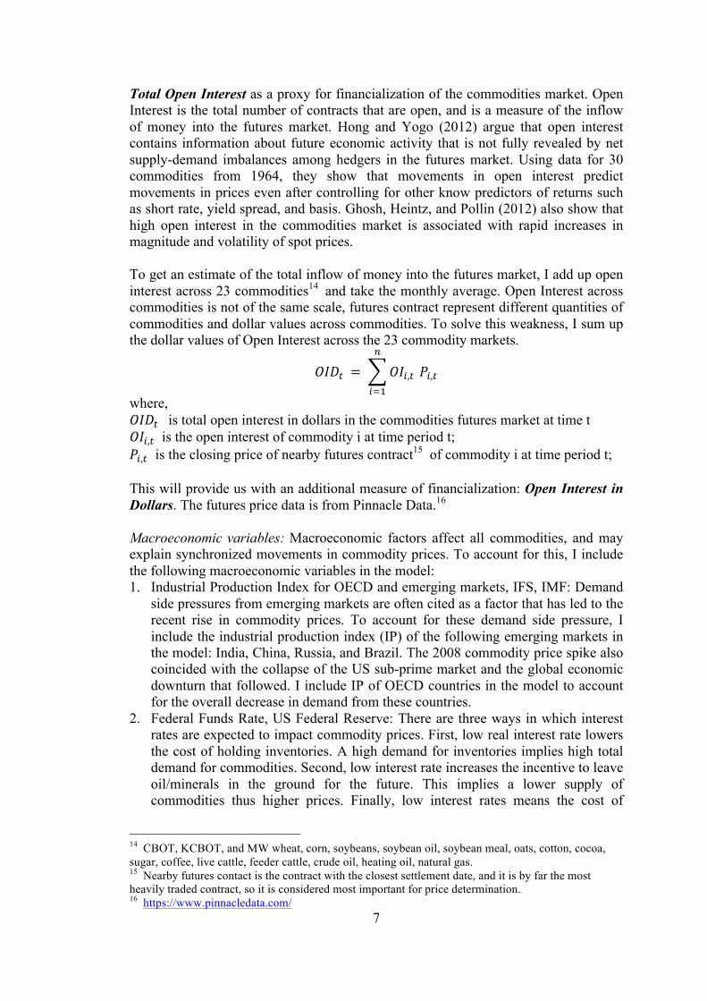
Total Open Interest as a proxy for financialization of the commodities market. Open Interest is the total number of contracts that are open, and is a measure of the inflow of money into the futures market. Hong and Yogo (2012) argue that open interest contains information about future economic activity that is not fully revealed by net supply-demand imbalances among hedgers in the futures market. Using data for 30 commodities from 1964, they show that movements in open interest predict movements in prices even after controlling for other know predictors of returns such as short rate, yield spread, and basis. Ghosh, Heintz, and Pollin (2012) also show that high open interest in the commodities market is associated with rapid increases in magnitude and volatility of spot prices. To get an estimate of the total inflow of money into the futures market, I add up open interest across 23 commodities14 and take the monthly average. Open Interest across commodities is not of the same scale, futures contract represent different quantities of commodities and dollar values across commodities. To solve this weakness, I sum up the dollar values of Open Interest across the 23 commodity markets.

𝑂𝐼𝐷!   =   𝑂𝐼!,!  

!

!!!

𝑃!,!

where, 𝑂𝐼𝐷!   is total open interest in dollars in the commodities futures market at time t 𝑂𝐼!,!     is the open interest of commodity i at time period t; 𝑃!,! is the closing price of nearby futures contract15 of commodity i at time period t; This will provide us with an additional measure of financialization: Open Interest in Dollars. The futures price data is from Pinnacle Data.16 Macroeconomic variables: Macroeconomic factors affect all commodities, and may explain synchronized movements in commodity prices. To account for this, I include the following macroeconomic variables in the model: 1. Industrial Production Index for OECD and emerging markets, IFS, IMF: Demand

side pressures from emerging markets are often cited as a factor that has led to the recent rise in commodity prices. To account for these demand side pressure, I include the industrial production index (IP) of the following emerging markets in the model: India, China, Russia, and Brazil. The 2008 commodity price spike also coincided with the collapse of the US sub-prime market and the global economic downturn that followed. I include IP of OECD countries in the model to account for the overall decrease in demand from these countries.

2. Federal Funds Rate, US Federal Reserve: There are three ways in which interest rates are expected to impact commodity prices. First, low real interest rate lowers the cost of holding inventories. A high demand for inventories implies high total demand for commodities. Second, low interest rate increases the incentive to leave oil/minerals in the ground for the future. This implies a lower supply of commodities thus higher prices. Finally, low interest rates means the cost of

14 CBOT, KCBOT, and MW wheat, corn, soybeans, soybean oil, soybean meal, oats, cotton, cocoa, sugar, coffee, live cattle, feeder cattle, crude oil, heating oil, natural gas. 15 Nearby futures contact is the contract with the closest settlement date, and it is by far the most heavily traded contract, so it is considered most important for price determination. 16 https://www.pinnacledata.com/

8

borrowing money is low and provides incentive for speculators to enter the commodities futures market. (Calvo 2008, Frankel 2006)

3. US Nominal Broad Exchange Rate, US Federal Reserve: Since a majority of commodities are traded in the international market in US dollars, if the USD depreciates, then the price of commodities in local currency will be lower, leading to higher demand (Akram 2008). I will use the US nominal broad exchange rate index which is a weighted average of the foreign exchange values of the USD against the currencies of a large group of major US trading partners.

4. US Inflation, urban, all items less food and energy, Bureau of Labor Statistics: Inflation can raise the overall level of commodity prices. To ensure that the measure of inflation is not contaminated by rise in prices of food and energy, I use the change in core CPI.

5. Crude Oil Price (WTI), International Financial Statistics, IMF: The link between energy and food prices, through transportation and fertilizer costs, is well established. Soaring oil prices have also increased interest in biofuels, which has further strengthened the link between food and fuel. Crude oil prices thus, can be considered an important macroeconomic determinant of commodity prices. However, crude oil prices themselves may be influenced by financialization. Therefore I carry-out the empirical analysis with and without crude oil prices in the model.

5. Empirical Results The first step in the empirical analysis is to provide evidence that in fact comovement between commodities has increased in recent years. A general rise over time in Pearson’s correlation coefficient among commodities is the simplest method to do so. Table A (appendix 2) shows correlation coefficient for select commodities (including grain, energy and soft commodities, livestock, and metals) for two time-periods 1995-2005 and 2006-2012. Except for a few cases, correlation is higher in the second time-period among most commodities. Even correlation between commodities that are seemingly unrelated such as copper and grains, have risen in the second-time period. Cluster analysis provides another method to analyze comovement among commodities. I use a single-linkage, agglomerative hierarchical clustering method. The dissimilarity measure or distance is defined as 1 minus the correlation coefficient. Commodities that have the smallest distance between them are first grouped into a cluster; finally after a number of steps, we end up with a single cluster containing all commodities. The result of cluster analysis can be shown by a dendrogram. In Figure A (appendix 2), the first dendrogram shows that gasoline and crude oil (WTI) have the smallest distance (or dissimilarity measure), so they are the first to be clustered together. In the next step, natural gas is added to the gasoline-crude oil cluster; while corn and sorghum is clustered together and so on. At the end of the process all the 41 commodities are grouped together. The second dendrogram is similarly constructed for the 2006-2012 time period. A comparison of the two dendrograms reveals that the dissimilarity measure between commodities has reduced substantially in the second period. Both the correlation matrix and cluster analysis reveal that comovement among commodities has increased in recent years. In the next step, I carry out unit root tests to understand stationarity properties of commodity prices. DFGLS and Dickey-Fuller unit root tests show all commodities are

9

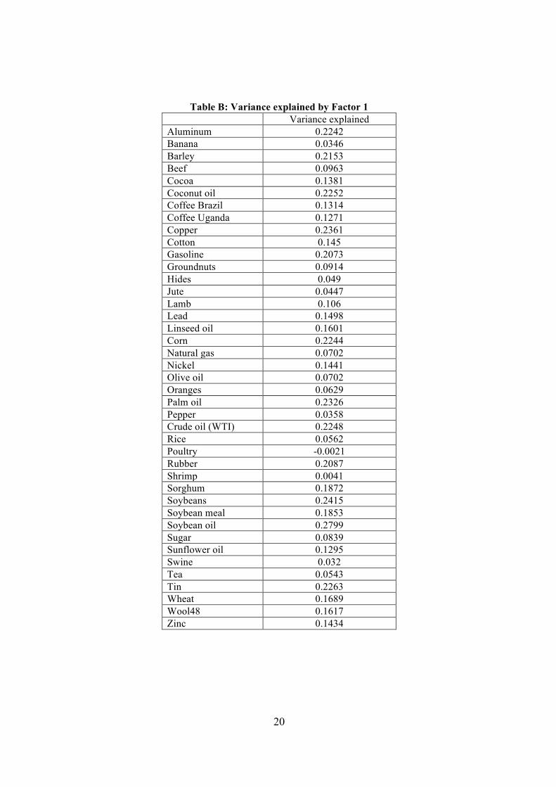
I(1). In the next step, I standardize (demean and divide by variance) 17 and first-difference the data and carry out the PANIC method on the set of 41 commodities. Table 1 below lists the extracted factors with eigenvalues > 1. The first factor is the most important as it explains 22 percent of the variance, the second factor explains about 6.7 percent of the variance and so on. Table B (Appendix 2) summarizes the share of variance explained by Factor 1 in each commodity. For soybean oil and copper factor 1 explains 28 and 23.64 percent of the variance respectively; while for rice it only explains 5 percent of the variance.

Table 1: Factors and Variance Explained Results of PCA Eigenvalues Cumulative variance

explained Variance explained

Factor 1 9.0521 0.2208 22.08 Factor 2 2.7390 0.2876 6.68 Factor 3 2.1819 0.3408 5.32 Factor 4 1.8119 0.385 4.42 Factor 5 1.6467 0.4252 4.02 Factor 6 1.4663 0.4609 3.57 Factor 7 1.4190 0.4955 3.46 Factor 8 1.3502 0.5285 3.30 Factor 9 1.2807 0.5597 3.12 Factor 10 1.2178 0.5894 2.97 Factor 11 1.1788 0.6182 2.88 Factor 12 1.0984 0.6449 2.67 Factor 13 1.0754 0.6712 2.63 Factor 14 1.0284 0.6963 2.51

As the extracted factor is in first-difference, I reconstruct Factor 1 in levels using the relationship f!!! = Δf!!! +   f! and assuming  f!  = 0. Figure 2 below graphs the reconstructed Factor 1 with Total Open Interest. Factor 1 appears to be moving in the opposite direction as Open Interest until early 2002; Factor 1 was declining while Open Interest was slowly increasing. Since 2002, the common factor and Open Interest have been moving in the same direction, with very strong correlation between 2008 and 2011.

17 As principal component analysis in not scale invariant, we need to standardize the data

10

Figure 2: Trends in Factor 1 and Total Open Interest

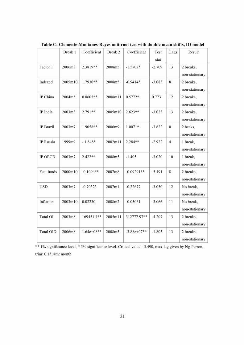
To understand the time series properties of the extracted Factor, I carry out unit root tests. I also perform unit root tests on the macroeconomic variables and the two proxies of financialization: Total Open Interest and Total Open Interest in Dollars. Results show that all the series are non-stationary (see Tables C and D in Appendix 2). Given all the variables are I(1), the next step in the analysis is to use a FAVEC model to examine if macroeconomic variables and proxies of financialization can explain developments in the extracted factor(s). To estimate the optimum lag length for the FAVEC model, I estimate a VAR model using maximum lag given by Ng-Perron criterion. For all models, Akaike Information Criterion (AIC), Hanna-Quin information criterion (HQIC), and Schwarz information criterion (SBIC) show 14, 2 and 1 lags respectively. I proceed with 2 lags and carry out Johansen’s cointegration test using both trace statistics and maximum eigenvalue test. Table E (Appendix 2) details the results. With Total Open Interest as proxy for financialization, trace test shows that we cannot reject the null hypothesis that rank ≤ 2; while eigenvalue test shows that we cannot reject the null hypothesis that rank = 2. As results from both tests are consistent, I proceed with rank = 2. Results are similarly consistent using Total Open Interest in Dollars as a proxy (rank=2). The VEC model assumes that the residuals approximate white noise. I examine this assumption by performing Lagrange Multiplier (LM) test for serial correlation and Jarque-Bera normality tests. Unfortunately, with the 2 lags model, residuals show evidence of serial correlation and excess skewness and kurtosis. I repeat the exercise with 14 lags (given by AIC) and in this case residuals are not serially correlated. Table F (Appendix 2) summarizes the results for the normality tests with 14 lags model. The residuals are skewed for 3 variables in each model: US exchange rage, IP of OECD and Russia for the first model, and exchange rate, IP of India and Russia for the second model. The residuals are kurtotic for exchange rate and IP of Russia for both models. Skewness is considered a more important assumption than kurtosis for normality of residuals.18 Given these results I proceed with the rest of the empirical

18 Normality test is more sensitive to deviations from normality due to skewness than kurtosis because

11

analysis using 14 lags. I carry out four models with the two proxies for financialization, with and without crude oil prices. The first cointegrating equation in each model establishes the relationship between Factor 1 and proxies of financialization, Total Open Interest or Total Open Interest in Dollars. The proxies of financialization are significant and have the expected negative sign in all four models. IP of OECD is not significant in M2 and M3; while IP of China is not significant for M3. Federal funds rate is not significant in any of the models, while IP of Russia is only significant in M2. The US dollar is significant in all models except M4. In M3, only three variables are significant: the US dollar, crude oil prices and the proxy for financialization. Table G (Appendix 2) summarizes the results. I restrict the coefficients of insignificant variables to be 0 and re-estimate the model.19 Table 1 summarizes the results of restricted FAVEC models. Both proxies of financialization, Total Open Interest and Total Open Interest in Dollars are significant in all four models. They also have the expected negative sign, implying that Open Interest and Factor 1 move in the same direction; as Open Interest increases, comovement between commodity prices increases. IP of India is significant in M1 and M2, but has a positive sign; IP of China is significant for M1, M2 and M4, and has the expected negative sign for M1 and M2. IP of Brazil is significant with the expected sign for M1, M2 and M3, while IP of Russia is not significant in any of the models. These results imply that demand from China and Brazil may have been a factor in causing the rise in commodity prices. Crude oil is only significant in M1 and M3, and has the expected negative sign only in M3. The USD exchange rate is significant in M1, M2 and M3, and has the expected positive sign. This implies that appreciation of the USD leads to a decrease in demand for commodities (due to rise in prices in local currency) and hence a drop in international prices across commodities. Overall, these results provide strong evidence to support the thesis that the rise in liquidity in the commodities futures market led to the increase in comovement of commodity prices.

Table 1: Restricted VECM Results for Factor 1

M1 M2 M3 M4 exchange rate 1.31*** 1.21*** 0.96*** --

IP OECD -0.57*** -- -- 2.24*** IP India 1.94*** 1.11*** -- -- IP China -1.50*** -0.94*** -- 1.35*** IP Brazil -1.83*** -1.79*** -- -1.79*** IP Russia -- 0.12 -- -- Crude oil 0.73*** -- -0.19*** -- Total OI -0.09*** -0.03** -- --

Total OID -- -- -0.0001*** -0.0003*** constant -22.44 -31.80 -9.10 -43.32

Factor 1 = 1. *** 1% significance, ** 5% significance, * 10% significance

the variance of skewness is smaller than the variance of kurtosis (Juselius 2006, p.75). 19 Chi-square tests reveal that these restrictions are not rejected.

12

6. Conclusion In this paper, I explored one of the distinctive features of the 2008 commodity price developments -- the remarkably synchronized rise and fall of prices of unrelated commodities. Unlike related commodities, that are either complements or substitutes in production or consumption, comovement of prices of unrelated commodities cannot be explained by commodity specific demand and supply shocks. Only factors that affect several commodity markets simultaneously can explain such comovement. Financialization of the commodities futures market refers to the massive inflow of investment in the market, and the rise of commodities as an investment asset. Financialization may cause co-movement between commodity prices through three mechanisms: i) commodity futures are bought and sold together not based on fundamentals, but based on pre-set weights of commodity indices; ii) due to liquidity effects of commodity speculators trade in two or more commodity markets; and iii) due to transmission of shocks in energy markets to other commodities due to the higher weight of energy commodities in popular commodity indices. In this paper, I explored if financialization of the commodities futures market can explain the recent rise in commodity price comovement. For the empirical analysis, I extracted common factors from the entire set of 41 commodities using the PANIC method of Bai and Ng (2004). Factor 1 that explains 22 percent of the variance in prices was extracted and saved for further analysis. Factor 1 was moving in the opposite direction Total Open Interest until 2002, however since then they have been moving in the same direction, with very strong correlation during 2008-11. The extracted factor was then included in a FAVEC model along with other macroeconomic factors including: industrial production indices of OECD and major emerging countries, inflation, USD exchange rate, and crude oil prices. Instead of assuming the excess comovement that is unexplained by macroeconomic factors is due to speculation, I add proxies of financialization in the FAVEC model. This is a stronger and more direct evidence of the role of financialization in explaining comovement of commodity prices than previously provided in the literature. The empirical analysis shows that both proxies of financialization, Total Open Interest and Total Open Interest in Dollars, are significant and have the expected negative sign in all four models. These results imply that as financialization of the commodities futures market proceeded and more traders entered the futures market, market liquidity increased. Much of the rise in liquidity was due to increasing investment in commodity indices, which meant that futures of unrelated commodities were being bought and sold together as part of a portfolio. This increase in liquidity across different commodity markets, lead to the synchronized rise (and fall) in commodity prices. Overall, this paper provides strong empirical evidence that financialization of the commodities market led to the recent rise in comovement of (unrelated) commodity prices.

13

References Ai, C., Chatrath, A., & Song, F. 2006. On the Comovement of Commodity Prices. American Journal of Agricultural Economics, 88(3), 574-588. Akram, Q. F. 2008. Commodity Prices, Interest Rates, and the Dollar. Norges Bank Working Paper 2008/12, August. Bai, J. & Ng, S. 2004. A PANIC Attach on Unit Roots and Cointegration” Econometrica, 72(4), 1127-1177. Banerjee, A. & Marcellino, M. 2008. Factor-augmented Error Correction Models. IGIER Working Paper 335, February. Bernanke, B. S., Boivin, J., & Eliasz, P. 2005. Measuring the Effects of Monetary Policy: A Factor-Augmented Vector Autoregressive (FAVAR) Approach. Quarterly Journal of Economics, 120(1), 387-422. Buyuksahin, B., Haigh, M., & Robe, M. 2010. Commodities and equities: Ever a “Market of One”? Journal of Alternative Investments, 12(3), 76-95. Buyuksahin, B. & Robe, M. 2011. Does “Paper Oil” Matter? Energy Markets’ Financialization and Equity-Commodity Co-Movements. July. Retrieved from: http://www.parisschoolofeconomics.eu/IMG/pdf/buyuksahin_paper.pdf Byrne, J. P., Fazio, G., & Fiess, N. 2011. Primary Commodity Prices: Co-movements Common Factors and Fundamentals. Policy Research Working Paper 5578, World Bank. Calvo, G. 2008. Exploding Commodity Prices, Lax Monetary Policy, and Sovereign Wealth Funds. Retrieved from: http://www.voxeu.org/index.php?q=node/1244 Cashin, P., McDermott, J. C., & Scott, A. 1999. The Myth of Comoving Commodity Prices. International Monetary Fund Working Paper WP/99/169. Chong, J. & Miffre, J. 2008. Conditional Return Correlations between Commodity Futures and Traditional Assets. EDHEC Risk and Asset Management Research Centre, April. Cuddington, J. T. & Jerrett, D. 2008. Super Cycles in Real Metals Prices? IMF Staff Papers, 55(4). International Monetary Fund. Deb, P., Trivedi, P., & Varangis, P. 1996. The Excess Co-movement of Commodity Prices Reconsidered. Journal of Applied Econometrics, 11(3), 275-91. Erb, C. & Harvey, C. 2006. The Strategic and Tactical Value of Commodity Futures. Financial Analysts Journal, 62(2), 69-97. Francis, N., Owyang, M. T., & Savascin, O. 2011. An Endogenous Clustered Factor

14

Approach to International Business Cycles. Department of Economics, University of North Carolina, Chapel Hill, January. Frankel, J. & Rose, A. 2009. Determinants of Agricultural and Mineral Commodity Prices. Working Paper, Kennedy School of Government, Harvard University. Epstein, G. and Jayadev, A. 2005. “The Rise of Rentier Incomes in OECD Countries: Financialization, Central Bank Policy, and Labor Solidarity” in Gerald Epstein ed., Financialization and the World Economy, 46-76. Ghosh, J. 2010. The Unnatural Coupling: Food and Global Finance. Journal of Agrarian Change 10(1), 72-86. Ghosh, J., Heintz, J. & Pollin, R. 2012. Speculation of Commodities Futures Markets and Destablization of Global Food Prices: Exploring the Connections. International Journal of Health Services, 42(3), 465-483. Gilbert, C. L 2010. How to Understand High Food Prices. Journal of Agricultural Economics 61, 398-425. Gorton, G. & Rouwenhorst, K. G. 2004. Facts and Fantasies about Commodity Futures. Yale ICF Working Paper 4-20, June. Greer, R. 2000. The Nature of Commodity Index Returns. Journal of Alternative Investments, Summer. Hamilton, J. D. 2009. Causes and Consequences of the Oil Shock of 2007-08. Brookings Papers on Economic Activity, Spring 1, 215-259. Hong, H. & Yogo, M. 2012. What Does Futures Market Interest Tell Us about The Macroeconomy and Asset Prices. Journal of Financial Economics, Elsevier, 105(3), 473-490. Krugman, P. 2008. Speculative Nonsense Once Again. Retrieved from: http://krugman.blogs.nytimes.com/2008/06/23/speculative-nonsense-once-again/ Lescaroux, F. 2009. On the Excess Comovement of Commodity Prices- A Note about the Role of Fundamental Factors in Short-run Dynamics. Energy Policy, 37 (10), 3906-3913. Lombardi, M., Osbat, C. & Schnatz, B. 2010. Global Commodity Cycles and Linkages: A FAVAR Approach. Working Paper Series 1170, European Central Bank, April. Mayer, J. 2009. The Growing Interdependence Between Financial and Commodity Markets. UNCTAD Discussion Paper 195. Orhangazi, O. (2008). Financialisation and Capital Accumulation in the Non-financial Corporate Sector: A Theoretical and Empirical Investigation on the US Economy: 1973-2003. Cambridge Journal of Economics, 32, 863-886.

15

Palaskas, T. B. & Varangis, P. N. 1991. Is There Excess Co-Movement of Primary Commodity Prices? A Co-integration Test. WPS 758, World Bank, August. Pindyck, R. & Rotemberg, J. 1990. The Excess Co-movement of Commodity Prices. Economic Journal, 100 (403), 1173-1189. Pollin, R., and Heintz, J. 2012. Study of U.S. Financial System, FESSUD Studies in Financial Systems No. 10. FESSUD studies in Financial Systems. http://fessud.eu/?page_id=665 Robles, M., Torero, M., & Braun, J. V. 2009. When Speculation Matters. IFPRI Policy Brief 57. International Food Policy Research Institute. Washington DC. Savascin, O. 2011. The Dynamics of Commodity Prices: A Clustering Approach. Department of Economics, University of North Carolina, Chapel Hill, November. Silvennoinen, A. & Thorp, S. 2010. Financialization, Crisis and Commodity Correlation Dynamics. Working Paper, Queensland University of Technology. Tang, K. & Xiong, W. 2010. Index Investment and Financialization of Commodities. Princeton University Working Paper 16385, September. UNCTAD. 2009. Trade and Development Report. UNCTAD. USDA. 2009. Food Security Assessment 2008-09. United States Department of Agriculture, June. Vansteenkiste, I. 2009. How Important are Common Factors in Driving Non-Fuel Commodity Prices? A Dynamic Factor Analysis. European Central Bank Working Paper Series 1072, July.

16

Appendix 1: Data Details and Sources Commodity Prices, International Financial Statistics, IMF, Monthly Description taken from the IFS database

1. Aluminum: LME, standard grade, spot price, 99.5% minimum purity, CIF UK ports, US$ per metric ton.

2. Bananas: Central America and Ecuador, first class quality tropical pack, US importer’s price FOB U.S. Ports, US$ per metric ton.

3. Barley: Canada, no.1 Western Barley, spot price, Winnipeg Commodity Exchange, US$ per metric ton.

4. Beef: Australia and New Zealand, frozen boneless, 85% visible lean cow meat, US import price FOB US port of entry, US cents per pound.

5. Cocoa Beans: New York and London, International Cocoa Organization daily price, Average of the daily prices of the nearest three active future trading months. CIF US and European ports, US$ per metric ton.

6. Coconut Oil: Philippines/Indonesia, US $ per metric ton. 7. Coffee (Brazil): Unwashed Arabica, Santos No. 4, ex-dock, New York 8 Coffee (Uganda): Robusta, New York Cash Price, Cote d’Ivoire Grade II, and

Uganda Standard. Prompt shipment, ex-dock, New York 9. Copper: United Kingdom, grade A cathode, LME spot price, CIF European ports,

US$ per metric ton. 10 Corn (Maize): United States. No.2 Yellow, FOB Gulf of Mexico, US$ per metric

ton. 11. Cotton: Cotton Outlook, Liverpool Index A, Middling 1-3/32 inch staple, CIF

Liverpool, US cents per pound. 12. Crude Oil WTI: United States, West Texas Intermediate (WTI), 40 API, spot, FOB

midland Texas, US$ per barrel. 13. Gasoline: regular unleaded, Petroleum Product Assessments, US cents per gallon 14. Groundnuts: Any origin, 40 to 50 count per ounce, in-shell Argentina, US $ per ton. 15. Hides: United States, Heavy native steers, over 53 pounds, wholesale dealer’s price,

Chicago, fob Shipping Point, US cents per pound. 16. Jute: Raw Bangladesh, FOB Chittagong/Chalna, US $ per ton. 17. Lamb: New Zealand, frozen, wholesale price at Smithfield Market London. US cents

per pound. 18. Lead: United Kingdom, 99.97% pure, LME spot price, CIF European Ports, US$ per

metric ton. 19. Linseed Oil: Any Origin, ex-tank Rotterdam, US $ per ton. 20. Natural Gas: United States, Natural Gas Spot Price, Henry Hub, Louisiana, US$ per

Thousands of Cubic Meters. 21. Nickel: United Kingdom, LME melting grade, spot, CIF North European Ports,

US$ per ton.  22. Olive Oil: United Kingdom, extra virgin less than 1% free fatty acid, ex-tanker price

U.K., US$ per metric ton.  23. Oranges: France, miscellaneous oranges CIF French import price, US$ per metric

ton.  24. Palm oil: Malaysia, Crude Palm Oil Futures (first contract forward) 4-5 percent FFA,

US$ per metric ton  25. Pepper: Malaysia, Black, average US wholesale price, bagged, carlots, FOB New

York. US cents per pound.  26. Poultry (chicken): United States, Whole bird spot price, Ready-to-cook, whole, iced,

Georgia docks, US cents per pound. 27. Rice: Thailand, 5 percent broken milled white rice, Thailand nominal price quote,

FOB Bangkok, US$ per ton.  

17

28. Rubber: Malaysia, No.1 Smoked Sheet, FOB Malaysia/Singapore ports, US cents per pound  

29. Shrimp: United States, No.1 shell-on headless, 26-30 count per pound, Mexican, New York port, US cents per pound.  

30. Sorghum: United States, No 2 Yellow, FOB Gulf of Mexico ports, US $ per ton.  31. Soybeans: United States, Chicago Soybean futures contract (first contract forward)

No. 2 yellow and par, US$ per metric ton. 32. Soybean Meal: United States, Chicago Soybean Meal Futures (first contract forward)

Minimum 48 percent protein, US$ per metric ton.  33. Soybean Oil: United States, Chicago Soybean Oil Futures (first contract forward)

exchange approved grades, US$ per metric ton.  34. Sugar: United States import price, contract no.14 nearest futures position, US cents

per pound.  35. Sunflower oil: United Kingdom, US export price from Gulf of Mexico, US$ per

metric ton.  36. Swine Meat (pork): United States (Iowa), 51-52% lean hogs, US cents per pound.  37. Tea: Mombasa, Kenya, Auction Price for best PF1, Kenyan tea. US cents per

kilogram.  38. Tin: Any origin, United Kingdom LME spot price, standard grade, spot, CIF

European ports. US$ per metric ton.  39. Wheat: United States, No.1 Hard Red Winter, ordinary protein, FOB Gulf of Mexico,

US$ per metric ton 40. Wool 48’s: Austraila-New Zealand, coarse wool 23 micron, Australian Wool

Exchange spot quote, US cents per kilogram. 41. Zinc: United Kingdom, LME, high grade 98% pure, spot, CIF UK ports, US$ per

metric ton.

18

Appendix 2: Results Figure A: Dendrograms

0.2

.4.6

.8

Dis

sim

ilarit

y m

easu

re

alum

iniu

mco

pper

lead

rubb

erol

ive

oil

tinbe

efga

solin

ecr

ude

oil

natu

ral g

asni

ckel

iron

ore

sunf

low

er o

illin

seed

oil

barle

yco

rnso

rghu

mw

heat

oran

ges

poul

tryco

conu

t oil

coffe

e B

razi

lco

ffee

Uga

nda

cotto

nric

epa

lm o

ilso

ybea

n oi

lso

ybea

nsso

ybea

n m

eal

swin

ezi

ncco

coa

woo

l48

lam

bju

tesu

gar

pepp

ersh

rimp

tea

grou

ndnu

tshi

des

bana

nas

Dendrogram of Commodities 1995-20050

.2.4

.6.8

Dis

sim

ilarit

y m

easu

re

alum

iniu

mni

ckel

zinc

lam

bna

tura

l gas

oliv

e oi

lsh

rimp

bana

nas

barle

ygr

ound

nuts

corn

sorg

hum

coffe

e U

gand

apa

lm o

ilso

ybea

n oi

lso

ybea

nsso

ybea

n m

eal

linse

ed o

ilco

conu

t oil tin

cotto

nru

bber

beef

pepp

erw

ool4

8co

ffee

Bra

zil

iron

ore

suga

rpo

ultry

whe

atga

solin

ecr

ude

oil

coco

aju

te tea

swin

eco

pper

rice

sunf

low

er o

ilhi

des

lead

oran

ges

Dendrogram of Commodities 2006-2012

19

Table A: Correlation Matrix

Pearson’s correlation coefficient: first row 1995-2005, second row 2006-2012 Source: author’s own calculations

20

Table B: Variance explained by Factor 1 Variance explained

Aluminum 0.2242 Banana 0.0346 Barley 0.2153 Beef 0.0963 Cocoa 0.1381 Coconut oil 0.2252 Coffee Brazil 0.1314 Coffee Uganda 0.1271 Copper 0.2361 Cotton 0.145 Gasoline 0.2073 Groundnuts 0.0914 Hides 0.049 Jute 0.0447 Lamb 0.106 Lead 0.1498 Linseed oil 0.1601 Corn 0.2244 Natural gas 0.0702 Nickel 0.1441 Olive oil 0.0702 Oranges 0.0629 Palm oil 0.2326 Pepper 0.0358 Crude oil (WTI) 0.2248 Rice 0.0562 Poultry -0.0021 Rubber 0.2087 Shrimp 0.0041 Sorghum 0.1872 Soybeans 0.2415 Soybean meal 0.1853 Soybean oil 0.2799 Sugar 0.0839 Sunflower oil 0.1295 Swine 0.032 Tea 0.0543 Tin 0.2263 Wheat 0.1689 Wool48 0.1617 Zinc 0.1434

21

Table C: Clemente-Montanes-Reyes unit-root test with double mean shifts, IO model

Break 1 Coefficient Break 2 Coefficient Test

stat

Lags Result

Factor 1 2006m8 2.3819** 2008m5 -1.5707* -2.709 13 2 breaks,

non-stationary

Indexed 2005m10 1.7930** 2008m5 -0.9414* -3.083 8 2 breaks,

non-stationary

IP China 2004m5 0.8605** 2008m11 0.5772* 0.773 12 2 breaks,

non-stationary

IP India 2003m3 2.791** 2005m10 2.623** -3.023 13 2 breaks,

non-stationary

IP Brazil 2003m7 1.9058** 2006m9 1.0071* -3.622 0 2 beaks,

non-stationary

IP Russia 1999m9 - 1.848* 2002m11 2.284** -2.922 4 1 break,

non-stationary

IP OECD 2003m7 2.422** 2008m5 -1.405 -3.020 10 1 break,

non-stationary

Fed. funds 2000m10 -0.1094** 2007m8 -0.09291** -5.491 8 2 breaks,

non-stationary

USD 2003m7 -0.70323 2007m1 -0.22677 -3.050 12 No break,

non-stationary

Inflation 2003m10 0.02230 2008m2 -0.05061 -3.066 11 No break,

non-stationary

Total OI 2003m8 169451.4** 2005m11 312777.97** -4.207 13 2 breaks,

non-stationary

Total OID 2006m8 1.64e+08** 2008m5 -3.88e+07** -1.803 13 2 breaks,

non-stationary

** 1% significance level, * 5% significance level. Critical value: -5.490, max-lag given by Ng-Perron,

trim: 0.15, #m: month

22

Table D: DFGLS and Dickey Fuller Unit root tests for extracted factors

Lags DFGLS

test

Dfuller w/

constant

Dfuller no

constant

Dfuller

w/ trend

Result

Factor 1 (level) 13 -1.292 -1.656 -1.079 -2.418 I(1)

Factor 1 (diff.) 12 -4.845** -4.102** -4.115** -4.279*

Indexed (level) 13 -1.31078 -1.5209 -1.12074 -2.433 I(1)

Indexed (diff.) 12 -4.50525 -4.5677** -4.58114 -4.669**

IP OECD (level) 14 -3.038* 0.533 -2.563 -3.026 I(1)

IP OECD (diff.) 14 -1.521 -5.495** -5.618** -5.822**

IP China (level) 14 -1.469 -0.542 -1.958 -2.216 I(1)

IP China (diff.) 14 -2.535 -4.830** -4.819** -4.806**

IP India (level) 13 -1.092 2.363* 1.103 -1.762 I(1)

IP India (diff.) 12 -1.072 -1.880 -3.083* -3.687*

IP Brazil (level) 14 -1.724 -1.920 -0.508 -2.950 I(1)

IP Brazil (diff.) 14 -3.055* -4.295** -4.796** -4.782**

IP Russia (level) 12 -1.725 -0.041 -1.814 -2.451 Non-stationary

IP Russia (diff.) 11 -1.770 -2.770** -2.771 -2.949

Inflation (level) 13 -2.489 -0.500 -2.761 -2.726 I(1)

Inflation (diff.) 14 -1.543 -6.103** -6.086** -6.079**

Nom. exchange rate (level) 2 -0.637 -0.122 -1.661 -2.247 I(1)

Nom. exchange rate (diff.) 9 -2.161 3.940** -3.926** -4.356**

Total OI (level) 13 -1.66109 -0.56631 1.003016 -2.13189 I(1)

Total OI (diff.) 12 -2.8812* -3.8247** -3.5193** -3.8152*

Total OID (level) 13 -1.6157 -0.20705 0.734472 -2.30445 I(1)

Total OID (diff.) 12 -3.6932** -4.7596** -4.6157** -4.879**

Fed funds rate (level) 9 -3.097* -1.465 -1.902 -3.177 I(1)

Fed funds rate (diff.) 14 -3.389* -3.401** -3.495** -3.489*

23

Table E: Johansen’s Cointegration Test: Trace and Max Eigenvalue Tests

Total OI Total OID

Rank Trace stat Max test Trace stat Max test

0 398.13 185.89 406.19 189.78

1 212.243 59.491 216.41 57.46

2 152.7** 43.9** 158.9** 48.13**

Table F: Normality Tests of the Residuals from VECM with 14 lags

Skewness Kurtosis Skewness Kurtosis

All 41 Indexed All 41 Indexed All 41 Indexed All 41 Indexed

Factor 1 -0.024

(0.891)

-0.228

(0.188)

2.830

(0.623)

2.748

(0.466)

-0.072

(0.679)

-0.234

(0.177)

2.879

(0.728)

3.458

(0.186)

inflation -0.076

(0.662)

-0.168

(0.331)

3.011

(0.976)

2.782

(0.529)

-0.171

(0.322)

-0.353

(0.042)

2.807

(0.577)

2.868

(0.703)

USD -0.542

(0.002)

-0.457

(0.008)

4.167

(0.001)

4.343

(0.000)

-0.495

(0.004)

-0.323

(0.062)

4.433

(0.000)

4.258

(0.000)

IP OECD -0.459

(0.008)

-0.311

(0.073)

3.530

(0.126)

3.226

(0.514)

-0.339

(0.051)

-0.458

(0.008)

3.552

(0.111)

3.544

(0.116)

IP India 0.048

(0.780)

0.093

(0.593)

3.228

(0.510)

3.098

(0.777)

0.492

(0.005)

0.226

(0.192)

3.364

(0.293)

3.239

(0.491)

IP China -0.273

(0.115)

-0.284

(0.101)

3.201

(0.562)

3.494

(0.154)

-0.042

(0.810)

-0.386

(0.026)

3.156

(0.652)

3.848

(0.014)

IP Brazil 0.070

(0.684)

0.088

(0.611)

2.949

(0.883)

3.275

(0.427)

0.048

(0.783)

-0.041

(0.812)

3.044

(0.899)

3.321

(0.354)

IP Russia 0.539

(0.002)

0.874

(0.000)

6.988

(0.000)

9.374

(0.000)

0.591

(0.001)

1.080

(0.000)

6.140

(0.000)

11.226

(0.000)

Crude oil 0.030

(0.862)

-0.071

(0.682)

2.841

(0.647)

3.058

(0.866)

0.011

(0.947)

0.235

(0.174)

3.125

(0.718)

3.603

(0.082)

Total OI -0.157

(0.365)

-0.308

(0.075)

3.419

(0.227)

3.259

(0.455) -- -- -- --

Total OID -- -- -- -- -0.100

(0.562)

-0.187

(0.280)

3.012

(0.972)

3.246

(0.477)