NBER WORKING PAPER SERIES

FINANCIAL INNOVATION AND THE TRANSACTIONS DEMAND FOR CASH

Fernando E. AlvarezFrancesco Lippi

Working Paper 13416http://www.nber.org/papers/w13416

NATIONAL BUREAU OF ECONOMIC RESEARCH1050 Massachusetts Avenue

Cambridge, MA 02138August 2007

We thank Daron Acemoglu for constructive criticisms on a previous version of the paper. We alsothank Alessandro Secchi for his guidance in the construction and analysis of the database. We benefitedfrom the comments of Manuel Arellano, V.V. Chari, Luigi Guiso, Bob Lucas, Greg Mankiw, FabianoSchivardi, Rob Shimer, Pedro Teles, Randy Wrigth and seminar participants at the University of Chicago, University of Sassari, Harvard University, MIT, Wharton School, Northwestern, FRB of Chicago,FRB of Minneapolis, Bank of Portugal, European Central Bank, Bank of Italy, CEMFI, EIEF, Universityof Cagliari, University of Salerno, Austrian National Bank, Tilburg University and Erasmus UniversityRotterdam. The views expressed herein are those of the author(s) and do not necessarily reflect theviews of the National Bureau of Economic Research.

© 2007 by Fernando E. Alvarez and Francesco Lippi. All rights reserved. Short sections of text, notto exceed two paragraphs, may be quoted without explicit permission provided that full credit, including© notice, is given to the source.

Financial Innovation and the Transactions Demand for CashFernando E. Alvarez and Francesco LippiNBER Working Paper No. 13416August 2007, Revised May 2008JEL No. E31,E4,E41

ABSTRACT

We document cash management patterns for households that are at odds with the predictions of deterministicinventory models that abstract from precautionary motives. We extend the Baumol-Tobin cash inventorymodel to a dynamic environment that allows for the possibility of withdrawing cash at random timesat a low cost. This modification introduces a precautionary motive for holding cash and naturallycaptures developments in withdrawal technology, such as the increasing diffusion of bank branchesand ATM terminals. We characterize the solution of the model and show that qualitatively it is ableto reproduce the empirical patterns. Estimating the structural parameters we show that the modelquantitatively accounts for key features of the data. The estimates are used to quantify the expenditureand interest rate elasticity of money demand, the impact of financial innovation on money demand,the welfare cost of inflation, the gains of disinflation and the benefit of ATM ownership.

Fernando E. AlvarezUniversity of ChicagoDepartment of Economics1126 East 59th StreetChicago, IL 60637and NBERf-alvarez1@uchicago.edu

Francesco LippiUniversity of SassariDepartment of EconomicsandEnte Einaudi,via Due Macelli, 7300184 Rome - Italyflippi@uniss.it

1 Introduction

There is a large literature arguing that financial innovation is important for under-

standing money demand, yet seldom this literature integrates the empirical analysis

with an explicit modeling of the financial innovation. In this paper we develop a dy-

namic inventory model of money demand that explicitly incorporates the effects of

financial innovation on cash management. We estimate the structural parameters of

the model using detailed micro data from Italian households, and use the estimates

to revisit several classic questions on money demand.

As standard in the inventory theory we assume that non-negative cash holdings

are needed to pay for consumption purchases. We extend the Baumol-Tobin model

to a dynamic environment which allows for the opportunity of withdrawing cash at

random times at low or zero cost. Cash withdrawals at any other time involve a

fixed cost, b. In particular, the expected number of such opportunities per period

of time is described by a single parameter, p. Examples of such opportunities are

finding an ATM that does not charge a fee, or passing by a bank desk at a time

with a low opportunity cost. Another interpretation of p is that it measures the

probability that an ATM terminal is working properly or a bank desk is open for

business. Financial innovations, such as the increase in the number bank branches

and ATM terminals, can be modeled by increases in p and decreases in b.

Our model changes the predictions of the Baumol-Tobin model (BT henceforth)

in ways that are consistent with stylized facts concerning households’ cash man-

agement behavior. The randomness introduced by p gives rise to a precautionary

motive for holding cash: when agents have an opportunity to withdraw cash at

zero cost they do so even if they have some cash at hand. Thus, the average cash

balances held at the time of a withdrawal relative to the average cash holdings,

M/M , is a measure of the strength of the precautionary motive. This ratio ranges

between zero and one and is increasing in p. Using household data for Italy and the

US we document that M/M is about 0.4, instead of being zero as predicted by the

BT model. Another property of our model is that the number of withdrawals, n,

increases with p, and the average withdrawal size W decreases, with W/M ranging

between zero and two. Using data from Italian households we measure values of n

and W/M that are inconsistent with those predicted by the BT model.

The model studies how to finance a constant flow of cash expenditures, the value

of which is taken as given both in the theory and in the empirical implementa-

tion. Hence the model abstracts from the cash/credit choice i.e. from the choice of

1

whether to have a credit card, and for those that have a credit card, of whether a

particular purchase is done using cash or credit. Formally, we are assuming separa-

bility between cash vs. credit purchases. We are able to study this problem for the

Italian households because we have a measure of the consumption purchases done

with cash. We view our paper as an input on the study of the cash/credit decision,

an important topic that we plan to address in the future.

We organize the analysis as follows. In Section 2 we use a panel data of Italian

households to illustrate key cash management patterns, including the strength of

precautionary motive, to compare them to the predictions of the BT model, and

motivate the analysis that follows.

Sections 3 and 4 present the theory. Section 3 analyzes the effect of financial

diffusion using a version of the BT model where agents have a deterministic number

of free withdrawals per period. This model provides a simple illustration of how

technology affects the level and the shape of the money demand (i.e. its interest

and expenditure elasticities). Section 4 introduces our benchmark stochastic dy-

namic inventory model. In this model agents have random meetings with a financial

intermediary in which they can withdraw money at no cost, a stochastic version of

the model of Section 3. We solve analytically for the Bellman equation and char-

acterize its optimal decision rule. We derive the distribution of currency holdings,

the aggregate money demand, the average number of withdrawals, the average size

of withdrawals, and the average cash balances at the time of a withdrawal. We

show that a single index of technology, b · p2, determines both the shape of the

money demand and the strength its precautionary component. While technological

improvements (higher p and lower b) unambiguously decrease the level of money

demand, their effect on this index −and hence on the shape and the precaution-

ary component of money demand− is ambiguous. The structural estimation of the

model parameters will allow us to shed light on this issue. We conclude the section

with the analysis of the welfare implications of our model and a comparison with

the standard analysis as reviewed in Lucas (2000).

Sections 5, 6 and 7 contain the empirical analysis. In Section 5 we estimate the

model using the panel data for Italian households. The two parameters p and b are

overidentified because we observe four dimensions of household behavior: M , W ,

M and n. We argue that the model has a satisfactory statistical fit and that the

patterns of the estimates are reasonable. For instance, we find that the parameters

for the households with an ATM card indicate their access to a better technology

(higher p and lower b). The estimates also indicate that technology is better in

2

locations with higher density of ATM terminals and bank branches. Section 6 stud-

ies the implications of our findings for the time pattern of technology and for the

expenditure and interest elasticity of the demand for currency. The estimated pa-

rameters reproduce the sizeable precautionary holdings present in the data. Even

though our model can generate interest rate elasticities between zero and 1/2, and

expenditure elasticities between 1/2 and one, the values implied by our estimates

are close to 1/2 for both, the values of the BT model. We discuss how to reconcile

our estimates of the interest rate elasticity with the smaller values typically found

in the literature.1 In Section 7 we use the estimates to quantify the welfare cost of

inflation −in particular the gains from the Italian disinflation in the 1990s− and the

benefits of ATM card ownership.

2 Cash Holdings Patterns of Italian Households

Table 1 presents some statistics on the cash holdings patterns by Italian households

based on the Survey of Household Income and Wealth.2 For each year we report

cross section means of statistics where the unit of analysis is the household. We

report statistics separately for households with and without ATM cards. All these

households have checking accounts that pay interests at rates documented below.

The survey records the household expenditure paid in cash during the year (we

use cash and currency interchangeably to denote the value of coins and banknotes).

The table displays these expenditures as a fraction of total consumption expenditure.

The fraction paid with cash is smaller for households with an ATM card, it displays

a downward trend for both type of households, though its value remains sizeable

as of 2004. These percentages are comparable to those for the US between 1984

and 1995.3 The table reports the sample mean of the ratio M/c, where M is the

1We remark that our interest rate elasticity, as in the BT model, refers to the ratio of moneystock to cash consumption. Of course if cash consumption relative to total consumption is afunction of interest rates, as in the Stokey-Lucas cash credit model, the elasticity of money tototal consumption will be even higher. A similar argument applies to the expenditure elasticity.The distinction is important to compare our results with estimates in the literature, that typicallyuse money/total consumption. See for instance Lucas (2000), who uses aggregate US data, orAttanasio, Guiso and Jappelli (2002), who use the same household data used here.

2This is a periodic survey of the Bank of Italy that collects data on several social and economiccharacteristics. The cash management information that we are interested in is only available since1993.

3Humphrey (2004) estimates that the mean share of total expenditures paid with currency inthe US is 36% and 28% in 1984 and 1995, respectively. If expenditures paid with checks areadded to those paid with currency, the resulting statistics is about 85% and 75% in 1984 and1995, respectively. The measure including checks is used by Cooley and Hansen (1991) to compute

3

average currency held by the household during a year and c is the daily expenditure

paid with currency. We notice that relative to c Italian households hold about

twice as much cash than US households between 1984 and 1995.4 Table 1 reports

three statistics that are useful to assess the empirical performance of deterministic

inventory models, such as the classic one by Baumol and Tobin.

The first statistic is the ratio between currency holdings at the time of a with-

drawal (M) and average currency holdings in each year (M). While this ratio is zero

in deterministic inventory-theoretic models, its sample mean in the data is about

0.4. A comparable statistic for US households is about 0.3 in 1984, 1986 and 1995

(see Table 1 in Porter and Judson, 1996). The second one is the ratio between the

withdrawal amount (W ) and average currency holdings. While this ratio is 2 in

the BT model, it is smaller in the data. The sample mean of this ratio for house-

holds with an ATM card is below 1.4, and for those without ATM is slightly below

2. The inspection of the raw data shows that there is substantial variation across

provinces and indeed the median across households is about 1.0 for households with

and without ATM.5 The third statistic is the normalized number of withdrawals

per year. The normalization is chosen so that in BT this statistic is equal to 1. In

particular, in the BT model the following accounting identity holds, nW = c, and

since withdrawals only happen when cash balances reach zero, then M = W/2. As

the table shows the sample mean of this statistic is well above 1, especially so for

households with ATM.

The second statistic, WM

, and the third, nc/(2M)

, are related through the accounting

identity c = nW . In particular, if W/M is smaller than 2 and the identity holds

then the third statistic must be above 1. Yet we present separate sample means for

these statistics because of the large measurement error in all these variables. This

is informative because W enters in the first statistic but not in the second and c

enters in the third but not in the second. In the estimation section of the paper

we document and consider the effect of measurement error systematically, without

altering the conclusion about the drawbacks of deterministic inventory theoretical

the share of cash expenditures for households in the US where, contrary to the practice in Italy,checking accounts did not pay an interest. For comparison, the mean share of total expenditurespaid with currency by all Italian households is 65% in 1995.

4Porter and Judson (1996), using currency and expenditure paid with currency, estimate thatM/c is about 7 days both in 1984 and in 1986, and 10 in 1995. A calculation for Italy followingthe same methodology yields about 20 and 17 days in 1993 and 1995, respectively.

5An alternative source for the average ATM withdrawal, based on banks’ reports, can be com-puted using Tables 12.1 and 13.1 in the ECB Blue Book (2006). These values are similar, indeedsomewhat smaller, than the corresponding values from the household data (see the Online Ap-pendix L1).

4

Table 1: Households’ currency management

Variable 1993 1995 1998 2000 2002 2004Expenditure share paid w/ currencya

w/o ATM 0.68 0.67 0.63 0.66 0.65 0.63w. ATM 0.62 0.59 0.56 0.55 0.52 0.47

Currencyb: M/c (c per day)w/o ATM 15 17 19 18 17 18w. ATM 10 11 13 12 13 14

M per Household, in 2004 eurosc

w/o ATM 430 490 440 440 410 410w. ATM 370 410 370 340 330 350

Currency at withdrawalsd: M/Mw/o ATM 0.41 0.31 0.47 0.46 0.46 naw. ATM 0.42 0.30 0.39 0.45 0.41 na

Withdrawale: W/Mw/o ATM 2.3 1.7 1.9 2.0 2.0 1.9w. ATM 1.5 1.2 1.3 1.4 1.3 1.4

# of withdrawals: n (per year)f

w/o ATM 16 17 25 24 23 23w. ATM 50 51 59 64 58 63

Normalized: nc/(2M) (c per year)f

w/o ATM 1.2 1.4 2.6 2.0 1.7 2.0w. ATM 2.4 2.7 3.8 3.8 3.9 4.1

# of observationsg 6,938 6,970 6,089 7,005 7,112 7,159The unit of observation is the household. Entries are sample means computed using sample weights.Only households with a checking account and whose head is not self-employed are included, whichaccounts for about 85% of the sample observations.Notes: - aRatio of expenditures paid with cash to total expenditures (durables, non-durables andservices). - bAverage currency during the year divided by daily expenditures paid with cash. -cThe average number of adults per household is 2.3. In 2004 one euro in Italy was equivalent to1.25 USD in USA, PPP adjusted (Source: the World Bank ICP tables). - dAverage currency atthe time of withdrawal as a ratio to average currency. - eAverage withdrawal during the year asa ratio to average currency. - fThe entries with n = 0 are coded as missing values. - gNumber ofrespondents for whom the currency and the cash consumption data are available in each survey.Data on withdrawals are supplied by a smaller number of respondents. Source: Bank of Italy -Survey of Household Income and Wealth.

models.

For each year Table 2 reports the mean and standard deviation across provinces

for the diffusion of bank branches and ATM terminals, and for two components of the

opportunity cost of holding cash: interest rate paid on deposits and the probability

of cash being stolen. The diffusion of Bank branches and ATM terminals varies

significantly across provinces and is increasing through time. Differences in the

nominal interest rate across time are due mainly to the disinflation. The variation

of nominal interest rates across provinces mostly reflects the segmentation of banking

5

Table 2: Financial innovation and the opportunity cost of cash

Variable 1993 1995 1998 2000 2002 2004Bank branchesa 0.38 0.42 0.47 0.50 0.53 0.55

(0.13) (0.14) (0.16) (0.17) (0.18) (0.18)

ATM terminalsa 0.31 0.39 0.50 0.57 0.65 0.65(0.18) (0.19) (0.22) (0.22) (0.23) (0.22)

Interest rate on depositsb 6.1 5.4 2.2 1.7 1.1 0.7(0.4) (0.3) (0.2) (0.2) (0.2) (0.1)

Probability of cash theftc 2.2 1.8 2.1 2.2 2.1 2.2(2.6) (2.1) (2.4) (2.5) (2.4) (2.6)

CPI Inflation 4.6 5.2 2.0 2.6 2.6 2.3

Notes: Mean (standard deviation in parenthesis) across provinces. - a Per thousand resi-dents (Source: the Supervisory Reports to the Bank of Italy and the Italian Central CreditRegister). - b Net nominal interest rates in per cent. Arithmetic average between the self-reported interest on deposit account (Source: Survey of Household Income and Wealth)and the average deposit interest rate reported by banks in the province (Source: Centralcredit register). - c We estimate this probability using the time and province variation fromstatistics on reported crimes on Purse snatching and pickpocketing. The level is adjustedto take into account both the fraction of unreported crimes as well as the fraction of cashstolen for different types of crimes using survey data on victimization rates (Source: Istatand authors’ computations; see the Online Appendix A for details).

markets. The large differences in the probability of cash being stolen across provinces

reflect variation in crime rates across rural vs. urban areas, and a higher incidence

of such crimes in the North.

Lippi and Secchi (2007) report that the household data display patterns which

are in line with previous empirical studies showing that the demand for currency

decreases with financial development and that its interest elasticity is below one-

half.6 Tables 1 and 2 show that the opportunity cost of cash in 2004 is about 1/3

of the value in 1993 (the corresponding ratio for the nominal interest rate is about

1/9), and that the average of M/c shows an upward trend. Indeed the average of

M/c across households of a given type (with and without ATM cards) is negatively

correlated with the opportunity cost R in the cross section, in the time series, and

the pool time series-cross section. Yet the largest estimate for the interest rate

elasticity are smaller than 0.25 and in most cases about 0.05 (in absolute value). At

6They estimate that the elasticity of cash holdings with respect to the interest rate is aboutzero for agents who hold an ATM card and -0.2 for agents without ATM card.

6

the same time, Table 2 shows large increases in bank branches and ATM terminals

per person. Such patterns are consistent with both shifts of the money demand and

movements along it. Our model and estimation strategy allows us to quantify each

of them.

Another classic model of money demand is Miller and Orr (1966) who study the

optimal inventory policy for an agent subject to stochastic cash inflows and outflows.

Despite the presence of uncertainty, their model, as the one by BT, does not feature

a precautionary motive in the sense that M = 0. Unlike in the BT model, they find

that the interest rate elasticity is 1/3 and the average withdrawal size W/M is 3/4.

In this paper we keep the BT model as a theoretical benchmark because the Miller

and Orr model is more suitable for the problem faced by firms, given the nature

of stochastic cash inflows and outflows. Our paper studies currency demand by

households: the theory studies the optimal inventory policy for an agent that faces

deterministic cash outflows (consumption expenditure) and no cash inflows and the

empirical analysis uses the household survey data (excluding entrepreneurs).

3 A model with deterministic free withdrawals

This section presents a modified version of the BT model to illustrate how techno-

logical progress affects the level and interest elasticity of the demand for currency.

Consider an agent who finances a consumption flow c by making n withdrawals

from a deposit account. Let R be the net nominal interest rate paid on deposits.

In a deterministic setting agents cash balances decrease until they hit zero, when

a new withdrawal must take place. Hence the size of each withdrawal is W = c/n

and the average cash balance M = W/2. In the BT model agents pay a fixed cost

b for each withdrawal. We modify the latter by assuming that the agent has p free

withdrawals, so that if the total number of withdrawals is n then she pays only

for the excess of n over p. Setting p = 0 yields the BT case. Technology is thus

represented by the parameters b and p.

For example, assume that the cost of a withdrawal is proportional to the distance

to an ATM or bank branch. In a given period the agent is moving across locations,

for reason unrelated to her cash management, so that p is the number of times that

she is in a location with an ATM or bank branch. At any other time, b is the

distance that the agent must travel to withdraw. In this setup an increase in the

density of bank branches or ATMs increases p and decreases b.

7

The optimal number of withdrawals solves the minimization problem

minn

[R

c

2n+ b max(n− p , 0)

]. (1)

It is immediate that the value of n that solves the problem, and its associated M/c,

depends only on β ≡ b/ (c R), the ratio of the two costs, and p. The money demand

for a technology with p ≥ 0 is given by

M

c=

1

2p

√√√√min

(2

b̂

R, 1

)where b̂ ≡ b p2

c. (2)

To understand the workings of the model, fix b and consider the effect of increasing

p (so that b̂ increases). For p = 0 we have the BT setup, so that when R is small

the agent decides to economize on withdrawals and choose a large value of M . Now

consider the case of p > 0. In this case there is no reason to have less than p

withdrawals, since these are free by assumption. Hence, for all R ≤ 2b̂ the agent

will choose the same level money holdings, namely, M = c/(2p), since she is not

paying for any withdrawal but is subject to a positive opportunity cost. Note that

the interest elasticity is zero for R ≤ 2b̂. Thus as p (hence b̂) increases, then the

money demand has a lower level and a lower interest rate elasticity than the money

demand from the BT model. Indeed (2) implies that the range of interest rates

R for which the money demand is smaller and has lower interest rate elasticity is

increasing in p. On the other hand, if we fix b̂ and increase p the only effect is to

lower the level of the money demand. The previous discussion makes clear that for

fixed p, b̂ controls the “shape” of the money demand, and for fixed b̂, p controls

its level. We think of technological improvements as both increasing p and lowering

b: the net effect on b̂, hence on the slope of the money demand, is in principle

ambiguous. The empirical analysis below allows us to sign and quantify this effect.

4 A model with random free withdrawals

This section presents our benchmark model that generalizes the example of the pre-

vious section in several dimensions. It takes an explicit account of the dynamic

nature of the cash inventory problem, as opposed to minimizing the average steady

state cost. It distinguishes between real and nominal variables, as opposed to financ-

ing a constant nominal expenditure, or alternatively assuming zero inflation. Most

8

importantly, it assumes that the agent has a Poisson arrival of free opportunities

to withdraw cash at a rate p. Relative to the deterministic model, this assumption

produces cash management behavior that is closer to the one documented in Section

2. The randomness gives rise to a precautionary motive, so that some withdrawals

occur when the agent still has a positive cash balance and the (average) W/M ratio

is smaller than two. The model retains the feature, discussed in Section 3, that the

interest rate elasticity is smaller than 1/2 and is decreasing in the parameter p. It

also generalizes the sense in which the “shape” of the money demand depends on

the parameter b̂ = p2b/c.

4.1 The agent’s problem

We assume that agents are subject to a cash-in-advance constraint and minimize

the cost of financing a given constant flow of cash consumption, denoted by c. Let

m ≥ 0 denote the non-negative real cash balances of an agent, that decrease due to

consumption and inflation:

dm (t)

dt= −c−m (t) π (3)

for almost all t ≥ 0. Agents can withdraw or deposit at any time from an account

that yields real interest r. Transfers from the interest bearing account to cash

balances are indicated by discontinuities in m: a withdrawal is a jump up on the

cash balances, i.e. m (t+)−m (t−) > 0, and likewise for a deposit.

There are two sources or randomness in the environment, described by indepen-

dent Poisson processes with intensities p1 and p2. The first process describes the

arrivals of “free adjustment opportunities” (see the Introduction for examples). The

second Poisson process describes the arrivals of times where the agent looses (or is

stolen) her cash balances. We assume that a fixed cost b is paid for each adjustment,

unless it happens exactly at the time of a free adjustment opportunity.

We can write the problem of the agent as:

G (m) = min{m(t),τj}

E0

{ ∞∑j=0

e−r τj[Iτj

b +(m

(τ+j

)−m(τ−j

))]}

(4)

subject to (3) and m (t) ≥ 0, where τj denote the stopping times at which an

adjustment (jump) of m takes place, and m (0) = m is given. The indicator Iτj

is zero −so the cost is not paid− if the adjustment takes place at a time of a free

9

adjustment opportunity, otherwise is equal to one. The expectation is taken with

respect to the two Poisson processes. The parameters that define this problem are

r, π, p1, p2, b and c.

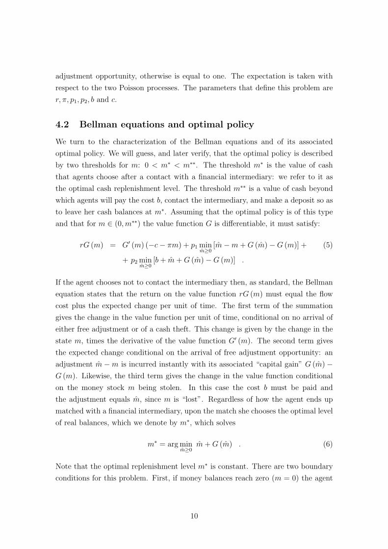
4.2 Bellman equations and optimal policy

We turn to the characterization of the Bellman equations and of its associated

optimal policy. We will guess, and later verify, that the optimal policy is described

by two thresholds for m: 0 < m∗ < m∗∗. The threshold m∗ is the value of cash

that agents choose after a contact with a financial intermediary: we refer to it as

the optimal cash replenishment level. The threshold m∗∗ is a value of cash beyond

which agents will pay the cost b, contact the intermediary, and make a deposit so as

to leave her cash balances at m∗. Assuming that the optimal policy is of this type

and that for m ∈ (0,m∗∗) the value function G is differentiable, it must satisfy:

rG (m) = G′ (m) (−c− πm) + p1 minm̂≥0

[m̂−m + G (m̂)−G (m)] + (5)

+ p2 minm̂≥0

[b + m̂ + G (m̂)−G (m)] .

If the agent chooses not to contact the intermediary then, as standard, the Bellman

equation states that the return on the value function rG (m) must equal the flow

cost plus the expected change per unit of time. The first term of the summation

gives the change in the value function per unit of time, conditional on no arrival of

either free adjustment or of a cash theft. This change is given by the change in the

state m, times the derivative of the value function G′ (m). The second term gives

the expected change conditional on the arrival of free adjustment opportunity: an

adjustment m̂−m is incurred instantly with its associated “capital gain” G (m̂)−G (m). Likewise, the third term gives the change in the value function conditional

on the money stock m being stolen. In this case the cost b must be paid and

the adjustment equals m̂, since m is “lost”. Regardless of how the agent ends up

matched with a financial intermediary, upon the match she chooses the optimal level

of real balances, which we denote by m∗, which solves

m∗ = arg minm̂≥0

m̂ + G (m̂) . (6)

Note that the optimal replenishment level m∗ is constant. There are two boundary

conditions for this problem. First, if money balances reach zero (m = 0) the agent

10

must withdraw, otherwise she will violate the non-negativity constraint in the next

instant. Second, for values of m ≥ m∗∗ we conjecture that the agent chooses to pay

b and deposit the extra amount, m − m∗. Combining these boundary conditions

with (5) we have:

G (m) =

b + m∗ + G (m∗) if m = 0−G′ (m) (c + πm) + (p1 + p2) [m∗ + G (m∗)] + p2b− p1m

r + p1 + p2

if m ∈ (0,m∗∗)

b + m∗ −m + G (m∗) if m ≥ m∗∗

(7)

For the assumed configuration to be optimal it must be the case that the agent

prefers not to pay the cost b and adjust money balances in the relevant range:

m + G (m) < b + m∗ + G (m∗) all m ∈ (0,m∗∗) . (8)

Summarizing, we say that m∗,m∗∗, G (·) solve the Bellman equation for the total

cost problem (4) if they satisfy (6)-(7)-(8).

We find it convenient to reformulate this problem so that it is closer to the

standard inventory theoretical models. We define a related problem where the agent

minimizes the shadow cost

V (m) = min{m(t),τj}

E0

{ ∞∑j=0

e−rτj

[Iτj

b +

∫ τj+1−τj

0

e−rtR m (t + τj) dt

]}(9)

subject to (3), m (t) ≥ 0, where τj denote the stopping times at which an adjustment

(jump) of m takes place, and m (0) = m is given. The indicator Iτjequals zero if

the adjustment takes place at the time of a free adjustment, otherwise is equal to

one. In this formulation R is the opportunity cost of holding cash. In this problem

there is only one Poisson process with intensity p describing the arrival of a free

opportunity to adjust. The parameters of this problem are r, R, π, p, b and c.7

The derivation of the Bellman equation for an agent unmatched with a financial

intermediary and holding a real value of cash m follows by the same logic used

7The shadow cost formulation is the standard one used in the literature for inventory theoreticalmodels, as in the models of Baumol-Tobin, Miller and Orr (1966), Constantinides (1976), amongothers. In these papers the problem aims to minimize the steady state cost implied by a station-ary inventory policy. This differs from our formulation, where the agent minimizes the expecteddiscounted cost in (9). In this regard our analysis follows the one of Constantinides and Richards(1978). For a related model, Frenkel and Jovanovic (1980) compare the resulting money demandarising from minimizing the steady state vs. the expected discounted cost.

11

to derive equation (5). The only decision that the agent must make is whether

to remain unmatched, or to pay the fixed cost b and be matched with a financial

intermediary. Denoting by V ′ (m) the derivative of V (m) with respect to m, the

Bellman equation satisfies

rV (m) = Rm + p minm̂≥0

(V (m̂)− V (m)) + V ′ (m) (−c−mπ) . (10)

Regardless of how the agent ends up matched with a financial intermediary, she

chooses the optimal adjustment and sets m = m∗, or

V ∗ ≡ V (m∗) = minm̂≥0

V (m̂) . (11)

As in problem (4) we will guess that the optimal policy is described by two

threshold values satisfying 0 < m∗ < m∗∗. This requires two boundary conditions.

At m = 0 the agent must pay the cost b and withdraw, and for m ≥ m∗∗ the agent

chooses to pay the cost b and deposit the cash in excess of m∗.8 Combining these

boundary conditions with (10) we have:

V (m) =

V ∗ + b if m = 0Rm + pV ∗ − V ′ (m) (c + mπ)

r + pif m ∈ (0,m∗∗)

V ∗ + b if m ≥ m∗∗

(12)

To ensure that it is optimal not to pay the cost and contact the intermediary in the

relevant range we require:

V (m) < V ∗ + b for m ∈ (0,m∗∗) . (13)

Summarizing, we say that m∗,m∗∗, V ∗, V (·) solve the Bellman equation for the

shadow cost problem (9) if they satisfy (11)-(12)-(13). We are now ready to show

that, first, (4) and (9) are equivalent and, second, the existence and characterization

of the solution.

Proposition 1. Assume that the opportunity cost is given by R = r + π + p2, andthat the contact rate with the financial intermediary is p = p1 + p2. Assume that the

8Since withdrawals are the agent only source of cash in this economy, in the invariant distributionof money holdings the threshold m∗∗ is never reached and all agents are distributed on the interval(0,m∗).

12

functions G (·) , V (·) satisfy

G (m) = V (m)−m + c/r + p2b/r (14)

for all m ≥ 0. Then, m∗,m∗∗, G (·) solve the Bellman equation for the total costproblem (4) if and only if m∗,m∗∗, V ∗, V (·) solve the Bellman equation for theshadow cost problem (9).Proof. See Appendix A.

We briefly comment on the relation between the total and shadow cost problems.

Notice that they are described by the same number of parameters. They have

r, π, c, b in common, the total cost problem uses p1 and p2, while the shadow cost

problem uses R and p. That R = r + π + p2 is quite intuitive: the shadow cost of

holding money is given by the real opportunity cost of investing, r, plus the fact

that cash holdings loose real value continually at a rate π and they are lost entirely

with probability p2 per unit of time. Likewise that p = p1 + p2 is clear too: since

the effect of either shock is to force an adjustment on cash. The relation between

G and V in (14) is quite intuitive. First the constant c/r is required, since even

if withdrawals were free (say b = 0) consumption expenditures must be financed.

Second, the constant p2b/r is the present value of all the withdrawals cost that is

paid after cash is “lost”. This adjustment is required because in the shadow cost

problem there is no theft. Third, the term m has to be subtracted from V since this

amount has already been withdrawn from the interest bearing account.

From now on, we use the shadow cost formulation, since it is closer to the

standard inventory decision problem. On the theoretical side, having the effect of

theft as part of the opportunity cost allows us to parameterize R as being, at least

conceptually, independent of r and π. On the quantitative side we think that, at

least for low nominal interest rates, the presence of other opportunity costs may be

important.

4.3 Characterization of the optimal return point m∗

The next proposition gives one non-linear equation whose unique solution determines

the cash replenishment value m∗ as a function of the model parameters: R, π, r, p, c

and b.

Proposition 2. Assume that r + π + p > 0. The optimal return point m∗c

has threearguments: β, r + p, π, where β ≡ b

cR. The return point m∗ is given by the unique

13

positive solution to

(m∗

cπ + 1

)1+ r+pπ

=m∗

c(r + p + π) + 1 + (r + p) (r + p + π)

b

cR. (15)

Proof. See Appendix A.

Note that, keeping r and π fixed, the solution for m∗/c is a function of b/(cR),

as it is in the steady state money demand of Section 3. This immediately implies

that m∗ is homogenous of degree one in (c, b). The next proposition gives a closed

form solution for the function V (·), and the scalar V ∗ in terms of m∗.

Proposition 3. Assume that r + π + p > 0. Let m∗ be the solution of (15).(i) The value for the agents not matched with a financial institution, for m ∈(0,m∗∗), is given by the convex function:

V (m) =

[pV ∗ −Rc/ (r + p + π)

r + p

]+

[R

r + p + π

]m +

(c

r + p

)2

A[1 + π

m

c

]− r+pπ

(16)

where A = r+pc2

(R m∗ + (r + p) b + Rc

r+p+π

)> 0 .

For m = 0 or m ≥ m∗∗ : V (m) = V ∗ + b.(ii) The value for the agents matched with a financial institution, V ∗, is

V ∗ =R

rm∗ . (17)

Proof. See Appendix A.

The close relationship between the value function at zero cash and the optimal

return point V (0) = (R/r) m∗ + b derived in this proposition will be useful to

measure the gains of different financial arrangements. The next proposition uses

the characterization of the solution for m∗ to conduct some comparative statics.

Proposition 4. The optimal return point m∗ has the following properties:(i) m∗

cis increasing in b

cR, m∗

c= 0 as b

cR= 0 and m∗

c→∞ as b

cR→∞ .

(ii) For small bcR

, we can approximate m∗c

by the solution in BT model, or

m∗

c=

√2

b

cR+ o

(√b

cR

)

where o(z)/z → 0 as z → 0.(iii) Assuming that the Fisher equation holds, in that π = R − r, the elasticity of

14

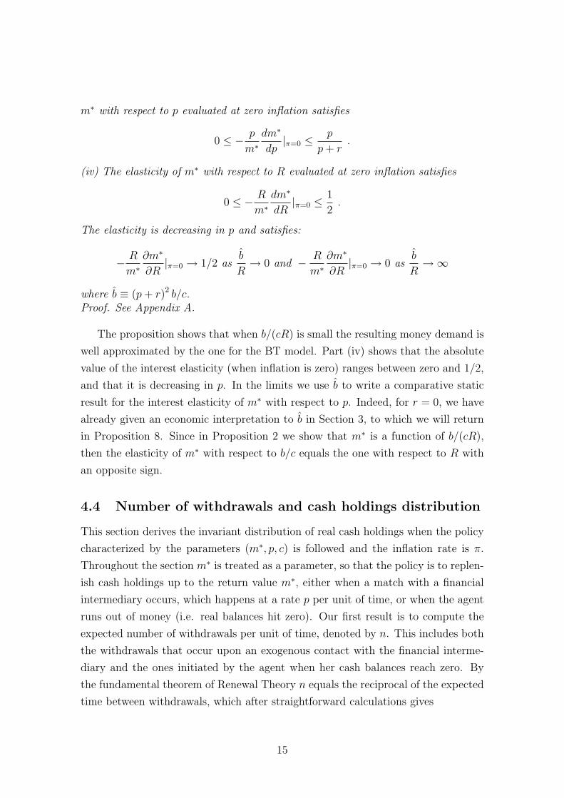
m∗ with respect to p evaluated at zero inflation satisfies

0 ≤ − p

m∗dm∗

dp|π=0 ≤ p

p + r.

(iv) The elasticity of m∗ with respect to R evaluated at zero inflation satisfies

0 ≤ − R

m∗dm∗

dR|π=0 ≤ 1

2.

The elasticity is decreasing in p and satisfies:

− R

m∗∂m∗

∂R|π=0 → 1/2 as

b̂

R→ 0 and − R

m∗∂m∗

∂R|π=0 → 0 as

b̂

R→∞

where b̂ ≡ (p + r)2 b/c.Proof. See Appendix A.

The proposition shows that when b/(cR) is small the resulting money demand is

well approximated by the one for the BT model. Part (iv) shows that the absolute

value of the interest elasticity (when inflation is zero) ranges between zero and 1/2,

and that it is decreasing in p. In the limits we use b̂ to write a comparative static

result for the interest elasticity of m∗ with respect to p. Indeed, for r = 0, we have

already given an economic interpretation to b̂ in Section 3, to which we will return

in Proposition 8. Since in Proposition 2 we show that m∗ is a function of b/(cR),

then the elasticity of m∗ with respect to b/c equals the one with respect to R with

an opposite sign.

4.4 Number of withdrawals and cash holdings distribution

This section derives the invariant distribution of real cash holdings when the policy

characterized by the parameters (m∗, p, c) is followed and the inflation rate is π.

Throughout the section m∗ is treated as a parameter, so that the policy is to replen-

ish cash holdings up to the return value m∗, either when a match with a financial

intermediary occurs, which happens at a rate p per unit of time, or when the agent

runs out of money (i.e. real balances hit zero). Our first result is to compute the

expected number of withdrawals per unit of time, denoted by n. This includes both

the withdrawals that occur upon an exogenous contact with the financial interme-

diary and the ones initiated by the agent when her cash balances reach zero. By

the fundamental theorem of Renewal Theory n equals the reciprocal of the expected

time between withdrawals, which after straightforward calculations gives

15

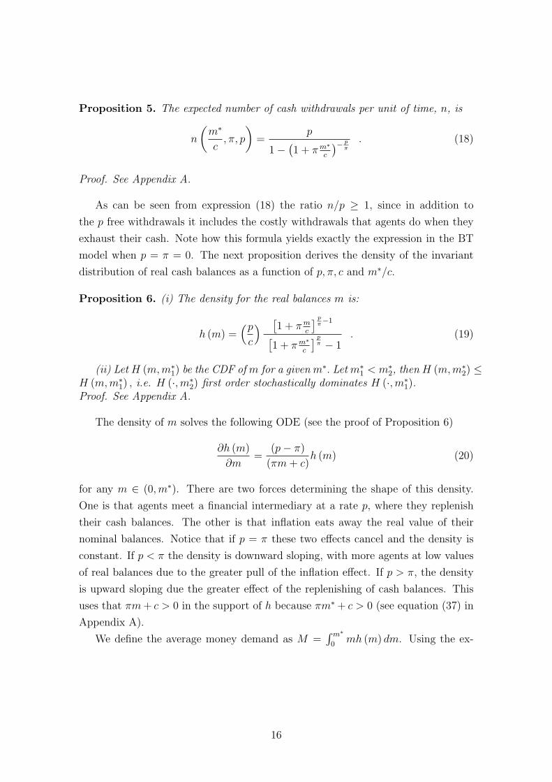
Proposition 5. The expected number of cash withdrawals per unit of time, n, is

n

(m∗

c, π, p

)=

p

1− (1 + πm∗

c

)− pπ

. (18)

Proof. See Appendix A.

As can be seen from expression (18) the ratio n/p ≥ 1, since in addition to

the p free withdrawals it includes the costly withdrawals that agents do when they

exhaust their cash. Note how this formula yields exactly the expression in the BT

model when p = π = 0. The next proposition derives the density of the invariant

distribution of real cash balances as a function of p, π, c and m∗/c.

Proposition 6. (i) The density for the real balances m is:

h (m) =(p

c

) [1 + πm

c

] pπ−1

[1 + πm∗

c

] pπ − 1

. (19)

(ii) Let H (m,m∗1) be the CDF of m for a given m∗. Let m∗

1 < m∗2, then H (m,m∗

2) ≤H (m,m∗

1) , i.e. H (·,m∗2) first order stochastically dominates H (·, m∗

1).Proof. See Appendix A.

The density of m solves the following ODE (see the proof of Proposition 6)

∂h (m)

∂m=

(p− π)

(πm + c)h (m) (20)

for any m ∈ (0, m∗). There are two forces determining the shape of this density.

One is that agents meet a financial intermediary at a rate p, where they replenish

their cash balances. The other is that inflation eats away the real value of their

nominal balances. Notice that if p = π these two effects cancel and the density is

constant. If p < π the density is downward sloping, with more agents at low values

of real balances due to the greater pull of the inflation effect. If p > π, the density

is upward sloping due the greater effect of the replenishing of cash balances. This

uses that πm + c > 0 in the support of h because πm∗ + c > 0 (see equation (37) in

Appendix A).

We define the average money demand as M =∫ m∗

0mh (m) dm. Using the ex-

16

pression for h(m), integration gives

M

c

(m∗

c, π, p

)=

(1 + πm∗

c

) pπ

[m∗c− (1+π m∗

c )p+π

]+ 1

p+π

[1 + πm∗

c

] pπ − 1

. (21)

Next we analyze how M depends on m∗ and p. The function Mc

(·, π, p) is increasing

in m∗, which follows immediately from part (ii) of Proposition 6: with a higher

target replenishment level the agents end up holding more money on average. The

next proposition shows that for a fixed m∗, M is increasing in p:

Proposition 7. The ratio Mm∗ is increasing in p with:

M

m∗ (π, p) =1

2for p = π and

M

m∗ (π, p) → 1 as p →∞.

Proof. See Appendix A.

It is useful to compare this result with the corresponding one for the BT case,

which is obtained when π = p = 0. In this case agents withdraw m∗ hence M/m∗ =

1/2. The other limit corresponds to the case where withdrawals happen so often

that at all times the average amount of money coincides with the amount just after

a withdrawal.

The average withdrawal, W , is

W = m∗[1− p

n

]+

[p

n

] ∫ m∗

0

(m∗ −m) h (m) dm . (22)

To understand the expression for W notice that (n−p) is the number of withdrawals

in a unit of time that occur because the zero balance is reached, so if we divide it by

the total number of withdrawals per unit of time (n) we obtain the fraction of with-

drawals that occur at a zero balance. Each of these withdrawals is of size m∗. The

complementary fraction gives the withdrawals that occur due to a chance meeting

with the intermediary. A withdrawal of size m∗−m happens with frequency h (m).

Inspection of (22) shows that W/c is a function of three arguments: m∗/c, π, p.

Combining the previous results we can see that for p ≥ π, the ratio of withdrawals

to average cash holdings is less than two. To see this, using the definition of W we

can writeW

M=

m∗

M− p

n. (23)

Since M/m∗ ≥ 1/2, then it follows that W/M ≤ 2. Indeed notice that for p

17

large enough this ratio can be smaller than one. We mention this property because

for the Baumol - Tobin model the ratio W/M is exactly two, while in the data of

Table 1 for households with an ATM card the average ratio is below 1.5 and its

median value is 1. The intuition for this result in our model is clear: agents take

advantage of the free random withdrawals regardless of their cash balances, hence

the withdrawals are distributed on [0,m∗], as opposed to be concentrated on m∗, as

in the BT model.

We let M be the average amount of money that an agent has at the time of

withdrawal. A fraction [1− p/n] of the withdrawals happens when m = 0. For the

remaining fraction, p/n, an agent has money holdings at the time of the withdrawal

distributed with density h, so that: M = 0 · [1− pn

]+

[pn

] ∫ m∗

0m h (m) dm . Inspec-

tion of this expression shows that M/c is a function of three arguments: m∗/c, π, p.

Simple algebra shows that M = m∗ −W or, inserting the definition of M into the

expression for M :

M =p

nM . (24)

The ratio M/M is a measure of the precautionary demand for cash: it is zero

only when p = 0, it goes to 1 as p → ∞ and, at least for π = 0, it is increasing

in p. This is because as p increases the agent has more opportunities for a free

withdrawal, which directly increases M/M (see equations 18 and 24), and from part

(iii) in Proposition 4 the induced effect of p on m∗ cannot outweigh the direct effect.

Other researchers noticing that currency holdings are positive at the time of

withdrawals account for this feature by adding a constant M/M to the sawtooth

path of a deterministic inventory model, which implies that the average cash balance

is M1 = M + 0.5 c/n or M2 = M + 0.5 W . See e.g. equations (1) and (2) in

Attanasio, Guiso and Jappelli (2002) and Table 1 in Porter and Judson (1996).

Instead, when we model the determinants of the precautionary holdings M/M in

a random setup, we find that W/2 < M < M + W/2. The leftmost inequality is

a consequence of Proposition 7 and equation (23), the other can be derived using

the form of the optimal decision rules and the law of motion of cash flows (see

the Online Appendix C). The discussion above shows that the expressions for the

demand for cash proposed in the literature to deal with the precautionary motive

are upward biased. Using the data of Table 1 shows that both expressions M1 and

M2 overestimate the average amount of cash held by Italian households by a large

margin.9

9The expression for M1 overestimates the average cash by 20% and 140% for household with

18

4.5 Comparative statics on M , M , W and welfare

We begin with a comparative statics exercise on M , M and W in terms of the

primitive parameters b/c, p, and R. To do this we combine the results of Section

4.3, where we analyzed how the optimal decision rule m∗/c depends on p, b/c and

R, with the results of Section 4.4 where we analyze how M , M , and W change as

a function of m∗/c and p. The next proposition defines a one dimensional index

b̂ ≡ (b/c)p2 that characterizes the shape of the money demand and the strength

of the precautionary motive focusing on π = r = 0. When r → 0 our problem is

equivalent to minimizing the steady state cost. The choice of π = r = 0 simplifies

the comparison of the analytical results with the ones for the original BT model and

with the ones of Section 3.

Proposition 8. Let π = 0 and r → 0, the ratios: W/M , M/M and (M/c) p aredetermined by three strictly monotone functions of b̂/R that satisfy:

Asb̂

R→ 0 :

W

M→ 2 ,

M

M→ 0 ,

∂ log Mpc

∂ log b̂R

→ 1

2.

Asb̂

R→∞ :

W

M→ 0 ,

M

M→ 1 ,

∂ log Mpc

∂ log b̂R

→ 0.

Proof. See Appendix A.

The elasticity of (M/c)p with respect to b̂/R determines the effect of the tech-

nological parameters b/c and p on the level of money demand, as well as on the

interest rate elasticity of M/c with respect to R since

η(b̂/R) ≡ ∂ log(M/c)p

∂ log(b̂/R)= −∂ log(M/c)

∂ log R. (25)

Direct computation gives that

∂ log(M/c)

∂ log p= −1 + 2η(b̂/R) ≤ 0 and 0 ≤ ∂ log(M/c)

∂ log(b/c)= η(b̂/R) . (26)

The previous sections showed that p has two opposing effects on M/c: for a given

m∗/c, the value of M/c increases with p, but the optimal choice of m∗/c decreases

with p. Proposition 8 and equation (26) show that the net effect is always negative.

For low values of b̂/R, where η ≈ 1/2, the elasticity of M/c with respect to p

and without ATMs, respectively; the one for M2 by 7% and 40%, respectively.

19

is close to zero and the one with respect to b/c is close to 1/2, which is the BT

case. For large values of b̂/R, the elasticity of M/c with respect to p goes to −1,

and the one with respect to b/c goes to zero. Likewise, equation (26) implies that

∂ log M/∂ log c = 1 − η and hence that the expenditure elasticity of the money

demand ranges between 1/2 (the BT value) and 1 as b̂/R becomes large.

In the original BT model W/M = 2, M/M = 0 and ∂ log(M/c)∂ log R

= −1/2 for

all b/c and R. These are the values that correspond to our model as b̂/R → 0.

This limit includes the standard case where p → 0, but it also includes the case

where b/c is much smaller than p2/R. As b̂/R grows, our model predicts smaller

interest rate elasticity than the BT model, and in the limit, as b̂/R →∞, that the

elasticity goes to zero. This result is a smooth version of the one for the model

with p deterministic free withdrawal opportunities of Section 3. In that model the

elasticity ∂ log(Mp/c)/∂ log(b̂/R) is a step function that takes two values, 1/2 for

low values of b̂/R, and zero otherwise. The smoothness is a natural consequence of

the randomness on the free withdrawal opportunities. One key difference is that the

deterministic model of Section 3 has no precautionary motive for money demand,

hence W/M =2 and M/M = 0. Instead, as Proposition 8 shows, in the model with

random free withdrawal opportunities, the strength of the precautionary motive, as

measured by W/M and M/M , is a function of b̂/R.

Figure 1 plots W/M , M/M and η as functions of b̂/R. This figure completely

characterizes the shape of the money demand and the strength of the precautionary

motive since the functions plotted in it depend only on b̂/R. The range of the b̂/R

values used in this figure is chosen to span the variation of the estimates presented in

Table 6. While this figure is based on results for π = r = 0, the figure obtained using

the values of π and r that correspond to the averages for Italy during 1993-2004 is

quantitatively indistinguishable.

We conclude this section with a result on the welfare cost of inflation and

the effect technological change. Let (R, κ) be the vector of parameters that in-

dex the value function V (m; R, κ) and the invariant distribution h(m; R, κ), where

κ = (π, r, b, p, c). We define the average flow cost of cash purchases borne

by households v(R, κ) ≡ ∫ m∗

0rV (m; R, κ)h(m; R, κ)dm. We measure the benefit of

lower inflation for households, say as captured by a lower R and π, or of a better

technology, say as captured by a lower b/c or a higher p, by comparing v(·) for the

corresponding values of (R, κ). A related concept is `(R, κ), the expected withdrawal

20

Figure 1: W/M , M/M , m∗/M and η = elasticity of (M/c)p

0 1 2 3 4 5 60.2

0.4

0.6

0.8

1

1.2

1.4

1.6

1.8

2For π = 0 and r −> 0

(b/c) p2 / R

W/M

Mlow/M

η = Elast (M/c)p

m*/M

ηW/MMlow/Mm*/M

cost borne by households that follow the optimal rule

`(R, κ) = [n(m∗(R, κ), p, π)− p] · b (27)

where n is given in (18) and the expected number of free withdrawals, p, are sub-

tracted. The value of `(R, κ) measures the resources wasted trying to economize on

cash balances, i.e. the deadweight loss for the society corresponding to R. While `

is the relevant measure of the cost for the society, we find useful to define v sepa-

rately to measure the consumers’ benefit of using ATM cards. The next proposition

characterizes `(R, κ) and v(R, κ) as r → 0. This limit is useful for comparison with

the BT model and it also turns out to be an excellent approximation for the values

of r that we use in our estimation.

Proposition 9. Let r → 0: (i) v(R, κ) = R m∗(R, κ); (ii) v(R, κ) =∫ R

0M(R̃, κ)dR̃,

and (iii) `(R, κ) = v(R, κ)−R M(R, κ).Proof. See Appendix A.

This proposition allows us to estimate the effect of inflation or technology on agents’

welfare using data on W and M , since W + M = m∗. In the BT model ` = RM =

21

√Rbc/2 since m∗ = W = 2M . In our model m∗/M = W/M + M/M < 2, as

can be seen in Figure 1, thus using RM as an estimate of R(m∗ −M) produces an

overestimate of the cost of inflation `. For instance, for b̂/R = 1.8, the BT welfare

cost measure overestimates the cost of inflation by about 67%, since m∗/M ∼= 1.6.

Clearly the loss for society is smaller than the cost for households; using (i)-(iii)

and Figure 1 the two can be easily compared. As b̂/R ranges from zero to ∞, the

ratio of the costs `/v decreases from 1/2, the BT value, to zero. Not surprisingly

(ii)-(iii) implies that the loss for society coincides with the consumer surplus that can

be gained by reducing R to zero, i.e. `(R) =∫ R

0M(R̃)dR̃ − RM(R). This extends

the result of Lucas (2000), derived from a money-in-the-utility-function model, to an

explicit inventory-theoretic model. Measuring the welfare cost of inflation using the

consumer surplus requires the estimation of the money demand for different interest

rates, while the approach using (i) and (iii) can be done using information on M ,

W and M . Section 7 presents an application of these results and a comparison with

the ones by Lucas (2000).10

5 Estimation of the model

We estimate the parameters (p, b/c) using the data described in Section 2 under two

alternative sets of assumptions. Our baseline assumptions are that all households in

the same cell (to be defined below) have the same parameters (p, b/c). For this case

we discuss the identification of the parameters and the goodness of fit of the model.

Alternatively in Section 5.3 we assume that (p, b/c) are a simple parametric function

of individual household characteristics. In both cases we take the opportunity cost

R as observable (see Table 2), and assume that households values of (M/c, n, W/M ,

M/M) are observed with classical normally distributed measurement error (in logs).

The assumption of classical measurement error is often used when estimating

models based on household survey data. We find that the pattern of violations

of a simple accounting identity, c = n W − πM , is consistent with large classical

measurement error. In particular, a histogram of the deviations of this identity (in

log points) is centered around zero, symmetric, and roughly bell shaped (see the

Online Appendix J for more details).

Let us provide a complete list of the assumptions used in the baseline estimation.

We define a cell as a particular combination of year-province-household type, where

10In (ii)-(iii) we measure welfare and consumer surplus with respect to variations in R, keepingπ fixed. The effect on M and v of changes in π for a constant R are quantitatively small.

22

the latter is defined by the cash expenditure third-tile and ATM ownership. This

yields about 3,700 cells, the product of the 103 provinces of Italy × 6 time periods

(spanning 1993-2004) × 2 ATM ownership status (whether a household has an

ATM card or not) × 3 cash consumption third-tiles. For each year we observed

the inflation rate π, and for each year-province-ATM ownership type we observed

the opportunity cost R. Let i index the households in a cell. For all households

in that cell we assume that bi/ci and pi are identical. Given the homogeneity of

the optimal decision rules, this implies that all household i have the same values of

M/c, W/M, n, M/M .

Let j = 1, 2, 3, 4 index the variables M/c, W/M , n and M/M , let zji be the (log

of the) i− th household observation on variable j, and ζj (θ) the (log of the) model

prediction of the j variable for the parameter vector θ ≡ (p, b/c). The variable

zji is observed with a zero-mean measurement error εj

i with variance σ2j , so that

zji = ζj (θ) + εj

i . It is assumed that the parameter σ2j is common across cells (we

allow one set of variances for households with ATM cards, and one for those without).

The estimation proceeds in two steps. We first estimate σ2j by regressing each

of the 4 observables, measured at the individual household level, on a vector of cell

dummies. The variance of the regression residual is our estimate of σ2j (there are

about 20,000 degrees of freedom for each estimate). Since the errors εji are assumed

to be independent across households i and variables j, we estimate the vector of

parameters θ for each cell separately, by minimizing the likelihood criterion

F (θ; z) ≡4∑

j=1

(Nj

σ2j

) 1

Nj

Nj∑i=1

zji − ζj (θ)

2

(28)

where σ2j is the measurement error variance estimated above and Nj is the sample

size of the variable j.11 Minimizing F (for each cell) yields the maximum likelihood

estimator provided the εji are independent across j for each i.

11The average number of observations (Nj) available for each variable varies. It is similar forhouseholds with and without ATM cards. There are more observations on M/c than for eachof the other variables, and its average weight (N1/σ2

1) is about 1.5 times larger than each of theother three weights (see the Online Appendix L8 for further documentation). The number ofhouseholds-year-type combinations used to construct all the cells is approximately 40, 000.

23

5.1 Estimation and Identification

In this section we discuss the features of the data that identify our parameters.

We argue that with our data set we can identify(p, b

cR

). As a first step we

study how to select the parameters to match M/c and n only, as opposed to

(M/c, n, W/M, M/M). To simplify the exposition assume zero inflation, π = 0.

For the BT model, i.e. for p = 0, we have W = m∗, c = m∗ n and M = m∗/2

which implies 2 M/c = 1/ n. Hence, if the data were generated by the BT model,

M/c and n would have to satisfy this relation. Now consider the average cash bal-

ances generated by a policy like the one of the model of Section 4. From (18) and

(21), for a given value of p and setting π = 0, we have:

M

c=

1

p[n m∗/c− 1] and n =

p

1− exp (−pm∗/c)(29)

or, solving for M/c as a function of n :

M

c= ξ (n, p) =

1

p

[−n

plog

(1− p

n

)− 1

]. (30)

For a given p, the pairs M/c = ξ (n, p) and n are consistent with a cash management

policy of replenishing balances to some value m∗ either when the zero balance is

reached or when a chance meeting with an intermediary occurs. Notice first that

setting p = 0 in this equation we obtain BT, i.e. ξ (n, 0) = (1/2) /n. Second, notice

that this function is defined only for n ≥ p. Furthermore, note that for p > 0 :∂ξ∂n≤ 0, ∂2ξ

∂n2 > 0, and ∂ξ∂p

> 0. Consider plotting the target value of the data on

the (n, M/c) plane. For a given M/c, there is a minimum n that the model can

generate, namely the value (1/2) / (M/c). Given that ∂ξ/∂p > 0, any value of n

smaller than the one implied by the BT model cannot be made consistent with our

model, regardless of the values for the rest of the parameters. By the same reason,

any value of n higher than (1/2) / (M/c) can be accommodated by an appropriate

choice of p. This is quite intuitive: relative to the BT model, our model can generate

a larger number of withdrawals for the same M/c if the agent meets an intermediary

often enough, i.e. if p is large enough. On the other hand there is a minimum number

of expected chance meetings, namely p = 0.

The previous discussion showed that p is identified. Specifically, fix a province-

year-type of household combination, with its corresponding values for M/c and n.

Then, solving M/c = ξ (n, p ) for p gives an estimate of p. Taking this value of p, and

24

those of M/c and n for this province-year-type combination, we use (29) to solve for

m∗/c. Finally, we find the value of β ≡ b/ (cR) consistent with this replenishment

target by solving the equation for m∗ given in Proposition 2,

β ≡ b

cR=

exp [(r + p) m∗/c]− [1 + (r + p) (m∗/c)]

(r + p)2 . (31)

To understand this expression consider two pairs (M/c, n), both on the locus defined

by ξ (·, p) for a given value of p. The pair with higher M/c and lower n corresponds

to a higher value of β. This is quite simple: agents will economize on trips to the

financial intermediary if β is high, i.e. if these trips are expensive relative to the

opportunity cost of cash. Hence, data on M/c and n identify p and β. Using data

on R for this province-year, we can estimate b/c.

Figure 2 plots the function ξ (·, p) for several values of p, as well as the aver-

age value of M/c and n for all households of a given type (i.e. with and without

ATM cards) for each province-year in our data (to make the graph easier to read

we do not plot different consumption cells for a given province-year-ATM owner-

ship). Notice that 46 percent of province-year pairs for households without an ATM

card are below the ξ (·, 0) line, so no parameters in our model can rationalize those

choices. The corresponding value for those with an ATM card is only 3.5 percent

of the pairs. The values of p required to rationalize the average choice for most

province-year pairs for those households without ATM cards are in the range p = 0

to p = 20. The corresponding range for those with ATM cards is between p = 5

and p = 60. Inspecting this figure we can also see that the observations for house-

holds with ATM cards are to the south-east of those for households without ATM

cards. Equivalently, we can see that for the same value of p, the observations that

correspond to households with ATM tend to have lower values of β.

We now show that the pair of observables W/M and n also allows on to identify

the model structural parameters. As in the previous case, consider an agent that

follows an arbitrary policy of replenishing her cash to a return level m∗, either as

her cash balances hit zero, or at the time of chance meeting with the intermediary.

Again, to simplify consider the case of π = 0. Using the cash flow identity nW = c

and (30) yields

W

M= δ (n, p) ≡

[1

p/n+

1

log (1− p/n)

]−1

− p

n(32)

25

Figure 2: Theory vs. data (province-year mean): M/c, n

1 1.5 2 2.5 3 3.5 4 4.5

−4.5

−4

−3.5

−3

−2.5

−2

Theory (solid lines) vs Data (dots)dot size = # obs, empty = HHs w/o ATM, filled = HHs w/ATM

M/c

: av

erag

e ca

sh b

alan

ce o

ver d

aily

cas

h ex

pend

iture

(in

logs

)

n: number of withdrawals per year (in logs)

p = 0Baumol−Tobin

p = 5 p = 10 p = 20 p = 35 p = 60

for n ≥ p, and p ≥ 0. Some algebra shows that

δ (n, 0) = 2, δ (n, n) = 0 ,∂δ (n; p)

∂p< 0 ,

∂δ (n; p)

∂n> 0.

Notice that the ratio W/M is a function only of the ratio p/n. The interpretation of

this is clear: for p = 0 we have W/M = 2, as in the BT model. This is the highest

value that can be achieved by the ratio W/M . As p increases for a fixed n, the

replenishing level of cash m∗/c must be smaller, and hence the average withdrawal

becomes smaller relative the average cash holdings M/c. Indeed, as n converges to

p −a case where almost all the withdrawals are due to chance meetings with the

intermediary−, then W/M goes to zero. As in the previous case, given a pair of

observations on W/M and n, we can use δ to solve for the corresponding p. Then,

using the values of (W/M p, n) we can find a value of (b/c) /R to rationalize the

choice of W/M . To see how, notice that given W/M, M/c, and p/n, we can find

the value of m∗/c using WM

= m∗/cM/c

− pn

(equation 23). With the values of (m∗/c, p)

we can find the unique value of β = (b/c) /R that rationalizes this choice, using

(31). Thus, data on W/M and n identifies p. The implied values of p needed to

26

rationalize these data are similar to the ones found using the information of M/c

and n displayed in Figure 2.

Finally notice that the ratio M/M can also be used to identify the model struc-

tural parameters. In (24) we have derived that p = n (M/M). We use this

equation as a way to estimate p. If M is zero, then p must be zero. Hence the fact

that M/M > 0, documented in Table 1, is an indication that our model requires

p > 0. We can readily use this equation to estimate p since we have data on both n

and (M/M). According to this formula a large value of p is consistent with either

a large ratio of cash at withdrawals, M/M , or a large number of withdrawals, n.

Also, for a fixed p, different combinations of n and M/M that give the same product

are due to differences in β = (b/c) /R. If β is high, then agents economize on the

number of withdrawals and keep larger cash balances (see the Online Appendix L9

for more documentation).

We have discussed how data on any of the pairs (M/c, n), (W/M,n) or (M/M,n)

identify p and β. Of course, if the data had been generated by the model, the three

ways of estimating (p, β) would produce identical estimates. In other words, the

model is overidentified. We will use this idea to report how well the model fits the

data or, more formally, to test for the overidentifying restrictions in the next section.

Considering the case of π > 0 makes the expressions more complex, but, at least

qualitatively, does not change any of the properties discussed above. Moreover, since

the inflation rate in our data set is quite low the expressions for π = 0 approximate

the relevant range for π > 0 very well.

5.2 Estimation results

We estimate the model for each province-year-type of household and report statistics

of the estimates in Table 3. For each year we use the inflation rate corresponding

to the Italian CPI for all provinces and fix the real return r to be 2% per year.

The first two panels in the table report the mean, median, 95th and 5th percentile

of the estimated values for p and b/c across all province-year. As explained above,

our procedure estimates β ≡ bc R

, so to obtain b/c we compute the opportunity cost

R as the sum of the nominal interest rate and the probability of cash being stolen

described in Table 2. The parameter p gives the average number of free withdrawals

opportunities per year. The parameter b/c · 100 is the cost of a withdrawal in

percentage of the daily cash-expenditure. We also report the mean value of the t

statistics for these parameters. The asymptotic standard errors are computed by

27

solving for the information matrix.

Table 3: Summary of (p, b/c) estimates across province-year-types

Household w/o ATM Household w. ATMCash expenditurea: Low High Low High

Parameter pMean 6.8 8.7 20 25Median 5.6 6.2 17 2095thpercentile 17 25 49 615th percentile 1.1 0.8 3 4Mean t-stat 2.5 2.2 2.7 3.5

Parameter b/c (in % of daily cash expenditure)Mean 10.5 5.5 6.5 2.1Median 7.3 3.6 3.5 1.195th percentile 30 17 24 75th percentile 1.5 0.4 0.6 0.3Mean t-stat 2.8 2.5 2.4 3.3

# prov-year-type estimates 504 505 525 569

Goodness of fit: Likelihood Criterion F (θ, x) ∼ χ2

% province-years-type where:- F (θ, x) < 4.6b 64% 57%

# prov-year-type estimates 1,539 1,654Avg. # of households per estimate 10.7 13.5

Notes: - a Low (high) denotes the lowest (highest) third of households ranked by cash expenditurec. - b Percentage of province-year-type estimates where the overidentifying restriction test is notrejected at the 10 per cent confidence level.

The results reported in the first two columns of the table concern households

who posses an ATM card, shown separately for those in the lowest and highest

cash expenditure levels. The corresponding statistics for households without ATM

card appear in the third and fourth columns. The results in this table confirm the

graphical analysis of figure 2 discussed above: the median estimates of p are just

where one would locate them by the figures. The difference between the 95th and the

5th percentiles indicates that there is a tremendous amount of heterogeneity across

province-years. The relatively low values for the mean t-statistics reflect the fact

that the number of households used in each estimation cell is small. Indeed, in the

Online Appendix I we consider different levels of aggregation and data selection. In

all the cases considered we find very similar values for the average of the parameters

p and b/c, and we find that when we do not disaggregate the data so much the

28

average t-stats increase roughly with the (square root) of the average number of

observations per cell.12

Table 3 shows that the average value of b/c across all province-year-type is be-

tween 2 and 10 per cent of daily cash consumption. Fixing an ATM ownership type,

and comparing the average estimates for p and b/c across cash consumption cells

we see that there are small differences for p, but that b/c is substantially smaller for

the those in the highest cash consumption cell. Indeed, combining this information

with the level of cash consumption that corresponds to each cell we estimate b to

be uncorrelated with cash consumption levels, as documented in Section 6. Using

information from Table 1 for the corresponding cash expenditure to which these per-

centages refer, the mean values of b for households with and without ATM are 0.8

and 1.7 euros at year 2004 prices, respectively. For comparison, the cash withdrawal

charge for own-bank transactions was zero, while the average charge for other-bank

transactions, which account for less than 20 % of the total, was 2.0 euros.13

Next we discuss three different types of evidence that indicate a successful em-

pirical performance of the model. First, Table 3 shows that households with ATM

cards have a higher mean and median value of p and correspondingly lower values

of b/c. The comparison of the (p, b/c) estimates across province-year-consumption

cells shows that 88 percent of the estimated values of p are higher for households

with ATM, and for 82 percent of the estimated values of b/c are lower. Also, there

is evidence of an effect at the level of the province-year-consumption cell, since we

find that the correlation between the estimated values of b/c for households with

and without ATM across province-year-consumption cell is 0.69. The same statis-

tic for p is 0.3. These patterns are consistent with the hypothesis that households

with ATM cards have access to a more efficient transactions system, and that the

efficiency of the transaction technology in a given province-year-consumption cell

is correlated for both ATM and non-ATM adopters. We find this result reassuring

since we have estimated the model for ATM holders and non-holders and for each

province-year-consumption cell separately.

Second, in the third panel of Table 3 we report statistics on the goodness of fit

of the model. For each province-year-type cell, under the assumption of normally

12Concerning aggregation, we repeat all the estimates without disaggregating by the level ofcash consumption, so that Nj is three times larger. Concerning data selection, we repeat all theestimates excluding those observations where the cash holding identity is violated by more than200% or where the share of total income received in cash by the household exceeds 50%. Thegoal of this data selection, that roughly halves the sample size, is to explore the robustness of theestimates to measurement error.

13The sources are Retail Banking Research (2005) and an internal report by the Bank of Italy.

29

distributed errors, or as an asymptotic result, the minimized likelihood criterion is

distributed as a χ2(2). According to the statistic reported in the first line of this

panel, in more than half of the province-years-consumption cells the minimized like-

lihood criterion is smaller than the critical value corresponding to a 10% probability

confidence level.

Table 4: Correlations between (p, bc, V (0)) estimates and financial diffusion indices

Household with ATMp b/c V (0)

Bank-branch per 1,000 head 0.08 -0.19 -0.18ATM per 1,000 head 0.10 -0.27 -0.27

Household with No ATMp b/c V (0)

Bank-branch per 1,000 head 0.00a -0.26 -0.20

Notes: All variables are measured in logs. The sample size is 1,654 for HH w. ATM and1,539 for HH without ATM. P-values for the null Hp. of a zero coefficient (not reported),computed assuming that the estimates are independent, are smaller than 1 per cent withthe exception of the one denoted by a.

Third, in Table 4 we compute correlations of the estimates of the technological

parameters p, b/c and the cost of financing cash purchases V (0) with indicators

that measure the density of financial intermediaries: bank branches and ATMs per

resident that vary across province and years. A greater financial diffusion raises

the chances of a free withdrawal opportunity (p)and reduces the cost of contacting

an intermediary (b/c). Hence we expect V (0) to be negatively correlated with the

diffusion measure. We find that the estimates of b/c and V (0) are negatively corre-

lated with these measures, and that the estimated p are positively correlated, though

the latter correlation is smaller. This finding is reassuring since the indicators of

financial diffusion were not used in the estimation of (p, b/c).

5.3 Estimates using individual household data

This section explores an alternative estimation strategy based on individual house-

hold observations. It is assumed that the four variables (M/c, W/M , n, M/M)

are observed with classical measurement error, and that the parameters b/c and p

differ for each households, and are given by a simple function of household level

variables. In particular, let Xi be a k dimensional vector containing the value of

households i covariates. We assume that for each household i the values of b/c and

30

p are given by (b/c)i = exp(λb/c · Xi

)and pi = exp (λp · Xi), where λp are λb/c

are the parameters to be estimated. The vector Xi contains k = 8 covariates: a

constant, calendar year, the household cash expenditure (in logs), an ATM dummy,

a measure of the financial diffusion of Bank Branches and ATM terminals at the

province level, a credit card dummy, the income level per adult (in logs), and the

household size.

Assuming that the measurement error is independent across households and

variables, the maximum likelihood estimate of λ minimizes

F (λ, X) ≡4∑

j=1

1

σ2j

N∑i=1

[zj

i − ζj( θ(λ,Xi, Ri) )]2

where, as above, zji is the log of the j-th observable for household i, ζj(θ) is the

model solution given the parameters θ and N is the number of households in the

sample.14 The estimation proceeds in two steps. We first estimate σ2j for each of the

4 variables by running a regression at the household level of each of the 4 variables

against the household level Xi. We then minimize the likelihood criterion F taking

the estimated σ̂2j as given. The asymptotic standard errors of λ are computed by

inverting the information matrix.

Table 5 presents the estimates of λ. The first column displays the point estimates

of λp and the fourth the point estimates for λb/c. The number in parenthesis next

to the point estimates are the corresponding t-stats. To compare the results with

the benchmark estimates of Section 5.2 the table also includes the coefficients of

two regressions, under the labels λ̄p and λ̄b/c. The dependent variables of these

regression are the benchmark estimates of p and b/c, and hence they are the same for

all households in a cell −i.e. combination of a year, province, ATM card ownership,

and third-tile cash consumption−, the right hand side variables are the cell-means

of the Xi covariates.

We now discuss the estimation results. The estimates of p and b/c that corre-

spond to a household with the average values of each of the Xi variables and our

estimated parameters λp and λb/c are, respectively, 11 and 5.2 percent. These two

values are similar to the estimates reported in Table 3 (in particular they are close

14Notice that we treat the opportunity cost Ri as known. To speed up the calculations weestimate the model assuming that inflation is zero. Based on the results for our benchmark casewe think this will have at most a very minor effect on the estimates. We also restrict the sampleto households that have information for all the 4 variables of interest, this gives us a sample ofabout N = 17, 000 (as opposed to 40,000 in our benchmark estimates).

31

Table 5: Household level (p, b/c) estimates

Xi covariates λp t-stat λ̄p λb/c t-stat λ̄b/c

constant -87.7 (-1,370) -87.7 225 (3,340) 217year 0.04 (0.67) 0.04 -0.11 (-1.64) -0.11log cash expenditure 0.04 (0.03) -0.01 -0.96 (-0.62) -0.97ATM dummy 1.24 (64.70) 1.28 -0.66 (-32.7) -0.75log ATM and BB density -0.15 (-1.30) -0.16 -0.37 (-2.8) -0.34credit card dummy 0.30 (2.96) 0.21 -0.01 ( -0.05 ) 0.08log income 0.25 (4.18) 0.30 0.26 (4.05) 0.33log HH size 0.35 (4.05) 0.28 0.26 (2.74) 0.27

Notes: Estimates for p, b/c under the assumption that (b/c)i = exp(λb/cXi

)and pi =

exp (λpXi). Xi is at the household level and (M/c, W/M , n, M/M) measured with error.

to the median across cells). The mean estimate for p, greater than zero, supports

the introduction of this dimension of the technology, as opposed to having only the

BT parameter b/c. The estimates of both ATM dummies are economically impor-

tant, and statistically significant. Households with an ATM card are estimated to

have a value of p approximately three times bigger (exp(1.24) ≈ 3.46) and a value

of b/c about half (exp(−0.66) ≈ 0.52) relative to households without ATM cards.

There is a small positive time trend on p and a larger negative time trend on b/c,

although neither estimate is statistically significant. The value of b/c is smaller in

locations with higher density of ATM or Bank Branches with an elasticity of −0.37

borderline statistically significant, but this measure has a small negative effect on

p.15 The credit card dummy estimates suggest that the credit card has no effect on

b/c and a small positive borderline significant effect on p. A possible interpretation

for the effect on p is that households with a credit card have a better access to

financial intermediaries. We find a positive effect of the log of the household size

(number of adults) in both p and b/c. This result is hard to interpret. If the with-

drawal technology available to a households, summarized by (p, b/c), had increasing

(decreasing) returns with respect to household size, we would have expected the p

and b/c to vary in opposite way as the household size changed. The coefficient of

cash consumption indicates a small effect on p and an elasticity with respect to b/c

of almost negative one (−0.96), although it is imprecisely estimated (this elasticity

15Table 4 showed a positive, albeit small, correlation.

32

is very close to the one estimated using cell level aggregated data). The income per

adult has a positive elasticity of about 0.25 for both p and b/c. We interpret the

effect of income per capita on p as reflecting better access to financial intermedi-

aries, and with respect to b/c as measuring a higher opportunity cost of time. The

combination of the effects of income per capita and cash expenditures yields the

following important corollary: the value of b is estimated to be independent of the

level of cash expenditure of the household, implying a cash expenditure elasticity of

money demand approximately of one half provided that the opportunity cost of time

is the same.

We conclude by discussing a goodness of fit statistics. The value of the minimized

likelihood criterion is F = 62, 804, which equals half of the log-likelihood minus a

constant not involving λ. Under the assumption of independent measurement error

F is distributed as a χ2 with N × 4− 2× k = 54, 260 degrees of freedom in a large

sample.16 The minimized value for F reflects a relatively bad fit of the model. A

χ2 distribution with 54, 260 degrees of freedom gives essentially zero probability of

obtain such a large value. This is to be compared with the model estimated using

cell aggregated data, which passed the over-identifying restrictions test for more

than half of the cells (see Table 3).

6 Implications for money demand

In this section we study the implications of our findings for the time patterns of

technology and for the expenditure and interest elasticity of the demand for currency.

We begin by documenting the trends in the withdrawal technology, as measured

by our estimates of p and b/c. Table 6 shows that p has approximately doubled, and

that (b/c) has approximately halved over the sample period. In words, our point

estimates indicate that the withdrawal technology has improved through time.17 The

table also reports b̂/R ≡ (b/c)p2/R, which as shown in Proposition 8 and illustrated

in Figure 1 determines the elasticity of the money demand and the strength of the

precautionary motive. In particular, the proposition implies that W/M and M/M

depend only on b̂/R. The upward trend in the estimates of b̂/R, which is mostly

a reflection of the downward trend in the data for W/M , implies that the interest

rate elasticity of the money demand has decreased through time.

16We estimate k loadings λb/c and k loadings λp using N households with 4 observations each.17Since we have only 6 time periods, the time trend are imprecisely estimated, as it can be seen

from the t-stats corresponding to years in Table 5

33

Table 6: Time series pattern of estimated model parameters

1993 1995 1998 2000 2002 2004 All yearsHouseholds with ATM

p 17 16 20 24 22 33 22

b/c× 100 6.6 5.7 2.8 3.1 2.8 3.5 4.0

b̂/R 1.1 1.4 1.9 5.6 3.0 5.8 3.2

Households without ATMp 6 5 8 9 8 12 8

b/c× 100 13 12 6.2 4.9 4.5 5.7 7.7

b̂/R 0.2 0.2 0.4 0.4 0.4 1.6 0.5

R× 100 8.5 7.3 4.3 3.9 3.2 2.9 5.0

R and p are annual rates, c is the daily cash expenditure rate, and for each province-year-type b̂/R = b · p2/(365 · c ·R), which has no time dimension. Entries in the table are samplemeans across province-type in a year.

By Proposition 8, the interest rate elasticity η(b̂/R) implied by those estimates is

smaller than 1/2, the BT value. Using the mean of b̂/R reported in the last column

of Table 6 to evaluate the function η in Figure 1 yields values for the elasticity equal

to 0.43 and 0.48 for households with and without ATM card, respectively. Even for

the largest values of b̂/R recorded in Table 6, the value of η remains above 0.4. In

fact, further extending the range of Figure 1 it can be shown that values of b̂/R

close to 100 are required to obtain an elasticity η smaller than 0.25. For such high

values of b̂/R, the model implies M/M of about 0.99 and W/M below 0.3, values

reflecting much stronger precautionary demand for money than those observed for

most Italian households. On the other hand, studies using cross sectional household

data, such as Lippi and Secchi (2007) for Italian data, and Daniels and Murphy

(1994) using US data, report interest rate elasticities smaller than 0.25.

A possible explanation for the difference in the estimated elasticities is that the

cross sectional regressions in the studies mentioned above fail to include adequate

measures of financial innovations, and hence the estimate of the interest rate elas-

ticity is biased towards zero. To make this clear, in Table 7 we estimate the interest

elasticity of M/c by running two regressions for each household type where M/c is

the model fitted value for each province-year-consumption type. The first regression

includes the log of p, b/c and R. According to Proposition 8, (M/c) p has elasticity

34

η(b̂/R) so that we approximate it using a constant elasticity:

log M/c = − log p + η( log(b/c) + 2 log(p) )− η log(R) . (33)

The regression coefficient for η estimated from (33) gives virtually the same value

obtained from Figure 1. Since the left hand side of the equation uses the values

of M/c produced by the model using the estimated p, b/c and no measurement

error, the only reason why the regression R2 does not equal one is that we are

approximating a non-linear function with a linear one. Yet the R2 is pretty close

to one because the elasticity, for this range of parameters, is close to constant. To

estimate the size of the bias due to the omission of the variables log p and log b/c, the

second regression includes only log R. The regression coefficient for log R is an order

of magnitude smaller than the value of η, pointing to a large omitted variable bias:

the correlation between (log(b/c)+2 log(p)) and log R is 0.12 and 0.17 for households

with and without ATM card, respectively. Interestingly, the regression coefficients

on log R estimated by omitting the log of p and b/c are similar to the values that

are reported in the literature mentioned above. Replicating the regressions of Table

7 using the actual, as opposed to the fitted, value of M/c as a dependent variable

yields very similar results (not reported here).

Table 7: A laboratory experiment on the interest elasticity of money demand

Dependent variable: log(M/c) Household w. ATM Household w/o ATMlog(p) -0.05 - -0.01 -log(b/c) 0.45 - 0.48 -log(R) -0.44 -0.07 -0.48 -0.04R2 0.985 0.01 0.996 0.004# observations (cells) 1,654 1,654 1,539 1,539

Notes: All regressions include a constant.

We now estimate the expenditure elasticity of the money demand. An advantage

of our data is that we use direct measures of cash expenditures (as opposed to income

or wealth).18 By Proposition 8, the expenditure elasticity is

∂ log M

∂ log c= 1 + η(b̂/R)

∂ log b/c

∂ log c. (34)

For instance, if the ratio b/c is constant across values of c then the elasticity is one;

18Dotsey (1988) argues for the use of cash expenditure as the appropriate scale variable.

35

alternatively, if b/c decreases proportionately with c the elasticity is 1 − η. Using

the variation of the estimated b/c across time, locations and household groups with

different values of c, we estimate the elasticity of b/c with respect to c equal to

−0.82 and −1.01 for households without and with ATM card, respectively. Using the

estimates for η we obtain that the mean expenditure elasticity is 1+0.48×(−0.82) =

0.61 for households without ATM, and 0.56 for those with.

7 Cost of inflation and Benefits of ATM card

We use the estimates of (p, bc) to quantify the deadweight loss for the society and the

cost for households of financing cash purchases and to discuss the benefits of ATM

card ownership. In Section 4.5 we showed that the loss is ` = R(m∗ −M) and the

household cost is v = Rm∗. In the first panel of Table 8 we display the average of `

and of `/c for each year. In 1993 the loss is 24 euros or 0.99 days of cash purchases.

Table 8: Deadweight loss ` and household cost v of cash purchases

1993 1995 1998 2000 2002 2004 mean` (2004 euros, per household) 24 23 11 11 10 10 15

`/c (in days of cash purchases) 0.99 0.85 0.46 0.42 0.39 0.40 0.59

`/c under 1993 technology 0.99 0.90 0.72 0.71 0.67 0.66 0.78

v (2004 euros, per household) 51 49 25 25 22 25 33

v/c : avg. group / avg. all groups w. ATM w/o ATM- high c (top third ranked by c) 0.61 1.00- low c (bottom third ranked by c) 1.11 1.48

Note: ` and v are averages weighted by the number of household type, and measured asannual flows. The average value of v/c across all groups is 1.31 days of cash purchases.

To put this quantity in perspective we relate it to the one in Lucas (2000), obtained

by fitting a log-log money demand with an interest elasticity of 1/2, which corre-

sponds to the BT model. Figure 5 in his paper plots the welfare cost of inflation,

denoted by w (and defined as our `), which for an opportunity cost R of 5%, is about

1.1% of US GDP. At the same R our deadweight loss ` is about 14 times smaller,

or 0.08% of the annual income for Italian households y (c · 365 accounts for about

half of annual Italian GDP, `/y = 0.59/(2 · 365) ∼= 0.08%). There are two reasons

for this difference. The first is that for a given cost R and money demand M/c, the

deadweight loss in our model is smaller than in BT (see Section 4.5). For instance

36

for R = 0.05 and b̂/R = 1.8, which is about our sample average, w/` is about 1.6.

The second is that the welfare cost is proportional to the level of the money demand:

multiplying M/y by a constant, multiplies `/y by the same constant. In particular,

Lucas fits US data with a much higher value of M/y than the one we use for Italy:

0.225 versus 0.026 at R = 0.05. This is because while we focus on currency held by

households, he uses the stock of M1, an aggregate much larger than ours (including

cash holdings of non-residents and firms).19

Table 8 also shows that by the end of the sample the welfare loss is about

40% smaller than its initial value. The reduction is explained by decreases in the

opportunity cost R and by advances in the withdrawal technology, i.e. decreases in

b/c and increases in p. To account for the contribution of these two determinants

on the reduction of the deadweight loss we compute a counterfactual. For each

province-type of household we freeze the values of p and b/c at those estimated for

1993, and compute `/c for the opportunity cost R and inflation rates π corresponding

to the subsequent years. We interpret the difference between the value of `/c in 1993

and the value corresponding to subsequent years as the increase in welfare due to

the Italian disinflation. We find that the contributions of the disinflation and of

technological change to the reduction in the welfare loss are of similar magnitude

(see the Online Appendix L10 for details).

The bottom panel of Table 8 examines the cross section variation in the cost v/c.

Comparing the values across columns shows that the cost is lower for households

with ATM cards, reflecting their access to a better technology. Comparing the values

across rows shows that the cost is lower for households with higher consumption

purchases c, reflecting that our estimates of b/c are uncorrelated with c.

We use v/c to quantify the benefits associated to the ownership of the ATM card.

Under the maintained assumption that b is proportional to consumption within each

year-province-consumption group type, the value of the benefit for an agent without

ATM card, keeping cash purchases constant, is defined as: v0−v1c0c1

= R(m∗0−m∗

1c0c1

),

where the 1/0 subscript indicates ownership (lack of) ATM card. The benefit is thus

computed assuming that the only characteristic that changes when comparing costs

is ATM ownership (i.e. c is kept constant).20 Table 9 shows that the mean benefit

of ATM card ownership ranges between 15 and 30 euros per year in the early sample

19Hence the 14-fold difference in `/y is given by the product of the factor 1.6 (the welfare costratio for a given level of money demand), and the factor 8.6 (the ratio of money demand levels).

20The consumption third-tiles were constructed without conditioning on whether the householdowned an ATM card. It turns out that the difference in c between households with and withoutATM is very small (on average 4 per cent).

37

and that it is smaller, between 4 and 13 euros, in 2004. The population weighted

average of the benefits across all years and types is 17 euros (not reported in the

table). The downward trend in the benefits is due to both the disinflation and the

improvements in the technology, as discussed above. Table 9 also shows that the

benefit is higher for household in the top third of the distribution of cash expenditure.

This mainly reflects the different level of c of this group, since the benefit per unit

of c is roughly independent of its level. The bottom panel of Table 9 shows that

the benefit associated to ATM ownership is estimated to be positive for over 91%

of the province-year-type estimates. Two statistical tests are presented: the null

hypothesis that the gain is positive cannot be rejected (at the 10% confidence level)

in 99.5% of our estimates. Conversely, we are able to reject the null hypothesis

that the benefit is negative in about 64% of the cases. Since our estimates of

the parameters for households with and without ATM are done independently, we

think that the finding that the estimated benefit is positive for most province-years

provides additional support for the model.

Table 9: Annual benefit of ATM ownership (in euros at 2004 prices)

1993 1995 1998 2000 2002 2004Top third of households ranked by c

Mean across province years 29 35 17 15 13 13

Bottom third of households ranked by cMean across province years 17 14 6.6 5.5 3.6 4.4

Point estimate benefit > 0 Ho: benefit > 0 Ho: benefit < 091% of cells rejected 0.5% of cells rejected 64% of cells

Note: The confidence level for the test of hypothesis is 10%. The test is run on each ofabout 1,500 cells.

Two caveats are noteworthy about the above counterfactual exercise. First,

the estimated benefit assumes that within a given province-year-consumption group

households without ATM card differ from those with a card only in terms of the

withdrawal technology that is available to them (p, b/c). In future work we plan to

study the household choice of whether or not to have an ATM card, which will be

informative on the size of the estimates’ bias. The second caveat is that ATM cards

provide other benefits, such as access to banking information and electronic funds

transfers for retail transactions (EFTPOS payments), where the latter is important

in Italy. In spite of these caveats, our estimates of the annual benefit of ATM card

ownership are close to annual cardholder fees for debit cards, which vary from 10

38

to 18 euros for most Italian banks over 2001-2005 (see page 35 and Figure 3.8.2 in

Retail Banking Research Ltd., 2005).

8 Conclusions

This paper proposes a simple, tightly parametrized, extension of the classic Baumol-

Tobin model to capture important empirical regularities that characterize the house-

holds’ cash management. We now discuss some extensions of the model that we plan

to develop fully in future.

Our model has some unrealistic features: all random withdrawals are free, and all

the cash expenditures are deterministic. Two variations of our model that address

these issues are sketched below. The first one introduces an additional parameter, f ,

denoting a fixed cost for withdrawals upon the random contacts with the financial

intermediary. The motivation for this is that when random withdrawals are free

the model has the unrealistic feature that agents withdraw every time they match

with an intermediary, making several withdrawals of extremely small size. Instead

the model with 0 < f < b has a strictly positive minimum withdrawal size. In the

Online Appendix F we use a likelihood ratio test to compare the fit of the f > 0

model with our benchmark f = 0 model. It is shown that the fit does not improve

much. Additionally, we show that the parameter f is nearly not identified. To

understand the intuition behind this result notice that the BT model is obtained for

p = 0, f = 0 and b > 0 or, equivalently, for f = b > 0 and p > 0. More data would

be needed to estimate f > 0, such as information on the minimum withdrawal size.

We left this exploration for future work.

The second variation explores the consequences of assuming that the cash ex-

penditure has a random component. One interesting result of this model is that

it may produce W/M ≥ 2, or equivalently M < E(c)/2n, where E(c) stands for

expected cash consumption per unit of time. These inequalities are indeed observed

for a small number of households, especially those without ATM cards (see Table

1 and Figure 2). However, this model is less tractable than our benchmark model,

and it is inconsistent with the large number of withdrawals, and the values of W/M ,

that characterize the behavior of most households in the sample. Although in the

Online Appendices D and E we solved for the dynamic programming problem for

both variations, as well as for the implied distribution of the statistics for cash bal-

ances and withdrawals, we do not develop them further here to keep the discussion

as simple as possible. Moreover, as briefly discussed, while the models incorporate

39

some realistic features of cash management, they deliver only a modest improvement

on the fit of the statistics that we focus on in this paper.

Our model, as well as the BT model, takes as given the household cash expen-

diture. We think that our model should work well as an input for a cash-credit

model and view the modeling of this choice as an important extension left for future

work. Additionally, new household level data sets with information on cash man-

agement similar to the one we have used, as well as detailed diary information on

how different purchases were paid (cash, credit card, check, etc.) will allow careful

quantitative work in this area.21

21One such dataset is developed by the Austrian National Bank and was used, for instance, byStix (2004) and Mooslechner, Stix and Wagner (2006).

40

References

[1] Attanasio, O., L. Guiso and T. Jappelli, 2002. “The Demand for Money, Finan-cial Innovation and the Welfare Cost of Inflation: An Analysis with HouseholdData”, Journal of Political Economy, Vol. 110, No. 2, pp. 318-351.

[2] Cooley, Thomas and Gary Hansen, 1991. “The Welfare Costs of Moderate In-flations”, Journal of Money, Credit and Banking, Vol. 23, No. 3, pp.483-503.

[3] Constantinides, George M. and Scott F. Richard, 1978. “Existence of Opti-mal Simple Policies for Discounted-Cost Inventory and Cash Management inContinuous Time”, Operations Research, Vol. 26, No. 4, pp. 620-636.

[4] Constantinides, George M., 1976. “Stochastic Cash Management with Fixedand Proportional Transaction Costs”, Management Science, Vol. 22 , pp.1320-1331.

[5] Daniels, Kenneth N. and Neil B. Murphy, 1994. “The impact of technologi-cal change on the currency behavior of households: an empirical cross sectionstudy”, Journal of Money, Credit and Banking , Vol. 26 , No. 4, pp.867–74.

[6] Dotsey, Michael , 1988. “The demand for currency in the United States”, Jour-nal of Money, Credit and Banking , Vol. 20 , No. 1, pp. 22–40.

[7] European Central Bank, 2006. Blue Book. Payment and securities settlementsystems in the european union and in the acceding countries. December.

[8] Frenkel, Jacob A. and Boyan Jovanovic (1980). “On transactions and precau-tionary demand for money”, The Quarterly Journal of Economics, Vol.95, No. 1, pp. 25–43.

[9] Humphrey, David B. , 2004. “Replacement of cash by cards in US consumerpayments”, Journal of Economics and Business, Vol. 56, Issue 3, pp. 211–225.

[10] Lippi, F. and A. Secchi, 2007. “Technological change and the demand for cur-rency: An analysis with household data”, CEPR discussion paper No. 6023.

[11] Lucas, Robert E. Jr, 2000. “Inflation and Welfare”, Econometrica, Vol. 68(2),247—74.

[12] Miller, Merton and Daniel Orr, 1966. “A model of the demand for money byfirms”, Quarterly Journal of Economics, Vol. 80, pp. 413-35.

[13] Porter Richard D. and Ruth A. Judson, 1996. “The Location of US currency:How Much Is Abroad?”, Federal Reserve Bulletin, October, pp. 883–903.

41

[14] Retail Banking Research Ltd., 2005. “Study of the Impact of Regulation2560/2001 on Bank Charges for National Payments”, Prepared for the Eu-ropean Commission, London, September.

[15] Mooslechner, P., H. Stix and K. Wagner, 2006. “How Are Payments Made inAustria? Results of a Survey on the Structure of Austrian Households Use ofPayment Means in the Context of Monetary Policy Analysis”. Monetary Policy& the Economy Q2/06, OENB.

[16] Stix, H., 2004. “How do debit cards affect cash demand? Survey data evidence”.Empirica, Vol. 31, pp. 93-115.

42

Appendix

A Proofs for the model with free withdrawals

Proof of Proposition 1. Given two functions G, V satisfying (14) it is immediateto verify that the boundary conditions of the two systems at m = 0 and m ≥ m∗∗

are equivalent. Also, it is immediate to show that for two such functions

m∗ = arg minm̂≥0

V (m̂) = arg minm̂≥0

m̂ + G (m̂) .

It only remains to be shown that the Bellman equations are equivalent for m ∈(0,m∗∗). Using (14) we compute G′ (m) = V ′ (m)− 1. Assume that G (·) solves theBellman equation (7) in this range, inserting (14) and its derivative into (7) gives

[r + p1 + p2] V (m) = V ′ (m) (−c− πm) + [p1 + p2] V (m∗) + [r + p2 + π] m

Using R = r + π + p2 and p = p1 + p2 we obtain the desired result, i.e. (12). Theproof that if V solves the Bellman equation for m ∈ (0,m∗∗) so does G defined asin (14) follows from analogue steps.

Proof of Proposition 2. To solve for V ∗, m∗, m∗∗ and V (·) satisfying (11)and (12) we proceed as follows. Lemma 1 solves for V (A, V ∗), Lemma 2 givesA (V ∗). Lemma 3 shows that V (·) is convex for any V ∗ > 0. Lemma 4 solves form∗ using that, since V is convex, m∗ must satisfy V ′ (m∗) = 0. Finally, Lemma 5gives V ∗ = V (m∗) .

Lemmas 2, 4 and 5 yield a system of 3 equations in the 3 unknowns A,m∗, V ∗:

A =V ∗ (r + p) r + Rc/

(1 + π

r+p

)+ (r + p)2 b

c2> 0 (35)

V ∗ =R

rm∗ (36)

m∗ =c

π

([R

Ac/

(1 +

π

r + p

)]− πr+p+π

− 1

)(37)

Replacing equation (36) into (35) yields one equation for A. Rearranging equation(37) we obtain another equation for A. Equating these expressions for A, collectingterms and rearranging yields equation (15) in the main text (which determines m∗).

To see that equation (15) has a unique non negative solution rewrite the equationas f

(m∗c

)= g

(m∗c

)where the function f denotes the left hand side and g the right

hand side. For r + p+π > 0, straightforward analysis shows that the solution existsand is unique.

Lemma 1. Let V ∗ be an arbitrary value. The differential equation in (10) form ∈ (0,m∗∗) is solved by the expression given in (16).

43

Proof of Lemma 1. Follows by differentiation.

Lemma 2. Let V ∗ be an arbitrary non negative value. Let A be the constant thatsolves the ODE in Lemma 1. Imposing that this solution satisfies V (0) = V ∗ + bthe constant A is given by the expression in (35).

Proof of lemma 2. It follows using the expression in (16) to evaluate V (0).

Lemma 3. Let V ∗ be an arbitrary value. The solution of V given in Lemma 1,with the value of A given in Lemma 2 is a convex function of m.

Proof of Lemma 3. Direct differentiation of V gives

V ′′ (m) =

(π

r + p

)(1 +

r + p

π

)A

[1 + π

m

c

]− r+pπ−2

> 0

since, as shown in Lemma 2, A > 0.

Lemma 4. Let A be an arbitrary value for the constant that indexes the solutionof the ODE for V in Lemma 1, given by (16). The value m∗ that solves V ′ (m∗) = 0is given by the expression in (37).

Proof of Lemma 4. Follows using simple algebra.

Lemma 5. The value of V ∗ is V ∗ = Rrm∗

Proof of Lemma 5. Recall that at m = m∗ we have V ′ (m∗) = 0 andV (m∗) = V ∗. Replacing these values in the Bellman equation (10) evaluated atm = m∗ yields rV ∗ = Rm∗.

Proof of Proposition 3. (i) The function V (·) is derived in Lemma 1, theexpression for A in Lemma 2. (ii) The solution for V ∗ comes from Lemma 5.

Proof of Proposition 4. Proof of (i). Let f(·) and g(·) be the left handside and the right hand side of equation (15) as a function of m∗. We know thatf (0) < g (0) for b > 0, g′ (0) = f ′ (0) > 0, and g′′ (m∗) = 0, and f ′′ (m∗) > 0for all m∗ > 0. Thus there exists a unique value of m∗ that solves (15). Letu(m∗) ≡ f(m∗) − g(m∗) + b/(cR)(r + p)(r + π + p). Notice that u(m∗) is strictlyincreasing, convex, goes from [0,∞) and does not depend on b/(cR). Simple analysisof u(m∗) establishes the desired properties of m∗.

Proof of (ii). For this result we use that f(

m∗c

)= g

(m∗c

)is equivalent to

b

cR=

(m∗

c

)2[

1

2+

∞∑j=1

1

(2 + j) !

[Πj

s=1 (r + p− sπ)] (

m∗

c

)j]

(38)

44

which follows by expanding(

mcπ + 1

)1+ r+pπ around m = 0. We notice that m∗/c =√

2bcR

+ o(√

b/c)

is equivalent to (m∗/c)2 = 2bcR

+[o(√

b/c)]2

+ 2√

2bcR

o(√

b/c).

Inserting this expression into (38), dividing both sides by b/(cR) and taking thelimit as b/(cR) → 0 verifies our approximation.

Proof of (iii). For π = R− r = 0, using (38) we have

b

cr=

(m∗

c

)2[

1

2+

∞∑j=1

1

(j + 2) !(r + p)j

(m∗

c

)j]

To see that m∗ is decreasing in p notice that the RHS is increasing in p and m.That m∗ (p + r) is increasing in p follows by noting that since (m∗)2 decreases as pincreases, then the term in square bracket, which is a function of (r + p) m∗, mustincrease. This implies that the elasticity of m∗ with respect to p is smaller thanp/ (p + r) since

0 <∂

∂p(m∗ (p + r)) = m∗ + (p + r)

∂m∗

∂p= m∗

[1 +

(p + r)

p

p

m∗∂m∗

∂p

]thus

(p+r)p

pm∗

∂m∗∂p

≥ −1 or 0 ≤ − pm∗

∂m∗∂p

≤ pp+r

.

Proof of (iv). For π → 0, equation (15) yields: exp(

m∗c

(r + p))

= 1+m∗c

(r + p) +

(r + p)2 bcR

. Replacing b̂ ≡ (p + r)2 b/c and x ≡ m∗ (r + p) /c into this expression,expanding the exponential, collecting terms and rearranging yields:

x2[1 +

∑∞j=1

2(j+2)!

(x)j]

= 2 b̂R

. We now analyze the elasticity of x with respect

to R. Letting ϕ (x) ≡ ∑∞j=1

2(j+2)!

[x]j, we can write that x solves x2 [1 + ϕ (x)] =

2b̂/R. Taking logs and defining z ≡ log (x) we get: z + (1/2) log (1 + ϕ (exp (z))) =

(1/2) log(2b̂

)− (1/2) log R. Differentiating z w.r.t. log R:

z′[1 + (1/2)

ϕ′ (exp (z)) exp (z)

(1 + ϕ (exp (z)))

]= −1/2 or ηx,R ≡ −R

x

dx

dR=

(1/2)

1 + (1/2) ϕ′(x)x1+ϕ(x)

.

Direct computation gives:

ϕ′ (x) x

1 + ϕ (x)=

∑∞j=1 j 2

(j+2)![x]j

1 +∑∞

j=12

(j+2)![x]j

=∞∑

j=0

j κj (x) where

κj (x) =

2(j+2)!

[x]j

1 +∑∞

s=12

(s+2)![x]s

for j ≥ 1, and κ0 (x) =1

1 +∑∞

s=12

(s+2)![x]s

.

so that κj has the interpretation of a probability. For larger x the distribution κ is

stochastically larger since:κj+1(x)

κj(x)= x

(j+3), for all j ≥ 1 and x. Then we can write

45

ϕ′(x)x1+ϕ(x)

= Ex [j], where the right hand side is the expected value of j for each x.

Hence, for higher x we have that Ex [j] increases and thus the elasticity ηx,R

decreases. As x → 0 the distribution κ puts all the mass in j = 0 and henceηx,R → 1/2. As x → ∞ the distribution κ concentrates all the mass in arbitrarilylarge values of j, hence Ex [j] →∞ and ηx,R → 0.

Proof of Proposition 5. By the fundamental theorem of Renewal Theory nequals the reciprocal of the expected time between withdrawals, which is distributedas an exponential with parameter p and truncated at time t̄. It is exponential becauseagents have an arrival rate p of free withdrawals. It is truncated at t̄ because agentsmust withdraw when balances hit the zero bound, where t̄ = (1/π)log

(1 + m∗

cπ)

is the time to deplete cash balances from m∗ to zero conditional on not having afree withdrawal opportunity. Simple algebra gives that the expected time betweenwithdrawals is equal to: (1− e−pt̄)/p.

Proof of Proposition 6 . (i) Let H (m, t) be the CDF for m at time t. Defineψ (m, t; ∆) ≡ H (m, t)−H (m−∆ (mπ + c) , t) . Thus ψ (m, t; ∆) is the fraction ofagents with money in the interval [m, m−∆ (mπ + c) ) at time t, and let h:

h (m, t; ∆) =ψ (m, t; ∆)

∆ (mπ + c)(39)

so that lim h (m, t; ∆) as ∆ → 0 is the density of H evaluated at m at time t. Inthe discrete time version of the model with period of length ∆ the law of motion ofcash implies:

ψ (m, t + ∆ ; ∆) = ψ (m + ∆ (mπ + c) , t ; ∆) (1−∆p) (40)

Assuming that we are in the stationary distribution h (m, t; ∆) does not depend ont, so we write h (m; ∆). Inserting equation (39) in (40), substituting h (m ; ∆) +∂h∂m

(m ; ∆) [∆ (mπ + c)]+ o (∆) for h (m + ∆ (mπ + c) ; ∆) canceling terms, divid-ing by ∆ and taking the limit as ∆ → 0, we obtain (20). The solution of this

ODE is h (m) = 1/m∗ if p = π and h (m) = A[1 + πm

c

] p−ππ for some constant

A if p 6= π. The constant A is chosen so that the density integrates to 1, so that

A = 1 /{(

cp

)([1 + π

cm∗] p

π − 1)}

.

(ii) We now show that the distribution of m that corresponds to a higher valueof m∗ is stochastically higher. Consider the CDF H (m; m∗) and let m∗

1 < m∗2 be

two values for the optimal return point. We argue that H (m; m∗1) > H (m; m∗

2) forall m ∈ [0,m∗

2). This follows because in m ∈ [0, m∗1] the densities satisfy

h (m; m∗2)

h (m; m∗1)

=

([1 + π

m∗1

c

] pπ

− 1

)/

([1 + π

m∗2

c

] pπ

− 1

)< 1

In the interval [m∗1,m

∗2) we have: H (m; m∗

1) = 1 > H (m; m∗2).

46

Proof of Proposition 7. We first show that if p′ > p, then the distributionassociated with p′ stochastically dominates the one associated with p. For this weuse four properties. First, equation (19) evaluated at m = 0 shows that h (0; p)is decreasing in p. Second, since h (·; p) and h (·; p′) are continuous densities, theyintegrate to one, and hence there must be some value m̃ such that h (m̃; p′) >h (m̃; p) . Third, by the intermediate value theorem, there must be at least onem̂ ∈ (0,m∗) at which h (m̂; p) = h (m̂; p′). Fourth, note that there is at most one

such value m̂ ∈ (0,m∗). To see why, recall that h solves ∂h(m)∂m

= (p−π)(πm+c)

h (m) so that

if h (m̂, p) = h (m̂, p′) then ∂h(m̂;p′)∂m

> ∂h(m̂,p)∂m

. Summarizing: h (m; p) > h (m; p′) for0 ≤ m < m̂, h (m̂; p) = h (m̂; p′) , and h (m; p) < h (m; p′) for m̂ < m ≤ m∗ . Thisestablishes that H (·; p′) is stochastically higher than H (·; p) . Clearly this impliesthat M/m∗ is increasing in p.

Finally, we obtain the expressions for the two limiting cases. Direct computationyields h (m) = 1/m∗ for p = π, hence M/m∗ = 1/2. For the other case, note that

1

h (m∗)=

c

p

[1 + πm∗

c

] pπ − 1

[1 + πm∗

c

] pπ−1

=c

p

[1 + π

m∗

c

] (1− 1

[1 + πm∗

c

] pπ

)

hence h (m∗) →∞ for p →∞. Since h is continuous in m, for large p the distributionof m is concentrated around m∗. This implies that M/m∗ → 1 as p →∞.

Proof of Proposition 8.Let x ≡ m∗(r +p)/c. Equation (15) for π = 0 and r = 0, shows that the value of

x solves: ex = 1 + x + b̂/R. This defines the increasing function x = γ(b̂/R). Notethat x →∞ as b̂/R →∞ and x → 0 as b̂/R → 0.

To see how the ratio Mp/c depends on x notice that from (29) we have thatMp/c = φ(x p/(p + r)) where φ(z) ≡ z/(1 − e−z) − 1. Thus limr→0 Mp/c = φ(x).To see why the ratios W/M and M/M are functions only of x, note from (29)that p

n= 1 − exp (−pm∗/c) = 1 − exp(−x p/(p + r)) and hence as r → 0 we

can write p/n = ω(x) = M/M where the last equality follows from (24) and ωis the function: ω(x) ≡ 1 − exp(−x). Using (32) we have W/M = α (ω) whereα (ω) ≡ [1/ω + 1/ log (1− ω)]−1 − ω . The monotonicity of the functions φ, ω, α isstraightforward to check. The limits for M/M and W/M as x → 0 or as x → ∞follow from a tedious but straightforward calculation.

Finally, the elasticity of the aggregate money demand with respect to b̂/R is:

R

M/c

∂M/c

∂R=

(1/p) φ′(x)

M/cR

∂x

∂R= x

φ′ (x)

φ (x)

R

x

∂x

∂R= ηφ,x · ηx,b̂/R

i.e. is the product of the elasticity of φ w.r.t. x, denoted by ηφ,x, and the elasticity of

x w.r.t. b̂/R, denoted by ηx,b̂/R. The definition of φ(x) gives: ηφ,x = x (1−e−x−xe−x)(x−1+e−x) (1−e−x)

where limx→∞ ηφ,x = 1. A second order expansion of each of the exponential func-

tions shows that limx→0 ηφ,x = 1. Direct computations using x = γ(b̂/R) yieldsηx,b̂/R = ex−x−1

x(ex−1). It is immediate that limx→∞ ηx,b̂/R = 0 and limx→0 ηx,b̂/R = 1/2.

47

Proof of Proposition 9.(i) By Proposition 3, rV (m∗) = Rm∗, V (·) is decreasing in m, and V (0) = V (m∗)+b.The result then follows since m∗ is continuous at r = 0. (ii) Since v(0) = 0 it suffices

to show that ∂v(R)∂R

= ∂Rm∗(R)∂R

= M(R) or equivalently that m∗(R) + R∂m∗(R)∂R

=

M(R). From (15) we have that: ∂m∗∂R

[(1 + πm∗

c)(r+p)/π − 1

](r+p+π)

c= − b

cR2 (r +p)(r+p+π). Using (15) again to replace b

cR(r+p)(r+p+π), inserting the resulting

expression into m∗(R) + R∂m∗(R)/∂R, letting r → 0 and rearranging yields theexpression for M obtained in (21). (iii) Using (i) in (iii) yields R(m∗−M) = (n−p)b.Replacing M and n using equations for the expected values (18) and (21) for anarbitrary m∗ yields an equation identical to the one characterizing the optimal valueof m∗, (15), evaluated at r = 0.

48