1

Department of Economics

ISSN number 1441-5429

Discussion number 03/19

Financial Development and Top Income Shares in OECD

Countries

Anjan K. Saha1, Vinod Mishra2 and Russell Smyth3

Abstract:

We use instrumental variable regression to isolate the causal impact of financial development

on top income shares a panel of 14 OECD countries - five Anglo-Saxon countries, eight

continental European countries and Japan - over a 110-year period. Our main finding is that

financial development has a significant positive effect on top income shares, and that the most

affluent are the biggest beneficiaries of financial development. In distribution terms, a one-

standard-deviation increase in the private credit-GDP ratio corresponds to around a one-

standard-deviation increase in the top 1% income share, with the top 1% income group deriving

more benefits from financial development than the top 5%, and the top 5% deriving more

benefit than the top 10%. The effects are robust to various measures of top income shares and

financial development and alternative estimation techniques, including nonparametric

modelling. Financial development is typically viewed in positive terms in that it makes it easier

to access credit and facilitates economic growth. Our results are important because they

contribute to understanding of the potential negative effects of financial development.

Keywords: Financial development; top income shares.

JEL Codes: O15, O50, G00, E62

1 La Trobe University, Melbourne, VIC 3086, Australia. 2 Corresponding Author. Email: vinod.mishra@monash.edu, Phone: +61 3 99050038 3 Monash University, Melbourne, VIC 3800, Australia.

monash.edu/ businesseconomics ABN 12 377 614 012 CRICOS Provider No. 00008C

© 2019 Anjan K. Saha, Vinod Mishra and Russell Smyth

All rights reserved. No part of this paper may be reproduced in any form, or stored in a retrieval system, without the prior written permission of

the author.

2

1. Introduction

The disparity between the top income holders and the rest of the population has received

increasing attention. Empirical work on the topic has proliferated since century-long data on

top income shares for many countries became available (see eg., Piketty, 2001;Atkinson 2004;

Saez 2005; Moriguchi 2010; Atkinson et al. 2011; Veall 2012; Alvaredo et al. 2013; Saez

2017). Piketty’s 2014 book Capital in the Twenty-First Century brought debate about income

disparity to a wider audience. The primary concern in this debate is that the rich have been

becoming richer over the last few decades. This widening income gap in societies poses

questions, especially about the sources of the persistence of top income shares (TOP).

However, one important potential cause of persistence in income disparities, about which we

know very little, is the impact of financial development (FD) on top income shares.

Financial systems, in general, tend to channel more funds to the rich, who typically are

more likely to have the required collateral or a history of previous loan repayments. The

financial system also helps the rich to manage their portfolios efficiently and transform their

financial assets to maximise their benefits. The rich, through their political and social

connections, also influence the financial sector and its development in many ways that serve to

benefit them. In particular, incumbent financiers may discourage potential new competitors

from entering the financial sector (Rajan & Zingales 2003). Such developments hinder

competition and increase positional rents and profits flowing to incumbents.

One important channel via which FD affects TOP proposed by existing studies is

imperfections in capital markets. In Galor and Zeira (1993), capital markets are imperfect

because the interest rate for borrowers is higher than that for lenders due to enforcement costs.

Education is then limited to individuals with sufficient initial wealth. Therefore, the offspring

of the rich who receive a bequest from their parents have better access to investment in human

capital and become skilled workers with high incomes. In contrast, people from low-income

3

families inherit less and work as unskilled labourers, ending up with lower earnings. As a result,

with a poorly developed financial sector, income inequality perpetuates over generations.

Banerjee and Newman (1993) assume a similarly imperfect capital market in which the amount

of borrowing is limited. This limitation disfavours the poor and forces them to choose

occupations that mainly support wealthy employers, who have better access to funds, primarily

due to their inherited wealth. Therefore, the initial wealth distribution determines occupational

choices, which, in turn, widens the gap in the distribution of wealth. Both papers predict that

reducing friction in the capital market can reduce the income gap in society.

Another important channel, via which FD influences TOP, is through economic growth.

Financial development helps allocate capital efficiently and promote economic growth (King

& Levine 1993; Philippe et al. 1999; Piketty 2001; Beck & Levine 2004; Jerzmanowski &

Nabar 2013; Piketty 2014; Arcand et al. 2015). Madsen and Ang (2016) posit FD as a robust

source of economic growth through ideas, production, saving, investment and human capital

accumulation channels. However, because the impact of growth on income distribution could

be either positive or negative, the literature is inconclusive about how growth mediates the FD

and TOP relationship. For instance, while Chambers (2007) and Lopez (2006) find growth to

be a facilitator of unequal income distribution, Beck et al. (2007), Clarke et al. (2006) and

Dollar et al. (2013) find the opposite. In Dollar and Kraay (2002), the shares of the lowest

income quintiles increase as a function of economic development. On the other hand, the

Kuznets (1955) curve suggests that there is an initial rise in income inequality in the early

stages of economic development, but a diminishing trend in the mature stage.

We examine the effect of FD on TOP for a panel of 14 OECD countries - five Anglo-

Saxon countries, eight continental European countries, and Japan - over a 110-year period.

Focusing on the OECD economies has the advantage that it diminishes the unobserved

4

heterogeneity that would arise from using a larger sample of countries over a short time-

dimension (Madsen et al., 2018). Another advantage of focusing on the OECD is that a large

portion of the world’s wealth is concentrated in the high-income OECD countries1 and that

each of these countries are characterised by having highly sophisticated financial systems,

which enable us to trace the effect of FD on TOP over a long period. The only existing study

that touches on this issue is Roine et al. (2009), who include FD as one determinant of TOP in

a broader study of the determinants of TOP in a sample of developed and developing countries.

We differ from Roine et al. (2009) in that our focus is on the relationship between FD and TOP

and that we give particular attention to addressing endogeneity of FD, which they do not.

Another related paper is Tanndal and Waldenstrom (2018), who estimate the effect of 'Big

Bang' financial market deregulation in Japan and the UK on top income shares in OECD

countries since 1990. We differ from them in that our focus in on financial development, rather

than financial deregulation and we look at a much longer time period.

Our choice of instruments was constrained by difficulties associated with finding

instruments that vary over time and are available from 1900 for all 14 countries.

The first instrument that we use for FD is single-period lagged values of trade openness.

Quy-Toan and Levchenko (2004) argue that trade openness is associated with faster FD in

developed countries. Huang and Temple (2005) argue that trade openness triggers demand

among firms for funds, as well as better financial management, which, in turn, increases the

flow of funds from both domestic and foreign markets. Greenwood and Jovanovic (1990) argue

that trade increases credit demand by reducing friction and information asymmetries. Once

international trade expands, it creates new demand for funds for financing new projects and

expanding old ones. While not all studies find that openness stimulates FD (see Stulz &

1 According to the World Bank (2018) wealth per capita in the OECD is 52 times greater than in low-income

countries.

5

Williamson, 2003; Chinn & Ito, 2006; De Bonis & Stacchini, 2009), there is much empirical

evidence that it does (eg. Baltagi et al. 2009). Because trade openness primarily creates demand

for funds and better financial services, we use both de facto (trade volume as a fraction of GDP)

and de jure (tariff rate) measures of openness as instruments for FD. A possible concern could

be that trade openness or the tariff rate might influence top income shares directly or through

the growth channel. Consistent with Alesina and Perotti (1996), we argue that once trade

expands, the immediate impact is on the demand for credit or investment. This, in turn, affects

growth and income distribution, but only in a later stage once investment is translated into

productive economic activities. Equally, one might also be concerned that top income share

may influence policymakers to change tariff rates. But using the one period-lagged tariff rate

reduces the possibility of feedback running from top income shares and FD to the tariff rate or

any other policy variable. Using the one-year lag for trade as our IV also reinforces our position

that trade will not instantaneously change the distribution of income in the economy.

We use the agricultural sector’s share in income as a second instrument for FD. Madsen

and Ang (2016) use this variable as an instrument for FD when examining the extent to which

FD transmits to economic growth for a sample of OECD countries over a similar time period.

The intuition is based on the idea that agriculture-income holders in developed economies are

less dependent on external finance than entrepreneurs and merchant groups (Madsen & Ang

2016). While entrepreneurs, merchants and venture capitalists are always in need of funds and

sophisticated financial services, the farming class cares little about this. Instead, agricultural

interests oppose FD because it creates new employment demands in industries, which will

place farm employment under pressure and ultimately increase agricultural wages. This

hypothesis is consistent with Rajan and Zingales’s (2003) model which suggests that conflict

between business and non-business classes has persisted though the transformation from

agriculture to industry. This idea is also in line with Acemoglu and Robinson (2000) who argue

6

that the landed class always has an incentive to block industrialisation, which reduces the

influence and political power of the landed class in favour of the entrepreneurial class.

With respect to the exclusion restriction, an important reason for thinking that the

agricultural sector’s share in income should only affect top income shares through the FD

channel is that top income households derive their income mainly from sources other than

agricultural sources. This is typically true, even in developing countries in which the

agricultural share is relatively large. Even if top earners have any agricultural income, it is

usually a negligible fraction of their total income. Hence, a change in agricultural share in GDP

is not likely to directly affect the top income share. For the OECD, as a whole, empirical

evidence on this point over the period we examine is scarce; however, there is some evidence

for specific countries. Over the course of the twentieth century, Atkinson (2007) estimates that

approximately two-thirds of UK top percentile group incomes stem from labor earnings from

manufacturing, and the rest come from investment income and other sources. In the case of

Japan, Moriguchi and Saez (2008) report that, over the same period, earnings from

manufacturing comprise most of the income in the top percentile group.

We find that FD, as measured by the credit-GDP ratio, has a positive and significant

impact on various top-income groups, including the top 0.1%, 1%, 5%, and 2-10% of income

shareholders. In our main results, we find that a one-percentage-point change in FD increases

the top 1% of income shares by 0.7%. In distribution terms, a one-standard-deviation increase

in FD increases the top 1% of income shares by around one standard deviation. Our findings

are robust to alternative approaches to defining FD and TOP and alternative techniques for

addressing endogeneity, including alternative external instruments. We also present

nonparametric estimates of the relationship between FD and TOP in which we show that the

relationship between FD and TOP was positive for most of the twentieth century.

7

Financial development is often lauded for increasing access to credit, lifting the poor

out of poverty and contributing to economic growth. However, little attention has been given

to the potential negative effects of financial development. A few recent studies for much shorter

periods than we consider have found that FD increases income inequality (see eg. de Haan &

Sturm, 2017), but most studies have found that FD is associated with lower inequality. Given

our finding that financial development increases top income shares, our results contribute to

our understanding of the negative effects of the financial system (“the dark side of finance”).

2. Empirical specification

We start with, the following simple model that relates FD to TOP:

𝑇𝑂𝑃𝑖𝑡 = 𝜅 + 𝛽𝐹𝐷𝑖𝑡 + 𝛾′ ∗ 𝐶𝑉𝑖𝑡 + ℎ𝑖 + 𝑢𝑖𝑡 (1)

where i refers to countries, t to time, ℎ𝑖 to country-specific fixed effects, CV to a vector of

exogenous control variables and 𝑢𝑖𝑡 to the error term. The dependent variable, 𝑇𝑂𝑃𝑖𝑡 ,

represents the top income shares, and 𝐹𝐷𝑖𝑡 represents financial development. The coefficients

are denoted by 𝜅, 𝛽 and 𝛾, of which 𝛽 is the coefficient of primary interest.

Ordinary least square (OLS) estimates may be biased due to potential omission of some

variables and errors in measurement. They may also be biased if FD is endogenous. For

instance, 𝐹𝐷𝑖𝑡 may be correlated with the error term or with hi – country-specific fixed effects.

We, therefore, first measure the predicted value of 𝐹𝐷𝑖𝑡 using the following equation

to capture exogenous variations in 𝐹𝐷𝑖𝑡 that can exploit the variations in 𝑇𝑂𝑃𝑖𝑡 in Eq. (1).

𝐹𝐷𝑖𝑡 = 𝜋 + 𝜃𝐼𝑉𝑖𝑡 + 𝜙′ ∗ 𝐶𝑉𝑖𝑡 + 𝑔𝑖 + 𝑒𝑖𝑡 (2)

Here, 𝐼𝑉𝑖𝑡 refers to instruments for financial development, 𝑔𝑖 to country-specific fixed effects

and 𝑒𝑖𝑡 to the error term. , θ and ϕ denote the coefficients.

We use lagged values for the tariff rate and trade volume as the fraction of GDP as

proxies for trade openness to instrument for FD. We also use the agricultural sector’s share in

8

income as an instrument for FD based on the idea that agriculture-income holders in developed

economies are less dependent on external finance than entrepreneurs and merchant groups.

Rajan and Zingales (2003) argue that FD, in general, reduces the influence of the rich on new

entrants into the market. This tends to lowers the possibility of reverse causality from TOP to

FD. However, we do not rule out the possibility of a feedback effect from TOP to FD or trade

openness (see Kumhoff et al, 2015; Bordo & Meissner, 2012 for the potential reverse causal

relationship). The rich may block new entrants from participating in the market. Industry

lobbies, who usually belong to the top income groups, may also influence the government to

reduce tariff rates. The relationship between each of the external instruments and FD is shown

in Figure 1. They seem to suggest a linear relationship between each of the instruments and

FD. We also perform a Granger causality test for the panel (using the approach suggested in

Dumitrescu and Hurlin (2012)) to determine whether each of the instruments Granger-causes

FD. In each case, the null hypothesis that each of our instruments does not Granger-cause FD

is rejected at the 1% level of significance (p=0.000, in each case).

We address omitted variable bias using control variables (𝐶𝑉𝑖𝑡) that are related to both

FD and top income shares and are standard in the literature. They are physical and human

capital, investment, R&D expenditure, savings, government expenditure and top marginal tax

rates. Saving, investment and research expenditure may have a bias toward the rich because

the rich can easily derive benefits from larger investments including investments in high-tech

research. Government expenditure also can be pro-rich if it is not sufficiently directed to the

poor through policy intervention. In our model, we, therefore, control for these variables.

We employ a range of techniques to check the robustness of the causal relationship

between FD and TOP. We extend our basic model to introduce dynamicity and measure it with

internal instruments in difference- and system- General Method of Moments (GMM) settings.

We extend our model further to investigate the extent of deviation of the relationship in the

9

short-term from the long term by using error correction models allowing for heterogeneous

slopes and intercepts across countries. Finally, we address the potential for structural breaks

over a long period to introduce non-linearities into the relationship between FD and TOP and

present nonparametric estimates as a robustness check on our point estimates.

3. Data, variables and measures

We use panel data from 14 OECD countries over the period from 1900 to 2009.2 All

the variables were transformed into natural logarithms for ease of interpretation. We average

the data over five years to smooth out short-run business cycle fluctuations. Because not all the

variables have observations for every year, taking five-year averages also mitigates the problem

of missing data. The non-overlapping five-year-period average over the full sample period also

enables long-term inferences. Variable descriptions and data sources are given in Table 1.

Appendix Tables A1 and A2 provide summary statistics for the key variables.

4.1. Measures of top income shares and financial development

Top income shares are measured using the before-tax incomes of top income groups as

a percentage of GDP. We use the top 1% income share in benchmark regressions and the top

10%, 5%, 0.5%, 0.1%, and 2-10% in robustness checks. The data are from the World Wealth

and Income Database (WID) of the Paris School of Economics. They provide a comparable

series of top income shares across countries, although potential problems regarding different

income definitions, income tax units, and changes in legislation at different points in time

across countries cannot be completely avoided (see Atkinson (2005), for details). However, we

mitigate this problem by focusing on 14 OECD countries, all of which are high-income

countries and all of which engage in large amounts of trade with each another.

2 Our sample ends in 2009 because after that year, top 1% data is not available for Canada, Denmark, Finland or

Japan and only one observation is available for Norway. Other top income shares such as top 0.1%, 0.5%, 5%

and 10%, that we employ as robustness checks, are also not available for all 14 countries from 2010.

10

Financial development is measured by credit to the private sector as a percentage of

GDP, which is standard in the literature (Beck et al. 2007). We employ century-long private

credit data taken from Madsen and Ang (2016). The Global Financial Development Database

(GFDD) of the World Bank also provides data on private credit, but the data started only in

1960.3 As alternative measures of FD, we also use total bank assets (as a percentage of GDP)

and the broad money supply. These data come from Madsen and Ang (2016).

4.2. Other variables

Financial development, in general, promotes economic development (ED), and vice

versa, and economic development may influence top income shares.4 We, therefore, control for

the initial level of GDP per capita in all the regressions as a measure of economic development.

It is measured as the earlier period's income, i.e., the average of the previous window of five

years. Initial GDP per capita also functions as a proxy for many latent economic and societal

variables that are not measurable. The data are in real GDP per capita (in 1990 International

Geary-Khamis dollars) and come from the Maddison Project Database.

Changes in tax policies can have a significant impact on top income shares. The top

marginal tax rate is a useful policy tool to downsize top income shares. For example, by

implementing higher statutory marginal tax rates, Denmark reduced its top 1% of income

shares from a maximum of 28% in 1917 to about 6% in 2010 (Atkinson & Søgaard 2013).

Atkinson and Leigh (2013) find an increase in top income shares due to a decrease in the top

marginal tax rates on wage income. However, they find a decrease in top income shares when

the top marginal tax rates on investment income increase. Progressive taxation is also one of

3 The correlation between Madsen and Ang’s (2016) private credit data with the GFDD data is 0.97.

4 Andrews et al. (2011), for example, using data from 12 OECD countries, find a positive effect on the part

of top income shares on economic growth from the 1950s onward. This finding does not support any

systematic impact on the part of the top income shares on economic growth in the entire twentieth century.

11

the tools advocated by Piketty (2014) to minimise the income gap between the rich and the

poor. Thus, we control for top marginal tax rates that are statutory top tax rates. The top

marginal tax rates are taken from Roine et al. (2009), except for Denmark. The Denmark data

come from Atkinson and Søgaard (2013).

Research and development (R&D) may have a substantial impact on top income shares.

The adoption of new research and technologies predominantly increases the demand for high-

skilled workers, which may exacerbate the wage gap by providing a high level of skill-based

remuneration (Jerzmanowski & Nabar 2013). Technological development, specifically

information and communication technology, has been continuously reshaping the financial

sector and also changing the distribution of income in societies. Madsen and Ang (2016)

provide evidence that R&D has contributed to channelling FD into economic growth. Ilyina

and Samaniego (2011) show that well-functioning financial markets direct resources towards

industries, in which growth is driven by R&D. We use data on research and development

expenditure as a percentage of the GDP from Madsen and Ang (2016). The data for saving,

investment and education also come from Madsen and Ang (2016). Saving, investment and

education may affect both FD and top income shares simultaneously because they can affect

both top income shares and FD through economic growth and other channels.

4. Results

4.1. Effect of financial development on the top 1% of income shares

Panel A of Table 2 reports the OLS and two-stage least-squares regression results for

the relationship between FD and the top 1% of income shares. In column (1), when we regress

the top 1% of income shares on private credit only, private credit is insignificant. In column

(2), we include a single-period lag of GDP per capita as a control. The introduction of the first

lag of GDP per capita as an explanatory variable increases the R2 value substantially (from

0.002 to 0.477), and the coefficient on private credit becomes significant. A one percent

12

increase in FD, measured by the private credit-GDP ratio, is associated with a 0.19 percent

increase in the top 1% of income share. In Columns (3) to (5), we use instrumental-variables

to capture the role of variations in FD in explaining variations in the top income shares.

Based on the basic model, as depicted by Equation (1), Column (3) in panel A reports

the impact of FD on the top 1% of income shares, using the one-year lags of trade volume as a

fraction of GDP and the tariff rate as instruments for FD. The combination of these two

instruments confers the advantage of identifying the model through over-identification tests. In

Column (3), the magnitude of the coefficient increased more than three-fold. The R2 value also

increased substantially. The result supports the notion that the use of the instrument reduces

simultaneity bias. The second-stage results are based on the predicted value of FD measured in

the first stage, based on Equation (2), as reported in the same column of Panel B. In all the

regressions in Table 2, we only account for the initial GDP per capita as a control variable

because it captures overall economic conditions in countries. We use both de facto and de jure

measures of the trade openness lags of the previous period in predicting FD in Column (3),

based on the notion that a new tariff rate takes some time to have an impact on FD. The results

show that increased trade volume and reduced tariff rates are associated with improved FD, as

measured by private credit. Initial GDP per capita also affects FD, confirming the positive

relationship between economic and financial development.

In Column (4), we use a single-period lagged value of trade volume and the agricultural

share of GDP as instruments for private credit. The results also suggest that FD has a significant

positive impact on top income shares. In Column (5), we combine all three instruments. The

coefficient of private credit is very similar to that in Column (4).

The first-stage partial R2 values (0.17 to 0.20) and the Hansen J statistic across Columns

(3) to (5), provide strong support for the basic bivariate model. Moreover, each of the first-

stage F-statistics in Panel B is significantly higher than the rule-of-thumb of 10 proposed by

13

Staiger and Stock (1997), providing confidence that the instruments are strong and valid. We

consider the bivariate model in Column (5) as our benchmark model for the subsequent

analysis. In Column (5), a one-percentage-point change in FD increases the top 1% of income

shares by 0.7%. In distribution terms, a one-standard-deviation increase in FD, as measured by

the credit-GDP ratio, increases the top 1% of income shares by around one standard deviation.

5.2. Full model

In Table 3, in addition to initial GDP, we account for variables that may have an

influence on both financial development and top income shares and are standard in the

literature. We control for investment, saving and human capital because they are the primary

variables that affect production in a standard Cobb-Douglas function. We also control for

government expenditure and R&D expenditure because they may influence both of our main

variables of interest. Column (1) provides the OLS results for the model with a full set of

control variables. The association between private credit and the top 1% of income shares is

very similar to that in the basic model in Column (2) of Table 2. Column (2) in Table 3 adds

the top marginal tax rates as an additional control variable. The top marginal tax has a

substantial negative impact on the top 1% of income shares. The coefficient on FD does not

change very much, although the number of observations are reduced drastically from 186 to

134, given that data on the top marginal tax rate is not available for all countries.

In Columns (3) and (4), we report the instrumental variable regressions of the full model

without and with top the marginal tax rates, respectively. Again, the coefficients on private

credit in Columns (3) and (4) are very similar to the corresponding coefficients in Columns (4)

and (5) of our basic model. Across all four columns, R&D intensity has a positive impact on

the top 1% of income shares, irrespective of the model used. This provides strong support for

the notion that expenditure on R&D significantly benefits the rich. On the other hand,

government expenditure seems to be pro-poor or at least not pro-rich. Economic development

helps economies to reduce inequality. In the instrumental-variable regressions in Columns (3)

14

and (4), we find that investment and saving do not have a significant impact on top income

shares. A tertiary level of education, however, seems to provide incentives to the rich. The

implication is that the rich derive a benefit from higher education because they are the primary

owners of new technologies that require a highly educated workforce.

5.3. Exclusion restriction analysis

The exclusion restriction implied by our instrumental-variable strategy requires that the

instrumental variables have no direct impact on top income shares, other than through their

effect on FD. To test the validity of this requirement, we use simple exclusion restriction tests

that are popular in the recent literature (for instance, see the similar strategy undertaken by

Acemoglu et al. (2001) and Madsen and Ang (2016), among others). The main idea is that a

valid instrument will work only through the FD variable and it would not have any direct effect

on the dependent variable. Hence, controlling for any of the instruments in the second stage

should result in the instrument having an insignificant impact on the top income measure.

In Table 4, Column (1), we report the results after controlling for trade volume as a

fraction of GDP in the second stage, while the two other instruments are used as the excluded

instruments. Trade volume as a fraction of GDP has no significant effect on top income shares

in the second stage. In Column (2), we repeat the estimation of the full model but include the

top marginal tax rate. In Column (3), the same procedure has been followed as in Column (1),

but in this case, in the second stage, the tariff rate is used as an additional control variable,

using the two other instruments as the excluded instruments. Similar to Column (1), using the

tariff rate as an additional control variable does not have any significant impact on the top

income measure. In Column (4), we repeat the estimation of the full model, but again include

the top marginal tax rate. The coefficient on the control variables in each of the regressions are

also insignificant, which supports the validity of our external instruments.

5.4. Results using alternative measures of top income shares and financial development

15

We first perform robustness checks with alternative proxies for top income shares. The

first five columns of Table 5 show the estimates of the effect of private credit on various proxies

for top income shares (top 10%, 5%, 0.5%, 0.1%, and 2-10% of income shares). In each

column, panel A provides the results for the basic bivariate model, which includes only initial

GDP per capita as a control variable; panel B provides the full model, excluding the top

marginal tax rate, and in panel C, we account for the marginal tax rate as a control, in addition

to all the other control variables. We note that irrespective of the number of control variables,

the impact of FD on top income shares remains mostly the same across the panels.

Next, we perform robustness tests using alternative proxies for FD. Columns (6) and

(7) show the results using bank assets and broad money as alternative measures of FD. The

results are robust to use of both measures. Irrespective of the measures used, FD has a highly

significant and positive impact on the top income shares across all panels.

Another interesting finding is that the impact of FD on top income shares is larger in

the higher-earning top income groups (Columns (1) to (4)). This implies that among the rich,

more affluent groups are deriving more benefits from greater FD. The contribution of FD to

the top 2-10% of income shares in Column (5) is comparatively smaller, which reinforces that

FD has a more significant effect on the very rich.

In summary, all of the results suggest that FD has a positive and highly significant

impact on top income shares, irrespective of how we neasure FD or top income share. The

diagnostic test results in the first and second stages also support this conclusion.

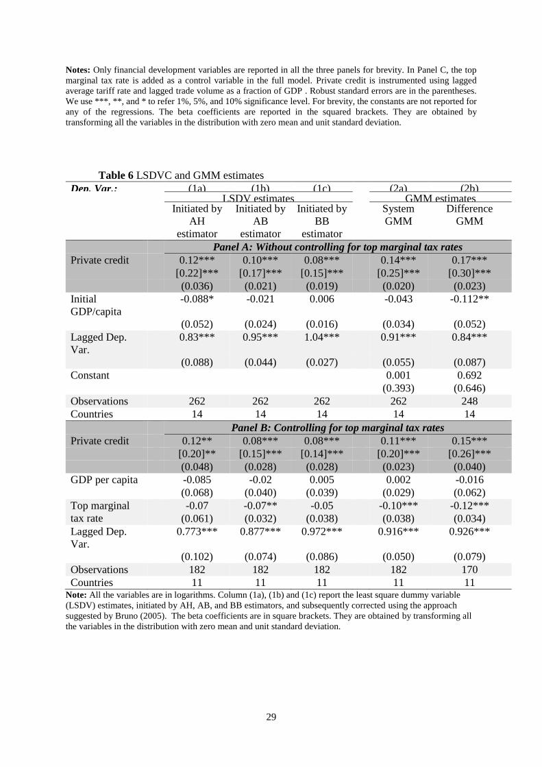
5.5. Robustness check with LSDVC and GMM estimates

Table 6 presents results with corrected least square dummy variable (LSDVC) and

(GMM), controlling for initial GDP per capita in Panel A and GDP per capita, as well as top

marginal tax rates, in Panel B. Columns (1a), (1b) and (1c) report estimates using the LSDVC

technique, initiated via the AH, AB and BB estimators, respectively. The LSDVC technique is

efficient with a narrow, unbalanced panel with long time series, as in our case. The coefficient

16

on FD is significant at the 1% level. However, the estimates are very low in comparison with

the instrumental variable regressions. This may be due to the inclusion of a lagged dependent

variable to capture the dynamicity of the model.

System and difference GMM techniques have the advantage of addressing the feedback

effect on the part of the dependent variable on the explanatory variables using internal

instruments. The results are in Columns (2a) and (2b). The coefficient on private credit is

positive and significant at the 1% level. The size of this coefficient is much larger than the

LSDVC estimates and is similar in magnitude to the OLS results.

The above discussions are based on Panel A, in which we only control for GDP per

capita. Irrespective of the methods applied, we find that financial development has a significant

positive impact on the top 1% of income shares. In Panel B, the top marginal tax rate is included

as an additional control variable to examine the impact of the top marginal tax rate in dynamic

models. The results show that our coefficient of interest remains positive and significant and is

slightly lower than the coefficient obtained in Panel A. The impact of the top marginal tax rate

on top income shares is always negative, as expected; however, in the presence of the financial

development variable, the impact of tax policy is not always significant.

5.6. Robustness check using error-correction models

The LSDVC estimator requires the explanatory variables to be strictly exogenous. We,

therefore, estimate the financial development and top income relationship with other dynamic

models to compare the results. Table 7 reports the results of the mean group estimations (MG),

pooled mean group estimation (PMG) and dynamic fixed-effect estimation (DFE) through error

correction in the long term. All the variables included in the regressions are I(1). The results in

Table 6 confirm a long-term relationship between private credit and the top 1% of income

shares. The adjustment terms (∅𝑖) that characterise the error-correction speed are significant at

the 1% level across the estimators with an expected negative sign. Across the estimates, private

17

credit has a positive impact, and GDP per capita has a negative impact on the top 1% of income

shares. However, the impacts are highly significant only in the PMG and DFE estimates. The

Hausman test between the groups suggests that DFE is the most efficient estimator of the three.

The DFE results show that a 1% increase in private credit is associated with an increase

in the top 1% of income shares of 0.75%, which is very close to our benchmark result (0.7%)

in Table 2. The DFE estimates, thus, reconfirm the contribution of financial development to

enhancing the top income shares in our benchmark results in Table 2.

5.7. Non parametric estimates

Given that the data spans a period of nearly 110 years, one may be concerned that the

point estimates obtained from OLS and IV regressions are not capable of fully capturing the

nature of the relationship between financial development and the top income shares in our

sample. In order to address this limitation associated with point estimates, and to fully capture

the complex nature of the relationship between the financial development and the top income

shares, we use a non-parametric model to further study this relationship. The non-parametric

model can be specified as follows (Silvapulle at al., 2017; Hailemariam at al., 2018):

ln(𝑇𝑂𝑃𝑖𝑡) = 𝑓𝑖(𝑡) + 𝛽1(t) ln(𝐹𝐷𝑖𝑡) + 𝛽2(t) ln(𝐺𝐷𝑃𝑖𝑡) + 𝛽3(t) ln(𝐼𝑛𝑣𝑖𝑡) + 𝛽4(t) ln(𝑆𝑎𝑣𝑖𝑡)+ 𝛽5(𝑡) ln(𝑅𝐷𝐼𝑖𝑡) + 𝛽6(𝑡) ln(𝐸𝐷𝑈𝑖𝑡) + 𝛽7(𝑡) ln(𝑇𝑒𝑟𝑡𝑖𝑡) + 𝛽8(t) ln(𝐺𝐸𝑖𝑡)+ 𝑢𝑖𝑡

In the above equation 𝑓𝑖(𝑡) = 𝑓𝑖 (𝑡

𝑇), for 𝑖 = 1,2, … . , 𝑁 are individual trend functions

for each country in the sample, 𝛽𝑖(𝑡) = 𝛽𝑖 (𝑡

𝑇) are the time-varying coefficients. 𝐹𝐷𝑖𝑡

represents financial development as measured by private credit as a percentage of GDP,

𝐺𝐷𝑃𝑖𝑡 is initial GDP per capita, 𝐼𝑛𝑣𝑖𝑡 is Investment, 𝑆𝑎𝑣𝑖𝑡is Savings, 𝑅𝐷𝐼𝑖𝑡 is R&D intensity,

𝐸𝐷𝑈𝑖𝑡 and 𝑇𝑒𝑟𝑡𝑖𝑡 are average years of education and the percentage of population with

tertiary educational qualifications respectively and 𝐺𝐸𝑖𝑡 is government expenditure.

This specification can be estimated using local linear dummy variable estimation

(LLDVE), following an approach similar to Silvapulle at al. (2017) and Hailemariam at al

18

(2018). We use the leave-one-unit-out least square validation method outlined in Silvapulle at

al. (2017) to select the bandwidth for LLDVE and employ a wild bootstrap procedure to

compute the time confidence intervals for the common trend and coefficient functions. The

LLDVE results are presented in Figure 2. The findings suggest that the relationship between

private credit and top income share is indeed non-linear. But, apart from a period in the 1920s

and 1930s, around the Great Depression, in which the relationship is insignificant, private

credit is positive throughout the twentieth century. Thus, the non-parametric estimates in

Figure 2 are consistent with our parametric point estimates presented in Table 2.

6. Conclusions

Although top incomes have received increased attention in the last few years, we know

very little about the effect of FD on top income shares. Our study has been the first to focus on

the relationship between FD and top incomes by using an instrumental variable approach to

exploit the causal impact of FD on top income shares. We find that irrespective of the measures

used for financial development and top income shares, financial development increases top

income shares. Specifically, we have found that a one-standard-deviation increase in private

credit (as a percentage of GDP) is associated with around a one-standard-deviation increase in

the top 1% of income shares. We also found that the most affluent are the biggest beneficiaries

of financial development.; in particular the top 1% income group derives more benefits from

financial development than the top 5%, and the top 5% derives more benefit than the top 10%.

Another significant finding of our work is that the shares of the top income groups

remain partly balanced because the impact of financial and economic development affect top

income shares in opposite directions. While financial development contributes to increasing

top income shares, economic development reduces them. Thus, economic development

(increasing income per capita) remains crucial for OECD countries in that it can dampen the

aggressive and positive impact of financial development on top income shares. Interestingly,

we do not find that top marginal tax rates have any significant effect on top income shares. In

19

contrast, rising tertiary education and R&D expenditures boost the incomes of the rich. The

results substantiate Piketty’s (2014) worries regarding the increasing gap between the rich and

the poor because advances in both technology and higher education ultimately favour the rich,

allowing them to consolidate their wealth, given that they are the primary beneficiaries of

capital returns and are the leading employers of the highly educated workforce.

20

References Acemoglu, D., Robinson, J.A., 2000. Political Losers as a Barrier to Economic Development. The

American Economic Review 90, 126-130

Acemoglu, D., Johnson, S., Robinson, J.A., 2001. The Colonial Origins of Comparative Development:

An Empirical Investigation. American Economic Review 91, 1369-1401

Alesina, A., and Roberto Perotti. 1996. Income distribution, political instability, and investment.

European Economic Review 40(6): 1203-1228.

Alvaredo, F., Atkinson, A.B., Piketty, T., Saez, E., 2013. The Top 1 Percent in International and

Historical Perspective. Journal of Economic Perspectives 27, 3-20

Andrews, D., Jencks, C., & Leigh, A. (2011). Do Rising Top Incomes Lift All Boats ? The B . E .

Journal of Economic Analysis & Policy, 11(1).

Arcand, J.L., Berkes, E., Panizza, U., 2015. Too much finance? Journal of Economic Growth 20, 105-

148

Atkinson, A.B., 2004. Income tax and top incomes over the twentieth century. Revista de Economia

Publica 168, 123-141

Atkinson, A.B., 2005. Comparing the Distribution of Top Incomes across Countries. Journal of the

European Economic Association 3, 393-401

Atkinson, A.B., Leigh, A., 2013. The Distribution of Top Incomes in Five Anglo-Saxon Countries Over

the Long Run. Economic Record 89, 31-47

Atkinson, A.B., Piketty, T., Saez, E., 2011. Top Incomes in the Long Run of History. Journal of

Economic Literature 49, 3-71

Atkinson, A.B., Søgaard, J.E., 2013. The long-run history of income inequality in Denmark: Top

incomes from 1870 to 2010. In: EPRU Working Paper Series, 2013-0.

Baltagi, B.H., P.O. Demetriades and S.H. Law (2009). Financial Development and Openness: Evidence

from Panel Data. Journal of Development Economics, 89(2), 285-296

Banerjee, A.V., Newman, A.F., 1993. Occupational Choice and the Process of Development. Journal

of Political Economy 101, 274-298

Beck, T., Demirgüç-Kunt, A., Levine, R., 2007. Finance, inequality and the poor. Journal of Economic

Growth 12, 27-49

Beck, T., Levine, R., 2004. Stock markets, banks, and growth: Panel evidence. Journal of Banking &

Finance 28, 423-442.

Bordo, M.D., Meissner, C.M. (2012). Does inequality lead to a financial crisis? Journal of International

Money and Finance, 31, 2147-2161.

Bruno, G.S.F., 2005. Estimation and inference in dynamic unbalanced panel-data models with a small

number of individuals. The Stata Journal 5, 473-500

Chambers, D., 2007. Trading places: Does past growth impact inequality? Journal of Development

Economics 82, 257-266.

21

Chinn, M.D. and H. Ito (2006). What Matters for Financial Development? Capital Controls, Institutions,

and Interactions. Journal of Development Economics, 81 (1), 163-192.

Clarke, G.R.G., Lixin Colin, X., Heng-Fu, Z., 2006. Finance and Income Inequality: What Do the Data

Tell Us? Southern Economic Journal 72, 578-596

De Bonis R. and M. Stacchini (2009) What Determines the Size of Bank Loans in Industrialized

Countries? The Role of Government Debt. Bank of Italy Working Paper 707, Banca d'Italia,

Rome.

de Haan, J. and J-E. Sturm (2017). Finance and Income Inequality: A Review and New Evidence.

European Journal of Political Economy, 50, 171- 195.

Dollar, D., Kleineberg, T., Kraay, A., 2013. Growth still is good for the poor. URL

http://elibrary.worldbank.org/doi/pdf/10.1596/1813-9450-6568

Dollar, D., Kraay, A., 2002. Growth Is Good for the Poor. Journal of Economic Growth 7, 195-225

Dumitrescu, E.-I., Hurlin, C., 2012. Testing for Granger non-causality in heterogeneous panels.

Economic Modelling 29, 1450-1460

Galor, O., Zeira, J., 1993. Income Distribution and Macroeconomics. Review of Economic Studies 60,

35-52.

Greenwood, J., Jovanovic, B., 1990. Financial Development, Growth, and the Distribution of Income.

Journal of Political Economy 98, 1076-1107.

Hailemariam, A., Smyth, R. & Zhang, X. (2018). Oil prices and economic policy umncertainty:

Evidence from a nonparametric panel data model. Unpublished manuscript, Department of

Economics, Monash University.

Huang, Y., Temple, J., 2005. Does external trade promote financial development? Federal Reserve

Bank of St Louis, St. Louis

Ilyina, A., Samaniego, R., 2011. Technology and Financial Development. Journal of Money, Credit and

Banking 43, 899-921

Jerzmanowski, M., Nabar, M., 2013. Financial development and wage inequality: Theory and evidence.

Economic Inquiry 51, 211-234

King, R.G., Levine, R., 1993. Finance and growth: Schumpeter might be right. Quarterly Journal of

Economics 108, 717.

Kumhof, M., Rancière, R., Winant, P. (2015). Inequality, leverage and crises. American Economic

Review, 105, 1217-1245

Kuznets, S., 1955. Economic growth and income inequality. American Economic Review 45, 1

Lopez, H., 2006. Growth and inequality: Are the 1990s different? Economics Letters 93, 18-25

Madsen, J. B. 2010. The anatomy of growth in the OECD since 1870. Journal of Monetary Economics,

57(6), 753–767.

22

Madsen, J. B. 2014. Human capital and the world technology frontier. Review of Economics and

Statistics, 96(4), 676-692.

Madsen, J.B., Ang, J.B., 2016. Finance-Led Growth in the OECD since the Nineteenth Century: How

Does Financial Development Transmit to Growth? Review of Economics and Statistics 98,

552-572

Madsen, J.B., Islam, M. R., & Doucouliagos, H. (2018). Inequality, financial development and

economic growth in the OECD, 1870-2011. European Economic Review, 101.

Moriguchi, C., 2010. Top wage incomes in Japan, 1951–2005. Journal of the Japanese and International

Economies 24, 301-333.

Philippe, A., Eve, C., Cecilia, G.-P., 1999. Inequality and economic growth: The perspective of the new

growth theories. Journal of Economic Literature 37, 1615-1660

Piketty, T., 2001. Income inequality in France, 1900-1998. In: CEPR Discussion Papers, No. 2876

Piketty, T., 2014. Capital in the Twenty-First Century. Harvard University Press.

Quy-Toan, D., Levchenko, A.A., 2004. Trade and financial development. In: Policy Research Working

Paper. World Bank, Washington DC

Rajan, R.G., Zingales, L., 2003. The great reversals: the politics of financial development in the

twentieth century. Journal of Financial Economics 69, 5-50

Roine, J., Vlachos, J., Waldenström, D., 2009. The long-run determinants of inequality: What can we

learn from top income data? Journal of Public Economics 93, 974-988

Saez, E., 2005. Top Incomes in the United States and Canada Over the Twentieth Century. Journal of

the European Economic Association 3, 402-411

Saez, E., 2017. Income and Wealth inequality. Evidence and Policy Implications. Contemporary

Economic Policy 35, 7-25.

Silvapulle, P., Smyth, R., Zhang, X. & Fenech, J.P. (2017). Nonparametric panel data model for crude

oil and stock market prices in net oil importing countries. Energy Economics 67, 255-267

Staiger, D., Stock, J.H., 1997. Instrumental Variables Regression with Weak Instruments. Econometrica

65, 557-586.

Stulz, R. and R. Williamson (2003). Culture, Openness, and Finance. Journal of Financial Economics,

70, 313-349

Tanndal, J., & Waldenström, D. (2018). Does Financial Deregulation Boost Top Incomes? Evidence

from the Big Bang. Economica, 85(338), 232–265.

Veall, M.R., 2012. Top income shares in Canada: recent trends and policy implications. Portion des

plus hauts revenus au Canada: tendances récentes et implications pour les politiques . Canadian

Journal of Economics 45, 1247-1272.

World Bank (2018). The Changing Wealth of Nations 2018: Building a Sustainable Future (World Bank:

Washington DC).

23

24

Tables and Figures

Table 1 Description of variables and data sources

Note: All the variables are expressed in natural logarithm. Professor Jakob Madsen shared the tariff data.

5 Export data is not available for many countries in the early decades of the last century. Hence, Import-

GDP ratio is used as a proxy for openness.

Variable Description Source

Top income

shares

Data are downloaded from World Top Income Database

of Paris School of Economics. They are before tax data

and are expressed as a percentage of GDP. The data are

derived from the tax returns of the countries.

World Wealth and

Income Database

(wid.world)

Private credit Credit to private sector as percentage of GDP Madsen and Ang

(2016)

Bank assets Bank assets as a percentage of GDP Madsen and Ang

(2016)

Broad Money Broad money includes currency, other liquid assets as

well as long-term investment in bonds and other liquid

assets

Madsen and Ang

(2016)

GDP per capita GDP per capita is measured in 1990 International

Geary-Khamis dollars from the Maddison Project

Database.

http://www.ggdc.net

Trade

openness Imports as the percentage of GDP5 Madsen and Ang

(2016)

Tariff rate Nominal import duties as a percentage of nominal

import values of goods

Madsen (2010)

Agriculture

share

Agriculture share in income as the share of agricultural

production in total GDP

Madsen and Ang

(2016)

Educational

attainment

Educational attainment in average years of education Madsen (2014)

Tertiary

education

Fraction of the population in the 18- to 22-year-age

cohort enrolled in tertiary education

Madsen and Ang

(2016)

Investment Investment as a percentage of total capital stock Madsen and Ang

(2016)

Government

expenditure

Government expenditure as a percentage of GDP Roine et al. (2009)

Top marginal

tax rates

These are statutory top tax rates of a country. For UK

and USA, we use the tax rates applicable to incomes

higher than five times GDP per capita, following Roine

et al. (2009)

Roine et al. (2009)

R&D intensity Research and development expenditure as % of GDP. Madsen and Ang

(2016)

25

Table 2 Effect of Financial development on top 1% income shares (1) (2) (3) (4) (5)

Dep. Var.= Top 1%

income shares (ln) OLS OLS IV1+IV2 IV1+IV3 IV1+IV2+IV3

Panel A: 2SLS results

Private credit -0.029 0.187*** 0.629*** 0.701*** 0.633***

[Beta coefficient] [-0.05] [0.30]*** [1.1]*** [1.2]*** [1.1]*** (0.036) (0.029) (0.089) (0.096) (0.088)

Initial GDP per capita

-0.448*** -0.714*** -0.750*** -0.725***

[Beta coefficient] [-0.78]*** [-1.25]*** [-1.31]*** [-1.25]*** (0.029) (0.045) (0.047) (0.043)

Hansen Chi2 p-value 0.553 0.839 0.139

Observations 240 240 240 240 240

Countries 14 14 14 14 14

R-squared 0.002 0.477 0.552 0.495 0.550

Panel B: First stage results

Trade openness

0.373*** 0.423*** 0.366*** (0.061) (0.059) (0.069)

Tariff rate

-0.977**

-0.914** (0.427)

(0.425)

Agriculture share

-0.139 -0.093 (0.109) (0.107)

Initial GDP per capita

0.360*** 0.250* 0.253** (0.043) (0.129) (0.127)

Observations

240 240 240

First stage F-stat (excl.

IV)

26.7 27.1 18.1

First stage partial R2

0.194 0.175 0.197

First stage R2

0.517 0.506 0.512 Notes: Private credit is instrumented using the followings: lagged trade volume as a fraction of GDP (IV1),

lagged average tariff rate (IV2), and agriculture share in income (IV3). Robust standard errors are in parentheses.

We use ***, **, and * to refer 1%, 5%, and 10% significance level. For brevity, the constants are not reported for

any of the regressions. The beta coefficients are reported in the squared brackets. They are obtained by

transforming all the variables in the distribution with zero mean and unit standard deviation.

26

Table 3 Full model of FD and Top 1% Income shares

(1) (2) (3) (4)

Dep. Var.=Top 1% income share OLS IV regressions

Private credit 0.151*** 0.140*** 0.700*** 0.603***

[0.23]*** [0.22]*** [1.08]*** [0.96]*** (0.032) (0.034) (0.161) (0.163)

Initial GDP per capita -0.239** -0.309*** -0.855*** -0.587***

[-0.41]*** [-0.50]*** [-1.48]*** [-0.95]*** (0.093) (0.095) (0.180) (0.158)

Investment 0.225 0.298* -0.154 0.007 (0.138) (0.157) (0.159) (0.164)

Saving -0.379*** -0.584*** 0.05 -0.209 (0.099) (0.105) (0.106) (0.137)

R&D intensity 0.099*** 0.136*** 0.158** 0.174** (0.029) (0.030) (0.066) (0.068)

Years of education 0.098 0.335* -0.255 -0.926*** (0.115) (0.187) (0.162) (0.291)

Fraction of population with Tertiary

education

0.002 -0.001 0.008*** 0.008***

(0.002) (0.002) (0.002) (0.002)

Government expenditure -0.401*** -0.190*** -0.09 -0.246*** (0.065) (0.069) (0.094) (0.063)

Top marginal tax rate

-0.270***

0.075 (0.056)

(0.085)

Hansen J statistics

0.321 0.360

Observations 186 134 186 134

R-squared 0.648 0.684 0.66 0.788

First stage statistics

F-statistic 8.02 6.27

Partial R2 0.132 0.133

R2 0.719 0.796 Notes: lagged trade volume as a fraction of GDP (IV1), lagged average tariff rate (IV2), and agriculture share in

income (IV3). Robust standard errors are in the parentheses. We use ***, **, and * to refer 1%, 5%, and 10%

significance level. The constants are not reported for any of the regressions. The beta coefficients are reported in

the squared brackets. They are obtained by transforming all the variables in the distribution with zero mean and

unit standard deviation.

27

Table 4 Exclusion restriction test-full model

Dep. Var.=Top 1% income shares (1) (2) (3) (4)

Private credit 0.648*** 0.563*** 0.683*** 0.640*** (0.153) (0.158) (0.166) (0.209)

Initial GDP per capita -0.831*** -0.602*** -0.840*** -0.617*** (0.174) (0.150) (0.179) (0.183)

Trade openness 0.095 0.097

(0.061) (0.083)

Tariff rate

-0.008 0.008 (0.017) (0.024)

Top marginal tax rate (TMTR)

0.073

0.090 (0.082)

(0.098)

Observations 186 134 186 134 R-squared 0.685 0.799 0.667 0.778 Hansen J statistic 0.990 0.360 0.185 0.188

First stage statistics

F-statistic 11.9 8.52 11.5 5.68 Partial R2 0.126 0.128 0.124 0.100 R2 0.719 0.796 0.719 0.796

Notes: Trade volume as a fraction of GDP and tariff rates are used as additional control variables in the full

model. All the control variables are not reported to conserve space. The beta coefficients are reported in the

squared brackets. They are obtained by transforming all the variables in the distribution with zero mean and unit

standard deviation. Instruments used for FD are lagged trade volume as a fraction of GDP (IV1), lagged average

tariff rate (IV2), and agriculture share in income (IV3). Robust standard errors are in the parentheses. We use

***, **, and * to refer 1%, 5%, and 10% significance level.

28

Table 5 Robustness check using alternative measures of top income and financial development (1) (2) (3) (4) (5) (6) (7)

Dep. Var.

Top 10% Top 5% Top 0.5% Top 0.1% Top2-

10%

Top 1% Top 1%

Panel A: Basic model

Private credit 0.237*** 0.349**

*

0.719*** 1.185*** 0.045*

[0.92]*** [1.02]**

*

[1.09]**

*

[1.31]*** [0.25]* (0.028) (0.049) (0.090) (0.150) (0.023)

Bank assets

0.839***

[1.37]**

*

(0.193)

Broad money

1.256*** [1.53]***

(0.351) Observations 181 222 188 206 183 240 240 R-squared 0.610 0.539 0.564 0.384 0.213 0.182 -0.115 Hansen J statistic 0.971 0.324 0.047 0.443 0.435 0.308 0.071 First stage F-stat 20.4 18.5 17.8 18.5 19.9 7.87 4.80 Partial R2 0.260 0.191 0.230 0.207 0.253 0.136 0.066 R2 0.477 0.497 0.486 0.496 0.354 0.580 0.181 Panel B: Full model

Private credit 0.248*** 0.424**

*

0.918*** 1.318*** 0.117**

[0.84]*** [1.13]**

*

[1.24]*** [1.31]*** [0.58]** (0.062) (0.077) (0.205) (0.282) (0.055)

Bank assets

0.791***

[1.25]**

*

(0.298)

Broad money

0.722*** [0.79]***

(0.171) Observations 134 170 140 156 135 186 186 R-squared 0.767 0.66 0.628 0.569 0.382 0.404 0.591 Hansen J statistic 0.458 0.143 0.121 0.294 0.008 0.153 0.861 First stage F-stat 7.00 8.54 7.60 8.56 8.31 3.95 7.50 Partial R2 0.110 0.143 0.143 0.146 0.125 0.058 0.136 R2 0.732 0.717 0.700 0.713 0.741 0.735 0.308 Panel C: Full model including top marginal tax rate

Private credit 0.267*** 0.404**

*

0.735*** 0.999*** 0.141*

[0.97]*** [1.11]**

*

[1.04]*** [1.05]*** [0.71]* (0.086) (0.098) (0.248) (0.269) (0.080)

Bank assets

0.716**

[1.11]** (0.297)

Broad money

0.426*** [0.48]***

(0.119) Top marginal tax

rate

0.088** 0.04 0.13 0.162 0.053 0.014 -0.128** (0.035) (0.056) (0.131) (0.141) (0.036) (0.098) (0.052)

Observations 108 134 117 129 109 134 134 R-squared 0.747 0.703 0.794 0.776 0.384 0.695 0.799 Hansen J statistic 0.998 0.070 0.103 0.230 0.191 0.069 0.006 First stage F-stat 4.34 6.30 4.10 6.40 5.10 2.05 5.6 Partial R2 0.105 0.133 0.120 0.140 0.116 0.069 0.127 R2 0.800 0.796 0.793 0.798 0.810 0.818 0.518

29

Notes: Only financial development variables are reported in all the three panels for brevity. In Panel C, the top

marginal tax rate is added as a control variable in the full model. Private credit is instrumented using lagged

average tariff rate and lagged trade volume as a fraction of GDP . Robust standard errors are in the parentheses.

We use ***, **, and * to refer 1%, 5%, and 10% significance level. For brevity, the constants are not reported for

any of the regressions. The beta coefficients are reported in the squared brackets. They are obtained by

transforming all the variables in the distribution with zero mean and unit standard deviation.

Table 6 LSDVC and GMM estimates

Dep. Var.:

TOP1%

(1a) (1b) (1c) (2a) (2b) LSDV estimates GMM estimates Initiated by

AH

estimator

Initiated by

AB

estimator

Initiated by

BB

estimator

System

GMM

Difference

GMM

Panel A: Without controlling for top marginal tax rates

Private credit 0.12*** 0.10*** 0.08*** 0.14*** 0.17***

[0.22]*** [0.17]*** [0.15]*** [0.25]*** [0.30]*** (0.036) (0.021) (0.019) (0.020) (0.023)

Initial

GDP/capita

-0.088* -0.021 0.006 -0.043 -0.112**

(0.052) (0.024) (0.016) (0.034) (0.052)

Lagged Dep.

Var.

0.83*** 0.95*** 1.04*** 0.91*** 0.84***

(0.088) (0.044) (0.027) (0.055) (0.087)

Constant

0.001 0.692

(0.393) (0.646)

Observations 262 262 262 262 248

Countries 14 14 14 14 14

Panel B: Controlling for top marginal tax rates

Private credit 0.12** 0.08*** 0.08*** 0.11*** 0.15***

[0.20]** [0.15]*** [0.14]*** [0.20]*** [0.26]*** (0.048) (0.028) (0.028) (0.023) (0.040)

GDP per capita -0.085 -0.02 0.005 0.002 -0.016 (0.068) (0.040) (0.039) (0.029) (0.062)

Top marginal

tax rate

-0.07 -0.07** -0.05 -0.10*** -0.12***

(0.061) (0.032) (0.038) (0.038) (0.034)

Lagged Dep.

Var.

0.773*** 0.877*** 0.972*** 0.916*** 0.926***

(0.102) (0.074) (0.086) (0.050) (0.079)

Observations 182 182 182 182 170

Countries 11 11 11 11 11 Note: All the variables are in logarithms. Column (1a), (1b) and (1c) report the least square dummy variable

(LSDV) estimates, initiated by AH, AB, and BB estimators, and subsequently corrected using the approach

suggested by Bruno (2005). The beta coefficients are in square brackets. They are obtained by transforming all

the variables in the distribution with zero mean and unit standard deviation.

30

Table 7 Error correction models’ estimates

Mean group

(MG)

Pooled Mean Group

(PMG)

Dynamic Fixed Effect

(DFE) (1a)

LR

(1b)

SR

(2a)

LR

(2b)

SR

(3a)

LR

(3b)

SR Dep. Var.: Top 1% income shares

Private credit 0.262

1.240***

0.749***

(0.638)

(0.258)

(0.179)

GDP per capita -2.145

-0.484***

-

0.511***

(1.681)

(0.074)

(0.086)

Error correction

(∅𝑖)

-0.281***

-0.132***

-0.182***

(0.101)

(0.036)

(0.045)

∆Private credit

-0.018

-0.025

-0.025 (0.061)

(0.063)

(0.046)

∆GDP per capita

0.084

0.072

0.103 (0.118)

(0.123)

(0.119)

Constant

1.560**

0.178***

0.680** (0.714)

(0.051)

(0.303)

Observations 262 262 262 262 248 248 Note: All the variables are in logarithms. Im-Pesaran-Shin panel unit-root tests indicate that all the main variables-

private credit, top 1% income shares, and GDP per capita are I(1). Non-zero, negative ∅i confirms a long run

relationship between private credit and top 1% income shares at 1% level of significance. Comparison among the

estimators using the Hausman test suggests that DFE estimates are preferable.

31

Figures

Figure 1 Log-log plot of Ppivate credit and external instruments

2.5

33.

54

4.5

5

Priv

ate

cred

it

1 2 3 4 5One period lag of Openness

2.5

33.

54

4.5

5

Priv

ate

cred

it

-5 -4 -3 -2 -1 0One period lag of tariff rate

2.5

33.

54

4.5

5

Priv

ate

cred

it

-5 -4 -3 -2 -1 0Agriculture share in GDP

AUS CAN NZL GBR USA DNK FIN

NOR SWE FRA DEU JPN NLD CHE

32

Figure 2. Non-Parametric local linear estimates

33

34

Online Appendix

Table A1 Summary of key variables

Variables Observatio

n

Mean St. dev. Min Max

Private credit 308 3.942 0.722 2.427 5.367

GDP per capita 308 8.905 0.730 7.072 10.260

Trade openness 253 3.527 0.727 -0.876 5.903

Investment 462 -2.244 0.239 -3.572 -1.715

Broad money 462 -0.407 0.694 -3.533 1.527

Saving 305 -1.740 0.418 -3.869 -1.022

Tariff rate 294 -2.821 1.281 -11.243 -0.118

Agriculture share 462 -2.405 1.008 -5.055 -0.322

R&D intensity 308 -4.411 0.889 -7.594 -2.832

Education years 308 2.126 0.377 -0.163 2.721

Bank assets 308 4.311 0.656 2.920 6.293

Government

expenditure

279 -2.133 0.607 -4.506 -0.876

R&D intensity 308 -4.410 0.889 -7.593 -2.831

Top marginal tax rates 196 -0.858 0.637 -3.689 -0.025

Top 10% income

shares

216 3.532 0.179 3.095 4.099

Top 5% income shares 266 3.157 0.236 2.572 3.720

Top 1% income shares 288 2.310 0.407 1.348 3.285

Top 0.5% income

shares

225 1.971 0.472 0.801 3.019

Top 0.1% income

shares

247 1.150 0.634 -0.572 2.589

Note: Variables are in natural logarithms

Table A2 Correlation among key variables (1) (2) (3) (4) (5) (6) (7) (8) (9)

(1)Top1 1

(2)GDP per capita -

0.60

1

(3) Private credit -

0.06

0.50 1

(4)Tariff rate 0.35 -

0.55

-0.43 1

(5)Openness -

0.16

0.27 0.10 -

0.48

1

(6)Educational

attainment

-

0.37

0.77 0.36 -

0.38

-

0.03

1

(7) Bank assets -

0.23

0.58 0.74 -

0.54

0.35 0.36 1

(8)Govt. expenditure -

0.68

0.72 0.21 -

0.51

0.21 0.48 0.38 1

(9) R&D intensity -

0.36

0.56 0.21 -

0.25

-

0.03

0.40 0.28 0.57 1

35

Note: Variables are in natural logarithm