financial derivatives toolbox - department of radio...
TRANSCRIPT

Computation
Visualization
Programming
For Use with MATLAB®
User’s GuideVersion 1
Financial DerivativesToolbox

How to Contact The MathWorks:
508-647-7000 Phone
508-647-7001 Fax
The MathWorks, Inc. Mail3 Apple Hill DriveNatick, MA 01760-2098
http://www.mathworks.com Webftp.mathworks.com Anonymous FTP servercomp.soft-sys.matlab Newsgroup
[email protected] Technical [email protected] Product enhancement [email protected] Bug [email protected] Documentation error [email protected] Subscribing user [email protected] Order status, license renewals, [email protected] Sales, pricing, and general information
Financial Derivatives Toolbox User’s Guide COPYRIGHT 2000 by The MathWorks, Inc.The software described in this document is furnished under a license agreement. The software may be usedor copied only under the terms of the license agreement. No part of this manual may be photocopied or repro-duced in any form without prior written consent from The MathWorks, Inc.
FEDERAL ACQUISITION: This provision applies to all acquisitions of the Program and Documentation byor for the federal government of the United States. By accepting delivery of the Program, the governmenthereby agrees that this software qualifies as "commercial" computer software within the meaning of FARPart 12.212, DFARS Part 227.7202-1, DFARS Part 227.7202-3, DFARS Part 252.227-7013, and DFARS Part252.227-7014. The terms and conditions of The MathWorks, Inc. Software License Agreement shall pertainto the government’s use and disclosure of the Program and Documentation, and shall supersede anyconflicting contractual terms or conditions. If this license fails to meet the government’s minimum needs oris inconsistent in any respect with federal procurement law, the government agrees to return the Programand Documentation, unused, to MathWorks.
MATLAB, Simulink, Stateflow, Handle Graphics, and Real-Time Workshop are registered trademarks, andTarget Language Compiler is a trademark of The MathWorks, Inc.
Other product or brand names are trademarks or registered trademarks of their respective holders.
Printing History: June 2000 First printing New for Version 1 (Release 12)

i
Contents
Preface
About this Book . . . . . . . . . . . . . . . . . . . . . . . . . . . . . . . . . . . . . . viiiOrganization of the Document . . . . . . . . . . . . . . . . . . . . . . . . . . viiiTypographical Conventions . . . . . . . . . . . . . . . . . . . . . . . . . . . . viii
Related Products . . . . . . . . . . . . . . . . . . . . . . . . . . . . . . . . . . . . . . . x
Further Reading . . . . . . . . . . . . . . . . . . . . . . . . . . . . . . . . . . . . . . xiiHeath-Jarrow-Morton Modeling . . . . . . . . . . . . . . . . . . . . . . . . . xiiFinancial Derivatives . . . . . . . . . . . . . . . . . . . . . . . . . . . . . . . . . xii
1Tutorial
Introduction . . . . . . . . . . . . . . . . . . . . . . . . . . . . . . . . . . . . . . . . . 1-2Interest Rate Models . . . . . . . . . . . . . . . . . . . . . . . . . . . . . . . . . . 1-2Financial Instruments . . . . . . . . . . . . . . . . . . . . . . . . . . . . . . . . 1-3Hedging . . . . . . . . . . . . . . . . . . . . . . . . . . . . . . . . . . . . . . . . . . . . 1-4
Creating and Managing Instrument Portfolios . . . . . . . . . . 1-5Portfolio Creation . . . . . . . . . . . . . . . . . . . . . . . . . . . . . . . . . . . . 1-5Portfolio Management . . . . . . . . . . . . . . . . . . . . . . . . . . . . . . . . . 1-7
Interest Rate Environment . . . . . . . . . . . . . . . . . . . . . . . . . . . 1-16Interest Rates vs. Discount Factors . . . . . . . . . . . . . . . . . . . . . 1-16Interest Rate Term Conversions . . . . . . . . . . . . . . . . . . . . . . . . 1-21Interest Rate Term Structure . . . . . . . . . . . . . . . . . . . . . . . . . . 1-25
Pricing and Sensitivity from Interest Term Structure . . . 1-30Pricing . . . . . . . . . . . . . . . . . . . . . . . . . . . . . . . . . . . . . . . . . . . . 1-31Sensitivity . . . . . . . . . . . . . . . . . . . . . . . . . . . . . . . . . . . . . . . . . 1-33

ii Contents
Heath-Jarrow-Morton (HJM) Model . . . . . . . . . . . . . . . . . . . 1-35Building an HJM Forward Rate Tree . . . . . . . . . . . . . . . . . . . . 1-35Using HJM Trees in MATLAB . . . . . . . . . . . . . . . . . . . . . . . . . 1-41
Pricing and Sensitivity from HJM . . . . . . . . . . . . . . . . . . . . . 1-48Pricing and the Price Tree . . . . . . . . . . . . . . . . . . . . . . . . . . . . . 1-48Calculating Prices and Sensitivities . . . . . . . . . . . . . . . . . . . . . 1-61
Hedging . . . . . . . . . . . . . . . . . . . . . . . . . . . . . . . . . . . . . . . . . . . . . 1-64Hedging Functions . . . . . . . . . . . . . . . . . . . . . . . . . . . . . . . . . . . 1-64Hedging with hedgeopt . . . . . . . . . . . . . . . . . . . . . . . . . . . . . . . 1-65Self Financing Hedges (hedgeslf) . . . . . . . . . . . . . . . . . . . . . . . 1-72Specifying Constraints with ConSet . . . . . . . . . . . . . . . . . . . . . 1-75Hedging with Constrained Portfolios . . . . . . . . . . . . . . . . . . . . 1-79
2Function Reference
Functions by Category . . . . . . . . . . . . . . . . . . . . . . . . . . . . . . . . 2-2
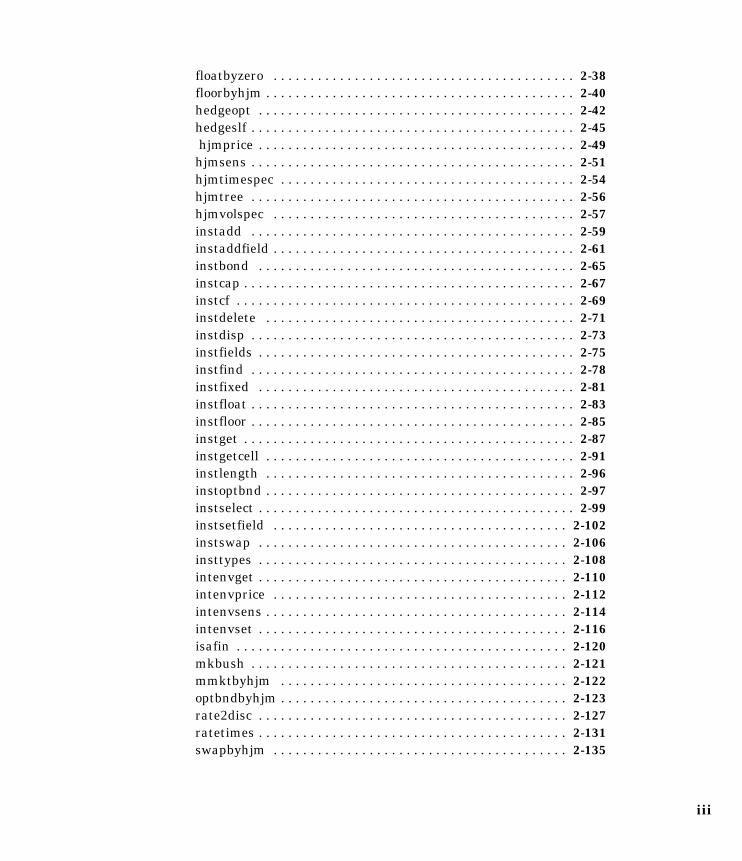
Alphabetical List of Functions . . . . . . . . . . . . . . . . . . . . . . . . . 2-7bondbyhjm . . . . . . . . . . . . . . . . . . . . . . . . . . . . . . . . . . . . . . . . . . 2-9bondbyzero . . . . . . . . . . . . . . . . . . . . . . . . . . . . . . . . . . . . . . . . . 2-12bushpath . . . . . . . . . . . . . . . . . . . . . . . . . . . . . . . . . . . . . . . . . . . 2-15bushshape . . . . . . . . . . . . . . . . . . . . . . . . . . . . . . . . . . . . . . . . . . 2-16capbyhjm . . . . . . . . . . . . . . . . . . . . . . . . . . . . . . . . . . . . . . . . . . . 2-18cfbyhjm . . . . . . . . . . . . . . . . . . . . . . . . . . . . . . . . . . . . . . . . . . . . 2-20 cfbyzero . . . . . . . . . . . . . . . . . . . . . . . . . . . . . . . . . . . . . . . . . . . 2-21classfin . . . . . . . . . . . . . . . . . . . . . . . . . . . . . . . . . . . . . . . . . . . . 2-22date2time . . . . . . . . . . . . . . . . . . . . . . . . . . . . . . . . . . . . . . . . . . 2-24datedisp . . . . . . . . . . . . . . . . . . . . . . . . . . . . . . . . . . . . . . . . . . . 2-26derivget . . . . . . . . . . . . . . . . . . . . . . . . . . . . . . . . . . . . . . . . . . . . 2-27derivset . . . . . . . . . . . . . . . . . . . . . . . . . . . . . . . . . . . . . . . . . . . . 2-28disc2rate . . . . . . . . . . . . . . . . . . . . . . . . . . . . . . . . . . . . . . . . . . . 2-30fixedbyhjm . . . . . . . . . . . . . . . . . . . . . . . . . . . . . . . . . . . . . . . . . 2-32fixedbyzero . . . . . . . . . . . . . . . . . . . . . . . . . . . . . . . . . . . . . . . . . 2-34floatbyhjm . . . . . . . . . . . . . . . . . . . . . . . . . . . . . . . . . . . . . . . . . . 2-36
iii
floatbyzero . . . . . . . . . . . . . . . . . . . . . . . . . . . . . . . . . . . . . . . . . 2-38floorbyhjm . . . . . . . . . . . . . . . . . . . . . . . . . . . . . . . . . . . . . . . . . . 2-40hedgeopt . . . . . . . . . . . . . . . . . . . . . . . . . . . . . . . . . . . . . . . . . . . 2-42hedgeslf . . . . . . . . . . . . . . . . . . . . . . . . . . . . . . . . . . . . . . . . . . . . 2-45 hjmprice . . . . . . . . . . . . . . . . . . . . . . . . . . . . . . . . . . . . . . . . . . . 2-49hjmsens . . . . . . . . . . . . . . . . . . . . . . . . . . . . . . . . . . . . . . . . . . . . 2-51hjmtimespec . . . . . . . . . . . . . . . . . . . . . . . . . . . . . . . . . . . . . . . . 2-54hjmtree . . . . . . . . . . . . . . . . . . . . . . . . . . . . . . . . . . . . . . . . . . . . 2-56hjmvolspec . . . . . . . . . . . . . . . . . . . . . . . . . . . . . . . . . . . . . . . . . 2-57instadd . . . . . . . . . . . . . . . . . . . . . . . . . . . . . . . . . . . . . . . . . . . . 2-59instaddfield . . . . . . . . . . . . . . . . . . . . . . . . . . . . . . . . . . . . . . . . . 2-61instbond . . . . . . . . . . . . . . . . . . . . . . . . . . . . . . . . . . . . . . . . . . . 2-65instcap . . . . . . . . . . . . . . . . . . . . . . . . . . . . . . . . . . . . . . . . . . . . . 2-67instcf . . . . . . . . . . . . . . . . . . . . . . . . . . . . . . . . . . . . . . . . . . . . . . 2-69instdelete . . . . . . . . . . . . . . . . . . . . . . . . . . . . . . . . . . . . . . . . . . 2-71instdisp . . . . . . . . . . . . . . . . . . . . . . . . . . . . . . . . . . . . . . . . . . . . 2-73instfields . . . . . . . . . . . . . . . . . . . . . . . . . . . . . . . . . . . . . . . . . . . 2-75instfind . . . . . . . . . . . . . . . . . . . . . . . . . . . . . . . . . . . . . . . . . . . . 2-78instfixed . . . . . . . . . . . . . . . . . . . . . . . . . . . . . . . . . . . . . . . . . . . 2-81instfloat . . . . . . . . . . . . . . . . . . . . . . . . . . . . . . . . . . . . . . . . . . . . 2-83instfloor . . . . . . . . . . . . . . . . . . . . . . . . . . . . . . . . . . . . . . . . . . . . 2-85instget . . . . . . . . . . . . . . . . . . . . . . . . . . . . . . . . . . . . . . . . . . . . . 2-87instgetcell . . . . . . . . . . . . . . . . . . . . . . . . . . . . . . . . . . . . . . . . . . 2-91instlength . . . . . . . . . . . . . . . . . . . . . . . . . . . . . . . . . . . . . . . . . . 2-96instoptbnd . . . . . . . . . . . . . . . . . . . . . . . . . . . . . . . . . . . . . . . . . . 2-97instselect . . . . . . . . . . . . . . . . . . . . . . . . . . . . . . . . . . . . . . . . . . . 2-99instsetfield . . . . . . . . . . . . . . . . . . . . . . . . . . . . . . . . . . . . . . . . 2-102instswap . . . . . . . . . . . . . . . . . . . . . . . . . . . . . . . . . . . . . . . . . . 2-106insttypes . . . . . . . . . . . . . . . . . . . . . . . . . . . . . . . . . . . . . . . . . . 2-108intenvget . . . . . . . . . . . . . . . . . . . . . . . . . . . . . . . . . . . . . . . . . . 2-110intenvprice . . . . . . . . . . . . . . . . . . . . . . . . . . . . . . . . . . . . . . . . 2-112intenvsens . . . . . . . . . . . . . . . . . . . . . . . . . . . . . . . . . . . . . . . . . 2-114intenvset . . . . . . . . . . . . . . . . . . . . . . . . . . . . . . . . . . . . . . . . . . 2-116isafin . . . . . . . . . . . . . . . . . . . . . . . . . . . . . . . . . . . . . . . . . . . . . 2-120mkbush . . . . . . . . . . . . . . . . . . . . . . . . . . . . . . . . . . . . . . . . . . . 2-121mmktbyhjm . . . . . . . . . . . . . . . . . . . . . . . . . . . . . . . . . . . . . . . 2-122optbndbyhjm . . . . . . . . . . . . . . . . . . . . . . . . . . . . . . . . . . . . . . . 2-123rate2disc . . . . . . . . . . . . . . . . . . . . . . . . . . . . . . . . . . . . . . . . . . 2-127ratetimes . . . . . . . . . . . . . . . . . . . . . . . . . . . . . . . . . . . . . . . . . . 2-131swapbyhjm . . . . . . . . . . . . . . . . . . . . . . . . . . . . . . . . . . . . . . . . 2-135

iv Contents
swapbyzero . . . . . . . . . . . . . . . . . . . . . . . . . . . . . . . . . . . . . . . . 2-138treeviewer . . . . . . . . . . . . . . . . . . . . . . . . . . . . . . . . . . . . . . . . . 2-141

Preface
About this Book . . . . . . . . . . . . . . . . . . . viOrganization of the Document . . . . . . . . . . . . . . viTypographical Conventions . . . . . . . . . . . . . . . vi
Related Products . . . . . . . . . . . . . . . . . . viii
Further Reading . . . . . . . . . . . . . . . . . . . xHeath-Jarrow-Morton Modeling . . . . . . . . . . . . . xFinancial Derivatives . . . . . . . . . . . . . . . . . . x
Preface
viii
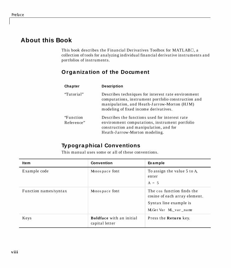
About this BookThis book describes the Financial Derivatives Toolbox for MATLAB, acollection of tools for analyzing individual financial derivative instruments andportfolios of instruments.
Organization of the Document
Typographical ConventionsThis manual uses some or all of these conventions.
Chapter Description
“Tutorial” Describes techniques for interest rate environmentcomputations, instrument portfolio construction andmanipulation, and Heath-Jarrow-Morton (HJM)modeling of fixed income derivatives.
“FunctionReference”
Describes the functions used for interest rateenvironment computations, instrument portfolioconstruction and manipulation, and forHeath-Jarrow-Morton modeling.
Item Convention Example
Example code Monospace font To assign the value 5 to A,enter
A = 5
Function names/syntax Monospace font The cos function finds thecosine of each array element.
Syntax line example is
MLGetVar ML_var_name
Keys Boldface with an initialcapital letter
Press the Return key.

About this Book
ix
Literal strings (in syntaxdescriptions in referencechapters)
Monospace bold forliterals
f = freqspace(n,'whole')
Mathematicalexpressions
Italics for variables
Standard text font forfunctions, operators, andconstants
This vector represents thepolynomial
p = x2 + 2x + 3
MATLAB output Monospace font MATLAB responds with
A =
5
Menu names, menu items, andcontrols
Boldface with an initialcapital letter
Choose the File menu.
New terms Italics An array is an orderedcollection of information.
String variables (from a finitelist)
Monospace italics sysc = d2c(sysd, 'method')
Item Convention Example

Preface
x
Related ProductsThe MathWorks provides several products relevant to the tasks you canperform with the Financial Derivatives Toolbox.
For more information about any of these products, see either:
• The online documentation for that product, if it is installed or if you arereading the documentation from the CD
• The MathWorks Web site, at http://www.mathworks.com; see the “products”section
Note The toolboxes listed below all include functions that extend MATLAB’scapabilities.
Product Description
Database Toolbox Tool for connecting to, and interacting with,most ODBC/JDBC databases from withinMATLAB
Datafeed Toolbox MATLAB functions for integrating thenumerical, computational, and graphicalcapabilities of MATLAB with financial dataproviders
Excel Link Tool that integrates MATLAB capabilities withMicrosoft Excel for Windows
Financial Time SeriesToolbox
Tool for analyzing time series data in thefinancial markets
Financial Toolbox MATLAB functions for quantitative financialmodeling and analytic prototyping

Related Products
xi
GARCH Toolbox MATLAB functions for univariate GeneralizedAutoregressive Conditional Heteroskedasticity(GARCH) volatility modeling
MATLAB Integrated technical computing environmentthat combines numeric computation, advancedgraphics and visualization, and a high-levelprogramming language
MATLAB Compiler Compiler for automatically convertingMATLAB M-files to C and C++ code
MATLAB ReportGenerator
Tool for documenting information in MATLABin multiple output formats
MATLAB RuntimeServer
MATLAB environment in which you can takean existing MATLAB application and turn itinto a stand-alone product that is easy andcost-effective to package and distribute. Usersaccess only the features that you provide viayour application’s graphical user interface(GUI). They do not have access to your code orthe MATLAB command line.
Optimization Toolbox Tool for general and large-scale optimization ofnonlinear problems, as well as for linearprogramming, quadratic programming,nonlinear least squares, and solving nonlinearequations
Spline Toolbox Tool for the construction and use of piecewisepolynomial functions
Statistics Toolbox Tool for analyzing historical data, modelingsystems, developing statistical algorithms, andlearning and teaching statistics
Product Description

Preface
xii
Further Reading
Heath-Jarrow-Morton ModelingAn introduction to Heath-Jarrow-Morton (HJM) modeling, used extensively inthe Financial Derivatives Toolbox, can be found in:
Jarrow, Robert A., Modelling Fixed Income Securities and Interest RateOptions, McGraw-Hill, 1996, ISBN 0-07-912253-1.
Financial DerivativesInformation on the creation of financial derivatives and their role in themarketplace can be found in numerous sources. Among those consulted in thedevelopment of the Financial Derivatives toolbox are:
Chance, Don. M., An Introduction to Derivatives, The Dryden Press, 1998,ISBN 0-030-024483-8
Fabozzi, Frank J., Treasury Securities and Derivatives, Frank J. FabozziAssociates, 1998, ISBN 1-883249-23-6
Hull, John C., Options, Futures, and Other Derivatives, Prentice-Hall, 1997,ISBN 0-13-186479-3
Wilmott, Paul, Derivatives: The Theory and Practice of Financial Engineering,John Wiley and Sons, 1998, ISBN 0-471-983-89-6
1
Tutorial
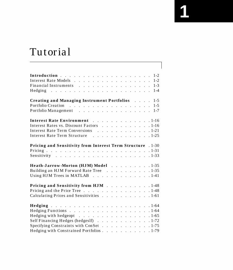
Introduction . . . . . . . . . . . . . . . . . . . . 1-2Interest Rate Models . . . . . . . . . . . . . . . . . 1-2Financial Instruments . . . . . . . . . . . . . . . . 1-3Hedging . . . . . . . . . . . . . . . . . . . . . . 1-4
Creating and Managing Instrument Portfolios . . . . 1-5Portfolio Creation . . . . . . . . . . . . . . . . . . 1-5Portfolio Management . . . . . . . . . . . . . . . . 1-7
Interest Rate Environment . . . . . . . . . . . . . 1-16Interest Rates vs. Discount Factors . . . . . . . . . . . 1-16Interest Rate Term Conversions . . . . . . . . . . . . 1-21Interest Rate Term Structure . . . . . . . . . . . . . 1-25
Pricing and Sensitivity from Interest Term Structure . 1-30Pricing . . . . . . . . . . . . . . . . . . . . . . . 1-31Sensitivity . . . . . . . . . . . . . . . . . . . . . 1-33
Heath-Jarrow-Morton (HJM) Model . . . . . . . . . 1-35Building an HJM Forward Rate Tree . . . . . . . . . . 1-35Using HJM Trees in MATLAB . . . . . . . . . . . . . 1-41
Pricing and Sensitivity from HJM . . . . . . . . . . 1-48Pricing and the Price Tree . . . . . . . . . . . . . . . 1-48Calculating Prices and Sensitivities . . . . . . . . . . . 1-61
Hedging . . . . . . . . . . . . . . . . . . . . . . 1-64Hedging Functions . . . . . . . . . . . . . . . . . . 1-64Hedging with hedgeopt . . . . . . . . . . . . . . . . 1-65Self Financing Hedges (hedgeslf) . . . . . . . . . . . . 1-72Specifying Constraints with ConSet . . . . . . . . . . . 1-75Hedging with Constrained Portfolios . . . . . . . . . . . 1-79

1 Tutorial
1-2
IntroductionThe Financial Derivatives Toolbox extends the Financial Toolbox in the areasof fixed income derivatives and of securities contingent upon interest rates.The toolbox provides components for analyzing individual financial derivativeinstruments and portfolios. Specifically, it provides the necessary functions forcalculating prices and sensitivities, for hedging, and for visualizing results.
Interest Rate ModelsThe Financial Derivatives Toolbox computes pricing and sensitivities ofinterest rate contingent claims based upon sets of zero coupon bonds or theHeath-Jarrow-Morton (HJM) evolution model of the interest rate termstructure. For information, see:
• “Pricing and Sensitivity from Interest Term Structure” on page 1-30 for adiscussion of price and sensitivity based upon portfolios of zero couponbonds.
• “Pricing and Sensitivity from HJM” on page 1-48 for a discussion of price andsensitivity based upon the HJM model.
TreesThe Heath-Jarrow-Morton model works with a type of interest rate tree calleda bushy tree. A bushy tree is a tree in which the number of branches increasesexponentially relative to observation times; branches never recombine. Theopposite of a bushy tree is a recombining tree, a tree in which branchesrecombine over time. From any given node, the node reached by taking thepath up-down is the same node reached by taking the path down-up. A bushyand a recombining tree are both illustrated in the next figure.

Introduction
1-3
Financial InstrumentsThe toolbox provides a set of functions that perform computations uponportfolios containing up to seven types of financial instruments.
Bond. A long-term debt security with preset interest rate and maturity, bywhich the principal and interest must be paid.
Bond Options. Puts and calls on portfolios of bonds.
Fixed Rate Note. A long-term debt security with preset interest rate andmaturity, by which the interest must be paid. The principal may or may not bepaid at maturity. In this version of the Financial Derivatives Toolbox, theprincipal is always paid at maturity.
Floating Rate Note. A security similar to a bond, but in which the note’s interestrate is reset periodically, relative to a reference index rate, to reflectfluctuations in market interest rates.
Cap. A contract which includes a guarantee that sets the maximum interestrate to be paid by the holder, based upon an otherwise floating interest rate.
Floor. A contract which includes a guarantee setting the minimum interest rateto be received by the holder, based upon an otherwise floating interest rate.
Bushy Tree
Recombining Tree

1 Tutorial
1-4
Swap. A contract between two parties obligating the parties to exchange futurecash flows. This version of the Financial Derivatives Toolbox handles only thevanilla swap, which is composed of a floating rate leg and a fixed rate leg.
Additionally, the toolbox provides functions for the creation and pricing ofarbitrary cash flow instruments based upon zero coupon bonds or upon theHJM model.
HedgingThe Financial Derivatives Toolbox also includes hedging functionality,allowing the rebalancing of portfolios to reach target costs or targetsensitivities, which may be set to zero for a neutral-sensitivity portfolio.Optionally, the rebalancing process can be self-financing or directed by a set ofuser-supplied constraints. For information, see:
• “Hedging” on page 1-64 for a discussion of the hedging process.
• “hedgeopt” on page 2-42 for a description of the function that allocates anoptimal hedge.
• “hedgeslf” on page 2-45 for a description of the function that allocates aself-financing hedge.

Creating and Managing Instrument Portfolios
1-5
Creating and Managing Instrument PortfoliosThe Financial Derivatives Toolbox provides components for analyzingindividual derivative instruments and portfolios containing several types offinancial instruments. The toolbox provides functionality that supports thecreation and management of these instruments:
• Bonds
• Bond Options
• Fixed Rate Notes
• Floating Rate Notes
• Caps
• Floors
• Swaps
Additionally, the toolbox provides functions for the creation of arbitrary cashflow instruments.
The toolbox also provides pricing and sensitivity routines for theseinstruments. (See “Pricing and Sensitivity from Interest Term Structure” onpage 1-30 and “Pricing and Sensitivity from HJM” on page 1-48.)
Portfolio CreationThe instadd function creates a set of instruments (portfolio) or addsinstruments to an existing instrument collection. The TypeString argumentspecifies the type of the investment instrument: 'Bond', 'OptBond','CashFlow', 'Fixed', 'Float', 'Cap', 'Floor', or 'Swap'. The inputarguments following TypeString are specific to the type of investmentinstrument. Thus, the TypeString argument determines how the remainderof the input arguments is interpreted.
For example, instadd with the type string 'Bond' creates a portfolio of bondinstruments
InstSet = instadd('Bond', CouponRate, Settle, Maturity, Period,Basis, EndMonthRule, IssueDate, FirstCouponDate, LastCouponDate,StartDate, Face)

1 Tutorial
1-6
In a similar manner, instadd can create portfolios of other types of investmentinstruments:
• Bond option
InstSet = instadd('OptBond', BondIndex, OptSpec, Strike,ExerciseDates, AmericanOpt)
• Arbitrary cash flow instrument
InstSet = instadd('CashFlow', CFlowAmounts, CFlowDates, Settle,Basis)
• Fixed rate note instrumentInstSet = instadd('Fixed', CouponRate, Settle, Maturity,FixedReset, Basis, Principal)
• Floating rate note instrumentInstSet = instadd('Float', Spread, Settle, Maturity, FloatReset,Basis, Principal)
• Cap instrumentInstSet = instadd('Cap', Strike, Settle, Maturity, CapReset,Basis, Principal)
• Floor instrumentInstSet = instadd('Floor', Strike, Settle, Maturity, FloorReset,Basis, Principal)
• Swap instrument
InstSet = instadd('Swap', LegRate, Settle, Maturity, LegReset,Basis, Principal, LegType)
To use the instadd function to add additional instruments to an existinginstrument portfolio, provide the name of an existing portfolio as the firstargument to the instadd function.
Consider, for example, a portfolio containing two cap instruments only.

Creating and Managing Instrument Portfolios
1-7
Strike = [0.06; 0.07];Settle = '08-Feb-2000';Maturity = '15-Jan-2003';
Port_1 = instadd('Cap', Strike, Settle, Maturity);
These commands create a portfolio containing two cap instruments with thesame settlement and maturity dates, but with different strikes. In general, theinput arguments describing an instrument can be either a scalar, or a numberof instruments (NumInst)-by-1 vector in which each element corresponds to aninstrument. Using a scalar assigns the same value to all instruments passed inthe call to instadd.
Use the instdisp command to display the contents of the instrument set.
instdisp(Port_1)
Index Type Strike Settle Maturity CapReset Basis Principal1 Cap 0.06 08-Feb-2000 15-Jan-2003 NaN NaN NaN2 Cap 0.07 08-Feb-2000 15-Jan-2003 NaN NaN NaN
Now add a single bond instrument to Port_1. The bond has a 4.0% coupon andthe same settlement and maturity dates as the cap instruments.
CouponRate = 0.04;Port_1 = instadd(Port_1, 'Bond', CouponRate, Settle, Maturity);
Use instdisp again to see the resulting instrument set.
instdisp(Port_1)
Index Type Strike Settle Maturity CapReset Basis Principal1 Cap 0.06 08-Feb-2000 15-Jan-2003 NaN NaN NaN2 Cap 0.07 08-Feb-2000 15-Jan-2003 NaN NaN NaN
Index Type CouponRate Settle Maturity Period Basis ...3 Bond 0.04 08-Feb-2000 15-Jan-2003 NaN NaN ...
Portfolio ManagementThe portfolio management capabilities provided by the Financial Derivativestoolbox include:

1 Tutorial
1-8
• Constructors for the most common financial instruments. (See “InstrumentConstructors” on page 1-8.)
• The ability to create new instruments or to add new fields to existinginstruments. (See “Creating New Instruments or Properties” on page 1-9.)
• The ability to search or subset a portfolio. See “Searching or Subsetting aPortfolio” on page 1-11.)
Instrument ConstructorsThe toolbox provides constructors for the most common financial instruments.
Note A constructor is a function that builds a structure dedicated to a certaintype of object; in this toolbox, an object is a type of market instrument.
The instruments and their constructors in this toolbox are listed below.
Each instrument has parameters (fields) that describe the instrument. Thetoolbox functions enable you to:
• Create an instrument or portfolio of instruments
• Enumerate stored instrument types and information fields
• Enumerate instrument field data
• Search and select instruments
Instrument Constructor
Bond instbond
Bond option instoptbnd
Arbitrary cash flow instcf
Fixed rate note instfixed
Floating rate note instfloat
Cap instcap
Floor instfloor
Swap instswap

Creating and Managing Instrument Portfolios
1-9
The instrument structure consists of various fields according to instrumenttype. A field is an element of data associated with the instrument. For example,a bond instrument contains the fields CouponRate, Settle, Maturity, etc.Additionally, each instrument has a field that identifies the investment type(bond, cap, floor, etc.).
In reality the set of parameters for each instrument is not fixed. Users have theability to add additional parameters. These additional fields will be ignored bythe toolbox functions. They may be used to attach additional information toeach instrument, such as an internal code describing the bond.
Parameters not specified when creating an instrument default to NaN, which,in general, means that the functions using the instrument set (such asintenvprice or hjmprice) will use default values. At the time of pricing, anerror occurs if any of the required fields is missing, such as Strike in a cap, orthe CouponRate in a bond.
Creating New Instruments or PropertiesUse the instaddfield function to create a new kind of instrument or to addnew parameters to the instruments in an existing instrument collection.
To create a new kind of instrument with instaddfield, you need to specifythree arguments: 'Type', 'FieldName', and 'Data'. 'Type' defines the type ofthe new instrument, for example, Future. 'FieldName' names the fieldsuniquely associated with the new type of instrument. 'Data' contains the datafor the fields of the new instrument.
An optional fourth parameter is 'ClassList'. 'ClassList' specifies the datatypes of the contents of each unique field for the new instrument.
Here are the syntaxes to create a new kind of instrument using instaddfield.
InstSet = instaddfield('FieldName', FieldList, 'Data', DataList,'Type', TypeString)
InstSet = instaddfield('FieldName', FieldList, 'FieldClass',ClassList, 'Data' , DataList, 'Type', TypeString)
And, to add new instruments to an existing set, use
InstSetNew = instaddfield(InstSetOld, 'FieldName', FieldList,'Data', DataList, 'Type', TypeString)

1 Tutorial
1-10
As an example, consider a futures contract with a delivery date of July 15,2000, and a quoted price of $104.40. Since the Financial Derivatives Toolboxdoes not directly support this instrument, you must create it using the functioninstaddfield. The parameters used for the creation of the instruments are:
• Type: Future
• Field names: Delivery and Price
• Data: Delivery is July 15, 2000, and Price is $104.40.
Enter the data into MATLAB.
Type = 'Future';FieldName = {'Delivery', 'Price'};Data = {'Jul-15-2000', 104.4};
Optionally, you can also specify the data types of the data cell array by creatinganother cell array containing this information.
FieldClass = {'date','dble'};
Finally, create the portfolio with a single instrument.
Port = instaddfield('Type', Type, 'FieldName', FieldName,...'FieldClass', FieldClass, 'Data', Data);
Now use the function instdisp to examine the resulting single-instrumentportfolio.
instdisp(Port)
Index Type Delivery Price1 Future 15-Jul-2000 104.4
Because your portfolio Port has the same structure as those created using thefunction instadd, you can combine portfolios created using instadd withportfolios created using instaddfield. For example, you can now add two capinstruments to Port with instadd.
Strike = [0.06; 0.07];Settle = '08-Feb-2000';Maturity = '15-Jan-2003';
Port = instadd(Port, 'Cap', Strike, Settle, Maturity);

Creating and Managing Instrument Portfolios
1-11
View the resulting portfolio using instdisp.
instdisp(Port)
Index Type Delivery Price1 Future 15-Jul-2000 104.4
Index Type Strike Settle Maturity CapReset Basis Pricipal2 Cap 0.06 08-Feb-2000 15-Jan-2003 NaN NaN NaN3 Cap 0.07 08-Feb-2000 15-Jan-2003 NaN NaN NaN
Searching or Subsetting a PortfolioThe Financial Derivatives Toolbox provides functions that enable you to:
• Find specific instruments within a portfolio
• Create a subset portfolio consisting of instruments selected from a largerportfolio
The instfind function finds instruments with a specific parameter value; itreturns an instrument index (position) in a large instrument set. Theinstselect function, on the other hand, subsets a large instrument set into aportfolio of instruments with designated parameter values; it returns aninstrument set (portfolio) rather than an index.
instfind. The general syntax for instfind is
IndexMatch = instfind(InstSet, 'FieldName', FieldList, 'Data',DataList, 'Index', IndexSet, 'Type', TypeList)
InstSet is the instrument set to search. Within InstSet instruments arecategorized by type, and each type can have different data fields. The storeddata field is a row vector or string for each instrument.
The FieldList, DataList, and TypeList arguments indicate values to searchfor in the 'FieldName', 'Data', and 'Type' data fields of the instrument set.FieldList is a cell array of field name(s) specific to the instruments. DataListis a cell array or matrix of acceptable values for the parameter(s) specified inFieldList. 'FieldName' and 'Data' (consequently, FieldList and DataList)parameters must appear together or not at all.
IndexSet is a vector of integer index(es) designating positions of instrumentsin the instrument set to check for matches; the default is all indices available

1 Tutorial
1-12
in the instrument set. 'TypeList' is a string or cell array of strings restrictinginstruments to match one of the 'TypeList' types; the default is all types inthe instrument set.
IndexMatch is a vector of positions of instruments matching the input criteria.Instruments are returned in IndexMatch if all the 'FieldName', 'Data','Index', and 'Type' conditions are met. An instrument meets an individualfield condition if the stored 'FieldName' data matches any of the rows listed inthe DataList for that FieldName.
instfind Examples. The example uses the provided MAT-file deriv.mat.
The MAT-file contains an instrument set, HJMInstSet, that contains eightinstruments of seven types.
load deriv.matinstdisp(HJMInstSet)
Find all instruments with a maturity date of January 01, 2003.
Mat2003 = ...instfind(HJMInstSet,'FieldName','Maturity','Data','01-Jan-2003')
Index Type CouponRate Settle Maturity Period Basis ......... Name Quantity1 Bond 0.04 01-Jan-2000 01-Jan-2003 1 NaN......... 4% bond 1002 Bond 0.04 01-Jan-2000 01-Jan-2004 2 NaN......... 4% bond 50
Index Type UnderInd OptSpec Strike ExerciseDates AmericanOpt Name Quantity3 OptBond 2 call 101 01-Jan-2003 NaN Option 101 -50
Index Type CouponRate Settle Maturity FixedReset Basis Principal Name Quantity4 Fixed 0.04 01-Jan-2000 01-Jan-2003 1 NaN NaN 4% Fixed 80
Index Type Spread Settle Maturity FloatReset Basis Principal Name Quantity5 Float 20 01-Jan-2000 01-Jan-2003 1 NaN NaN 20BP Float 8
Index Type Strike Settle Maturity CapReset Basis Principal Name Quantity6 Cap 0.03 01-Jan-2000 01-Jan-2004 1 NaN NaN 3% Cap 30
Index Type Strike Settle Maturity FloorReset Basis Principal Name Quantity7 Floor 0.01 01-Jan-2000 01-Jan-2004 1 NaN NaN 1% Floor 40
Index Type LegRate Settle Maturity LegReset Basis Principal LegType Name Quantity8 Swap [0.04 20] 01-Jan-2000 01-Jan-2003 [1 1] NaN NaN [NaN] 4%/20BP Swap 10

Creating and Managing Instrument Portfolios
1-13
Mat2003 =
1 4 5 8
Find all cap and floor instruments with a maturity date of January 01, 2004.
CapFloor = instfind(HJMInstSet,...'FieldName','Maturity','Data','01-Jan-2004', 'Type',...{'Cap';'Floor'})
CapFloor =
6 7
Find all instruments where the portfolio is long or short a quantity of 50.
Pos50 = instfind(HJMInstSet,'FieldName',...'Quantity','Data',{'50';'-50'})
Pos50 =
2 3
instselect. The syntax for instselect is exactly the same syntax as forinstfind. instselect returns a full portfolio instead of indexes into theoriginal portfolio. Compare the values returned by both functions by callingthem equivalently.
Previously you used instfind to find all instruments in HJMInstSet with amaturity date of January 01, 2003.

1 Tutorial
1-14
Mat2003 = ...instfind(HJMInstSet,'FieldName','Maturity','Data','01-Jan-2003')
Mat2003 =
1 4 5 8
Now use the same instrument set as a starting point, but execute theinstselect function instead, to produce a new instrument set matching theidentical search criteria.
Select2003 = ...instselect(HJMInstSet,'FieldName','Maturity','Data',...'01-Jan-2003')
instdisp(Select2003)
Index Type CouponRate Settle Maturity Period Basis ......... Name Quantity1 Bond 0.04 01-Jan-2000 01-Jan-2003 1 NaN......... 4% bond 100
Index Type CouponRate Settle Maturity FixedReset Basis Principal Name Quantity2 Fixed 0.04 01-Jan-2000 01-Jan-2003 1 NaN NaN 4% Fixed 80
Index Type Spread Settle Maturity FloatReset Basis Principal Name Quantity3 Float 20 01-Jan-2000 01-Jan-2003 1 NaN NaN 20BP Float 8
Index Type LegRate Settle Maturity LegReset Basis Principal LegType Name Quantity4 Swap [0.04 20] 01-Jan-2000 01-Jan-2003 [1 1] NaN NaN [NaN] 4%/20BP Swap 10

Creating and Managing Instrument Portfolios
1-15
instselect Examples. These examples use the portfolio ExampleInst provided withthe MAT-file InstSetExamples.mat.
load InstSetExamples.matinstdisp(ExampleInst)
Index Type Strike Price Opt Contracts1 Option 95 12.2 Call 02 Option 100 9.2 Call 03 Option 105 6.8 Call 1000
Index Type Delivery F Contracts4 Futures 01-Jul-1999 104.4 -1000
Index Type Strike Price Opt Contracts5 Option 105 7.4 Put -10006 Option 95 2.9 Put 0
Index Type Price Maturity Contracts7 TBill 99 01-Jul-1999 6
The instrument set contains three instrument types: 'Option', 'Futures',and 'TBill'. Use instselect to make a new instrument set containing onlyoptions struck at 95. In other words, select all instruments containing the fieldStrike and with the data value for that field equal to 95.
InstSet = instselect(ExampleInst,'FieldName','Strike','Data',95)
instdisp(InstSet)
Index Type Strike Price Opt Contracts1 Option 95 12.2 Call 02 Option 95 2.9 Put 0
You can use all the various forms of instselect and instfind to locate specificinstruments within this instrument set.

1 Tutorial
1-16
Interest Rate EnvironmentThe interest rate environment is the representation of the evolution of interestrates through time. In MATLAB, the interest rate environment isencapsulated in a structure called RateSpec (rate specification). This structureholds all information needed to identify completely the evolution of interestrates. Several functions included in the Financial Derivatives Toolbox arededicated to the creation and management of the RateSpec structure. Manyothers take this structure as an input argument representing the evolution ofinterest rates.
Before looking further at the RateSpec structure, examine three functions thatprovide key functionality for working with interest rates: disc2rate, itsopposite, rate2disc, and ratetimes. The first two functions map betweendiscount rates and interest rates. The third function, ratetimes, calculates theeffect of term changes on the interest rates.
Interest Rates vs. Discount FactorsDiscount factors are coefficients commonly used to find the present value offuture cash flows. As such, there is a direct mapping between the rateapplicable to a period of time, and the corresponding discount factor. Thefunction disc2rate converts discount rates for a given term (period) intointerest rates. The function rate2disc does the opposite; it converts interestrates applicable to a given term (period) into the corresponding discount rates.
Calculating Discount Factors from RatesAs an example, consider these annualized zero coupon bond rates.
From To Rate
15 Feb 2000 15 Aug 2000 0.05
15 Feb 2000 15 Feb 2001 0.056
15 Feb 2000 15 Aug 2001 0.06
15 Feb 2000 15 Feb 2002 0.065
15 Feb 2000 15 Aug 2002 0.075

Interest Rate Environment
1-17
To calculate the discount factors corresponding to these interest rates, callrate2disc using the syntax
Disc = rate2disc(Compounding, Rates, EndDates, StartDates,ValuationDate)
where:
• Compounding represents the frequency at which the zero rates arecompounded when annualized. For this example, assume this value to be 2.
• Rates is a vector of annualized percentage rates representing the interestrate applicable to each time interval.
• EndDates is a vector of dates representing the end of each interest rate term(period).
• StartDates is a vector of dates representing the beginning of each interestrate term.
• ValuationDate is the date of observation for which the discount factors willbe calculated. In this particular example, use February 15, 2000 as thebeginning date for all interest rate terms.
Set the variables in MATLAB.
StartDates = ['15-Feb-2000'];EndDates = ['15-Aug-2000'; '15-Feb-2001'; '15-Aug-2001';...'15-Feb-2002'; '15-Aug-2002'];Compounding = 2;ValuationDate = ['15-Feb-2000'];Rates = [0.05; 0.056; 0.06; 0.065; 0.075];Disc = rate2disc(Compounding, Rates, EndDates, StartDates,...ValuationDate)
Disc =
0.9756 0.9463 0.9151 0.8799 0.8319
1 Tutorial
1-18
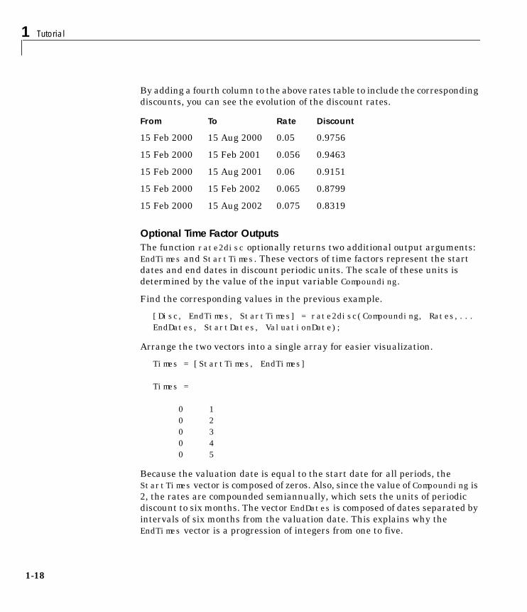
By adding a fourth column to the above rates table to include the correspondingdiscounts, you can see the evolution of the discount rates.
Optional Time Factor OutputsThe function rate2disc optionally returns two additional output arguments:EndTimes and StartTimes. These vectors of time factors represent the startdates and end dates in discount periodic units. The scale of these units isdetermined by the value of the input variable Compounding.
Find the corresponding values in the previous example.
[Disc, EndTimes, StartTimes] = rate2disc(Compounding, Rates,...EndDates, StartDates, ValuationDate);
Arrange the two vectors into a single array for easier visualization.
Times = [StartTimes, EndTimes]
Times =
0 1 0 2 0 3 0 4
0 5
Because the valuation date is equal to the start date for all periods, theStartTimes vector is composed of zeros. Also, since the value of Compounding is2, the rates are compounded semiannually, which sets the units of periodicdiscount to six months. The vector EndDates is composed of dates separated byintervals of six months from the valuation date. This explains why theEndTimes vector is a progression of integers from one to five.
From To Rate Discount
15 Feb 2000 15 Aug 2000 0.05 0.9756
15 Feb 2000 15 Feb 2001 0.056 0.9463
15 Feb 2000 15 Aug 2001 0.06 0.9151
15 Feb 2000 15 Feb 2002 0.065 0.8799
15 Feb 2000 15 Aug 2002 0.075 0.8319

Interest Rate Environment
1-19
Alternative Syntax (rate2disc)The function rate2disc also accommodates an alternative syntax that usesperiodic discount units instead of dates. Since the relationship betweendiscount factors and interest rates is based on time periods and not on absolutedates, this form of rate2disc allows you to work directly with time periods. Inthis mode, the valuation date corresponds to zero, and the vectors StartTimesand EndTimes are used as input arguments instead of their date equivalents,StartDates and EndDates. This syntax for rate2disc is
Disc = rate2disc(Compounding, Rates, EndTimes, StartTimes)
Using as input the StartTimes and EndTimes vectors computed previously, youshould obtain the previous results for the discount factors.
Disc = rate2disc(Compounding, Rates, EndTimes, StartTimes)
Disc =
0.9756 0.9463 0.9151 0.8799 0.8319
Calculating Rates from DiscountsThe function disc2rate is the complement to rate2disc. It finds the ratesapplicable to a set of compounding periods, given the discount factor in thoseperiods. The syntax for calling this function is
Rates = disc2rate(Compounding, Disc, EndDates, StartDates,ValuationDate)
Each argument to this function has the same meaning as in rate2disc. Use theresults found in the previous example to return the rate values you startedwith.
Rates = disc2rate(Compounding, Disc, EndDates, StartDates,...ValuationDate)

1 Tutorial
1-20
Rates =
0.0500 0.0560 0.0600 0.0650 0.0750
Alternative Syntax (disc2rate)As in the case of rate2disc, disc2rate optionally returns StartTimes andEndTimes vectors representing the start and end times measured in discountperiodic units. Again, working with the same values as before, you shouldobtain the same numbers.
[Rates, EndTimes, StartTimes] = disc2rate(Compounding, Disc,...EndDates, StartDates, ValuationDate);
Arrange the results in a matrix convenient to display.
Result = [StartTimes, EndTimes, Rates]
Result =
0 1.0000 0.0500 0 2.0000 0.0560 0 3.0000 0.0600 0 4.0000 0.0650 0 5.0000 0.0750
As with rate2disc, the relationship between rates and discount factors isdetermined by time periods and not by absolute dates. Consequently, thealternate syntax for disc2rate uses time vectors instead of dates, and itassumes that the valuation date corresponds to time = 0. The times-basedcalling syntax is:
Rates = disc2rate(Compounding, Disc, EndTimes, StartTimes);
Using this syntax, we again obtain the original values for the interest rates.

Interest Rate Environment
1-21
Rates = disc2rate(Compounding, Disc, EndTimes, StartTimes)
Rates =
0.0500 0.0560 0.0600 0.0650 0.0750
Interest Rate Term ConversionsInterest rate evolution is typically represented by a set of interest rates,including the beginning and end of the periods the rates apply to. For zerorates, the start dates are typically at the valuation date, with the ratesextending from that valuation date until their respective maturity dates.
Calculating Rates Applicable to Different PeriodsFrequently, given a set of rates including their start and end dates, you may beinterested in finding the rates applicable to different terms (periods). Thisproblem is addressed by the function ratetimes. This function interpolates theinterest rates given a change in the original terms. The syntax for callingratetimes is
[Rates, EndTimes, StartTimes] = ratetimes(Compounding, RefRates,RefEndDates, RefStartDates, EndDates, StartDates,ValuationDate);
where:
• Compounding represents the frequency at which the zero rates arecompounded when annualized.
• RefRates is a vector of initial interest rates representing the interest ratesapplicable to the initial time intervals.
• RefEndDates is a vector of dates representing the end of the interest rateterms (period) applicable to RefRates.
• RefStartDates is a vector of dates representing the beginning of the interestrate terms applicable to RefRates.

1 Tutorial
1-22
• EndDates represent the maturity dates for which the interest rates will beinterpolated.
• StartDates represent the starting dates for which the interest rates will beinterpolated.
• ValuationDate is the date of observation, from which the StartTimes andEndTimes will be calculated. This date represents time = 0.
The input arguments to this function can be separated into two groups:
1 The initial or reference interest rates, including the terms for which they arevalid
2 Terms for which the new interest rates will be calculated
As an example, consider the rate table specified earlier.
Assuming that the valuation date is February 15, 2000, these rates representzero coupon bond rates with maturities specified in the second column. Use thefunction ratetimes to calculate the spot rates at the beginning of all periodsimplied in the table. Assume a compounding value of 2.
% Reference Rates.RefStartDates = ['15-Feb-2000'];RefEndDates = ['15-Aug-2000'; '15-Feb-2001'; '15-Aug-2001';...'15-Feb-2002'; '15-Aug-2002'];Compounding = 2;ValuationDate = ['15-Feb-2000'];RefRates = [0.05; 0.056; 0.06; 0.065; 0.075];
From To Rate
15 Feb 2000 15 Aug 2000 0.05
15 Feb 2000 15 Feb 2001 0.056
15 Feb 2000 15 Aug 2001 0.06
15 Feb 2000 15 Feb 2002 0.065
15 Feb 2000 15 Aug 2002 0.075

Interest Rate Environment
1-23
% New Terms.StartDates = ['15-Feb-2000'; '15-Aug-2000'; '15-Feb-2001';...'15-Aug-2001'; '15-Feb-2002'];EndDates = ['15-Aug-2000'; '15-Feb-2001'; '15-Aug-2001';...'15-Feb-2002'; '15-Aug-2002'];
% Find the new rates.[Rates, EndTimes, StartTimes] = ratetimes(Compounding, ...RefRates, RefEndDates, RefStartDates, EndDates, StartDates,...ValuationDate);
Rates =
0.0500 0.0620 0.0680 0.0801 0.1155
Place these values in a table similar to the one above. Observe the evolution ofthe spot rates based on the initial zero coupon rates.
Alternative Syntax (ratetimes)The additional output arguments StartTimes and EndTimes represent the timefactor equivalents to the StartDates and EndDates vectors. As with thefunctions disc2rate and rate2disc, ratetimes uses time factors forinterpolating the rates. These time factors are calculated from the start andend dates, and the valuation date, which are passed as input arguments.ratetimes also has an alternate syntax that uses time factors directly, andassumes time = 0 as the valuation date. This alternate syntax is
From To Rate
15 Feb 2000 15 Aug 2000 0.0500
15 Aug 2000 15 Feb 2001 0.0620
15 Feb 2001 15 Aug 2001 0.0680
15 Aug 2001 15 Feb 2002 0.0801
15 Feb 2002 15 Aug 2002 0.1155

1 Tutorial
1-24
[Rates, EndTimes, StartTimes] = ratetimes(Compounding, RefRates,RefEndTimes, RefStartTimes, EndTimes, StartTimes);
Use this alternate version of ratetimes to find the spot rates again. In thiscase, you must first find the time factors of the reference curve. Use date2timefor this.
RefEndTimes = date2time(ValuationDate, RefEndDates, Compounding)
RefEndTimes =
1 2 3 4 5
RefStartTimes = date2time(ValuationDate, RefStartDates,...Compounding)
RefStartTimes =
0
These are the expected values, given semiannual discounts (as denoted by avalue of 2 in the variable Compounding), end dates separated by six-monthperiods, and the valuation date equal to the date marking beginning of the firstperiod (time factor = 0).
Now call ratetimes with the alternate syntax.
[Rates, EndTimes, StartTimes] = ratetimes(Compounding,...RefRates, RefEndTimes, RefStartTimes, EndTimes, StartTimes);
Rates =
0.0500 0.0620 0.0680 0.0801 0.1155

Interest Rate Environment
1-25
EndTimes and StartTimes have, as expected, the same values they had as inputarguments.
Times = [StartTimes, EndTimes]
Times =
0 1 1 2 2 3 3 4
4 5
Interest Rate Term StructureThe Financial Derivatives Toolbox includes a set of functions to encapsulateinterest rate term information into a single structure. These functions presenta convenient way to package all information related to interest rate terms intoa common format, and to resolve interdependencies when one or more of theparameters is modified. For information, see:
• “Creation or Modification (intenvset)” on page 1-25 for a discussion of how tocreate or modify an interest rate term structure (RateSpec) using theintenvset function.
• “Obtaining Specific Properties (intenvget)” on page 1-27 for a discussion ofhow to extract specific properties from a RateSpec.
Creation or Modification (intenvset)The main function to create or modify an interest rate term structure RateSpec(rates specification) is intenvset. If the first argument to this function is apreviously created RateSpec, the function modifies the existing ratespecification and returns a new one. Otherwise, it creates a new RateSpec. Theother intenvset arguments are property-value pairs, indicating the new valuefor these properties. The properties that can be specified or modified are:
• Compounding• Disc• Rates

1 Tutorial
1-26
• EndDates• StartDates• ValuationDate• Basis• EndMonthRule
To learn about the properties EndMonthRule and Basis, type helpftbEndMonthRule and help ftbBasis or see the Financial Toolbox User'sGuide.
Consider again the original table of interest rates.
Use the information in this table to populate the RateSpec structure.
StartDates = ['15-Feb-2000'];EndDates = ['15-Aug-2000';
'15-Feb-2001';'15-Aug-2001';'15-Feb-2002';'15-Aug-2002'];
Compounding = 2;ValuationDate = ['15-Feb-2000'];Rates = [0.05; 0.056; 0.06; 0.065; 0.075];
rs = intenvset('Compounding',Compounding,'StartDates',...StartDates, 'EndDates', EndDates, 'Rates', Rates,...'ValuationDate', ValuationDate)
From To Rate
15 Feb 2000 15 Aug 2000 0.05
15 Feb 2000 15 Feb 2001 0.056
15 Feb 2000 15 Aug 2001 0.06
15 Feb 2000 15 Feb 2002 0.065
15 Feb 2000 15 Aug 2002 0.075

Interest Rate Environment
1-27
rs =
FinObj:'RateSpec'Compounding:2
Disc:[5x1 double]Rates:[5x1 double]
EndTimes:[5x1 double]StartTimes:[5x1 double]
EndDates:[5x1 double]StartDates:730531
ValuationDate:730531Basis: 0
EndMonthRule: 1
Some of the properties filled in the structure were not passed explicitly in thecall to RateSpec. The values of the automatically completed properties dependupon the properties that are explicitly passed. Consider for example theStartTimes and EndTimes vectors. Since the StartDates and EndDates vectorsare passed in, as well as the ValuationDate, intenvset has all the informationneeded to calculate StartTimes and EndTimes. Hence, these two properties areread-only.
Obtaining Specific Properties (intenvget)The complementary function to intenvset is intenvget. This function obtainsspecific properties from the interest rate term structure. The syntax of thisfunction is
ParameterValue = intenvget(RateSpec, 'ParameterName')
To obtain the vector EndTimes from the RateSpec structure, enter
EndTimes = intenvget(rs, 'EndTimes')
EndTimes =
1 2 3 4 5

1 Tutorial
1-28
To obtain Disc, the values for the discount factors that were calculatedautomatically by intenvset, type
Disc = intenvget(rs, 'Disc')
Disc =
0.9756 0.9463 0.9151 0.8799 0.8319
These discount factors correspond to the periods starting from StartDates andending in EndDates.
Note Although it is possible to access directly these fields within thestructure, instead of using intenvget, we strongly advise against this. Theformat of the interest rate term structure could change in future versions ofthe toolbox. Should that happen, any code accessing the RateSpec fieldsdirectly would stop working.
Now use the RateSpec structure with its functions to examine how changes inspecific properties of the interest rate term structure affect those dependingupon it. As an exercise, change the value of Compounding from 2 (semiannual)to 1 (annual).
rs = intenvset(rs, 'Compounding', 1);
Since StartTimes and EndTimes are measured in units of periodic discount, achange in Compounding from 2 to 1 redefines the basic unit from semiannual toannual. This means that a period of six months is represented with a value of0.5, and a period of one year is represented by 1. To obtain the vectorsStartTimes and EndTimes, enter
StartTimes = intenvget(rs, 'StartTimes');EndTimes = intenvget(rs, 'EndTimes');
Interest Rate Environment
1-29
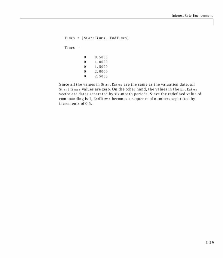
Times = [StartTimes, EndTimes]
Times =
0 0.5000 0 1.0000 0 1.5000 0 2.0000
0 2.5000
Since all the values in StartDates are the same as the valuation date, allStartTimes values are zero. On the other hand, the values in the EndDatesvector are dates separated by six-month periods. Since the redefined value ofcompounding is 1, EndTimes becomes a sequence of numbers separated byincrements of 0.5.

1 Tutorial
1-30
Pricing and Sensitivity from Interest Term StructureThe Financial Derivatives Toolbox contains a family of functions that finds theprice and sensitivities of several financial instruments based on interest ratecurves. For information, see:
• “Pricing” on page 1-31 for a discussion on using the intenvprice function toprice a portfolio of instruments based on a set of zero curves.
• “Sensitivity” on page 1-33 for a discussion on computing delta and gammasensitivities with the intenvsens function.
The instruments can be presented to the functions as a portfolio of differenttypes of instruments or as groups of instruments of the same type. The currentversion of the toolbox can compute price and sensitivities for four instrumenttypes using interest rate curves:
• Bonds
• Fixed Rate Notes
• Floating Rate Notes
• Swaps
In addition to these instruments, the toolbox also supports the calculation ofprice and sensitivities of arbitrary sets of cash flows.
Note that options and interest rates floors and caps are absent from the abovelist of supported instruments. These instruments are not supported becausetheir pricing and sensitivity function require a stochastic model for theevolution of interest rates. The interest rate term structure used for pricing istreated as deterministic, and as such is not adequate for pricing theseinstruments.
The Financial Derivatives Toolbox additionally contains functions that use theHeath-Jarrow-Morton (HJM) model to compute prices and sensitivities forfinancial instruments. The HJM model supports computations involvingoptions and interest rate floors and caps. See “Pricing and Sensitivity fromHJM” on page 1-48 for information on computing price and sensitivities offinancial instruments using the Heath-Jarrow-Morton model.
Pricing and Sensitivity from Interest Term Structure
1-31
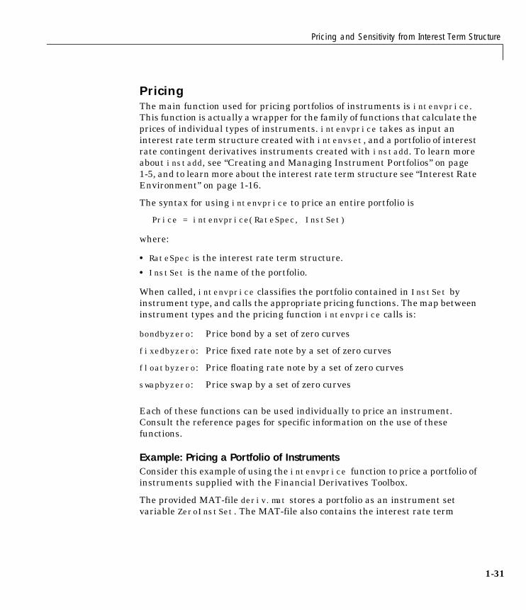
PricingThe main function used for pricing portfolios of instruments is intenvprice.This function is actually a wrapper for the family of functions that calculate theprices of individual types of instruments. intenvprice takes as input aninterest rate term structure created with intenvset, and a portfolio of interestrate contingent derivatives instruments created with instadd. To learn moreabout instadd, see “Creating and Managing Instrument Portfolios” on page1-5, and to learn more about the interest rate term structure see “Interest RateEnvironment” on page 1-16.
The syntax for using intenvprice to price an entire portfolio is
Price = intenvprice(RateSpec, InstSet)
where:
• RateSpec is the interest rate term structure.
• InstSet is the name of the portfolio.
When called, intenvprice classifies the portfolio contained in InstSet byinstrument type, and calls the appropriate pricing functions. The map betweeninstrument types and the pricing function intenvprice calls is:
Each of these functions can be used individually to price an instrument.Consult the reference pages for specific information on the use of thesefunctions.
Example: Pricing a Portfolio of InstrumentsConsider this example of using the intenvprice function to price a portfolio ofinstruments supplied with the Financial Derivatives Toolbox.
The provided MAT-file deriv.mat stores a portfolio as an instrument setvariable ZeroInstSet. The MAT-file also contains the interest rate term
bondbyzero: Price bond by a set of zero curves
fixedbyzero: Price fixed rate note by a set of zero curves
floatbyzero: Price floating rate note by a set of zero curves
swapbyzero: Price swap by a set of zero curves

1 Tutorial
1-32
structure ZeroRateSpec. You can display the instruments with the functioninstdisp.
load deriv.mat;instdisp(ZeroInstSet)
Index Type CouponRate Settle Maturity Period Basis...1 Bond 0.04 01-Jan-2000 01-Jan-2003 1 NaN...2 Bond 0.04 01-Jan-2000 01-Jan-2004 2 NaN...
Index Type CouponRate Settle Maturity FixedReset Basis...3 Fixed 0.04 01-Jan-2000 01-Jan-2003 1 NaN...
Index Type Spread Settle Maturity FloatReset Basis...4 Float 20 01-Jan-2000 01-Jan-2003 1 NaN...
Index Type LegRate Settle Maturity LegReset Basis...5 Swap [0.04 20] 01-Jan-2000 01-Jan-2003 [1 1] NaN...
Use intenvprice to calculate the prices for the instruments contained in theportfolio ZeroInstSet.
format bankPrices = intenvprice(ZeroRateSpec, ZeroInstSet)Prices =
105.77 107.69 105.77 100.58 5.19
The output Prices is a vector containing the prices of all the instruments inthe portfolio in the order indicated by the Index column displayed by instdisp.Consequently, the first two elements in Prices correspond to the first twobonds; the third element corresponds to the fixed rate note; the fourth to thefloating rate note; and the fifth element corresponds to the price of the swap.

Pricing and Sensitivity from Interest Term Structure
1-33
SensitivityThe Financial Derivatives Toolbox can calculate two types of derivative pricesensitivities, namely delta and gamma. Delta represents the dollar sensitivityof prices to shifts in the observed forward yield curve. Gamma represents thedollar sensitivity of delta to shifts in the observed forward yield curve.
The intenvsens function computes instrument sensitivities as well asinstrument prices. If you need both the prices and sensitivity measures, useintenvsens. A separate call to intenvprice is not required.
Here is the syntax
[Delta, Gamma, Price] = intenvsens(RateSpec, InstSet)
where, as before:
• RateSpec is the interest rate term structure
• InstSet is the name of the portfolio
Example: Sensitivities and PricesHere is an example of using intenvsens to calculate both sensitivities andprices.
format longload deriv.mat;[Delta, Gamma, Price] = intenvsens(ZeroRateSpec, ZeroInstSet);
Display the results in a single matrix in long format.
All = [Delta Gamma Price]
All =
1.0e+003 *
-0.29971721334060 1.16033886010257 0.10576776654530-0.39585159618412 1.90136650339994 0.10769123495924-0.29971721334060 1.16033886010257 0.10576776654530-0.00112373852341 0.00366003366949 0.10057677665453-0.29859347481719 1.15667882643308 0.00519098989077

1 Tutorial
1-34
To view the per-dollar sensitivity, divide the first two columns by the last one.
[Delta./Price, Gamma./Price, Price]
ans =
1.0e+002 *
-0.02833729245973 0.10970628368196 1.05767766545296 -0.03675801436709 0.17655721973284 1.07691234959241 -0.02833729245973 0.10970628368196 1.05767766545296 -0.00011172942311 0.00036390445103 1.00576776654530 -0.57521490332382 2.22824326529828 0.05190989890766

Heath-Jarrow-Morton (HJM) Model
1-35
Heath-Jarrow-Morton (HJM) ModelThe Heath-Jarrow-Morton (HJM) model is one of the most widely used modelsfor pricing interest rate derivatives. The model considers a given initial termstructure of interest rates and a specification of the volatility of forward ratesto build a tree representing the evolution of the interest rates, based upon astatistical process. For further explanation, see the book “Modelling FixedIncome Securities and Interest Rate Options” by Robert A. Jarrow.
Building an HJM Forward Rate TreeThe HJM tree of forward rates is the fundamental unit representing theevolution of interest rates in a given period of time. This section explains howto create the HJM forward rate tree using the Financial Derivatives Toolbox.
The MATLAB function that creates the HJM forward rate tree is hjmtree. Thisfunction takes three structures as input arguments:
1 The volatility model VolSpec. (See “Specifying the Volatility Model(VolSpec)” on page 1-36.)
2 The interest rate term structure RateSpec. (See “Specifying the InterestRate Term Structure (RateSpec)” on page 1-38.)
3 The tree time layout TimeSpec. (See “Specifying the Time Structure(TimeSpec)” on page 1-39.)
Creating the HJM Forward Rate Tree (hjmtree)Calling the function hjmtree creates the structure, HJMTree, containing timeand forward rate information of the bushy tree.
This structure is a self-contained unit that includes the HJM tree of rates(found in the FwdTree field), and the rate, time and volatility specificationsused in building this tree.
The calling syntax for hjmtree is
HJMTree = hjmtree(VolSpec, RateSpec, TimeSpec)
where:

1 Tutorial
1-36
• VolSpec is a structure that specifies the forward rate volatility process.VolSpec is created using the function hjmvolspec. The hjmvolspec functionsupports the specification of multiple factors, and it handles five models forthe volatility of the interest rate term structure:
- Constant
- Stationary
- Exponential
- Vasicek
- Proportional
A one-factor model assumes that the interest term structure is affected by asingle source of uncertainty. Incorporating multiple factors allows you tospecify different types of shifts in the shape and location of the interest ratestructure.
• RateSpec is the interest rate specification of the initial rate curve. Thisstructure is created with the function intenvset. (See “Interest Rate TermStructure” on page 1-25.)
• TimeSpec is the tree time layout specification. This variable is created withthe function hjmtimespec. It represents the mapping between level timesand level dates for rate quoting. This structure determines indirectly thenumber of levels of the tree generated in the call to hjmtree.
Specifying the Volatility Model (VolSpec)The function hjmvolspec generates the structure VolSpec, which specifies thevolatility process, sigma(t,T), used in the creation of the forward rate trees. Inthis context, T represents the starting time of the forward rate, and trepresents the observation time. The volatility process can be constructed froma combination of factors specified sequentially in the call to hjmvolspec. Eachfactor specification starts with a string specifying the name of the factor,followed by the pertinent parameters.
Consider an example that uses a single factor, specifically, a constant-sigmafactor. The constant factor specification requires only one parameter, the valueof sigma. In this case, the value corresponds to 0.10.

Heath-Jarrow-Morton (HJM) Model
1-37
VolSpec = hjmvolspec('Constant', 0.10)
VolSpec =
FinObj: 'HJMVolSpec'FactorModels: {'Constant'}
FactorArgs: {{1x1 cell}}SigmaShift: 0NumFactors: 1NumBranch: 2
PBranch: [0.5000 0.5000]Fact2Branch: [-1 1]
The NumFactors field of the VolSpec structure, VolsSpec.NumFactors = 1,reveals that the number of factors used to generate VolSpec was one. TheFactorModels field indicates that it is a 'Constant' factor, and theNumBranches field indicates the number of branches. As a consequence, eachnode of the resulting tree has two branches, one going up, and the other goingdown.
Consider now a two-factor volatility process made from a proportional factorand an exponential factor.
% Exponential factor:Sigma_0 = 0.1;Lambda = 1;% Proportional factorCurveProp = [0.11765; 0.08825; 0.06865];CurveTerm = [ 1 ; 2 ; 3 ];% Build VolSpecVolSpec = hjmvolspec('Proportional', CurveProp, CurveTerm,...1e6,'Exponential', Sigma_0, Lambda)

1 Tutorial
1-38
VolSpec =
FinObj: 'HJMVolSpec'FactorModels: {'Proportional' 'Exponential'}
FactorArgs: {{1x3 cell} {1x2 cell}}SigmaShift: 0NumFactors: 2NumBranch: 3
PBranch: [0.2500 0.2500 0.5000]Fact2Branch: [2x3 double]
The output shows that the volatility specification was generated using twofactors. The tree has three branches per node. Each branch has probabilities of0.25, 0.25, and 0.5, going from top to bottom.
Specifying the Interest Rate Term Structure (RateSpec)The structure RateSpec is an interest term structure that defines the initialforward rate specification from which the tree rates are derived. The section“Interest Rate Term Structure” on page 1-25 explains how to create thesestructures using the function intenvset, given the interest rates, the startingand ending dates for each rate, and the compounding value.
Consider the example
Compounding = 1;Rates = [0.02; 0.02; 0.02; 0.02];StartDates = ['01-Jan-2000';
'01-Jan-2001';'01-Jan-2002';'01-Jan-2003'];
EndDates = ['01-Jan-2001';'01-Jan-2002';'01-Jan-2003';'01-Jan-2004'];
ValuationDate = '01-Jan-2000';
RateSpec = intenvset('Compounding',1,'Rates', Rates,...'StartDates', StartDates, 'EndDates', EndDates,...'ValuationDate', ValuationDate)

Heath-Jarrow-Morton (HJM) Model
1-39
RateSpec =
FinObj: 'RateSpec'Compounding: 1
Disc: [4x1 double]Rates: [4x1 double]
EndTimes: [4x1 double]StartTimes: [4x1 double]
EndDates: [4x1 double] StartDates: [4x1 double]
ValuationDate: 730486 Basis: 0
EndMonthRule: 1
Use the function datedisp to examine the dates defined in the variableRateSpec. For example
datedisp(RateSpec.ValuationDate)01-Jan-2000
Specifying the Time Structure (TimeSpec)The structure TimeSpec specifies the time structure for an HJM tree. Thisstructure defines the mapping between the observation times at each level ofthe tree and the corresponding dates.
TimeSpec is built using the function hjmtimespec. The hjmtimespec functionrequires three input arguments:
1 The valuation date ValuationDate
2 The maturity date Maturity
3 The compounding rate Compounding
The syntax used for calling hjmtimespec is
TimeSpec = hjmtimespec(ValuationDate, Maturity, Compounding)
where:

1 Tutorial
1-40
• ValuationDate is the first observation date in the tree.
• Maturity is a vector of dates representing the cash flow dates of the tree. Anyinstrument cash flows with these maturities will fall on tree nodes.
• Compounding is the frequency at which the rates are compounded whenannualized.
Calling hjmtimespec with the same data used to create the interest rate termstructure, RateSpec builds the structure that specifies the time layout for thetree.
Maturity = EndDates;TimeSpec = hjmtimespec(ValuationDate, Maturity, Compounding)
TimeSpec =
FinObj: 'HJMTimeSpec'ValuationDate: 730486
Maturity: [4x1 double]Compounding: 1
Basis: 0EndMonthRule: 1
Note that the maturities specified when building TimeSpec do not have tocoincide with the EndDates of the rate intervals in RateSpec. Since TimeSpecdefines the time-date mapping of the HJM tree, the rates in RateSpec will beinterpolated to obtain the initial rates with maturities equal to those found inTimeSpec.
Example: Creating an HJM Tree% Reset the volatility factor to the Constant caseVolSpec = hjmvolspec('Constant', 0.10);
HJMTree = hjmtree(VolSpec, RateSpec, TimeSpec)
HJMTree =
FinObj: 'HJMFwdTree'VolSpec: [1x1 struct]
TimeSpec: [1x1 struct]RateSpec: [1x1 struct]
Heath-Jarrow-Morton (HJM) Model
1-41
tObs: [0 1 2 3]TFwd: {[4x1 double] [3x1 double] [2x1 double] [3]}
CFlowT: {[4x1 double] [3x1 double] [2x1 double] [4]}FwdTree:{[4x1 double][3x1x2 double][2x2x2 double][1x4x2
double]}
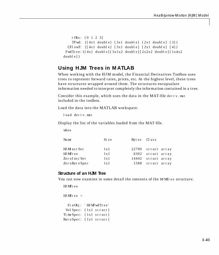
Using HJM Trees in MATLABWhen working with the HJM model, the Financial Derivatives Toolbox usestrees to represent forward rates, prices, etc. At the highest level, these treeshave structures wrapped around them. The structures encapsulateinformation needed to interpret completely the information contained in a tree.
Consider this example, which uses the data in the MAT-file deriv.matincluded in the toolbox.
Load the data into the MATLAB workspace.
load deriv.mat
Display the list of the variables loaded from the MAT-file.
whos
Name Size Bytes Class
HJMInstSet 1x1 22700 struct arrayHJMTree 1x1 6302 struct arrayZeroInstSet 1x1 14442 struct arrayZeroRateSpec 1x1 1588 struct array
Structure of an HJM TreeYou can now examine in some detail the contents of the HJMTree structure.
HJMTree
HJMTree =
FinObj: 'HJMFwdTree'VolSpec: [1x1 struct]
TimeSpec: [1x1 struct]RateSpec: [1x1 struct]
1 Tutorial
1-42
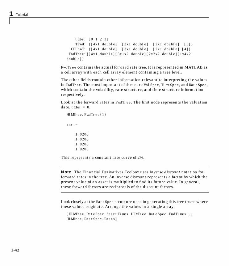
tObs: [0 1 2 3]TFwd: {[4x1 double] [3x1 double] [2x1 double] [3]}
CFlowT: {[4x1 double] [3x1 double] [2x1 double] [4]}FwdTree:{[4x1 double][3x1x2 double][2x2x2 double][1x4x2
double]}
FwdTree contains the actual forward rate tree. It is represented in MATLAB asa cell array with each cell array element containing a tree level.
The other fields contain other information relevant to interpreting the valuesin FwdTree. The most important of these are VolSpec, TimeSpec, and RateSpec,which contain the volatility, rate structure, and time structure informationrespectively.
Look at the forward rates in FwdTree. The first node represents the valuationdate, tObs = 0.
HJMTree.FwdTree{1}
ans =
1.0200 1.0200 1.0200 1.0200
This represents a constant rate curve of 2%.
Note The Financial Derivatives Toolbox uses inverse discount notation forforward rates in the tree. An inverse discount represents a factor by which thepresent value of an asset is multiplied to find its future value. In general,these forward factors are reciprocals of the discount factors.
Look closely at the RateSpec structure used in generating this tree to see wherethese values originate. Arrange the values in a single array.
[HJMTree.RateSpec.StartTimes HJMTree.RateSpec.EndTimes...HJMTree.RateSpec.Rates]

Heath-Jarrow-Morton (HJM) Model
1-43
ans =
0 1.0000 0.0200 1.0000 2.0000 0.0200 2.0000 3.0000 0.0200 3.0000 4.0000 0.0200
If you find the corresponding inverse discounts of the interest rates in the thirdcolumn, you have the values at the first node of the tree. You can turn interestrates into inverse discounts using the function rate2disc.
Disc = rate2disc(HJMTree.TimeSpec.Compounding,...HJMTree.RateSpec.Rates, HJMTree.RateSpec.EndTimes,...HJMTree.RateSpec.StartTimes);FRates = 1./Disc
FRates =1.0200
1.0200 1.0200 1.0200
The second node represents the first rate observation time, tObs = 1. This nodedisplays two states: one representing the branch going up and the otherrepresenting the branch going down.
Note that HJMTree.VolSpec.NumBranch = 2.
HJMTree.VolSpec
ans =
FinObj: 'HJMVolSpec' FactorModels: {'Constant'} FactorArgs: {{1x1 cell}} SigmaShift: 0 NumFactors: 1 NumBranch: 2 PBranch: [0.5000 0.5000] Fact2Branch: [-1 1]
Examine the rates of the node corresponding to the up branch.

1 Tutorial
1-44
HJMTree.FwdTree{2}(:,:,1)
ans =
0.9276 0.9368 0.9458
Now examine the corresponding down branch.
HJMTree.FwdTree{2}(:,:,2)
ans =
1.1329 1.1442 1.1552
The third node represents the second observation time, tObs = 2. This nodecontains a total of four states, two representing the branches going up and theother two representing the branches going down.
Examine the rates of the node corresponding to the up states.
HJMTree.FwdTree{3}(:,:,1)
ans =
0.8519 1.04050.8686 1.0609
Next examine the corresponding down states.
HJMTree.FwdTree{3}(:,:,2)
ans =
1.0405 1.27081.0609 1.2958
Starting at the third level, indexing within the tree cell array becomes complex,and isolating a specific node can be difficult. The function bushpath isolates aspecific node by specifying the path to the node as a vector of branches taken
Heath-Jarrow-Morton (HJM) Model
1-45
to reach that node. As an example, consider the node reached by starting fromthe root node, taking the branch up, then the branch down, and then anotherbranch down. Given that the tree has only two branches per node, branchesgoing up correspond to a 1, and branches going down correspond to a 2. Thepath up-down-down becomes the vector [1 2 2].
FRates = bushpath(HJMTree.FwdTree, [1 2 2])
FRates =
1.0200 0.9276 1.0405 1.1784
bushpath returns the spot rates for all the nodes touched by the path specifiedin the input argument, the first one corresponding to the root node, and the lastone corresponding to the target node.
Isolating the same node using direct indexing obtains
HJMTree.FwdTree{4}(:, 3, 2)
ans =
1.1784
As expected, this single value corresponds to the last element of the ratesreturned by bushpath.
You can use these techniques with any type of tree generated with theFinancial Derivatives Toolbox, such as forward rate trees or price trees.
Graphical View of Forward Rate TreeThe function treeviewer provides a graphical view of the path of forward ratesspecified in HJMTree. For example, here is a treeviewer representation of therates along both the up and the down branches of HJMTree.
1 Tutorial
1-46
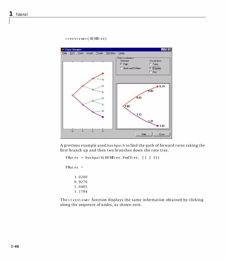
treeviewer(HJMTree)
A previous example used bushpath to find the path of forward rates taking thefirst branch up and then two branches down the rate tree.
FRates = bushpath(HJMTree.FwdTree, [1 2 2])
FRates =
1.0200 0.9276 1.0405 1.1784
The treeviewer function displays the same information obtained by clickingalong the sequence of nodes, as shown next.

Heath-Jarrow-Morton (HJM) Model
1-47
1 Tutorial
1-48
Pricing and Sensitivity from HJMThis section explains how to use the Financial Derivatives Toolbox to computeprices and sensitivities of several financial instruments using theHeath-Jarrow-Morton (HJM) model. For information, see:
• “Pricing and the Price Tree” on page 1-48 for a discussion of using thehjmprice function to compute prices for a portfolio of instruments.
• “Calculating Prices and Sensitivities” on page 1-61 for a discussion of usingthe hjmsens function to compute delta, gamma, and vega portfoliosensitivities.
Pricing and the Price TreeUsing the HJM model, the function that calculates the price of any set ofsupported instruments, based on an interest rate tree, is hjmprice. Thefunction is capable of pricing these instrument types:
• Bonds
• Bond options
• Arbitrary cash flows
• Fixed-rate notes
• Floating-rate notes
• Caps
• Floors
• Swaps
The syntax used for calling hjmprice is
[Price, PriceTree] = hjmprice(HJMTree, InstSet, Options)
This function requires two input arguments: the interest rate tree, HJMTree,and the set of instruments, InstSet. An optional argument Options furthercontrols the pricing and the output displayed.
HJMTree is the Heath-Jarrow-Morton tree sampling of a forward rate process,created using hjmtree. See “Building an HJM Forward Rate Tree” on page 1-35to learn how to create this structure based on the volatility model, the interestrate term structure, and the time layout.

Pricing and Sensitivity from HJM
1-49
InstSet is the set of instruments to be priced. This structure represents the setof instruments to be priced independently using the HJM model. The section“Creating and Managing Instrument Portfolios” on page 1-5 explains how tocreate this variable.
Options is an options structure created with the function derivset. Thisstructure defines how the HJM tree is used to find the price of instruments inthe portfolio, and how much additional information is displayed in thecommand window when the pricing function is called. If this input argument isnot specified in the call to hjmprice, a default Options structure is used.
In actuality, hjmprice is a wrapper function that classifies the instrumentsand calls appropriate pricing functions for each one of the instrument types.The calculation functions are bondbyhjm, cfbyhjm, fixedbyhjm, floatbyhjm,optbndbyhjm, and swapbyhjm. These functions may also be used directly tocalculate the price of sets of instruments of the same type. See thedocumentation for these individual functions for further information.
Consider the following example, which uses the data in the MAT-filederiv.mat included in the toolbox. Load the data into the MATLAB workspace.
load deriv.mat
Use the MATLAB whos command to display a list of the variables loaded fromthe MAT-file.
whos
Name Size Bytes Class
HJMInstSet 1x1 22700 struct arrayHJMTree 1x1 6302 struct arrayZeroInstSet 1x1 14442 struct arrayZeroRateSpec 1x1 1588 struct array
HJMTree and HJMInstSet are the input arguments needed to call the functionhjmprice.
Use the function instdisp to examine the set of instruments contained in thevariable HJMInstSet.
instdisp(HJMInstSet)

1 Tutorial
1-50
Note that there are eight instruments in this portfolio set: two bonds, one bondoption, one fixed rate note, one floating rate note, one cap, one floor, and oneswap. Each instrument has a corresponding index that identifies theinstrument prices in the price vector returned by hjmprice.
Now use hjmprice to calculate the price of each instrument in the instrumentset.
[Price, PriceTree] = hjmprice(HJMTree, HJMInstSet)Warning: Not all cash flows are aligned with the tree. Result willbe approximated.
Price =
105.7678107.6773
7.3217105.7678100.576815.436715.39385.1910
Index Type CouponRate Settle Maturity Period Basis ......... Name Quantity1 Bond 0.04 01-Jan-2000 01-Jan-2003 1 NaN......... 4% bond 1002 Bond 0.04 01-Jan-2000 01-Jan-2004 2 NaN......... 4% bond 50
Index Type UnderInd OptSpec Strike ExerciseDates AmericanOpt Name Quantity3 OptBond 2 call 101 01-Jan-2003 NaN Option 101 -50
Index Type CouponRate Settle Maturity FixedReset Basis Principal Name Quantity4 Fixed 0.04 01-Jan-2000 01-Jan-2003 1 NaN NaN 4% Fixed 80
Index Type Spread Settle Maturity FloatReset Basis Principal Name Quantity5 Float 20 01-Jan-2000 01-Jan-2003 1 NaN NaN 20BP Float 8
Index Type Strike Settle Maturity CapReset Basis Principal Name Quantity6 Cap 0.03 01-Jan-2000 01-Jan-2004 1 NaN NaN 3% Cap 30
Index Type Strike Settle Maturity FloorReset Basis Principal Name Quantity7 Floor 0.01 01-Jan-2000 01-Jan-2004 1 NaN NaN 1% Floor 40
Index Type LegRate Settle Maturity LegReset Basis Principal LegType Name Quantity8 Swap [0.04 20] 01-Jan-2000 01-Jan-2003 [1 1] NaN NaN [NaN] 4%/20BP Swap 10

Pricing and Sensitivity from HJM
1-51
PriceTree =
FinObj: 'HJMPriceTree'PBush: {1x5 cell}
AIBush: {1x5 cell}tObs: [0 1 2 3 4]
Note The warning shown above appears because some of the cash flows forthe second bond do not fall exactly on a tree node. This situation is discussedfurther in “HJM Pricing Options Structure” on page 1-56.
Price VectorThe prices in the vector Price correspond to the prices at observation time zero(tObs = 0), which is defined as the valuation date of the interest rate tree. Theinstrument indexing within the Price vector is the same as the indexing withinInstSet. In this example, the prices in the Price vector correspond to theinstruments in the following order.
InstNames = instget(HJMInstSet, 'FieldName','Name')
InstNames =
4% bond4% bondOption 1014% Fixed20BP Float3% Cap1% Floor4%/20BP Swap
Consequently, the price of the 3% cap is $15.4367, and the price for the 4%fixed-rate note is $105.7678
Price Tree StructureThe price tree structure holds all the pricing information. The first field of thisstructure, FinObj, indicates that this structure represents a price tree. The

1 Tutorial
1-52
second field, PBush is the tree holding the price of the instruments in each nodeof the tree. The third field, AIBush is the tree holding the accrued interest of theinstruments in each node of the tree. Finally, the fourth field, tObs, representsthe observation time of each level of PBush and AIBush, with units in terms ofcompounding periods.
The function treeviewer can obtain a graphical representation of the tree,allowing you to examine interactively the values on the nodes of the tree.
treeviewer(PriceTree, HJMInstSet)
Alternatively, you can directly examine the field within the PriceTreestructure, which contains the price tree with the price vectors at every state.The first node represents tObs = 0, corresponding to the valuation date.
PriceTree.PBush{1}
ans =
105.7678107.6773
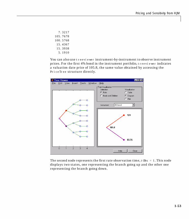
Pricing and Sensitivity from HJM
1-53
7.3217105.7678100.576815.436715.39385.1910
You can also use treeviewer instrument-by-instrument to observe instrumentprices. For the first 4% bond in the instrument portfolio, treeviewer indicatesa valuation date price of 105.8, the same value obtained by accessing thePriceTree structure directly.
The second node represents the first rate observation time, tObs = 1. This nodedisplays two states, one representing the branch going up and the other onerepresenting the branch going down.

1 Tutorial
1-54
Examine the prices of the node corresponding to the up branch.
PriceTree.PBush{2}(:,:,1)
ans =
124.0039135.237513.5026
124.0039100.4458
3.804230.409223.5581
As before, you can use treeviewer, this time to examine the price for the 4%bond on the up branch. treeviewer displays a price of 124 for the first node ofthe up branch, as expected.

Pricing and Sensitivity from HJM
1-55
Now examine the corresponding down branch
PriceTree.PBush{2}(:,:,2)
ans =
83.762376.38441.4337
83.7623100.330827.68670.9941
-16.5685
Use treeviewer once again, now to observe the price of the 4% bond on thedown branch. The displayed price of 83.76 conforms to the price obtained fromdirect access of the PriceTree structure. You may continue this process as faralong the price tree as you want.

1 Tutorial
1-56
HJM Pricing Options Structure
Default Structure. The HJM pricing Options structure defines how the HJM treeis used to find the price of instruments in the portfolio, and how muchadditional information is displayed in the command window when the pricingfunction is called. If this input argument is not specified in the call to hjmprice,a default Options structure is used.
To observe the default structure, use the derivset function without anyarguments.
Options = derivset
Options =
Diagnostics: 'off' Warnings: 'on' ConstRate: 'on'
As seen, the Options structure is composed of three fields: Diagnostics,Warnings, and ConstRate.
Diagnostics indicates whether additional information is displayed if the HJMtree is modified. The default value for this option is 'off'. If Diagnostics isset to 'on' and ConstRate is set to 'off', the pricing functions displayinformation such as the number of nodes in the last level of the HJM treegenerated for pricing purposes.
Warnings indicates whether to display warning messages when the input treeis not adequate for accurately pricing the instruments. The default value forthis option is 'on'. If both ConstRate and Warnings are 'on', a warning isdisplayed if any of the instruments in the input portfolio has a cash flow datebetween tree dates. If ConstRate is 'off', and Warnings is 'on', a warning isdisplayed if the tree is modified to match the cash flow dates on theinstruments in the portfolio.
ConstRate indicates whether the interest rates should be assumed constantbetween tree dates. By default this option is 'on', which is not anarbitrage-free assumption. Consequently the pricing functions return anapproximate price for instruments featuring cash flows between tree dates.Instruments featuring cash flows only on tree nodes are not affected by thisoption and return exact (arbitrage-free) prices. When ConstRate is 'off', the
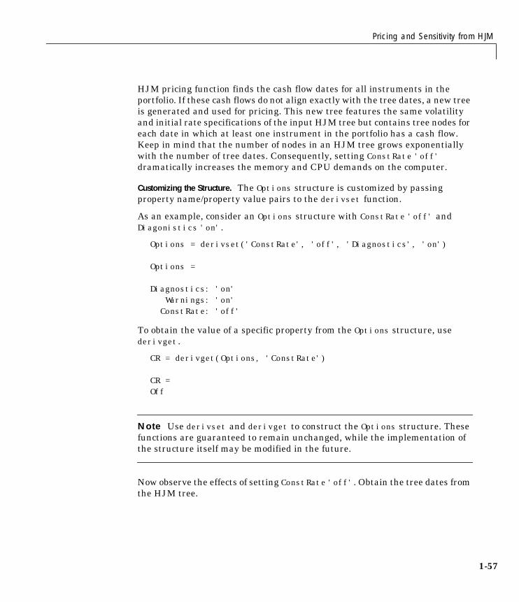
Pricing and Sensitivity from HJM
1-57
HJM pricing function finds the cash flow dates for all instruments in theportfolio. If these cash flows do not align exactly with the tree dates, a new treeis generated and used for pricing. This new tree features the same volatilityand initial rate specifications of the input HJM tree but contains tree nodes foreach date in which at least one instrument in the portfolio has a cash flow.Keep in mind that the number of nodes in an HJM tree grows exponentiallywith the number of tree dates. Consequently, setting ConstRate 'off'dramatically increases the memory and CPU demands on the computer.
Customizing the Structure. The Options structure is customized by passingproperty name/property value pairs to the derivset function.
As an example, consider an Options structure with ConstRate 'off' andDiagonistics 'on'.
Options = derivset('ConstRate', 'off', 'Diagnostics', 'on')
Options =
Diagnostics: 'on'Warnings: 'on'ConstRate: 'off'
To obtain the value of a specific property from the Options structure, usederivget.
CR = derivget(Options, 'ConstRate')
CR =Off
Note Use derivset and derivget to construct the Options structure. Thesefunctions are guaranteed to remain unchanged, while the implementation ofthe structure itself may be modified in the future.
Now observe the effects of setting ConstRate 'off'. Obtain the tree dates fromthe HJM tree.

1 Tutorial
1-58
TreeDates = [HJMTree.TimeSpec.ValuationDate;...HJMTree.TimeSpec.Maturity]
TreeDates =
730486730852731217731582731947
datedisp(TreeDates)
01-Jan-200001-Jan-200101-Jan-200201-Jan-200301-Jan-2004
All instruments in HJMInstSet settle on Jan 1st, 2000, and all have cash flowsonce a year, with the exception of the second bond, which features a period of2. This bond has cash flows twice a year, with every other cash flowconsequently falling between tree dates. You can extract this bond from theportfolio to compare how its price differs by setting ConstRate to 'on' and'off'.
BondPort = instselect(HJMInstSet, 'Index', 2);
instdisp(BondPort)
Index Type CouponRate Settle Maturity Period Basis...1 Bond 0.04 01-Jan-2000 01-Jan-2004 2 NaN...
First price the bond with ConstRate 'on' (default).
format long[BondPrice, BondPriceTree] = hjmprice(HJMTree, BondPort)Warning: Not all cash flows are aligned with the tree. Result willbe approximated.
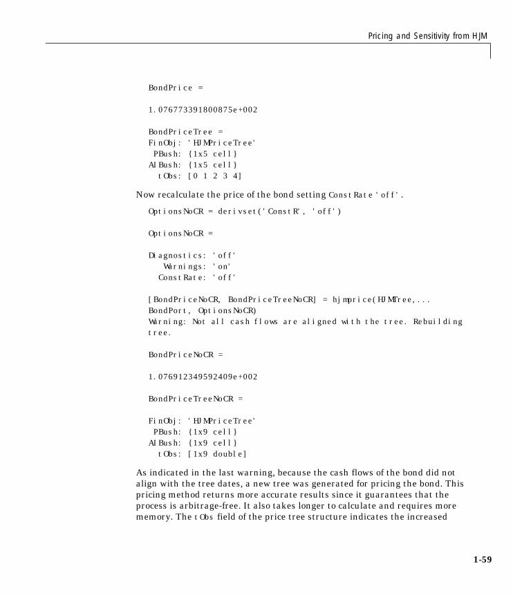
Pricing and Sensitivity from HJM
1-59
BondPrice =
1.076773391800875e+002
BondPriceTree =FinObj: 'HJMPriceTree'PBush: {1x5 cell}
AIBush: {1x5 cell}tObs: [0 1 2 3 4]
Now recalculate the price of the bond setting ConstRate 'off'.
OptionsNoCR = derivset('ConstR', 'off')
OptionsNoCR =
Diagnostics: 'off'Warnings: 'on'ConstRate: 'off'
[BondPriceNoCR, BondPriceTreeNoCR] = hjmprice(HJMTree,...BondPort, OptionsNoCR)Warning: Not all cash flows are aligned with the tree. Rebuildingtree.
BondPriceNoCR =
1.076912349592409e+002
BondPriceTreeNoCR =
FinObj: 'HJMPriceTree'PBush: {1x9 cell}
AIBush: {1x9 cell}tObs: [1x9 double]
As indicated in the last warning, because the cash flows of the bond did notalign with the tree dates, a new tree was generated for pricing the bond. Thispricing method returns more accurate results since it guarantees that theprocess is arbitrage-free. It also takes longer to calculate and requires morememory. The tObs field of the price tree structure indicates the increased

1 Tutorial
1-60
memory usage. BondPriceTree.tObs has only five elements, whileBondPriceTreeNoCR has nine. While this may not seem like a large difference,it has a dramatic effect on the number of states in the last node.
size(BondPriceTree.PBush{end})
ans =
1 8
size(BondPriceTreeNoCR.PBush{end})
ans =
1 128
The differences become more obvious by examining the price trees withtreeviewer.
treeviewer(BondPriceTree, BondPort)

Pricing and Sensitivity from HJM
1-61
treeviewer(BondPriceTreeNoCR, BondPort)
Calculating Prices and SensitivitiesThe function hjmsens computes the delta, gamma, and vega sensitivities ofinstruments using an interest rate tree created with hjmtree. It also optionallyreturns the calculated price for each instrument. hjmsens requires the sametwo input arguments used by hjmprice, namely HJMTree and InstSet.
hjmsens calculates the dollar value of delta and gamma by shifting theobserved forward yield curve by 100 basis points in each direction, and thedollar value of vega by shifting the volatility process by 1%. To obtain theper-dollar value of the sensitivities, divide the dollar sensitivity by the price ofthe corresponding instrument.
The calling syntax for the function is
[Delta, Gamma, Vega, Price] = hjmsens(HJMTree, HJMInstSet)

1 Tutorial
1-62
Use the previous example data to calculate the price of instruments.
load deriv.mat[Delta, Gamma, Vega, Price] = hjmsens(HJMTree, HJMInstSet);Warning: Not all cash flows are aligned with the tree. Result willbe approximated.
Note The warning appears because some of the cash flows for the secondbond do not fall exactly on a tree node. This situation was discussed in “HJMPricing Options Structure” on page 1-56.
The sensitivities and the prices can be examined conveniently by arrangingthem into a single matrix.
All = [Delta, Gamma, Vega, Price]
All =
1.0e+003 *
-0.2997 1.1603 -0.0000 0.1058 -0.3958 1.9012 -0.0003 0.1077 -0.0818 0.5566 0.0610 0.0073 -0.2997 1.1603 -0.0000 0.1058 -0.0011 0.0037 0 0.1006 0.1085 -0.6975 0.1665 0.0154 -0.1741 0.9569 0.1615 0.0154 -0.2986 1.1567 -0.0000 0.0052
As with the prices, each row of the sensitivity vectors corresponds to thesimilarly indexed instrument in HJMInstSet. To view the per-dollarsensitivities, divide each dollar sensitivity by the corresponding instrumentprice.

Pricing and Sensitivity from HJM
1-63
All = [Delta ./ Price, Gamma ./ Price, Vega ./ Price, Price]
All =
-2.8337 10.9706 -0.0000 105.7678 -3.6759 17.6566 -0.0026 107.6773 -11.1729 76.0234 8.3312 7.3217 -2.8337 10.9706 -0.0000 105.7678 -0.0112 0.0364 0 100.5768 7.0273 -45.1870 10.7873 15.4367 -11.3117 62.1593 10.4911 15.3938 -57.5215 222.8243 -0.0000 5.1910
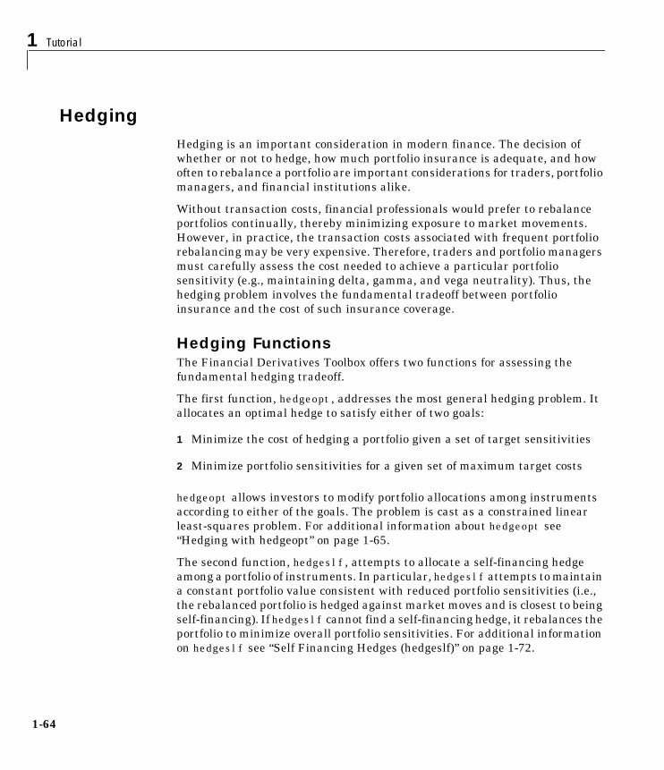
1 Tutorial
1-64
HedgingHedging is an important consideration in modern finance. The decision ofwhether or not to hedge, how much portfolio insurance is adequate, and howoften to rebalance a portfolio are important considerations for traders, portfoliomanagers, and financial institutions alike.
Without transaction costs, financial professionals would prefer to rebalanceportfolios continually, thereby minimizing exposure to market movements.However, in practice, the transaction costs associated with frequent portfoliorebalancing may be very expensive. Therefore, traders and portfolio managersmust carefully assess the cost needed to achieve a particular portfoliosensitivity (e.g., maintaining delta, gamma, and vega neutrality). Thus, thehedging problem involves the fundamental tradeoff between portfolioinsurance and the cost of such insurance coverage.
Hedging FunctionsThe Financial Derivatives Toolbox offers two functions for assessing thefundamental hedging tradeoff.
The first function, hedgeopt, addresses the most general hedging problem. Itallocates an optimal hedge to satisfy either of two goals:
1 Minimize the cost of hedging a portfolio given a set of target sensitivities
2 Minimize portfolio sensitivities for a given set of maximum target costs
hedgeopt allows investors to modify portfolio allocations among instrumentsaccording to either of the goals. The problem is cast as a constrained linearleast-squares problem. For additional information about hedgeopt see“Hedging with hedgeopt” on page 1-65.
The second function, hedgeslf, attempts to allocate a self-financing hedgeamong a portfolio of instruments. In particular, hedgeslf attempts to maintaina constant portfolio value consistent with reduced portfolio sensitivities (i.e.,the rebalanced portfolio is hedged against market moves and is closest to beingself-financing). If hedgeslf cannot find a self-financing hedge, it rebalances theportfolio to minimize overall portfolio sensitivities. For additional informationon hedgeslf see “Self Financing Hedges (hedgeslf)” on page 1-72.

Hedging
1-65
Hedging with hedgeoptTo illustrate the hedging functions, consider the delta, gamma, and vegasensitivity measures. In the context of the Financial Derivatives Toolbox, deltais the price sensitivity measure of shifts in the forward yield curve, gamma isthe delta sensitivity measure of shifts in the forward yield curve, and vega isthe price sensitivity measure of shifts in the volatility process. Note that thedelta, gamma, and vega sensitivities calculated by the toolbox are dollarsensitivities. (See “Calculating Prices and Sensitivities” on page 1-61 fordetails.)
Note The numerical results in this section are displayed with the MATLABbank format. Although the calculations are performed in floating-point doubleprecision, only two decimal places are displayed.
To illustrate the hedging facility, consider the portfolio HJMInstSet obtainedfrom the example file deriv.mat. The portfolio consists of eight instruments:two bonds, one bond option, one fixed rate note, one floating rate note, one cap,one floor, and one swap.
Both hedging functions require some common inputs, including the currentportfolio holdings (allocations), and a matrix of instrument sensitivities. Loadthe portfolio into memory
load deriv.mat;
compute price and sensitivities
[Delta, Gamma, Vega, Price] = hjmsens(HJMTree, HJMInstSet);Warning: Not all cash flows are aligned with the tree. Result willbe approximated.
and extract the current portfolio holdings.
Holdings = instget(HJMInstSet, 'FieldName', 'Quantity');
For convenience place the delta, gamma, and vega sensitivity measures into amatrix of sensitivities.
Sensitivities = [Delta Gamma Vega];

1 Tutorial
1-66
Each row of the Sensitivities matrix is associated with a differentinstrument in the portfolio, and each column with a different sensitivitymeasure.
To summarize the portfolio information
disp([Price Holdings Sensitivities])
105.77 100.00 -299.72 1160.34 -0.00107.68 50.00 -395.81 1901.22 -0.287.32 -50.00 -81.80 556.62 61.00
105.77 80.00 -299.72 1160.34 -0.00100.58 8.00 -1.12 3.66 015.44 30.00 108.48 -697.54 166.5215.39 40.00 -174.13 956.87 161.505.19 10.00 -298.59 1156.68 -0.00
The first column above is the dollar unit price of each instrument, the secondis the holdings of each instrument (the quantity held or the number ofcontracts), and the third, fourth, and fifth columns are the dollar delta, gamma,and vega sensitivities, respectively.
The current portfolio sensitivities are a weighted average of the instruments inthe portfolio.
TargetSens = Holdings' * Sensitivities
TargetSens = -76355.34 305035.28 8391.37
Maintaining Existing AllocationsTo illustrate using hedgeopt, suppose that you want to maintain your existingportfolio. The first form of hedgeopt minimizes the cost of hedging a portfoliogiven a set of target sensitivities. If you want to maintain your existingportfolio composition and exposure, you should be able to do so withoutspending any money. To verify this, set the target sensitivities to the currentsensitivities.

Hedging
1-67
[Sens, Cost, Quantity] = hedgeopt(Sensitivities, Price,...Holdings, [], [], [], TargetSens);
Sens = -76355.34 305035.28 8391.37
Cost = 0
Quantity' = 100.00 50.00 -50.00 80.00 8.00 30.00 40.00 10.00
Note that our portfolio composition and sensitivities are unchanged and thatthe cost associated with doing nothing is zero. The cost is defined as the changein portfolio value. This number cannot be less than zero because therebalancing cost is defined as a nonnegative number.
If Value0 and Value1 represent the portfolio value before and afterrebalancing, respectively, the zero cost can also be verified by comparing theportfolio values.
Value0 = Holdings' * Price
Value0 = 25991.36
Value1 = Quantity * Price
Value1 = 25991.36
Partially Hedged PortfolioBuilding upon the previous example, suppose you want to know the cost toachieve an overall portfolio dollar sensitivity of [-23000 -3300 3000], while

1 Tutorial
1-68
allowing trading only in instruments 2, 3, and 6 (holding the positions ofinstruments 1, 4, 5, 7, and 8 fixed.) To find the cost, first set the target portfoliodollar sensitivity.
TargetSens = [-23000 -3300 3000];
Then, specify the instruments to be fixed.
FixedInd = [1 4 5 7 8];
Finally, call hedgeopt
[Sens, Cost, Quantity] = hedgeopt(Sensitivities, Price, ...Holdings, FixedInd,[], [], TargetSens);
and again examine the results
Sens = -23000.00 -3300.00 3000.00
Cost = 8029.28
Quantity' = 100.00 -15.99 -303.08 80.00 8.00 90.22 40.00 10.00
Recompute Value1, the portfolio value after rebalancing.
Value1 = Quantity * Price
Value1 = 17962.08
As expected, the cost, $8,029.28, is the difference between Value0 and Value1,$25,991.36 - $17,962.08. Only the positions in instruments 2, 3, and 6 havebeen changed.

Hedging
1-69
Fully Hedged PortfolioThe above example illustrates a partial hedge, but perhaps the mostinteresting case involves the cost associated with a fully-hedged portfolio(simultaneous delta, gamma, and vega neutrality). In this case, set the targetsensitivity to a row vector of zeros and call hedgeopt again.
TargetSens = [0 0 0];[Sens, Cost, Quantity] = hedgeopt(Sensitivities, Price, ...Holdings, FixedInd,[], [], TargetSens);
Examining the outputs, you obtain a fully-hedged portfolio
Sens = -0.00 0.00 0.00
but at an expense of over $30,000,
Cost = 30310.85
The positions needed to achieve a fully-hedged portfolio
Quantity' = 100.00 -227.78 181.00 80.00 8.00 -105.49 40.00 10.00
result in a negative portfolio value.
Value1 = Quantity * Price
Value1 = -4319.49
Minimizing Portfolio SensitivitiesThe above examples illustrate how to use hedgeopt to determine the minimumcost of hedging a portfolio given a set of target sensitivities. In these examples,portfolio target sensitivities are treated as equality constraints during the
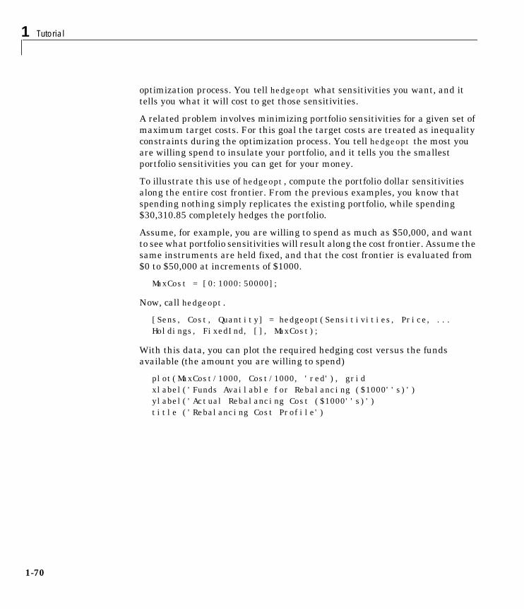
1 Tutorial
1-70
optimization process. You tell hedgeopt what sensitivities you want, and ittells you what it will cost to get those sensitivities.
A related problem involves minimizing portfolio sensitivities for a given set ofmaximum target costs. For this goal the target costs are treated as inequalityconstraints during the optimization process. You tell hedgeopt the most youare willing spend to insulate your portfolio, and it tells you the smallestportfolio sensitivities you can get for your money.
To illustrate this use of hedgeopt, compute the portfolio dollar sensitivitiesalong the entire cost frontier. From the previous examples, you know thatspending nothing simply replicates the existing portfolio, while spending$30,310.85 completely hedges the portfolio.
Assume, for example, you are willing to spend as much as $50,000, and wantto see what portfolio sensitivities will result along the cost frontier. Assume thesame instruments are held fixed, and that the cost frontier is evaluated from$0 to $50,000 at increments of $1000.
MaxCost = [0:1000:50000];
Now, call hedgeopt.
[Sens, Cost, Quantity] = hedgeopt(Sensitivities, Price, ...Holdings, FixedInd, [], MaxCost);
With this data, you can plot the required hedging cost versus the fundsavailable (the amount you are willing to spend)
plot(MaxCost/1000, Cost/1000, 'red'), gridxlabel('Funds Available for Rebalancing ($1000''s)')ylabel('Actual Rebalancing Cost ($1000''s)')title ('Rebalancing Cost Profile')

Hedging
1-71
Figure 1-1: Rebalancing Cost Profile
and the portfolio dollar sensitivities versus the funds available
figureplot(MaxCost/1000, Sens(:,1), '-red')hold('on')plot(MaxCost/1000, Sens(:,2), '-.black')plot(MaxCost/1000, Sens(:,3), '--blue')gridxlabel('Funds Available for Rebalancing ($1000''s)')ylabel('Delta, Gamma, and Vega Portfolio Dollar Sensitivities')title ('Portfolio Sensitivities Profile')legend('Delta', 'Gamma', 'Vega', 0)

1 Tutorial
1-72
Figure 1-2: Funds Available for Rebalancing
Self Financing Hedges (hedgeslf)Figure 1-1 and Figure 1-2 indicate that there is no benefit to be gained becausethe funds available for hedging exceed $30,310.85, the point of maximumexpense required to obtain simultaneous delta, gamma, and vega neutrality.You can also find this point of delta, gamma, and vega neutrality fromhedgeslf.
[Sens, Value1, Quantity] = hedgeslf(Sensitivities, Price,...Holdings, FixedInd);
Sens = -0.00 0.00 0.00Value1 = -4319.49

Hedging
1-73
Quantity = 100.00 -227.78 181.00 80.00 8.00 -105.49 40.00 10.00
Similar to hedgeopt, hedgeslf returns the portfolio dollar sensitivities andinstrument quantities (the rebalanced holdings). However, in contrast, thesecond output parameter of hedgeslf is the value of the rebalanced portfolio,from which you can calculate the rebalancing cost by subtraction.
Value0 - Value1
ans = 30310.85
In our example, the portfolio is clearly not self-financing, so hedgeslf finds thebest possible solution required to obtain zero sensitivities.
There is, in fact, a third calling syntax available for hedgeopt directly relatedto the results shown above for hedgeslf. Suppose, instead of directly specifyingthe funds available for rebalancing (the most money you are willing to spend),you want to simply specify the number of points along the cost frontier. Thiscall to hedgeopt samples the cost frontier at 10 equally-spaced points betweenthe point of minimum cost (and potentially maximum exposure) and the pointof minimum exposure (and maximum cost).
[Sens, Cost, Quantity] = hedgeopt(Sensitivities, Price,...Holdings, FixedInd, 10);
Sens = -31259.69 -4609.41 4161.86 -27786.39 -4097.25 3699.43 -24313.09 -3585.09 3237.00 -20839.79 -3072.94 2774.57 -17366.49 -2560.78 2312.14 -13893.19 -2048.63 1849.71 -10419.90 -1536.47 1387.29

1 Tutorial
1-74
-6946.60 -1024.31 924.86 -3473.30 -512.16 462.43 -0.00 -0.00 -0.00Cost = 0 3367.87 6735.74 10103.62 13471.49 16839.36 20207.23 23575.10 26942.98 30310.85
Now plot this data.
figureplot(Cost/1000, Sens(:,1), '-red')hold('on')plot(Cost/1000, Sens(:,2), '-.black')plot(Cost/1000, Sens(:,3), '--blue')gridxlabel('Rebalancing Cost ($1000''s)')ylabel('Delta, Gamma, and Vega Portfolio Dollar Sensitivities')title ('Portfolio Sensitivities Profile')legend('Delta', 'Gamma', 'Vega', 0)

Hedging
1-75
Figure 1-3: Rebalancing Cost
In this calling form, hedgeopt calls hedgeslf internally to determine themaximum cost needed to minimize the portfolio sensitivities ($30,310.85), andevenly samples the cost frontier between $0 and $30,310.85.
Note that both hedgeopt and hedgeslf cast the optimization problem as aconstrained linear least-squares problem. Depending upon the instrumentsand constraints, neither function is guaranteed to converge to a solution. Insome cases, the problem space may unbounded, and additional instrumentequality constraints, or user-specified constraints, may be necessary forconvergence. See “Hedging with Constrained Portfolios” on page 1-79 foradditional information.
Specifying Constraints with ConSetBoth hedgeopt and hedgeslf accept an optional input argument, ConSet, thatallows you to specify a set of linear inequality constraints for instruments inyour portfolio. The examples in this section are quite brief. For additionalinformation regarding portfolio constraint specifications, refer to the section“Analyzing Portfolios” found in the Financial Toolbox User's Guide.

1 Tutorial
1-76
For the first example of setting constraints, return to the fully-hedged portfolioexample that used hedgeopt to determine the minimum cost of obtainingsimultaneous delta, gamma, and vega neutrality (target sensitivities all zero).Recall that when hedgeopt computes the cost of rebalancing a portfolio, theinput target sensitivities you specify are treated as equality constraints duringthe optimization process. The situation is reproduced below for convenience.
TargetSens = [0 0 0];[Sens, Cost, Quantity] = hedgeopt(Sensitivities, Price,...Holdings, FixedInd, [], [], TargetSens);
The outputs provide a fully-hedged portfolio
Sens = -0.00 0.00 0.00
at an expense of over $30,000.
Cost = 30310.85
The positions needed to achieve this fully-hedged portfolio are
Quantity' = 100.00 -227.78 181.00 80.00 8.00 -105.49 40.00 10.00
Suppose now that you want to place some upper and lower bounds on theindividual instruments in your portfolio. You can specify these constraints,along with a variety of general linear inequality constraints, with the FinancialToolbox function portcons.
As an example, assume that, in addition to holding instruments 1, 4, 5, 7, and8 fixed as before, you want to bound the position of all instruments to within +/- 200 contracts (for each instrument, you cannot short or long more than 200contracts). Applying these constraints disallows the current position in the

Hedging
1-77
second instrument (short 227.78). All other instruments are currently withinthe upper/lower bounds.
You can generate these constraints by first specifying the lower and upperbounds vectors and then calling portcons.
LowerBounds = [-200 -200 -200 -200 -200 -200 -200 -200];UpperBounds = [ 200 200 200 200 200 200 200 200];ConSet = portcons('AssetLims', LowerBounds, UpperBounds);
To impose these constraints, call hedgeopt with ConSet as the last input.
[Sens, Cost, Quantity] = hedgeopt(Sensitivities, Price,...Holdings, FixedInd, [], [], TargetSens, ConSet);
Examine the outputs and see that they are all set to NaN, indicating that theproblem, given the constraints, is not solvable. Intuitively, the results meanthat you cannot obtain simultaneous delta, gamma, and vega neutrality withthese constraints at any price.
To see how close you can get to portfolio neutrality with these constraints, callhedgeslf.
[Sens, Value1, Quantity] = hedgeslf(Sensitivities, Price,...Holdings, FixedInd, ConSet);
Sens = -3021.91 -452.25 74.17
Value1 = -1429.15
Quantity = 100.00 -200.00 115.83 80.00 8.00 -81.12 40.00 10.00

1 Tutorial
1-78
hedgeslf enforces the lower bound for the second instrument, but thesensitivity is far from neutral. The cost to obtain this portfolio is
Value0 - Value1
ans = 27420.51
As a final example of user-specified constraints, rebalance the portfolio usingthe second hedging goal of hedgeopt. Assume that you are willing to spend asmuch as $20,000 to rebalance your portfolio, and you want to know whatminimum portfolio sensitivities you can get for your money. In this form, recallthat the target cost ($20,000) is treated as an inequality constraint during theoptimization process.
For reference, invoke hedgeopt without any user-specified linear inequalityconstraints.
[Sens, Cost, Quantity] = hedgeopt(Sensitivities, Price,...Holdings, FixedInd, [], 20000);
Sens = -10633.62 -1567.98 1415.74
Cost = 20000.00
Quantity' = 100.00 -129.80 -42.85 80.00 8.00 -14.82 40.00 10.00
This result corresponds to the $20,000 point along the Portfolio SensitivitiesProfile shown in Figure 1-3, Rebalancing Cost, on page 1-75.
Assume that, in addition to holding instruments 1, 4, 5, 7, and 8 fixed as before,you wish to bound the position of all instruments to within +/- 120 contracts (for

Hedging
1-79
each instrument, you cannot short more than 120 contracts and you cannotlong more than 120 contracts). These bounds disallow the current position inthe second instrument (-129.80). All other instruments are currently withinthe upper/lower bounds.
As before, you can generate these constraints by first specifying the lower andupper bounds vectors and then calling portcons.
LowerBounds = [-120 -120 -120 -120 -120 -120 -120 -120];UpperBounds = [ 120 120 120 120 120 120 120 120];ConSet = portcons('AssetLims', LowerBounds, UpperBounds);
To impose these constraints, again call hedgeopt with ConSet as the last input.
[Sens, Cost, Quantity] = hedgeopt(Sensitivities, Price,...Holdings,FixedInd, [], 20000, [], ConSet);
Sens = -11724.04 -1754.57 287.75
Cost = 19097.25
Quantity' = 100.00 -120.00 -71.83 80.00 8.00 -10.96 40.00 10.00
With these constraints hedgeopt enforces the lower bound for the secondinstrument. The cost incurred is $19,097.25.
Hedging with Constrained PortfoliosBoth hedging functions cast the optimization as a constrained linear leastsquares problem. (See the function lsqlin in the Optimization Toolbox fordetails.) In particular, lsqlin attempts to minimize the constrained linearleast squares problem
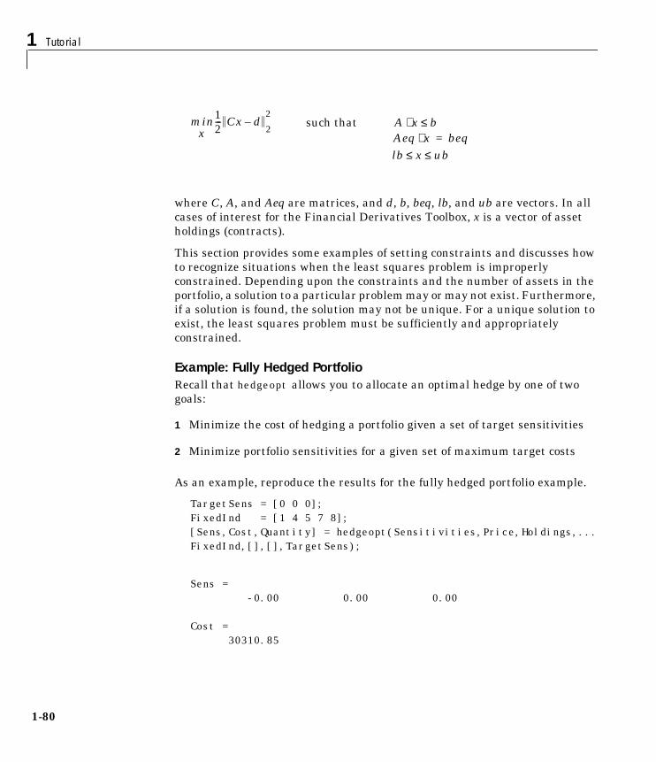
1 Tutorial
1-80
where C, A, and Aeq are matrices, and d, b, beq, lb, and ub are vectors. In allcases of interest for the Financial Derivatives Toolbox, x is a vector of assetholdings (contracts).
This section provides some examples of setting constraints and discusses howto recognize situations when the least squares problem is improperlyconstrained. Depending upon the constraints and the number of assets in theportfolio, a solution to a particular problem may or may not exist. Furthermore,if a solution is found, the solution may not be unique. For a unique solution toexist, the least squares problem must be sufficiently and appropriatelyconstrained.
Example: Fully Hedged PortfolioRecall that hedgeopt allows you to allocate an optimal hedge by one of twogoals:
1 Minimize the cost of hedging a portfolio given a set of target sensitivities
2 Minimize portfolio sensitivities for a given set of maximum target costs
As an example, reproduce the results for the fully hedged portfolio example.
TargetSens = [0 0 0];FixedInd = [1 4 5 7 8];[Sens,Cost,Quantity] = hedgeopt(Sensitivities,Price,Holdings,...FixedInd,[],[],TargetSens);
Sens = -0.00 0.00 0.00
Cost = 30310.85
min12--- Cx d–
2
2
xsuch that A x⋅ b≤
Aeq x⋅ beq=
lb x ub≤ ≤

Hedging
1-81
Quantity' = 100.00 -227.78 181.00 80.00 8.00 -105.49 40.00 10.00
This example finds a unique solution at a cost of just over $30,310. The matrixC (formed internally by hedgeopt and passed to lsqlin) is the asset Pricevector expressed as a row vector.
C = Price' = [105.77 107.68 7.32 105.77 100.58 15.44 15.39 5.19]
The vector d is the current portfolio value Value0 = 25991.36. The examplemaintains, as closely as possible, a constant portfolio value subject to thespecified constraints.
Additional Constraints. In the absence of any additional constraints, the leastsquares objective involves a single equation with eight unknowns. This is anunder-determined system of equations. Because such systems generally havean infinite number of solutions, you need to specify additional constraints toachieve a solution with practical significance. The additional constraints cancome from two sources:
• User-specified equality constraints
• Target sensitivity equality constraints imposed by hedgeopt
The fully-hedged portfolio example specifies five equality constraintsassociated with holding assets 1, 4, 5, 7, and 8 fixed. This reduces the numberof unknowns from eight to three, which is still an under-determined system.However, when combined with the first goal of hedgeopt, the equalityconstraints associated with the target sensitivities in TargetSens produce anadditional system of three equations with three unknowns. This additionalsystem guarantees that the weighted average of the delta, gamma, and vega ofassets 2, 3, and 6, together with the remaining assets held fixed, satisfy theoverall portfolio target sensitivity requirements in TargetSens.
Combining the least squares objective equation with the three portfoliosensitivity equations provides an overall system of four equations with three

1 Tutorial
1-82
unknown asset holdings. This is no longer an under-determined system, andthe solution is as shown.
If the assets held fixed are reduced, e.g., FixedInd = [1 4 5 7], hedgeoptreturns a no cost, fully-hedged portfolio (Sens = [0 0 0] and Cost = 0).
If you further reduce FixedInd (e.g., [1 4 5], [1 4], or even []), hedgeoptalways returns a no cost, fully-hedged portfolio. In these cases, insufficientconstraints result in an under-determined system. Although hedgeoptidentifies no cost, fully-hedged portfolios, there is nothing unique about them.These portfolios have little practical significance.
Constraints must be sufficient and appropriately defined. Additionalconstraints having no effect on the optimization are called dependentconstraints. As a simple example, assume that parameter Z is constrained suchthat . Furthermore, assume we somehow add another constraint thateffectively restricts . The constraint now has no effect on theoptimization.
Example: Minimize Portfolio SensitivitiesTo illustrate using hedgeopt to minimize portfolio sensitivities for a givenmaximum target cost, specify a target cost of $20,000 and determine the newportfolio sensitivities, holdings, and cost of the rebalanced portfolio.
MaxCost = 20000;[Sens, Cost, Quantity] = hedgeopt(Sensitivities, Price,...Holdings, [1 4 5 7 8], [], MaxCost);
Sens = -10633.62 -1567.98 1415.74
Cost = 20000.00
Quantity' = 100.00 -129.80 -42.85 80.00 8.00 -14.82
Z 1≤Z 0≤ Z 1≤

Hedging
1-83
40.00 10.00
This example corresponds to the $20,000 point along the cost axis inFigure 1-1, Figure 1-2, and Figure 1-3.
When minimizing sensitivities, the maximum target cost is treated as aninequality constraint; in this case, MaxCost is the most you are willing to spendto hedge a portfolio. The least squares objective matrix C is the matrixtranspose of the input asset sensitivities
C = Sensitivities'
a 3-by-8 matrix in this example, and d is a 3-by-1 column vector of zeros,[0 0 0]'.
Without any additional constraints, the least squares objective results in anunder-determined system of three equations with eight unknowns. By holdingassets 1, 4, 5, 7, and 8 fixed, you reduce the number of unknowns from eight tothree. Now, with a system of three equations with three unknowns, hedgeoptfinds the solution shown.
Example: Under-Determined SystemReducing the number of assets held fixed creates an under-determined systemwith meaningless solutions. For example, see what happens with only fourassets constrained.
FixedInd = [1 4 5 7];
[Sens, Cost, Quantity] = hedgeopt(Sensitivities, Price,...Holdings, FixedInd, [], MaxCost)
Sens = -0.00 0.00 0.00
Cost = 20000.00

1 Tutorial
1-84
Quantity' =100.00
-126.00 71.43 80.00 8.00 -65.17 40.00 -80.25
You have spent $20,000 (all the funds available for rebalancing) to achieve afully-hedged portfolio.
With an increase in available funds to $50,000, you still spend all availablefunds to get another fully-hedged portfolio.
MaxCost = 50000;[Sens, Cost, Quantity] = hedgeopt(Sensitivities, Price, Holdings,FixedInd , [],MaxCost);
Sens = -0.00 0.00 0.00
Cost = 50000.00
Quantity' = 100.00 -422.13 390.24 80.00 8.00 -182.46 40.00 182.34
All solutions to an under-determined system are meaningless. You buy and sellvarious assets to obtain zero sensitivities, spending all available funds everytime. If you reduce the number of fixed assets any further, this problem isinsufficiently constrained, and you find no solution (the outputs are all NaN).

Hedging
1-85
Note also that no solution exists whenever constraints are inconsistent.Inconsistent constraints create an infeasible solution space; the outputs are allNaN.
Portfolio Constraints with hedgeslfThe other hedging function, hedgeslf, attempts to minimize portfoliosensitivities such that the rebalanced portfolio maintains a constant value (therebalanced portfolio is hedged against market moves and is closest to beingself-financing). If a self-financing hedge is not found, hedgeslf tries torebalance a portfolio to minimize sensitivities.
From a least squares systems approach, hedgeslf first attempts to minimizecost in the same way that hedgeopt does. If it cannot solve this problem (a nocost, self-financing hedge is not possible), hedgeslf proceeds to minimizesensitivities like hedgeopt. Thus, the discussion of constraints for hedgeopt isdirectly applicable to hedgeslf as well.

1 Tutorial
1-86
2
Function Reference
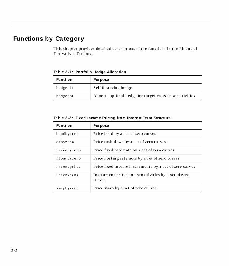
2-2
Functions by CategoryThis chapter provides detailed descriptions of the functions in the FinancialDerivatives Toolbox.
Table 2-1: Portfolio Hedge Allocation
Function Purpose
hedgeslf Self-financing hedge
hedgeopt Allocate optimal hedge for target costs or sensitivities
Table 2-2: Fixed Income Pricing from Interest Term Structure
Function Purpose
bondbyzero Price bond by a set of zero curves
cfbyzero Price cash flows by a set of zero curves
fixedbyzero Price fixed rate note by a set of zero curves
floatbyzero Price floating rate note by a set of zero curves
intenvprice Price fixed income instruments by a set of zero curves
intenvsens Instrument prices and sensitivities by a set of zerocurves
swapbyzero Price swap by a set of zero curves

2-3
Table 2-3: Fixed Income Pricing and Sensitivity from Heath-Jarrow-MortonTree
Function Purpose
hjmprice Fixed income instrument prices by HJM interest ratetree
hjmsens Fixed income instrument price and sensitivities byHJM interest rate tree
hjmtimespec Specify time structure for HJM interest rate tree
hjmtree Construct HJM interest rate tree
hjmvolspec Volatility process specification
Table 2-4: Heath-Jarrow-Morton Utilities
Function Purpose
bondbyhjm Price bond by HJM interest rate tree
capbyhjm Price cap by HJM interest rate tree
cfbyhjm Price arbitrary set of cash flows by HJM interest ratetree
fixedbyhjm Price fixed rate note by HJM interest rate tree
floatbyhjm Price floating rate note by HJM interest rate tree
floorbyhjm Price floor by HJM interest rate tree
mmktbyhjm Create money market tree
optbndbyhjm Price bond option by HJM interest rate tree
swapbyhjm Price swap by HJM interest rate tree

2-4
Table 2-5: Heath-Jarrow-Morton Bushy Tree Manipulation
Function Purpose
bushpath Extract entries from node of bushy tree
bushshape Retrieve shape of bushy tree
mkbush Create bushy tree
treeviewer Display Heath-Jarrow-Morton (HJM) tree
Table 2-6: Heath-Jarrow-Morton Derivatives Pricing Options
Function Purpose
derivget Get derivatives pricing options
derivset Set or modify derivatives pricing options
Table 2-7: Instrument Portfolio Handling
Function Purpose
instadd Add types to instrument collection
instaddfield Add new instruments to an instrument collection
instbond Construct bond instrument
instcap Construct cap instrument
instcf Constructor for arbitrary cash flow instrument
instdelete Complement of subset of instruments by matchingconditions
instdisp Display instruments

2-5
instfields List fieldnames
instfind Search instruments for matching conditions
instfixed Construct fixed-rate instrument
instfloat Construct floating-rate instrument
instfloor Construct floor instrument
instget Retrieve data from instrument variable
instgetcell Retrieve data and context from instrument variable
instlength Count instruments
instoptbnd Construct bond option
instselect Create instrument subset by matching conditions
instsetfield Add or reset data for existing instruments
instswap Construct swap instrument
insttypes List types
Table 2-8: Financial Object Structures
Function Purpose
classfin Create financial structure or return financial structureclass name
isafin True if financial structure type or financial object class
Table 2-7: Instrument Portfolio Handling (Continued)
Function Purpose

2-6
Table 2-9: Interest Term Structure
Function Purpose
date2time Fixed income time and frequency from dates
disc2rate Interest rates from cash flow discounting factors
intenvget Get properties of interest rate environment
intenvset Set properties of interest rate environment
rate2disc Discounting factors from interest rates
ratetimes Change time intervals defining interest rateenvironment
Table 2-10: Date Functions
Function Purpose
datedisp Display date entries

Alphabetical List of Functions
2-7
Alphabetical List of Functions 2
bondbyhjm . . . . . . . . . . . . . . . . . . . . . . . . . . . . . . . . . . . . . . . . . . . . . . . . . . . 2-9bondbyzero . . . . . . . . . . . . . . . . . . . . . . . . . . . . . . . . . . . . . . . . . . . . . . . . . . 2-12bushpath . . . . . . . . . . . . . . . . . . . . . . . . . . . . . . . . . . . . . . . . . . . . . . . . . . . . 2-15bushshape . . . . . . . . . . . . . . . . . . . . . . . . . . . . . . . . . . . . . . . . . . . . . . . . . . 2-16capbyhjm . . . . . . . . . . . . . . . . . . . . . . . . . . . . . . . . . . . . . . . . . . . . . . . . . . . 2-18cfbyhjm . . . . . . . . . . . . . . . . . . . . . . . . . . . . . . . . . . . . . . . . . . . . . . . . . . . . . 2-20cfbyzero . . . . . . . . . . . . . . . . . . . . . . . . . . . . . . . . . . . . . . . . . . . . . . . . . . . . . 2-21classfin . . . . . . . . . . . . . . . . . . . . . . . . . . . . . . . . . . . . . . . . . . . . . . . . . . . . . 2-22date2time . . . . . . . . . . . . . . . . . . . . . . . . . . . . . . . . . . . . . . . . . . . . . . . . . . . 2-24datedisp . . . . . . . . . . . . . . . . . . . . . . . . . . . . . . . . . . . . . . . . . . . . . . . . . . . . 2-26derivget . . . . . . . . . . . . . . . . . . . . . . . . . . . . . . . . . . . . . . . . . . . . . . . . . . . . . 2-27derivset . . . . . . . . . . . . . . . . . . . . . . . . . . . . . . . . . . . . . . . . . . . . . . . . . . . . . 2-28disc2rate . . . . . . . . . . . . . . . . . . . . . . . . . . . . . . . . . . . . . . . . . . . . . . . . . . . . 2-30fixedbyhjm . . . . . . . . . . . . . . . . . . . . . . . . . . . . . . . . . . . . . . . . . . . . . . . . . . 2-32fixedbyzero . . . . . . . . . . . . . . . . . . . . . . . . . . . . . . . . . . . . . . . . . . . . . . . . . . 2-34floatbyhjm . . . . . . . . . . . . . . . . . . . . . . . . . . . . . . . . . . . . . . . . . . . . . . . . . . 2-36floatbyzero . . . . . . . . . . . . . . . . . . . . . . . . . . . . . . . . . . . . . . . . . . . . . . . . . . 2-38floorbyhjm . . . . . . . . . . . . . . . . . . . . . . . . . . . . . . . . . . . . . . . . . . . . . . . . . . 2-40hedgeopt . . . . . . . . . . . . . . . . . . . . . . . . . . . . . . . . . . . . . . . . . . . . . . . . . . . . 2-42hedgeslf . . . . . . . . . . . . . . . . . . . . . . . . . . . . . . . . . . . . . . . . . . . . . . . . . . . . 2-45hjmprice . . . . . . . . . . . . . . . . . . . . . . . . . . . . . . . . . . . . . . . . . . . . . . . . . . . . 2-49hjmsens . . . . . . . . . . . . . . . . . . . . . . . . . . . . . . . . . . . . . . . . . . . . . . . . . . . . 2-51hjmtimespec . . . . . . . . . . . . . . . . . . . . . . . . . . . . . . . . . . . . . . . . . . . . . . . . . 2-54hjmtree . . . . . . . . . . . . . . . . . . . . . . . . . . . . . . . . . . . . . . . . . . . . . . . . . . . . . 2-56hjmvolspec . . . . . . . . . . . . . . . . . . . . . . . . . . . . . . . . . . . . . . . . . . . . . . . . . . 2-57instadd . . . . . . . . . . . . . . . . . . . . . . . . . . . . . . . . . . . . . . . . . . . . . . . . . . . . . 2-59instaddfield . . . . . . . . . . . . . . . . . . . . . . . . . . . . . . . . . . . . . . . . . . . . . . . . . 2-61instbond . . . . . . . . . . . . . . . . . . . . . . . . . . . . . . . . . . . . . . . . . . . . . . . . . . . . 2-65instcap . . . . . . . . . . . . . . . . . . . . . . . . . . . . . . . . . . . . . . . . . . . . . . . . . . . . . 2-67instcf . . . . . . . . . . . . . . . . . . . . . . . . . . . . . . . . . . . . . . . . . . . . . . . . . . . . . . . 2-69instdelete . . . . . . . . . . . . . . . . . . . . . . . . . . . . . . . . . . . . . . . . . . . . . . . . . . . 2-71instdisp . . . . . . . . . . . . . . . . . . . . . . . . . . . . . . . . . . . . . . . . . . . . . . . . . . . . . 2-73instfields . . . . . . . . . . . . . . . . . . . . . . . . . . . . . . . . . . . . . . . . . . . . . . . . . . . . 2-75instfind . . . . . . . . . . . . . . . . . . . . . . . . . . . . . . . . . . . . . . . . . . . . . . . . . . . . . 2-78instfixed . . . . . . . . . . . . . . . . . . . . . . . . . . . . . . . . . . . . . . . . . . . . . . . . . . . . 2-81

2
2-8
instfloat . . . . . . . . . . . . . . . . . . . . . . . . . . . . . . . . . . . . . . . . . . . . . . . . . . . . 2-83instfloor . . . . . . . . . . . . . . . . . . . . . . . . . . . . . . . . . . . . . . . . . . . . . . . . . . . . 2-85instget . . . . . . . . . . . . . . . . . . . . . . . . . . . . . . . . . . . . . . . . . . . . . . . . . . . . . . 2-87instgetcell . . . . . . . . . . . . . . . . . . . . . . . . . . . . . . . . . . . . . . . . . . . . . . . . . . . 2-91instlength . . . . . . . . . . . . . . . . . . . . . . . . . . . . . . . . . . . . . . . . . . . . . . . . . . . 2-96instoptbnd . . . . . . . . . . . . . . . . . . . . . . . . . . . . . . . . . . . . . . . . . . . . . . . . . . 2-97instselect . . . . . . . . . . . . . . . . . . . . . . . . . . . . . . . . . . . . . . . . . . . . . . . . . . . 2-99instsetfield . . . . . . . . . . . . . . . . . . . . . . . . . . . . . . . . . . . . . . . . . . . . . . . . . 2-102instswap . . . . . . . . . . . . . . . . . . . . . . . . . . . . . . . . . . . . . . . . . . . . . . . . . . . 2-106insttypes . . . . . . . . . . . . . . . . . . . . . . . . . . . . . . . . . . . . . . . . . . . . . . . . . . . 2-108intenvget . . . . . . . . . . . . . . . . . . . . . . . . . . . . . . . . . . . . . . . . . . . . . . . . . . 2-110intenvprice . . . . . . . . . . . . . . . . . . . . . . . . . . . . . . . . . . . . . . . . . . . . . . . . . 2-112intenvsens . . . . . . . . . . . . . . . . . . . . . . . . . . . . . . . . . . . . . . . . . . . . . . . . . 2-114intenvset . . . . . . . . . . . . . . . . . . . . . . . . . . . . . . . . . . . . . . . . . . . . . . . . . . . 2-116isafin . . . . . . . . . . . . . . . . . . . . . . . . . . . . . . . . . . . . . . . . . . . . . . . . . . . . . . 2-120mkbush . . . . . . . . . . . . . . . . . . . . . . . . . . . . . . . . . . . . . . . . . . . . . . . . . . . . 2-121mmktbyhjm . . . . . . . . . . . . . . . . . . . . . . . . . . . . . . . . . . . . . . . . . . . . . . . . 2-122optbndbyhjm . . . . . . . . . . . . . . . . . . . . . . . . . . . . . . . . . . . . . . . . . . . . . . . 2-123rate2disc . . . . . . . . . . . . . . . . . . . . . . . . . . . . . . . . . . . . . . . . . . . . . . . . . . . 2-127ratetimes . . . . . . . . . . . . . . . . . . . . . . . . . . . . . . . . . . . . . . . . . . . . . . . . . . 2-131swapbyhjm . . . . . . . . . . . . . . . . . . . . . . . . . . . . . . . . . . . . . . . . . . . . . . . . . 2-135swapbyzero . . . . . . . . . . . . . . . . . . . . . . . . . . . . . . . . . . . . . . . . . . . . . . . . . 2-138treeviewer . . . . . . . . . . . . . . . . . . . . . . . . . . . . . . . . . . . . . . . . . . . . . . . . . 2-141
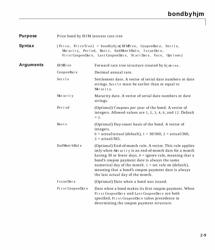
bondbyhjm
2-9
2bondbyhjmPurpose Price bond by HJM interest rate tree
Syntax [Price, PriceTree] = bondbyhjm(HJMTree, CouponRate, Settle,Maturity, Period, Basis, EndMonthRule, IssueDate,FirstCouponDate, LastCouponDate, StartDate, Face, Options)
Arguments HJMTree Forward rate tree structure created by hjmtree.
CouponRate Decimal annual rate.
Settle Settlement date. A vector of serial date numbers or datestrings. Settle must be earlier than or equal toMaturity.
Maturity Maturity date. A vector of serial date numbers or datestrings.
Period (Optional) Coupons per year of the bond. A vector ofintegers. Allowed values are 1, 2, 3, 4, 6, and 12. Default= 2.
Basis (Optional) Day-count basis of the bond. A vector ofintegers.0 = actual/actual (default), 1 = 30/360, 2 = actual/360,3 = actual/365.
EndMonthRule (Optional) End-of-month rule. A vector. This rule appliesonly when Maturity is an end-of-month date for a monthhaving 30 or fewer days. 0 = ignore rule, meaning that abond’s coupon payment date is always the samenumerical day of the month. 1 = set rule on (default),meaning that a bond’s coupon payment date is alwaysthe last actual day of the month.
IssueDate (Optional) Date when a bond was issued.
FirstCouponDate Date when a bond makes its first coupon payment. WhenFirstCouponDate and LastCouponDate are bothspecified, FirstCouponDate takes precedence indetermining the coupon payment structure.

bondbyhjm
2-10
The Settle date for every bond is set to the ValuationDate of the HJM tree.The bond argument Settle is ignored.
Description bondbyhjm is a dynamic programming subroutine for hjmprice.
Price is a number of instruments (NINST)-by-1 matrix of expected prices attime 0.
PriceTree is a structure of trees containing vectors of instrument prices andaccrued interest, and a vector of observation times for each node.
PriceTree.PBush contains the clean prices.
PriceTree.AIBush contains the accrued interest.
PriceTree.tObs contains the observation times.
Examples Price a 4% bond using an HJM forward rate tree.
Load the file deriv.mat, which provides HJMTree. HJMTree contains the timeand forward rate information needed to price the bond.
load deriv
Set the required values. Other arguments will use defaults.
CouponRate = 0.04;Settle = '01-Jan-2000';Maturity = '01-Jan-2004';
LastCouponDate Last coupon date of a bond prior to the maturity date. Inthe absence of a specified FirstCouponDate, a specifiedLastCouponDate determines the coupon structure of thebond. The coupon structure of a bond is truncated at theLastCouponDate regardless of where it falls and will befollowed only by the bond’s maturity cash flow date.
StartDate Ignored.
Face Face value. Default is 100.
Options (Optional) Derivatives pricing options structure createdwith derivset.

bondbyhjm
2-11
Use bondbyhjm to compute the Price of the bond.
Price = bondbyhjm(HJMTree, CouponRate, Settle, Maturity)Warning: Not all cash flows are aligned with the tree. Result willbe approximated.
Price =
107.6773
See Also hjmtree, hjmprice, instbond
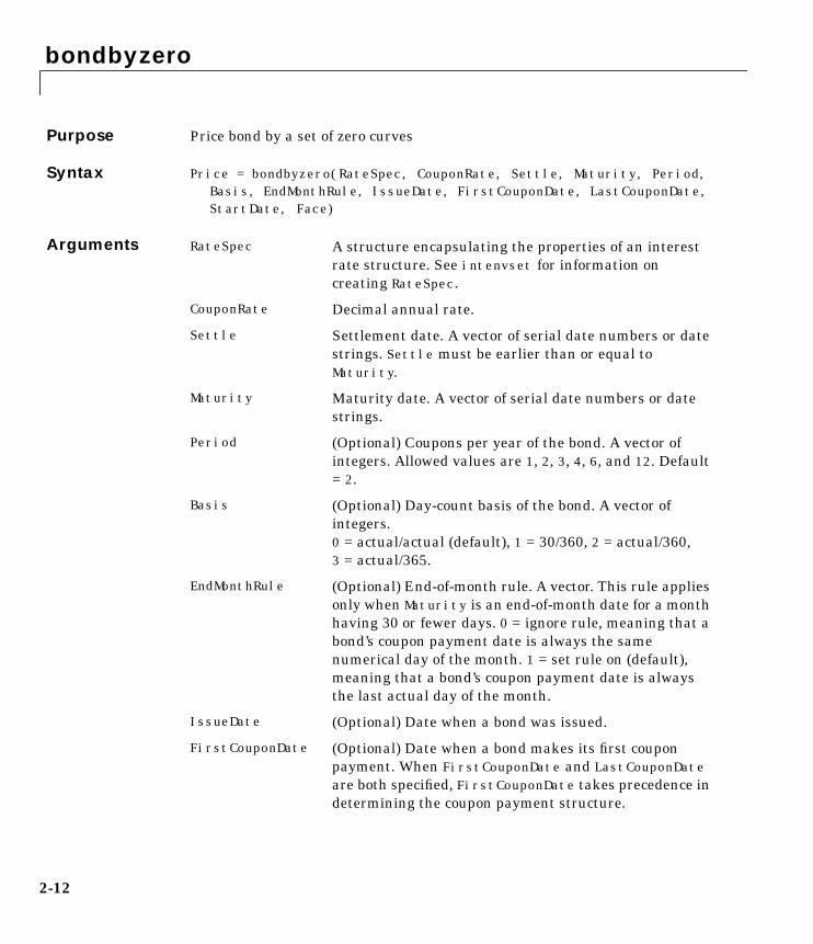
bondbyzero
2-12
2bondbyzeroPurpose Price bond by a set of zero curves
Syntax Price = bondbyzero(RateSpec, CouponRate, Settle, Maturity, Period,Basis, EndMonthRule, IssueDate, FirstCouponDate, LastCouponDate,StartDate, Face)
Arguments RateSpec A structure encapsulating the properties of an interestrate structure. See intenvset for information oncreating RateSpec.
CouponRate Decimal annual rate.
Settle Settlement date. A vector of serial date numbers or datestrings. Settle must be earlier than or equal toMaturity.
Maturity Maturity date. A vector of serial date numbers or datestrings.
Period (Optional) Coupons per year of the bond. A vector ofintegers. Allowed values are 1, 2, 3, 4, 6, and 12. Default= 2.
Basis (Optional) Day-count basis of the bond. A vector ofintegers.0 = actual/actual (default), 1 = 30/360, 2 = actual/360,3 = actual/365.
EndMonthRule (Optional) End-of-month rule. A vector. This rule appliesonly when Maturity is an end-of-month date for a monthhaving 30 or fewer days. 0 = ignore rule, meaning that abond’s coupon payment date is always the samenumerical day of the month. 1 = set rule on (default),meaning that a bond’s coupon payment date is alwaysthe last actual day of the month.
IssueDate (Optional) Date when a bond was issued.
FirstCouponDate (Optional) Date when a bond makes its first couponpayment. When FirstCouponDate and LastCouponDateare both specified, FirstCouponDate takes precedence indetermining the coupon payment structure.

bondbyzero
2-13
All inputs are either scalars or number of instruments (NINST)-by-1 vectorsunless otherwise specified. Dates can be serial date numbers or date strings.Optional arguments can be passed as empty matrix [].
Description Price = bondbyzero(RateSpec, CouponRate, Settle, Maturity, Period,Basis, EndMonthRule, IssueDate, FirstCouponDate, LastCouponDate,StartDate, Face) returns a NINST-by-NUMCURVES matrix of clean bond prices.Each column arises from one of the zero curves.
Examples Price a 4% bond using a set of zero curves.
Load the file deriv.mat, which provides ZeroRateSpec, the interest rate termstructure needed to price the bond.
load deriv
Set the required values. Other arguments will use defaults.
CouponRate = 0.04;Settle = '01-Jan-2000';Maturity = '01-Jan-2004';
Use bondbyzero to compute the Price of the bond.
Price = bondbyzero(ZeroRateSpec, CouponRate, Settle, Maturity)
Price =
107.6912
LastCouponDate (Optional) Last coupon date of a bond prior to thematurity date. In the absence of a specifiedFirstCouponDate, a specified LastCouponDatedetermines the coupon structure of the bond. The couponstructure of a bond is truncated at the LastCouponDateregardless of where it falls and will be followed only bythe bond’s maturity cash flow date.
StartDate Ignored.
Face (Optional) Face value. Default is 100.

bondbyzero
2-14
See Also cfbyzero, fixedbyzero, floatbyzero, swapbyzero
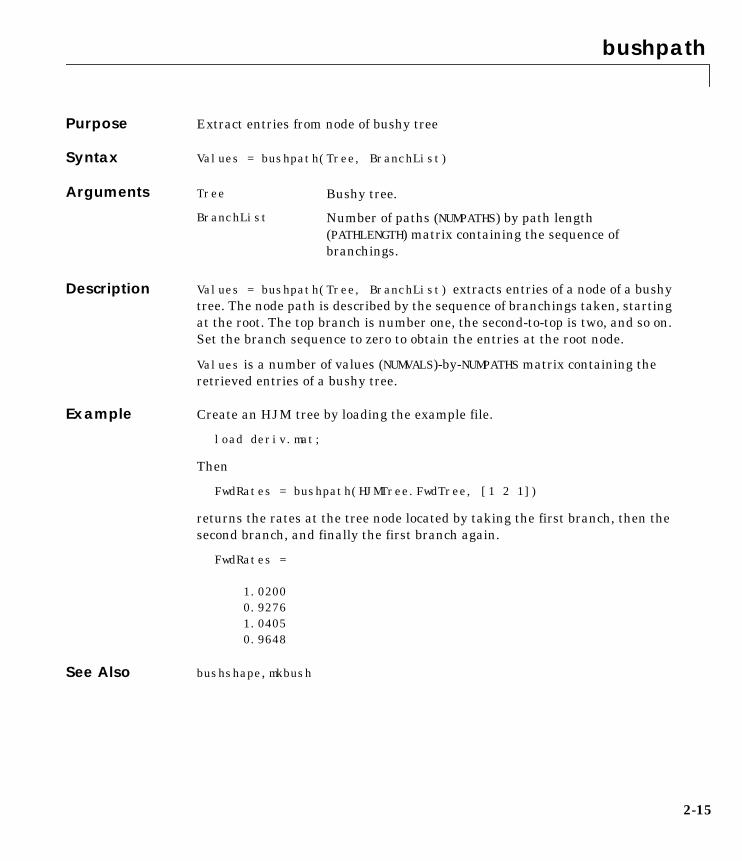
bushpath
2-15
2bushpathPurpose Extract entries from node of bushy tree
Syntax Values = bushpath(Tree, BranchList)
Arguments
Description Values = bushpath(Tree, BranchList) extracts entries of a node of a bushytree. The node path is described by the sequence of branchings taken, startingat the root. The top branch is number one, the second-to-top is two, and so on.Set the branch sequence to zero to obtain the entries at the root node.
Values is a number of values (NUMVALS)-by-NUMPATHS matrix containing theretrieved entries of a bushy tree.
Example Create an HJM tree by loading the example file.
load deriv.mat;
Then
FwdRates = bushpath(HJMTree.FwdTree, [1 2 1])
returns the rates at the tree node located by taking the first branch, then thesecond branch, and finally the first branch again.
FwdRates =
1.0200 0.9276 1.0405 0.9648
See Also bushshape, mkbush
Tree Bushy tree.
BranchList Number of paths (NUMPATHS) by path length(PATHLENGTH) matrix containing the sequence ofbranchings.

bushshape
2-16
2bushshapePurpose Retrieve shape of bushy tree
Syntax [NumLevels, NumChild, NumPos, NumStates, Trim] = bushshape(Tree)
Arguments
Description [NumLevels, NumChild, NumPos, NumStates, Trim] = bushshape(Tree)returns information on a bushy tree’s shape.
NumLevels is the number of time levels of the tree.
NumChild is a 1 by number of levels (NUMLEVELS) vector with the number ofbranches (children) of the nodes in each level.
NumPos is a 1-by-NUMLEVELS vector containing the length of the state vectors ineach level.
NumStates is a 1-by-NUMLEVELS vector containing the number of state vectors ineach level.
Trim is 1 if NumPos decreases by one when moving from one time level to thenext. Otherwise, it is 0.
Example Create an HJM tree by loading the example file.
load deriv.mat;
Then
[NumLevels, NumChild, NumPos, NumStates, Trim]=...bushshape(HJMTree.FwdTree)
returns:
NumLevels = 4
NumChild = 2 2 2 0
NumPos = 4 3 2 1
Tree Bushy tree.

bushshape
2-17
NumStates = 1 2 4 8
Trim = 1
Recreate the tree using the mkbush function:
Tree = mkbush(NumLevels, NumChild(1), NumPos(1), Trim);Tree = mkbush(NumLevels, NumChild, NumPos);
See Also bushpath, mkbush

capbyhjm
2-18
2capbyhjmPurpose Price cap by HJM interest rate tree
Syntax [Price,PriceTree]=capbyhjm(HJMTree, Strike,Settle,Maturity,Reset, Basis, Principal, Options)
Arguments
Description [Price,PriceTree]=capbyhjm(HJMTree,Strike,Settle,Maturity,Reset, Basis, Principal, Options) computes the price of a cap instrumentfrom an HJM tree.
Price is the expected price of the cap at time 0.
PriceTree is the tree structure with values of the cap at each node.
The Settle date for every cap is set to the ValuationDate of the HJM tree. Thecap argument Settle is ignored.
Examples Price a 3% cap instrument using an HJM forward rate tree.
Load the file deriv.mat, which provides HJMTree. HJMTree contains the timeand forward rate information needed to price the cap instrument.
HJMTree Forward rate tree structure created by hjmtree.
Strike Number of instruments (NINST)-by-1 vector of rates atwhich the cap is exercised.
Settle Settlement dates. NINST-by-1 vector of datesrepresenting the settlement dates of the cap.
Maturity NINST-by-1 vector of dates representing the maturitydates of the cap.
Reset (Optional) NINST-by-1 vector representing the resetfrequency per year. Default = 1.
Basis (Optional) NINST-by-1 vector representing the basis usedwhen annualizing the input forward rate tree. Default =0 (actual/actual).
Principal (Optional) The notional principal amount. Default = 100.
Options (Optional) Derivatives pricing options structure createdwith derivset.

capbyhjm
2-19
load deriv
Set the required values. Other arguments will use defaults.
Strike = 0.03;Settle = '01-Jan-2000';Maturity = '01-Jan-2004';
Use capbyhjm to compute the Price of the cap instrument.
Price = capbyhjm(HJMTree, Strike, Settle, Maturity)
Price =
15.4367
See Also cfbyhjm, floorbyhjm, hjmtree, swapbyhjm

cfbyhjm
2-20
2cfbyhjmPurpose Price cash flows from HJM interest rate tree
Syntax [Price, PriceTree] = cfbyhjm(HJMTree, CFlowAmounts, CFlowDates,Settle, Basis, Options)
Arguments
Description [Price, PriceTree] = cfbyhjm(HJMTree, CFlowAmounts, CFlowDates,Settle, Basis, Options) prices cash flows from an HJM interest rate tree.
Price is an NINST-by-1 vector of expected prices at time 0.
PriceTree is a tree structure with a vector of instrument prices at each node.
See Also cfamounts, hjmprice, hjmtree, instcf
HJMTree Forward rate tree structure created by hjmtree.
CFlowAmounts Number of instruments (NINST) by maximum number ofcash flows (MOSTCFS) matrix of cash flow amounts. Eachrow is a list of cash flow values for one instrument. If aninstrument has fewer than MOSTCFS cash flows, the endof the row is padded with NaNs.
CFlowDates NINST-by-MOSTCFSmatrix of cash flow dates. Each entrycontains the date of the corresponding cash flow inCFlowAmounts.
Settle Settlement date. A vector of serial date numbers or datestrings. The Settle date for every cash flow is set to theValuationDate of the HJM tree. The cash flow argument,Settle, is ignored.
Basis (Optional) Day-count basis of the bond. A vector ofintegers.0 = actual/actual (default), 1 = 30/360, 2 = actual/360,3 = actual/365.
Options (Optional) Derivatives pricing options structure createdwith derivset.
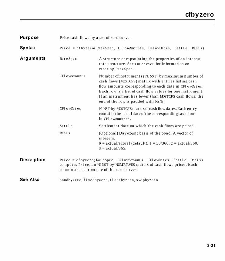
cfbyzero
2-21
2 cfbyzeroPurpose Price cash flows by a set of zero curves
Syntax Price = cfbyzero(RateSpec, CFlowAmounts, CFlowDates, Settle, Basis)
Arguments
Description Price = cfbyzero(RateSpec, CFlowAmounts, CFlowDates, Settle, Basis)computes Price, an NINST-by-NUMCURVES matrix of cash flows prices. Eachcolumn arises from one of the zero curves.
See Also bondbyzero, fixedbyzero, floatbyzero, swapbyzero
RateSpec A structure encapsulating the properties of an interestrate structure. See intenvset for information oncreating RateSpec.
CFlowAmounts Number of instruments (NINST) by maximum number ofcash flows (MOSTCFS) matrix with entries listing cashflow amounts corresponding to each date in CFlowDates.Each row is a list of cash flow values for one instrument.If an instrument has fewer than MOSTCFS cash flows, theend of the row is padded with NaNs.
CFlowDates NINST-by-MOSTCFSmatrixofcashflowdates.Eachentrycontainstheserialdateof thecorrespondingcashflowin CFlowAmounts.
Settle Settlement date on which the cash flows are priced.
Basis (Optional) Day-count basis of the bond. A vector ofintegers.0 = actual/actual (default), 1 = 30/360, 2 = actual/360,3 = actual/365.

classfin
2-22
2classfinPurpose Create financial structure or return financial structure class name
Syntax Obj = classfin(ClassName)Obj = classfin(Struct, ClassName)ClassName = classfin(Obj)
Arguments
Description Obj = classfin(ClassName) and Obj = classfin(Struct, ClassName)create a financial structure of class ClassName.
ClassName = classfin(Obj) returns a string containing a financialstructure’s class name.
Examples Example 1.
Create a HJMTimeSpec financial structure and complete its fields (Typically, thefunction hjmtimespec is used to create HJMTimeSpec structures).
TimeSpec = classfin('HJMTimeSpec');TimeSpec.ValuationDate = datenum('Dec-10-1999');TimeSpec.Maturity = datenum('Dec-10-2000');TimeSpec.Compounding = 2;TimeSpec.Basis = 0;TimeSpec.EndMonthRule = 1;
TimeSpec =
FinObj: 'HJMTimeSpec'
Example 2.
Convert an existing MATLAB structure into a financial structure.
TSpec.ValuationDate = datenum('Dec-10-1999');TSpec.Maturity = datenum('Dec-10-2000');TSpec.Compounding = 2;
ClassName String containing name of financial structure class.
Struct MATLAB structure to be converted into a financialstructure.
Obj Name of a financial structure.

classfin
2-23
TSpec.Basis = 0;TSpec.EndMonthRule = 0;
TimeSpec = classfin(TSpec, 'HJMTimeSpec')
TimeSpec =
ValuationDate: 730464 Maturity: 730830 Compounding: 2 Basis: 0 EndMonthRule: 0 FinObj: 'HJMTimeSpec'
Example 3.
Obtain a financial structure’s class name.
load deriv.matClassName = classfin(HJMTree)
ClassName =
HJMFwdTree
See Also isafin

date2time
2-24
2date2timePurpose Fixed income time and frequency from dates
Syntax [Times, F] = date2time(Settle, Maturity, Compounding, Basis,EndMonthRule)
Arguments Settle Settlement date. A vector of serial date numbers or datestrings. Settle must be earlier than or equal toMaturity.
Maturity Maturity date. A vector of serial date numbers or datestrings.
Compounding Scalar value representing the rate at which the inputzero rates were compounded when annualized. Thisargument determines the formula for the discountfactors:Compounding = 1, 2, 3, 4, 6, 12Disc = (1 + Z/F)^(-T), where F is the compounding
frequency, Z is the zero rate, and T is the time inperiodic units, e.g. T = F is one year.
Compounding = 365Disc = (1 + Z/F)^(-T), where F is the number of days
in the basis year and T is a number of dayselapsed computed by basis.
Compounding = -1Disc = exp(-T*Z), where T is time in years.
Basis (Optional) Day-count basis of the bond. A vector ofintegers.0 = actual/actual (default), 1 = 30/360, 2 = actual/360,3 = actual/365.
EndMonthRule (Optional) End-of-month rule. A vector. This rule appliesonly when Maturity is an end-of-month date for a monthhaving 30 or fewer days. 0 = ignore rule, meaning that abond’s coupon payment date is always the samenumerical day of the month. 1 = set rule on (default),meaning that a bond’s coupon payment date is alwaysthe last actual day of the month.
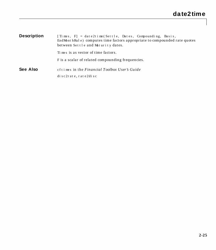
date2time
2-25
Description [Times, F] = date2time(Settle, Dates, Compounding, Basis,EndMonthRule) computes time factors appropriate to compounded rate quotesbetween Settle and Maturity dates.
Times is as vector of time factors.
F is a scalar of related compounding frequencies.
See Also cftimes in the Financial Toolbox User’s Guide
disc2rate, rate2disc

datedisp
2-26
2datedispPurpose Display date entries
Syntax datedisp(NumMat, DateForm)CharMat = datedisp(NumMat, DateForm)
Arguments
Description datedisp(NumMat, DateForm) displays the matrix with the serial datesformatted as date strings, using a matrix with mixed numeric entries andserial date number entries. Integers between datenum('01-Jan-1900') anddatenum('01-Jan-2200') are assumed to be serial date numbers, while allother values are treated as numeric entries.
CharMat is a character array representing NumMat. If no output variable isassigned, the function prints the array to the display.
Example NumMat = [ 730730, 0.03, 1200, 730100; 730731, 0.05, 1000, NaN]
NumMat =
1.0e+05 *
7.3073 0.0000 0.0120 7.3010 7.3073 0.0000 0.0100 NaN
datedisp(NumMat) 01-Sep-2000 0.03 1200 11-Dec-1998 02-Sep-2000 0.05 1000 NaN
See Also datenum, datestr in the Financial Toolbox User’s Guide
Remarks This function is identical to the datedisp function in the Financial Toolbox.
NumMat Numeric matrix to display
DateForm (Optional) Date format. See datestr for available and defaultformat flags.

derivget
2-27
2derivgetPurpose Get derivatives pricing options
Syntax Value = derivget(Options, 'Parameter')
Arguments
Description Value = derivget(Options, 'Parameter') extracts the value of the namedparameter from the derivative options structure Options. Parameter valuescan be 'off' or 'on'.
Examples Create an Options structure with the value of Diagnostics set to 'on'.
Options = derivset('Diagnostics','on')
Use derivget to extract the value of Diagnostics from the Options structure.
Value = derivget(Options, 'Diagnostics')
Value =
on
Use derivget to extract the value of ConstRate.
Value = derivget(Options, 'ConstRate')
Value =
on
Because the value of 'ConstRate' was not previously set with derivset, theanswer represents the default setting for 'ConstRate'.
See Also derivset
Options Existing options specification structure, probablycreated from previous call to derivset.
Parameter Must be 'Diagnostics', 'Warnings', or 'ConstRate'. It issufficient to type only the leading charactersthatuniquelyidentifytheparameter.Caseisignoredforparameter names.

derivset
2-28
2derivsetPurpose Set or modify derivatives pricing options
Syntax Options = derivset(Options, 'Parameter1', Value1, 'Parameter2',Value2,'Parameter3', Value3)
Options = derivset(OldOptions, NewOptions)Options = derivsetderivset
Arguments
Description Options = derivset(Options, 'Parameter1', Value1, 'Parameter2',Value2,'Parameter3', Value3) creates a derivatives pricing optionsstructure Options in which the named parameters have the specified values.Any unspecified value is set to the default value for that parameter whenOptions is passed to the HJM function. It is sufficient to type only the leadingcharacters that uniquely identify the parameter name. Case is also ignored forparameter names.
If the optional input argument Options is specified, derivset modifies anexisting pricing options structure by changing the named parameters to thespecified values.
Options (Optional) Existing options specification structure,probably created from previous call to derivset.
Parametern Must be 'Diagnostics', 'Warnings', or 'ConstRate'.Parameters can be entered in any order. Parametervalues can be 'on' or 'off'.'Diagnostics' 'on' generates diagnostic information.The default is 'Diagnostics' 'off'.'Warnings' 'on' (default) displays a warning messagewhen executing an HJM function.'ConstRate' 'on' (default) assumes a constant ratebetween tree nodes.
OldOptions Existing options specification structure.
NewOptions New options specification structure.

derivset
2-29
Note For parameter values, correct case and the complete string arerequired; if an invalid string is provided, the default is used.
Options = derivset(OldOptions, NewOptions) combines an existingoptions structure OldOptions with a new options structure NewOptions. Anyparameters in NewOptions with nonempty values overwrite the correspondingold parameters in OldOptions.
Options = derivset creates an options structure Options whose fields areset to the default values.
derivset with no input or output arguments displays all parameter namesand information about their possible values.
Examples Options = derivset('Diagnostics','on')
enables the display of additional diagnostic information that appears whenexecuting HJM functions.
Options = derivset(Options, 'ConstRate', 'off')
changes the ConstRate parameter in the existing Options structure so that theassumption of constant rates between tree nodes no longer applies.
With no input or output arguments derivset displays all parameter namesand information about their possible values.
derivset Diagnostics: [ on | {off} ] Warnings: [ {on} | off ] ConstRate: [ {on} | off ]
See Also derivget
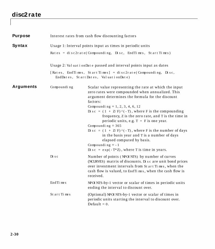
disc2rate
2-30
2disc2ratePurpose Interest rates from cash flow discounting factors
Syntax Usage 1: Interval points input as times in periodic units
Rates = disc2rate(Compounding, Disc, EndTimes, StartTimes)
Usage 2: ValuationDate passed and interval points input as dates
[Rates, EndTimes, StartTimes] = disc2rate(Compounding, Disc,EndDates, StartDates, ValuationDate)
Arguments Compounding Scalar value representing the rate at which the inputzero rates were compounded when annualized. Thisargument determines the formula for the discountfactors:Compounding = 1, 2, 3, 4, 6, 12Disc = (1 + Z/F)^(-T), where F is the compounding
frequency, Z is the zero rate, and T is the time inperiodic units, e.g. T = F is one year.
Compounding = 365Disc = (1 + Z/F)^(-T), where F is the number of days
in the basis year and T is a number of dayselapsed computed by basis.
Compounding = -1Disc = exp(-T*Z), where T is time in years.
Disc Number of points (NPOINTS) by number of curves(NCURVES) matrix of discounts. Disc are unit bond pricesover investment intervals from StartTimes, when thecash flow is valued, to EndTimes, when the cash flow isreceived.
EndTimes NPOINTS-by-1 vector or scalar of times in periodic unitsending the interval to discount over.
StartTimes (Optional) NPOINTS-by-1 vector or scalar of times inperiodic units starting the interval to discount over.Default = 0.

disc2rate
2-31
Description Rates = disc2rate(Compounding, Disc, EndTimes, StartTimes) and
[Rates, EndTimes, StartTimes] = disc2rate(Compounding, Disc,EndDates, StartDates, ValuationDate) convert cash flow discountingfactors to interest rates. disc2rate computes the yields over a series ofNPOINTS time intervals given the cash flow discounts over those intervals.NCURVES different rate curves can be translated at once if they have the sametime structure. The time intervals can represent a zero curve or a forwardcurve.
Rates is an NPOINTS-by-NCURVES column vector of yields in decimal form overthe NPOINTS time intervals.
StartTimes is an NPOINTS-by-1 column vector of times starting the interval todiscount over, measured in periodic units.
EndTimes is an NPOINTS-by-1 column vector of times ending the interval todiscount over, measured in periodic units.
If Compounding = 365 (daily), StartTimes and EndTimes are measured in days.The arguments otherwise contain values, T, computed from SIA semiannualtime factors, Tsemi, by the formula T = Tsemi/2 * F, where F is thecompounding frequency.
The investment intervals can be specified either with input times (Usage 1) orwith input dates (Usage 2). Entering ValuationDate invokes the dateinterpretation; omitting ValuationDate invokes the default timeinterpretations.
See Also rate2disc, ratetimes
EndDates NPOINTS-by-1 vector or scalar of serial maturity datesending the interval to discount over.
StartDates (Optional) NPOINTS-by-1 vector or scalar of serial datesstarting the interval to discount over. Default =ValuationDate.
ValuationDate Scalar value in serial date number form representing theobservation date of the investment horizons entered inStartDates and EndDates. Required in Usage 2. Omittedor passed as an empty matrix to invoke Usage 1.

fixedbyhjm
2-32
2fixedbyhjmPurpose Price fixed rate note from HJM interest rate tree
Syntax [Price, PriceTree] = fixedbyhjm(HJMTree, CouponRate, Settle,Maturity, Reset, Basis, Principal, Options)
Arguments
Description [Price, PriceTree] = fixedbyhjm(HJMTree, CouponRate, Settle,Maturity, Reset, Basis, Principal, Options) is a dynamic programmingsubroutine for hjmprice.
Price is an NINST-by-1 vector of expected prices of the fixed rate note at time 0.
PriceTree is a structure of trees containing vectors of instrument prices andaccrued interest, and a vector of observation times for each node.
PriceTree.PBush contains the clean prices.
PriceTree.AIBush contains the accrued interest.
PriceTree.tObs contains the observation times.
The Settle date for every fixed rate note is set to the ValuationDate of theHJM tree. The fixed rate note argument Settle is ignored.
HJMTree Forward rate tree structure created by hjmtree.
CouponRate Decimal annual rate.
Settle Settlement dates. Number of instruments (NINST)-by-1vector of dates representing the settlement dates of thefixed rate note.
Maturity NINST-by-1 vector of dates representing the maturitydates of the fixed rate note.
Reset NINST-by-1 vector representing the reset frequency peryear. Default = 1.
Basis NINST-by-1 vector representing the basis used whenannualizing the input forward rate tree. Default = 0(actual/actual).
Principal The notional principal amount. Default = 100.
Options (Optional) Derivatives pricing options structure createdwith derivset.

fixedbyhjm
2-33
Examples Price a 4% fixed rate note using an HJM forward rate tree.
Load the file deriv.mat, which provides HJMTree. HJMTree contains the timeand forward rate information needed to price the note.
load deriv
Set the required values. Other arguments will use defaults.
CouponRate = 0.04;Settle = '01-Jan-2000';Maturity = '01-Jan-2003';
Use fixedbyhjm to compute the Price of the note.
Price = fixedbyhjm(HJMTree, CouponRate, Settle, Maturity, Reset)
Price =
105.7678
See Also bondbyhjm, capbyhjm, cfbyhjm, floatbyhjm, floorbyhjm, hjmtree, swapbyhjm

fixedbyzero
2-34
2fixedbyzeroPurpose Price fixed rate note by a set of zero curves
Syntax Price = fixedbyzero(RateSpec, CouponRate, Settle, Maturity, Reset,Basis, Principal)
Arguments
All inputs are either scalars or NINST-by-1 vectors unless otherwisespecified. Any date may be a serial date number or date string. An optionalargument may be passed as an empty matrix [].
Description Price = fixedbyzero(RateSpec, CouponRate, Settle, Maturity, Reset,Basis, Principal) computes the price of a fixed rate note by a set of zerocurves.
Price is a number of instruments (NINST) by number of curves (NUMCURVES)matrix of fixed rate note prices. Each column arises from one of the zero curves.
Examples Price a 4% fixed rate note using a set of zero curves.
Load the file deriv.mat, which provides ZeroRateSpec, the interest rate termstructure needed to price the note.
load deriv
Set the required values. Other arguments will use defaults.
RateSpec A structure encapsulating the properties of an interestrate structure. See intenvset for information oncreating RateSpec.
CouponRate Decimal annual rate.
Settle Settlement date. Settle must be earlier than or equal toMaturity.
Maturity Maturity date.
Reset (Optional) Frequency of settlements per year. Default =1.
Basis (Optional) Day count basis. Default = 0 (actual/actual).
Principal (Optional) The notional principal amount. Default = 100.

fixedbyzero
2-35
CouponRate = 0.04;Settle = '01-Jan-2000';Maturity = '01-Jan-2003';
Use fixedbyzero to compute the Price of the note.
Price = fixedbyzero(ZeroRateSpec, CouponRate, Settle, Maturity)
Price =
105.7678
See Also bondbyzero, cfbyzero, floatbyzero, swapbyzero
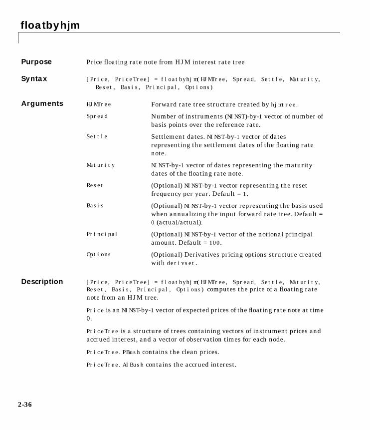
floatbyhjm
2-36
2floatbyhjmPurpose Price floating rate note from HJM interest rate tree
Syntax [Price, PriceTree] = floatbyhjm(HJMTree, Spread, Settle, Maturity,Reset, Basis, Principal, Options)
Arguments
Description [Price, PriceTree] = floatbyhjm(HJMTree, Spread, Settle, Maturity,Reset, Basis, Principal, Options) computes the price of a floating ratenote from an HJM tree.
Price is an NINST-by-1 vector of expected prices of the floating rate note at time0.
PriceTree is a structure of trees containing vectors of instrument prices andaccrued interest, and a vector of observation times for each node.
PriceTree.PBush contains the clean prices.
PriceTree.AIBush contains the accrued interest.
HJMTree Forward rate tree structure created by hjmtree.
Spread Number of instruments (NINST)-by-1 vector of number ofbasis points over the reference rate.
Settle Settlement dates. NINST-by-1 vector of datesrepresenting the settlement dates of the floating ratenote.
Maturity NINST-by-1 vector of dates representing the maturitydates of the floating rate note.
Reset (Optional) NINST-by-1 vector representing the resetfrequency per year. Default = 1.
Basis (Optional) NINST-by-1 vector representing the basis usedwhen annualizing the input forward rate tree. Default =0 (actual/actual).
Principal (Optional) NINST-by-1 vector of the notional principalamount. Default = 100.
Options (Optional) Derivatives pricing options structure createdwith derivset.

floatbyhjm
2-37
PriceTree.tObs contains the observation times.
The Settle date for every floating rate note is set to the ValuationDate of theHJM tree. The floating rate note argument Settle is ignored.
Examples Price a 20 basis point floating rate note using an HJM forward rate tree.
Load the file deriv.mat, which provides HJMTree. HJMTree contains the timeand forward rate information needed to price the note.
load deriv
Set the required values. Other arguments will use defaults.
Spread = 20;Settle = '01-Jan-2000';Maturity = '01-Jan-2003';
Use floatbyhjm to compute the Price of the note.
Price = floatbyhjm(HJMTree, Spread, Settle, Maturity)
Price =
100.5768
See Also bondbyhjm, capbyhjm, cfbyhjm, fixedbyhjm, floorbyhjm, hjmtree, swapbyhjm

floatbyzero
2-38
2floatbyzeroPurpose Price floating rate note prices by a set of zero curves
See Also Price = floatbyzero(RateSpec, Spread, Settle, Maturity, Reset,Basis, Principal)
Arguments
All inputs are either scalars or NINST-by-1 vectors unless otherwisespecified. Any date may be a serial date number or date string. An optionalargument may be passed as an empty matrix [].
Description Price = floatbyzero(RateSpec, Spread, Settle, Maturity, Reset,Basis, Principal) computes the price of a floating rate note by a set of zerocurves.
Price is a number of instruments (NINST) by number of curves (NUMCURVES)matrix of floating rate note prices. Each column arises from one of the zerocurves.
Examples Price a 20 basis point floating rate note using a set of zero curves.
Load the file deriv.mat, which provides ZeroRateSpec, the interest rate termstructure needed to price the note.
load deriv
Set the required values. Other arguments will use defaults.
RateSpec A structure encapsulating the properties of an interestrate structure. See intenvset for information oncreating RateSpec.
Spread Number of basis points over the reference rate.
Settle Settlement date. Settle must be earlier than or equal toMaturity.
Maturity Maturity date.
Reset (Optional) Frequency of settlements per year. Default =1.
Basis (Optional) Day count basis. Default = 0 (actual/actual).
Principal (Optional) The notional principal amount. Default = 100.
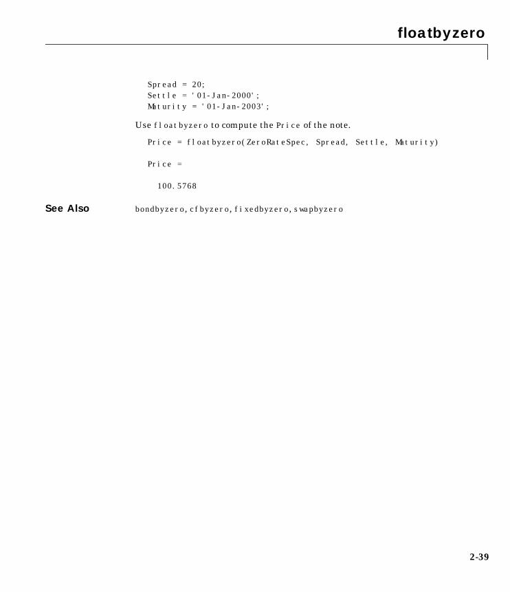
floatbyzero
2-39
Spread = 20;Settle = '01-Jan-2000';Maturity = '01-Jan-2003';
Use floatbyzero to compute the Price of the note.
Price = floatbyzero(ZeroRateSpec, Spread, Settle, Maturity)
Price =
100.5768
See Also bondbyzero, cfbyzero, fixedbyzero, swapbyzero

floorbyhjm
2-40
2floorbyhjmPurpose Price floor by HJM interest rate tree
Syntax [Price, PriceTree] = floorbyhjm(HJMTree, Strike, Settle, Maturity,Reset, Basis, Principal, Options)
Arguments
Description [Price, PriceTree] = floorbyhjm(HJMTree, Strike, Settlement,Maturity, Reset, Basis, Principal, Options) computes the price of afloor instrument from an HJM tree.
Price is an NINST-by-1 vector of the expected prices of the floor at time 0.
PriceTree is the tree structure with values of the floor at each node.
Examples Price a 1% floor instrument using an HJM forward rate tree.
Load the file deriv.mat, which provides HJMTree. HJMTree contains the timeand forward rate information needed to price the floor instrument.
HJMTree Forward rate tree structure created by hjmtree.
Strike Number of instruments (NINST)-by-1 vector of rates atwhich the floor is exercised.
Settle Settlement date. NINST-by-1 vector of dates representingthe settlement dates of the floor. The Settle date forevery floor is set to the ValuationDate of the HJM tree.The floor argument Settle is ignored.
Maturity NINST-by-1 vector of dates representing the maturitydates of the floor.
Reset (Optional) NINST-by-1 vector representing the resetfrequency per year. Default = 1.
Basis (Optional) NINST-by-1 vector representing the basis usedwhen annualizing the input forward rate tree. Default =0 (actual/actual).
Principal (Optional) The notional principal amount. Default = 100.
Options (Optional) Derivatives pricing options structure createdwith derivset.

floorbyhjm
2-41
load deriv
Set the required values. Other arguments will use defaults.
Strike = 0.01;Settle = '01-Jan-2000';Maturity = '01-Jan-2004';
Use floorbyhjm to compute the Price of the floor instrument.
Price = floorbyhjm(HJMTree, Strike, Settle, Maturity)
Price =
15.3938
See Also capbyhjm, cfbyhjm, hjmtree, swapbyhjm

hedgeopt
2-42
2hedgeoptPurpose Allocate optimal hedge for target costs or sensitivities
Syntax [PortSens, PortCost, PortHolds] = hedgeopt(Sensitivities, Price,CurrentHolds, FixedInd, NumCosts, TargetCost, TargetSens,ConSet)
Arguments Sensitivities Number of instruments (NINST) by number ofsensitivities (NSENS) matrix of dollar sensitivities of eachinstrument. Each row represents a different instrument.Each column represents a different sensitivity.
Price NINST-by-1 vector of portfolio instrument unit prices.
CurrentHolds NINST-by-1 vector of contracts allocated to eachinstrument.
FixedInd (Optional) Number of fixed instruments (NFIXED)-by-1vector of indices of instruments to hold fixed. Forexample, to hold the first and third instruments of a 10instrument portfolio unchanged, set FixedInd = [1 3].Default = [], no instruments held fixed.
NumCosts (Optional) Number of points generated along the costfrontier when a vector of target costs (TargetCost) is notspecified. The default is 10 equally-spaced pointsbetween the point of minimum cost and the point ofminimum exposure. When specifying TargetCost, enterNumCosts as an empty matrix [].
TargetCost (Optional) Vector of target cost values along the costfrontier. If TargetCost is empty, or not entered,hedgeopt evaluates NumCosts equally-spaced targetcosts between the minimum cost and minimumexposure. When specified, the elements of TargetCostshould be positive numbers that represent the maximumamount of money the owner is willing to spend torebalance the portfolio.

hedgeopt
2-43
Notes 1. The user-specified constraints included in ConSet may be createdwith the functions pcalims or portcons. However, the portcons defaultPortHolds positivity constraints are typically inappropriate for hedgingproblems since short-selling is usually required.
2. NPOINTS, the number of rows in PortSens and PortHolds and the length ofPortCost, is inferred from the inputs. When the target sensitivities,TargetSens, is entered, NPOINTS = 1; otherwise NPOINTS = NumCosts, or isequal to the length of the TargetCost vector.
3. Not all problems are solvable (e.g., the solution space may be infeasibleor unbounded, or the solution may fail to converge). When a valid solutionis not found, the corresponding rows of PortSens and PortHolds and theelements of PortCost are padded with NaN’s as placeholders.
Description [PortSens, PortCost, PortHolds] = hedgeopt(Sensitivities, Price,CurrentHolds, FixedInd, NumCosts, TargetCost, TargetSens, ConSet)allocates an optimal hedge by one of two criteria:
1 Minimize portfolio sensitivities (exposure) for a given set of target costs
2 Minimize the cost of hedging a portfolio given a set of target sensitivities.
Hedging involves the fundamental tradeoff between portfolio insurance andthe cost of insurance coverage. This function allows investors to modify
TargetSens (Optional) 1-by-NSENS vector containing the targetsensitivity values of the portfolio. When specifyingTargetSens, enter NumCosts and TargetCost as emptymatrices [].
ConSet (Optional) Number of constraints (NCONS) by number ofinstruments (NINST) matrix of additional conditions onthe portfolio reallocations. An eligible NINST-by-1 vectorof contract holdings, PortWts, satisfies all theinequalities A*PortWts <= b, whereA = ConSet(:,1:end-1) and b = ConSet(:,end).

hedgeopt
2-44
portfolio allocations among instruments to achieve either of the criteria. Thechosen criterion is inferred from the input argument list. The problem is castas a constrained linear least-squares problem.
PortSens is a number of points (NPOINTS)-by-NSENS matrix of portfoliosensitivities. When a perfect hedge exists, PortSens is zeros. Otherwise, thebest hedge possible is chosen.
PortCost is a 1-by-NPOINTS vector of total portfolio costs.
PortHolds is an NPOINTS-by-NINST matrix of contracts allocated to eachinstrument. These are the reallocated portfolios.
See Also hedgeslf
pcalims, portcons, portopt in the Financial Toolbox User’s Guide
lsqlin in the Optimization Toolbox User’s Guide

hedgeslf
2-45
2hedgeslfPurpose Self-financing hedge
Syntax [PortSens, PortValue, PortHolds] = hedgeslf(Sensitivities, Price,CurrentHolds, FixedInd, ConSet)
Arguments
Description [PortSens, PortValue, PortHolds] = hedgeslf(Sensitivities, Price,CurrentHolds, FixedInd, ConSet) allocates a self-financing hedge among acollection of instruments. hedgeslf finds the reallocation in a portfolio offinancial instruments that hedges the portfolio against market moves and thatis closest to being self-financing (maintaining constant portfolio value). Bydefault the first instrument entered is hedged with the other instruments.
PortSens is a 1-by-NSENS vector of portfolio dollar sensitivities. When a perfecthedge exists, PortSens is zeros. Otherwise the best hedge possible is chosen.
Sensitivities Number of instruments (NINST) by number ofsensitivities (NSENS) matrix of dollar sensitivities of eachinstrument. Each row represents a different instrument.Each column represents a different sensitivity.
Price NINST-by-1 vector of instrument unit prices.
CurrentHolds NINST-by-1 vector of contracts allocated in eachinstrument.
FixedInd (Optional) Empty or number of fixed instruments(NFIXED)-by-1 vector of indices of instruments to holdfixed. The default is FixedInd = 1; the holdings in thefirst instrument will be held fixed. If NFIXED instrumentswill not be changed, enter all their locations in theportfolio in a vector. If no instruments are to be heldfixed, enter FixedInd = [].
ConSet (Optional) Number of constraints (NCONS)-by-NINSTmatrix of additional conditions on the portfolioreallocations. An eligible NINST-by-1 vector of contractholdings, PortHolds, satisfies all the inequalities
A*PortHolds <= b, whereA = ConSet(:,1:end-1) and b = ConSet(:,end).

hedgeslf
2-46
PortValue is the total portfolio value (scalar). When a perfectly self-financinghedge exists, PortValue is equal to the value, dot(Price, CurrentWts), of theinitial portfolio.
PortHolds is an NINST-by-1 vector of contracts allocated to each instrument.This is the reallocated portfolio.
Notes 1. The constraints PortHolds(FixedInd) = CurrentHolds(FixedInd)are appended to any constraints passed in ConSet. Pass FixedInd = [] tospecify all constraints through ConSet.
2. The default constraints generated by portcons are inappropriate, sincethey require the sum of all holdings to be positive and equal to one.
3. hedgeself first tries to find the allocations of the portfolio that make itclosest to being self-financing, while reducing the sensitivities to 0. If nosolution is found, it finds the allocations that minimize the sensitivities. If theresulting portfolio is self-financing, PortValue is equal to the value of theoriginal portfolio.
Examples Example 1. Perfect Sensitivity Unreachable.
Sens = [0.44 0.32; 1.0 0.0]Price = [1.2; 1.0]W0 = [1; 1][PortSens, PortValue, PortHolds]= hedgeslf(Sens, Price, W0)
PortSens =
0.0000 0.3200
PortValue =
0.7600

hedgeslf
2-47
PortHolds =
1.0000 -0.4400
Example 2. Conflicting Constraints.
Sens = [0.44 0.32; 1.0 0.0]Price = [1.2; 1.0]W0 = [1; 1]ConSet = pcalims([2 2])
% O.K. if nothing fixed.
[PortSens, PortValue, PortHolds]= hedgeslf(Sens, Price, W0,...[], ConSet)
PortSens =
2.8800 0.6400
PortValue =
4.4000
PortHolds =
2 2
% W0(1) is not greater than 2.
[PortSens, PortValue, PortHolds] = hedgeslf(Sens, Price, W0,...1, ConSet)
??? Error using ==> hedgeslfOverly restrictive allocation constraints implied by ConSet andby fixing the weight of instruments(s): 1
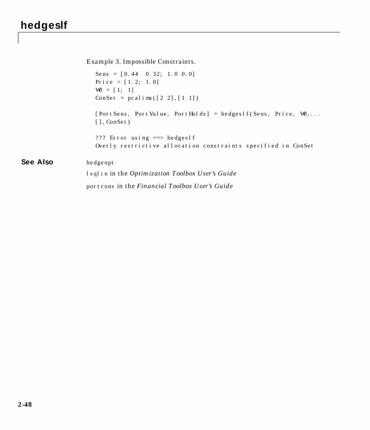
hedgeslf
2-48
Example 3. Impossible Constraints.
Sens = [0.44 0.32; 1.0 0.0]Price = [1.2; 1.0]W0 = [1; 1]ConSet = pcalims([2 2],[1 1])
[PortSens, PortValue, PortHolds] = hedgeslf(Sens, Price, W0,...[],ConSet)
??? Error using ==> hedgeslfOverly restrictive allocation constraints specified in ConSet
See Also hedgeopt
lsqlin in the Optimization Toolbox User’s Guide
portcons in the Financial Toolbox User’s Guide

hjmprice
2-49
2 hjmpricePurpose Fixed income instrument prices by HJM interest rate tree
Syntax [Price, PriceTree] = hjmprice(HJMTree, InstSet, Options)
Arguments
Description Price = hjmprice(HJMTree, InstSet, Options) computes arbitrage freeprices for instruments using an interest rate tree created with hjmtree. NINSTinstruments from a financial instrument variable, InstSet, are priced.
Price is a NINST-by-1 vector of prices for each instrument. The prices arecomputed by backward dynamic programming on the interest rate tree. If aninstrument cannot be priced, NaN is returned.
PriceTree is a structure containing a bushy tree with NINST-by-1 price vectorsat every state.
hjmprice handles instrument types: 'Bond', 'CashFlow', 'OptBond', 'Fixed','Float', 'Cap', 'Floor', 'Swap'. See instadd to construct defined types.
See single-type pricing functions to retrieve state by state pricing treeinformation.
• bondbyhjm: Price a bond by an HJM tree.
• capbyhjm: Price a cap by an HJM tree.
• cfbyhjm: Price an arbitrary set of cash flows by an HJM tree.
• fixedbyhjm: Price a fixed rate note by an HJM tree.
• floatbyhjm: Price a floating rate note by an HJM tree.
• floorbyhjm: Price a floor by an HJM tree.
HJMTree Heath-Jarrow-Morton tree sampling a forward rateprocess. See hjmtree for information on creatingHJMTree.
InstSet Variable containing a collection of instruments.Instruments are categorized by type; each type can havedifferent data fields. The stored data field is a row vectoror string for each instrument.
Options (Optional) Derivatives pricing options structure createdwith derivset.

hjmprice
2-50
• optbndbyhjm: Price a bond option by an HJM tree.
• swapbyhjm: Price a swap by an HJM tree.
Example Load the tree and instruments from a data file. Price the cap and bondinstruments contained in the instrument set.
load deriv.mat;HJMSubSet = instselect(HJMInstSet,'Type', {'Bond', 'Cap'});
instdisp(HJMSubSet)
Index Type CouponRate Settle Maturity Period Name ...1 Bond 0.04 01-Jan-2000 01-Jan-2003 1 4% bond2 Bond 0.04 01-Jan-2000 01-Jan-2004 2 4% bond
Index Type Strike Settle Maturity CapReset... Name ...3 Cap 0.03 01-Jan-2000 01-Jan-2004 1 3% Cap
Price = hjmprice(HJMTree, HJMSubSet)
Warning: Not all cash flows are aligned with the tree. Result willbe approximated.
Price =
105.7678 107.6773 15.4367
See Also hjmsens, hjmtree, hjmvolspec, instadd, intenvprice, intenvsens

hjmsens
2-51
2hjmsensPurpose Fixed income instrument prices and sensitivities by HJM interest rate tree
Syntax [Delta, Gamma, Vega, Price] = hjmsens(HJMTree, InstSet, Options)
Arguments
Description [Delta, Gamma, Vega, Price] = hjmsens(HJMTree, InstSet, Options)computes instrument sensitivities and prices for instruments using an interestrate tree created with hjmtree. NINST instruments from a financial instrumentvariable, InstSet, are priced. hjmsens handles instrument types: 'Bond','CashFlow', 'OptBond', 'Fixed', 'Float', 'Cap', 'Floor', 'Swap'. Seeinstadd for information on instrument types.
Delta is an NINST-by-1 vector of deltas, representing the rate of change ofinstrument prices with respect to changes in the interest rate. Delta iscomputed by finite differences in calls to hjmtree. See hjmtree for informationon the observed yield curve.
Gamma is an NINST-by-1 vector of gammas, representing the rate of change ofinstrument deltas with respect to the changes in the interest rate. Gamma iscomputed by finite differences in calls to hjmtree.
Vega is an NINST-by-1 vector of vegas, representing the rate of change ofinstrument prices with respect to the changes in the volatility, Sigma(t,T).Vega is computed by finite differences in calls to hjmtree. See hjmvolspec forinformation on the volatility process.
HJMTree Heath-Jarrow-Morton tree sampling a forward rateprocess. See hjmtree for information on creatingHJMTree.
InstSet Variable containing a collection of instruments.Instruments are categorized by type; each type can havedifferent data fields. The stored data field is a row vectoror string for each instrument.
Options (Optional) Derivatives pricing options structure createdwith derivset.
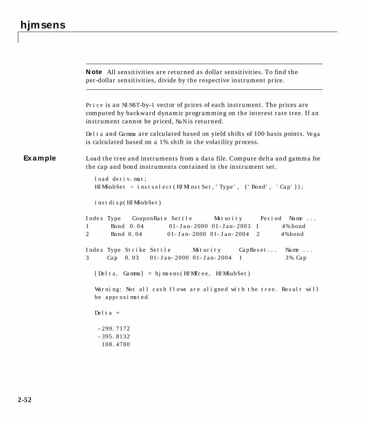
hjmsens
2-52
Note All sensitivities are returned as dollar sensitivities. To find theper-dollar sensitivities, divide by the respective instrument price.
Price is an NINST-by-1 vector of prices of each instrument. The prices arecomputed by backward dynamic programming on the interest rate tree. If aninstrument cannot be priced, NaN is returned.
Delta and Gamma are calculated based on yield shifts of 100 basis points. Vegais calculated based on a 1% shift in the volatility process.
Example Load the tree and instruments from a data file. Compute delta and gamma forthe cap and bond instruments contained in the instrument set.
load deriv.mat;HJMSubSet = instselect(HJMInstSet,'Type', {'Bond', 'Cap'});
instdisp(HJMSubSet)
Index Type CouponRate Settle Maturity Period Name ...1 Bond 0.04 01-Jan-2000 01-Jan-2003 1 4% bond2 Bond 0.04 01-Jan-2000 01-Jan-2004 2 4% bond
Index Type Strike Settle Maturity CapReset... Name ...3 Cap 0.03 01-Jan-2000 01-Jan-2004 1 3% Cap
[Delta, Gamma] = hjmsens(HJMTree, HJMSubSet)
Warning: Not all cash flows are aligned with the tree. Result willbe approximated.
Delta =
-299.7172 -395.8132 108.4780

hjmsens
2-53
Gamma =
1.0e+003 *
1.1603 1.9012 -0.6975
See Also hjmprice, hjmtree, hjmvolspec, instadd

hjmtimespec
2-54
2hjmtimespecPurpose Specify time structure for HJM interest rate tree
Syntax TimeSpec = hjmtimespec(ValuationDate, Maturity, Compounding)
Arguments
Description TimeSpec = hjmtimespec(ValuationDate, Maturity, Compounding) setsthe number of levels and node times for an HJM tree and determines themapping between dates and time for rate quoting.
TimeSpec is a structure specifying the time layout for hjmtree. The stateobservation dates are [Settle; Maturity(1:end-1)]. Because a forward rateis stored at the last observation, the tree can value cash flows out to Maturity.
Example Specify an eight period tree with semiannual nodes (every six months). Useexponential compounding to report rates.
ValuationDate Scalar date marking the pricing date and firstobservation in the tree. Specify as serial date number ordate string
Maturity Number of levels (depth) of the tree. A number of levels(NLEVELS)-by-1 vector of dates marking the cash flowdates of the tree. Cash flows with these maturities fall ontree nodes. Maturity should be in increasing order.
Compounding (Optional) Scalar value representing the rate at whichthe input zero rates were compounded when annualized.Default = 1. This argument determines the formula forthe discount factors:Compounding = 1, 2, 3, 4, 6, 12Disc = (1 + Z/F)^(-T), where F is the compounding
frequency, Z is the zero rate, and T is the time inperiodic units, e.g. T = F is one year.
Compounding = 365Disc = (1 + Z/F)^(-T), where F is the number of days
in the basis year and T is a number of dayselapsed computed by basis.
Compounding = -1Disc = exp(-T*Z), where T is time in years.

hjmtimespec
2-55
Compounding = -1ValuationDate = '15-Jan-1999'Maturity = datemnth(ValuationDate, 6*(1:8)')TimeSpec = hjmtimespec(ValuationDate, Maturity, Compounding)
TimeSpec =
FinObj: 'HJMTimeSpec' ValuationDate: 730135 Maturity: [8x1 double] Compounding: -1 Basis: 0 EndMonthRule: 1
See Also hjmtree, hjmvolspec

hjmtree
2-56
2hjmtreePurpose Build an HJM forward rate tree
Syntax HJMTree = hjmtree(VolSpec, RateSpec, TimeSpec)
Arguments
Description HJMTree = hjmtree(VolSpec, RateSpec, TimeSpec) creates a structurecontaining time and forward rate information on a bushy tree.
See Also hjmprice, hjmtimespec, hjmvolspec, intenvset
VolSpec Volatility process specification. Sets the number offactors and the rules for computing the volatilitysigma(t,T) for each factor. See hjmvolspec forinformation on the volatility process.
RateSpec Interest rate specification for the initial rate curve. Seeintenvset for information on declaring an interest ratevariable.
TimeSpec Tree time layout specification. Defines the observationdates of the HJM tree and the Compounding rule for dateto time mapping and price-yield formulas. Seehjmtimespec for information on the tree structure.
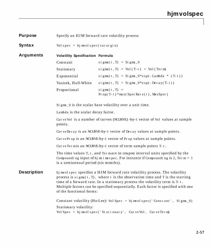
hjmvolspec
2-57
2hjmvolspecPurpose Specify an HJM forward rate volatility process
Syntax Volspec = hjmvolspec(varargin)
Arguments
Sigma_0 is the scalar base volatility over a unit time.
Lambda is the scalar decay factor.
CurveVol is a number of curves (NCURVE) -by-1 vector of Vol values at samplepoints.
CurveDecay is an NCURVE-by-1 vector of Decay values at sample points.
CurveProp is an NCURVE-by-1 vector of Prop values at sample points.
CurveTerm is an NCURVE-by-1 vector of term sample points T-t.
The time values T, t, and Term are in coupon interval units specified by theCompounding input of hjmtimespec. For instance if Compounding is 2, Term = 1is a semiannual period (six months).
Description hjmvolspec specifies a HJM forward rate volatility process. The volatilityprocess is sigma(t,T), where t is the observation time and T is the startingtime of a forward rate. In a stationary process the volatility term is T-t.Multiple factors can be specified sequentially. Each factor is specified with oneof the functional forms:
Constant volatility (Ho-Lee): VolSpec = hjmvolspec('Constant', Sigma_0)
Stationary volatility:VolSpec = hjmvolspec('Stationary', CurveVol, CurveTerm)
Volatility Specification Formula
Constant sigma(t,T) = Sigma_0
Stationary sigma(t,T) = Vol(T-t) = Vol(Term)
Exponential sigma(t,T) = Sigma_0*exp(-Lambda * (T-t))
Vasicek, Hull-White sigma(t,T) = Sigma_0*exp(-Decay(T-t))
Proportional sigma(t,T) =Prop(T-t)*max(SpotRate(t),MaxSpot)

hjmvolspec
2-58
Exponential volatility:VolSpec = hjmvolspec('Exponential', Sigma_0, Lambda)
Vasicek, Hull-White:VolSpec = hjmvolspec('Vasicek', Sigma_0, CurveDecay, CurveTerm)
Nearly proportional stationary:VolSpec = hjmvolspec('Proportional', CurveProp, CurveTerm, MaxSpot)
VolSpec is a structure specifying the volatility model for hjmtree.
Example Single-factor proportional
CurveProp = [0.11765; 0.08825; 0.06865];CurveTerm = [1; 2; 3];VolSpec = hjmvolspec('Proportional', CurveProp, CurveTerm, 1e6)
VolSpec = FinObj: 'HJMVolSpec' FactorModels: {'Proportional'} FactorArgs: {{1x3 cell}} SigmaShift: 0 NumFactors: 1 NumBranch: 2 PBranch: [0.5000 0.5000] Fact2Branch: [-1 1]
Two-factor exponential and constant
VolSpec = hjmvolspec('Exponential', 0.1, 1, 'Constant', 0.2)
VolSpec = FinObj: 'HJMVolSpec' FactorModels: {'Exponential' 'Constant'} FactorArgs: {{1x2 cell} {1x1 cell}} SigmaShift: 0 NumFactors: 2 NumBranch: 3 PBranch: [0.2500 0.2500 0.5000] Fact2Branch: [2x3 double]
See Also hjmtimespec, hjmtree

instadd
2-59
2instaddPurpose Add types to instrument collection
Syntax Bond instrument. (See also instbond.)InstSet = instadd('Bond', CouponRate, Settle, Maturity, Period,
Basis, EndMonthRule, IssueDate, FirstCouponDate, LastCouponDate,StartDate, Face)
Arbitrary cash flow instrument. (See also instcf.)InstSet = instadd('CashFlow', CFlowAmounts, CFlowDates, Settle,
Basis)
Bond option. (See also instoptbnd.)InstSet = instadd('OptBond', BondIndex, OptSpec, Strike,
ExerciseDates, AmericanOpt)
Fixed rate note instrument. (See also instfixed.)InstSet = instadd('Fixed', CouponRate, Settle, Maturity, Reset,
Basis, Principal) )
Floating rate note instrument. (See also instfloat.)InstSet = instadd('Float', Spread, Settle, Maturity, Reset, Basis,
Principal )
Cap instrument. (See also instcap.)InstSet = instadd('Cap', Strike, Settle, Maturity, Reset, Basis,
Principal)
Floor instrument. (See also instfloor.)InstSet = instadd('Floor', Strike, Settle, Maturity, Reset, Basis,
Principal)
Swap instrument. (See also instswap.)InstSet = instadd('Swap', LegRate, Settle, Maturity, LegReset,
Basis, Principal, LegType)
To add instruments to an existing collection:InstSet = instadd(InstSetOld, TypeString, Data1, Data2, ...)

instadd
2-60
Arguments For more information on instrument data parameters, see the reference entriesfor individual instrument types. For example, see instcap for additionalinformation on the cap instrument.
Description instadd stores instruments of types 'Bond', 'CashFlow', 'OptBond', 'Fixed','Float', 'Cap', 'Floor', or 'Swap'. Pricing and sensitivity routines areprovided for these instruments.
InstSet is an instrument set variable containing the new input data.
Example Create a portfolio with two cap instruments and a 4% bond.
Strike = [0.06; 0.07];CouponRate = 0.04;Settle = '06-Feb-2000';Maturity = '15-Jan-2003';
InstSet = instadd('Cap', Strike, Settle, Maturity);InstSet = instadd(InstSet, 'Bond', CouponRate, Settle, Maturity);instdisp(InstSet)
Index Type Strike Settle Maturity CapReset Basis Principal1 Cap 0.06 06-Feb-2000 15-Jan-2003 NaN NaN NaN2 Cap 0.07 06-Feb-2000 15-Jan-2003 NaN NaN NaN
Index Type CouponRate Settle Maturity ...3 Bond 0.04 06-Feb-2000 15-Jan-2003...
See Also instbond, instcap, instcf, instfixed, instfloat, instfloor, instoptbnd,instswap
InstSetOld Variable containing a collection of instruments.Instruments are classified by type; each type can havedifferent data fields. The stored data field is a row vectoror string for each instrument.

instaddfield
2-61
2instaddfieldPurpose Add new instruments to an instrument collection
Syntax InstSet = instaddfield('FieldName', FieldList,'Data', DataList,'Type',TypeString)
InstSet = instaddfield('FieldName', FieldList, 'FieldClass',ClassList, 'Data', DataList, 'Type',TypeString)
InstSetNew = instaddfield(InstSet,'FieldName', FieldList, 'Data',DataList, 'Type',TypeString)
Arguments FieldList String or number of fields (NFIELDS)-by-1 cell array ofstrings listing the name of each data field. FieldListcannot be named with the reserved names Type orIndex.
DataList Number of instruments (NINST)-by-M array orNFIELDS-by-1 cell array of data contents for each field.Each row in a data array corresponds to a separateinstrument. Single rows are copied to apply to allinstruments to be worked on. The number of columns isarbitrary, and data will be padded along columns.
ClassList (Optional) String or NFIELDS-by-1 cell array of stringslisting the data class of each field. The class determineshow DataList will be parsed. Valid strings are 'dble','date', and 'char'. The 'FieldClass', ClassListpair is always optional. ClassList will be inferred fromexisting fieldnames or from the data if not entered.
TypeString String specifying the type of instrument added.Instruments of different types can have differentfieldname collections.
InstSet Variable containing a collection of instruments.Instruments are classified by type; each type can havedifferent data fields. The stored data field is a row vectoror string for each instrument.
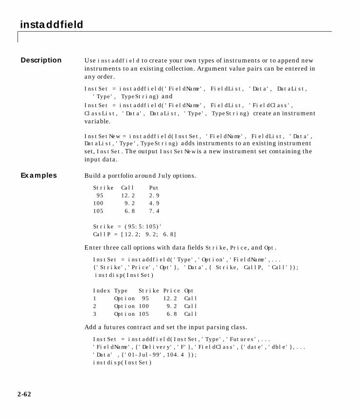
instaddfield
2-62
Description Use instaddfield to create your own types of instruments or to append newinstruments to an existing collection. Argument value pairs can be entered inany order.
InstSet = instaddfield('FieldName', FieldList, 'Data', DataList,'Type', TypeString) and
InstSet = instaddfield('FieldName', FieldList, 'FieldClass',ClassList, 'Data', DataList, 'Type', TypeString) create an instrumentvariable.
InstSetNew = instaddfield(InstSet, 'FieldName', FieldList, 'Data',DataList,'Type’,TypeString) adds instruments to an existing instrumentset, InstSet. The output InstSetNew is a new instrument set containing theinput data.
Examples Build a portfolio around July options.
Strike Call Put 95 12.2 2.9100 9.2 4.9105 6.8 7.4
Strike = (95:5:105)'CallP = [12.2; 9.2; 6.8]
Enter three call options with data fields Strike, Price, and Opt.
InstSet = instaddfield('Type','Option','FieldName',...{'Strike','Price','Opt'}, 'Data',{ Strike, CallP, 'Call'});instdisp(InstSet)
Index Type Strike Price Opt1 Option 95 12.2 Call2 Option 100 9.2 Call3 Option 105 6.8 Call
Add a futures contract and set the input parsing class.
InstSet = instaddfield(InstSet,'Type','Futures',...'FieldName',{'Delivery','F'},'FieldClass',{'date','dble'},...'Data' ,{'01-Jul-99',104.4 });instdisp(InstSet)

instaddfield
2-63
Index Type Strike Price Opt1 Option 95 12.2 Call2 Option 100 9.2 Call3 Option 105 6.8 Call
Index Type Delivery F4 Futures 01-Jul-1999 104.4
Add a put option.
FN = instfields(InstSet,'Type','Option')InstSet = instaddfield(InstSet,'Type','Option',...'FieldName',FN, 'Data',{105, 7.4, 'Put'});instdisp(InstSet)
Index Type Strike Price Opt1 Option 95 12.2 Call2 Option 100 9.2 Call3 Option 105 6.8 Call
Index Type Delivery F4 Futures 01-Jul-1999 104.4
Index Type Strike Price Opt5 Option 105 7.4 Put
Make a placeholder for another put.
InstSet = instaddfield(InstSet,'Type','Option',...'FieldName','Opt','Data','Put')instdisp(InstSet)
Index Type Strike Price Opt1 Option 95 12.2 Call2 Option 100 9.2 Call3 Option 105 6.8 Call
Index Type Delivery F4 Futures 01-Jul-1999 104.4

instaddfield
2-64
Index Type Strike Price Opt5 Option 105 7.4 Put6 Option NaN NaN Put
Add a cash instrument.
InstSet = instaddfield(InstSet, 'Type', 'TBill','FieldName','Price','Data',99)instdisp(InstSet)
Index Type Strike Price Opt1 Option 95 12.2 Call2 Option 100 9.2 Call3 Option 105 6.8 Call
Index Type Delivery F4 Futures 01-Jul-1999 104.4
Index Type Strike Price Opt5 Option 105 7.4 Put6 Option NaN NaN Put
Index Type Price7 TBill 99
See Also instdisp, instget, instgetcell, instsetfield
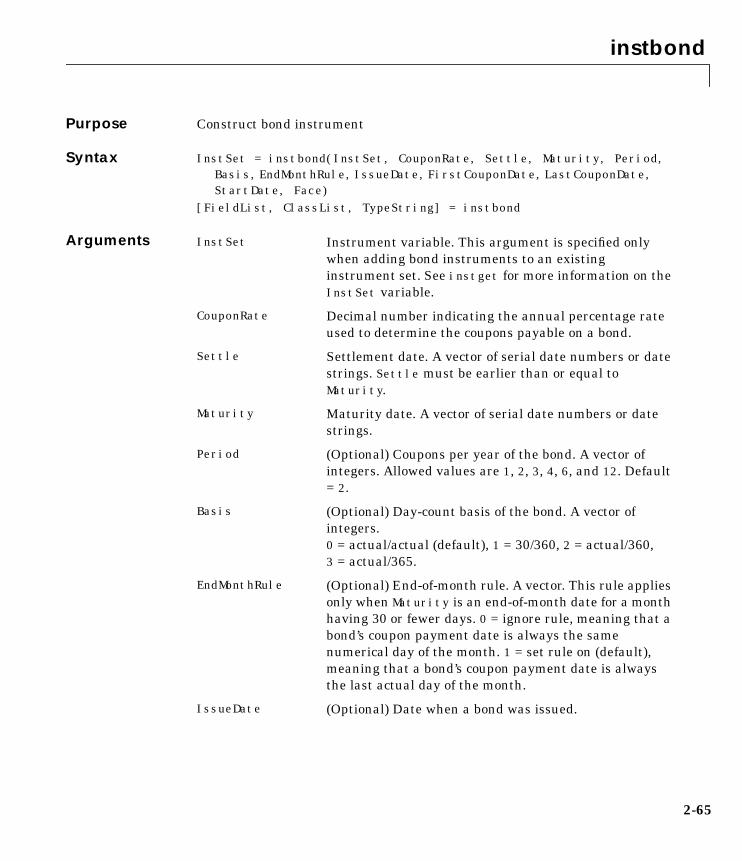
instbond
2-65
2instbondPurpose Construct bond instrument
Syntax InstSet = instbond(InstSet, CouponRate, Settle, Maturity, Period,Basis,EndMonthRule,IssueDate,FirstCouponDate,LastCouponDate,StartDate, Face)
[FieldList, ClassList, TypeString] = instbond
Arguments InstSet Instrument variable. This argument is specified onlywhen adding bond instruments to an existinginstrument set. See instget for more information on theInstSet variable.
CouponRate Decimal number indicating the annual percentage rateused to determine the coupons payable on a bond.
Settle Settlement date. A vector of serial date numbers or datestrings. Settle must be earlier than or equal toMaturity.
Maturity Maturity date. A vector of serial date numbers or datestrings.
Period (Optional) Coupons per year of the bond. A vector ofintegers. Allowed values are 1, 2, 3, 4, 6, and 12. Default= 2.
Basis (Optional) Day-count basis of the bond. A vector ofintegers.0 = actual/actual (default), 1 = 30/360, 2 = actual/360,3 = actual/365.
EndMonthRule (Optional) End-of-month rule. A vector. This rule appliesonly when Maturity is an end-of-month date for a monthhaving 30 or fewer days. 0 = ignore rule, meaning that abond’s coupon payment date is always the samenumerical day of the month. 1 = set rule on (default),meaning that a bond’s coupon payment date is alwaysthe last actual day of the month.
IssueDate (Optional) Date when a bond was issued.
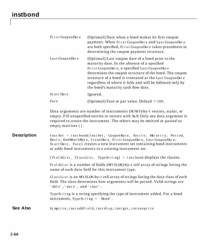
instbond
2-66
Data arguments are number of instruments (NINST)-by-1 vectors, scalar, orempty. Fill unspecified entries in vectors with NaN. Only one data argument isrequired to create the instrument. The others may be omitted or passed asempty matrices [].
Description InstSet = instbond(InstSet, CouponRate, Settle, Maturity, Period,Basis, EndMonthRule, IssueDate, FirstCouponDate, LastCouponDate,StartDate, Face) creates a new instrument set containing bond instrumentsor adds bond instruments to a existing instrument set.
[FieldList, ClassList, TypeString] = instbond displays the classes.
FieldList is a number of fields (NFIELDS)-by-1 cell array of strings listing thename of each data field for this instrument type.
ClassList is an NFIELDS-by-1 cell array of strings listing the data class of eachfield. The class determines how arguments will be parsed. Valid strings are'dble', 'date', and 'char'.
TypeString is a string specifying the type of instrument added. For a bondinstrument, TypeString = 'Bond'.
See Also hjmprice, instaddfield, instdisp, instget, intenvprice
FirstCouponDate (Optional) Date when a bond makes its first couponpayment. When FirstCouponDate and LastCouponDateare both specified, FirstCouponDate takes precedence indetermining the coupon payment structure.
LastCouponDate (Optional) Last coupon date of a bond prior to thematurity date. In the absence of a specifiedFirstCouponDate, a specified LastCouponDatedetermines the coupon structure of the bond. The couponstructure of a bond is truncated at the LastCouponDateregardless of where it falls and will be followed only bythe bond’s maturity cash flow date.
StartDate Ignored.
Face (Optional) Face or par value. Default = 100.

instcap
2-67
2instcapPurpose Construct cap instrument
Syntax InstSet = instcap(InstSet, Strike, Settle, Maturity, Reset, Basis,Principal)
[FieldList, ClassList, TypeString] = instcap
Arguments
Description InstSet = instcap(InstSet, Strike, Settle, Maturity, Reset, Basis,Principal) creates a new instrument set containing cap instruments or addscap instruments to an existing instrument set.
[FieldList, ClassList, TypeString] = instcap displays the classes.
FieldList is a number of fields (NFIELDS)-by-1 cell array of strings listing thename of each data field for this instrument type.
ClassList is an NFIELDS-by-1 cell array of strings listing the data class of eachfield. The class determines how arguments will be parsed. Valid strings are'dble', 'date', and 'char'.
TypeString is a string specifying the type of instrument added. For a capinstrument, TypeString = 'Cap'.
InstSet Instrument variable. This argument is specified onlywhen adding cap instruments to an existing instrumentset. See instget for more information on the InstSetvariable.
Strike Rate at which the cap is exercised, as a decimal number.
Settle Settlement date. Serial date number representing thesettlement date of the cap.
Maturity Serial date number representing the maturity date ofthe cap.
Reset (Optional) NINST-by-1 vector representing the resetfrequency per year. Default = 1.
Basis (Optional) NINST-by-1 vector representing the basis usedwhen annualizing the input forward rate tree. Default =0 (actual/actual).
Principal (Optional) The notional principal amount. Default = 100.

instcap
2-68
See Also hjmprice, instaddfield, instbond, instdisp, instfloor, instswap,intenvprice

instcf
2-69
2instcfPurpose Construct cash flow instrument
Syntax InstSet = instcf(InstSet, CFlowAmounts, CFlowDates, Settle, Basis)[FieldList, ClassList, TypeString] = instcf
Arguments
Only one data argument is required to create an instrument. Other argumentscan be omitted or passed as empty matrices []. Dates can be input as serialdate numbers or date strings.
Description InstSet = instcf(InstSet, CFlowAmounts, CFlowDates, Settle, Basis)creates a new instrument set from data arrays or adds instruments of typeCashFlow to an instrument set.
[FieldList, ClassList, TypeString] = instcf lists field meta-data for aninstrument of type CashFlow.
FieldList is a number of fields (NFIELDS)-by-1 cell array of strings listing thename of each data field for this instrument type.
InstSet Instrument variable. This argument is specified onlywhen adding cash flow instruments to an existinginstrument set. See instget for more information on theInstSet variable.
CFlowAmounts Number of instruments (NINST) by maximum number ofcash flows (MOSTCFS) matrix of cash flow amounts. Eachrow is a list of cash flow values for one instrument. If aninstrument has fewer than MOSTCFS cash flows, the endof the row is padded with NaNs.
CFlowDates NINST-by-MOSTCFSmatrix of cash flow dates. Each entrycontains the date of the corresponding cash flow inCFlowAmounts.
Settle Settlement date on which the cash flows are priced.
Basis (Optional) Day-count basis of the bond. A vector ofintegers.0 = actual/actual (default), 1 = 30/360, 2 = actual/360,3 = actual/365.

instcf
2-70
ClassList is an NFIELDS-by-1 cell array of strings listing the data class of eachfield. The class determines how arguments will be parsed. Valid strings are'dble', 'date', and 'char'.
TypeString specifies the type of instrument added, e.g.,TypeString = 'CashFlow'.
See Also hjmprice, instaddfield, instdisp, instget, intenvprice

instdelete
2-71
2instdeletePurpose Complement of a subset of instruments found by matching conditions
Syntax ISubSet = instdelete(InstSet, 'FieldName', FieldList, 'Data',DataList, 'Index', IndexSet, 'Type', TypeList)
Arguments
Argument value pairs can be entered in any order. The InstSet variable mustbe the first argument. 'FieldName' and 'Data' arguments must appeartogether or not at all.
Description The output argument ISubSet contains instruments not matching the inputcriteria. Instruments are deleted from ISubSet if all the Field, Index, and Typeconditions are met. An instrument meets an individual Field condition if thestored FieldName data matches any of the rows listed in the DataList for thatFieldName. See instfind for more examples on matching criteria.
InstSet Variable containing a collection of instruments.Instruments are classified by type; each type can havedifferent data fields. The stored data field is a row vectoror string for each instrument.
FieldList String or number of fields (NFIELDS)-by-1 cell array ofstrings listing the name of each data field to match withdata values.
DataList Number of values (NVALUES)-by-M array or NFIELDS-by-1cell array of acceptable data values for each field. Eachrow lists a data row value to search for in thecorresponding FieldList. The number of columns isarbitrary and matching will ignore trailing NaNs orspaces.
IndexSet (Optional) Number of instruments (NINST)-by-1 vectorrestricting positions of instruments to check for matches.The default is all indices available in the instrumentvariable.
TypeList (Optional) String or number of types (NTYPES)-by-1 cellarray of strings restricting instruments to match one ofTypeList types. The default is all types in theinstrument variable.

instdelete
2-72
Example Retrieve the instrument set variable ExampleInst from the data fileInstSetExamples.mat. The variable contains three types of instruments:Option, Futures, and TBill.
load InstSetExamples;instdisp(ExampleInst)
Index Type Strike Price Opt Contracts1 Option 95 12.2 Call 02 Option 100 9.2 Call 03 Option 105 6.8 Call 1000
Index Type Delivery F Contracts4 Futures 01-Jul-1999 104.4 -1000
Index Type Strike Price Opt Contracts5 Option 105 7.4 Put -10006 Option 95 2.9 Put 0
Index Type Price Maturity Contracts7 TBill 99 01-Jul-1999 6
Create a new variable, ISet, with all options deleted.
ISet = instdelete(ExampleInst, 'Type','Option');instdisp(ISet)
Index Type Delivery F Contracts1 Futures 01-Jul-1999 104.4 -1000
Index Type Price Maturity Contracts2 TBill 99 01-Jul-1999 6
See Also instaddfield, instfind, instget, instselect
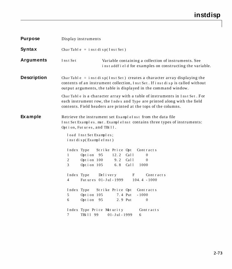
instdisp
2-73
2instdispPurpose Display instruments
Syntax CharTable = instdisp(InstSet)
Arguments
Description CharTable = instdisp(InstSet) creates a character array displaying thecontents of an instrument collection, InstSet. If instdisp is called withoutoutput arguments, the table is displayed in the command window.
CharTable is a character array with a table of instruments in InstSet. Foreach instrument row, the Index and Type are printed along with the fieldcontents. Field headers are printed at the tops of the columns.
Example Retrieve the instrument set ExampleInst from the data fileInstSetExamples.mat. ExampleInst contains three types of instruments:Option, Futures, and TBill.
load InstSetExamples;instdisp(ExampleInst)
Index Type Strike Price Opt Contracts1 Option 95 12.2 Call 02 Option 100 9.2 Call 03 Option 105 6.8 Call 1000
Index Type Delivery F Contracts4 Futures 01-Jul-1999 104.4 -1000
Index Type Strike Price Opt Contracts5 Option 105 7.4 Put -10006 Option 95 2.9 Put 0
Index Type Price Maturity Contracts7 TBill 99 01-Jul-1999 6
InstSet Variable containing a collection of instruments. Seeinstaddfield for examples on constructing the variable.

instdisp
2-74
See Also datestr in the Financial Toolbox User’s Guide
num2str in the online MATLAB reference
instaddfield, instget

instfields
2-75
2instfieldsPurpose List fields
Syntax FieldList = instfields(InstSet, 'Type', TypeList)
Arguments
Description FieldList = instfields(InstSet, 'Type', TypeList) retrieve list of fieldsstored in an instrument variable.
FieldList is a number of fields (NFIELDS)-by-1 cell array of strings listing thename of each data field corresponding to the listed types.
Example Retrieve the instrument set ExampleInst from the data fileInstSetExamples.mat. ExampleInst contains three types of instruments:Option, Futures, and TBill.
load InstSetExamples;instdisp(ExampleInst)
Index Type Strike Price Opt Contracts1 Option 95 12.2 Call 02 Option 100 9.2 Call 03 Option 105 6.8 Call 1000
Index Type Delivery F Contracts4 Futures 01-Jul-1999 104.4 -1000
Index Type Strike Price Opt Contracts5 Option 105 7.4 Put -10006 Option 95 2.9 Put 0
Index Type Price Maturity Contracts7 TBill 99 01-Jul-1999 6
InstSet Variable containing a collection of instruments.Instruments are classified by type; each type can havedifferent data fields. The stored data field is a row vectoror string for each instrument.
TypeList (Optional) String or number of types (NTYPES)-by-1 cellarray of strings listing the instrument types to query.

instfields
2-76
Get the fields listed for type 'Option'.
[FieldList, ClassList] = instfields(ExampleInst, 'Type',...'Option')
FieldList =
'Strike' 'Price' 'Opt' 'Contracts'
ClassList =
'dble' 'dble' 'char' 'dble'
Get the fields listed for types 'Option' and 'TBill' .
FieldList = instfields(ExampleInst, 'Type', {'Option', 'TBill'})
FieldList =
'Strike''Opt''Price''Maturity''Contracts'
Get all the fields listed in any type in the variable.
FieldList = instfields(ExampleInst)

instfields
2-77
FieldList =
'Delivery' 'F' 'Strike' 'Opt' 'Price' 'Maturity' 'Contracts'
See Also instdisp, instlength, insttypes
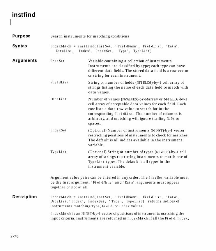
instfind
2-78
2instfindPurpose Search instruments for matching conditions
Syntax IndexMatch = instfind(InstSet, 'FieldName', FieldList, 'Data',DataList, 'Index', IndexSet, 'Type', TypeList)
Arguments
Argument value pairs can be entered in any order. The InstSet variable mustbe the first argument. 'FieldName' and 'Data' arguments must appeartogether or not at all.
Description IndexMatch = instfind(InstSet, 'FieldName', FieldList, 'Data',DataList,'Index', IndexSet, 'Type', TypeList) returns indices ofinstruments matching Type, Field, or Index values.
IndexMatch is an NINST-by-1 vector of positions of instruments matching theinput criteria. Instruments are returned in IndexMatch if all the Field, Index,
InstSet Variable containing a collection of instruments.Instruments are classified by type; each type can havedifferent data fields. The stored data field is a row vectoror string for each instrument.
FieldList String or number of fields (NFIELDS)-by-1 cell array ofstrings listing the name of each data field to match withdata values.
DataList Number of values (NVALUES)-by-M array or NFIELDS-by-1cell array of acceptable data values for each field. Eachrow lists a data row value to search for in thecorresponding FieldList. The number of columns isarbitrary, and matching will ignore trailing NaNs orspaces.
IndexSet (Optional) Number of instruments (NINST)-by-1 vectorrestricting positions of instruments to check for matches.The default is all indices available in the instrumentvariable.
TypeList (Optional) String or number of types (NTYPES)-by-1 cellarray of strings restricting instruments to match one ofTypeList types. The default is all types in theinstrument variable.

instfind
2-79
and Type conditions are met. An instrument meets an individual Fieldcondition if the stored FieldName data matches any of the rows listed in theDataList for that FieldName.
Example Retrieve the instrument set ExampleInst from the data fileInstSetExamples.mat. ExampleInst contains three types of instruments:Option, Futures, and TBill.
load InstSetExamples;instdisp(ExampleInst)
Index Type Strike Price Opt Contracts1 Option 95 12.2 Call 02 Option 100 9.2 Call 03 Option 105 6.8 Call 1000
Index Type Delivery F Contracts4 Futures 01-Jul-1999 104.4 -1000
Index Type Strike Price Opt Contracts5 Option 105 7.4 Put -10006 Option 95 2.9 Put 0
Index Type Price Maturity Contracts7 TBill 99 01-Jul-1999 6
Make a vector, Opt95, containing the indexes within ExampleInst of the optionsstruck at 95.
Opt95 = instfind(ExampleInst, 'FieldName','Strike','Data',’95’)
Opt95 =
1 6

instfind
2-80
Locate the futures and Treasury bill instruments within ExampleInst.
Types = instfind(ExampleInst,'Type',{'Futures';'TBill'})
Types =
4 7
See Also instaddfield, instget, instgetcell, instselect
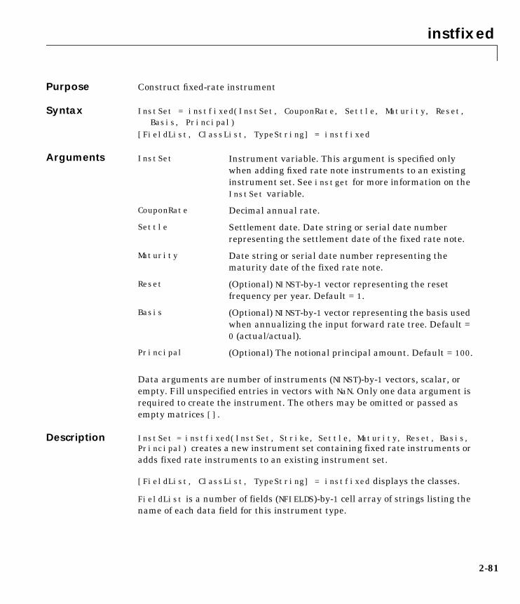
instfixed
2-81
2instfixedPurpose Construct fixed-rate instrument
Syntax InstSet = instfixed(InstSet, CouponRate, Settle, Maturity, Reset,Basis, Principal)
[FieldList, ClassList, TypeString] = instfixed
Arguments
Data arguments are number of instruments (NINST)-by-1 vectors, scalar, orempty. Fill unspecified entries in vectors with NaN. Only one data argument isrequired to create the instrument. The others may be omitted or passed asempty matrices [].
Description InstSet = instfixed(InstSet, Strike, Settle, Maturity, Reset, Basis,Principal) creates a new instrument set containing fixed rate instruments oradds fixed rate instruments to an existing instrument set.
[FieldList, ClassList, TypeString] = instfixed displays the classes.
FieldList is a number of fields (NFIELDS)-by-1 cell array of strings listing thename of each data field for this instrument type.
InstSet Instrument variable. This argument is specified onlywhen adding fixed rate note instruments to an existinginstrument set. See instget for more information on theInstSet variable.
CouponRate Decimal annual rate.
Settle Settlement date. Date string or serial date numberrepresenting the settlement date of the fixed rate note.
Maturity Date string or serial date number representing thematurity date of the fixed rate note.
Reset (Optional) NINST-by-1 vector representing the resetfrequency per year. Default = 1.
Basis (Optional) NINST-by-1 vector representing the basis usedwhen annualizing the input forward rate tree. Default =0 (actual/actual).
Principal (Optional) The notional principal amount. Default = 100.

instfixed
2-82
ClassList is an NFIELDS-by-1 cell array of strings listing the data class of eachfield. The class determines how arguments will be parsed. Valid strings are'dble', 'date', and 'char'.
TypeString is a string specifying the type of instrument added. For a fixed rateinstrument, TypeString = 'Fixed'.
See Also hjmprice, instaddfield, instbond, instcap, instdisp, instswap,intenvprice

instfloat
2-83
2instfloatPurpose Construct floating-rate instrument
Syntax InstSet = instfloat(InstSet, Spread, Settle, Maturity, Reset, Basis,Principal)
[FieldList, ClassList, TypeString] = instfloat
Arguments
Data arguments are number of instruments (NINST)-by-1 vectors, scalar, orempty. Fill unspecified entries in vectors with NaN. Only one data argument isrequired to create the instrument. The others may be omitted or passed asempty matrices [].
Description InstSet = instfloat(InstSet, Spread, Settle, Maturity, Reset, Basis,Principal) creates a new instrument set containing floating rate instrumentsor adds floating rate instruments to an existing instrument set.
[FieldList, ClassList, TypeString] = instfloat displays the classes.
FieldList is a number of fields (NFIELDS)-by-1 cell array of strings listing thename of each data field for this instrument type.
InstSet Instrument variable. This argument is specified onlywhen adding floating rate note instruments to anexisting instrument set. See instget for moreinformation on the InstSet variable.
Spread Number of basis points over the reference rate.
Settle Settlement date. Date string or serial date numberrepresenting the settlement date of the floating ratenote.
Maturity Date string or serial date number representing thematurity date of the floating rate note.
Reset (Optional) NINST-by-1 vector representing the resetfrequency per year. Default = 1.
Basis (Optional) NINST-by-1 vector representing the basis usedwhen annualizing the input forward rate tree. Default =0 (actual/actual).
Principal (Optional) The notional principal amount. Default = 100.

instfloat
2-84
ClassList is an NFIELDS-by-1 cell array of strings listing the data class of eachfield. The class determines how arguments will be parsed. Valid strings are'dble', 'date', and 'char'.
TypeString is a string specifying the type of instrument added. For a floatingrate instrument, TypeString = 'Float'.
See Also hjmprice, instaddfield, instbond, instcap, instdisp, instswap,intenvprice

instfloor
2-85
2instfloorPurpose Construct floor instrument
Syntax InstSet = instfloor(InstSet, Strike, Settle, Maturity, Reset, Basis,Principal)
[FieldList, ClassList, TypeString] = instfloor
Arguments
Description InstSet = instfloor(InstSet, Strike, Settle, Maturity, Reset, Basis,Principal) creates a new instrument set containing floor instruments or addsfloor instruments to an existing instrument set.
[FieldList, ClassList, TypeString] = instfloor displays the classes.
FieldList is a number of fields (NFIELDS)-by-1 cell array of strings listing thename of each data field for this instrument type.
InstSet Instrument variable. This argument is specified onlywhen adding floor instruments to an existing instrumentset. See instget for more information on the InstSetvariable.
Strike Rate at which the floor is exercised, as a decimalnumber.
Settle Settlement date. A vector of serial date numbers or datestrings. Settle must be earlier than or equal toMaturity.
Maturity Maturity date. A vector of serial date numbers or datestrings.
Reset (Optional) NINST-by-1 vector representing the resetfrequency per year. Default = 1.
Basis (Optional) Day-count basis of the bond. A vector ofintegers.0 = actual/actual (default), 1 = 30/360, 2 = actual/360,3 = actual/365.
Principal (Optional) The notional principal amount. Default = 100.

instfloor
2-86
ClassList is an NFIELDS-by-1 cell array of strings listing the data class of eachfield. The class determines how arguments will be parsed. Valid strings are'dble', 'date', and 'char'.
TypeString is a string specifying the type of instrument added. For a floorinstrument, TypeString = 'Floor'.
See Also hjmprice, instaddfield, instbond, instcap, instdisp, instswap,intenvprice
instget
2-87
2instgetPurpose Retrieve data from instrument variable
Syntax [Data_1, Data_2,...,Data_n] = instget(InstSet, 'FieldName',FieldList, 'Index', IndexSet, 'Type', TypeList)
Arguments
Parameter value pairs can be entered in any order. The InstSet variable mustbe the first argument.
Description [Data_1, Data_2,...,Data_n] = instget(InstSet, 'FieldName',FieldList, 'Index', IndexSet, 'Type', TypeList) retrieve data arraysfrom an instrument variable.
Data_1 is an NINST-by-M array of data contents for the first field in FieldList.Each row corresponds to a separate instrument in IndexSet. Unavailable datais returned as NaN or as spaces.
Data_n is an NINST-by-M array of data contents for the last field in FieldList.
InstSet Variable containing a collection of instruments.Instruments are classified by type; each type can havedifferent data fields. The stored data field is a row vectoror string for each instrument.
FieldList (Optional) String or number of fields (NFIELDS)-by-1 cellarray of strings listing the name of each data field tomatch with data values. FieldList entries can also beeither 'Type' or 'Index'; these return type strings andindex numbers respectively. The default is all fieldsavailable for the returned set of instruments.
IndexSet (Optional) Number of instruments (NINST)-by-1 vector ofpositions of instruments to work on. If TypeList is alsoentered, instruments referenced must be one ofTypeList types and contained in IndexSet. The defaultis all indices available in the instrument variable.
TypeList (Optional) String or number of types (NTYPES)-by-1 cellarray of strings restricting instruments to match one ofTypeList types. The default is all types in theinstrument variable.

instget
2-88
Examples Retrieve the instrument set ExampleInst from the data fileInstSetExamples.mat. ExampleInst contains three types of instruments:Option, Futures, and TBill.
load InstSetExamples;instdisp(ExampleInst)
Index Type Strike Price Opt Contracts1 Option 95 12.2 Call 02 Option 100 9.2 Call 03 Option 105 6.8 Call 1000
Index Type Delivery F Contracts4 Futures 01-Jul-1999 104.4 -1000
Index Type Strike Price Opt Contracts5 Option 105 7.4 Put -10006 Option 95 2.9 Put 0
Index Type Price Maturity Contracts7 TBill 99 01-Jul-1999 6
Extract the price from all instruments.
P = instget(ExampleInst,'FieldName','Price')
P =
12.2000 9.2000 6.8000 NaN 7.4000 2.9000 99.0000
Get all the prices and the number of contracts held.
[P,C] = instget(ExampleInst, 'FieldName', {'Price', 'Contracts'})
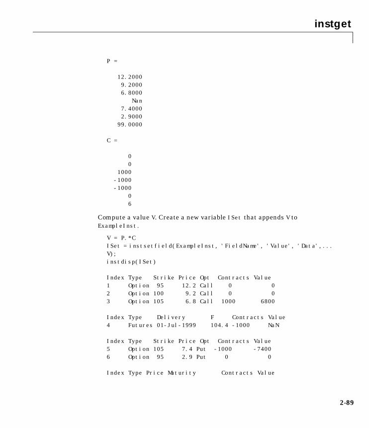
instget
2-89
P =
12.2000 9.2000 6.8000
Nan 7.4000 2.9000 99.0000
C =
0 0 1000 -1000 -1000 0 6
Compute a value V. Create a new variable ISet that appends V toExampleInst.
V = P.*CISet = instsetfield(ExampleInst, 'FieldName', 'Value', 'Data',...V);instdisp(ISet)
Index Type Strike Price Opt Contracts Value1 Option 95 12.2 Call 0 02 Option 100 9.2 Call 0 03 Option 105 6.8 Call 1000 6800
Index Type Delivery F Contracts Value4 Futures 01-Jul-1999 104.4 -1000 NaN
Index Type Strike Price Opt Contracts Value5 Option 105 7.4 Put -1000 -74006 Option 95 2.9 Put 0 0
Index Type Price Maturity Contracts Value

instget
2-90
7 TBill 99 01-Jul-1999 6 594
Look at only the instruments which have nonzero Contracts.
Ind = find(C ~= 0)
Ind =
3 4 5 7
Get the Type and Opt parameters from those instruments.( Only options havea stored 'Opt' field.)
[T,O] = instget(ExampleInst, 'Index', Ind, 'FieldName',...{'Type', 'Opt'})
T =
OptionFuturesOptionTBill
O =
Call
Put
Create a string report of holdings Type, Opt, and Value.
rstring = [T, O, num2str(V(Ind))]
rstring =
Option Call 6800Futures NaNOption Put -7400TBill 594

instget
2-91
See Also instaddfield, instdisp, instgetcell

instgetcell
2-92
2instgetcellPurpose Retrieve data and context from instrument variable
Syntax [DataList, FieldList, ClassList, IndexSet, TypeSet] =instgetcell(InstSet, 'FieldName', FieldList, 'Index', IndexSet,'Type', TypeList)
Arguments
Parameter value pairs can be entered in any order. The InstSet variable mustbe the first argument.
Description [DataList, FieldList, ClassList] = instgetcell(InstSet,'FieldName', FieldList, 'Index', IndexSet, 'Type', TypeList)retrieves data and context from an instrument variable.
DataList is an NFIELDS-by-1 cell array of data contents for each field. Each cellis an NINST-by-M array, where each row corresponds to a separate instrumentin IndexSet. Any data which is not available is returned as NaN or as spaces.
InstSet Variable containing a collection of instruments.Instruments are classified by type; each type can havedifferent data fields. The stored data field is a row vectoror string for each instrument.
FieldList (Optional) String or number of fields (NFIELDS)-by-1 cellarray of strings listing the name of each data field tomatch with data values. FieldList should not be eitherType or Index; these field names are reserved. Thedefault is all fields available for the returned set ofinstruments.
IndexSet (Optional) Number of instruments (NINST)-by-1 vector ofpositions of instruments to work on. If TypeList is alsoentered, instruments referenced must be one ofTypeList types and contained in IndexSet. The defaultis all indices available in the instrument variable.
TypeList (Optional) String or number of types (NTYPES)-by-1 cellarray of strings restricting instruments to match one ofTypeList types. The default is all types in theinstrument variable.

instgetcell
2-93
FieldList is an NFIELDS-by-1 cell array of strings listing the name of eachfield in DataList.
ClassList is an NFIELDS-by-1 cell array of strings listing the data class of eachfield. The class determines how arguments will be parsed. Valid strings are'dble', 'date', and 'char'.
IndexSet is an NINST-by-1 vector of positions of instruments returned inDataList.
TypeSet is an NINST-by-1 cell array of strings listing the type of eachinstrument row returned in DataList.
Example Retrieve the instrument set ExampleInst from the data fileInstSetExamples.mat. ExampleInst contains three types of instruments:Option, Futures, and TBill.
load InstSetExamples;instdisp(ExampleInst)
Index Type Strike Price Opt Contracts1 Option 95 12.2 Call 02 Option 100 9.2 Call 03 Option 105 6.8 Call 1000
Index Type Delivery F Contracts4 Futures 01-Jul-1999 104.4 -1000
Index Type Strike Price Opt Contracts5 Option 105 7.4 Put -10006 Option 95 2.9 Put 0
Index Type Price Maturity Contracts7 TBill 99 01-Jul-1999 6
Get the prices and contracts from all instruments.
FieldList = {'Price'; 'Contracts'}DataList = instgetcell(ExampleInst, 'FieldName', FieldList )P = DataList{1}C = DataList{2}
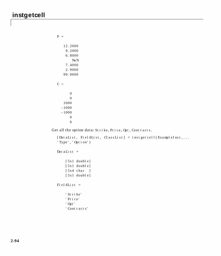
instgetcell
2-94
P =
12.2000 9.2000 6.8000 NaN 7.4000 2.9000 99.0000
C =
0 0 1000 -1000 -1000 0 6
Get all the option data: Strike, Price, Opt, Contracts.
[DataList, FieldList, ClassList] = instgetcell(ExampleInst,...'Type','Option')
DataList =
[5x1 double] [5x1 double] [5x4 char ] [5x1 double]
FieldList =
'Strike' 'Price' 'Opt' 'Contracts'
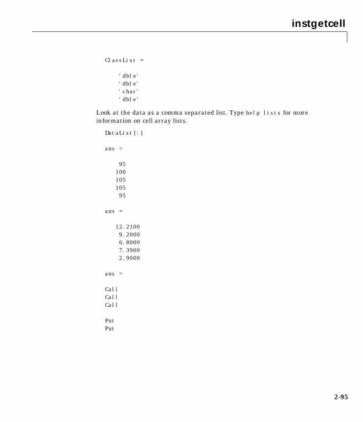
instgetcell
2-95
ClassList =
'dble' 'dble' 'char' 'dble'
Look at the data as a comma separated list. Type help lists for moreinformation on cell array lists.
DataList{:}
ans =
95 100 105 105 95
ans =
12.2100 9.2000 6.8000 7.3900 2.9000
ans =
CallCallCall
PutPut

instgetcell
2-96
ans =
0 0 100 -100 0
See Also instaddfield, instdisp, instget

instlength
2-97
2instlengthPurpose Count instruments
Syntax NInst = instlength(InstSet)
Arguments
Description NInst = instlength(InstSet) computes NInst, the number of instrumentscontained in the variable, InstSet.
See Also instdisp, instfields, insttypes
InstSet Variable containing a collection of instruments.Instruments are classified by type; each type can havedifferent data fields. The stored data field is a row vectoror string for each instrument.

instoptbnd
2-98
2instoptbndPurpose Construct bond option
Syntax InstSet = instoptbnd(InstSet, BondIndex, OptSpec, Strike,ExerciseDates, AmericanOpt )
[FieldList, ClassList, TypeString] = instoptbnd
Arguments InstSet Variable containing a collection of instruments.Instruments are classified by type; each type can havedifferent data fields. The stored data field is a row vectoror string for each instrument.
BondIndex Number of instruments (NINST)-by-1 vector of indicespointing to underlying instruments of Type 'Bond'which are also stored in InstSet. See instbond forinformation on specifying the bond data.
OptSpec NINST-by-1 list of string values 'Call' or 'Put'.
The interpretation of the Strike and ExerciseDates arguments dependsupon the setting of the AmericanOpt argument. If AmericanOpt = 0, NaN, or isunspecified, the option is a European or Bermuda option. If AmericanOpt = 1,the option is an American option.
Strike For a European or Bermuda option:NINST by number of strikes (NSTRIKES) matrix of strikeprice values. Each row is the schedule for one option. Ifan option has fewer than NSTRIKES exerciseopportunities, the end of the row is padded with NaNs.
For an American option:NINST-by-1 vector of strike price values for each option.
instoptbnd
2-99
Data arguments are NINST-by-1 vectors, scalar, or empty. Fill unspecifiedentries in vectors with NaN. Only one data argument is required to create theinstrument. The others may be omitted or passed as empty matrices [].
Description InstSet = instoptbnd(InstSet, BondIndex, OptSpec, Strike,ExerciseDates) specifies a European or Bermuda option.
InstSet = instoptbnd(InstSet, BondIndex, OptSpec, Strike,ExerciseDates, AmericanOpt) specifies an American option if AmericanOptis set to 1. If AmericanOpt is not set to 1, the function specifies a European orBermuda option.
FieldList is a number of fields (NFIELDS)-by-1 cell array of strings listing thename of each data field for this instrument type.
ClassList is an NFIELDS-by-1 cell array of strings listing the data class of eachfield. The class determines how arguments will be parsed. Valid strings are'dble', 'date', and 'char'.
TypeString is a string specifying the type of instrument added. For a bondinstrument, TypeString = 'Bond'.
See Also hjmprice, instadd, instdisp, instget
ExerciseDates For a European or Bermuda option:NINST-by-NSTRIKES matrix of exercise dates. Each row isthe schedule for one option. For a European option, thereis only one exercise date, the option expiry date.
For an American option:NINST-by-2 vector of exercise date boundaries. For eachinstrument, the option can be exercised on any coupondate between or including the pair of dates on that row.If only one non-NaN date is listed, or if ExerciseDates isNINST-by-1, the option can be exercised between theunderlying bond Settle and the single listed exercisedate.
instselect
2-100
2instselectPurpose Create instrument subset by matching conditions
Syntax InstSubSet = instselect(InstSet, 'FieldName', FieldList, 'Data',DataList, 'Index', IndexSet, 'Type', TypeList)
Arguments
Parameter value pairs can be entered in any order. The InstSet variable mustbe the first argument. 'FieldName' and 'Data' parameters must appeartogether or not at all. 'Index' and 'Type' parameters are each optional.
Description InstSubSet = instselect(InstSet, 'FieldName', FieldList, 'Data',DataList, 'Index', IndexSet, 'Type', TypeList) creates aninstrument subset (InstSubSet) from an existing set of instruments (InstSet).
InstSubSet is a variable containing instruments matching the input criteria.Instruments are returned in InstSubSet if all the Field, Index, and Type
InstSet Variable containing a collection of instruments.Instruments are classified by type; each type can havedifferent data fields. The stored data field is a row vectoror string for each instrument.
FieldList String or number of fields (NFIELDS)-by-1 cell array ofstrings listing the name of each data field to match withdata values.
DataList Number of values (NVALUES)-by-M array or NFIELDS-by-1cell array of acceptable data values for each field. Eachrow lists a data row value to search for in thecorresponding FieldList. The number of columns isarbitrary and matching will ignore trailing NaNs orspaces.
IndexSet (Optional) Number of instruments (NINST)-by-1 vectorrestricting positions of instruments to check for matches.The default is all indices available in the instrumentvariable.
TypeList (Optional) String or number of types (NTYPES)-by-1 cellarray of strings restricting instruments to match one ofTypeList types. The default is all types in theinstrument variable.

instselect
2-101
conditions are met. An instrument meets an individual Field condition if thestored FieldName data matches any of the rows listed in the DataList for thatFieldName. See instfind for examples on matching criteria.
Example Retrieve the instrument set ExampleInst from the data fileInstSetExamples.mat. The variable contains three types of instruments:Option, Futures, and TBill.
load InstSetExamplesinstdisp(ExampleInst)
Index Type Strike Price Opt Contracts1 Option 95 12.2 Call 02 Option 100 9.2 Call 03 Option 105 6.8 Call 1000
Index Type Delivery F Contracts4 Futures 01-Jul-1999 104.4 -1000
Index Type Strike Price Opt Contracts5 Option 105 7.4 Put -10006 Option 95 2.9 Put 0
Index Type Price Maturity Contracts7 TBill 99 01-Jul-1999 6
Make a new portfolio containing only options struck at 95.
Opt95 = instselect(ExampleInst, 'FieldName', 'Strike',...'Data', ’95’)
instdisp(Opt95)
Opt95 =
Index Type Strike Price Opt Contracts1 Option 95 12.2 Call 02 Option 95 2.9 Put 0
Make a new portfolio containing only futures and Treasury bills.

instselect
2-102
FutTBill = instselect(ExampleInst,'Type',{'Futures';'TBill'})
instdisp(FutTBill) =
Index Type Delivery F Contracts1 Futures 01-Jul-1999 104.4 -1000
Index Type Price Maturity Contracts2 TBill 99 01-Jul-1999 6
See Also instaddfield, instdelete, instfind, instget, instgetcell

instsetfield
2-103
2instsetfieldPurpose Add or reset data for existing instruments
Syntax InstSet = instsetfield(InstSet, 'FieldName', FieldList, 'Data',DataList)
InstSet = instsetfield(InstSet, 'FieldName', FieldList, 'Data',DataList, 'Index', IndexSet, 'Type', TypeList)
Arguments
Argument value pairs can be entered in any order.
Description instsetfield sets data for existing instruments in a collection variable.
InstSet = instsetfield(InstSet, 'FieldName', FieldList, 'Data',DataList) resets or adds fields to every instrument.
InstSet (Required) Variable containing a collection ofinstruments. Instruments are classified by type; eachtype can have different data fields. The stored data fieldis a row vector or string for each instrument. InstSetmust be the first argument in the list.
FieldList String or number of fields (NFIELDS)-by-1 cell array ofstrings listing the name of each data field. FieldListcannot be named with the reserved names Type orIndex.
DataList Number of instruments (NINST)-by-M array orNFIELDS-by-1 cell array of data contents for each field.Each row in a data array corresponds to a separateinstrument. Single rows are copied to apply to allinstruments to be worked on. The number of columns isarbitrary, and data will be padded along columns.
IndexSet NINST-by-1 vector of positions of instruments to work on.If TypeList is also entered, instruments referenced mustbe one of TypeList types and contained in IndexSet.
TypeList String or number of types (NTYPES)-by-1 cell array ofstrings restricting instruments worked on to match oneof TypeList types.

instsetfield
2-104
InstSet = instsetfield(InstSet, 'FieldName', FieldList, 'Data',DataList, 'Index', IndexSet, 'Type', TypeList) resets or adds fields toa subset of instruments.
The output InstSet is a new instrument set variable containing the input data.
Example Retrieve the instrument set ExampleInstSF from the data fileInstSetExamples.mat. ExampleInstSF contains three types of instruments:Option, Futures, and TBill.
load InstSetExamples;ISet = ExampleInstSF;instdisp(ISet)
Index Type Strike Price Opt1 Option 95 12.2 Call2 Option 100 9.2 Call3 Option 105 6.8 Call
Index Type Delivery F4 Futures 01-Jul-1999 104.4
Index Type Strike Price Opt5 Option 105 7.4 Put6 Option NaN NaN Put
Index Type Price7 TBill 99
Enter data for the option in Index 6: Price 2.9 for a Strike of 95.
ISet = instsetfield(ISet, 'Index',6,...'FieldName',{'Strike','Price'}, 'Data',{ 95 , 2.9 });instdisp(ISet)
Index Type Strike Price Opt1 Option 95 12.2 Call2 Option 100 9.2 Call3 Option 105 6.8 CallIndex Type Delivery F4 Futures 01-Jul-1999 104.4
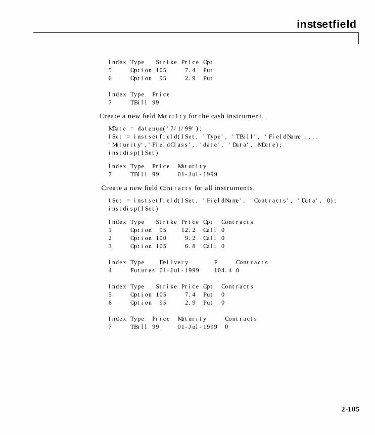
instsetfield
2-105
Index Type Strike Price Opt5 Option 105 7.4 Put6 Option 95 2.9 Put
Index Type Price7 TBill 99
Create a new field Maturity for the cash instrument.
MDate = datenum('7/1/99');ISet = instsetfield(ISet, 'Type', 'TBill', 'FieldName',...'Maturity','FieldClass', 'date', 'Data', MDate);instdisp(ISet)
Index Type Price Maturity7 TBill 99 01-Jul-1999
Create a new field Contracts for all instruments.
ISet = instsetfield(ISet, 'FieldName', 'Contracts', 'Data', 0);instdisp(ISet)
Index Type Strike Price Opt Contracts1 Option 95 12.2 Call 02 Option 100 9.2 Call 03 Option 105 6.8 Call 0
Index Type Delivery F Contracts4 Futures 01-Jul-1999 104.4 0
Index Type Strike Price Opt Contracts5 Option 105 7.4 Put 06 Option 95 2.9 Put 0
Index Type Price Maturity Contracts7 TBill 99 01-Jul-1999 0

instsetfield
2-106
Set the Contracts fields for some instruments.
ISet = instsetfield(ISet,'Index',[3; 5; 4; 7],...'FieldName','Contracts', 'Data', [1000; -1000; -1000; 6]);
instdisp(ISet)
Index Type Strike Price Opt Contracts1 Option 95 12.2 Call 02 Option 100 9.2 Call 03 Option 105 6.8 Call 1000
Index Type Delivery F Contracts4 Futures 01-Jul-1999 104.4 -1000
Index Type Strike Price Opt Contracts5 Option 105 7.4 Put -10006 Option 95 2.9 Put 0
Index Type Price Maturity Contracts7 TBill 99 01-Jul-1999 6
See Also instaddfield, instdisp, instget, instgetcell

instswap
2-107
2instswapPurpose Construct swap instrument
Syntax InstSet = instswap(InstSet, LegRate, Settle, Maturity, LegReset,Basis, Principal, LegType)
[FieldList, ClassList, TypeString] = instswap
Arguments InstSet Instrument variable. This argument is specified onlywhen adding a swap to an existing instrument set. Seeinstget for more information on the InstSet variable.
LegRate Number of instruments (NINST)-by-2 matrix, with eachrow defined as:[CouponRate Spread] or [Spread CouponRate]CouponRate is the decimal annual rate. Spread is thenumber of basis points over the reference rate. The firstcolumn represents the receiving leg, while the secondcolumn represents the paying leg.
Settle Settlement date. NINST-by-1 vector of serial datenumbers or date strings. Settle must be earlier than orequal to Maturity.
Maturity Maturity date. NINST-by-1 vector of dates representingthe maturity date for each swap.
LegReset (Optional) NINST-by-2 matrix representing the resetfrequency per year for each swap. Default = [1 1].
Basis (Optional) NINST-by-1 vector representing the basis usedwhen annualizing the input forward rate tree. Default =0 (actual/actual).
Principal (Optional) NINST-by-1 vector of the notional principalamounts. Default = 100.
LegType (Optional) NINST-by-2 matrix. Each row represents aninstrument. Each column indicates if the correspondingleg is fixed (1) or floating (0). This matrix defines theinterpretation of the values entered in LegRate. Defaultis [1,0] for each instrument.

instswap
2-108
Data arguments are number of instruments (NINST)-by-1 vectors, scalar, orempty. Fill unspecified entries in vectors with NaN. Only one data argument isrequired to create the instrument; the others may be omitted or passed asempty matrices [].
Description InstSet = instswap(InstSet, LegRate, Settle, Maturity, LegReset,Basis, Principal, LegType) creates a new instrument set containing swapinstruments or adds swap instruments to an existing instrument set.
[FieldList, ClassList, TypeString] = instswap displays the classes.
FieldList is a number of fields (NFIELDS)-by-1 cell array of strings listing thename of each data field for this instrument type.
ClassList is an NFIELDS-by-1 cell array of strings listing the data class of eachfield. The class determines how arguments will be parsed. Valid strings are'dble', 'date', and 'char'.
TypeString is a string specifying the type of instrument added. For a swapinstrument, TypeString = 'Swap'.
See Also hjmprice, instaddfield, instbond, instcap, instdisp, instfloor,intenvprice

insttypes
2-109
2insttypesPurpose List types
Syntax TypeList = insttypes(InstSet)
Arguments
Description TypeList = insttypes(InstSet) retrieves a list of types stored in aninstrument variable.
TypeList is a number of types (NTYPES)-by-1 cell array of strings listing theType of instruments contained in the variable.
Example Retrieve the instrument set variable ExampleInst from the data fileInstSetExamples.mat. ExampleInst contains three types of instruments:Option, Futures, and TBill.
load InstSetExamples;instdisp(ExampleInst)
Index Type Strike Price Opt Contracts1 Option 95 12.2 Call 02 Option 100 9.2 Call 03 Option 105 6.8 Call 1000
Index Type Delivery F Contracts4 Futures 01-Jul-1999 104.4 -1000
Index Type Strike Price Opt Contracts5 Option 105 7.4 Put -10006 Option 95 2.9 Put 0
Index Type Price Maturity Contracts7 TBill 99 01-Jul-1999 6
InstSet Variable containing a collection of instruments.Instruments are classified by type; each type can havedifferent data fields. The stored data field is a row vectoror string for each instrument.

insttypes
2-110
List all of the types included in ExampleInst.
TypeList = insttypes(ExampleInst)TypeList = 'Futures' 'Option' 'TBill'
See Also instdisp, instfields, instlength

intenvget
2-111
2intenvgetPurpose Obtain properties of an interest term structure
Syntax ParameterValue = intenvget(RateSpec, 'ParameterName')
Arguments
Description ParameterValue = intenvget(RateSpec,'ParameterName') obtains thevalue of the named parameter ParameterName extracted from RateSpec.
Example Use intenvset to set the interest rate structure.
RateSpec = intenvset('Rates', 0.05, 'StartDates',...'20-Jan-2000', 'EndDates', '20-Jan-2001')
Now use intenvget to extract the values from RateSpec.
[R, RateSpec] = intenvget(RateSpec, 'Rates')
R =
0.0500
RateSpec A structure encapsulating the properties of an interestrate structure. See intenvset for information oncreating RateSpec.
ParameterName String indicating the parameter name to be accessed.The value of the named parameter is extracted from thestructure RateSpec. It is sufficient to type only theleading characters that uniquely identify the parameter.Case is ignored for parameter names.

intenvget
2-112
RateSpec =
FinObj: 'RateSpec'Compounding: 2Disc: 0.9518Rates: 0.0500EndTimes: 2StartTimes: 0EndDates: 730871StartDates: 730505ValuationDate: 730505Basis: 0EndMonthRule: 1
See Also intenvset

intenvprice
2-113
2intenvpricePurpose Price fixed income instruments by a set of zero curves
Syntax Price = intenvprice(RateSpec, InstSet)
Arguments
Description Price = intenvprice(RateSpec, InstSet) computes arbitrage free pricesfor instruments against a set of zero coupon bond rate curves.
Price is a number of instruments (NINST) by number of curves (NUMCURVES)matrix of prices of each instrument. If an instrument cannot be priced, a NaN isreturned in that entry.
intenvprice handles the following instrument types: 'Bond', 'CashFlow','Fixed', 'Float', 'Swap'. See instadd for information about constructingdefined types.
See single-type pricing functions to retrieve pricing information.
Example Load the zero curves and instruments from a data file.
load deriv.matinstdisp(ZeroInstSet)
RateSpec A structure encapsulating the properties of an interestrate structure. See intenvset for information oncreating RateSpec.
InstSet Variable containing a collection of instruments.Instruments are categorized by type; each type can havedifferent data fields. The stored data field is a row vectoror string for each instrument.
bondbyzero Price bonds by a set of zero curves.
cfbyzero Price arbitrary cash flow instrument by a set of zero curves.
fixedbyzero Fixed rate note prices by zero curves.
floatbyzero Floating rate note prices by zero curves.
swapbyzero Swap prices by a set of zero curves.

intenvprice
2-114
Price = intenvprice(ZeroRateSpec, ZeroInstSet)
Price =
105.7678 107.6912 105.7678 100.5768 5.1910
See Also hjmprice, hjmsens, instadd, intenvsens, intenvset,
Index Type CouponRate Settle Maturity Period ... Name Quantity1 Bond 0.04 01-Jan-2000 01-Jan-2003 1 4% bond 1002 Bond 0.04 01-Jan-2000 01-Jan-2004 2 4% bond 50
Index Type CouponRate Settle Maturity FixedReset Basis Principal Name Quantity3 Fixed 0.04 01-Jan-2000 01-Jan-2003 1 NaN NaN 4% Fixed 80
Index Type Spread Settle Maturity FloatReset Basis Principal Name Quantity4 Float 20 01-Jan-2000 01-Jan-2003 1 NaN NaN 20BP Float 8
Index Type LegRate Settle Maturity LegReset Basis Principal LegType Name Quantity5 Swap 0.04 01-Jan-2000 01-Jan-2003 1 1 NaN NaN NaN 4%/20BP Swap 10
intenvsens
2-115
2intenvsensPurpose Instrument price and sensitivities by a set of zero curves
Syntax [Delta, Gamma, Price] = intenvsens(RateSpec, InstSet)
Arguments
Description [Delta, Gamma, Price] = intenvsens(RateSpec, InstSet) computesdollar prices and price sensitivities for instruments using a zero coupon bondrate term structure.
Delta is a number of instruments (NINST) by number of curves (NUMCURVES)matrix of deltas, representing the rate of change of instrument prices withrespect to shifts in the observed forward yield curve. Delta is computed byfinite differences.
Gamma is an NINST-by-NUMCURVES matrix of gammas, representing the rate ofchange of instrument deltas with respect to shifts in the observed forward yieldcurve. Gamma is computed by finite differences.
Note Both sensitivities are returned as dollar sensitivities. To find theper-dollar sensitivities, divide by the respective instrument price.
Price is an NINST-by-NUMCURVES matrix of prices of each instrument. If aninstrument cannot be priced, a NaN is returned.
intenvsens handles the following instrument types: 'Bond', 'CashFlow','Fixed', 'Float', 'Swap'. See instadd for information about constructingdefined types.
Example Load the tree and instruments from a data file.
RateSpec A structure encapsulating the properties of an interestrate structure. See intenvset for information oncreating RateSpec.
InstSet Variable containing a collection of instruments.Instruments are categorized by type; each type can havedifferent data fields. The stored data field is a row vectoror string for each instrument.

intenvsens
2-116
load deriv.matinstdisp(ZeroInstSet)
[Delta, Gamma] = intenvsens(ZeroRateSpec, ZeroInstSet)
Delta =
-299.7172 -395.8516 -299.7172 -1.1237 -298.5935
Gamma =
1.0e+003 *
1.1603 1.9014 1.1603 0.0037 1.1567
See Also hjmprice, hjmsens, instadd, intenvprice, intenvset
Index Type CouponRate Settle Maturity Period ... Name Quantity1 Bond 0.04 01-Jan-2000 01-Jan-2003 1 4% bond 1002 Bond 0.04 01-Jan-2000 01-Jan-2004 2 4% bond 50
Index Type CouponRate Settle Maturity FixedReset Basis Principal Name Quantity3 Fixed 0.04 01-Jan-2000 01-Jan-2003 1 NaN NaN 4% Fixed 80
Index Type Spread Settle Maturity FloatReset Basis Principal Name Quantity4 Float 20 01-Jan-2000 01-Jan-2003 1 NaN NaN 20BP Float 8
Index Type LegRate Settle Maturity LegReset Basis Principal LegType Name Quantity5 Swap 0.04 01-Jan-2000 01-Jan-2003 1 1 NaN NaN NaN 4%/20BP Swap 10

intenvset
2-117
2intenvsetPurpose Set properties of interest rate environment
Syntax [RateSpec, RateSpecOld] = intenvset(RateSpec, 'Parameter1', Value1,'Parameter2', Value2, ...)
[RateSpec, RateSpecOld] = intenvsetintenvset
Arguments
Parameters may be chosen from the table below and specified in any order.
RateSpec (Optional) An existing interest rate specificationstructure to be changed, probably created from aprevious call to intenvset.
Compounding Scalar value representing the rate at which the inputzero rates were compounded when annualized. Default =2. This argument determines the formula for thediscount factors:Compounding = 1, 2, 3, 4, 6, 12Disc = (1 + Z/F)^(-T), where F is the compounding
frequency, Z is the zero rate, and T is the time inperiodic units, e.g. T = F is one year.
Compounding = 365Disc = (1 + Z/F)^(-T), where F is the number of days
in the basis year and T is a number of dayselapsed computed by basis.
Compounding = -1Disc = exp(-T*Z), where T is time in years.
Disc Number of points (NPOINTS) by number of curves(NCURVES) matrix of unit bond prices over investmentintervals from StartDates, when the cash flow is valued,to EndDates, when the cash flow is received.
Rates Number of points (NPOINTS) by number of curves(NCURVES) matrix of rates in decimal form. Forexample, 5% is 0.05 in Rates. Rates are the yields overinvestment intervals from StartDates, when the cashflow is valued, to EndDates, when the cash flow isreceived.

intenvset
2-118
It is sufficient to type only the leading characters that uniquely identify theparameter. Case is ignored for parameter names.
When creating a new RateSpec, the set of parameters passed to intenvsetmust include StartDates, EndDates, and either Rates or Disc.
Call intenvset with no input or output arguments to display a list ofparameter names and possible values.
Description [RateSpec, RateSpecOld] = intenvset(RateSpec, 'Parameter1', Value1,'Parameter2', Value2, ...) creates an interest term structure (RateSpec)in which the input argument list is specified as parameter name /parametervalue pairs. The parameter name portion of the pair must be recognized as avalid field of the output structure RateSpec; the parameter value portion of thepair is then assigned to its paired field.
EndDates NPOINTS-by-1 vector or scalar of serial maturity datesending the interval to discount over.
StartDates NPOINTS-by-1 vector or scalar of serial dates starting theinterval to discount over.Default = ValuationDate.
ValuationDate (Optional) Scalar value in serial date number formrepresenting the observation date of the investmenthorizons entered in StartDates and EndDates. Default =min(StartDates).
Basis (Optional) Day-count basis of the bond. A vector ofintegers.0 = actual/actual (default), 1 = 30/360, 2 = actual/360,3 = actual/365.
EndMonthRule (Optional) End-of-month rule. A vector. This rule appliesonly when Maturity is an end-of-month date for a monthhaving 30 or fewer days. 0 = ignore rule, meaning that abond’s coupon payment date is always the samenumerical day of the month. 1 = set rule on (default),meaning that a bond’s coupon payment date is alwaysthe last actual day of the month.
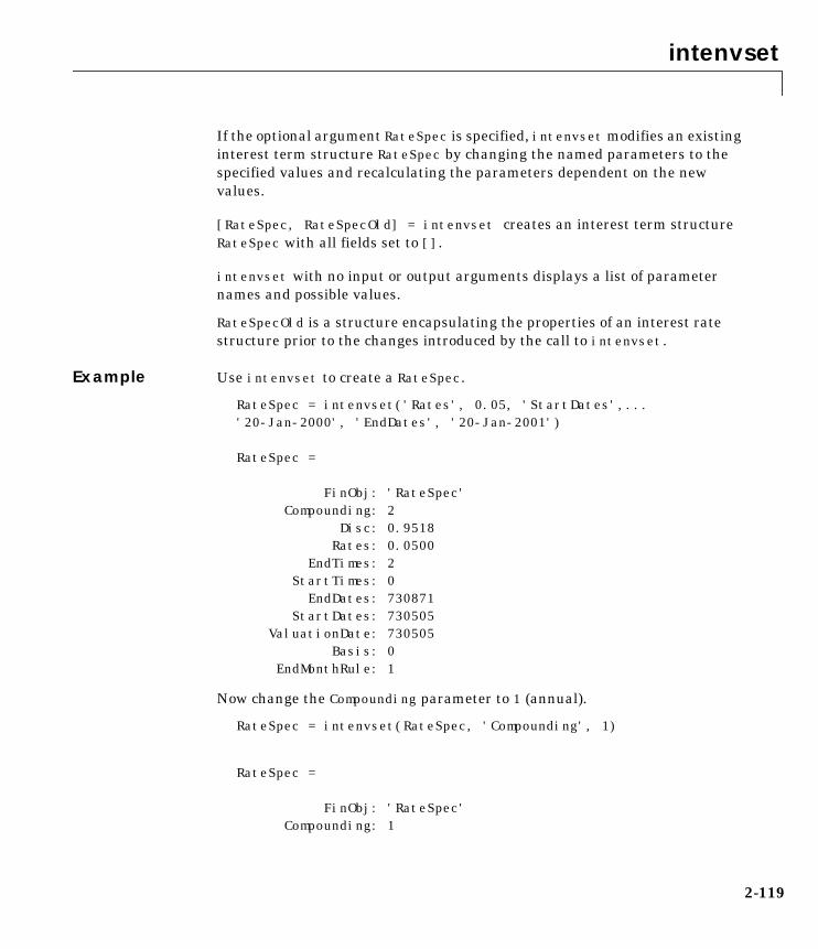
intenvset
2-119
If the optional argument RateSpec is specified, intenvset modifies an existinginterest term structure RateSpec by changing the named parameters to thespecified values and recalculating the parameters dependent on the newvalues.
[RateSpec, RateSpecOld] = intenvset creates an interest term structureRateSpec with all fields set to [].
intenvset with no input or output arguments displays a list of parameternames and possible values.
RateSpecOld is a structure encapsulating the properties of an interest ratestructure prior to the changes introduced by the call to intenvset.
Example Use intenvset to create a RateSpec.
RateSpec = intenvset('Rates', 0.05, 'StartDates',...'20-Jan-2000', 'EndDates', '20-Jan-2001')
RateSpec =
FinObj: 'RateSpec' Compounding: 2 Disc: 0.9518 Rates: 0.0500 EndTimes: 2 StartTimes: 0 EndDates: 730871 StartDates: 730505 ValuationDate: 730505 Basis: 0 EndMonthRule: 1
Now change the Compounding parameter to 1 (annual).
RateSpec = intenvset(RateSpec, 'Compounding', 1)
RateSpec =
FinObj: 'RateSpec' Compounding: 1
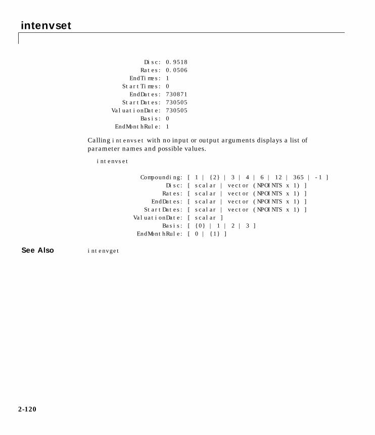
intenvset
2-120
Disc: 0.9518 Rates: 0.0506 EndTimes: 1 StartTimes: 0 EndDates: 730871 StartDates: 730505 ValuationDate: 730505 Basis: 0 EndMonthRule: 1
Calling intenvset with no input or output arguments displays a list ofparameter names and possible values.
intenvset
Compounding: [ 1 | {2} | 3 | 4 | 6 | 12 | 365 | -1 ] Disc: [ scalar | vector (NPOINTS x 1) ] Rates: [ scalar | vector (NPOINTS x 1) ] EndDates: [ scalar | vector (NPOINTS x 1) ] StartDates: [ scalar | vector (NPOINTS x 1) ] ValuationDate: [ scalar ] Basis: [ {0} | 1 | 2 | 3 ] EndMonthRule: [ 0 | {1} ]
See Also intenvget
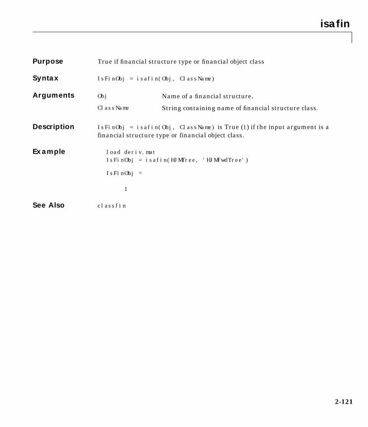
isafin
2-121
2isafinPurpose True if financial structure type or financial object class
Syntax IsFinObj = isafin(Obj, ClassName)
Arguments
Description IsFinObj = isafin(Obj, ClassName) is True (1) if the input argument is afinancial structure type or financial object class.
Example load deriv.matIsFinObj = isafin(HJMTree, 'HJMFwdTree')
IsFinObj =
1
See Also classfin
Obj Name of a financial structure.
ClassName String containing name of financial structure class.

mkbush
2-122
2mkbushPurpose Create bushy tree
Syntax [Tree, NumStates] = mkbush(NumLevels, NumChild, NumPos, Trim,NodeVal)
Arguments
Description [Tree, NumStates] = mkbush(NumLevels, NumChild, NumPos, Trim,NodeVal) creates a bushy tree Tree with initial values NodeVal at each node.NumStates is a 1-by-NUMLEVELS vector containing the number of state vectors ineach level.
Example Create a tree with four time levels, two branches per node, and a vector of threeelements in each node with each element initialized to NaN.
Tree = mkbush(4, 2, 3)
See Also bushpath, bushshape
NumLevels Number of time levels of the tree.
NumChild 1 by number of levels (NUMLEVELS) vector with number ofbranches (children) of the nodes in each level.
NumPos 1-by-NUMLEVELS vector containing the length of the statevectors in each time level.
Trim Scalar 0 or 1. If Trim = 1, NumPos decreases by 1 whenmoving from one time level to the next. Otherwise, ifTrim = 0 (Default), NumPos does not decrease.
NodeVal Initial value at each node of the tree. Default = NaN.

mmktbyhjm
2-123
2mmktbyhjmPurpose Create money market tree
Syntax MMktTree = mmktbyhjm(HJMTree)
Arguments
Description MMktTree = mmktbyhjm(HJMTree) creates a money market tree from a forwardrate tree structure created by hjmtree.
Example load deriv.mat;MMktTree = mmktbyhjm(HJMTree);treeviewer(MMktTree)
See Also hjmtree
HJMTree Forward rate tree structure created by hjmtree.

optbndbyhjm
2-124
2optbndbyhjmPurpose Price bond option by HJM interest rate tree
Syntax [Price, PriceTree] = optbndbyhjm(HJMTree, OptSpec, Strike,ExerciseDates, AmericanOpt, CouponRate, Settle, Maturity,Period, Basis, EndMonthRule, IssueDate, FirstCouponDate,LastCouponDate, StartDate, Face, Options)
Arguments HJMTree Forward rate tree structure created by hjmtree.
OptSpec Number of instruments (NINST)-by-1 cell array of stringvalues 'Call' or 'Put'.
Strike For a European or Bermuda option:NINST by number of strikes (NSTRIKES) matrix of strikeprice values. Each row is the schedule for one option. Ifan option has fewer than NSTRIKES exerciseopportunities, the end of the row is padded with NaNs.
For an American option:NINST-by-1 vector of strike price values for each option.
ExerciseDates For a European or Bermuda option:NINST-by-NSTRIKES matrix of exercise dates. Each row isthe schedule for one option. A European option has onlyone exercise date, the option expiry date.
For an American option:NINST-by-2 vector of exercise date boundaries. For eachinstrument, the option can be exercised on any coupondate between or including the pair of dates on that row.If only one non-NaN date is listed, or if ExerciseDates isNINST-by-1, the option can be exercised between theunderlying bond Settle and the single listed exercisedate.
AmericanOpt NINST-by-1 vector of flags: 0 (European/Bermuda) or 1(American)
CouponRate Decimal annual rate.

optbndbyhjm
2-125
Settle Settlement date. A vector of serial date numbers or datestrings. Settle must be earlier than or equal toMaturity.
Maturity Maturity date. A vector of serial date numbers or datestrings.
Period (Optional) Coupons per year of the bond. A vector ofintegers. Allowed values are 1, 2, 3, 4, 6, and 12. Default= 2.
Basis (Optional) Day-count basis of the bond. A vector ofintegers.0 = actual/actual (default), 1 = 30/360, 2 = actual/360,3 = actual/365.
EndMonthRule (Optional) End-of-month rule. A vector. This rule appliesonly when Maturity is an end-of-month date for a monthhaving 30 or fewer days. 0 = ignore rule, meaning that abond’s coupon payment date is always the samenumerical day of the month. 1 = set rule on (default),meaning that a bond’s coupon payment date is alwaysthe last actual day of the month.
IssueDate (Optional) Date when a bond was issued.
FirstCouponDate Date when a bond makes its first coupon payment. WhenFirstCouponDate and LastCouponDate are bothspecified, FirstCouponDate takes precedence indetermining the coupon payment structure.
LastCouponDate Last coupon date of a bond prior to the maturity date. Inthe absence of a specified FirstCouponDate, a specifiedLastCouponDate determines the coupon structure of thebond. The coupon structure of a bond is truncated at theLastCouponDate regardless of where it falls and will befollowed only by the bond’s maturity cash flow date.
StartDate Ignored.

optbndbyhjm
2-126
The Settle date for every bond is set to the ValuationDate of the HJM tree.The bond argument Settle is ignored.
Description optbondbyhjm is a dynamic programming subroutine for hjmprice.
Price is an NINST-by-1 matrix of expected prices at time 0.
PriceTree is a tree structure with a vector of instrument prices at each node.
Examples Using the HJM forward rate tree in the deriv.mat file, price a European calloption on a 4% bond with a strike of 101. The exercise date for the option is Jan.01, 2003. The settle date for the bond is Jan. 01, 2000, and the maturity dateis Jan. 01, 2004.
Load the file deriv.mat, which provides HJMTree. HJMTree contains the timeand forward rate information needed to price the bond.
load deriv
Use optbondbyhjm to compute the Price of the option.
Price = optbndbyhjm(HJMTree,'Call','101','01-Jan-2003',...'0','0.04','01-Jan-2000','01-Jan-2004')Warning: Not all cash flows are aligned with the tree. Result willbe approximated.
Price =
7.3217
See Also hjmprice, hjmtree, instoptbnd
Face Face value. Default is 100.
Options (Optional) Derivatives pricing options structure createdwith derivset.

rate2disc
2-127
2rate2discPurpose Discounting factors from interest rates
Syntax Usage 1: Interval points input as times in periodic units
Disc = rate2disc(Compounding, Rates, EndTimes, StartTimes)
Usage 2: ValuationDate passed and interval points input as dates
[Disc, EndTimes, StartTimes] = rate2disc(Compounding, Rates,EndDates, StartDates, ValuationDate)
Arguments Compounding Scalar value representing the rate at which the inputzero rates were compounded when annualized. Thisargument determines the formula for the discountfactors:Compounding = 1, 2, 3, 4, 6, 12Disc = (1 + Z/F)^(-T), where F is the compounding
frequency, Z is the zero rate, and T is the time inperiodic units, e.g. T = F is one year.
Compounding = 365Disc = (1 + Z/F)^(-T), where F is the number of days
in the basis year and T is a number of dayselapsed computed by basis.
Compounding = -1Disc = exp(-T*Z), where T is time in years.
Rates Number of points (NPOINTS) by number of curves(NCURVES) matrix of rates in decimal form. Forexample, 5% is 0.05 in Rates. Rates are the yields overinvestment intervals from StartTimes, when the cashflow is valued, to EndTimes, when the cash flow isreceived.
EndTimes NPOINTS-by-1 vector or scalar of times in periodic unitsending the interval to discount over.
StartTimes (Optional) NPOINTS-by-1 vector or scalar of times inperiodic units starting the interval to discount over.Default = 0.

rate2disc
2-128
Description Disc = rate2disc(Compounding, Rates, EndTimes, StartTimes) and
[Disc, EndTimes, StartTimes] = rate2disc(Compounding, Rates,EndDates, StartDates, ValuationDate) convert interest rates to cash flowdiscounting factors. rate2disc computes the discounts over a series of NPOINTStime intervals given the annualized yield over those intervals. NCURVESdifferent rate curves can be translated at once if they have the same timestructure. The time intervals can represent a zero curve or a forward curve.
Disc is an NPOINTS-by-NCURVES column vector of discount factors in decimalform representing the value at time StartTime of a unit cash flow received attime EndTime.
StartTimes is an NPOINTS-by-1 column vector of times starting the interval todiscount over, measured in periodic units.
EndTimes is an NPOINTS-by-1 column vector of times ending the interval todiscount over, measured in periodic units.
If Compounding = 365 (daily), StartTimes and EndTimes are measured in days.The arguments otherwise contain values, T, computed from SIA semiannualtime factors, Tsemi, by the formula T = Tsemi/2*F, where F is the compoundingfrequency.
The investment intervals can be specified either with input times (Usage 1) orwith input dates (Usage 2). Entering ValuationDate invokes the dateinterpretation; omitting ValuationDate invokes the default timeinterpretations.
EndDates NPOINTS-by-1 vector or scalar of serial maturity datesending the interval to discount over.
StartDates (Optional) NPOINTS-by-1 vector or scalar of serial datesstarting the interval to discount over.Default = ValuationDate.
ValuationDate Scalar value in serial date number form representing theobservation date of the investment horizons entered inStartDates and EndDates. Required in Usage 2. Omittedor passed as an empty matrix to invoke Usage 1.

rate2disc
2-129
Example Example 1. Compute discounts from a zero curve at six months, 12 months, and24 months. The time to the cash flows is 1, 2, and 4. We are computing thepresent value (at time 0) of the cash flows.
Compounding = 2;Rates = [0.05; 0.06; 0.065];EndTimes = [1; 2; 4];Disc = rate2disc(Compounding, Rates, EndTimes)
Disc =0.97560.94260.8799
Example 2. Compute discounts from a zero curve at six months, 12 months,and 24 months. Use dates to specify the ending time horizon.
Compounding = 2;Rates = [0.05; 0.06; 0.065];EndDates = ['10/15/97'; '04/15/98'; '04/15/99'];ValuationDate = '4/15/97';Disc = rate2disc(Compounding, Rates, EndDates, [], ValuationDate)
Disc =0.97560.94260.8799
Example 3. Compute discounts from the one-year forward rates beginning now,in six months, and in 12 months. Use monthly compounding. The times to thecash flows are 12, 18, 24, and the forward times are 0, 6, 12.
Compounding = 12;Rates = [0.05; 0.04; 0.06];EndTimes = [12; 18; 24];StartTimes = [0; 6; 12];Disc = rate2disc(Compounding, Rates, EndTimes, StartTimes)

rate2disc
2-130
Disc =0.95130.96090.9419
See Also disc2rate, ratetimes
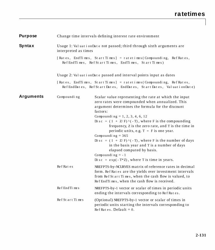
ratetimes
2-131
2ratetimesPurpose Change time intervals defining interest rate environment
Syntax Usage 1: ValuationDate not passed; third through sixth arguments areinterpreted as times
[Rates, EndTimes, StartTimes] = ratetimes(Compounding, RefRates,RefEndTimes, RefStartTimes, EndTimes, StartTimes)
Usage 2: ValuationDate passed and interval points input as dates
[Rates, EndTimes, StartTimes] = ratetimes(Compounding, RefRates,RefEndDates, RefStartDates, EndDates, StartDates, ValuationDate)
Arguments Compounding Scalar value representing the rate at which the inputzero rates were compounded when annualized. Thisargument determines the formula for the discountfactors:Compounding = 1, 2, 3, 4, 6, 12Disc = (1 + Z/F)^(-T), where F is the compounding
frequency, Z is the zero rate, and T is the time inperiodic units, e.g. T = F is one year.
Compounding = 365Disc = (1 + Z/F)^(-T), where F is the number of days
in the basis year and T is a number of dayselapsed computed by basis.
Compounding = -1Disc = exp(-T*Z), where T is time in years.
RefRates NREFPTS-by-NCURVES matrix of reference rates in decimalform. RefRates are the yields over investment intervalsfrom RefStartTimes, when the cash flow is valued, toRefEndTimes, when the cash flow is received.
RefEndTimes NREFPTS-by-1 vector or scalar of times in periodic unitsending the intervals corresponding to RefRates.
RefStartTimes (Optional) NREFPTS-by-1 vector or scalar of times inperiodic units starting the intervals corresponding toRefRates. Default = 0.

ratetimes
2-132
Description [Rates, EndTimes, StartTimes] = ratetimes(Compounding, RefRates,RefEndTimes, RefStartTimes, EndTimes, StartTimes) and[Rates, EndTimes, StartTimes] = ratetimes(Compounding, RefRates,RefEndDates, RefStartDates, EndDates, StartDates, ValuationDate)change time intervals defining an interest rate environment.
ratetimes takes an interest rate environment defined by yields over onecollection of time intervals and computes the yields over another set of timeintervals. The zero rate is assumed to be piecewise linear in time.
Rates is an NPOINTS-by-NCURVES matrix of rates implied by the referenceinterest rate structure and sampled at new intervals.
StartTimes is an NPOINTS-by-1 column vector of times starting the newintervals where rates are desired, measured in periodic units.
EndTimes NPOINTS-by-1 vector or scalar of times in periodic unitsending the interval to discount over.
StartTimes (Optional) NPOINTS-by-1 vector or scalar of times inperiodic units starting the interval to discount over.Default = 0.
RefEndDates NREFPTS-by-1 vector or scalar of serial dates ending theintervals corresponding to RefRates.
RefStartDates (Optional) NREFPTS-by-1 vector or scalar of serial datesstarting the intervals corresponding to RefRates.Default = ValuationDate.
EndDates NPOINTS-by-1 vector or scalar of serial maturity datesending the interval to discount over.
StartDates (Optional) NPOINTS-by-1 vector or scalar of serial datesstarting the interval to discount over.Default = ValuationDate.
ValuationDate Scalar value in serial date number form representing theobservation date of the investment horizons entered inStartDates and EndDates. Required in usage 2. Omittedor passed as an empty matrix to invoke usage 1.

ratetimes
2-133
EndTimes is an NPOINTS-by-1 column vector of times ending the newintervals, measured in periodic units.
If Compounding = 365 (daily), StartTimes and EndTimes are measured in days.The arguments otherwise contain values, T, computed from SIA semiannualtime factors, Tsemi, by the formula T = Tsemi/2 * F, where F is thecompounding frequency.
The investment intervals can be specified either with input times (Usage 1) orwith input dates (Usage 2). Entering the argument ValuationDate invokes thedate interpretation; omitting ValuationDate invokes the default timeinterpretations.
Examples Example 1:
The reference environment is a collection of zero rates at six, 12, and 24months. Create a collection of one year forward rates beginning at zero, six, and12 months.
RefRates = [0.05; 0.06; 0.065];RefEndTimes = [1; 2; 4];StartTimes = [0; 1; 2];EndTimes = [2; 3; 4];Rates = ratetimes(2, RefRates, RefEndTimes, 0, EndTimes,...StartTimes)
Rates =0.06000.06880.0700
Example 2:
Interpolate a zero yield curve to different dates. Zero curves start at the defaultdate of ValuationDate.
RefRates = [0.04; 0.05; 0.052];RefDates = [729756; 729907; 730121];Dates = [730241; 730486];ValuationDate = 729391;Rates = ratetimes(2, RefRates, RefDates, [], Dates, [],...ValuationDate)
ratetimes
2-134
Rates =0.05200.0520
See Also disc2rate, rate2disc

swapbyhjm
2-135
2swapbyhjmPurpose Price swap by HJM interest rate tree
Syntax [Price, PriceTree, CFTree, SwapRate] = swapbyhjm(HJMTree, LegRate,Settle, Maturity, LegReset, Basis, Principal, LegType, Options)
Arguments HJMTree Forward rate tree structure created by hjmtree.
LegRate Number of instruments (NINST)-by-2 matrix, with eachrow defined as:[CouponRate Spread] or [Spread CouponRate]CouponRate is the decimal annual rate. Spread is thenumber of basis points over the reference rate. The firstcolumn represents the receiving leg, while the secondcolumn represents the paying leg.
Settle Settlement date. NINST-by-1 vector of serial datenumbers or date strings. Settle must be earlier than orequal to Maturity.
Maturity Maturity date. NINST-by-1 vector of dates representingthe maturity date for each swap.
LegReset (Optional) NINST-by-2 matrix representing the resetfrequency per year for each swap. Default = [1 1].
Basis (Optional) NINST-by-1 vector representing the basis usedwhen annualizing the input forward rate tree. Default =0 (actual/actual).
Principal (Optional) NINST-by-1 vector of the notional principalamounts. Default = 100.
LegType (Optional) NINST-by-2 matrix. Each row represents aninstrument. Each column indicates if the correspondingleg is fixed (1) or floating (0). This matrix defines theinterpretation of the values entered in LegRate. Defaultis [1,0] for each instrument.
Options (Optional) Derivatives pricing options structure createdwith derivset.

swapbyhjm
2-136
The Settle date for every swap is set to the ValuationDate of the HJM tree.The swap argument Settle is ignored.
Description [Price, PriceTree, CFTree, SwapRate] = swapbyhjm(HJMTree, LegRate,Settle, Maturity, LegReset, Basis, Principal, LegType) computes theprice of a swap instrument from an HJM interest rate tree.
Price is number of instruments (NINST)-by-1 expected prices of the swap attime 0.
PriceTree is the tree structure with a vector of the swap values at each node.
CFTree is the tree structure with a vector of the swap cash flows at each node.
SwapRate is a NINST-by-1 vector of rates applicable to the fixed leg such thatthe swap’s values are zero at time 0. This rate is used in calculating the swap’sprices when the rate specified for the fixed leg in LegRate is NaN. SwapRate ispadded with NaN for those instruments in which CouponRate is not set to NaN.
Examples Example 1: Price an interest rate swap with a fixed receiving leg and a floatingpaying leg. Payments are made once a year, and the notional principal amountis $100. The values for the remaining parameters are:
• Coupon rate for fixed leg: 0.04 (4%)
• Spread for floating leg: 20 basis points
• Swap settlement date: Jan. 01, 2000
• Swap maturity date: Jan. 01, 2003
Based on the information above, set the required parameters and build theLegRate, LegType, and LegReset matrices.
Settle = '01-Jan-2000';Maturity = '01-Jan-2003';Basis = 0;Principal = 100;LegRate = [0.04 20]; % [CouponRate Spread]LegType = [1 0]; % [Fixed Float]LegReset = [1 1]; % Payments once per year
Price the swap using the HJMTree included in the MAT-file deriv.mat. HJMTreecontains the time and forward rate information needed to price the instrument.

swapbyhjm
2-137
load deriv
Use swapbyhjm to compute the price of the swap.
Price = swapbyhjm(HJMTree, LegRate, Settle, Maturity,...LegReset, Basis, Principal, LegType)
Price =5.1910
Example 2: Using the previous data, calculate the swap rate, the coupon ratefor the fixed leg such that the swap price at time = 0 is zero.
LegRate = [NaN 20];
[Price, PriceTree, CFTree, SwapRate] = swapbyhjm(HJMTree,...LegRate, Settle, Maturity, LegReset, Basis, Principal, LegType)
Price =-1.4211e-014
PriceTree =FinObj: 'HJMPriceTree'tObs: [0 1 2 3 4]PBush: {1x5 cell}
CFTree =FinObj: 'HJMCFTree'tObs: [0 1 2 3 4]CFBush: {1x5 cell}
SwapRate =0.0220
See Also capbyhjm, cfbyhjm, floorbyhjm, hjmtree

swapbyzero
2-138
2swapbyzeroPurpose Price swap by a set of zero curves
Syntax [Price, SwapRate] = swapbyzero(RateSpec, LegRate, Settle, Maturity,LegReset, Basis, Principal, LegType)
Arguments RateSpec A structure encapsulating the properties of an interestrate structure. See intenvset for information oncreating RateSpec.
LegRate Number of instruments (NINST)-by-2 matrix, with eachrow defined as:[CouponRate Spread] or [Spread CouponRate]CouponRate is the decimal annual rate. Spread is thenumber of basis points over the reference rate. The firstcolumn represents the receiving leg, while the secondcolumn represents the paying leg.
Settle Settlement date. NINST-by-1 vector of serial datenumbers or date strings representing the settlementdate for each swap. Settle must be earlier than or equalto Maturity.
Maturity Maturity date. NINST-by-1 vector of dates representingthe maturity date for each swap.
LegReset (Optional) NINST-by-2 matrix representing the resetfrequency per year for each swap. Default = [1 1].
Basis (Optional) NINST-by-1 vector representing the basis usedwhen annualizing the input forward rate tree. Default =0 (actual/actual).
Principal (Optional) NINST-by-1 vector of the notional principalamounts. Default = 100.
LegType (Optional) NINST-by-2 matrix. Each row represents aninstrument. Each column indicates if the correspondingleg is fixed (1) or floating (0). This matrix defines theinterpretation of the values entered in LegRate. Defaultis [1,0] for each instrument.
swapbyzero
2-139
Description [Price, SwapRate] = swapbyzero(RateSpec, LegRate, Settle, Maturity,LegReset, Basis, Principal, LegType) prices a swap instrument by a set ofzero coupon bond rates.
Price is a NINST by number of curves (NUMCURVES) matrix of swap prices. Eachcolumn arises from one of the zero curves.
SwapRate is an NINST-by-NUMCURVES matrix of rates applicable to the fixed legsuch that the swap’s values are zero at time 0. This rate is used in calculatingthe swap’s prices when the rate specified for the fixed leg in LegRate is NaN.SwapRate is padded with NaN for those instruments in which CouponRate is notset to NaN.
Examples Example 1: Price an interest rate swap with a fixed receiving leg and a floatingpaying leg. Payments are made once a year, and the notional principal amountis $100. The values for the remaining parameters are:
• Coupon rate for fixed leg: 0.04 (4%)
• Spread for floating leg: 20 basis points
• Swap settlement date: Jan. 01, 2000
• Swap maturity date: Jan. 01, 2003
Based on the information above, set the required parameters and build theLegRate, LegType, and LegReset matrices.
Settle = '01-Jan-2000';Maturity = '01-Jan-2003';Basis = 0;Principal = 100;LegRate = [0.04 20]; % [CouponRate Spread]LegType = [1 0]; % [Fixed Float]LegReset = [1 1]; % Payments once per year
Load the file deriv.mat, which provides ZeroRateSpec, the interest rate termstructure needed to price the bond.
load deriv
Use swapbyzero to compute the price of the swap.
swapbyzero
2-140
Price = swapbyzero(ZeroRateSpec, LegRate, Settle, Maturity,...LegReset, Basis, Principal, LegType)
Price =5.1910
Example 2: Using the previous data, calculate the swap rate, the coupon ratefor the fixed leg such that the swap price at time = 0 is zero.
LegRate = [NaN 20];
[Price, SwapRate] = swapbyzero(ZeroRateSpec, LegRate, Settle,...Maturity, LegReset, Basis, Principal, LegType)
Price =0
SwapRate =0.0220
See Also bondbyzero, cfbyzero, fixedbyzero, floatbyzero

treeviewer
2-141
2treeviewerPurpose Display Heath-Jarrow-Morton (HJM) tree
Syntax treeviewer(HJMTree)treeviewer(HJMTree, InstSet)
Arguments
Description treeviewer(HJMTree) displays an HJM tree using default instrument names.
treeviewer(HJMTree, InstSet) displays an HJM forward rate, price, or cashflow tree including instrument names.
HJMTree Heath-Jarrow-Morton tree containing forward rates,prices, or cash flows. See hjmtree for information oncreating HJMTree.
InstSet (Optional) Variable containing a collection ofinstruments whose prices or cash-flows are contained inHJMTree. The collection can be created with the functioninstadd or as a cell array containing the names of theinstruments. To display the names of the instruments,the field Name should exist in InstSet. If InstSet is notpassed, treeviewer uses default instruments names(numbers) when displaying prices or cash flows.

treeviewer
2-142
Examples Display an HJM forward rate tree.load deriv.mattreeviewer(HJMTree)

treeviewer
2-143
Display HJM price tree including instrument set.load deriv.mat[Price, PriceTree] = hjmprice(HJMTree, HJMInstSet);treeviewer(PriceTree, InstSet)
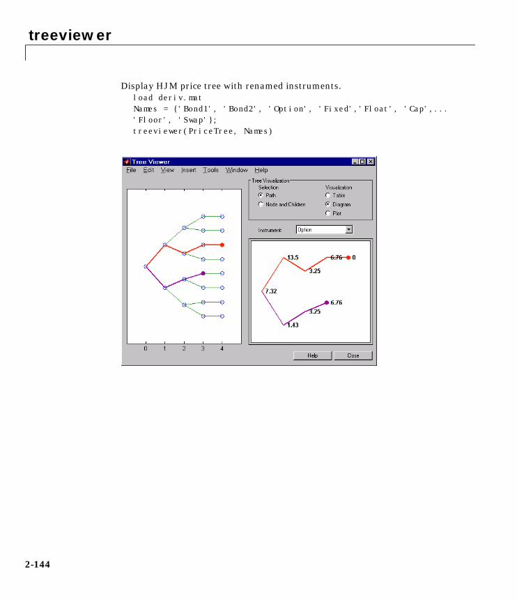
treeviewer
2-144
Display HJM price tree with renamed instruments.load deriv.matNames = {'Bond1', 'Bond2', 'Option', 'Fixed','Float', 'Cap',...'Floor', 'Swap'};treeviewer(PriceTree, Names)
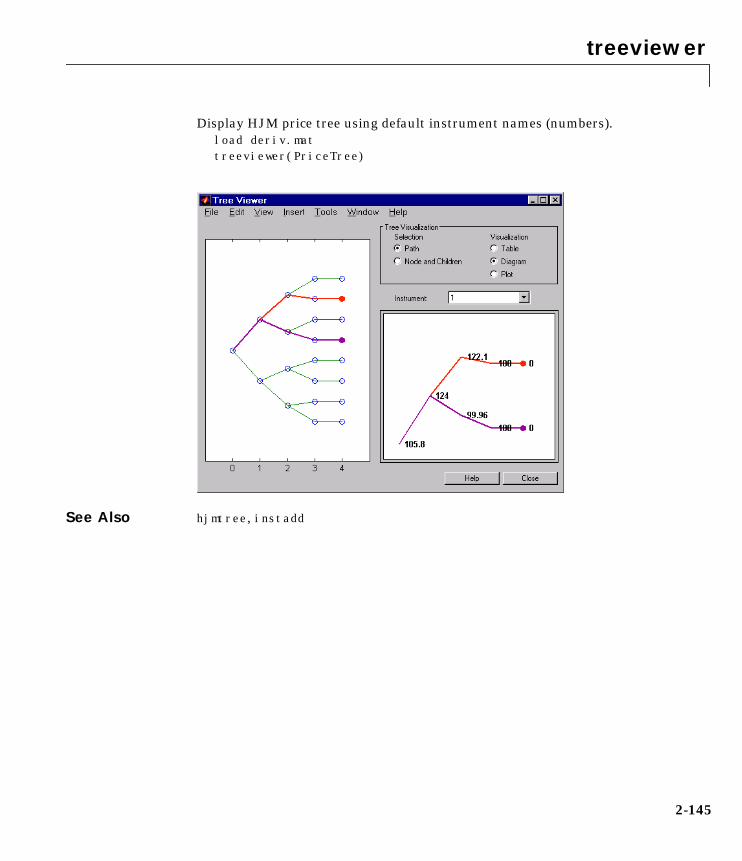
treeviewer
2-145
Display HJM price tree using default instrument names (numbers).load deriv.mattreeviewer(PriceTree)
See Also hjmtree, instadd

treeviewer
2-146

I-1
Index
Aarbitrary cash flow instruments 1-4
Bbond
defined 1-3bondbyhjm 2-9bondbyzero 2-12bushpath 2-15
example 1-44bushshape 2-16bushy tree 1-2
Ccap, defined 1-3capbyhjm 2-18cfbyhjm 2-20cfbyzero 2-21classfin 2-22constraints 1-82
dependent 1-82inconsistent 1-85
constructor 1-8convbyzero 2-24conventions in our documentation (table) vi
Ddate2time 2-24datedisp 2-26delta 1-33
defined 1-65dependent constraints 1-82derivgetbd 2-27derivsetbd 2-28
deterministic model 1-30disc2rate 2-30
purpose 1-16syntax 1-19
discount factors 1-16
Ffield 1-9fixed rate note, defined 1-3fixedbyhjm 2-32fixedbyzero 2-34floatbyhjm 2-36floatbyzero 2-38floating rate note, defined 1-3floor, defined 1-3floorbyhjm 2-40
Ggamma 1-33gamma, defined 1-65
HHeath-Jarrow-Morton (HJM) model 1-35Heath-Jarrow-Morton tree 1-48hedgeopt 2-42
purpose 1-64hedgeslf 2-45
purpose 1-64hedging
considerations 1-64functions 1-64goals 1-64
HJM pricing options structure 1-56

Index
I-2
hjmprice 1-48, 2-49hjmsens 2-51hjmtimespec 2-54HJMTree 1-48hjmtree 2-56
input arguments 1-35hjmvolspec 2-57
forms of volatility 1-36
Iinconsistent constraints 1-85instadd 2-59
creating an instrument 1-5instaddfield 2-61
creating new instruments 1-9instbond 2-65instcap 2-67instcf 2-69instdelete 2-71instdisp 2-73instfields 2-75instfind 2-78
purpose 1-11syntax 1-11
instfixed 2-81instfloat 2-83instfloor 2-85instget 2-87instgetcell 2-91instlength 2-96instoptbnd 2-97instrument index 1-11instselect 2-99
purpose 1-11instsetfield 2-102instswap 2-106
insttypes 2-108intenvget 2-110
purpose 1-27intenvprice 2-112intenvsens 2-114intenvset 2-116
purpose 1-25interest rate environment 1-16inverse discount 1-42isafin 2-120
Lleast squares problem 1-79
Mmkbush 2-121mmktbyhjm 2-122
Oobject 1-8optbndbyhjm 2-123Options 1-49
Pper-dollar sensitivities
calculating 1-62example 1-34
portfolio 1-5price tree structure 1-51Price vector 1-51pricing options structure 1-56

Index
I-3
Rrate specification 1-16rate2disc 2-127
creating inverse discounts 1-43purpose 1-16
RateSpec 1-36defined 1-16using 1-38
ratetimes 2-131purpose 1-16
recombining tree 1-2
Ssensitivities
per-dollar, example of 1-62stochastic model 1-30swap, defined 1-4swapbyhjm 2-135swapbyzero 2-138
TTimeSpec 1-36
using 1-39treeviewer 2-141
examining values with 1-52TypeString argument 1-5
Uunder-determined system 1-81
Vvanilla swaps 1-4vega, defined 1-65
VolSpec 1-36using 1-36

Index
I-4