Financial Crises, Bank Risk Exposureand

Government Financial Policy

Mark Gertler, Nobuhiro Kiyotaki, and Albert Queralto

N.Y.U. and Princeton

September 2010

Abstract

We develop a macroeconomic model with an intermediation sectorthat allow banks the option to issue outside equity as well as short termdebt. This makes bank risk exposure an endogenous choice. The goalis to have a model that can not only capture a crisis when financialinstitutions are highly vulnerable to risk, but can also account forwhy these institutions adopt such a risky portfolio structure in thefirst place. We use the model to assess quantitatively how perceptionsof fundamental risk and of government credit policy in a crisis ex postaffect the vulnerability of the financial system ex ante. We also studythe quantitative effects of macroprudential policies designed to offsetthe incentives for risk-taking.

1

1 Introduction

A distinguishing of the recent U.S. recesssion - known now as the GreatRecession - was the significant disruption of financial intermediation.1 Themeltdown of the shadow banking system along with the associated strainplaced on the commerical banking system led to an extraordinary increasein credit costs. This increase in credit costs, which peaked in the wakeof the Lehmann brothers collapse undoubtedly was a major factor in thecollapse of durable goods spending in the fall of 2008.that in turn triggeredthe extraordinary contraction in output and employment.The challenge for macroeconomists has been to build models that cannot

only capture this phenonomen but also be used to analyze the variety of un-conventional measures pursued by the Federal Reserve and the Treasury tostabilize credit markets. In this regard, there has been a rapidly growing lit-erature that attempts to incorporate financial factors within the quantitativemacroeconomic frameworks that had been the work horses for monetary andfiscal policy analysis up until this point.2 Much of this work is surveyed inGertler and Kiyotaki (2010). A common feature of these approaches has beento extend the basic financial accelerator mechanism developed by Bernankeand Gertler (1989) and Kiyotaki and Moore (1997) to banks in order tocapture the disruption of intermediation. Overall, this literature has madeprogress capturing in a broad brush way the basic real/financial interactionsover the crisis.Key to motivating a crisis within these frameworks is the heavy reliance

of banks on short term debt. This feature makes these institutions highlyexposed to the risk of adverse returns to their portfolio in way that is con-sistent with recent experience. Within these frameworks and most others inthis class, however, by assumption the only way banks can obtain externalfunds is by issuing short term debt.3 Thus, in their present form, these modelare not equipped to address how the financial system found itself so vulner-

1For descriptions, see Bernanke (2009) and Gorton (2010).2Examples of the work horse framework includes Christiano, Eichenbaum and Evans

(2005) and Smets and Wouters (2007).3Some quantitative macro models with financial sectors include: Bernanke, Gertler and

Gilchrist (1999), Brunnermeier and Sannikov (2009), Carlstrom and Fuerst (1997), Chris-tiano, Motto and Rostagno (2009), Mendoza (2010) and Jermann and Quadrini (2009).Only the latter consider both debt and equity finance, though they restrict attention toborrowing constraints faced by non-financial firms.

2

able in the first place. This question is of critical importance for designingpolicies to ensure the economy does not wind up in this position again. Forexample, as we discuss below, a number of authors have suggested that sucha risky bank liability structure was ultimately the product of expectationsthe government will intervene to stabilize financial markets in a crisis, justas it just did recently. With the existing macroeconomic frameworks it is notpossible to address this issue.In this paper we develop a macroeconomic model with an intermediation

sector that allow banks the option to issue outside equity as well as shortterm debt. This makes bank risk exposure an endogenous choice. Here thegoal is to have a model that can not only capture a crisis when financialinstitutions are highly vulnerable to risk, but also account for why these in-stitutions adopt such a risky portfolio structure in the first place. The basicframework builds on Gertler and Karadi (2010) and Gertler and Kiyotaki(2010). It extends the agency problem between banks and borrowers withinthese frameworks to allow intermediaries a meaningful tradeoff between shortterm debt and equity. Ultimately, a bank’s decision over its liability struc-ture depends on its perceptions of risk, which will in turn depend on thefundamental disturbances and expectations about government policy.We first use the model to analyze how different degrees of fundamental

risk in the economy affect the liability structure of banks and the overallmacroequilibrium. We then analyze the vulnerability of the economy to acrisis in each kind of risk enviroment. When perceptions of risk are low, banksopt for greater leverage. But this has the effect of making the economy morevulnerable to a crisis.We next turn to analyzing credit policy.during a crisis. Following Gertler

and Karadi (2010) and Gertler and Kiyotaki (2010), we analyze large scaleasset purchases of the type the Federal Reserve used to help stabilize financialmarkets following the Lehmann collapse. Within these frameworks, this kindof credit policy is effective in mitigating a crisis even if the central bank isless efficient in acquiring assets than is private sector. The advantage thecentral bank has during a crisis is that it can easily obtain funds by issuingshort term government debt, in contrast to private intermediaries that areconstrained by the weakness of their respective balance sheets.What is new in the present framework is that it is possible to capture

costs of the credit market policy associated with moral hazard. In partic-ular, as we show, the anticipated credit policy will induce banks to adopta riskier liability structure, which will in turn require a larger scale credit

3

market interevention during a crisis. This sets the stage for an analysis ofmacroprudential policy designed to offset the effects of credit policy on theincentives for bank risk-taking.To be sure, there is lengthy theoretical literature that examines the

sources of vulnerability of a financial system. For example, Fostel andGeanokoplos (2009) stress the role of investor optimism.in encouraging risktaking. Others such as Diamond and Rajan (2009), Fahri and Tirole (2009)and Chari and Kehoe (2009) stress moral hazard consequences of bailouts andother credit market interventions. Our paper differences mainly by couch-ing the analysis within a full blown macroeconomic model to provide a steptoward assessing the quantitative implications.There is as well a related literature that analyzes macroprudential policy.

Again, much of it is qualitative (e.g. Lorenzoni, 2009, Korinek, 2009, andStein 2010). However, there are also quantitative frameworks, e,g, Bianchi(2009) and Nikolov (2010). Our framework differs by exploring the inter-action between credit policies used to stabilize the economy ex post andmacroprudential policy used to mitigate risk taking ex ante. In addition, weendogenize the financial market friction.Finally relevant are the literatures on international risk sharing and on

asset pricing and business cycles.4 Conventional quantitative models usedfor policy evaluation typically examine linear dynamics within a local neigh-borhood of a deterministic steady state. In doing so they abstract from anexplicit consideration of uncertainty. Because bank liability structure willdepend on perceptions of risk, however, accounting for uncertainty is crit-ical. Here we borrow insights from these literatures by considering secondorder approximations to pin down determinate bank liability shares.Section 2 develops the model. Section 3 uses the model to analyze crises

and policy. Concluding remarks are in sections 4.

2 The Baseline Model

As we noted, our approach to incorporating financial frictions within a busi-ness cycle model is a variation of Gertler and Kiyotaki (2010) and Gertler

4See, for example, Devereux and Sutherland (2009) and Tille and Van Wincoop (2007)for examples of the former and Campbell (1993) and Lettau (2003) for examples of thelatter.

4

and Karadi (2010).5 As in these frameworks financial intermediaries faceendogenous balance sheet constraints because of the moral hazard problemdescribed shortly. One important difference is that we allow intermediariesto issue state-contingent debt (outside equity) as well as non-contingent shortterm debt. This gives intermediaries more meaningful flexibility over theirrisk exposure. We can then use the model to analyze how perceptions of assetreturn risk as well as government policy interventions influence the degree ofrisk exposure that intermediaries choose. This in turn sets the stage for ananalysis of macro-prudential policies.As in our earlier work we keep the core model simple enough to see clearly

the role of financial intermediation, but rich enough to allow for rough quan-titative analysis. As in Gertler and Kiyotaki (2010), we restrict attention toa purely real model but abstract from bank liquidity risk, which was a centralfeature of that analysis. Adding this consideration back in is straightforward,as would be including nominal rigidities and money, following Gertler andKaradi (2010).6

We begin with the basic physical environment and then turn to the be-havior of households, intermediaries and nonfinancial firms.

2.1 Physical Setup

Before introducing financial frictions, we present the basic physical environ-ment.There are a continuum of firms of mass of unity. Each firm produces

output using an identical constant returns to scale Cobb-Douglas productionfunction with capital and labor as inputs. We can express aggregate outputYt as a function of aggregate capital Kt and aggregate labor hours Lt as:

Yt = AtKtαL1−αt , 0 < α < 1, (1)

5Some other recent monetary DSGE models that incorporate financial factors includeChristiano, Motto, and Rostagno (2009) and Gilchrist, Ortiz and Zakresjek (2009).

6Much of the insight into how credit market frictions may affect real activity and howvarious credit policies may work can be obtained from studying a purely real model. Thereare, however, several insights that monetary models add, however. First, if the zero lowerbound on the nominal interest is binding, the financial market disruptions will have a largereffect than otherwise. This is because the central bank is not free to further reduce thenominal rate to offset the crisis. Second, to the extent there are nominal price and/or wagerigidities that induce countercyclical markups, the effect of the credit market disruptionand aggregate activity is amplified. See, e.g., Gertler and Karadi (2010) and Del Negro,Ferrero, Eggertsson and Kiyotaki (2010) for an illustration of both of these points.

5

whereAt is aggregate productivity, which follows a stationaryMarkov process.Let Kt be the aggregate capital stock at t and St denote the aggregate

capital stock "in process" for period t+ 1 . Capital in process at t for t+ 1is the sum of current investment It and the stock of undepreciated capital,(1− δ)Kt.

St = (1− δ)Kt + It. (2)

Capital in process for period t, St−1 is transformed into capital after therealization of a multiplicative shock to capital quality, ψt.

Kt = ψtSt−1 (3)

Following the finance literature (e.g., Merton (1973)), we introduce the cap-ital quality shock as a simple way to introduce an exogenous source of vari-ation in the value of capital. As will become clear later, the market price ofcapital will be endogenous within our framework. In this regard, the capitalquality shock will serve as an exogenous trigger of asset price dynamics. Therandom variable ψt+1 is best thought of as capturing some form of economicobsolescence, as opposed to physical depreciation.7 We assume the capi-tal quality shock ψt+1 also follows a Markov process, with an unconditionalmean of unity. In addition, we allow for occasional disasters in the form ofsharp contractions in quality, as describe later. These disaster shocks serveto instigate financial crises.8

Firms acquire new capital from capital goods producers. There are convexadjustment costs in the gross rate of change in investment for capital goodsproducers. Aggregate output is divided between household consumption Ct,investment expenditures, and government consumption Gt,

Yt = Ct + [1 + f(ItIt−1

)]It +Gt (4)

7One way to motivate this disturbance is to assume that final output is a C.E.S. com-posite of a continuum of intermediate goods that are in turn produced by employingcapital and labor in a Cobb-Douglas production technology. Suppose that, once capital isinstalled, capital is good-specific and that each period a random fraction of goods becomeobsolete and are replaced by new goods. The capital used to produced the obsolete goodsis now worthless and the capital for the new goods is not fully on line. The aggregatecapital stock will then evolve according to equation. (3).

8Other recent papers that make use of this kind of disturbance include, Gertler andKaradi (2010), Brunnermeier and Sannikov (2009) and Gourio (2009). An alternative(but more cumbersome) approach would be to introduce a "news" shock that affectscurrent asset values. Gertler and Karadi (2010) illustrate the similarities between the twoapproaches.

6

where f( ItIt−1)It reflects physical adjustment costs, with f(1) = f 0(1) = 0 and

f 00(It/It−1) > 0. Thus the aggregate production function of capital goodsproducers is decreasing returns to scale in the short-run and is constantreturns to scale in the long-run.Next we turn to preferences. Our exact specification follows Miao and

Wang (2010), which is in turn based on Guvenen (2009) and Greenwood,Hercowitz and Huffman (GHH, 1988):

Et

∞Xτ=t

βτ−t1

1− γ

µCτ − hCτ−1 −

χ

1 + ϕL1+ϕτ

¶1−γ(5)

where Et is the expectation operator conditional on date t information andγ > 0. The preference specification allows for both habit formation and GHHpreferences over hours: The latter, of course, eliminates wealth effects fromlabor supply. As will become clear, these features improve the ability for themodel to capture business cycle dynamics despite the absence of labor marketfrictions. At the same time, they permit introducing reasonable degrees ofrisk aversion to examine asset pricing and portfolio structure.We abstract from many frictions in the conventional DSGE framework

(e.g. nominal price and wage rigidities, variable capital utilization, etc.).9

However, we allow both habit formation of consumption and adjustmentcosts of investment because, as the DSGE literature has found, these featuresare helpful for reasonable quantitative performance and because they can bekept in the model at minimal cost of additional complexity.If there were no financial frictions, the competitive equilibrium would

correspond to a solution of the planner’s problem that involves choosingaggregate quantities (Yt, Lt, Ct, It, St) as a function of the aggregate state(Ct−1, It−1, St−1, At, ψt) in order to maximize the expected discounted utilityof the representative household subject to the resource constraints. Thisfrictionless economy will serve as a benchmark to which we may compare theimplications of the financial frictions.In what follows we will introduce banks that intermediate funds between

households and nonfinancial firms. We will also introduce financial frictionsthat may impede credit flows. A new feature of the model is that banks canoffer households state-contingent liabilities as well as non-contingent liabili-ties. We will then study the consequences for real activity and also analyzethe implications for government policy.

9See, e.g.,Christiano, Eichenbaum and Evans (2005) and Smets and Wouters (2007).

7

2.2 Households

In our economy with credit frictions, households lend to nonfinancial firmsvia financial intermediaries. Following Gertler and Karadi (2009) and Gertlerand Kiyotaki (2010), we formulate the household sector in way that permitsmaintaining the tractability of the representative agent approach.In particular, there is a representative household with a continuum of

members of measure unity. Within the household there are 1 − f "work-ers" and f "bankers". Workers supply labor and return their wages to thehousehold. Each banker manages a financial intermediary (which we will calla "bank") and transfers nonnegative dividends back to household subject toits flow of fund constraint. Within the family there is perfect consumptioninsurance.Households do not acquire capital nor do they provide funds directly to

nonfinancial firms. Rather, they supply funds to banks. (It may be best tothink of them as providing funds to banks other than the ones they own).Banks offer two types of liabilities to households: non-contingent risklessshort term debt (deposits) and equity, which may be thought of as perfectlystate contingent debt. We refer to equity issued by banks and held by house-holds as "outside" equity. This contrasts with the accumulated retainedearnings of a banker who manages an intermediary and is involved in theoperation. We refer to the latter as "inside" equity. The distinction betweenoutside and inside equity will become important later since banks will faceconstraints in obtaining external funds.In addition, households may acquire short term riskless government debt.

Both intermediary deposits and government debt are one period real bondsthat pay the gross real return Rt from t − 1 to t. In the equilibrium weconsider, the instruments are both riskless and are thus perfect substitutes.Thus, we impose this condition from the outset. As will be clear later, it willnot matter in our model whether households hold government debt directlyor do so indirectly via financial intermediaries (who in turn issue deposits tohouseholds.)We normalize the units of outside equity so that each equity is a claim to

the future returns of one unit of the asset that the bank holds. Let Zt be theflow returns at t generated by one unit of the bank’s assets and qt the priceof the outside equity at t. Then the payoff at t for a share of outside equityacquired at t− 1 equals [Zt + (1− δ)qt]ψt. Note that the payoff is adjustedfor both the physical depreciation and the quality adjustment of the capital

8

that underlies bank assets.The household chooses consumption, labor supply, riskless debt, and out-

side equity (Ct, Lt,Dht, et) to maximize expected discounted utility (5) sub-ject to the flow of funds constraint,

Ct +Dht + qtet =WtLt +Πt − Tt +RtDht−1 + [Zt + (1− δ)qt]ψtet−1. (6)

Here Wt is the wage rate, Tt is lump sum taxes, and Πt is net distributionsfrom ownership of both banks and nonfinancial firms. Let uCt denote themarginal utility of consumption andΛt,t+1 the household’s stochastic discountfactor. Then the household’s first order conditions for labor supply andconsumption/saving are given by

EtuCt

(Ct − hCt−1 − χ1+ϕ

L1+ϕt )−γWt = χLϕ

t , (7)

Et (Λt,t+1)Rt+1 = 1, (8)

Et(Λt,t+1Ret+1) = 1 (9)

with

uCt ≡ (Ct − hCt−1 −χ

1 + ϕL1+ϕt )−γ − βh(Ct+1 − hCt

χ

1 + ϕL1+ϕt+1 )

−γ

Λt,τ ≡ βτ−tuCτuCt

.

Ret+1 =[Zt+1 + (1− δ)qt+1]ψt+1

qt

Because banks may be financially constrained, bankers will retain earn-ings to accumulate assets. Absent some motive for paying dividends, theymay find it optimal to accumulate to the point where the financial constraintthey face is no longer binding. In order to limit bankers’ ability to save toovercome financial constraints, we allow for turnover between bankers andworkers. In particular, we assume that with i.i.d. probability 1−σ, a bankerexits next period, (which gives an average survival time = 1

1−σ ). Upon ex-iting, a banker transfers retained earnings to the household and becomesa worker. Note that the expected survival time may be quite long (in our

9

baseline calibration it is eight years.) It is critical, however, that the expectedhorizon is finite, in order to motivate payouts while the financial constraintsare still binding.Each period, (1 − σ)f workers randomly become bankers, keeping the

number in each occupation constant. Finally, because in equilibrium bankerswill not be able to operate without any financial resources, each new bankerreceives a "start up" transfer from the family as a small constant fraction ofthe total assets of entrepreneurs. Accordingly, Πt is net funds transferred tothe household, i.e., funds transferred from exiting bankers minus the fundstransferred to new bankers (aside from small profits of capital goods produc-ers).An alternative to our approach of having a consolidated family of work-

ers and bankers would be to have the two groups as distinct sets of agents,without any consumption insurance between the two groups. It is unlikely,however, that the key results of our paper would change qualitatively. Bysticking with complete consumption insurance, we are able to have lendingand borrowing in equilibrium and still maintain the tractability of the rep-resentative household approach.

2.3 Nonfinancial Firms

There are two types of nonfinancial firms: goods producers and capital pro-ducers.

2.3.1 Goods Producers

Competitive goods producers operate a constant returns to scale technologywith capital and labor inputs, given by equation (1). Firms choose labor tosatisfy

Wt = (1− α)YtLt

(10)

It follows that we may express gross profits per unit of capital Zt as follows:

Zt =Yt −WtLt

Kt= αAt

µLt

Kt

¶1−α. (11)

A goods producer does not face any financial frictions in obtaining fundsfrom banks and can commit to pay all the future gross profits to the creditor

10

bank. In particular, we suppose that the bank is efficient at evaluating andmonitoring nonfinancial firms and also at enforcing contractual obligationswith these borrowers. That is why these borrowers rely exclusively on banksto obtain funds. A goods producer with an opportunity to invest obtainsfunds from a bank by issuing new state-contingent securities at the price Qt.The producer then uses the funds to buy new capital goods from capitalgoods producers. Each unit of the security is a state-contingent claim to thefuture returns from one unit of investment:

ψt+1Zt+1, (1− δ)ψt+1ψt+2Zt+2, (1− δ)2ψt+1ψt+2ψt+3Zt+3, ... .

Through perfect competition, the price of new capital goods is equal to Qt,and goods producers earn zero profits state-by-state.

2.3.2 Capital Goods Producers

Capital producers make new capital using input of final output and subject toadjustment costs, as described in section 2.2. They sell new capital to firmsat the price Qt. Given that households own capital producers, the objectiveof a capital producer is to choose It to solve:

maxEt

∞Xτ=t

Λt,τ

½QτIτ −

∙1 + f

µIτIτ−1

¶¸Iτ

¾From profit maximization, the price of capital goods is equal to the marginalcost of investment goods production as follows,

Qt = 1 + f

µItIt−1

¶+

ItIt−1

f 0(ItIt−1

)−EtΛt,t+1(It+1It)2f 0(

It+1It) (12)

Profits (which arise only outside of steady state), are redistributed lump sumto households.

2.4 Banks

To provide funds to goods producers in each period, banks raise funds bothinternally from retained earnings and externally from households. At thebeginning of the period each bank raises deposits dt and outside equity etfrom households. In addition the bank has its own net worth, nt accumulated

11

from retained earnings. We refer to nt as inside equity. The bank then usesall its available funds to make loans to nonfinancial firms.Financial frictions affect real activity in our framework via the impact on

funds available to banks. As noted earlier, however, there is no friction intransferring funds between a bank and nonfinancial firms: Given its supplyof available funds, a bank can lend frictionlessly to nonfinancial firms againsttheir future profits. In this regard, firms are able to offer banks a perfectlystate-contingent security.Along with raising funds via deposits and outside equity issues from

households, a bank decides the volume of loans st to make to nonfinancialfirms. Qt is the price of a state-contingent security (or "asset") - i.e. themarket price of the bank’s claim on the future returns from one unit of anonfinancial firm’s capital at the end of period t (i.e. capital at t in processfor t+ 1).For an individual bank, the flow-of-funds constraint implies the value of

loans funded within a given period, Qtst, must equal the sum of bank networth nt, and funds raised from households, consisting of outside equity qtetand deposits dt.

Qtst = nt + qtet + dt. (13)

Note that in general, Qt need not equal qt. As will become clear, when thebank is financially constrained, the price of outside equity, qt, will in generalexceed the value of a bank’s claim on a unit of capital of nonfinancial firm,Qt, given that only banks can provide funds costlessly to goods producers.While banks may issue new outside equity, they raise inside equity only

through retained earnings.10 Since inside equity involves management andcontrol of the firm’s assets, we suppose it is prohibitively costly for the ex-isting insiders to bring in new ones with sufficient wealth. In particular, thebank’s net worth nt at t is the gross payoff from assets funded at t− 1, netof returns to outside equity holders and depositors, as follows:

nt = [Zt + (1− δ)Qt]ψtst−1 − [Zt + (1− δ)qt]ψtet−1 −Rtdt−1 (14)

where, as before, Zt is the dividend payment at t on the loans the bankfunds at t− 1. Observe that outside equity permits the bank to hedge risks10As a crude first pass, it might be useful to think of inside equity as common equity

and outside equity as preferred equity. Insiders in a firm are more likely to hold the formerand outsiders the latter. This is because common equity holders are the firm’s ultimateresidual claimants, while preferred equity holders receive a smoother stream of returns. Ingeneral, common equity is thought to be more costly to issue than preferred equity.

12

associated with shocks to both Zt and the asset quality shock ψt. It is thishedging value that makes it attractive to the bank to issue outside equity.When the bank is financial constrained, it finds it optimal to accumulate

retained earnings until the time it exits. Accordingly, given that the bankpays dividends only when it exits (which occurs with a constant probability),the objective of the bank at the end of period t is the expected present valueof future terminal dividend payout, as follows

Vt = Et

" ∞Xτ=t+1

(1− σ)στ−t−1Λt,τnτ

#(15)

To motivate an endogenous constraint on the bank’s ability to obtainfunds, we introduce the following simple agency problem: We assume thatafter a bank obtains funds, the banker managing the bank may transfer afraction of assets to his or her family. It is the recognition of this possibilitythat has households limit the funds they lend to banks.In addition, we assume that the fraction of funds the bank may divert,

further, depends on the composition of its liabilities. In particular, we as-sume that at the margin it is more difficult to divert assets funded by shortterm deposits than by outside equity. Short term deposits require the bankto continuously meet a non-contingent payment. Dividend payments, in con-trast, are tied to the performance of the bank’s assets, which is difficult foroutsiders to monitor. By giving banks less discretion over payouts, short termdeposits offer more discipline over bank managers than outside equity.11

Let xt denote the fraction of bank assets funded by outside equity, asfollows:

xt =qtetQtst

(16)

Then we assume that after the bank has obtained funds it may divert thefraction Θ(xt) of assets, where Θ(xt) is the following convex function of xt:

Θ(xt) = θ³1 + εxt +

κ

2x2t

´(17)

We allow for the possibility that there could be some efficiency gains inmonitoring the bank from having at least a bit of outside equity participationin funding the bank (i.e. ε can be negative). However, we restrict attention to

11The idea that short term debt serves as a disciplining devices over banks is due toCalomiris and Kahn (1991).

13

calibrations where the bank’s ability to divert assets increases when outsideequity replaces deposits for funding at the margin, i.e., θ(ε+κxt) is positive.Finally, we assume that the banker’s decision over whether to divert fundsmust be made at the end of the period t but before the realization of aggregateuncertainty in the following period. Here the idea is that if the banker isgoing to divert funds, it takes time to position assets and this must be donebetween the periods (e.g., during the night).If a bank diverts assets for its personal gain, it defaults on its debt and is

shut down. The creditors may re-claim the remaining fraction 1− Θ(xt) offunds. Because its creditors recognize the bank’s incentive to divert funds,they will restrict the amount they lend. In this way a borrowing constraintmay arise.Let Vt(st, et, dt) be the maximized value of the bank’s objective Vt, given

an asset and liability configuration (st, et, dt) at the end of period t. Thenin order to ensure the bank does not divert funds, the following incentiveconstraint must hold:

Vt ≥ Θ(xt)Qtst, (18)

Equation (18) states simply that for households to be willing to supply fundsto a bank, the bank’s franchise value Vt must be at least as large as its gainfrom diverting funds.In general the franchise value of the bank at the end of period t−1 satisfies

the Bellman equation

Vt−1(st−1, et−1, dt−1) (19)

= Et−1Λt−1,t(1− σ)nt + σMaxst,et.dt

[Vt(st, et, dt)]. (20)

where the right side takes into account that the bank exits with probability1− σ and continues with probability σ.To solve the decision problem, we first guess that the value function is

linear in the bank portfolio structure as follows:

Vt(st, et, dt) = νstst − νetet − νtdt (21)

where νst is the shadow value to the bank of a unit of assets, νet is the shadowcost of a unit of outside equity and νt is the shadow cost of a unit deposits.Next, let μst be the excess value of a unit of bank assets over deposits and

14

μet the excess value per unit from switching from deposits to outside equityfinance, as follows:

μst ≡νstQt− νt, (22)

μet ≡ νt −νetqt.

Then combining the flow of funds constraint (13) with equation (21) allows usto write the conjectured solution for Vt in terms of excess values, as follows:

Vt(st, et, dt) = μstQtst + μetqtet + νtnt (23)

Now insert the conjectured solution (23) for Vt(st, et, dt) into the Bellmanequation (19) and use the relation xt = qtet/Qtst to eliminate et. Then maxi-mize this objective with respect to the to the incentive constraint (18). Giventhat λt is the Lagrangian multiplier with respect to the incentive constraint,the first order necessary conditions for xt, st and λt yield:

(1 + λt)μet = λtθ(ε+ κxt), (24)

(1 + λt) (μst + xtμet) = λtθ³1 + εxt +

κ

2x2t

´, (25)

[μst + xtμet]Qtst + νtnt = Θ(xt)Qtst. (26)

The left side of equation (24) is the marginal benefit to the bank from sub-stituting outside equity finance for unit of short term debt. The right sideis the marginal cost, equal to the increase in the fraction of assets the bankcan divert times the shadow value of the incentive constraint λt.The first order condition for Equation (25) implies that the marginal

benefit from increasing asset st adjusted for additional equity finance, μst +xtμet is equal to the marginal cost of tightening the incentive constraint byθ¡1 + εxt +

κ2x2t¢.

Finally, the first order condition for λt yields the incentive constraint.From (25), we learn that the incentive constraint binds (λ is positive) onlyif the adjusted excess value of bank assets μst + xtμet is positive.Combing equations (24, 25) yields a relation for xt the is increasing in the

ratio of excess values μet/μst :

15

xt = −(μetμst)−1 +

s(μetμst)−2 +

2

κ(1− ε(

μetμst)−1) (27)

≡ x

µμetμst

¶, where x0 > 0 given κ >

1

2ε2.

Next, let φt be the maximum ratio of bank assets to net worth to satisfiesthe incentive constraint. Then rearranging the incentive constraint yields thefollowing relation between Qtst and nt.

Qtst = φtnt (28)

withφt =

νtΘ(xt)− (μst + xtμet)

. (29)

Equation (28) is a key relation of the banking sector: It indicates thatwhen the borrowing constraint binds, the total quantity of private assetsthat a bank can intermediate is limited by its internal equity, nt.The relationis fairly intuitive: φt is increasing in the adjusted excess value of banksassets (μst + xtμet) and the opportunity cost of a unit net worth νt (whichcorresponds to the shadow cost of a unit of deposits). Both these factorsraise the franchise value of bank in (23), which reduces the banks incentiveto divert funds. This makes creditors willing to fund more assets for a givenlevel of bank net worth. Conversely, φt is decreasing in Θ(xt), the fraction offunds banks are able to divert.Next, insert the conjectured value function back into the Bellman to solve

for the undetermined coefficients. Then the solutions for the undeterminedcoefficients (νt, μst, μet) are given by,

νt = Et(Λt,t+1Ωt+1)Rt+1, (30)

μst = Et[Λt,t+1Ωt+1(Rkt+1 −Rt+1)] (31)

μet = Et[Λt,t+1Ωt+1(Rt+1 −Ret+1)] (32)

withΩt+1 = 1− σ + σ[νt+1 + φt+1(μst+1 + xt+1μet+1)] (33)

Rkt+1 =[Zt+1 + (1− δ)Qt+1]ψt+1

Qt(34)

16

and where the return on outside equity Ret+1 is given by equation (9). Ωt+1

denotes the shadow value of a unit of net worth to the bank and Rkt+1 is therate of return on asset held from t to t+ 1.Note first that the shadow value of net worth for next period, Ωt+1 is

the probability weighted average of the marginal values for exiting and forcontinuing banks. For an exiting bank, the marginal value is unity - i.e.,equivalent to an additional unit of consumption goods. For a continuing bankit is the sum of the saving on deposits νt+1 and the payoff from being ableto hold more assets: the product of the leverage ratio φt+1 and the adjustedexcess value μst+xtμet. Since both the leverage ratio and excess returns varycountercyclically, so too will the shadow value of net worth. Put differently,because the bank’s incentive constraint is tighter in recessions than in booms,an additional unit of net worth is more valuable in bad times than in goodtimes.Let us define the "augmented stochastic discount factor" as the house-

hold stochastic discount factor Λt,t+1 multiplied by the stochastic marginalvalue of net worth Ωt+1. Since both Ωt+1 and Λt,t+1 are counter-cyclical, theaugmented stochastic discount factor is more volatile than the household sto-chastic discount factor. According to (30), the cost of deposits per unit tothe bank νt is the expected product of the augmented stochastic discountfactor and the deposit rate Rt+1.From (31), the excess value of assets per unit, μst, is the expected value

of the product of the augmented stochastic discount factor and the excessreturn Rkt+1−Rt+1. Note that since the excess return to assets Rkt+1−Rt+1

tends to be procyclical while Ωt+1 is counter-cyclical, the volatility in theshadow value of net worth has the effect of reducing the continuation valueof the bank, and thus the leverage ratio φt. In this way, uncertainty affectsthe bank’s ability to obtain funds.From (32), the excess value of outside equity issue is the expected value

of the product of the augmented stochastic discount factor and the differencein the rate of returns on deposit and outside equity Rt+1 −Ret+1. From thehousehold’s portfolio decision, we learn the arbitrage relation between thedeposit rate and the return on outside equity:

Et[Λt,t+1(Rt+1 −Ret+1)] = 0 (35)

Observe that the household discounts the returns by the stochastic factorΛt,t+1 while the banker uses a discount factor Λt,t+1Ωt+1, which fluctuates

17

more counter-cyclically. As a consequence, the bank obtains hedging valueby switching from deposits to outside equity: The excess value of outsideequity issue μet = Et[Λt,t+1Ωt+1(Rt+1 −Ret+1)] is positive.Absent any cost of issuing state-contingent liabilities, the bank would

move to one hundred percent outside equity finance. However, increasingthe fraction of outside equity enhances the incentive problem by makingit easier for bankers to divert funds, as equation (18) suggests. Thus thebank faces a trade-off in issuing outside equity. In general, there will be aninterior solution for outside equity finance. Later we explore whether or notthe decentralized solution is socially optimal.While outside equity improves banks’ ability to hedge fluctuations in net

worth, what matters for the overall outside credit they can obtain is theirinternal equity, or net worth, along with the maximum feasible leverage ratioφt. Since φt does not depend on bank-specific factors, we can aggregate equa-tion (28) to obtain a relation between the aggregate demand for securitiesby banks Spt and aggregate net worth in the banking sector Nt.

QtSpt = φtNt (36)

The evolution of Nt accordingly plays an important role in the dynamics ofthe model economy. We turn to this issue next.

2.5 Evolution of Aggregate Bank Net Worth

Total net worth in the banking sector banks, Nt, equal the sum of the networth of existing entrepreneurs Not (o for old) and of entering entrepreneursNyt (y for young):

Nt = Not +Nyt. (37)

Net worth of existing entrepreneurs equals earnings on assets held in theprevious period net the cost of outside equity finance and the cost of depositfinance, multiplied by the fraction that survive until the current period, σ:

Not = σ[Zt + (1− δ)Qt]ψtSt−1 − [Zt + (1− δ)qt]ψtet−1 −RtDt−1. (38)

Since new bankers cannot operate without any net worth, we assume thatthe family transfers to each one the fraction ξ/(1−σ) of the total value assetsof exiting entrepreneurs, where ξ is a small number. This implies:

Nyt = ξ[Zt + (1− δ)Qt]ψtSt−1. (39)

18

In the calibration that follows, we choose ξ so that in steady state, the ratioof bank assets to net worth is approximately equal to the observation inthe US. Note that the functional form of the transfer is chosen for technicalconvenience.

Nt = (σ + ξ) [Zt + (1− δ)Qt]ψtSt−1 − σ [Zt + (1− δ)qt]ψtet−1 − σRtDt−1(40)

Observe that the evolution of net worth depends on fluctuations in thereturn to assets. Further, the higher the leverage of the bank is, the largerwill be the percentage impact of return fluctuations on net worth. The useof outside equity, however, reduces the impact of return fluctuations on networth.Note finally that a deterioration of capital quality (a decline in ψt) directly

reduces net worth. As we will show, there will also be a second round effect,as the decline in net worth induces a fire sale of assets, depressing asset pricesand thus further depressing bank net worth.12

2.6 Credit Policy

Earlier we characterized how the total value of privately intermediated as-sets, QtSpt, is determined. We now suppose that the central bank is willingto facilitate lending. As we discussed earlier, this kind of credit policy cor-responds to the central bank’s large scale purchase of high grade privatesecurities, which was at the center of its attempt to stabilize credit marketsduring the peak of the financial crisis.13 Let QtSgt be the value of assetsintermediated via government assistance and let QtSt be the total value ofintermediated assets: i.e.,

12According to the profit distribution, the net profit transfer from banks and capitalgoods producers to the representative household is

Πt = QtIt − It

∙1 + f

µItIt−1

¶¸− ξ[Zt + (1− δ)Qt]ψtSt−1

+(1− σ) [Zt + (1− δ)Qt]ψtSt−1 − [Zt + (1− δ)qt]ψtet−1 −RtDt−1 .

13Accordingly, this analysis concentrates on the central bank’s direct lending programswhich we think were the most important dimension of its balance sheet activities. SeeGertler and Kiyotaki (2010) for a formal characterization of the different types of creditmarket interventions that the Federal Reserve and Treasury pursued in the current crisis.

19

QtSt = QtSpt +QtSgt (41)

To conduct credit policy, the central bank issues government debt tohouseholds that pays the riskless rate Rt+1 and then lends the funds to non-financial firms at the market lending rate Rkt+1.We suppose that governmentintermediation involves efficiency costs: in particular, the central bank creditinvolves an efficiency cost of τ per unit supplied. This deadweight loss couldreflect the administrative costs of raising funds via government debt. It mightalso reflect costs to the central bank of identifying preferred private sector in-vestments. On the other hand, the government always honors its debt: thus,unlike the case with private financial institutions there is no agency conflictthan inhibits the government from obtaining funds from households. Put dif-ferently, unlike private financial intermediation, government intermediationis not balance sheet constrained.14

Accordingly, suppose the central bank is willing to fund the fraction ζt ofintermediated assets: i.e.,

Sgt = ζtSt (42)

As we show, by increasing ζt the central bank can reduce the excess returnμst = Et[Λt,t+1Ωt+1(Rkt+1 −Rt+1)]. In this way credit policy can reduce thecost of capital, thus stimulating investing. Later we describe how the centralbank may choose the path of ζt to combat a financial crisis.Finally, to fund its asset purchases the central bank can issue government

debt Dgt equal to ζtQtSt. Its net earnings from intermediation in any periodt thus equals (Rkt+1 − Rt+1)Dgt. These net earnings provide a source ofgovernment revenue and must be accounted for in the budget constraint, aswe discuss next.14An equivalent formulation of credit policy has the central bank issue government debt

to financial intermediaries. Intermediaries in turn fund their government debt holdings byissuing deposits to households that are perfect substitutes. Assuming the agency problemapplies only to the private assets it holds, a financial intermediary is not constrained infinancing its government debt holdings. Thus, only the funding of private assets by finan-cial institutions is balance sheet constrained. As in the baseline scenario, the central bankis able to elastically issue government debt to fund private assets. It is straightforward toshow that the equilibrium conditions in the scenario are identical to those in the baselinecase. (The identical intermediary balance sheet constraint on private assets holds). Onevirture of this scenario is that the intermediary holdings of government debt are inter-pretable as interest bearing reserves, which is how the central bank has funded its assetsin practice.

20

2.7 Government Budget Constraint

Government expenditures consist of government consumption G, which wehold fixed, and monitoring costs from central bank intermediation:

Gt = G+ τSgt, (43)

The government budget constraint, in turn is

Gt +QtSgt +RtDgt−1 = Tt + [Zt + (1− δ)Qt]ψtSgt−1 +Dgt, (44)

where Tt is lump-sum taxes on the household.

2.8 Equilibrium

To close the model, we require market clearing in both the market for banksecurities St, outside equity, et, and deposits Dt.Market clearing for bank securities requires that the total supply of secu-

rities given by equation (2) net government security purchases, must equalprivate demand Spt given by equations (36) and (29). This implies,

Qt(St − Sgt) =νt

θ(1 + εxt + x2t )− (μst + xtμet)Nt, (45)

Similarly in the market equilibrium for outside equity, the demand by house-holds et equals the supply by banks et

qtet = xt ·QtSt, (46)

where the fraction of total assets funded by outside equity xt is given by equa-tion (27). Finally, given the flow of funds constraint, equilibrium depositsmust equal aggregate bank assets net outside equity and net worth:

Dt = Dht −Dgt = (1− xt)QtSt −Nt. (47)

The final equilibrium condition is that labor demand equals labor supply,which requires

(1− α)YtLt·Et

"uCt

(Ct − hCt−1 − χ1+ϕ

L1+ϕt )−γ

#= χLϕ

t (48)

21

To close the model we need to describe the exogenous processes for theproductivity shock At and the capital quality shock ψt. Since we wish toconcentrate on the impact of the capital quality shock, we simply fix At to aconstant value A,

At = A (49)

The capital quality shock, in contrast, follows a AR(1) process that allowsfor the possibility of infrequent "disasters". In particular: ψt is the product ofa process that evolves in normal times, eψt, and one that arises in "disasters"eψD

t

ψt = eψteψD

t

with

log eψt = ρ0ψ + ρψ log eψt−1 + σ ψt (50)

log eψD

t = ρψ log eψD

t−1 + ηt (51)

where ψt is distributed N(0, 1), and ηt is distributed binomial:

ηt =

½−∆+ π∆ with prob. ππ∆ with prob 1− π

¾where ∆ is a positive number, implying the disaster innovation −∆ is nega-tive. We normalize the process so that the mean of ηt is zero and the varianceis:

E(η2t ) = π(1− π)∆2; (52)

In practice, assuming the disaster shock ∆ is not too large, we will beable to capture risk with a second order approximation of the model. In thisinstance, what will matter for capturing risk is the overall standard deviationof the combined ψt shock. We introduce the disaster formulation to enrichthe economic interpretation of the model.The equations (1, 2, 3, 4, 6, 8, 9, 11, 12, 27, 30, 31, 32, 40, 45, 46, 47, 48) de-

termine the seventeen endogenous variables (Yt, Kt, St, Ct, It, Lt, Zt, Rt+1, qt,νt,μst, μet, xt, Qt, Nt, et, Dt) as a function of the state variables (St−1, Ct−1, It−1,et−1, RtDt−1, RtDgt−1, Sgt−1, At, ψt), together with the exogenous stochastic

22

process of (At, ψt) and the government policy vector of (Gt, Tt, Sgt, Dgt). Oneof these eighteen equations is not independent by Walras Law.Absent credit market frictions, the model reduces to a real business cycle

framework modified with habit formation and flow investment adjustmentcosts. With the credit market frictions, however, balance sheet constraints onbanks may limit real investment spending, affecting aggregate real activity. Acrisis is possible where weakening of bank balance sheets significantly disruptscredit flows, depressing real activity.As in Gertler and Kiyotaki (2010) and Gertler and Karadi (2010), the

severity of crisis will depend on the fraction of bank assets financed by shortterm debt. An important difference is that within this framework banks havethe option of issuing outside equity to hedge at least a part of the risk theyface. In this respect the vulnerability of the economy to a financial crisis is anendogenous variable. As we illustrate later, the extent to which banks insureagainst disaster shocks will depend both on their perceptions of risk and onthe role government policy might play in reducing this risk. We also describethe circumstances under which there may be a role for macro-prudential poli-cies that limit the risk in banks’ portfolio structures by encouraging greaterissuance of outside equity than generated by the decentralized equilibrium.

3 Crisis Simulations and Policy Experiments

In this section we present several numerical experiments designed to illustratehow the model may capture some key features of a financial crisis and alsohow credit policy and also macroprudential policy might work to mitigate thecrisis. The analysis is meant only to be suggestive. As in our earlier work,we illustrate with quantitative examples how the financial system works topropagate the effects of a disturbance to asset values. Within our new frame-work, however, we are also able to characterize how, in the first place, banksmight adopt a portfolio structure that is highly vulnerable to these distur-bances. In particular, we are able to also generate quantitative examples ofhow both risk perceptions and perceptions of government intervention influ-ence banks’ liabilities structures, which in turn affect the vulnerability of thefinancial system. We then characterize how macroprudential policy couldwork to mitigate some of the effects on bank risk taking.We start with the calibration and then turn to the "crisis" simulation.

After examining how the crisis plays out in the absence of any kind of policy

23

response, we analyze how credit policy might work to mitigate the crisis.We then conclude with a brief analysis of macro prudential policy. In eachinstance we compare an economy facing low risk versus one facing high risk.

3.1 Calibration

Not including the standard deviations of the exogenous disturbances, thereare thirteen parameters for which we need to assign values. Eight are stan-dard preference and technology parameters. These include the discount fac-tor β, the coefficient of relative risk aversion γ, the habit parameter h, theutility weight on labor χ, the inverse of the Frisch elasticity of labor supplyϕ, the capital share parameter α, the depreciation rate δ and the elasticityof the price of capital with respect to investment η. For these parameters weuse reasonably conventional values, as reported in Table 1.The five additional parameters are specific to our model: σ the quarterly

survival probability of bankers; ξ the transfer parameter for new bankers,and the three parameters that help determine the fraction of gross assetsthat banker can divert: θ, ε and κ.We set σ = 0.968 , implying that bankerssurvive for eight years on average.Finally, we choose ξ, θ, ε and κ to hit four targets. The first three

involve characteristics of the low risk economy: an average credit spread ofninety basis points per year, an economy-wide leverage ratio of four, anda ratio of outside to inside equity of one half. The last target is havingthe fraction of assets financed by outside equity increase by fifty percent asthe economy moves from low risk to high risk. The choice of a leverageratio of four reflects a crude first pass attempt to average across sectors withvastly different financial structures. For example, before the beginning of thecrisis, most housing finance was intermediated by financial institutions withleverage ratios between twenty (commercial banks) and thirty (investmentbanks.) The total housing stock, however, was only about a third of theoverall capital stock. Leverage ratios are clearly smaller in other sectors ofthe economy. We base the steady state target for the spread on the pre-2007spreads as a rough average of the following spreads: mortgage rates versusgovernment bond rates, BAA corporate bond rates versus government bonds,and commercial paper rates versus T-Bill rates. The two targets for outsideequity are arbitrary and meant only for the purpose of illustration.The standard deviations of the shock processes are picked so that standard

deviation of annual output growth in the low risk case corresponds roughly

24

to that in the Great Moderation period. In the high risk case, we double thesize of the shock.A key feature of the model is that the bank liability structure (i.e. the

mix between outside equity and short term debt) depends on risk percep-tions. It is thus important to take account of risk in the computation of themodel. To do so, we borrow insights from the literature on international risksharing (e.g., Devereux and Sutherland (2009) and Tille and Van Wincoop(2007)) and on asset pricing and business cycles (e.g. Campbell (1993,1994)Lettau (2003)) by working with second order approximations of the equa-tions where risk perceptions matter. We then construct a "risk-adjusted"steady state, where given agents perceptions of second moments, variablesremain unchanged if the realization of the (mean-zero) exogenous distur-bance is zero. The risk-adjusted steady state differs from the non-stochasticstate only by terms that are second order. These second order terms, whichdepend on variances and covariances of the endogenous variables pin downbank liability structure. To analyze model dynamics, we then look at a firstorder log-linear approximation around the risk-adjusted steady state.To calculate the relevant second moments we use an iterative procedure.

We first log-linearize the model around the non-stochastic steady state. Wethen use the second moments calculated from this exercise to compute therisk-adjusted steady state. We repeat the exercise, this time calculatingthe moments from the risk-adjusted steady state. We keep iterating untilthe moments generated by the first order dynamics around the risk-adjustedsteady state are consistent with the moments used to construct it.One point to note about our model is that banks’ outside equity will

depend not only on second moments (the hedging value of outside equity)but also first moments, due to the cost stemming from the tightening of theleverage ratio (which is increasing in the excess return to capital). Thus,though we treat the second moment effect as constant, the first order effectwill lead to cyclical variation in the use of outside equity.

3.1.1 No Policy Response

We begin by considering the behavior of the model economy without anykind of policy response both for the case of low risk and of high risk. Wefirst examine the risk adjusted steady state in each case. Then we consider acrisis under each scenario. The crisis in each instance is initiated by a largeunanticipated decline in capital quality.

25

Table 2 shows the relevant statistics for the risk adjusted steady state bothfor the low and high risk economies. Note first that outside equity as a shareof total bank liabilities, x, is nearly fifty percent greater in the high risk casethan in the low risk case: It increases from roughly eight percent to nearlytwelve percent. This occurs, of course, because equity has greater hedgingvalue in the high risk case. The primary leverage ratio φ (capital to insideequity) declines as risk increases. This occurs for two reasons: First, the moreextensive use of outside equity tightens the banks’ borrowing constraint byintensifying the agency problem. Second, the excess return to bank assets,μst, falls as the covariance of the excess return on banks assets, Rkt+1−Rt+1,with the augmented stochastic discount factor, Λt,t+1Ωt+1, becomes morenegative. This also tightens the banks borrowing constraint by reducing itsfranchise value (and thus increasing its incentive to divert assets.).The net effect of the increase in outside equity xt and the decline in

bank asset-net worth ratio φt is that the leverage ratio, measured by theratio of capital to total equity (inside plus outside) declines as risk increases.This inverse relation between risk and leverage is consistent with conven-tional wisdom and has been stressed by a number of others (e.g., Fostel andGeanakoplos, 2009). Further, because it affects the ability of banks to in-termediate funds, this behavior of the leverage ratio has consequences forthe real equilibrium. In the risk-adjusted steady state, the capital stock isroughly eight percent lower in the high risk case. As a consequence, outputand consumption are roughly four and a half percent lower.The sensitivity of the leverage ratio to risk perceptions also has conse-

quences for the dynamics outside the steady state and, in particular, for theresponse to a crisis. We illustrate this point next.In particular, suppose the economy is hit by a decline in capital quality

by five percent of the existing stock. (The shock is i.i.d., as we noted ear-lier). We fix the size of the shock simply to produce a downturn of roughlysimilar magnitude to the one observed over the past year. Within the modeleconomy, the initial exogenous decline is then magnified in two ways. First,because banks are leveraged, the effect of decline in assets values on bank networth is enhanced by a factor equal to the leverage ratio. Second, the dropin net worth tightens the banks’ borrowing constraint inducing effectively afire sale of assets that further depresses asset values. The crisis then feedsinto real activity as the decline in asset values leads to a fall in investment.Figure 1 displays the responses of the key variables for both the low and

high risk cases. For comparison we also plot the response of a frictionless

26

economy (denoted RBC for "real business cycle."). Note that the contractionin real activity is greatest in the low risk case. The reason is straightforward:The perception of low risk induces banks to make more extensive use ofshort term debt to finance assets and rely less heavily on outside equity. Thehigh leverage ratio in the low risk case makes banks’ inside equity highlysusceptible to the declines in asset values initiated by the disturbance tocapital quality. As a consequence, in the wake of the shock, the spread jumpsroughly six hundred basis points. This in turn increases the cost of capital,which leads to a sharp contraction in investment, output and employment.Note the contraction in output in the low risk economy is at the peak ofthe trough nearly fifty percent greater than in the case of the model withoutfinancial frictions. The difference of course is due to the sharp widening of thespread that arises in the model with financial frictions. The spread furtheris slow to return to its norm as it takes time for banks to rebuild their stocksof inside equity. In the frictionless model, by contrast, the excess return isfixed at zero.In the high risk economy the output contraction is more modest than in

the low risk case. The anticipation of high risk induces banks to substituteoutside equity for short term debt. Outside equity then acts as a buffer intwo ways. First, it moderates the drop in inside equity induced by the declinein assets values. Second, as the crisis unfolds after the initiating disturbance,banks are able to relax their borrowing constraint a bit by shortening theirmaturity structure by substituting short term debt for outside equity. (Recallthat short term debt permits creditors greater discipline over bankers). Whileoutside equity moderates the downturn, it is not a perfect buffer. There is amodest increase in the spread of one hundred basis points, which is far lessthan what occurs in the low risk economy. Nonetheless, it is sufficient toinduce a noticeably larger contraction than in the frictionless economy.

3.1.2 Credit Policy Response

Here we analyze the impact of direct central bank lending as a means tomitigate the impact of the crisis. Symptomatic of the financial distress inthe simulated crisis is a large increase in the spread between the expectedreturn on capital and the riskless interest rate. In practice, further, it wasthe appearance of abnormally large credit spreads in various markets thatinduced the central bank to intervene with credit policy. Accordingly wesuppose that the Fed adjusts the fraction of private credit it intermediates,

27

ζt, to the difference between spread (EtRkt+1 − Rt+1), and its steady statevalue (ERk −R), as:

ζt = υg[(EtRkt+1 −Rt+1)− (ERk −R)] (53)

We first examine the impact of the policy rule on the steady states forthe low and high risk cases. To illustrate the impact of credit policy. Weset the policy parameter υg equal to 100. At this value credit policy has anoticeable stabilizing effect, though it falls short of perfectly stabilizing theeconomy.Overall, by stabilizing the of behavior of the spread, credit policy works to

stabilize the volatility of output in the low risk case case, while there is littlechange in the high risk case. The anticipation of government interventionleads to a reduction in risk perceptions. Banks thus rely more heavily onshort term debt, relative to the case with no policy. The effect is mostdramatic in the high risk case, as the anticipation of policy interventionleads to a reduction in outside equity issuances of nearly thirty percent, ascompared to only three percent in the low risk case. Note that in eachcase there is a positive first order effect on the quantity variables. This isdue to the combined effect of reduced outside equity issuance and reducedrisk perceived by the private sector, which work to relax bank borrowingconstraints.Figure 2 reports the response of the economy to a crisis shock for the low

risk case and Figure 3 does the same for the high risk case. In the low riskcase, credit policy has a significant stabilizing effect on the economy. Theincrease in central bank credit significantly reduces the rise in the spread,which in turn reduces the overall drop in investment. At its peak, centralbank credit increases to slightly over fifteen percent of the capital stock.The gain from credit policy is milder in the high risk case. This is natural

because in the high risk case, absent credit policy, banks hold a greaterbuffer of outside equity to absorb the disturbance. The anticipation of policyinduces a kind of moral hazard effect, as banks rely less on their capitalstructure and more on public credit policy to absorb risks. Interestingly,even though gain in output stabilization is relatively modest, the size of thecredit market intervention is roughly the same as in the low risk economy,as comparison of Figures 2 and 3 makes clear. Again, the reason is thatanticipated policy intervention crowds out outside equity issuance in favor ofshort term debt. This necessitates a more intense credit policy interventionto stabilize credit spreads.

28

Another way to see the issue is to suppose the private sector does notanticipate credit policy. Then consider how intense an unanticipated creditpolicy would need to be, as measured by the feedback parameter, υg, toprovide the same degree of stabilization as an anticipated policy of the sameintensity as our baseline policy of υg = 100. As Figure 4 illustrates, if thepolicy is unanticipated, a significantly more modest intervention will providethe same degree of stabilization. In this case an unanticipated interventionwith υg = 20 would provide identical stabilization to the anticipated baselinepolicy. As the figure shows, in this instance, the fraction of credit the centralbank needs to intermediate is only a quarter of its value under perfectlyanticipated policy.The problem is that absent some form of commitment, it is not credible

for the central bank to claim that it will not intervene during a crisis. Fur-ther, the ex post benefits to intervention are clearly greater the more highlyleveraged is the banking sector, which increases the incentives of the centralbank to intervene. Thus, it is rational for banks to anticipate credit policyintervention in a crisis, leading banks to raise their risk exposure.We emphasize that how much moral hazard may reduce the net effective-

ness of credit policy is a quantitative issue. In the low risk case, for example,outside equity issuance is low because of risk perceptions and not because ofanticipated policy. Because the likelihood of crises is low, anticipated inter-ventions during crises do not have much impact on private capital structuredecisions.

3.2 Macroprudential Policy

Within our framework there are two related motives for a macropudentialpolicy that encourages banks to use outside equity and discourages the useof short term debt. First, due to the role of asset prices in affecting borrowingconstraints, there exists a pecuniary externality which banks do not properlyinternalize when deciding their respective liability structure. In particular,individual banks do not take account of the fact that if they were to issueoutside equity in concert, they would make the banking sector better hedgedagainst risk, thus dampening fluctuations in asset prices and economic activ-ity. A number of papers have emphasized how, to counter its distortionaryeffects, this kind of externality might induce the need for some form of ex anteregulation or, equivalently Pigouvian taxation and/or subsidies. Examplesinclude Lorenzoni (2009), Korinek (2009 ), Bianchi (2009) and Stein.(2010).

29

Second, as we noted in the previous section, the anticipaton of creditmarket interventions during a crisis may induce banks to hedge by less thanthey otherwise would, tilting their liability structure toward short term debt.How this factor might introduce a need for ex ante macroprudential policyhas also been emphasize in the literature. Recent examples that emphasizethis kind of time consistency problem include Diamond and Rajan (2009),Fahri and Tirole.(2010), and Chari and Kehoe (2009).We now proceed to use our model to illustrate the impact of macropruden-

tial policy that works to offset banks’ incentive to tilt their liability structuretoward short term debt. In particular we suppose that the government offersbanks a subsidy τ st per unit of outside equity issued and finances the subsidywith a tax τ t on total assets.15 The flow of funds constraint for a bank isnow given by

Qtst = nt + (1 + τ st)qtet + dt − τ tQtst (54)

where the bank takes τ st and τ t as given. In equilibrium the tax is set tomake the subsidy revenue neutral, so that the net impact on bank revenuesis zero. However, the subsidy will clearly raise the relative attractivenes tothe bank of issuing outside equity.In addition we suppose that the subsidy is set to make the net gain

to outside equity from reducing deposits constant in units of consumptiongoods. Hence we set τ st equal to a constant τ

s divided by the shadow cost ofdeposits υt, as follows

τ st =τ s

υt(55)

We can then easily show that the first order condition for the outside equityshare xt with the subsidy present is given by

μet + τ s =λt

1 + λtθ(ε+ κxt) (56)

The marginal benefit to the bank from issuing equity (the left hand side) isnow the sum of the excess return from issuing equity and the subsidy τ s.

15We restrict attention to policies that affect the incentive for banks to raise outside eq-uity since within our framework inside equity can be raised only through retained earnings.In later work we plan to allow for a richer specification of inside equity accumulation.

30

The subsidy/tax scheme we propose has the flavor of a countercyclicalcapital requirement (for outside equity issue). The subsidy increases thesteady state level of xt: In this respect it is a capital requirement. Atthe same time, xt will vary countercyclically as it does in the decentral-ized equililibrium, given that the shadow value of the incentive constraint λtis countercyclical.We consider a subsidy that raises the steady state outside share to 0.15 for

both the low and risk cases with credit policy. This approximately doublesthe steady state value of x in each instance.Figure 5 then illustrates the effect of a crisis in the high risk economy

when the macroprudential policy is in place. The key point to note is thatin this instance a more modest intervention by credit policy can achievea similar degree of stabilization of the economy. At the peak the fractionof government lending in the crisis is only a third of its level in the casewith macroprudential policy. Intuitively, the extra cushion of outside equityrequired by the macroprudential policy reduces the need for central banklending during the crisis. In addition, the two policies combined appear tooffer slightly greater stabilization: The contraction of output is persistentlysmaller by roughly a quarter percent per year.In the low risk economy anticipated credit policy does not have much

effect on bank risk taking ex ante. As we noted earlier, short term debt ishigh because perceptions of risk are low. Nonetheless, macroprudential pol-icy is still potentially useful given the pecuniary externality that leads banksto not properly internalize the aggregate effects of their individual leveragedecisions. Figure 6 considers a crisis in the low risk economy where creditpolicy is not available as a stabilizing tool, either because it is too costly ornot a politically viable option. As the figure illustrates, the macroprudentialpolicy leads to a considerable stabilization of the economy during the cri-sis. Again, the high initial buffer of outside equity provides the stabilizingmechanism.Finally, we examine the net benefits from macroprudential policy more

formally considering the welfare effects under different scenarios. The welfarecriterion we consider is the unconditional lifetime utility of the representativeagent, given by

Eu∞Xτ=t

βτ−t1

1− γ

µCτ − hCτ−1 −

χ

1 + ϕL1+ϕτ

¶1−γ (57)

We consider a second order approximation of this function around the steady

31

state and then evaluate welfare under different policy scenarios. We restrictattention to the high risk case, since it is in this instance that the potentialbenefits from macroprudential policy are highest.Table 4 presents measures of welfare gains in consumption equivalents un-

der various different policy scenarios. In particular, we compute the percentincrease in consumption per period needed for the household in the regimewith no policy to be indifferent with being in the regime with the policyunder consideration. In addition, because we have little direct informationabout the efficiency costs of credit policy, we consider a variety of differentvalues. In particular, as mentioned in section 2, we suppose that the effi-ciency costs are proportionate to the scale of central bank lending and showup in the government budget constraint as deadweight expenditures. Thepercent costs are measured in annual basis points. So, for example, a costof 100 annual basis points means a deadweight loss equal to one percent ofgovernment credit supplied over the year. In the crisis scenarios with creditpolicy studied in figure 2 and 3, accordingly, the implied efficiency cost overthe first year of the intervention would equal roughly 0.12 percent of the cap-ital stock, given that government lending averages roughly twelve percent ofthe capital stock over the course of the first year.The table considers values ranging from 50 annual basis points to 800 an-

nual basis points. To be clear, these costs are meant to reflect the total costsof the variety of different credit market interventions used in practice. Forsome programs, such as the large scale asset purchases of commercial paperand mortgage-backed securities, the efficiency costs were probably quite lowand likely well less than 50 basis points. The equity injections under theTroubled Asset Relief Program likely involved much higher costs, particu-larly when one takes account the redistributive effects (which is beyond thescope of this model.)16

The first row of Table 4 considers the welfare gains from the credit policystudied in the previous section under different assumption about efficiencycosts. Under no costs, there is a welfare gain equal 0.86 percent of steadystate consumption per period. This gain declines monotonically as efficiencycosts increase, falling to 0.30 as efficiency costs reach 800 basis points.The next row considers macroprudential policy in the absence of credit

policy. Despite the fact that the policy reduces volatility, the net welfare

16See, for example, Veronisi and Zinagales (2010) for an analysis of the costs of theTARP.

32

gain is negligible. There are two reasons for this. First, as we noted earlier,absent credit policy banks will hold a high buffer of outside equity. Thisdampens the gain in risk reduction from the policy. Second, there is a firstorder effect that works in the opposite direction. Outside equity is effectivelymore expensive for a bank to issue than short term debt since subsitutingthe former for the latter tightens its borrowing constraint. Thus, while themacroprudential policy makes bank portfolios safer than under laissez-faire,it also imposes on banks the expense of additional equity issue. Nikolov(2010) also emphasizes this tradeoff.In designing macroprudential policy, one way to offset the first order

effect on the cost of capital is to compensate with tax incentives that en-courage investment. In our case, a relatively small subsidy to capital, equalto eight basis points annually (0.08 percent) is sufficient to offset the firstorder distortion. In the third row of the table, accordingly, we again ex-amine macroprudential policy.absent credit policy, this time allowing for thecompensating subsidy. Under this regime, the benefits of the macropruden-tial policy for risk reduction are insulated from the added costs of additionalequity issuance. The welfare gain thus increases from virtually zero to 0.25percent of steady state consumption per period under laissez-faire.In the last row we examine credit policy in conjunction with macropru-

dential policy adjusted with the compensating subsidy to capital. Note thatin this case, the macroprudential policy reduces the size of the effective creditmarket intervention during a crisis. Thus the welfare gains relative to thecase with credit policy only increase with the efficiency cost of the creditpolicy. With no costs to credit policy, there is a welfare gain of 0.96 percentof steady state consumption, as compared to 0.86 for credit policy alone. Asthe efficiency costs of credit policy increase to 800 basis points only, the gainsbecome 0.62 precent in the case of the combined policy, versus 0.30 percentwith credit policy alone.Finally, we note that the gains from policy come from gains in risk reduc-

tion. We have employed relatively modest degrees of risk aversion and riskin the analysis. By raising either risk aversion or risk, we would expect themeasured gains from policy to increase.

33

4 Conclusion

We have developed a macroeconomic framework with an intermediation sec-tor where the severity of a financial crises depends on the riskiness of banks’liability structure, which is turn endogenous. It is possible to use the modelto assess quantitatively how perceptions of fundamental risk and governmentcredit policy affect the vulnerability of the financial system. It is also possi-ble to study the quantitative effects of macroprudential policies designed tooffset the incentives for risk-taking.As with recent theoretical literature, we find that the incentive effects for

risk taking may reduce the net benefits of credit policies that stabilize finan-cial markets. However, by how much the benefits are reduced is ultimately aquantitative issue. Within our framework it is possible to produce exampleswhere the moral hazard costs are not consequential to the overall benefitsfrom credit policy. Of course, one can also do the reverse. In addition, anappropriately designed macroprudential policy can also mitigate moral haz-ard costs. Clearly, more work on pinning down the relevant quantitativeconsiderations is a priority for future research.

34

References

[1] Angeloni, Ignazio and Ester Faia, 2009. "A Tale of Two Policies: Pru-dential Regulation and Monetary Policy with Fragile Banks," mimeo,European Central Bank.

[2] Bagehot, Walter, 1873, Lombard Street: A Description of the MoneyMarket, London: H. S. King.

[3] Bernanke, Ben, (2009), "The Crisis and the Policy Response," Jan. 13speech...."

[4] Bernanke, Ben and Mark Gertler, 1989, "Agency Costs, Net Worth andBusiness Fluctuations," American Economic Review : 14-31.

[5] Bernanke, Ben, Mark Gertler, and Simon Gilchrist, 1999, "The FinancialAccelerator in a Quantitative Business Cycle Framework," Handbook ofMacroeconomics, John Taylor and Michael Woodford editors.

[6] Bianchi, Javier, 2009, "Overborrowing and Systematic Externalities inthe Business Cycle," mimeo, Atlanta Fed..

[7] Brunnermeier, Markus K. and Yuliy Sannikov, 2009, "AMacroeconomicModel with a Financial Sector", mimeo, Princeton University.

[8] Calomiris, Charles, and Charles Kahn, 1991, "The Role of Demand-able Debt in Structuring Banking Arrangements, American EconomicReview, (81) June: 497-513.

[9] Campbell, John, 1993, "Asset Pricing without Consumption Data",American Economic Review, (83) 487-512

[10] Carlstrom, Charles and Timothy Fuerst, 1997, "Agency Costs, NetWorth and Business Fluctuations: A Computable General EquilibriumAnalysis", American Economic Review.

[11] Chari. V.V., and Patrick Kehoe, 2010, "Bailouts, Time Consistency andOptimal Regulation," mimeo, University of Minnesota.

[12] Christiano, Lawrence, Martin Eichenbaum and Charles Evans, 2005,"Nominal Rigidities and the Dynamics Effects of a Shock to MonetaryPolicy,", Journal of Political Economy.

35

[13] Christiano, Lawrence, RobertoMotto andMassimo Rostagno, 2009, "Fi-nancial Factors in Business Fluctuations," mimeo, Northwestern Univer-sity.

[14] Curdia, Vasco and Michael Woodford, 2009b,. "Conventional and Un-conventional Monetary Policy," mimeo, Federal Reserve Bank of NewYork and Columbia University.

[15] Del Negro, Marco, Gauti Eggertsson, Andrea Ferrero and Nobuhiro Kiy-otaki 2010. "The Great Escape?" mimeo, Federal Reserve Bank of NewYork and Princeton University.

[16] Devereux and Sutherland, 2009, "Country Portfolios in Open EconomyMacro Models", mimeo, University of British Columbia

[17] Diamond, Douglas and Ragu Rajan, 2009, "Illiquidity and Interest RatePolicy," mimeo

[18] Fahri, Emmanuel and Jean Tirole, 2009, "Collective Moral Hazard, Sys-tematic Risk and Bailouts." mimeo, Harvard University and Universityof Toulouse.

[19] Fostel Ana and Geanakoplos, John and 2009, "Leverage Cycles and theAnxious Economy," American Economic Review

[20] Gertler, Mark and Peter Karadi, 2009, "A Model of Unconven-tional.Monetary Policy," mimeo, New York University.

[21] Gilchrist, Simon, Vladimir Yankov and Egon Zakrasjek, 2009, “CreditMarket Shocks and Economic Fluctuations: Evidence from CorporateBond and Stock Markets,” mimeo, Boston University.

[22] Gilchrist, Simon, and John Leahy.2002 "Monetary Policy and AssetPrices", Journal of Monetary Economics.

[23] Goodfriend Marvin and Bennett McCallum, 2007, “Banking and In-terest Rates in Monetary Policy Analysis,” Journal of Monetary Eco-nomics.

[24] Gorton, Gary, 2010, Slapped in the Face by the Invisible Hand: ThePanic of 2007, Oxford: Oxford University Press.

36

[25] Gourio, Francois. 2009, "Disaster Risk and Business Cycles," mimeo,Boston University.

[26] Greenwood, Jeremy, Zvi Hercowitz and Gregory W. Huffman, 19888,"Investment, Capacity Utilization, and the Real Business Cycle", Amer-ican Economic Review, (78) June: 402-417

[27] Guvenen, Fatih, 2009, "A Parsimonious Macroeconomic Model for AssetPricing", Econometrica 1711-1750

[28] Holmstrom, Bengt and Jean Tirole,1997. ”Financial Intermediation,Loanable Funds and the Real Sector,” Quarterly Journal of Economics.

[29] Holmstrom, Bengt and Jean Tirole,1998. "Private and Public Supply ofLiquidity," Journal of Political Economy.

[30] He, Zhiguo and Arvind Krishnamurthy, 2008. “Intermediary Asset Pric-ing,” Northwestern University.

[31] Justiniano, Alejandro, Giorgio Primiceri and Andrea Tambalotti 2009,"Investment Shocks and Business Cycles," mimeo, Northwestern Uni-versity.

[32] Kehoe, Timothy, and David Levine, 1994. "Debt-Constrained Econ-omy," Review of Economic Studies.

[33] Kiyotaki, Nobuhiro and John Moore, 1997, "Credit Cycles," Journal ofPolitical Economy.

[34] Kiyotaki, Nobuhiro and John Moore, 2008, "Liquidity, Business Cyclesand Monetary Policy," mimeo, Princeton University and LSE.

[35] Korinek, Anton, 2009, "Systematic Risk-Taking Amplification Effects,Externalities and Regulatory Responses," mimeo, University of Mary-land.

[36] La’O, Jennifer, 2010. "Collateral Constraints and Noisy Fluctuations,"mimeo, MIT.

[37] Lettau, Martin, 2003, "Inspecting the Mechanism: Closed-Form Solu-tions for Asset Prices in Real Business Cycle Models", Economic Journal(113) 550-575

37

[38] Lorenzoni, Guido, 2008, "Inefficient Credit Booms,"Review of EconomicStudies: 809-833.

[39] Mendoza, Enrique, 2008, "Sudden Stops, Financial Crises and Leverage:A Fisherian Deflation of Tobin’s Q," mimeo, University of Maryland.

[40] Merton, Robert, 1973, "An Intertemporal Capital Asset Pricing Model,"Econometrica.

[41] Miao, Jianjun and Pengfei Wang, 2010, "Credit Risk and Business Cy-cles", mimeo, Boston University

[42] Reinhart, Carmen M., and Kenneth Rogoff, 2009, This Time is Differ-ent: Eight Centuries of Financial Folly, Princeton: Princeton UniversityPress.

[43] Reis, Ricardo, 2009. "Where Should Liquidity Be Injected During aFinancial Crisis?" mimeo, Columbia University.

[44] Sargent, Thomas J., and Neil Wallace, 1983, "The Real Bills Doctrineversus the Quantity Theory of Money," Journal of Political Economy

[45] Shleifer, Andrei and Rob Vishny, 2010, "Asset Fire Sales and CreditEasing," mimeo, Harvard University.

[46] Smets, Frank and Raf Wouters, 2007, "Shocks and Frictions in U.S.Business Cycles: A Bayesian DSGE Approach," American EconomicReview

[47] Stein, Jeremy C., 2010, "Monetary Policy as Financial-Stability Regu-lation", mimeo, Harvard University.

[48] Tille, Cedric and Eric Von Wincoop, 2010, "International CapitalFlows", Journal of International Economics, (80) 157-175

[49] Wallace, Neil, 1980. "A Modigliani-Miller Theorem for Open MarketOperations", American Economic Review..

38

Table 1: Parameter Values

γ 2 Risk aversionβ 0.99 Discount factorα 0.33 Capital shareδ 0.02 Depreciation rateχ 0.25 Utility weight of laborϕ 1/3 Inverse Frisch elasticity of labor supplyIf ′′/f ′ 1 Inverse elasticity of investment to the price of capitalh 0.75 Habit parameterσ 0.9685 Survival rate of bankersξ 0.0482 Transfer to entering bankers

Asset diversion parameters:θ 0.2640ε −1.8594κ 25

1

Table 2: Steady States for Low and High Risk Economies

Variable Low Risk High Risk

Output 24.16 23.07C 18.81 18.08L 8.25 7.97K 214.03 199.55N 35.62 41.36R 1.01 1.01Spread (%) 0.86 1.23x (%) 7.88 11.70ν 1.46 1.21µe(%) 0.03 0.11µs(%) 0.24 0.09φ 6.01 4.82QK/(N + xQK) 4.08 3.08SD shock (%) 0.54 1.05SD output growth (%) 0.90 01.25

2

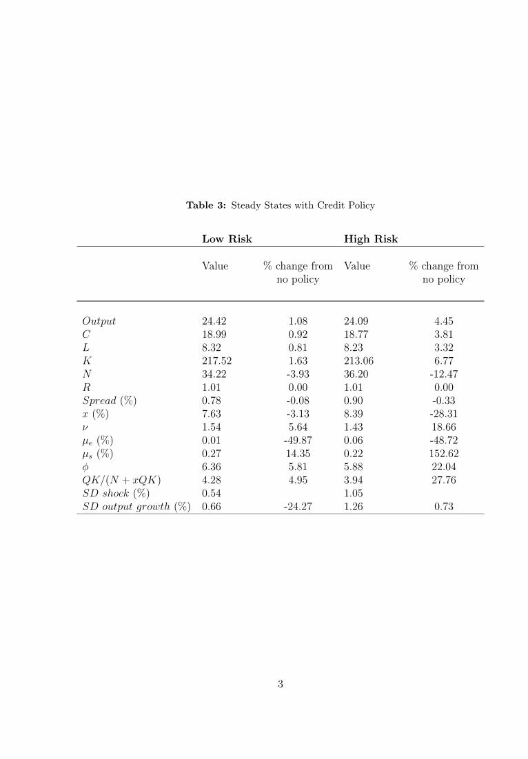
Table 3: Steady States with Credit Policy

Low Risk High Risk

Value % change from Value % change fromno policy no policy

Output 24.42 1.08 24.09 4.45C 18.99 0.92 18.77 3.81L 8.32 0.81 8.23 3.32K 217.52 1.63 213.06 6.77N 34.22 -3.93 36.20 -12.47R 1.01 0.00 1.01 0.00Spread (%) 0.78 -0.08 0.90 -0.33x (%) 7.63 -3.13 8.39 -28.31ν 1.54 5.64 1.43 18.66µe (%) 0.01 -49.87 0.06 -48.72µs (%) 0.27 14.35 0.22 152.62φ 6.36 5.81 5.88 22.04QK/(N + xQK) 4.28 4.95 3.94 27.76SD shock (%) 0.54 1.05SD output growth (%) 0.66 -24.27 1.26 0.73

3

Table 4: Welfare Effects of Policy

Welfare gain from no policyin consumption equivalents (%)

Efficiency cost of credit policy (bps) 0 50 100 200 400 800

Credit Policy 0.863 0.831 0.797 0.720 0.528 0.297Macroprudential Policy 0.007 0.007 0.007 0.007 0.007 0.007Macroprudential Policy with subsidy on Rk 0.253 0.253 0.253 0.253 0.253 0.253Macroprudential and Credit Policy 0.964 0.945 0.926 0.886 0.801 0.623

4

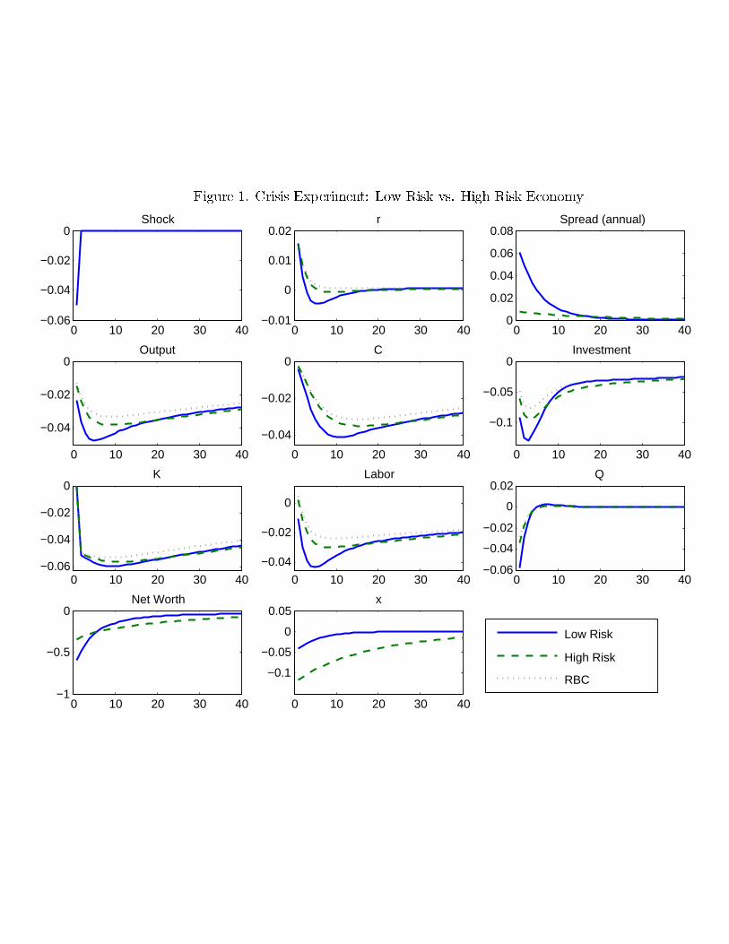
0 10 20 30 40−0.06

−0.04

−0.02

0Shock

0 10 20 30 40−0.01

0

0.01

0.02r

0 10 20 30 400

0.02

0.04

0.06

0.08Spread (annual)

0 10 20 30 40

−0.04

−0.02

0Output

0 10 20 30 40

−0.04

−0.02

0C

0 10 20 30 40

−0.1

−0.05

0Investment

0 10 20 30 40−0.06

−0.04

−0.02

0K

0 10 20 30 40

−0.04

−0.02

0

Labor

0 10 20 30 40−0.06

−0.04

−0.02

0

0.02Q

0 10 20 30 40−1

−0.5

0Net Worth

0 10 20 30 40

−0.1

−0.05

0

0.05x

Low Risk

High Risk

RBC

!#" $%#!&'(&)

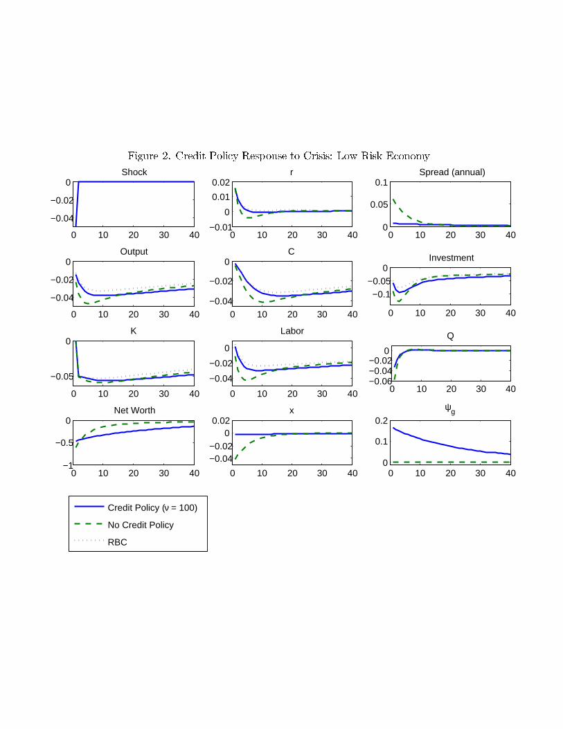
0 10 20 30 40

−0.04

−0.02

0Shock

0 10 20 30 40−0.01

0

0.01

0.02r

0 10 20 30 400

0.05

0.1Spread (annual)

0 10 20 30 40

−0.04

−0.02

0Output

0 10 20 30 40−0.04

−0.02

0C

0 10 20 30 40

−0.1−0.05

0Investment

0 10 20 30 40

−0.05

0K

0 10 20 30 40

−0.04

−0.02

0

Labor

0 10 20 30 40−0.06−0.04−0.02

0

Q

0 10 20 30 40−1

−0.5

0Net Worth

0 10 20 30 40

−0.04−0.02

00.02

x

0 10 20 30 400

0.1

0.2

ψg

Credit Policy (ν = 100)

No Credit Policy

RBC

!"#$%'& (

0 10 20 30 40−0.05

0

0.05Shock

0 10 20 30 400

10

20x 10

−3 r

0 10 20 30 400

5

x 10−3 Spread (annual)

0 10 20 30 40−0.04

−0.02

0Output

0 10 20 30 40−0.04

−0.02

0C

0 10 20 30 40−0.1

−0.05

0Investment

0 10 20 30 40

−0.05

0K

0 10 20 30 40−0.03−0.02−0.01

00.01

Labor

0 10 20 30 40−0.04

−0.02

0

Q

0 10 20 30 40

−0.4

−0.2

0Net Worth

0 10 20 30 40−0.2

−0.1

0

x

0 10 20 30 400

0.1

0.2ψg

Credit Policy (ν = 100)

No Credit Policy

RBC

!"#$%&' (

0 20 400

0.05

0.1

0.15

0.2

ψg

0 20 40−0.1

−0.05

0

0.05x

0 20 400

2

4

6

8x 10

−3 Spread (annual)

0 20 40−0.04

−0.03

−0.02

−0.01Output

0 20 40−0.04

−0.03

−0.02

−0.01

0C

0 20 40−0.1

−0.08

−0.06

−0.04

−0.02Investment

Anticipated Policy with ν = 100

Unanticipated Policy with ν = 20

RBC

"!#$%'&(*)+%, !-!.%$

0 10 20 30 400

0.05

0.1

0.15

0.2

ψg

0 10 20 30 40−0.1

−0.08

−0.06

−0.04

−0.02

0x

0 10 20 30 400

2

4

6

8x 10

−3 Spread (annual)

0 10 20 30 40−0.04

−0.03

−0.02

−0.01Output

0 10 20 30 40−0.04

−0.03

−0.02

−0.01

0C

0 10 20 30 40−0.1

−0.08

−0.06

−0.04

−0.02Investment

Credit Policy (ν=100), no Macroprudential Policy

Credit and Macroprudential Policy

RBC

!"!# $%&'()*#

0 10 20 30 40−0.06

−0.04

−0.02

0

0.02Shock

0 10 20 30 40

−0.05

0

0.05x

0 10 20 30 400

0.02

0.04

0.06

0.08Spread (annual)

0 10 20 30 40−0.05

−0.04

−0.03

−0.02

−0.01Output

0 10 20 30 40−0.04

−0.03

−0.02

−0.01

0C

0 10 20 30 40

−0.1

−0.05

0Investment

No Macroprudential Policy

Macroprudential Policy

RBC

!#" $#%! &(' )*%+$,%