financial conditions index (fci), inflation and growth

Financial conditions index (FCI), inflation and growth: Some evidence

Manamani SAHOO

University of Hyderabad, India [email protected]

Abstract. This paper first estimate financial conditions index (FCI) for India and then examines the empirical performance of the financial conditions index (FCI) to predict inflation and GDP growth. For optimal coverage of all major set of indicators, those which are determining the Indian economies, financial conditions, so we have broken financial conditions index into four sub-indices including major key indicator. The sub –indices of FCI include (i) short term rate of interest (CMR), (ii) exchange rate, (iii) housing price index (iv) FDI total inflow, each with equal weights. Based on granger causality and correlation test with quarterly data, the finding of this paper is the financial condition index is able to predict inflation bitterly.

Keywords: monetary conditions index, financial conditions index, housing price index. JEL Classification: B22, E44, E31, F43.

Theoretical and Applied EconomicsVolume XXIV (2017), No. 3(612), Autumn, pp. 147-172

148 Manamani Sahoo 1. Introduction

The main aim of monetary authority is to maintain monetary stability in economy with less inflation and more economic growth. For more monetary stability and proper functioning of the financial economy, sound financial conditions in an economy play an important role. Individual indicators like the exchange rate, short term interest rate, asset pricing and so on are the most important part of monetary policy. The lack of stability of these variables has affected economic growth and inflation of a country.

Monetary conditions index (MCI) is a weighted average of changes in monetary as well as financial variables in which the weights are intended to reflect the effect of these-variable on macro-economic variable such as inflation and economic growth. Freedman (1994) first proposed the construction of a monetary conditions index (MCI) and arguing that MCI being a weighted sum of the short-term interest rate and the exchange rate, is preferable to the interest rate and exchange rate alone as an operating target for a small open economy. In empirically we can say, an MCI is nothing but a simple weighted average of changes in an interest rate and an exchange rate relative to their, values in a base period. The estimated relative effects of interest rate and exchange rate on aggregate demand over some period is reflected by the weights given to those variables. Till now MCIs are, however, continue to be calculated by central banks and international organizations as an indicator for the stance of monetary policy. Currently MCIs are not only used as indicators of monetary conditions but also as operational short-run targets for monetary policy.

A financial conditions index is a simple device that combines moments in different financial variables such as short term interest rate, exchange rate, total FDI inflow and housing price. FCI is an extension of the monetary conditions index (MCI), including of total FDI inflows and housing price with later for covering of major set of indicator, which are related to the financial condition so that it becomes easy-to-understand information variable to financial markets. The study of financial conditions index (FCI) is of particular interest to the monetary authority since this can serve as information variables or even transmission variables, in the conduct of monetary policy. The relationships between the financial conditions index and other macro variables such as inflation and GDP growth can also be used to forecast changes in these latter variables. In this light, central banks are interested in choosing FCI that would act as useful indicators. For conduct of monetary policy and FCI can serve as a short-term operating target.

This paper first estimate financial conditions index (FCI) and then examines the empirical performance of the financial conditions index (FCI) to predict inflation and GDP growth. For optimal coverage of all major set of indicators, those which are determining the Indian economies, financial conditions, so I have broken financial conditions index into four sub-indices including major key indicator. The sub –indices of FCI include (i) short term rate of interest (CMR), (ii) exchange rate, (iii) housing price index (iv) FDI total inflow, each with equal weights.

Financial conditions index (FCI), inflation and growth: Some evidence 149

Extension of MCI to FCI

Individual indicators like the exchange rate, short-term interest rate, asset pricing and so on are the most important part of monetary policy. These variables are volatile over time to time and its volatility also depends on policy rules. The lack of stability of these variables has affected economic growth and inflation of a country. Due to inflation and economic growth are uncertain as measure by conditional variance has increased, it makes harder for forecasting inflation and growth. So, to identifying the appropriate indicators which could help for anticipating inflation and growth is important. From the prediction of inflation and economic growth central bank can take proper policy rules for it with a series of tools to anticipate future price pressured and change in economic activity. Individual indicators also have some limitations, one individual indicator is not sufficient for predicting the macro variable of the country as many other variables are also affecting it at the same time. So more than one individual variables are necessary for predicting the goal variable because these variables are simultaneously affecting to these goal variables. As inflation and economic growth influence of many macro-economic variables like short-term rate of interest, exchange rate, FDI and so on, so we need to take all these variables into account for prediction of inflation and economic growth.

The MCI is a composite index which measures changes in monetary as well as financial variables. In a pioneering study, Freedman (1994) constructed a MCI by combining both exchange rate and short term interest rate instead of taking single indicators. The estimated relative effects of interest rate and exchange rate on aggregate demand over some period are reflected by the weights given to those variables. Till now MCIs are, however, continue to be calculated by central banks and international organizations as an indicator of the stance of monetary policy. Currently, MCIs are not only used as indicators of monetary conditions but also as an operational short-run target for monetary policy.

So in simply MCI is a weighted average of short-term rate of interest (to capturing the interest rate-channel effect of monetary policy) and real exchange rate (to capturing the exchange rate channel effect of monetary policy).

So it's usually defined as:

MCIt = w1(rt – r0) + w2(et – e0) (1)

Where “MCIt” is the monetary conditions index for time period t (current time period), “r” is the short-term rate of interest, e is the natural logarithm of the exchange rate. In short-term comparison, an MCI can be constructed in real or nominal term because the difference is negligible. Whether we should give equal weight to all the variations or different weights to variables that depend on the importance of that variable to monetary policy. For assigning unequal weight, those weights are estimated by using the following strategies: a. Simulations on a structural macro-econometric model. b. Estimation of reduced–form aggregate demand equation. c. Estimation of structural vector auto-regression (VAR) system.

The financial conditions index is nothing, just an extension of the monetary conditions index. It is a simple device that combines moments in different financial variables such as

150 Manamani Sahoo short-term interest rate, exchange rate, total FDI inflow and housing price. It is an extension of the monetary conditions index (MCI), including of total FDI inflows and housing price with later for covering of a major set of indicator, which is related to the financial condition so that it becomes easy-to-understand information variable to financial markets. It is more efficient for prediction of inflation of economic growth than other individual variables and monetary conditions index, as it takes more relevant variables into accounts for prediction.

The financial conditions index can be express by

FCI = f (interest rate, exchange rate, HPI, FDI). (2)

Component of FCI

This work tries to construct the financial conditions index (FCI) and then after a predictive power of the FCI is checked by using econometric tools. The following components are selected for the Indian context.

i. Interest rate The interest rate channel is a most important tool of monetary policy, price level, output and employment are affected by a policy-induced changes in short-term rates of interest by a central bank. Expectation hypothesis describe, the rise in the short-term interest rate leads to rising in the long term interest rate, it is postulated by interest rate channel. This change affects the real interest rate directly and indirectly to the cost of capital because assumption taken for short-run is the sticky price. The interest rate mechanism is given emphasis on the real interest rate rather than the nominal interest rate, which is one most important feature of it. Interest rate-channel defines by a coming diagram of monetary expansion:

M↑ ⇒ir↓ ⇒ I↑ ⇒ Y↑

Where M↑ represents the increase in money supply (expansionary monetary policy) leads to a decrease in short-term real interest rate, which lowers the cost of capital so rise in investment, and finally increase in aggregate demand and employment.

ii. Exchange rate In an open economy and the coming of the flexible exchange rate, more attention has been given to monetary-transmission operating through exchange rate effect on net export. It also involves the effects of interest rate because the fall in the exchange rate for a currency occurs always with fall in domestic real interest rate, which leads to lower the value of that domestic currency. So domestic good becomes cheaper than foreign goods, by that causing an increase in net exports. The increase in net exports leads to increase aggregate output.

Exchange rate-channel defines by a coming diagram of monetary expansion:

M↑ ⇒ir↓ ⇒ E↑ ⇒ NX↑⇒Y↑

iii. Housing price in India Recent housing price fluctuation makes an important place of it in monetary policy. Transmission mechanisms of monetary policy beyond the standard interest rate and exchange rate-channel many other channels also affect it, we can give focus on housing


price due its recent fluctuation. Fluctuation in this housing price is likely to play an important role in how monetary policy has conducted.

A volatility in housing price directly or indirectly affects the households by affecting the value of wealth and hence its influence in the spending and borrowing decision of households. Stock and property prices recent volatility has renewed the interest towards the role of the asset for monetary policy. Forward moments in housing prices have raised the concerns about the appropriate stance of monetary policy with a different direction moment in financial markets. Housing prices are monitored monthly by the Reserve bank of India (RBI) in India. It is observed from the study of RBI for the last three years that in India annual average housing price increase is 20 per. So India has experienced significant housing market volatility in recent time like other countries.

Housing price index To measure the moment of single –family housing prices, the housing price index is used. It is a weighted, repeated–sales index to measure average changes in repeat sales or refinancing of some property. Rent paid for rented, self-owned house and rented free houses are taken in assembling the housing index.

The Housing price index is estimated by the reserve bank of India and it's based on the monthly consumer price index (CPI) for industrial workers. This index is a simple measure of housing price in India. The RBI compelling HPI individually for nine major cities as well as for the all-India level, these cities are Mumbai, Delhi, Chennai, Kolkata, Bengaluru, Lucknow, Ahmedabad, Jaipur and Kanpur. It used Laspeyres index based on transaction price and Q4:2008-09 taken as based year for it. Data’s for HPI are available in quarterly basis in official side of RBI.

iv. Total FDI inflow into India Foreign direct investment (FDI) refers to the inflow of foreign capital in terms of direct investment equity flows in the reporting country. It is just the sum of earnings, equity capital and other capital. To the prospect of skilled work force and good economic growth large amount of Foreign direct investment are attracted in opening economies than in highly regulated closed economies.

Financial and capital account liberalization in India facilitates to increasing capital flow into it. The post-globalization period has involved economic liberalization, it's opening-up economies to international trade and financial inflows. Total FDI inflows into India fluctuates time-to-time, which also impact to monetary policy. FDI inflow is more crucial to the economic growth enhancement (Hansan and Rand, 2006) because it brings technology, capital, and know how into the developing countries like India. And it also increases the stock of knowledge in the host countries by transferring knowledge through giving training to labor, transfer of skills, etc. It promotes more advanced technology into the host country, so it thought to open the export market and improve BOP in the host country. So India has also experienced a significant increase in total FDI inflow into it in recent time like other developing countries.

152 Manamani Sahoo Research gap

There are several studies found in the context of both advanced and emerging economies. However, there are very few studies done in the context of India to calculate FCI. The past studies have not accounted some of the important variables, such as FDI, housing price index, etc., in the construction of FCI. So there is a scope of the study to focus on expanding MCI to FCI by adding total FDI inflow and housing prices.

Objective of the study

For checking the short term financial conditions, financial conditions index (FCI) has served as a crucial indicator in Indian economy. The financial conditions Index is very helpful for forecasting the turning points in financial conditions. It helps in facilitating policy decision for a country by providing effective monitoring of current condition. Our study mainly focuses on three objectives: 1. Constructing a Financial conditions index (FCI) for India. 2. Testing the predictive ability of Financial conditions Index (FCI) for inflation. 3. Testing the predictive ability of Financial conditions Index (FCI) for GDP growth.

2. Model

Here we have described the methods of several time series tests and statistical tools. A detailed description is given about the procedure of testing the time series models. The methodology of unit root tests like Augmented dickey-fuller (ADF, 1984), Phillips-Perron (1988) and Kwiatkowski-Phillips-Schmidt-Shin (KPSS, 1992) and Granger causality are described thoroughly.

Human Development Index method (HDI) This method is a very useful method to make a composite index with more than one variable. HDI method first makes index for all individual variable by using formulas

xindex

3

Where x is the actual value of x variable, min(x) is the minimum value and max(x) is the maximum value the variable x can attain.

Then by giving equal weight to all those variables, the new composite index is constructed. As recommended by literature review and the theoretical support, we have taken four variables for construction of financial conditions index particularly, call money rate, which acting as a proxy for the rate of interest, exchange rate, housing price index (HPI) and foreign direct investment. Wholesale price index (WPI), which is acting as a proxy for inflation and GDP for factor price at constant cost are taken as goal variables. The reason behind using the housing price index and foreign direct investment in construction of FCI for their importance in the monetary transmission channel. For checking the order of integration of FCI, inflation, and GDP growth, we have used unit root test such as ADF, PP and KPSS. All these test results show that all the variables are of an order I-(1), so we


have taken first difference for all variable to make them stationary. The correlation test and causality test results suggest that there has a long run relation among FCI and inflation.

Testing of stationary and Unit-root The Unit root test is otherwise known as the test of stationary. Getting a significant co-efficient and high value of R2 (which is greater than the DW statistics) by regressing one variable upon another does not imply a meaningful relation exist among these two variable, there may be chance of spurious regression (that high value of R2 due to high and similar trend of these two variables). This unit root test was first introduced to economics by Granger and Newbold (1974). So for a meaningful relationship between two variable, both variable must be stationary. Stationary time series is one which is white noise (constant mean, constant variance and constant covariance of each variable given lag). Based on the fact that a non-stationary time series is defined by unit root, there is some method for testing of stationary such as Dickey and fuller (1979) augmented Dickey-fuller (1984), Phillips Perron (1988) and Kwiatkowski-Phillips-Schmidt-Shin (KPSS,1992).

i. Augmented Dickey-Fuller (ADF). The ADF test is superior to Dickey-Fuller (DF) because it takes the large and complicated set of time series models and it also can be applied where the error term is not white noise. It is used in a test, is a negative number. If it is more negative that means a high chance to reject the null hypothesis that there is unit-root at some confidence level.

The ADF can be written as:

ΔMt = θMt-1 + α1ΔMt-1 + α2ΔMt-2 + α3ΔMt-3 +… + αsΔMt-s + et (4)

Where ΔMt = Mt - Mt-1, “et” is the pure white noise error term (stochastic term) whose mean is equal to zero variance is constant and no auto-correlation with its lag, θ is a constant, α is the coefficient on a time trend and “s” is the lag order. To increase in coefficient standard error and reducing autocorrelation, lag “s” is chosen. Optimal lag “s” is chosen using both Akaike (AIC) and Schwartz’ Information criterion (SBIC).

ii. Phillips-Perron (PP) Unit Root test

Phillips-Perron (PP) Unit Root tests is an alternative method for testing unit root, when a time series is an integrated of order 1. It is the non-augmented Dicky-fuller (DF) by estimates. Phillips and Perrorn suggest this test in 1988. Phillips-Perron (PP) Unit Root tests is based on the dickey-fuller test, where the null hypothesis θ = 0 in ΔMt = θMt-1 + α1ΔMt-1 + α2ΔMt-2 + α3ΔMt-3 +...+ αsΔMt-s + et, and Δ is the first difference operator. It has just made the correction over the Augmented Dickey-Fuller (ADF), by making a non-parametric correlation to the t-statistics.

The Phillips-Perron (PP) test is based on following statistics:

Mt = α1Mt-1+ α2(t-T/2) + vt (5)

154 Manamani Sahoo Where T is the number of observations, v is the stochastic error term with Ewt = 0. In Phillips-Perron (PP) unit root test is better to ADF because on PP test there is no assumption like error terms are serially uncorrelated.

iii. Kwiatkowski-Phillips-Schmidt-Shin (KPSS) Test The KPSS test is an alternative method to both ADF and PP test for checking unit root. Unlike ADF and PP test where null hypothesis are taken as non-stationary, KPSS test stationarity in null hypothesis. Both with and with-out trend are reported in chapter-IV for capturing trend stationarity of the variables.

Correlation test The correlation coefficient measures the robustness of the relationship between two variables. The range of correlation coefficient is -1 to +1. So, correlation can be negative or positive, positive correlation Coefficient shows the relationship between two variables is positive means when one variable increase same time another variable also increasing, here we can take an example of income and consumption for simple understanding. Similarly, negative correlation coefficient reflects a negative relation between two variable, here we can take an example of price change of a commodity and demand of that commodity. If the correlation coefficient is zero for two variable, then that implies, there is no relation between those variables. If the value of correlation coefficient is closer to zero that implies there is a very weak relationship between two variables and if value closer to one (neglecting the negative sign) that showing a strong relation between two variable.

Granger-Causality test This test helps to decide whether one-time series is useful in forecasting another or not. But the argument of Civil Granger was that causality could be tested for by measuring the predictable capacity of a time series using the prior value of another time series. So simply it is a statistical concept and is based on the prediction. According to this test, if time series X is Granger-Causes another time series Y that implies past value of X should contain information about Y so that helps predict Y above and beyond the information contained in the prior value of “Y” alone.

To determine the direction of causality between the FCI, inflation and growth this test is done. This test was conducted with a view to knowing, which type of cause and effect relationship present between FCI, inflation, and real GDP growth. Wholesale price Index (WPI) is used as an indicator for inflation, while changes in economic are taken as the rate of growth of GDP. According to Mahdavi and Sohrabian (1989), the following two equations can be specified for inflation and FCI

(FCI)t = α + Σ βi(INF)t-1 + ΣTj(FCI)t-j + µt (6)

(INF)t = θ + Σ φi (FCI)t-1 + Σ ψj (INF)t-1 + ηt (7)

Where FCI is a Financial conditions index, the INF is inflation, i =1,…, m and j = 1,…, n for equation (6) where as for equation (7) i = 1,…, p and j = 1,…, q.

Four different hypotheses about the relations about the relationship between Inflation and Financial conditions Index (FCI) can be made based on OLS Coefficient (estimated) for equation (6) and (7).


A. Unidirectional Granger-causality from FCI and inflation B. Unidirectional Granger-causality from inflation and FCI C. Bidirectional or feedback causality. D. Independence between GDP and SP.

So by getting one of these results it seems possible to detect the causality relation between Financial conditions Index (FCI) and economic growth of a country.

3. Review of literature

An attempt is made to review the major national and international literature examining the construction and performance of the monetary conditions index and financial conditions index. There are few works done on the prediction of output growth and inflation using financial conditions index (FCI), monetary conditions index (MCI), and other economic indicators. This literature review reviews the use of single individual indicators such as the short-term rate of interest, real exchange rate and asset price.

A detailed survey is done regarding the procedure of testing the time series models and other statistical tools. We finally concluded composite index like MCI and FCI are better to predict macro variable like inflation and growth than single individual indicator like short-term interest rate, exchange rate, etc. But FCI gives more accurate results than MCI as it includes some more important financial variables.

Monetary conditions index (MCI) Giving a broad view on MCI, Costa (2000) discussed the interpretation of the monetary conditions index (MCI). She argues that MCI can be used as an indicator of stance of monetary policy. The MCI is calculated as a weighted average of short-term rate of interest and effective exchange rate. Weights are assigned, according to the relative importance of these variables in this economy. A reduction (increase) of the MCI corresponds to looser (tighter) monetary conditions. The MCI value lies between zero to hundred, the exact value MCI depends on the monetary conditions of that country.

R. Kannan et al. (2006) constructed a MCI for India by taking both interest rates-channel and exchange rate-channel simultaneously into account. . They took 1996Q2-2007Q1 data taken into account in this model. The result reveals that the monetary policy is influenced significantly by interest rate rather than exchange rate. Further, they show that MCI works as an effective tool to assess the stance of monetary policy has been more effective to put to gather than individual indicator in order to provide a better assessment of the stance of monetary policy and reveals its role as a leading indicator of economic activity and inflation. They're finding out “potential of MCI is a variable indicator of monetary policy in India supplementing the existing set of multiple indicators of monetary authority”.

Samantaraya (2009) also develops MCI for India. Due to Sevier limitation of an interest rate as an individual proxy of monetary policy, he extended FCI as an alternative proxy for it. Constructed MCI has taken three indices into account for its construction, where interest rates, exchange rate, monetary and banking aggregates and prices are taken as indicators for MCI. Here a broad information set of variables is taken for reflection of monetary policy

156 Manamani Sahoo appropriately. Construction of MCI was used for assessing the monetary policy impact on the macro variable inflation rate of growth and so on. A monthly MCI for the post-reform period (April 1996 – June 2008) is constructed in India by him. Here approach used for construction MCI is similar to that used by UNDP for the construction of some development indices such as HDI, GDI and so on. His findings were an MCI better indicator than traditional individual monetary policy indicator to capture the monetary policy stance for post-reform in India.

Xiong (2012) constructed the monetary conditions index for china over 1987Q1 – 2010Q2. Empirical results show that the MCIs has been useful in predicting future output growth and inflation over the short term and medium term in china. This article concludes with, derived MCI is informative than individual monetary variables for predicting inflation and output growth.

Gichuki and Moyi (2013) calculated MCI and tested its implications for monetary in Kenya. Here quarterly time series data for the time period 2000-2011 was taken for construction of MCI. Empirical results show the existence of co-integration between GDP, the real exchange rate, the claims on private sector and the short-term interest rate. It was finally concluded that MCI is a good indicator of inflation. Further, they argued that the interest rate and exchange rate movements can be controlled with the help of MCI.

Financial Conditions Index (FCI) Bank of Finland (2001) did a comparison between FCI and MCI using a group of countries from Western Europe. “Find a clear role for house prices, but a poorly determined relationship for stock prices”. These financial prices reflect wealth, by entry inter into key consumption and investment relationships and also the market expectation of future price and output development. FCI is better than other economic indicator data because it continuously updated as financial market trade. They have taken the different weight for the different indicator because all the indicators in FCI do not impact monetary policy to the same extent. “The results from using pooled data for most of the European Economic Area to explore the role of asset prices in explaining the output gap and inflation are promising. House prices, in particular, are helpful in providing information in addition to that contained in interest rates and the exchange rate”.

To propose a new index, Lack (2002) extended FCI to MCI including asset price and housing price. The result suggests that housing prices are capturing the wealth channel of monetary policy. It used CPI level effect as a proxy for inflation. For the calculating weight of FCI three strategies are used as most variables enter the model in nominal terms and FCI is mainly used for short-term comparison, shocks to nominal variables are simulated. He took annual data about 1974-2002 for housing price and showing the relation among MCIs, FCI and CPI inflation.

Gauthier et al. (2003) review on existing indices and prose several FCIs for Canada were done. Construction of several financial conditions indexes for Canada is done by using factor analysis and other tests. Each intended approach is to address one or more criticisms applied to MCIs and existing FCIs. They used different data for different model accordingly to need of that model, like monthly data for IS-curve based model, for better performance


of the model. Various FCIS estimation is done on the basis of their weights, dynamic correlation with output and inflation, their out-of-sample forecast and their in-sample fit in explaining output. They give emphasis to property and equity prices transmission mechanism through a wealth effect and a credit channel. Finally, they find FCI out performs the MCI in many criteria.

Montagnoli and Napolitano (2005) emphasized the interlink among asset price, inflation, and conduct of monetary policy. The main aim of monetary policy of central banks is to keep low inflation and more growth, and not possible to directly control inflation. So many instruments are used, like interest rate and the exchange rate for predicting inflation and growth. Interest rate and exchange rate are not sufficient indicators for predicting inflation and growth. FCI are constructed by taking asset's price into account as a good indicator for inflation and growth. For the construction of Financial Condition Indexes for four countries Kalman Filter algorithm is used. The main aim is to solve two problems the parameter inconstancy problem and the non-exogeneity of regressors. For the construction of FCI, the yearly data of most of the countries the sample for 1985-2005 are chosen. The results of the study suggest that the FCI Financial Condition Index is positively and statistically related to the setting of interest rate Federal Reserve, Bank of England and Bank of Canada. So, it is suggested that FCI could be an important tool to guide the course of monetary policy.

Beaton et al. (2009) did an expensive study on the relation among of financial conditions on US GDP growth. By using two growth base financial conditions indexes (FCI) they estimated the past and current shock to the financial variables on GDP growth. Structural vector error correction model is used for the construction of one of the FCI and for others they have taken large-scale macro-economic model. Tightening financial conditions have significantly dampened growth in the current year. They argue that final shock can have a larger impact in terms of higher real cost of interest rate.

Hatzius et al. (2010) proposed a new FCI measure by making comparison with single indicators. In that new FCI which built by them, three key innovations are made in terms of indicators, techniques. They have tried to find out the importance of FCI in prediction. They have mainly taken the quarterly data for construction of a model. They conclude that “in forecasting tests, the new FCI outperformed a variety of alternative measures in recent years”.

Ørbeck and Torvanger (2011) attempt to predict Norway GDP by using the financial conditional index. They take quarterly data of quarter 2 1980 to quarter 4 2005 for prediction of period of quarter 2 2006 to quarter 4 2014. Since 2007, the crises it contributed a downturn in the economy. The latest crisis demonstrated that how important financial conditions are for real economic growth and showed up that the predictive power from past indicators has been limited, so they are used FCI for prediction. For testing, forecasting power, they examine some alternative forecast as a benchmark. They used PC approach and VAR model for calculation of weight. The result was the best FCI model based on RMSE is our static model, but chosen on MAPE the best model is the FCI with lag one. They emphasized on RMSE criterion due to the assumption underlying OLS estimate.

158 Manamani Sahoo Chow (2012) studies the importance of FCI in guiding the monetary policy in Singapore. Real Interest rates, real exchange rates, real credit expansion and asset price (real stock prices and real house prices) are taken as a key component of FCI. Quarterly data of every component on it are taken of Q1: 1978 to Q1: 2011 for the construction of financial conditions index for Singapore. The causality test indicates that the FCI is helpful in predicting inflation from sample.

Wang et al. (2012) constructed financial conditions index (FCI) by using a regression model based on Support Vector Machine. The main aim to link between the financial indicator and future inflation. Here the more advanced machine learning method comparison to traditional econometric model is used to find accurate forecasts of future inflation in the small data base. AS money supply play an important place in monetary policy so they included in it. So short-term interest rates, money supply (M2), real estate prices, stock prices and real effective exchange rate are used as an indicator in FCI. A monthly data from July 2010 to December 2010 for all indicators are taken for construction of FCI. “The experiment result shows that FCI (SVRs) performs better than VAR impulse response analysis. As a result, our model based on support vector regression in the construction of the FCI is appropriate”.

IMF (2012) constructed the FCI for South Africa. Principal component analysis and Kalman filter approach are used for extracting the index. They calculate a common for the period of 1999q1 and 2001q4 by including the financial indicator, which is exogenous to South Africa and the global financial condition and indicated that related to South Africa. They divide variable as the global and domestic factor. The comparison is done among pre-crisis, financial crisis and post-crisis period. The predictive power of the FCI is tested by using out-of-sample forecast and an in-sampler exercise. Finally, the results indicate that “both the PCA and Kalman filtered FCI performed better as a leading indicator of real activity relative to the SARB’s leading indicator, and to an autoregressive model of GDP growth”.

ADB (2013) constructed the financial conditions index for five Asian economies, using a principal analysis (PCA) methodology. Financial market and the real economy are closely linked by affecting one to another. FCIs are constructed for five Asian economies and also regional FCI for the individual economy are constructed. Principal component analysis (PCA) methodology is used for calculation of weights. FCI measure financial shocks so it a better predictor of future economic activity. For the construction of FCI quarterly data for 1970-2011 are taken into account. Finally a comparison among New index and single financial indicators for testing predictive power. The results suggest that “new FCI can be quite helpful in gauging of the future state of the economy, although forecasting accuracy appears to be higher for countries with a complete range of financial data”. Finally, it is found that countries having a larger dataset available have enjoyed higher predictive power in FCI. Domestic and Krznar (2013) constructed the Financial Conditions Index (FCI) for Croatia, together with two subcomponents domestic and foreign. In a small and open economy, real and financial developments dependent on domestic factors, also heavily depend on global economic and financial conditions. So this paper analyzes interrelation between domestic and external financial conditions and economic activity. Vector auto-


regression (VAR) is used by them for an estimation of interdependence between financing conditions and real economic activity in Croatia. The result of VAR shows, FCI is capable for a forecast of domestic GDP and external financial conditions. Variance decomposition was also estimated by them with these same variables, and the result was almost same as VAR model.

Shankar (2014) emphasizes more on information asymmetry in financial markets, especially at times of crises. To overcome the information asymmetry FCI is constructed. For calculation, he used monthly data between January 2004 and August 2013. According to him, classification of financial markets are money market, bond market, foreign exchange market and equity market, and each market plays a significant role in monetary transmission. He used principal component analysis (PCA) for calculation of weights of FCI. The final conclusion was as compared to any other index, FCI should be updated sufficiently often enough so that it is able to capture the changes in market structure bitterly.

Zheng and Yu (2014) constructed the financial conditions index (FCI) by taking interest rate, exchange rate, stock price and house price selected as the variables and the percent change rate of the variable as an indicator. Therefore, it is very important to construct China’s FCI for investigating China’s economic and financial situation more precisely. They select the percent change rate of the variable as indicators to construct the FCI, which not only effectively describes the indicators, but also avoid errors arising from of gap measuring. Principal Component Analysis and Dynamic Factor methods are both introduced to build FCI. FCIs constructed by the two methods are compared, and the robustness of the FCI are tested. Five variables, money supply, interest rates, exchange rates, stock index and house price index, are selected to construct FCI. All of these indicators are taken monthly data of January 1998 – June 2013. FCI can better reflect the situation of China's financial operation, and can better predict the economic trends. Therefore, FCI can serve as an important reference index, whose performance is superior to a single financial variable.

Angelopoulou et al. (2014) attempted to calculate FCI in the euro Areas. The sample period covers 2003 to 2011. While calculating FCIs they have separated index by including FCI with monetary policy variables and FCI with non-monetary policy variables. The empirical findings support in favour of new FCI. The index outperform over individual indicator to predict the macro outcomes.

Charleroy and Stemmer (2014) formulated FCI for a large sample of emerging economies. They tested FCI’s forecasting applicability for business cycles. They used vector auto-regressive model for the construction of FCI. The study uses data, which ranges from January 2001 and March 2013. They find that FCI has significant power in predicting the growth than any other indicators.

CII and IBA (2015) did a survey of prime banks and other intermediaries to construct financial Conditions Index. For constructing financial conditions index CII-IBA used purchasing managers index. FCI broken into four subs induces including four indicators under each. Equal weight taken for each indices are: cost of fund index, fund liquidity index, external financial linkage index, economic activity index.

160 Manamani Sahoo 5. Estimation of financial conditions index for India

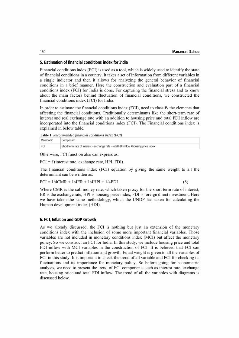
Financial conditions index (FCI) is used as a tool, which is widely used to identify the state of financial conditions in a country. It takes a set of information from different variables in a single indicator and then it allows for analyzing the general behavior of financial conditions in a brief manner. Here the construction and evaluation part of a financial conditions index (FCI) for India is done. For capturing the financial stress and to know about the main factors behind fluctuation of financial conditions, we constructed the financial conditions index (FCI) for India.

In order to estimate the financial conditions index (FCI), need to classify the elements that affecting the financial conditions. Traditionally determinants like the short-term rate of interest and real exchange rate with an addition to housing price and total FDI inflow are incorporated into the financial conditions index (FCI). The Financial conditions index is explained in below table.

Table 1. Recommended financial conditions index (FCI)

Mnemonic Component

FCI Short term rate of interest +exchange rate +total FDI inflow +housing price index

Otherwise, FCI function also can express as:

FCI = f (interest rate, exchange rate, HPI, FDI).

The financial conditions index (FCI) equation by giving the same weight to all the determinant can be written as:

FCI = 1/4CMR + 1/4ER + 1/4HPI + 1/4FDI (8)

Where CMR is the call money rate, which taken proxy for the short term rate of interest, ER is the exchange rate, HPI is housing price index, FDI is foreign direct investment. Here we have taken the same methodology, which the UNDP has taken for calculating the Human development index (HDI).

6. FCI, Inflation and GDP Growth

As we already discussed, the FCI is nothing but just an extension of the monetary conditions index with the inclusion of some more important financial variables. Those variables are not included in monetary conditions index (MCI) but affect the monetary policy. So we construct an FCI for India. In this study, we include housing price and total FDI inflow with MCI variables in the construction of FCI. It is believed that FCI can perform better to predict inflation and growth. Equal weight is given to all the variables of FCI in this study. It is important to check the trend of all variable and FCI for checking its fluctuations and its importance for monetary policy. So before going for econometric analysis, we need to present the trend of FCI components such as interest rate, exchange rate, housing price and total FDI inflow. The trend of all the variables with diagrams is discussed below.


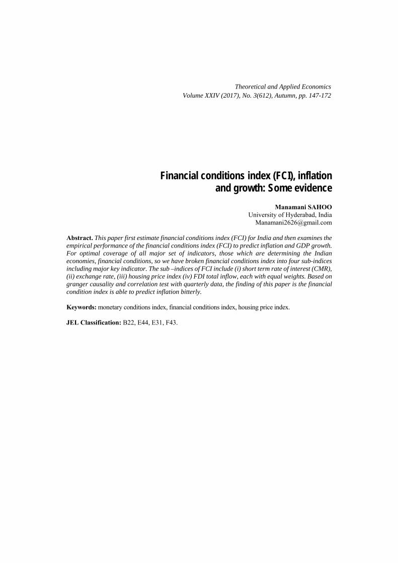
Short-term interest rate (call money rate) Short term interest rates are generally the rate at which borrowing for a short-term are effected between financial institutions. The Short-term interest rate is measured as a percentage and these are generally the average of daily rates. Short term interest rates are based on the three-month money market rates, typically the money market rate and treasury bill rate. Here we used to call money rate as the proxy for the short term interest rate. Call money rate (CMR) is the rate at which commercial banks and financial institutions lend to and borrow from the money market during the short period.

i. Trend in call money rate The trend of the call money rate is shown in the graph-1 where the X-axis present the time horizon and Y-axis presents the call money rate. Being a measure of liquidity availability and thus reflects the short-term costs of available funds, it has shown a greater volatility and fluctuated widely due to supply and demand sides of the Indian money market. Starting from about 8% during the last quarter of 2008-2009 CMR has fallen drastically to below 4% during the quarter 2 of 2009-2010 owing to the effects of the global meltdown. Further, it remained stable till the quarter 1 of the following year and then showed a steady increase till the Q1 of 2012-2013 owing to macroeconomic stability. The rate again followed the declining trend till Q2 of 2012-2013 making an average of around 4% during the year and then with a steep increase in Q1 to Q3 of 2013-2014 and relative falling trend during the recent period; the rate is averaged to around 7.20%.

Figure 1. Call Money Rate

3

4

5

6

7

8

9

10

Q4:

08-0

9Q

1:

09-1

0Q

2:

09-1

0Q

3:

09-1

0Q

4:

09-1

0Q

1:1

0-11

Q2:1

0-11

Q3:1

0-11

Q4:1

0-11

Q1:1

1-12

Q2:1

1-12

Q3:1

1-12

Q4:1

1-12

Q1:1

2-13

Q2:1

2-13

Q3:1

2-13

Q4:1

2-13

Q1:1

3-14

Q2:1

3-14

Q3:1

3-14

Q4:1

3-14

Q1:1

4-15

Q2:1

4-15

Q3:1

4-15

Q4:1

4-15

Q1:1

5-16

Q2:1

5-16

Q3:1

5-16

Q4:1

5-16

CMR

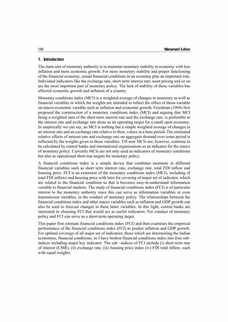
Exchange rate In simple, the exchange rate can be defined as the price of domestic currency in the terms of any other countries currency. So there are basically two components of the exchange rate, one is domestic currency and foreign currency.

162 Manamani Sahoo i. we cannot present exchange rate of more than two currencies in a two-dimensional plane, we take the exchange rate between the rupee and the US dollar. It is observed that the dollar is the foremost reserve currency in the world. Like the currencies of major countries, the Indian rupee too witnessed the effects of global financial crisis as is evident from the Figure 2. The rate increases from around 49 US dollar during the last quarter of crisis to around 60 US dollar till the last quarter of following year. The rate declined steeply to a level of around 45 during the first quarter of 2010-2011 and then remained more or less stable during the second quarter of 2011-2012 due to various policy regulations of the Reserve Bank. The rate again followed an upward depreciating trajectory of domestic currency with few down movements at certain instances, reaching to the peak level of 68.80 during September 2013 due to the global uncertainties, fall in oil prices, fall in FIIs, Indian trade deficit, etc. The rate continued its depreciating mode even during the recent period and has remained more or less around 66.59 during 2015-2016.

Figure 2. Exchange rate

44

48

52

56

60

64

Q4:

08-

09Q

1: 0

9-10

Q2:

09-

10Q

3: 0

9-10

Q4:

09-

10Q

1:10

-11

Q2:

10-1

1Q

3:10

-11

Q4:

10-1

1Q

1:11

-12

Q2:

11-1

2Q

3:11

-12

Q4:

11-1

2Q

1:12

-13

Q2:

12-1

3Q

3:12

-13

Q4:

12-1

3Q

1:13

-14

Q2:

13-1

4Q

3:13

-14

Q4:

13-1

4Q

1:14

-15

Q2:

14-1

5Q

3:14

-15

Q4:

14-1

5Q

1:15

-16

Q2:

15-1

6Q

3:15

-16

Q4:

15-1

6

ER

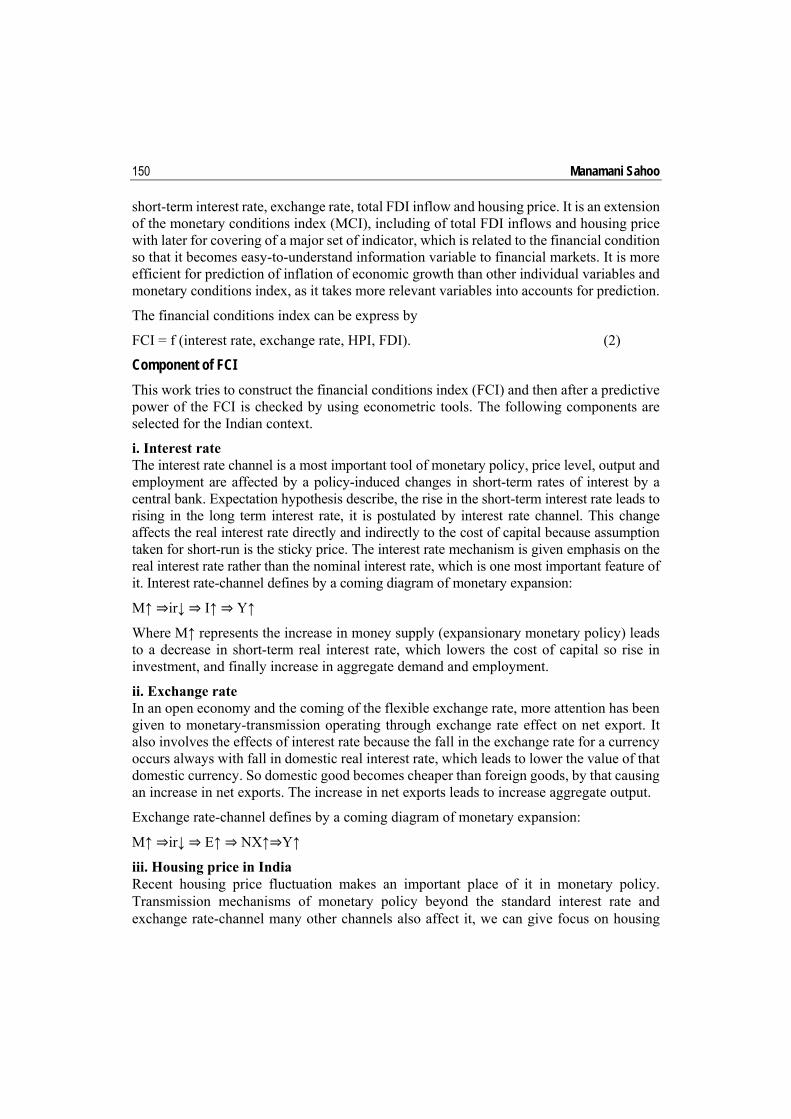
Housing price index The housing price index (HPI) of a country measures changes in the price of residential housing. For estimating change in the mortgage defaults, prepayments and housing affordability housing price index price index provide a tool.

Trends in housing price index Housing price index in India has shown an increasing trend over the years reached its peak in 2012-2013 and then stabilized during the recent period. The housing price inflation, as measured by RPPI, has swollen from a relatively moderate level of 4% during quarter 1 of 2011-2012 to a galloping figure of 28% during quarter 3 of 2012-2013 but the trend has reversed thereafter and has again reached to the level of 4% during the recent period (RBI, 2015).


Figure 3. Housing Price Index

60

80

100

120

140

160

180

200

220

240

Q4

: 08

-09

Q1

: 09

-10

Q2

: 09

-10

Q3

: 09

-10

Q4

: 09

-10

Q1:

10-1

1Q

2:10

-11

Q3:

10-1

1Q

4:10

-11

Q1:

11-1

2Q

2:11

-12

Q3:

11-1

2Q

4:11

-12

Q1:

12-1

3Q

2:12

-13

Q3:

12-1

3Q

4:12

-13

Q1:

13-1

4Q

2:13

-14

Q3:

13-1

4Q

4:13

-14

Q1:

14-1

5Q

2:14

-15

Q3:

14-1

5Q

4:14

-15

Q1:

15-1

6Q

2:15

-16

Q3:

15-1

6Q

4:15

-16

HPI

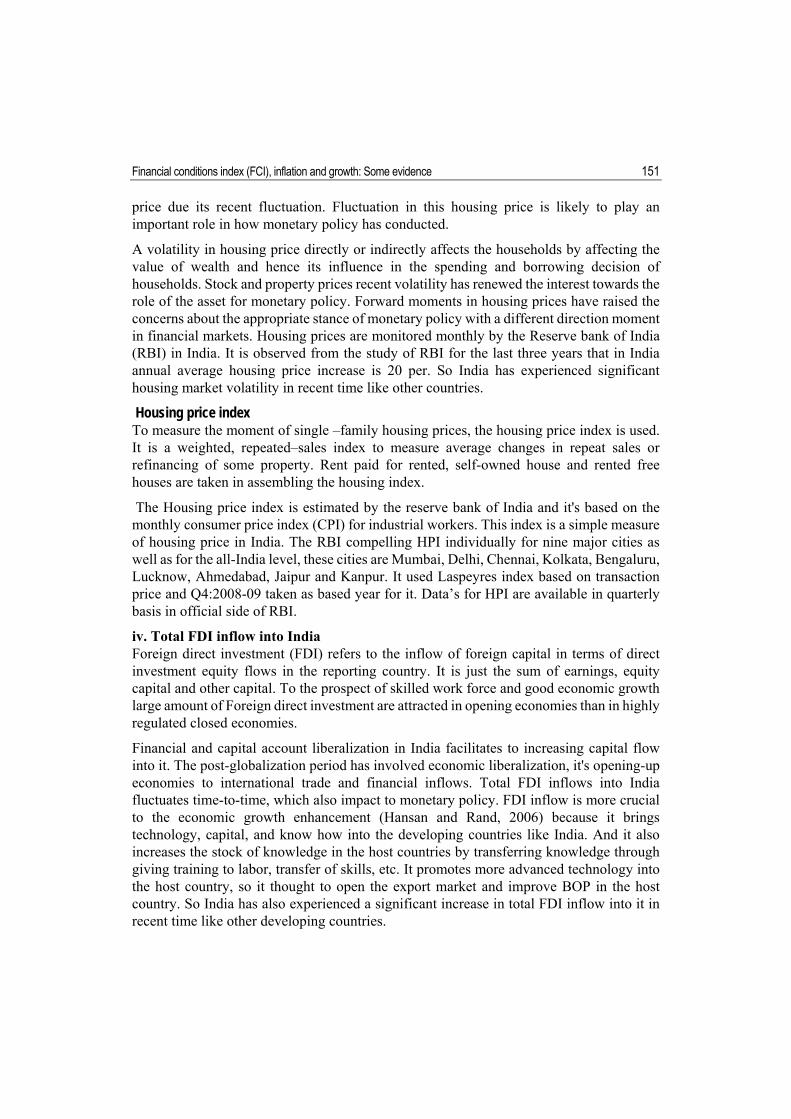
Foreign direct investment (FDI) A foreign direct investment (FDI) is a direct investment equity flows into the reporting country from the company or entity of other countries. The trend of the FDI is explained in below.

i. Trend in total FDI inflow into India India being a developing country has usually remained dependent on foreign inflows and has adopted various policies and strategies to manage them. Taking the synoptic view of Figure 4, it is evident that FDI on an average has shown an upward movement during the period under consideration with various ups and downs. Starting from the depressed conditions of 2008-09 the economy receives the increased foreign inflows after macroeconomic stabilisation, but there after it showed a decline till the first quarter of 2011-2012 and marked the highest value during the second quarter of same year owing to increased openness to the external world and serving as the investment destination of the world. But despite the various efforts on the part of the government, FDI declined during 2012-2013 although showed some signs of recovery during 2013-2014 and then followed an upward trajectory during 2014-2015 due to the launching of “make in India” program during September 2014. The favorable policy regime and the sound business environment has helped India to witness an increased foreign flows in the following year as well.

164 Manamani Sahoo Figure 4. Foregn direct Investment

100,000

200,000

300,000

400,000

500,000

600,000

700,000

Q4:

08-

09

Q1:

09-

10

Q2:

09-

10

Q3:

09-

10

Q4:

09-

10

Q1:

10-1

1

Q2:

10-1

1

Q3:

10-1

1

Q4:

10-1

1

Q1:

11-1

2

Q2:

11-1

2

Q3:

11-1

2

Q4:

11-1

2

Q1:

12-1

3

Q2:

12-1

3

Q3:

12-1

3

Q4:

12-1

3

Q1:

13-1

4

Q2:

13-1

4

Q3:

13-1

4

Q4:

13-1

4

Q1:

14-1

5

Q2:

14-1

5

Q3:

14-1

5

Q4:

14-1

5

Q1:

15-1

6

Q2:

15-1

6

Q3:

15-1

6

Q4:

15-1

6

FDI

Financial conditions index (FCI) Financial Conditions Index (FCI) is an indicator variable, which has four components such as the short-term rate of interest, exchange rate, FDI, HPI. As any regression analysis needs stationarity check of all the variables to avoid spurious regression, similarly checking of the trend is necessary for knowing prior information about the variables.

i. Trend in Financial conditions index (FCI) The trend of the FCI is shown in the Figure 5. Taking the synoptic view of Figure 5, it is evident that FCI on an average has shown an upward movement. FCI has declined during 2008-09 although showed some signs of recovery during Q1-Q3 of 2009-10. But then again followed a downturn till Q1 of 2010-2011. FCI showed an increasing during 2012-13 although showed some signs of depression during 2013-14 but then after sudden recovery started and finally it stabilized during the recent periods.

Figure 5. Financial Conditions Index

.0

.1

.2

.3

.4

.5

.6

.7

.8

.9

Q4

: 08

-09

Q1

: 09

-10

Q2

: 09

-10

Q3

: 09

-10

Q4

: 09

-10

Q1

:10

-11

Q2

:10

-11

Q3

:10

-11

Q4

:10

-11

Q1

:11

-12

Q2

:11

-12

Q3

:11

-12

Q4

:11

-12

Q1

:12

-13

Q2

:12

-13

Q3

:12

-13

Q4

:12

-13

Q1

:13

-14

Q2

:13

-14

Q3

:13

-14

Q4

:13

-14

Q1

:14

-15

Q2

:14

-15

Q3

:14

-15

Q4

:14

-15

Q1

:15

-16

Q2

:15

-16

Q3

:15

-16

Q4

:15

-16

FCI


7. Empirical analysis

In this section, we analyze the predictive capacity of financial conditions index (FCI) to forecast inflation and growth using some econometric tools. The results of all those econometric models are given below in one by one.

Unit-Root test result For this study, we choose Augmented Dickey-fuller (ADF, 1984), Phillips-Perron (PP, 1988) test and Kwiatkowski-Phillips-Schmidt-Shin(KPSS, 1992)

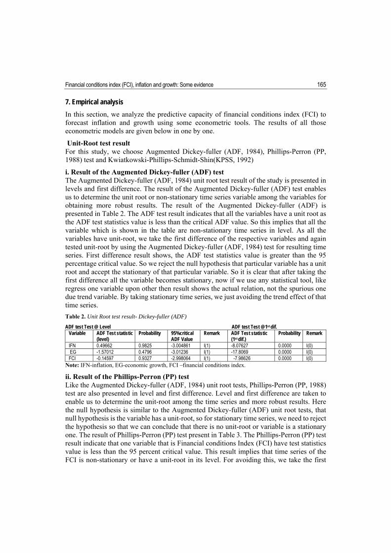
i. Result of the Augmented Dickey-fuller (ADF) test The Augmented Dickey-fuller (ADF, 1984) unit root test result of the study is presented in levels and first difference. The result of the Augmented Dickey-fuller (ADF) test enables us to determine the unit root or non-stationary time series variable among the variables for obtaining more robust results. The result of the Augmented Dickey-fuller (ADF) is presented in Table 2. The ADF test result indicates that all the variables have a unit root as the ADF test statistics value is less than the critical ADF value. So this implies that all the variable which is shown in the table are non-stationary time series in level. As all the variables have unit-root, we take the first difference of the respective variables and again tested unit-root by using the Augmented Dickey-fuller (ADF, 1984) test for resulting time series. First difference result shows, the ADF test statistics value is greater than the 95 percentage critical value. So we reject the null hypothesis that particular variable has a unit root and accept the stationary of that particular variable. So it is clear that after taking the first difference all the variable becomes stationary, now if we use any statistical tool, like regress one variable upon other then result shows the actual relation, not the spurious one due trend variable. By taking stationary time series, we just avoiding the trend effect of that time series.

Table 2. Unit Root test result- Dickey-fuller (ADF)

ADF test Test @ Level ADF test Test @1st dif. Variable ADF Test statistic

(level) Probability 95%critical

ADF Value Remark ADF Test statistic

(1st dif.) Probability Remark

IFN 0.49662 0.9825 -3.004861 I(1) -8.07627 0.0000 I(0) EG -1.57012 0.4796 -3.01236 I(1) -17.8069 0.0000 I(0) FCI -0.14597 0.9327 -2.998064 I(1) -7.98626 0.0000 I(0)

Note: IFN-inflation, EG-economic growth, FCI –financial conditions index.

ii. Result of the Phillips-Perron (PP) test Like the Augmented Dickey-fuller (ADF, 1984) unit root tests, Phillips-Perron (PP, 1988) test are also presented in level and first difference. Level and first difference are taken to enable us to determine the unit-root among the time series and more robust results. Here the null hypothesis is similar to the Augmented Dickey-fuller (ADF) unit root tests, that null hypothesis is the variable has a unit-root, so for stationary time series, we need to reject the hypothesis so that we can conclude that there is no unit-root or variable is a stationary one. The result of Phillips-Perron (PP) test present in Table 3. The Phillips-Perron (PP) test result indicate that one variable that is Financial conditions Index (FCI) have test statistics value is less than the 95 percent critical value. This result implies that time series of the FCI is non-stationary or have a unit-root in its level. For avoiding this, we take the first

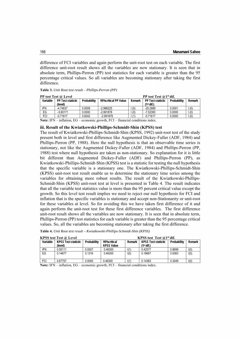
166 Manamani Sahoo difference of FCI variables and again perform the unit-root test on each variable. The first difference unit-root result shows all the variables are now stationary. It is seen that in absolute term, Phillips-Perron (PP) test statistics for each variable is greater than the 95 percentage critical values. So all variables are becoming stationary after taking the first difference.

Table 3. Unit Root test result – Phillips-Perron (PP)

PP test Test @ Level PP test Test @1st dif. Variable PP Test statistic

(level) Probability 95%critical PP Value Remark PP Test statistic


IFN -4.74637 0.0009 -2.986225 I (0) -20.2689 0.0001 I (0) EG - 6.60171 0.0000 -2.991878 I (0) -7.52393 0.0000 I (0) FCI -0.71617 0.8242 -2.991878 I (1) -0.71617 0.0000 I (0)

Note: IFN – inflation, EG – economic growth, FCI – financial conditions index.

iii. Result of the Kwiatkowski-Phillips-Schmidt-Shin (KPSS) test The result of Kwiatkowski-Phillips-Schmidt-Shin (KPSS, 1992) unit-root test of the study present both in level and first difference like Augmented Dickey-Fuller (ADF, 1984) and Phillips-Perron (PP, 1988). Here the null hypothesis is that an observable time series is stationary, not like the Augmented Dickey-Fuller (ADF, 1984) and Phillips-Perron (PP, 1988) test where null hypothesis are taken as non-stationary. So explanation for it is little bit different than Augmented Dickey-Fuller (ADF) and Phillips-Perron (PP), as Kwiatkowski-Phillips-Schmidt-Shin (KPSS) test is a statistic for testing the null hypothesis that the specific variable is a stationary one. The Kwiatkowski-Phillips-Schmidt-Shin (KPSS) unit-root test result enable us to determine the stationary time series among the variables for obtaining more robust results. The result of the Kwiatkowski-Phillips-Schmidt-Shin (KPSS) unit-root test at level is presented in Table 4. The result indicates that all the variable test statistics value is more than the 95 percent critical value except the growth. So this level test result implies we need to reject our null hypothesis for FCI and inflation that is the specific variables is stationary and accept non-Stationarity or unit-root for these variables at level. So for avoiding this we have taken first difference of it and again perform the unit-root test for these first difference variables. The first difference unit-root result shows all the variables are now stationary. It is seen that in absolute term, Phillips-Perron (PP) test statistics for each variable is greater than the 95 percentage critical values. So, all the variables are becoming stationary after taking the first difference.

Table 4. Unit Root test result – Kwiatkowski-Phillips-Schmidt-Shin (KPSS)

KPSS test Test @ Level KPSS test Test @1st dif. Variable KPSS Test statistic

(level) Probability 95%critical

KPSS Value Remark KPSS Test statistic


IFN 0.55111 0.0007 0.46300 I(1) 0.42577 0.8699 I(0) EG 0.14677 0.1316 0.46300 I(0) 0.18667 0.9363

I(0)

FCI 0.67757 0.0000 0.46300 I(1) 0.14363 0.3049 I(0) Note: IFN – inflation, EG – economic growth, FCI – financial conditions index.


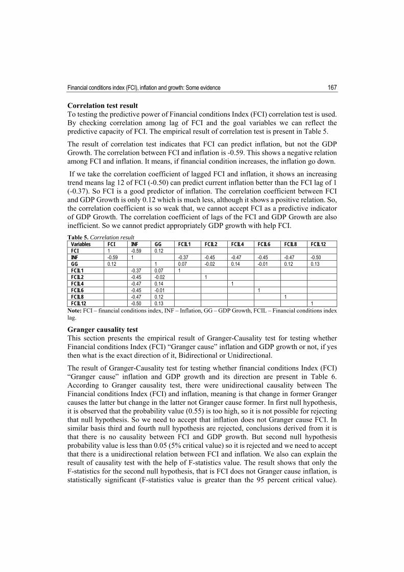
Correlation test result To testing the predictive power of Financial conditions Index (FCI) correlation test is used. By checking correlation among lag of FCI and the goal variables we can reflect the predictive capacity of FCI. The empirical result of correlation test is present in Table 5.

The result of correlation test indicates that FCI can predict inflation, but not the GDP Growth. The correlation between FCI and inflation is -0.59. This shows a negative relation among FCI and inflation. It means, if financial condition increases, the inflation go down.

If we take the correlation coefficient of lagged FCI and inflation, it shows an increasing trend means lag 12 of FCI (-0.50) can predict current inflation better than the FCI lag of 1 (-0.37). So FCI is a good predictor of inflation. The correlation coefficient between FCI and GDP Growth is only 0.12 which is much less, although it shows a positive relation. So, the correlation coefficient is so weak that, we cannot accept FCI as a predictive indicator of GDP Growth. The correlation coefficient of lags of the FCI and GDP Growth are also inefficient. So we cannot predict appropriately GDP growth with help FCI.

Table 5. Correlation result Variables FCI INF GG FCIL1 FCIL2 FCIL4 FCIL6 FCIL8 FCIL12 FCI 1 -0.59 0.12 INF -0.59 1 -0.37 -0.45 -0.47 -0.45 -0.47 -0.50 GG 0.12 1 0.07 -0.02 0.14 -0.01 0.12 0.13 FCIL1 -0.37 0.07 1 FCIL2 -0.45 -0.02 1 FCIL4 -0.47 0.14 1 FCIL6 -0.45 -0.01 1 FCIL8 -0.47 0.12 1 FCIL12 -0.50 0.13 1

Note: FCI – financial conditions index, INF – Inflation, GG – GDP Growth, FCIL – Financial conditions index lag.

Granger causality test This section presents the empirical result of Granger-Causality test for testing whether Financial conditions Index (FCI) “Granger cause” inflation and GDP growth or not, if yes then what is the exact direction of it, Bidirectional or Unidirectional.

The result of Granger-Causality test for testing whether financial conditions Index (FCI) “Granger cause” inflation and GDP growth and its direction are present in Table 6. According to Granger causality test, there were unidirectional causality between The Financial conditions Index (FCI) and inflation, meaning is that change in former Granger causes the latter but change in the latter not Granger cause former. In first null hypothesis, it is observed that the probability value (0.55) is too high, so it is not possible for rejecting that null hypothesis. So we need to accept that inflation does not Granger cause FCI. In similar basis third and fourth null hypothesis are rejected, conclusions derived from it is that there is no causality between FCI and GDP growth. But second null hypothesis probability value is less than 0.05 (5% critical value) so it is rejected and we need to accept that there is a unidirectional relation between FCI and inflation. We also can explain the result of causality test with the help of F-statistics value. The result shows that only the F-statistics for the second null hypothesis, that is FCI does not Granger cause inflation, is statistically significant (F-statistics value is greater than the 95 percent critical value).

168 Manamani Sahoo So this null hypothesis was rejected and need to accept that FCI granger causes inflation. Other F-statistics values are showing statistically insignificant, as F-statistics values are less than the 95 percent critical value for all three null hypothesis. So we cannot reject these null hypothesizes. Thus, the conclusion derives is that inflation does not Granger Cause Financial conditions Index FCI, and there is no causality among Financial conditions Index (FCI) and GDP Growth.

Table 6. Causality test result Null hypothesis F- statistics Prob. Granger cause Direction INFLATION does not Granger Cause FCI 0.62427 0.5469 No None FCI does not Granger Cause INFLATION 4.29498 0.0299 Yes Uniderectional

(FCI → INFLATION) GDP growth does not Granger Cause FCI 1.99465 0.1650 No None FCI does not Granger cause GDP growth 0.91631 0.4179 No None

Note: GDP – Gross domestic product, FCI – financial conditions index, Prob. – probability. Financial conditions Index (FCI), Inflation and GDP Growth

Before discussing the conclusion of the study we need to explain the objective of our study with regard to our test results. The most important objective of our study is to test the predictive capacity of the financial Conditions Index (FCI) for inflation and GDP growth. This is nothing but the testing of whether the FCI is a good indicator or not.

Based on the causality and correlation test result, we argue that higher the FCI, the lower the inflation in a country and FCI do not content much information about the GDP growth. So we cannot say the exact relation among them. For clear understanding, we need to explain the test result. First, we present the predictive power of the FCI for inflation and the relation between them and then the predictive power of the FCI for GDP Growth and their relations.

Inflation means an increase in the general price level. It is affected by many variables simultaneously. Till a certain point inflation contribute positively to the economic growth and after that inverse relation will occur in a country. So in many developing countries main aim is to maintain less inflation with more economic growth for monetary stability. For that properly prediction of inflation is needed. Fluctuation in inflation can be explained better from the Figure 6. It shows that India has most often suffered from the problem of inflation either because of monetary factors or by supply shocks. As is evident from the graph below, WPI has shown various ups and downs during the period considered. Starting with a lower value during the last quarter of 2008-2009, it jumped steeply in the following quarter owing to meltdown effects. As the economy stabilized to some extent WPI also showed the signs of decline with some gyrations in between the year of 2009-2010. With the increased food prices, rise in prices of primary articles and fuel costs, etc. during 2010-2011, WPI has again witnessed the upward movements and then showed some decline during the following years due to moderation in international commodity prices, lowering crude oil prices and continuous tightening of monetary policy by the reserve bank.

If we take the causality test result, its showing there is a unidirectional relation among FCI and inflation and that direction is FCI cause inflation. It means any change in the FCI cause changes in inflation but the reverse is not occurring. The Correlation test result reflects that there is a strong correlation between FCI and inflation. And it also shows that using FCI as


an indicator it is possible to predict one period, two periods, four periods, six periods, eight periods and twelve periods ahead of inflation as checked from correlation coefficient of lag FCI and inflation. If we take the correlation coefficient of lagged FCI and inflation, it shows an increasing trend means lag 12 of FCI (-0.50) can predict current inflation better than the FCI lag of 1(-0.37). So FCI is a better indicator of inflation as it includes a broader range of important variables.

Figure 6. Inflation

Similarly, we have tested the relationship between FCI and GDP growth. The result indicates that the FCI cannot predict GDP growth correctly. For detail clarification, we need to discuss further. The causality test result reflects that there is no causality between FCI and GDP growth. The coefficient of correlation between current FCI and current GDP growth is weak. This implies that the current FCI is not a good indicator of the current GDP growth. Similarly, the correlation coefficient of lags of the FCI and GDP Growth are also low. So we cannot predict GDP growth appropriately with the help of FCI.

8. Conclusion

In this study, our basis objective is to check whether a financial conditions index is useful to guide monetary policy in the context of India. For that, we constructed an financial conditions index for India that comprises not only the usual financial variables like, exchange rates, interest rates expansions but also included asset prices such as house prices and FDI. The selection of those variables is based on their role played in monetary mechanism. A weighted sum approach for construction of the index is adopted, where by an equal weight assigned to each component. Correlation and granger causality used for testing the ability for predicting the financial variables. The findings based on the simple granger causality test as well as correlation test, results indicate that FCI does granger cause inflation and there is a unidirectional causality between FCI and inflation but there is no meaningful relation between FCI and GDP growth. So, we can predict inflation with the help of FCI but it is not a case for GDP growth.

-.012

-.008

-.004

.000

.004

.008

.012

.016

.020

.024

.028

5 10 15 20 25

INFLATION

170 Manamani Sahoo References

Angelopoulou, E., Balfoussia, H. and Gibson, H.D., 2014. Building a financial conditions index for the euro area and selected euro area countries: what does it tell us about the crisis?. Economic Modelling, 38, pp. 392-403.

Atta-Mensah, J. and Bank of Canada, 1995. The empirical performance of alternative monetary and liquidity aggregates. Bank of Canada.

Balcilar, M., Gupta, R., van Eyden, R., Thompson, K. and Majumdar, A., 2015. Comparing the Forecasting Ability of Financial Conditions Indices: The Case of South Africa, No. 15-06 Classification-C32: G01, E44, E32.

Batini, N. and Turnbull, K., 2000. Monetary conditions indices for the UK: A survey, External MPC Unit Discussion Paper, No. 01

Beaton, K., Lalonde, R. and Luu, C., 2009. A financial conditions index for the United States, No. 2009-11. Bank of Canada Discussion Paper.

Boivin, J., Kiley, M.T. and Mishkin, F.S., 2010. How has the monetary transmission mechanism evolved over time?. No. w15879. National Bureau of Economic Research.

Brave, S.A. and Butters, R.A., 2011. Monitoring financial stability: A financial conditions index approach. Economic Perspectives, 35(1), 22.

Charleroy, R. and Stemmer, M.A., 2014. An Emerging Market Financial Conditions Index: A VAR Approach.

Chow, H.K., 2013. Can a Financial Conditions Index Guide Monetary Policy? The Case of Singapore.

Costa, S., 2000. Monetary conditions index. Banco de Portugal, Economic Bulletin, 6(3). Dumičić, M. and Krznar, I., 2013. Financial Conditions and Economic Activity. CNB Working

Paper. Eichholtz, P., 1997. A long run house price index: The Herengracht index, 1628-1973. Real estate

economics, 25(2), pp. 175-192. English, W., Tsatsaronis, K. and Zoli, E., 2005. Assessing the predictive power of measures of

financial conditions for macroeconomic variables. BIS Papers, 22, pp. 228-252. Ericsson, N.R., Jansen, E.S., Kerbeshian, N.A. and Nymoen, R., 1997. November, Understanding a

monetary conditions index. In November 1997 meeting of the Canadian Macroeconomic Study Group in Toronto.

Freedman, C., 1994. The use of indicators and of the monetary conditions index in Canada. Frameworks for monetary stability: Policy issues and country experiences, pp. 458-476.

Gary, K. and Dimitris, K., 2013. A New Index of Financial Conditions. No. 2013-48. Scottish Institute for Research in Economics (SIRE).

Gauthier, C. and Li, F., 2006. Linking Real Activity and Financial Markets: The Bonds, Equity, and Money (BEAM) Model. Bank of Canada.

Gauthier, C., Graham, C. and Liu, Y., 2003. Financial Conditions Indices for Canada. Bank of Canada. Photocopy.

Gichuki, J.K. and Moyi, E.D., 2013. Monetary Conditions Index for Kenya. Research in Applied Economics, 5(4), 1.

Gochoco-Bautista, M.S. and Debuque-Gonzales, M., 2013. Financial Conditions Indexes for Asian Economies.

Gonzales, M.D. and Bautista, M.S.G., 2013. Financial Conditions Indexes for Asian Economies. Asian Development Bank Economics Working Paper Series, (333).


Goodhart, C. and Hofmann, B., 2001. March. Asset prices, financial conditions, and the transmission of monetary policy. In conference on Asset Prices, Exchange Rates, and Monetary Policy, Stanford University, pp. 2-3.

Gumata, N., Klein, N. and Ndou, E., 2012. A financial conditions index for South Africa. Hatzius, J., Hooper, P., Mishkin, F.S., Schoenholtz, K.L. and Watson, M.W., 2010. Financial

conditions indexes: A fresh look after the financial crisis, No. w16150. National Bureau of Economic Research.

Ho, G. and Lu, Y., 2013. A Financial Conditions Index for Poland, No. 13-252. International Monetary Fund.

Hyder, Z. and Khan, M.M., 2006. Monetary conditions index for Pakistan. Karachi: State Bank of Pakistan.

Ireland, P.N., 2005. The monetary transmission mechanism, Boston College University Libraries. Kannan, R., Sanyal, S. and Bhoi, B.B., 2006. Monetary conditions index for India. Reserve Bank of

India occasional papers, 27(3), pp. 57-86. Kapetanios, G., Price, S. and Young, G., 2015. A financial conditions index using targeted data

reduction. Kesriyeli, M. and Kocaker, I.I., 1999. Monetary conditions index: A monetary policy indicator for

Turkey. Central Bank of the Republic of Turkey, Research Department. Koop, G. and Korobilis, D., 2014. A new index of financial conditions. European Economic Review,

71, pp. 101-116. Kuttner, K.N. and Mosser, P.C., 2002. The monetary transmission mechanism: some answers and

further questions. Federal Reserve Bank of New York Economic Policy Review, 8(1), pp. 15-26.

Kuttner, K.N. and Mosser, P.C., 2002. The monetary transmission mechanism: some answers and further questions. Federal Reserve Bank of New York Economic Policy Review, 8(1), pp. 15-26.

Lack, C.P., 2003. A financial conditions index for Switzerland. Monetary policy in a changing environment, Bank for International Settlements, 19, pp. 398-413.

Mayes, D.G. and Virén, M., 2001. Financial conditions indexes, Bank of Finland. Mishkin, F.S., 1996. The channels of monetary transmission: lessons for monetary policy.

No. w5464. National Bureau of Economic Research. Mishra, P., Montiel, P. and Sengupta, R., 2016. Monetary transmission in developing countries:

Evidence from India, No. 2016-008. Indira Gandhi Institute of Development Research, Mumbai, India.

Monetary Policy Committee, 1999. The transmission mechanism of monetary policy. Bank of England.

Montagnoli, A. and Napolitano, O., 2005. Financial Condition Index and interest rate settings: a comparative analysis. Istituto di Studi Economici Working Paper, 8.

Montiel, P., 2013. The monetary transmission mechanism in Uganda. International Growth Centre Draft.

Muço, M., Sanfey, P. and Taci, A., 2004. Inflation, exchange rates and the role of monetary policy in Albania. European Bank for Reconstruction and Development Working Paper (88).

Oet, M.V., Eiben, R., Bianco, T., Gramlich, D. and Ong, S.J., 2011. Financial stress index: Identification of systemic risk conditions. In 24th Australasian Finance and Banking Conference.

Olweny, T. and Chiluwe, M., 2012. The Effect of Monetary Policy on Private Sector Investment in Kenya. Journal of Applied Finance and Banking, 2(2), p. 239.

Opschoor, A., van Dijk, D. and van der Wel, M., 2013. Predicting Covariance Matrices with Financial Conditions Indexes, No. TI 13-113/III, pp. 1-43.

172 Manamani Sahoo Ørbeck, A. and Torvanger, M., 2011. A financial conditions index for Norway: Can financial

indicators predict GDP? Pétursson, Þ.G., 2001. The transmission mechanism of monetary policy: Analysing the financial

market pass-through, Central Bank of Iceland, Working papers, 14. Pruski, J. and Szpunar, P., 2008. December. Capital flows and their implications for monetary and

financial stability: the experience of Poland. In Participants in the meeting, p. 403. Przystupa, J., 2002. The exchange rate in the monetary transmission mechanism. NBP Bureau of

Macroeconomic Research Working Paper, (25). Rules, O.A.T. and Orphanides, A., 2007. Finance and Economics Discussion Series Divisions of

Research & Statistics and Monetary Affairs Federal Reserve Board. Washington, DC, January. Samantaraya, A., 2009. An Index to Assess the Stance of Monetary Policy in India in the Post-

Reform Period. Economic and Political Weekly, pp. 46-50. Shankar, A., 2014. A Financial Conditions Index for India. RBI Working paper series. Shinkai, J.I. and Kohsaka, A., 2010. Financial linkages and business cycles of Japan: an analysis

using financial conditions index. OSIPP Discussion Paper, (8). Stock, J.H. and Watson, M.W., 2001. Forecasting output and inflation: the role of asset prices,

No. w8180. National Bureau of Economic Research. Suardi, M., 2001. EMU and asymmetries in the monetary policy transmission, No. 157. Directorate

General Economic and Monetary Affairs (DG ECFIN), European Commission. Swiston, A., 2008. A US financial conditions index: Putting credit where credit is due, No. 8-161.

International Monetary Fund. Taylor, J.B., 2001. The role of the exchange rate in monetary-policy rules. The American Economic

Review, 91(2), pp. 263-267. Thompson, K., van Eyden, R. and Gupta, R., 2013. Identifying a financial conditions index for South

Africa. Studies in Economics and Finance, 32, pp. 256-274. Trinh, P.T.T. and Kim, N.T., 2015. Broad Monetary Condition Index: An Indicator for Short-Run

Monetary Management in Vietnam. In Econometrics of Risk, pp. 391-413. Springer International Publishing.

Vonen, N.H., 2011. A financial conditions index for Norway, Norwegian University Of Life Science, Department Of Economics And Business, Master Thesis.

Xiong, W., 2012. Constructing the monetary conditions index for China. Frontiers of Economics in China, 7(3), pp. 373-406.

Zheng, G. and Yu, W., 2014. Financial Conditions Index's Construction and its Application on Financial Monitoring and Economic Forecasting. Procedia Computer Science, 31, pp. 32-39.

financial conditions index (fci), inflation and growth

Documents