Finance and Economics Discussion SeriesDivisions of Research & Statistics and Monetary Affairs

Federal Reserve Board, Washington, D.C.

Gauging the Uncertainty of the Economic Outlook UsingHistorical Forecasting Errors: The Federal Reserve’s Approach

David Reifschneider and Peter Tulip

2017-020

Please cite this paper as:Reifschneider, David, and Peter Tulip (2017). “Gauging the Uncertainty of the EconomicOutlook Using Historical Forecasting Errors: The Federal Reserve’s Approach,” Financeand Economics Discussion Series 2017-020. Washington: Board of Governors of the FederalReserve System, https://doi.org/10.17016/FEDS.2017.020.

NOTE: Staff working papers in the Finance and Economics Discussion Series (FEDS) are preliminarymaterials circulated to stimulate discussion and critical comment. The analysis and conclusions set forthare those of the authors and do not indicate concurrence by other members of the research staff or theBoard of Governors. References in publications to the Finance and Economics Discussion Series (other thanacknowledgement) should be cleared with the author(s) to protect the tentative character of these papers.

Gauging the Uncertainty of the Economic Outlook

Using Historical Forecasting Errors: The Federal Reserve’s Approach

David Reifschneider∗ and Peter Tulip^

February 24, 2017

Abstract Since November 2007, the Federal Open Market Committee (FOMC) of the U.S. Federal Reserve has regularly published participants’ qualitative assessments of the uncertainty attending their individual forecasts of real activity and inflation, expressed relative to that seen on average in the past. The benchmarks used for these historical comparisons are the average root mean squared forecast errors (RMSEs) made by various private and government forecasters over the past twenty years. This paper documents how these benchmarks are constructed and discusses some of their properties. We draw several conclusions. First, if past performance is a reasonable guide to future accuracy, considerable uncertainty surrounds all macroeconomic projections, including those of FOMC participants. Second, different forecasters have similar accuracy. Third, estimates of uncertainty about future real activity and interest rates are now considerably greater than prior to the financial crisis; in contrast, estimates of inflation accuracy have changed little. Finally, fan charts—constructed as plus-or-minus one RMSE intervals about the median FOMC forecast, under the expectation that future projection errors will be unbiased and symmetrically distributed, and that the intervals cover about 70 percent of possible outcomes—provide a reasonable approximation to future uncertainty, especially when viewed in conjunction with the FOMC’s qualitative assessments. That said, an assumption of symmetry about the interest rate outlook is problematic if the expected path of the federal funds rate is expected to remain low.

∗ Board of Governors of the Federal Reserve System, davidreifschneider@frb.gov. ^ Reserve Bank of Australia, tulipp@rba.gov.au We would like to thank Todd Clark, Brian Madigan, Kelsey O’Flaherty, Ellen Meade, Jeremy Nalewaik, Glenn Rudebusch, Adam Scherling and John Simon for helpful comments and suggestions. The views expressed herein are those of the authors and do not necessarily reflect those of the Board of Governors of the Federal Reserve System, the Reserve Bank of Australia or their staffs.

1

Introduction

Since late 2007, the Federal Open Market Committee (FOMC) of the U.S. Federal

Reserve has regularly published assessments of the uncertainty associated with the projections of

key macroeconomic variables made by individual Committee participants.1 These assessments,

which are reported in the Summary of Economic Projections (SEP) that accompanies the FOMC

minutes once a quarter, provide two types of information about forecast uncertainty. The first is

qualitative in nature and summarizes the answers of participants to two questions: Is the

uncertainty associated with his or her own projections of real activity and inflation higher, lower

or about the same as the historical average? And are the risks to his or her own projections

weighted to the upside, broadly balanced, or weighted to the downside? The second type of

information is quantitative and provides the historical basis for answering the first qualitative

question. Specifically, the SEP reports the root mean squared errors (RMSEs) of real-time

forecasts over the past 20 years made by a group of leading private and public sector forecasters.

We begin this paper by discussing the motivation for central banks to publish estimates of

the uncertainty of the economic outlook, and the advantages—particularly for the FOMC—of

basing these estimates on historical forecast errors rather than model simulations or subjective

assessments. We then describe the methodology currently used in the SEP to construct estimates

of the historical accuracy of forecasts of real activity and inflation, as well as extending it to

include uncertainty estimates for the federal funds rate. As detailed below, these estimates are

based on the past predictions of a range of forecasters, including the FOMC participants, the staff

of the Federal Reserve Board, the Congressional Budget Office, the Administration, the Blue

Chip consensus forecasts, and the Survey of Professional Forecasters.2 After that, we review

some of the key properties of these prediction errors and how estimates of these properties have

changed in the wake of the Great Recession. We conclude with a discussion of how this

information can be used to construct confidence intervals for the FOMC’s SEP forecasts—a

1 The Federal Open Market Committee consists of the members of the Board of Governors of the Federal Reserve System, the president of the Federal Reserve Bank of New York, and, on a rotating basis, four of the remaining eleven presidents of the regional Reserve Banks. In this paper, the phrase “FOMC participants” encompasses the members of the Board and all twelve Reserve Bank presidents because all participate fully in FOMC discussions and all provide individual forecasts; the Monetary Policy Report to the Congress and the Summary of Economic Projections provide summary statistics for their nineteen projections. 2 This discussion updates and extends the overview provided by Reifschneider and Tulip (2007) and Federal Reserve Board (2014).

2

question that involves grappling with issues such as biases in past forecasts and potential

asymmetries in the distribution of future outcomes.

Several conclusions stand out from this analysis. First, differences in average predictive

performance across forecasters are quite small. Thus, errors made by other forecasters on

average can be assumed to be representative of those that might be made by the FOMC. Second,

if past forecasting errors are any guide to future ones, uncertainty about the economic outlook is

quite large. Third, error-based estimates of uncertainty are sensitive to the sample period. And

finally, historical prediction errors appear broadly consistent with the following assumptions for

constructing fan charts for the FOMC’s forecasts: median FOMC forecasts are unbiased,

intervals equal to the median forecasts plus or minus historical RMSEs at different horizons

cover approximately 70 percent of possible outcomes, and future errors that fall outside the

intervals are distributed symmetrically above and below the intervals. That said, the power of

our statistical tests for assessing the consistency of these three assumptions with the historical

data is probably not great. In addition, the effective lower bound on the level of the nominal

federal funds rate implies the distribution of possible outcomes for short-term interest rates

should be importantly asymmetric in a low interest-rate environment.

Motivation for Publishing Uncertainty Estimates

Many central banks provide quantitative information on the uncertainty associated with

the economic outlook. There are several reasons for doing so. One reason is to help the public

appreciate the degree to which the stance of monetary policy may have to be adjusted over time

in response to unpredictable economic events as the central bank strives to meet its goals (in the

case of the FOMC, maximum employment and 2 percent inflation). One way for central banks

to illustrate the potential implications of this policy endogeneity is to publish information about

the range of possible outcomes for real activity, inflation, and other factors that will influence

how the stance of monetary policy changes over time.

Publishing estimates of uncertainty can also enhance a central bank’s transparency,

credibility, and accountability. Almost all economic forecasts, if specified as a precise point,

turn out to be “mistakes” in the sense that outcomes do not equal the forecasts. Unless the public

recognizes that prediction errors—even on occasion quite large ones—are a normal part of the

process, the credibility of future forecasts will suffer and policymakers may encounter

considerable skepticism about the justification of past decisions. Quantifying the errors that

3

might be expected to occur frequently—by, for example, establishing benchmarks for “typical”

forecast errors—may help to mitigate these potential communication problems.

Finally, there may be a demand for explicit probability statements of the form: “The

FOMC sees a 70 percent probability that the unemployment rate at the end of next year will fall

between X percent and Y percent, and a Z probability that the federal funds rate will be below its

effective lower bound three years from now.” Information like this can be conveniently

presented in the form of fan charts, and we provide illustrations of such charts later in the paper.

However, as we will discuss, the reliability of any probability estimates obtained from such fan

charts rests on some strong assumptions.

For many policymakers, the main purpose of providing estimates of uncertainty is

probably straightforward—to illustrate that the outlook is quite uncertain and monetary

policymakers must be prepared to respond to a wide range of possible conditions.3 If these are

the only objectives, then using complicated methods in place of simpler but potentially less-

precise approaches to gauge uncertainty may be unnecessary; moreover, more complicated

methods may be counter-productive in terms of transparency and clarity. The value of simplicity

is reinforced by the FOMC’s practice of combining quantitative historical measures with

qualitative judgments: Under this approach, quantitative benchmarks provide a transparent and

convenient focus for comparisons. For these reasons, the estimates discussed in this paper and

reported in the Summary of Economic Projections are derived using procedures that are simpler

than those that might appear in some academic research. For example, we do not condition the

distribution of future forecasting errors on the current state of the business cycle or otherwise

allow for time variation in variance or skew, as has been done in several recent studies using

vector autoregressive models or structural DSGE models.4

However, “simple” does not mean “unrealistic”. To be relevant, benchmarks need to

provide a reasonable approximation to the central features of the data. Accordingly, we pay

3 See Yellen (2016) and Mester (2016). For a look at a range of policymakers’ views about the potential advantages and disadvantages of publishing information on uncertainty, see the discussions of potential enhancements to FOMC communications as reported in the transcripts of the January, May, and June 2007 FOMC meetings. (See www.federalreserve.gov/monetarypolicy/fomchistorical2007.htmpurpose). During these discussions, many participants noted the first two motivations that we highlight. In contrast, only one participant—Governor Mishkin at the January 2007 meeting—observed that financial market participants might find the publication of quantitative uncertainty assessments from the FOMC helpful in estimating the likelihood of various future economic events. 4 For examples of the former, see Clark (2011), D’Agostino, Gambetti, and Giannone (2013), and Carriero, Clark, and Marcellino (2016); for examples of the latter, see Justiniano and Primiceri (2008) and Diebold, Schorfheide, and Shin (2016).

4

careful attention to details of data construction and compare our estimates and assumptions to

recent forecast experience.

Methods for Gauging Uncertainty

How might central banks go about estimating the uncertainty associated with the

outlook?5 The approach employed by the FOMC and several other central banks is to look to

past prediction errors as a rough guide to the magnitude of forecast errors that may occur in the

future.6 For example, if most actual outcomes over history fell within a band of a certain width

around the predicted outcomes, then a forecaster might expect future outcomes to cluster around

his or her current projection to a similar degree. Such an error-based approach has two attractive

features. First, the relationship of the uncertainty estimates to historical experience is clear.

Second, the approach focuses on the actual historical performance of forecasters under true “field

conditions” and does not rely on after-the-fact analytic calculations, using various assumptions,

of what their accuracy might have been.7

The approach of the FOMC is somewhat unusual in that historical estimates are

compared with qualitative assessments of how uncertainty in the forecast period may differ from

usual. Most FOMC participants have judged the economic outlook to be more uncertain than

normal in well over half of SEPs published since late 2007.8 A majority has also assessed the

risks to some aspect of the economic outlook to be skewed to the upside or downside in more

than half of the SEPs released to date, and in many other releases a substantial minority has

reported the risks as asymmetric.

These qualitative comparisons address two potential drawbacks with the error-based

approach. First, the error-based approach assumes that the past is a good guide to the future.

Although this assumption in one form or another underlies all statistical analyses, there is always

5 For a general review of interval estimation, see Tay and Wallis (2000). 6 Among the other central banks employing this general approach are the European Central Bank, the Reserve Bank of Australia, the Bank of England, the Bank of Canada, and the Swedish Riksbank. For summaries of the various approaches used by central banks to gauge uncertainty, see Tulip and Wallace (2012, Appendix A) and Knüppel and Schultefrankenfeld (2012, Section 2). 7 Knüppel (2014) also discusses the advantages of the errors-based approach to gauging uncertainty as part of a study examining how to best to exploit information from multiple forecasters. 8 In all SEPs released from October 2007 through March 2013, a large majority of FOMC participants assessed the outlook for growth and the unemployment rate as materially more uncertain than would be indicated by the average accuracy of forecasts made over the previous 20 years; a somewhat smaller majority of participants on average made the same assessment regarding the outlook for inflation in all SEPs released from April 2008 through June 2012. Since mid-2013, a large majority of FOMC participants has consistently assessed the uncertainty associated with the outlook for real activity and inflation as broadly similar to that seen historically.

5

a risk that structural changes to the economy may have altered its inherent predictability. Indeed,

there is evidence of substantial changes in predictability over the past 30 years, which we discuss

below. These signs of instability suggest a need to be alert to evidence of structural change and

other factors that may alter the predictability of economic outcomes for better or worse. Given

that structural changes are very difficult to quantify in real time, qualitative assessments can

provide a practical method of recognizing these risks.

Second, estimates based on past predictive accuracy may not accurately reflect

policymakers’ perceptions of the uncertainty attending the current economic outlook. Under the

FOMC’s approach, participants report their assessments of uncertainty conditional on current

economic conditions. Thus, perceptions of the magnitude of uncertainty and the risks to the

outlook may change from period to period in response to specific events.9 And while analysis by

Knüppel and Schultefrankenfeld (2012) calls into question the retrospective accuracy of the

judgmental assessments of asymmetric risks provided by the Bank of England, such assessments

are nonetheless valuable in understanding the basis for monetary policy decisions.

Model simulations provide another way to gauge the uncertainty of the economic

outlook. Given an econometric model of the economy, one can repeatedly simulate it while

subjecting the model to stochastic shocks of the sort experienced in the past. This approach is

employed by Norges Bank to construct the fan charts reported in their quarterly Monetary

Report, using NEMO, a New Keynesian DSGE model of the Norwegian economy. Similarly,

the staff of the Federal Reserve Board regularly use the FRB/US model to generate fan charts for

the staff Tealbook forecast.10 Using this methodology, central bank staff can approximate the

entire probability distribution of possible outcomes for the economy, potentially controlling for

the effects of systematic changes in monetary policy over time, the effective lower bound on 9 FOMC participants, if they choose, also note specific factors influencing their assessments of uncertainty. In late 2007 and in 2008, for example, they cited unusual financial market stress as creating more uncertainty than normal about the outlook for real activity. And in March 2015, one-half of FOMC participants saw the risks to inflation as skewed to the downside, in part reflecting concerns about recent declines in indicators of expected inflation. See the Summary of Economic Projections that accompanied the release of the minutes for the October FOMC meeting in 2007; the January, April, and June FOMC meetings in 2008; and the March FOMC meeting in 2015. Aside from this information, the voting members of the FOMC also often provide a collective assessment of the risks to the economic outlook in the statement issued after the end of each meeting. 10 The FRB/US-generated fan charts (which incorporate the zero lower bound constraint and condition on a specific monetary policy rule) are reported in the Federal Reserve Board staff’s Tealbook reports on the economic outlook that are prepared for each FOMC meeting. These reports (which are publicly released with a five-year lag) can be found at www.federalreserve.gov/monetarypolicy/fomchistorical2010.htm. See Brayton, Laubach, and Reifschneider (2014) for additional information on the construction of fan charts using the FRB/US model. Also, see Fair (1980, 2014) for a general discussion of this approach.

6

nominal interest rates, and other factors. Moreover, staff economists can generate these

distributions as far into the future as desired and in as much detail as the structure of the model

allows. Furthermore, the model-based approach permits analysis of the sources of uncertainty

and can help explain why uncertainty might change over time.

However, the model-based approach also has its limitations. First, the estimates are

specific to the model used in the analysis. If the forecaster and his or her audience are worried

that the model in question is not an accurate depiction of the economy (as is always the case to

some degree), they may not find its uncertainty estimates credible. Second, the model-based

approach also relies on the past being a good guide to the future, in the sense that the distribution

of possible outcomes is constructed by drawing from the model’s set of historical shocks. Third,

this methodology abstracts from both the difficulties and advantages of real-time forecasting: It

tends to understate uncertainty by exploiting after-the-fact information to design and estimate the

model, and it tends to overstate uncertainty by ignoring extra-model information available to

forecasters at the time. Finally, implementing the model-based approach requires a specific

characterization of monetary policy, such as the standard Taylor rule, and it may be difficult for

policymakers to reach consensus about what policy rule (if any) would be appropriate to use in

such an exercise.11 Partly for these reasons, Wallis (1989, pp. 55-56) questions whether the

model-based approach really is of practical use. These concerns notwithstanding, in at least

some cases model-based estimates of uncertainty are reasonably close to those generated using

historical errors.12

A third approach to gauging uncertainty is to have forecasters provide their own

judgmental estimates of the confidence intervals associated with their projections. Such an

approach does not mean that forecasters generate probability estimates with no basis in empirical

11 Achieving agreement on this point would likely be difficult for a committee as large and diverse as the FOMC, as was demonstrated by a set of experiments carried out in 2012 to test the feasibility of constructing an explicit “Committee” forecast of future economic conditions. As was noted in the minutes of the October 2012 meeting, “... most participants judged that, given the diversity of their views about the economy's structure and dynamics, it would be difficult for the Committee to agree on a fully specified longer-term path for monetary policy to incorporate into a quantitative consensus forecast in a timely manner, especially under present conditions in which the policy decision comprises several elements.” See www.federalreserve.gov/monetarypolicy/fomcminutes20121024.htm. 12 For example, the width of 70 percent confidence intervals derived from stochastic simulations of the FRB/US model is similar in magnitude to that implied by the historical RMSEs reported in this paper, with the qualification that the historical errors imply somewhat more uncertainty about future outcomes for the unemployment rate and the federal funds rate, and somewhat less uncertainty about inflation. These differences aside, the message of estimates derived under either approach is clear: Uncertainty about future outcomes is considerable.

7

fact; rather, the judgmental approach simply requires the forecaster, after reviewing the available

evidence, to write down his or her best guess about the distribution of risks. Some central banks

combine judgment with other analyses to construct subjective fan charts that illustrate the

uncertainty surrounding their outlooks. For example, such subjective fan charts have been a

prominent feature of the Bank of England’s Inflation Report since the mid-1990s.

Judgmental estimates might not be easy for the FOMC to implement, particularly if it

were to try to emulate other central banks that release a single unified economic forecast together

with a fan chart characterization of the risks to the outlook. Given the large size of the

Committee and its geographical dispersion, achieving consensus on the modal outlook alone

would be difficult enough, as was demonstrated in 2012 when the Committee tested the

feasibility of producing a consensus forecast and concluded that the experiment (at least for the

time being) was not worth pursuing further considering the practical difficulties.13 Trying to

achieve consensus on risk assessments as well would only have made the task harder. And while

the FOMC needs to come to a decision on the stance of policy, it is not clear that asking it to

agree on detailed features of the forecast is a valuable use of its time.

Alternatively, the FOMC could average the explicit subjective probability assessments of

individual policymakers, similar to the approaches used by the Bank of the Japan (until 2015),

the Survey of Professional Forecasts, and the Primary Dealers Survey.14 The relative merits of

this approach compared to what the FOMC now does are unclear. Psychological studies find

that subjective estimates of uncertainty are regularly too low, often by large margins, because

people have a systematic bias towards overconfidence.15 Contrary to what might be suspected,

this bias is not easily overcome; overconfidence is found among experts and among survey

subjects who have been thoroughly warned about it. This same phenomenon suggests that the

public may well have unrealistic expectations for the accuracy of forecasts in the absence of

13 See the discussion of communications regarding economic projections in the minutes of the FOMC meeting held in October 2012 (www.federalreserve.gov/monetarypolicy/files/fomcminutes20121023.pdf ). Cleveland Federal Reserve Bank President Mester (2016) has recently advocated that the FOMC explore this possibility again. 14 Under this approach, each FOMC participant would assign his or her own subjective probabilities to different outcomes for GDP growth, the unemployment rate, inflation, and the federal funds rate, where the outcomes for any specific variable would be grouped into a limited number of “buckets” that would span the set of possibilities. Participants’ responses would then be aggregated, yielding a probability distribution that would reflect the average view of Committee participants. 15 See Part VI, titled “Overconfidence” in Kahneman, Slovic, and Tversky (1982) or, for an accessible summary, the Wikipedia (2016) entry “Overconfidence Effect”.

8

concrete evidence to the contrary—which, as was noted earlier, is a reason for central banks to

provide information on historical forecasting accuracy.

Collecting Historical Forecast Data

To provide a benchmark against which to assess the uncertainty associated with the

projections provided by individual Committee participants, one obvious place to turn is the

FOMC’s own forecasting record—and indeed, we exploit this information in our analysis. For

several reasons, however, the approach taken in the SEP also takes account of the projection

errors of other forecasters as well. First, although the Committee has provided projections of

real activity and inflation for almost forty years, the horizon of these forecasts was, for quite a

while, considerably shorter than it is now—at most one and a half years ahead as compared with

roughly four years under the current procedures. Second, the specific measure of inflation

projected by FOMC participants has changed over time, making it problematic to relate

participants’ past prediction errors to its current forecasts. Finally, consideration of other

forecasts reduces the likelihood of placing undue weight on a potentially unrepresentative record.

For these reasons, supplementing the Committee’s record with that of other forecasters is likely

to yield more reliable estimates of forecast uncertainty.

In addition to exploiting multiple sources of forecast information, the approach used in

the Summary of Economic Projections also controls for differences in the release date of

projections. At the time of this writing, the FOMC schedule involves publishing economic

projections following the March, June, September, and December FOMC meetings.

Accordingly, the historical data used in our analysis is selected to have publication dates that

match this quarterly schedule as closely as possible.

Under the FOMC’s current procedures, each quarter the Committee releases projections

of real GDP growth, the civilian unemployment rate, total personal consumption expenditures

(PCE) chain-weighted price inflation, and core PCE chain-weighted price inflation (that is,

excluding food and energy). Each participant also reports his or her personal assessment of the

level of the federal funds rate at the end of each projection year that would be consistent with the

Committee’s mandate. The measures projected by forecasters in the past do not correspond

exactly to these definitions. Inflation forecasts are available from a variety of forecasters over a

long historical period only on a CPI basis; similarly, data are available for historical projections

of the 3-month Treasury bill rate but not the federal funds rate. Fortunately, analysis presented

9

below suggests that forecast errors are about the same whether inflation is measured using the

CPI or the PCE price index, or short-term interest rates are measured using the T-bill rate or the

federal funds rate.

A final issue in data collection concerns the appropriate historical period for evaluating

forecasting accuracy. In deciding how far back in time to go, there are tradeoffs. On the one

hand, collecting more data by extending the sample further back in time should yield more

accurate estimates of forecast accuracy if the forecasting environment has been stable over time.

Specifically, it would reduce the sensitivity of the results to whether extreme rare events happen

to fall within the sample. On the other hand, if the environment has in fact changed materially

because of structural changes to the economy or improvements in forecasting techniques, then

keeping the sample period relatively short should yield estimates that more accurately reflect

current uncertainty. Furthermore, given the FOMC’s qualitative comparison to a quantitative

benchmark, it is useful for that measure to be salient and interpretable, to which other

information and judgements can be usefully compared. In balancing these considerations, in this

paper we follow current FOMC procedures and employ a moving fixed-length 20-year sample

window to compute root mean squared forecast errors and other statistics, unless otherwise

noted. We also conform to the FOMC’s practice of rolling the window forward after a new full

calendar year of data becomes available; hence, the Summary of Economic Projections released

in June 2016 reported average errors for historical predictions of what conditions would be in the

years 1996 to 2015.16

Data Sources

For the reasons just discussed, the FOMC computes historical forecast errors based on

projections made by a variety of forecasters. The first source for these errors is the FOMC itself,

using the midpoint of the central tendency ranges reported in past releases of the Monetary

Policy Report and (starting in late 2007) its replacement, the Summary of Economic

16 Obviously, different conclusions are possible about the appropriate sample period and other methodical choices in using historical errors to gauge future uncertainty. For example, while the European Central Bank also derives its uncertainty estimates using historical forecasting errors that extend back to the mid-1990s, it effectively shortens the sample size by excluding “outlier” errors whose absolute magnitudes are greater than two standard deviations. In contrast, information from a much longer sample period is used to construct the model-based confidence intervals regularly reported in the Tealbook, which are based on stochastic simulations of the FRB/US model that randomly draw from the equation residuals observed from the late 1960s through the present. In this case, however, some of the drawbacks of using a long sample period are diminished because the structure of the model controls for some important structural changes that have occurred over time, such as changes in the conduct of monetary policy.

10

Projections.17 The second source is the Federal Reserve Board staff, who prepare a forecast

prior to each FOMC meeting; these projections were reported in a document called the

Greenbook until 2010, when a change in the color of the (restructured) report’s cover led it to be

renamed the Tealbook. For brevity, we will refer to both as Tealbook forecasts in this paper.18

The third and fourth sources are the Congressional Budget Office (CBO) and the Administration,

both of which regularly publish forecasts as part of the federal budget process. Finally, the

historical forecast database draws from two private data sources—the monthly Blue Chip

consensus forecasts and the mean responses to the quarterly Survey of Professional Forecasters

(SPF). Both private surveys include many business forecasters; the SPF also includes forecasters

from universities and other nonprofit institutions.

Differences between these six forecasters create some technical and conceptual issues for

the analysis of historical forecasting accuracy. Table 1A shows differences in timing and

frequency of publication, horizon, and reporting basis. We discuss these below, then address

several other issues important to the analysis of past predictive accuracy and future uncertainty,

such as how to define “truth” in assessing forecasting performance, the mean versus modal

nature of projections, and the implications of conditionality.

Data coverage

The FOMC currently releases a summary of participants’ forecasts late each quarter,

immediately following its March, June, September, and December meetings. However, as

shown in the second column of Table 1A, the various forecasts in the historical dataset

necessarily deviate from this late-quarter release schedule somewhat. For example, the CBO and

the Administration only publish forecasts twice a year, as did the FOMC prior to late 2007; in

addition, the SPF is released in the middle month of each quarter, rather than the last month.

Generally, each historical forecast is assigned to a specific quarter based on when that forecast is

17 Until recently, the Monetary Policy Report and the Summary of Economic Projections reported only two summary statistics of participants’ individual forecasts—the range across all projections (between sixteen and nineteen, depending on the number of vacancies at the time on the Federal Reserve Board) and a trimmed range intended to express the central tendency of the Committee’s views. For each year of the projection, the central tendency is the range for each series after excluding the three highest and three lowest projections. Beginning in September 2015, the SEP began reporting medians of participants’ projections as well, and we use these medians in place of the mid-point of the central tendency in our analysis. 18 The statistics reported for the Tealbook in this paper are based on the full 20-year sample. Individual Tealbooks, which contain detailed information on the outlook, become publicly available after approximately five years.

11

usually produced.19 In some cases, the assigned quarter differs from the actual release date.

Because of long publication lags, the Administration forecasts released in late January and late

May are assumed to have been completed late in the preceding quarter. Also, those FOMC

forecasts that were released in July (generally as part of the mid-year Monetary Policy Report)

are assigned to the second quarter because participants submitted their individual projections

either in late June or the very beginning of July. Finally, because the Blue Chip survey reports

extended-horizon forecasts only in early March and early October, the third-quarter Blue Chip

forecasts are the projections for the current year and the coming year reported in the September

release, extended with the longer-run projections published in the October survey.

With respect to coverage of variables, all forecasters in our sample except the FOMC

have published projections of real GDP/GNP growth, the unemployment rate, CPI inflation, and

the 3-month Treasury bill rate since at least the early 1980s. In contrast, the FOMC has never

published forecasts of the T-bill rate, and only began publishing forecasts of the federal funds

rate in January 2012—too late to be of use for the analysis in this paper. As for inflation, the

definition used by FOMC participants has changed several times since forecasts began to be

published in 1979. For the first ten years, inflation was measured using the GNP/GDP deflator;

in 1989 this series was replaced with the CPI, which in turn was replaced with the chain-

weighted PCE price index in 2000 and the core chain-weighted PCE price index in 2005. Since

late 2007, FOMC participants have released projections of both total and core PCE inflation.

Because these different price measures have varying degrees of predictability—in part reflecting

differences in their sensitivity to volatile food and energy prices—the Committee’s own

historical inflation forecasts are not used to estimate the uncertainty of the outlook.

Variations in horizon and reporting basis

The horizon of the projections in the historical error dataset varies across forecaster and

time of year. At one extreme are the FOMC’s projections, which prior to late 2007 extended

only over the current year in the case of the Q1 projection and the following year in the case of

the Q2 projection. At the other extreme are the projections published by the CBO, the

19 In contrast to the approach employed by Reifschneider and Tulip (2007), we do not interpolate to estimate projections for missing publication quarters in the case of the CBO and the Administration. In addition, because of the FOMC’s semi-annual forecasting schedule prior to October 2007, FOMC forecasts are used in the analysis of predictive accuracy for forecasts made in the first and second quarters of the year only.

12

Administration, and the March and October editions of the Blue Chip, which extend many years

into the future.

In addition, the six primary data sources report forecasts in different ways, depending on

the variable and horizon. In some cases, the published unemployment rate and T-bill rate

projections are for the Q4 level, in other cases for the annual average. Similarly, in some cases

the real GDP growth and CPI inflation projections are expressed as Q4-over-Q4 percent changes,

while in other cases they are reported as calendar-year-over-calendar-year percent changes.

Details are provided in Table 1A. These differences in reporting basis are potentially important

because annual average projections tend to be more accurate than forecasts of the fourth-quarter

average, especially for current-year and coming-year projections; to a somewhat lesser extent,

the same appears to be true for year-over-year projections relative to Q4-over-Q4 forecasts.20

For this reason, projections on a Q4 basis or Q4-over-Q4 basis are used wherever possible to

correspond to the manner in which the FOMC reports its forecasts.21 In addition, current and

next-year forecasts of the unemployment rate and the T-bill rate are excluded from the

calculation of average RMSEs when reported on an annual-average basis, as are GDP growth

and CPI inflation when reported on a calendar year-over-year basis. However, differences in

recording basis are ignored in the calculation of average RMSEs for longer horizon projections,

both because of the sparsity of forecasts on the desired reporting basis and because a higher

overall level of uncertainty reduces the importance of the comparability issue.22

Defining “truth”

To compute forecast errors one needs a measure of “truth.” One simple approach is to

use the most recently published estimates. For the unemployment rate, CPI inflation, and the 20 These differences in relative accuracy occur for two reasons. First, averaging across quarters eliminates some quarter-to-quarter noise. Second, the annual average is effectively closer in time to the forecast than the fourth-quarter average because the midpoint of the former precedes the midpoint of the latter by more than four months. This shorter effective horizon is especially important for current-year projections of the unemployment rate and the Treasury bill rate because the forecaster will already have good estimates of some of the quarterly data that enter the annual average. Similar considerations apply to out-year projections of real GDP growth and CPI inflation made on a calendar-year-over-calendar-year basis. 21 Strictly speaking, no historical forecasts of short-term interest rates conform with the basis employed by the FOMC, the target level of the federal funds rate (or mid-point of the target range) most likely to be appropriate on the last day of the year. But except for the current-year projections released at the September and December meetings, the practical difference between interest rate forecasts made on this basis and projections for average conditions in the fourth quarter are probably small. 22 An alternative approach might have been to use annual or year-over-year projections to back out implied forecasts on the desired Q4 average or Q4-over-Q4 basis, using a methodology such as that discussed by Knuppel and Vladu (2016). Whether the potential gain in accuracy from adopting such an approach would offset the resulting loss in simplicity and transparency is not obvious, however.

13

Treasury bill rate, this approach is satisfactory because their reported value in a given quarter or

year changes little if at all as new vintages of published historical data are released. In the case

of real GDP growth, however, this definition of truth has the drawback of incorporating the

effects of definitional changes, the use of new source material, and other measurement

innovations that were introduced well after the forecast was generated. Because forecasters

presumably did not anticipate these innovations, they effectively were forecasting a somewhat

different series in the past than the historical GDP series now reported in the national accounts.

Forecasters predicted fixed weight GDP prior to 1995, GDP ex-software investment prior to

1999, and GDP ex-investment in intangibles before 2014, in contrast to the currently-published

measure that uses chain weighting and includes investment in software and intangibles. To

avoid treating the effects of these measurement innovations as prediction errors, “true” real GDP

growth is measured using the latest published historical data, adjusted for the estimated effect of

the switch to chain-weighting and the inclusion of investment in software and intangibles.23

Mean versus modal forecasts

Another issue of potential relevance to our forecast comparisons is whether they

represent mean predictions as opposed to median or modal forecasts. As documented by Bauer

and Rudebusch (2016), this issue can be important for short-horizon interest rate forecasts

because the distribution of possible outcomes becomes highly skewed when interest rates

approach zero. Until recently, many forecasters saw the most likely (modal) outcome was for

interest rates to remain near zero for the next year or two. Because there was a small chance of

interest rates declining slightly, but a sizeable chance of large increases, the implicit mean of the

distribution was greater than the mode. As we discuss below, this has implications for how

confidence intervals about the interest rate outlook should be constructed.

The projections now produced by FOMC participants are explicitly modal forecasts in

that they represent participants’ projections of the most likely outcome under their individual

23 See Federal Reserve (2014) for details. An alternative to adjusting the current vintage of published data, and one that we employed in our earlier 2007 study, would be to define truth using data published relatively soon after the release of forecast—an approach that would increase the likelihood that the definition of the published series is the same or similar to that used when the variable was projected. One drawback with this quasi-real-time approach is that the full set of source data used to construct estimates of real GDP does not become available for several years, implying that the quasi-real-time series used to define truth often do not fully incorporate all the source data that will eventually be used to construct the national accounts, even if the definition of real GDP remains otherwise unchanged. As discussed in Federal Reserve Board (2014), this drawback is a serious one in that revisions to real-time data are substantial and much larger than the methodological adjustments used in this paper.

14

assessments of appropriate monetary policy, with the distribution of risks about the published

projections viewed at times as materially skewed. However, we do not know whether

participants’ projections in the past had this modal characteristic. In contrast, the CBO’s

forecasts, past and present, are explicitly mean projections. In the case of the Tealbook

projections, the Federal Reserve Board staff typically views them as modal forecasts. As for our

other sources, we have no reason to believe that they are not mean projections, although we

cannot rule out the possibility that some of these forecasters may have had some objective other

than minimizing the root mean squared error of their predictions.

Policy conditionality

A final issue of comparability concerns the conditionality of forecasts. Currently, FOMC

participants condition their individual projections on their own assessments of appropriate

monetary policy, defined as the future policy most likely to foster trajectories for output and

inflation consistent with each participant’s interpretation of the Committee’s statutory goals.

Although the definition of “appropriate monetary policy” was less explicit in the past,

Committee participants presumably had a similar idea in mind when making their forecasts

historically. Whether the other forecasters in our sample (aside from the Tealbook) generated

their projections on a similar basis is unknown, but we think it reasonable to assume that most

sought to maximize the accuracy of their predictions and so conditioned their forecasts on their

assessment of the most likely outcome for monetary policy.

This issue also matters for the Tealbook because the Federal Reserve Board staff, to

avoid inserting itself into the FOMC’s internal policy debate, has eschewed guessing what

monetary policy actions would be most consistent with the Committee’s objectives. Instead, the

staff has traditionally conditioned the outlook on a “neutral” assumption for policy. In the past,

this approach sometimes took the form of an unchanged path for the federal funds rate, although

it was more common to instead condition on paths that modestly rose or fell over time in a

manner that signaled the staff's assessment that macroeconomic stability would eventually

require some adjustment in policy. More recently, the Tealbook path for the federal funds rate

has been set using a simple policy rule, with a specification that has changed over time. In

principle, these procedures could have impaired the accuracy of the Tealbook forecasts because

they were not intended to reflect the staff’s best guess for the future course of monetary policy.

15

But as we will show in the next section, this does not appear to have been the case—a result

consistent with the findings of Faust and Wright (2009).

Fiscal policy represents another area where conditioning assumptions could have

implications for using historical forecast errors to gauge current uncertainty. The projections

reported in the Monetary Policy Report, the Tealbook, the Blue Chip, and the Survey of

Professional Forecasters presumably all incorporate assessments of the most likely outcome for

federal taxes and government outlays. This assumption is often not valid for the forecasts

produced by the CBO and the Administration because the former conditions its baseline forecast

on unchanged policy and the latter conditions its baseline projection on the Administration’s

proposed fiscal initiatives. As was the case with the Tealbook’s approach to monetary policy,

the practical import of this type of “neutral” conditionality for this study may be small. For

example, such conditionality would not have a large effect on longer-run predictions of

aggregate real activity and inflation if forecasters project monetary policy to respond

endogenously to stabilize the overall macroeconomy; by the same logic, however, they could

matter for interest rate forecasts.

Estimation Results

We now turn to estimates of the historical accuracy of the various forecasters in our panel

over the past twenty years. Tables 2 through 5 report the root mean squared errors of each

forecaster’s predictions of real activity, inflation, and short-term interest rates from 1996 through

2015, broken down by the quarter of the year in which the forecast was made and the horizon of

the forecast expressed in terms of current-year projection, one-year-ahead projection, and so

forth. Several key results emerge from a perusal of these tables.

Differences in forecasting accuracy are small

One key result is that differences in accuracy across forecasters are small. For almost all

variable-horizon combinations for which forecasts are made on a comparable basis—for

example, projections for the average value of the unemployment rate in the fourth quarter—root

mean squared errors typically differ by only one or two tenths of a percentage point across

forecasters, controlling for release date. Compared with the size of the RMSEs themselves, such

differences seem relatively unimportant.

Moreover, some of the differences shown in the tables probably reflect random noise,

especially given the small size of our sample. To explore this possibility, Table 6 reports

16

p-values from tests of the hypothesis that all forecasters have the same predictive accuracy for a

specific series at a given horizon—that is, the likelihood of seeing the observed differences in

predicted performance solely because of random sampling variability. These tests are based on a

generalization of the Diebold and Mariano (1995) test of predictive accuracy, and include all

forecast errors made by our panelists of economic conditions over the period 1984 to 2015. 24 In

almost 90 percent of the various release-variable-horizon combinations, p-values are greater than

5 percent, usually by a wide margin. Moreover, many of the other combinations concern the

very short-horizon current-year forecasts, where the Federal Reserve staff has the lowest RMSEs

for reasons that may reflect a timing advantage. For example, the Tealbook’s fourth quarter

forecasts are usually finalized in mid-December, late enough to allow them to take on board most

of the Q4 data on interest rates, the October CPI releases and November labor market reports, in

contrast to the SPF and, in some years, the CEA and the Blue Chip projections. Similar

advantages apply at longer horizons, though they quickly become unimportant. Overall, these

results seem consistent with the view that, for practical purposes, the forecasters in our panel are

equally accurate.25

This conclusion also seems warranted given the tendency for forecasters to make similar

individual prediction errors over time—a phenomenon that both Gavin and Mandal (2001) and

Sims (2002) have noted. This tendency reveals itself in correlations that typically range from

0.85 to 0.98 between prediction errors made on a comparable release, horizon, and measurement

basis for the different forecasters in our panel. That forecasters make similar mistakes does not

seem surprising. All forecasters use the past as a guide to the future, and so any deviation from

average historical behavior in the way the economy responds to a shock will tend to result in

common projection errors. Moreover, such apparent deviations from past behavior are not rare, 24 In comparing two forecasts, one implements the test by regressing the difference between the squared errors for each forecast on a constant. The test statistic is a t-test of the hypothesis that the constant is significantly different from zero once allowance is made for the errors having a moving average structure. For comparing n forecasts, we construct n-1 differences and jointly regress these on n-1 constants. The test statistic that these constants jointly equal zero is asymptotically distributed chi-squared with n-1 degrees of freedom, where again allowance is made for the errors following a moving average process. Forecasts that are excluded from the average RMSEs for comparability reasons (e.g., annual average forecasts for the unemployment rate and the Treasury bill rate) are not included in the tests. 25 That the forecasts in our sample have similar accuracy is perhaps not surprising because everyone has access to basically the same information. Moreover, idiosyncratic differences across individual forecasters tend to wash out in our panel because the Blue Chip, SPF, and the FOMC projections reflect an average projection (mean, median or mid-point of a trimmed range) computed using the submissions of the various survey and Committee participants. The same “averaging” logic may apply to the Tealbook, CEA, and CBO forecasts as well given that all reflect the combined analysis and judgment of many economists.

17

both because our understanding of the economy is limited, and because shocks never repeat

themselves exactly. Finally, some economic disturbances are probably inherently difficult to

predict in advance, abstracting from whether forecasters clearly understand their economic

consequences once they occur. Based on these considerations, it is not surprising that highly

correlated prediction errors would result from such events as the pick-up in productivity growth

that occurred in the late 1990s and the recent financial crisis.

Our overall conclusion from these results is that all forecasters, including the Federal

Reserve Board staff, have been equally accurate in their predictions of economic conditions over

the past twenty years, a finding that somewhat conflicts with other studies.26 This similarity has

important implications for the SEP methodology because it means that errors made by other

forecasters can be assumed to be representative of those that might be made by the FOMC.

RMSE statistics show that uncertainty is large

Tables 2 through 5 also report “benchmark” measures of uncertainty of the sort reported

in the Summary of Economic Projections. These benchmarks are calculated by averaging across

the individual historical RMSEs of the forecasters in our panel for the period 1996 to 2015,

controlling for publication quarter and horizon. When only one source is available for a given

publication quarter and horizon, that source’s RMSE is used as the benchmark measure.27

These benchmark measures of uncertainty are also illustrated by the solid red lines in

Figure 1, with the average RMSE benchmarks now reported on a k-quarter-ahead basis. For

example, the zero-quarter-ahead benchmark for real GDP growth is the average RMSE reported

in Table 2 for current-year GDP forecasts published in the fourth quarter, the one-quarter-ahead

26 Romer and Romer (2000) and Sims (2002) find that the Federal Reserve Board staff, over a period that extended back into the 1970s and ended in the early 1990s, significantly outperformed other forecasters, especially for short-horizon forecasts of inflation. Subsequent papers have further explored this difference. In contrast, a review of Tables 2 through 5 reveals that the Tealbook performs about the same as other forecasters for our sample, especially once its timing advantage, discussed above, is allowed for. It does better for some variables at some horizons, but not consistently or by much. 27 In theory, the FOMC could have based the benchmark measures on the accuracy of hypothetical forecasts that could have been constructed at each point in the past by pooling the contemporaneous projections made by individual forecasters. In principle, such pooled projections could have been more accurate than the individual forecasts themselves, although it is an open question whether the improvement would be material. In any event, the FOMC’s simpler averaging approach has the advantage of being easier to understand and hence more transparent. Another alternative, employed by the European Central Bank, would have been to use mean absolute errors in place of root mean squared errors, as the former have the potential advantage of reducing the influence of outliers in small samples. However, measuring uncertainty using root mean squared errors has statistical advantages (for example, it maps into a normal distribution and regression analysis), is standard practice, and may have the advantage of being more in line with the implicit loss function of policymakers and the public, given that large errors (of either sign) are likely viewed as disproportionately costly relative to small errors.

18

benchmark is the average RMSE for current-year forecasts published in the third quarter, and so

on through the fifteen-quarters-ahead benchmark, equal to the average RMSE for three-year-

ahead GDP forecasts released during the first quarter. (For convenience, Table 1B reports the

sub-samples of forecasters whose errors are used to compute RMSEs and other statistics at each

horizon.)

As can be seen, the accuracy of predictions for real activity, inflation, and short-term

interest rates deteriorates as the length of the forecast horizon increases. In the case of CPI

inflation, the deterioration is limited and benchmark RMSEs level out at roughly 1 percentage

point for forecast horizons of more than four quarters; benchmark uncertainty for real GDP

forecasts also level out over the forecast horizon at about 2 percentage points. In the case of the

unemployment rate and the 3-month Treasury bill rate, predictive accuracy deteriorates steadily

with the length of the forecast horizon, with RMSEs eventually reaching 2 percentage points and

2¾ percentage points, respectively. There are some quarter-to-quarter variations in the

RMSEs—for example, the deterioration in accuracy in current-year inflation forecasts from the

second quarter to the third—which do not occur in earlier samples, and thus are likely

attributable to sampling variability.

Average forecast errors of this magnitude are large and economically important.

Suppose, for example, that the unemployment rate was projected to remain near 5 percent over

the next few years, accompanied by 2 percent inflation. Given the size of past errors, we should

not be surprised to see the unemployment rate climb to 7 percent or fall to 3 percent because of

unanticipated disturbances to the economy and other factors. Such differences in actual

outcomes for real activity would imply very different states of public well-being and would

likely have important implications for the stance of monetary policy. Similarly, it would not be

at all surprising to see inflation as high as 3 percent or as low as 1 percent, and such outcomes

could also have important ramifications for the appropriate level of the federal funds rate if it

implied that inflation would continue to deviate substantially from 2 percent.

Forecast errors are also large relative to the actual variations in outcomes seen over

history. From 1996 to 2015, the standard deviations of Q4/Q4 changes in real GDP and the CPI

were 1.8 and 1.0 percentage points respectively. Standard deviations of Q4 levels of the

unemployment rate and the Treasury bill rate were 1.8 and 2.2 percentage points, respectively.

For each of these variables, RMSEs (shown in Figure 1 and Tables 2 to 5) are smaller than

19

standard deviations at short horizons but larger at long horizons. This result implies that longer-

horizon forecasts do not have predictive power, in the sense that they explain little if any of the

variation in the historical data.28 This striking finding—which has been documented for the SPF

(Campbell, 2007), the Tealbook (Tulip, 2009), and forecasts for other large industrial economies

(Vogel, 2007)—has important implications for forecasting and policy which are beyond the

scope of this paper. Moreover, the apparent greater ability of forecasters to predict economic

conditions at shorter horizons is to some extent an artifact of data construction rather than less

uncertainty about the future, in that near-horizon forecasts of real GDP growth and CPI inflation

span some quarters for which the forecaster already has published quarterly data.

Uncertainty about PCE inflation and the funds rate can be inferred from related series

Another key assumption underlying the SEP methodology is that one can use historical

prediction errors for CPI inflation and 3-month Treasury bill rates to accurately gauge the

accuracy of forecasts for PCE inflation and the federal funds rate, which are unavailable at long

enough forecast horizons for a sufficiently long period. Fortunately, this assumption seems quite

reasonable given information from the Tealbook that allows for direct comparisons of the

relative accuracy of forecasts of inflation and short-term interest rates that are made using the

four different measures. As shown in the upper panel of Figure 2, Tealbook root mean squared

prediction errors for CPI inflation over the past twenty years are only modestly higher than

comparable RMSEs for PCE inflation, presumably reflecting the greater weight on volatile food

and energy prices in the former. As for short-term interest rates, the lower panel reveals that

Tealbook RMSEs for the Treasury bill rate and the federal funds rate are essentially identical at

all forecast horizons. Accordingly, it seems reasonable to gauge the uncertainty of the outlook

for the federal funds rate using the historical track record for predicting the Treasury bill rate,

with the caveat that the FOMC’s forecasts are expressed as each individual participant’s

assessment of the appropriate value of the federal funds rate on the last day of the year, not his or

her expectation for the annual or fourth-quarter average value.

Benchmark estimates of uncertainty are sensitive to sample period

A key factor affecting the relevance of the FOMC’s benchmarks is whether past

forecasting performance provides a reasonable benchmark for gauging future accuracy. On this

28 This result implies that the sample mean would be more accurate than the forecast at longer horizons. Such an approach is not feasible because the sample mean is not known at the time the forecast is made, although Tulip (2009) obtains similar results using pre-projection-period means.

20

score, the evidence calls for caution. Estimates of uncertainty have changed substantially in the

past. Campbell (2007) and Tulip (2009) report statistically and economically significant

reductions in the size of forecast errors in the mid-1980s for the SPF and Tealbook,

respectively.29 More recently, RMSE’s increased substantially following the global financial

crisis, especially for real GDP growth and the unemployment rate. This is illustrated in Figure 1.

The red solid line shows RMSEs for our current sample, 1996 to 2015, while the blue dashed

line shows estimates for 1988 to 2007, approximately the sample period when the SEP first

started reporting such estimates. Both sets of estimates are measured on a consistent basis, with

the same data definitions.

One implication of these changes is that estimates of uncertainty would be substantially

different if the sample period were shorter or longer. For example, our estimates implicitly

assume that a financial crisis like that observed from 2007 to 2009 occur once every twenty

years. If such large surprises were to occur less frequently, the estimated RMSEs would

overstate the level of uncertainty. Another implication is that, because estimates of uncertainty

have changed substantially in the past, they might be expected to do so again in the future.

Hence there is a need to be alert to the possibility of structural change. Benchmarks need to be

interpreted cautiously, and should be augmented with real-time monitoring of evolving risks,

such as the FOMC’s qualitative assessments.

Fan Charts

Given the benchmark estimates of uncertainty, an obvious next step would be to use them

to generate fan charts for the SEP projections. Many central banks have found that such charts

provide an effective means of publicly communicating the uncertainty surrounding the economic

outlook and some of its potential implications for future monetary policy. To this end, the

FOMC recently indicated its intention to begin including fan charts in the Summary of Economic

Projections.30 The uncertainty bands in these charts will be based on historical RMSE

benchmarks of the sort reported in this paper, and will be similar to those featured in recent

speeches by Yellen (2016), Mester (2016), and Powell (2016).

29 For example, Tulip reports that the root mean squared error of the Tealbook forecast of real GDP growth was roughly 40 percent smaller after 1984 than before, while the RMSE for the GDP deflator fell by between a half and two-thirds. 30 See the minutes to the FOMC meeting held on January 31 and February 1, 2017, www.federalreserve.gov/monetarypolicy/fomcminutes20170201.htm.

21

Figure 3 provides an illustrative example of error-based fan charts for the SEP

projections. In this figure, the red lines represent the medians of the projections submitted by

individual FOMC participants at the time of the September 2016 meeting. The confidence bands

shown in the four panels equal the median SEP projections, plus or minus the average 1996-2015

RMSEs for projections published in the third quarter as reported in Tables 2 through 5. The

bands for the interest rate are colored green to distinguish their somewhat different stochastic

nature from other series.31 As discussed below, several important assumptions are implicit in the

construction and interpretation of these charts.

Unbiased forecasts

Because the fan charts reported in Figure 3 are centered on the medians of participants’

individual projections of future real activity, inflation and the federal funds rate, they implicitly

assume that the FOMC’s forecasts are unbiased. This is a natural assumption for the Summary of

Economic Projections to make: otherwise the forecasts would presumably be adjusted. But as

shown in Table 7, average prediction errors for conditions over the past 20 years are noticeably

different from zero for many variables, especially at longer forecast horizons, which would seem

to call into question this assumption. (For brevity, and because the longest forecast horizon for

SEP projections is 13 quarters, results for horizons 14 and 15 are not reported.)

Despite these non-zero historical means, it seems reasonable to assume future forecasts

will be unbiased. This is partly because much of the bias seen over the past 20 years probably

reflects the idiosyncratic characteristics of a small sample. This judgement is partly based on

after-the-event analysis of specific historical errors that suggests they often can be attributed to

infrequent events, such as the financial crisis and the severe economic slump that followed.

Moreover, as can be seen in Figure 4, annual prediction errors (averaged across forecasters) do

not show a persistent bias for most series. Thus, although the size and even sign of the mean

error for these series over any 20-year period is sensitive to movements in the sample window,

that variation is likely an artifact of small sample size. This interpretation is consistent with the

p-values reported in Table 7, which are based on results from a Wald test that the forecast errors

observed from 1996 to 2015 are insignificantly different from zero. (The test controls for serial 31 The federal funds rate, unlike real activity or inflation, is under the control of the FOMC as it responds to changes in economic conditions to promote maximum employment and 2 percent PCE inflation. Accordingly, the distribution of possible future outcomes for this series depends on both the uncertain evolution of real activity, inflation, and other factors and on how policymakers choose to respond to those factors in carrying out their dual mandate

22

correlation of forecasters’ errors as well as cross-correlation of errors across forecasters; see the

appendix for further details.) Of course, the power of such tests is low for samples this small,

especially given the correlated nature of the forecasting errors.32

The situation is somewhat less clear in the case of forecasts for the 3-month Treasury bill

rate. As shown in Table 7, mean errors at long horizons over the past twenty years are quite

large from an economic standpoint, and low p-values suggest that this bias should not be

attributed to random chance. Moreover, as shown in Figure 4, this tendency of forecasters to

noticeably overpredict the future level of short-term interest rates extends back to the mid-1980s.

This systematic bias may have reflected in part a reduction over time in the economy’s long-run

equilibrium interest rate—perhaps by as much as 3 percentage points over the past 25 years,

based on the estimates of Holston, Laubach and Williams (2016). Such a structural change

would have been hard to detect in real time and so should have been incorporated into forecasts

with a considerable lag, thereby causing forecast errors to be positively biased, especially at long

horizons. That said, learning about this development has hardly been glacial: Blue Chip

forecasts of the long-run value of the Treasury bill rate, plotted as the green solid circles and line

in the bottom right panel of Figure 4, show a marked decline since the early 1990s. Accordingly,

changes in steady-state conditions likely account for only a modest portion of the average bias

seen over the past twenty years. The source of the remaining portion of bias is unclear; one

possibility is that forecasters initially underestimated how aggressively the FOMC would

respond to unexpected cyclical downturns in the economy, consistent with the findings of Engen,

Laubach, and Reifschneider (2015). In any event, the relevance of past bias for future

uncertainty is unclear: Even if forecasters did make systematic mistakes in the past, we would

not expect those to recur in the future because forecasters, most of whom presumably aim to

produce unbiased forecasts, should learn from experience.

Overall, these considerations suggest that FOMC forecasts of future real activity,

inflation, and interest rates should be viewed as unbiased in expectation. At the same time, it

would not be surprising from a statistical perspective if the actual mean error observed over, say,

the coming decade turns out to be noticeably different from zero, given that such a short period

could easily be affected by idiosyncratic events.

32 These results are consistent with the finding of Croushore (2010) that bias in SPF inflation forecasts was considerable in the 1970s and 1980s but subsequently faded away.

23

Coverage and symmetry

If forecast errors were distributed normally, 68 percent of the distribution would lie

within one standard deviation of the mean—that is to say, almost 70 percent of actual outcomes

would occur within the RMSE bands shown in Figure 3. In addition, we would expect roughly

16 percent of outcomes to lie above the RMSE bands, and roughly the same percentage to lie

below. Admittedly, there are conceptual and other reasons for questioning whether either

condition holds in practice.33 But these assumptions about coverage and symmetry provide

useful standard benchmarks. When coupled with the FOMC’s qualitative assessments, which

often point to skewness arising from factors outside our historic sample, the overall picture

seems informative. Moreover, it is not obvious that these assumptions are inconsistent with the

historical evidence.

For example, the results presented in Table 8 suggest that the actual fraction of historical

errors falling within plus or minus one RMSE has been reasonably close to 68 percent at most

horizons, especially when allowance is made for the small size of the sample, serial correlation

in forecasting errors, and correlated errors across forecasters. To control for these factors in

judging the significance of the observed deviations from 68 percent, we use Monte Carlo

simulations to generate a distribution for the fraction of errors that fall within an RMSE band for

a sample of this size, under the assumption that the random errors are normally distributed, have

unconditional means equal to zero, and display the same serial correlations and cross-forecaster

correlations observed over the past 20 years. (See the appendix for further details.) Based on the

p-values computed from these simulated distributions, one would conclude that the observed

inner-band fractions are insignificantly different from 0.68 at the 5 percent level for all four

series at almost all horizons, subject to the caveat that the power of this test is probably not that

great for such a small, correlated sample of errors. Given the imprecision of these estimates, we

round to the nearest decile in describing the intervals as covering about 70 percent of the

distribution.

33 As Haldane (2012) has noted, theory and recent experience generally suggest that macroeconomic data exhibit skewness and fat tails, thereby invalidating the use of standard normal distributional assumptions in computing probabilities for various events. Without assuming normality, however, forecasters could still make predictions of the probability that errors will fall within a given interval based on quantiles in the historical data. For a sample of 20, a 70 percent interval can be estimated as the range between the 4th and 17th (inclusive) ranked observations (the 15th and 85th percentiles). The Reserve Bank of Australia, for example, estimates prediction intervals in this manner (Tulip and Wallace, 2012). We prefer to use root mean squared errors, partly for their familiarity and comparability with other research, and partly because their sampling variability is smaller.

24

Table 9 presents comparable results for the symmetry of historical forecasting errors. In

this case, we are interested in the difference between the fraction of errors that lie above the

RMSE band and the fraction that lie below. If the errors were distributed symmetrically, one

would expect the difference reported in the table to be zero. In many cases, however, the

difference between the upper and lower fractions is considerable. Nevertheless, p-values from a

test that these data are in fact drawn from a (symmetric) normal distribution, computed using the

same Monte Carlo procedure just described, suggest that these apparent departures from

asymmetry may simply be an artifact of small sample sizes combined with correlated errors, at

least in the case of real activity and inflation. Results for the Treasury bill rate, however, are less

reassuring and imply that the historical error distribution may have been skewed to the downside.

That result is surprising given that the effective lower bound on the nominal federal funds rate

might have been expected to skew the distribution of errors to the upside in recent years. But as

indicated by the bottom right panel of Figure 4, the skewness of Treasury bill rate errors seems to

be an artifact of the unusually large negative forecasting errors that occurred in the wake of the

financial crisis, which are unlikely to be repeated if the average level of interest rates remains

low for the foreseeable future, as most forecasters currently expect.

Another perspective on coverage and symmetry is provided by the accuracy of the

FOMC’s forecasts since late 2007, based on the midpoint of the central tendency of the

individual projections reported in the Summary of Economic Projections. (For the forecasts

published in September and December 2015, prediction errors are calculated using the reported

medians.) As shown in Figure 5, 72 percent of the SEP prediction errors for real GDP growth

across all forecast horizons have fallen within plus-or-minus the appropriate RMSE. For the

unemployment rate and PCE inflation, the corresponding percentages are 78 and 75 percent,

respectively—figures that are almost certainly not statistically different from 70 percent given

that the effective number of independent observations in the sample is quite low. Interestingly,

forecasts for the federal funds rate have been quite accurate so far, although this result is

probably unrepresentative of what might be expected in the future given that the FOMC only

began releasing interest rate projections in early 2012 and kept the funds rate near zero until

December 2015. Finally, SEP forecast errors for both real GDP growth and the unemployment

rate have been skewed, although this departure from symmetry could easily be an artifact of a

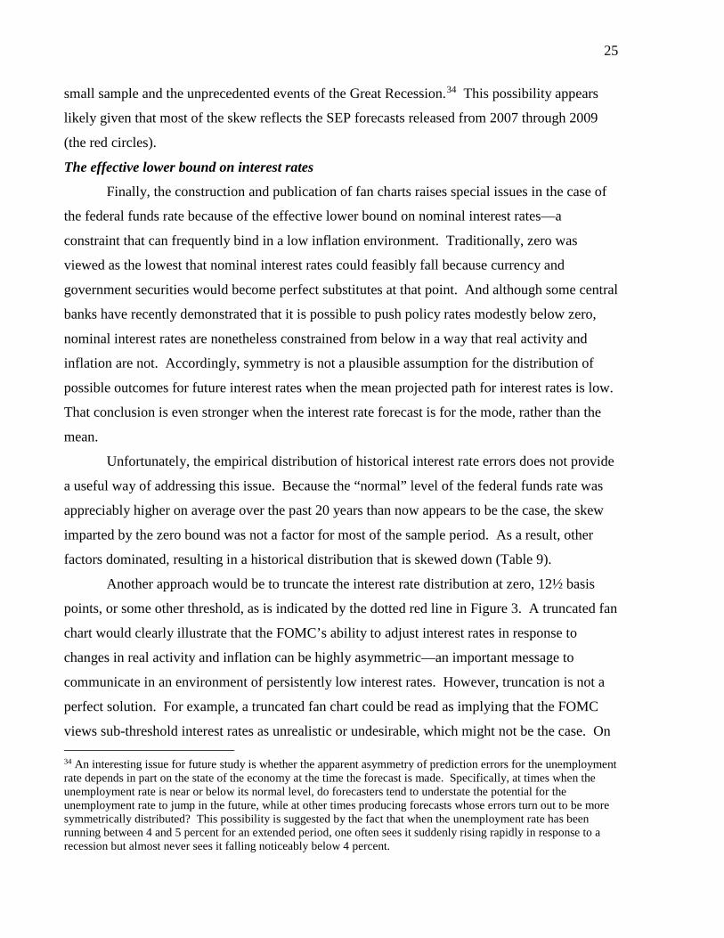
25

small sample and the unprecedented events of the Great Recession.34 This possibility appears

likely given that most of the skew reflects the SEP forecasts released from 2007 through 2009

(the red circles).

The effective lower bound on interest rates

Finally, the construction and publication of fan charts raises special issues in the case of

the federal funds rate because of the effective lower bound on nominal interest rates—a

constraint that can frequently bind in a low inflation environment. Traditionally, zero was

viewed as the lowest that nominal interest rates could feasibly fall because currency and

government securities would become perfect substitutes at that point. And although some central

banks have recently demonstrated that it is possible to push policy rates modestly below zero,

nominal interest rates are nonetheless constrained from below in a way that real activity and

inflation are not. Accordingly, symmetry is not a plausible assumption for the distribution of

possible outcomes for future interest rates when the mean projected path for interest rates is low.

That conclusion is even stronger when the interest rate forecast is for the mode, rather than the

mean.

Unfortunately, the empirical distribution of historical interest rate errors does not provide

a useful way of addressing this issue. Because the “normal” level of the federal funds rate was

appreciably higher on average over the past 20 years than now appears to be the case, the skew

imparted by the zero bound was not a factor for most of the sample period. As a result, other

factors dominated, resulting in a historical distribution that is skewed down (Table 9).

Another approach would be to truncate the interest rate distribution at zero, 12½ basis

points, or some other threshold, as is indicated by the dotted red line in Figure 3. A truncated fan

chart would clearly illustrate that the FOMC’s ability to adjust interest rates in response to

changes in real activity and inflation can be highly asymmetric—an important message to

communicate in an environment of persistently low interest rates. However, truncation is not a

perfect solution. For example, a truncated fan chart could be read as implying that the FOMC

views sub-threshold interest rates as unrealistic or undesirable, which might not be the case. On 34 An interesting issue for future study is whether the apparent asymmetry of prediction errors for the unemployment rate depends in part on the state of the economy at the time the forecast is made. Specifically, at times when the unemployment rate is near or below its normal level, do forecasters tend to understate the potential for the unemployment rate to jump in the future, while at other times producing forecasts whose errors turn out to be more symmetrically distributed? This possibility is suggested by the fact that when the unemployment rate has been running between 4 and 5 percent for an extended period, one often sees it suddenly rising rapidly in response to a recession but almost never sees it falling noticeably below 4 percent.

26

the other hand, not truncating the distribution could create its own communication problems if it

were misinterpreted as signaling that the Committee would be prepared to push interest rates into

negative territory, assuming that participants were in fact disinclined to do so. These and other

considerations related to the asymmetries associated with the lower bound on nominal interest

rates suggest that care may be needed in the presentation of fan charts to guard against the risk of

public misunderstanding.35

Conclusions

In this paper, we have presented estimates of past forecast uncertainty; these estimates are

used by FOMC participants as a benchmark against which to assess the uncertainty of the current

economic outlook. This approach, which exploits the historical forecast record of several

groups, suggests that uncertainty about the economic outlook is considerable—a point

emphasized by the Federal Open Market Committee in their communications on this issue. Our

analysis also suggests that fan charts would be a useful communication device for the FOMC to

increase public understanding about uncertainty and its policy implications.

We should repeat a caveat to our analysis: Our approach rests to a large degree on the

assumption that the past is a good guide to the future and that forecasters in the future will make

prediction errors similar to those made over the past twenty years. Although assumptions of this

sort are a practical necessity in all empirical work, we must bear in mind that estimates of

predictability have changed substantially over time. Because forecast accuracy has changed in

the past, it could change again, for better or worse. If so, error-based uncertainty estimates by

themselves could paint a somewhat misleading picture of the potential risks to the outlook.

For this and other reasons, error-based benchmarks of uncertainty and associated fan

charts are best viewed as communication tools intended to illustrate a basic point—the future is

uncertain. Attempting to go further and use this information to attempt to make explicit

estimates of the likelihood of specific events is problematic, in part because the historical

benchmarks alone do not provide a complete assessment of the uncertainty associated with the

current outlook. It is thus important that the uncertainty benchmarks discussed in this paper and 35 A truncated interval also has the drawback from a communications perspective of providing neither a one-RMSE band nor a realistic probability distribution, especially given other potential sources of asymmetry, such as those arising from the modal nature of the FOMC’s projections. Furthermore, truncation obscures how much of the probability mass for future values of the federal funds rate is piled up at the effective lower bound. While the distortion created by this pile-up problem may be relatively minor under normal circumstances, it would be significant whenever the projected path for the federal funds rate is expected to remain very low for an extended period.

27

published by the FOMC are supplemented with the qualitative assessments of uncertainty

provided by FOMC participants in the Summary of Economic Projections. Participants have at

times assessed the outlook for both real activity and inflation as more uncertain than experienced

on average in the past; they also have assessed the risks to the outlook as skewed to the

downside. This additional information helps to provide a more complete sense of possible

outcomes and risks than that obtained from participants’ individual forecasts and the benchmark

uncertainty estimates alone.

28

References Bauer, Michael D. and Glenn D. Rudebusch (2016). “Monetary Policy Expectations at the Zero

Lower Bound”, Journal of Money, Credit, and Banking, 48(7), 1439-1465. Bernanke, Ben S. (2004). “The Great Moderation,” speech delivered at the meeting of the

Eastern Economic Association, Washington (February 20), www.federalreserve.gov/boarddocs/speeches/2004/20040220/.

Bernanke, Ben S. (2007). “Federal Reserve Communications,” speech delivered at the Cato

Institute 25th Annual Monetary Conference, Washington (November 14). Brayton, Flint, Thomas Laubach, and David Reifschneider (2014). “The FRB/US Model: A

Tool for Macroeconometric Analysis,” Federal Reserve Board FEDS Notes (April), www.federalreserve.gov/econresdata/notes/feds-notes/2014/a-tool-for-macroeconomic-policy-analysis.html.

Campbell, Sean D. (2007). “Macroeconomic Volatility, Predictability, and Uncertainty in the

Great Moderation: Evidence from the Survey of Professional Forecasters,” Journal of Business and Economic Statistics, 25 (April), 191-200.

Carriero, A., Todd E. Clark, and M. Marcellino (2016). “Common Drifting Volatility in Large

Bayesian VARs,” Journal of Business and Economic Statistics, 34, 375-390. Clark, Todd E. (2011). “Real-Time Density Forecasts from BVARs with stochastic Volatility,”

Journal of Business and Economic Statistics, 29, 327-341. Croushore, Dean (2010). “Evaluation of Inflation Forecasts Using Real-Time Data,” B.E.

Journal of Macroeconomics, 10(1), Article 10. D’Agostino, A., L. Gambetti, and D. Giannone (2013). “Macroeconomic Forecasting and

Structural Change,” Journal of Applied Econometrics, 28, 82-101. Diebold, Francis X., and Roberto S. Mariano (1995). “Comparing Predictive Accuracy,”

Journal of Business and Economic Statistics, 13 (July), 253-263. Diebold, Francis X., Frank Schorfheide, and Minchul Shin (2016). “Real-Time Forecast

Evaluation of DSGE Models with Stochastic Volatility,” manuscript, University of Pennsylvania.

Engen, Eric M., Thomas Laubach, and David Reifschneider (2015). “The Macroeconomic

Effects of the Federal Reserve’s Unconventional Monetary Policies,” Finance and Economics Discussion Series 2015-005, Washington: Federal Reserve Board, www.federalreserve.gov/econresdata/feds/2015/files/2015005pap.pdf.

29

Fair, R. C. (1980). “Estimating the Expected Predictive Accuracy of Econometric Models,” International Economic Review, 21, 355-378.

Fair, R. C. (2014). “How Might a Central Bank Report Uncertainty?”, Economics: The Open-

Access, Open-Assessment E-Journal, 8 (2014-27), 1-22.

Faust, Jon and Jonathan Wright (2009). “Comparing Greenbook and Reduced Form Forecasts Using a Large Realtime Dataset,” Journal of Business and Economic Statistics, 27(4), 468-479.

Federal Reserve Board (2014). “Updated Historical Forecast Errors (4/9/2014)”,

www.federalreserve.gov/foia/files/20140409-historical-forecast-errors.pdf. Gavin, William T. and Rachel J. Mandal (2001). “Forecasting Inflation and Growth: Do Private

Forecasts Match Those of Policymakers?” Business Economics, January, 13-20. Haldane, Andrew (2012). “Tails of the Unexpected,” paper delivered at a conference sponsored

by the University of Edinburgh Business School, Edenborough (June 8), www.betterregulation.com/external/Speech%20by%20Mr%20Andrew%20Haldane%20-%20Tails%20of%20the%20unexpected.pdf.

Holston, Kathryn,, Thomas Laubach and John C. Williams “Measuring the Natural Rate of

Interest: International Trends and Determinants” Federal Reserve Bank of San Francisco Working Paper 2016-11, December 2016.

Justiniano, Alejandro and Giorgio E. Primiceri (2008). “The Time-Varying Volatility of

Macroeconomic Fluctuations,” American Economic Review, 93, 604-641. Kahneman D, P Slovic and A Tversky (eds) (1982), Judgment under Uncertainty: Heuristics and

Biases, Cambridge University Press, Cambridge. Knüppel, Malte and Guido Schultefrankenfeld (2012). “How informative are central bank

assessments of macroeconomic risks?”, International Journal of Central Banking, 8(3), 87-139.

Knüppel, Malte (2014). “Efficient Estimation of Forecast Uncertainty Based on Recent Forecast

Errors”, International Journal of Forecasting, 30(2), 257-267. Knüppel, Malte and Andreea L. Vladu (2016). “Approximating Fixed-Horizon Forecasts Using

Fixed-Event Forecasts,” Deutsche Bundesbank Discussion Paper 20/2016, Frankfurt. Mester, Loretta (2016). “Acknowledging Uncertainty,” speech delivered at the Shadow Open

Market Committee Fall Meeting, New York, New York (October 7), www.clevelandfed.org/en/newsroom-and-events/speeches/sp-20161007-acknowledging-uncertainty.aspx.

30

Mishkin, Frederic S. (2007). “Inflation Dynamics,” speech delivered at the Annual Macro Conference, Federal Reserve Bank of San Francisco, San Francisco, Calif. (March 23).

Powell, Jerome (2016). “A View from the Fed,” speech delivered at the “Understanding

Fedspeak” event cosponsored by the Hutchins Center on Fiscal and Monetary Policy at the Brookings Institution and the Center for Financial Economics at Johns Hopkins University, Washington, D.C. (November 30), www.federalreserve.gov/newsevents/speech/powell20161130a.htm.

Reifschneider, David and Peter Tulip (2007). “Gauging the Uncertainty of the Economic

Outlook from Historical Forecasting Errors,” Finance and Economics Discussion Series 2007-60, Washington: Federal Reserve Board, www.federalreserve.gov/pubs/feds/2007/200760/200760pap.pdf.

Romer, Christina D., and David H. Romer (2000). “Federal Reserve Information and the

Behavior of Interest Rates,” American Economic Review, 90 (June), 429-457. Sims, Christopher A. (2002). “The Role of Models and Probabilities in the Monetary Policy

Process,” Brookings Papers on Economic Activity, 2002 (2), 1-62. Tay, Anthony S. and Kenneth F. Wallis (2000). “Density Forecasting: A Survey,” Journal of

Forecasting, 19, 235-254. Tulip, Peter (2009) “Has the Economy Become More Predictable? Changes in Greenbook

Forecast Accuracy” Journal of Money, Credit and Banking, Vol 41, No 6 (September 2009), 1217- 1231.

Tulip, Peter and Stephanie Wallace (2012). “Estimates of Uncertainty Around the RBA’s

Forecasts” Research Discussion Paper 2012-07, Reserve Bank of Australia. Vogel, Lukas (2007). “How Do the OECD Growth Projections for the G7 Economies Perform?

A Post-Mortem”, OECD Economics Department Working Paper, No 573, Paris. Wallis, K. F. (1989). “Macroeconomic Forecasting: A Survey,” The Economic Journal, 99, 28-

61. Yellen, Janet (2016). “Designing Resilient Monetary Policy Frameworks for the Future,” a

symposium sponsored by the Federal Reserve Bank of Kansas City, Jackson Hole, Wyoming (August 26), www.federalreserve.gov/newsevents/speech/yellen20160826a.htm.

Wikipedia (2016), ‘Overconfidence Effect’. Available at

<http://en.wikipedia.org/wiki/Overconfidence_effect>, accessed November 14 2016.

31

Appendix Testing Whether Historical Forecasts are Unbiased Table 7 reports mean errors at horizons 0 to 13, using the sub-samples of forecasters reported in Table 1B. If there are N forecasters in the sub-sample at a specific horizon, the mean at that horizon is

We want to test the hypothesis that for a given horizon is equal to zero, but in doing so we should control for both serial correlation in forecasters’ errors plus the correlation of errors across forecasters. To do that, at each horizon we specify the following system of N equations:

, ,

.... , .

In this system, all forecasters are assumed to have the same bias α0. But we allow their errors to have different degrees of serial correlation (βs). Specifically, for forecast horizons from zero to three quarters, the regression includes the forecasting error at the same horizon for conditions in the previous year. For forecast horizons from four to seven quarters, the regression includes errors at the same horizon for conditions in the previous two years, errors for conditions in the previous three years for horizons from eight to eleven quarters, and errors in the previous four years for horizons greater than eleven quarters. In estimating variance-covariance matrix Ω for the error innovations, to , we allow contemporaneous innovations to be correlated across forecasters and to have different variances. The final step is to estimate this system over the sample period 1996 to 2015, and then to run a standard Wald test by reestimating the system under the restriction that α0 = 0. Testing Coverage and Symmetry To test the likelihood that the observed fraction of errors falling within plus-or-minus one RMSE at a given horizon is insignificantly different from 68 percent, we begin with the same estimated system of equations specified above, with α0 constrained to equal 0 in all cases. Under the assumption that the error innovations to are distributed normally with mean zero and the estimated historical variance-covariance Ω, we then run 10,000 Monte Carlo simulations to generate a distribution for the number of errors within a 20-year sample period that fall within the designated RMSE band. (Each simulation is run for a100 year period, and for the test we take results from the last 20 years.) The actual share observed from 1996 to 2015 is then compared to this simulated distribution to determine the likelihood of seeing a share that deviates at least this much from 68 percent, conditional on the true distribution being normal. This same Monte Carlo procedure is used to test whether the observed fraction of errors falling above the RMSE band, less the observed fraction falling below, is statistically different from zero.

32

Table 1A

Variations in Data Coverage and Reporting Basis Across Forecasters

Source

Source Release Dates Used to Compute

RMSEs for Each SEP Quarter

Horizon

Reporting Basis

Real GDP Growth

Unemployment Rate

Total CPI Inflation

Treasury Bill Rate

Federal Open Market

Committee (FOMC)

Feb (Q1 SEP), Jul (Q2 SEP)

Current year (Q1 SEP), one year ahead (Q2 SEP)

Q4/Q4 Q4 Not used Not Used

Federal Reserve

Board Staff (TB)

Mar (Q1 SEP), Jun (Q2 SEP), Sep (Q3

SEP), Dec (Q4 SEP)

One year ahead (Q1-Q2 SEP), two years ahead (Q3-

Q4 SEP)

Q4/Q4 Q4 Q4/Q4 Q4

Congressional Budget Office

(CBO)

Feb (Q1 SEP), Aug (Q2 SEP)

More than three years ahead

Q4/Q4 current and next year,

annual thereafter

Annual (not used for current and next years)

Q4/Q4 current and next year,

annual thereafter

Annual (not used for current and next years)

Administration (CEA)

Jan (Q4 SEP), May/Jun (Q1 SEP)

More than three years ahead Q4/Q4 Q4 Q4/Q4

Annual (not used for current and next years)

Blue Chip (BC)

Mar (Q1 SEP), Jun (Q2 SEP), Sep and Oct (Q3 SEP), Dec

(Q4 SEP)

More than three years ahead (Q1

SEP and Q3 SEP), one year ahead (Q2

and Q4 SEP)

Q4/Q4 current and next year,

annual thereafter

Q4 current and next year,

annual thereafter

Q4/Q4 current and next year,

annual thereafter

Q4 current and next year,

annual thereafter

Survey of Professional Forecasters

(SPF)

Feb (Q1 SEP), May (Q2 SEP), Aug (Q3 SEP), Nov (Q4 SEP)

One year ahead

Q4/Q4 current year, annual next year except for

Q4 SEP

Q4 for current year, annual

next year except for Q4 SEP

Q4/Q4 current year, annual

next year except for Q4 SEP

Q4 for current year, annual

next year except for Q4 SEP

33

Table 1B

Sources Used to Compute Errors and Related Statistics at Different Forecasting Horizons

Forecast horizon in quarters, with

publication quarter in parentheses

Real GDP Growth (Q4/Q4)

Unemployment Rate

(Q4 level)

CPI Inflation (Q4/Q4)

3-month Treasury Bill

Rate (Q4 level)

—————————— current year projections ——————————

0 (4th qtr) TB CEA BC SPF TB CEA BC SPF

TB CEA BC SPF TB BC SPF

1 (3rd qtr) TB CBO SPF TB BC SPF TB CBO BC SPF TB BC SPF

2 (2nd qtr) FOMC TB CEA BC SPF

FOMC TB CEA BC SPF

TB CEA BC SPF TB BC SPF

3 (1st qtr) FOMC TB CBO BC SPF

FOMC TB BC SPF

TB CBO BC SPF TB BC SPF

————————— one-year-ahead projections —————————

4 (4th qtr) TB CEA BC SPF TB CEA BC SPF

TB CEA BC SPF TB BC SPF

5 (3rd qtr) TB CBO BC TB BC TB CBO BC SPF TB BC

6 (2nd qtr) TB CEA BC TB CEA BC TB CEA BC SPF TB BC

7 (1st qtr) TB CBO BC TB BC TB CBO BC SPF TB BC

————————— two-year-ahead projections —————————

8 (4th qtr) TB CEA TB CEA TB CEA TB CEA

9 (3rd qtr) TB CBO1 BC TB CBO2 BC TB CBO1 BC TB CBO2 BC

10 (2nd qtr) CEA CEA CEA CEA2

11 (1st qtr) CBO1 BC1 CBO2 BC2 CBO1 BC1 CBO2 BC2

————————— three-year-ahead projections —————————

12 (4th qtr) CEA CEA CEA CEA2

13 (3rd qtr) CBO1 BC1 CBO2 BC2 CBO1 BC1 CBO2 BC2

14 (2nd qtr) CEA CEA CEA CEA2

15 (1st qtr) CBO1 BC1 CBO2 BC2 CBO1 BC1 CBO2 BC2 Note. Prior to 1989, the Federal Reserve Board staff did not report two-year-ahead forecasts of economic conditions in the September and December Greenbooks. Accordingly, forecasts from this source are not used to compute errors at horizons 7 and 8 for sample periods that begin prior to 1991. 1. Calendar year-over-year percent change. 2. Annual average.

34

Table 2

Root Mean Squared Prediction Errors for Real GDP Growth (errors in predicting actual conditions in years 1996 to 2015)

RMSEs for predictions of conditions in: Current

Year Next Year Two Years Ahead

Three Years Ahead

First-quarter projections Federal Open Market Committee 1.63 Federal Reserve Board staff 1.54 2.20 Administration Congressional Budget Office 1.69 2.15 2.141 2.181 Blue Chip 1.59 2.03 1.961 1.881 Survey of Professional Forecasters 1.63 1.871 Average 1.62 2.132 2.05 2.03 Second-quarter projections Federal Open Market Committee 1.40 2.02 Federal Reserve Board staff 1.35 2.06 Administration 1.45 2.13 2.19 2.15 Congressional Budget Office Blue Chip 1.37 1.99 Survey of Professional Forecasters 1.43 1.771 Average 1.40 2.062 2.19 2.15 Third-quarter projections Federal Open Market Committee Federal Reserve Board staff 1.19 1.93 2.18 Administration Congressional Budget Office 1.35 2.07 2.111 2.271 Blue Chip 1.23 1.89 1.971 1.931 Survey of Professional Forecasters 1.26 1.581 Average 1.26 1.962 2.05 2.10 Fourth-quarter projections Federal Open Market Committee Federal Reserve Board staff 0.79 1.75 2.24 Administration 0.88 1.84 2.16 2.19 Congressional Budget Office Blue Chip 0.89 1.68 Survey of Professional Forecasters 0.95 1.76 Average 0.88 1.75 2.20 2.19

Note. Actual real GDP is defined using the historical estimates published by the Bureau of Economic Analysis in April, 2016, adjusted for selected methodological and definitional changes to the series over time. Unless otherwise noted, growth prediction errors refer to percent changes, fourth quarter of year from fourth quarter of previous year. 1. Percent change, annual average for year relative to annual average of previous year. 2. Excludes SPF prediction errors because of non-comparability.

35

Table 3

Root Mean Squared Prediction Errors for the Unemployment Rate (errors in predicting actual conditions in years 1996 to 2015)

RMSEs for predictions of conditions in: Current

Year Next Year Two Years Ahead

Three Years Ahead

First-quarter projections Federal Open Market Committee 0.61 Federal Reserve Board staff 0.41 1.24 Administration Congressional Budget Office 0.461 1.241 1.771 1.961 Blue Chip 0.51 1.35 1.721 2.001 Survey of Professional Forecasters 0.57 1.141 Average 0.532 1.293 1.74 1.98 Second-quarter projections Federal Open Market Committee 0.37 1.24 Federal Reserve Board staff 0.36 1.22 Administration 0.40 1.28 1.80 2.01 Congressional Budget Office Blue Chip 0.39 1.27 Survey of Professional Forecasters 0.42 1.021 Average 0.39 1.264 1.80 2.01 Third-quarter projections Federal Open Market Committee Federal Reserve Board staff 0.27 1.12 1.69 Administration Congressional Budget Office 0.191 1.021 1.671 2.001 Blue Chip 0.33 1.15 1.531 1.921 Survey of Professional Forecasters 0.34 0.911 Average 0.312 1.143 1.63 1.96 Fourth-quarter projections Federal Open Market Committee Federal Reserve Board staff 0.11 0.75 1.45 Administration 0.14 0.80 1.54 1.90 Congressional Budget Office Blue Chip 0.13 0.79 Survey of Professional Forecasters 0.15 0.87 Average 0.13 0.80 1.49 1.90

Note. The actual unemployment rate is defined using the historical estimates published by the Bureau of Labor Statistics in April, 2016. Unless otherwise noted, prediction errors refer to fourth-quarter averages, in percent. 1. Annual average. 2. Excludes CBO prediction errors because of non-comparability. 3. Excludes CBO and SPF prediction errors because of non-comparability. 4. Excludes SPF prediction errors because of non-comparability.

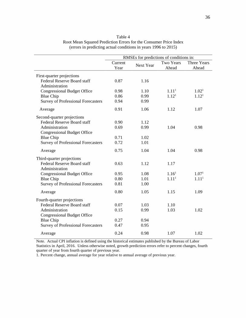
36

Table 4

Root Mean Squared Prediction Errors for the Consumer Price Index (errors in predicting actual conditions in years 1996 to 2015)

RMSEs for predictions of conditions in: Current

Year Next Year Two Years Ahead

Three Years Ahead

First-quarter projections Federal Reserve Board staff 0.87 1.16 Administration Congressional Budget Office 0.98 1.10 1.111 1.021 Blue Chip 0.86 0.99 1.121 1.121 Survey of Professional Forecasters 0.94 0.99 Average 0.91 1.06 1.12 1.07 Second-quarter projections Federal Reserve Board staff 0.90 1.12 Administration 0.69 0.99 1.04 0.98 Congressional Budget Office Blue Chip 0.71 1.02 Survey of Professional Forecasters 0.72 1.01 Average 0.75 1.04 1.04 0.98 Third-quarter projections Federal Reserve Board staff 0.63 1.12 1.17 Administration Congressional Budget Office 0.95 1.08 1.161 1.071 Blue Chip 0.80 1.01 1.111 1.111 Survey of Professional Forecasters 0.81 1.00 Average 0.80 1.05 1.15 1.09 Fourth-quarter projections Federal Reserve Board staff 0.07 1.03 1.10 Administration 0.15 0.99 1.03 1.02 Congressional Budget Office Blue Chip 0.27 0.94 Survey of Professional Forecasters 0.47 0.95 Average 0.24 0.98 1.07 1.02

Note. Actual CPI inflation is defined using the historical estimates published by the Bureau of Labor Statistics in April, 2016. Unless otherwise noted, growth prediction errors refer to percent changes, fourth quarter of year from fourth quarter of previous year. 1. Percent change, annual average for year relative to annual average of previous year.

37

Table 5

Root Mean Squared Prediction Errors for the 3-Month Treasury Bill Rate (errors in predicting actual conditions in years 1996 to 2015)

RMSEs for predictions of conditions in: Current

Year Next Year Two Years Ahead

Three Years Ahead

First-quarter projections Federal Reserve Board staff 0.84 1.94 Administration Congressional Budget Office 0.581 1.781 2.331 2.731 Blue Chip 0.92 2.09 2.491 2.861 Survey of Professional Forecasters 0.97 1.621 Average 0.912 2.023 2.41 2.80 Second-quarter projections Federal Reserve Board staff 0.68 1.90 Administration 0.221 1.481 2.221 2.671 Congressional Budget Office Blue Chip 0.74 2.00 Survey of Professional Forecasters 0.74 1.501 Average 0.722 1.953 2.22 2.67 Third-quarter projections Federal Reserve Board staff 0.41 1.64 2.31 Administration Congressional Budget Office 0.221 1.441 2.241 2.601 Blue Chip 0.58 1.74 2.091 2.661 Survey of Professional Forecasters 0.62 1.281 Average 0.542 1.693 2.21 2.63 Fourth-quarter projections Federal Reserve Board staff 0.06 1.38 2.07 Administration 0.041 0.861 1.811 2.411 Congressional Budget Office Blue Chip 0.10 1.37 Survey of Professional Forecasters 0.17 1.44 Average 0.112 1.402 1.94 2.41

Note. Unless otherwise noted, prediction errors refer to fourth-quarter averages, in percent. 1. Annual average. 2. Excludes CBO and Administration prediction errors because of non-comparability. 3. Excludes CBO, Administration, and SPF prediction errors because of non-comparability.

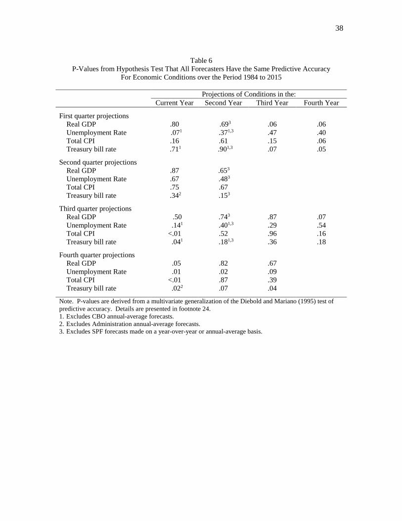
38

Table 6

P-Values from Hypothesis Test That All Forecasters Have the Same Predictive Accuracy For Economic Conditions over the Period 1984 to 2015

Projections of Conditions in the: Current Year Second Year Third Year Fourth Year First quarter projections

Real GDP .80 .693 .06 .06 Unemployment Rate .071 .371,3 .47 .40 Total CPI .16 .61 .15 .06 Treasury bill rate .711 .901,3 .07 .05 Second quarter projections Real GDP .87 .653 Unemployment Rate .67 .483 Total CPI .75 .67 Treasury bill rate .342 .153 Third quarter projections Real GDP .50 .743 .87 .07 Unemployment Rate .141 .401,3 .29 .54 Total CPI <.01 .52 .96 .16 Treasury bill rate .041 .181,3 .36 .18 Fourth quarter projections Real GDP .05 .82 .67 Unemployment Rate .01 .02 .09 Total CPI <.01 .87 .39 Treasury bill rate .022 .07 .04

Note. P-values are derived from a multivariate generalization of the Diebold and Mariano (1995) test of predictive accuracy. Details are presented in footnote 24. 1. Excludes CBO annual-average forecasts. 2. Excludes Administration annual-average forecasts. 3. Excludes SPF forecasts made on a year-over-year or annual-average basis.

39

Table 7

Mean Prediction Errors for the 1996-2015 Sample and P-Values from Wald Test that Predictions are Unbiased, by Forecast Horizon

Forecast Horizon (Quarters Ahead of Publication Date) 0 1 2 3 4 5 6 7 8 9 10 11 12 13 Real GDP growth

Mean error -0.19 -0.18 -0.34 -0.31 -0.41 -0.45 -0.71 -0.68 -0.80 -0.65 -0.90 -0.74 -0.88 -0.70 P-value 0.01 0.52 0.45 0.29 0.86 0.19 0.29 0.31 0.45 0.08 0.41 0.22 0.39 0.37 Unemployment rate Mean error -0.07 -0.08 -0.02 -0.05 -0.10 -0.04 0.07 0.07 0.05 0.05 0.26 0.11 0.27 0.21 P-value 0.01 0.11 0.26 0.29 0.24 0.89 0.63 0.86 0.86 0.56 0.68 0.73 0.50 0.70 CPI inflation Mean error -0.07 -0.19 -0.08 0.16 0.14 0.00 -0.06 -0.02 0.14 -0.04 -0.16 -0.22 -0.16 -0.28 P-value 0.42 0.01 0.47 0.61 0.67 0.57 0.51 0.51 0.98 0.84 0.44 0.49 0.48 0.48 Treasury bill rate Mean error -0.05 -0.28 -0.40 -0.42 -0.58 -0.80 -1.06 -1.08 -0.89 -1.25 -1.33 -1.65 -1.49 -1.80 P-value 0.01 0.14 0.01 0.02 0.16 0.10 0.04 0.04 0.02 0.01 0.01 0.01 0.05 0.02

Note. See Table 1B for the sub-set of forecasters whose prediction errors used to compute mean errors at each horizon. P-values are from a Wald test that the mean error at each horizon is zero, controlling for serial correlation in each forecaster’s errors, correlations in errors across forecasters, and differences across forecasters in error variances. See appendix for further details.

40

Table 8

Fraction of Prediction Errors for the 1996-2015 Sample That Fall Within Plus-or-Minus One RMSE By Forecast Horizon, And the Likelihood of Seeing an Absolute Deviation from 68 Percent as Great or Greater Assuming Normality

Forecast Horizon (Quarters Ahead of Publication Date) 0 1 2 3 4 5 6 7 8 9 10 11 12 13 Real GDP growth

Fraction 0.78 0.76 0.67 0.65 0.71 0.70 0.72 0.73 0.63 0.75 0.70 0.78 0.75 0.78 P-value 0.19 0.22 0.45 0.39 0.46 0.57 0.58 0.53 0.33 0.47 0.53 0.45 0.39 0.22 Unemployment rate Fraction 0.73 0.78 0.83 0.79 0.76 0.85 0.85 0.83 0.83 0.82 0.85 0.83 0.80 0.83 P-value 0.30 0.17 0.06 0.23 0.33 0.10 0.08 0.16 0.21 0.22 0.17 0.23 0.27 0.28 CPI inflation Fraction 0.84 0.84 0.71 0.64 0.70 0.63 0.61 0.69 0.65 0.68 0.65 0.73 0.55 0.78 P-value 0.03 0.06 0.40 0.35 0.42 0.47 0.40 0.33 0.70 0.35 0.46 0.29 0.18 0.14 Treasury bill rate Fraction 0.83 0.83 0.75 0.80 0.83 0.78 0.73 0.75 0.80 0.68 0.65 0.60 0.55 0.55 P-value 0.11 0.09 0.42 0.15 0.03 0.20 0.43 0.33 0.27 0.79 0.43 0.19 0.23 0.14

Note. See Table 1B for the sub-set of forecasters’ errors used to compute within-one-RMSE fractions at each horizon. P-values are based on the estimated distribution of errors over 20-year sample periods, derived from Monte Carlo simulations that incorporate serially-correlated forecasting errors and assume that error innovations are normally distributed with mean zero, where the serial-correlation and variance-covariance of the error innovations match that estimated for the 1996-2015 period.

41

Table 9 Symmetry of 1996-2015 Errors Falling Outside a Plus-or-Minus-One-RMSE Band by Forecast Horizon:

Fraction Above Less Fraction Below and the Likelihood of Seeing a Difference as Great or Greater Assuming Normality

Forecast Horizon (Quarters Ahead of Publication Date) 0 1 2 3 4 5 6 7 8 9 10 11 12 13 Real GDP growth

Fraction above less fraction below -0.03 -0.01 -0.03 0.01 0.01 -0.02 -0.12 -0.10 -0.13 -0.08 -0.10 -0.08 -0.15 -0.18 P-value 0.44 0.44 0.42 0.47 0.47 0.45 0.20 0.27 0.29 0.28 0.36 0.38 0.33 0.31 Unemployment rate Fraction above less fraction below -0.20 -0.05 0.01 0.06 0.04 0.15 0.15 0.08 0.08 0.08 0.15 0.03 0.10 0.13 P-value 0.06 0.36 0.45 0.32 0.38 0.13 0.11 0.27 0.26 0.26 0.18 0.45 0.23 0.19 CPI inflation Fraction above less fraction below -0.09 -0.16 -0.04 0.19 0.15 0.10 0.09 0.06 0.15 0.02 0.05 -0.07 0.05 -0.13 P-value 0.09 0.06 0.37 0.07 0.16 0.33 0.33 0.39 0.39 0.46 0.32 0.36 0.41 0.31 Treasury bill rate Fraction above less fraction below -0.17 -0.17 -0.25 -0.17 -0.17 -0.23 -0.28 -0.25 -0.20 -0.28 -0.35 -0.40 -0.45 -0.45 P-value 0.07 0.11 0.04 0.13 0.19 0.13 0.07 0.10 0.07 0.03 0.05 0.06 0.06 0.05

Note. See Table 1B for the sub-set of forecasters’ errors used to compute fraction above and fraction below a plus-or-minus-one-RMSE band at each horizon. P-values are based on the estimated distribution of errors over 20-year sample periods, derived from Monte Carlo simulations that incorporate serially-correlated forecasting errors and assume that error innovations are normally distributed with mean zero, where the serial-correlation and variance-covariance of the error innovations match that estimated for the 1996-2015 period.

42

0.6

0.8

1.0

1.2

1.4

1.6

1.8

2.0

2.2

2.4

0 1 2 3 4 5 6 7 8 9 10 11 12 13 14 15 16

1996-2015 sample period 1988-2007 sample period

Real GDP Growth (Q4/Q4)

forecast horizon in quarters

perc

enta

ge p

oint

s

0.0

0.4

0.8

1.2

1.6

2.0

2.4

0 1 2 3 4 5 6 7 8 9 10 11 12 13 14 15 16

Unemployment Rate (Q4 average)

forecast horizon in quarters

perc

enta

ge p

oint

s

0.0

0.2

0.4

0.6

0.8

1.0

1.2

0 1 2 3 4 5 6 7 8 9 10 11 12 13 14 15 16

CPI Inflation (Q4/Q4)

forecast horizon in quarters

perc

enta

ge p

oint

s

0.0

0.5

1.0

1.5

2.0

2.5

3.0

0 1 2 3 4 5 6 7 8 9 10 11 12 13 14 15 16

3-Month Treasury Bill Rate (Q4 average)

forecast horizon in quarters

perc

enta

ge p

oint

s

Source: Authors' calculations, using data published by the Bureau of Labor Statistics, the Bureau of Economic Analysis, and the Federal ReserveBoard, and forecasts made by the Federal Open Market Committee, the staff of the Federal Reserve Board, the Congressional Budget Office, theAdministration, and private forecasters as reported in the Survey of Professional Forecasters and Blue Chip Economic Indicators.

Figure 1. Benchmark Measures of Uncertainty:Historical Root Mean Squared Prediction Errors Averaged Across Forecasters

43

0.0

0.2

0.4

0.6

0.8

1.0

1.2

0 1 2 3 4 5 6 7 8 9 10

forecast horizon (quarters)

Consumer price indexPrice index for personal consumption expenditures

Inflation (Q4/Q4)percentage points

0.0

0.5

1.0

1.5

2.0

2.5

0 1 2 3 4 5 6 7 8 9 10

forecast horizon (quarters)

3-month Treasury bill rateFederal funds rate

Short-term Interest Rates (Q4 average)percentage points

Figure 2. Tealbook Root Mean Squared Prediction Errors for Different Measuresof Inflation and Short-term Interest Rates, 1996 to 2015 Sample Period

Source: Authors' calculations, using data published by the Bureau of Economic Analysisand the Federal Reserve Board, and forecasts made by the Federal Reserve Board staff.

44

-1

0

1

2

3

4

5

2011 2012 2013 2014 2015 2016 2017 2018 2019

Real GDP Growth (Q4/Q4)

2

3

4

5

6

7

8

9

2011 2012 2013 2014 2015 2016 2017 2018 2019

Unemployment Rate (Q4 average)percent

0.4

0.8

1.2

1.6

2.0

2.4

2.8

3.2

2011 2012 2013 2014 2015 2016 2017 2018 2019

PCE Inflation (Q4/Q4)

Note. Uncertainty bands equal median SEP f orecasts plus or minus av erage historical root mean squared prediction errors f or each series at the appropriatef orecast horizon. If f uture prediction errors are stable, unbiased and normally distributed, approximately 70 percent of f uture outcomes can be expected on av erage tof all within the uncertainty bands, with remaining outcomes f alling sy mmetrically abov e and below the bands.Source: Federal Reserv e Board (Summary of Economic Projections, September 2016) and authors' calculations using data published by the Bureau of Labor Statistics,the Bureau of Economic Analy sis, and the Federal Reserv e Board plus f orecasts made by the FOMC, the Federal Reserv e Board staf f , the Congressional Budget Of f ice,the Administration, and priv ate f orecasters as reported in the Surv ey of Prof essional Forecasters and Blue Chip Economic Indicators.

-1

0

1

2

3

4

5

6

2011 2012 2013 2014 2015 2016 2017 2018 2019

Federal Funds Rate (end of year)percent

Figure 3. Median September 2016 SEP Projections and Uncertainty About the Economic Outlook(shaded bands show typical range of possible outcomes based on accuracy of forecasts over the past 20 years)

percent

percent

45

-6

-4

-2

0

2

4

2.2

2.4

2.6

2.8

3.0

3.2

3.4

1985 1990 1995 2000 2005 2010 2015

current-year forecast errors (left axis) one-year-ahead forecast errors (left axis)two-year-ahead forecast errors (left axis) Blue Chip long-run projections (right axis)

Real GDP Growthpercentage points

date of outcome for errorsdate of forecast release for Blue Chip projections

-2

0

2

4

6

4.4

4.8

5.2

5.6

6.0

6.4

1985 1990 1995 2000 2005 2010 2015

Unemployment Ratepercentage points percent

date of outcome for errorsdate of forecast release for Blue Chip projections

percent

-4

-2

0

2

4

2.0

2.5

3.0

3.5

4.0

4.5

1985 1990 1995 2000 2005 2010 2015

CPI Inflationpercentage points

date of outcome for errorsdate of forecast release for Blue Chip projectionsNote. Because of confidentiality restrictions, average errors are not calculated using Tealbook forfecasts released after 2010.Source: For the forecast errors, authors calculations using data from the Bureau of Labor Statistics, the Bureau of Economic Analysis, the Federal ReserveBoard and forecasts made by the FOMC, the Federal Reserve Board staff, the Congressional Budget Office, the Administration, and private forecasters as reportedin the Survey of Professional Forecasters and Blue Chip Economic Indicators. Blue Chip long-run forecasts are taken from Blue Chip Economic Indicators.

-6

-4

-2

0

2

4

3

4

5

6

7

8

1985 1990 1995 2000 2005 2010 2015

3-Month Treasury Bill Ratepercentage points percent

date of outcome for errorsdate of forecast release for Blue Chip projections

percent

Figure 4. Blue Chip Forecasts of Long-Run Conditions and Annual Shorter-Horizon Prediction ErrorsMade by the Average of Forecasts Released in the First Quarter

46

-5

-4

-3

-2

-1

0

1

2

3

Real GDP Growth (Q4/Q4)percentage points

0 1 2 3 4 5 6 7 8 9 10 11 12 13 14forecast horizon in quarters

-3

-2

-1

0

1

2

3

4

5

6

Unemployment Rate (Q4 average)percentage points

0 1 2 3 4 5 6 7 8 9 10 11 12 13 14forecast horizon in quarters

-3

-2

-1

0

1

2

PCE Inflation (Q4/Q4)percentage points

0 1 2 3 4 5 6 7 8 9 10 11 12 13 14forecast horizon in quarters

Note. Shaded region at each forecast horizon equals plus or m inus the average root mean squared prediction error from 1996 to 2015.Source: Authors calculations, using data published by the Bureau of Labor Statistics, the Bureau of Economic Analysis, and the Federal Reserve Board, plusforecasts made by the FOMC, the Federal Reserve Board staff, the Congressional Budget Office, the Administration, and private forecasters as reported inthe Survey of Profess ional Forecasters and Blue Chip Economic Indicators.

-3

-2

-1

0

1

2

3

Federal Funds Rate (yearend)

100 percent of errors within shaded region

percentage points

0 1 2 3 4 5 6 7 8 9 10 11 12 13 14forecast horizon in quarters

72 percent of errors within shaded region 78 percent of errors within shaded region

75 percent of errors within shaded region

Figure 5. Forecast Errors for Median SEP ProjectionsReleased in 2007-2009 (filled circles) and 2010-2015 (open triangles)

(shaded region denotes typical range of errors based on average accuracy of forecasts from 1996 to 2015)