Finance and Competition∗

Harris Dellas† Ana Fernandes‡

February 18, 2013

Abstract

We investigate the role of financial constraints for product market competi-tion in a general equilibrium model, where firms may differ in terms of own wealthand/or efficiency. We find that, in general, the amelioration of financial constraintsincreases competition (it lowers the Lerner index of markups) in financially depen-dent sectors even when other standard concentration indexes indicate otherwise.Our analysis implies that disruptions in financial markets –such as the recent fi-nancial crisis– may have adverse effects on competition in product markets, a costthat has not been identified before. JEL Codes: L1, E2.

Keywords: financial constraints, liberalization, market structure, product marketcompetition, entry.

∗We are grateful to two anonymous referees as well as to the editor, Wouter den Haan, for a plethoraof valuable comments and suggestions. We want to thank to Fabrice Collard for his suggestions andhelp and also Jeff Campbell, Gerd Muehlheusser and Sergio Rebelo for helpful comments.†Department of Economics, University of Bern, Corresponding author: VWI, Schanzeneckstrasse

1, CH-3012 Bern, Switzerland. Tel: +41(0)31-631-3989, harris.dellas@vwi.unibe.ch, Homepage:http://www.harrisdellas.net/‡Department of Economics, University of Bern: ana.fernandes@vwi.unibe.ch,

http://anafernandes.name.

1 Introduction

Does the existence of financial constraints hinder product market competition in fi-

nancially dependent sectors? Do such constraints matter for the number and size of

firms as well as for concentration indexes and markups in these markets? There is a

strong presumption, based on the notion that financial constraints act as a barrier to

entry/expansion in financially dependent activities, that a more developed financial sys-

tem is conducive to greater product market competition. Surprisingly, though, there

exists no theory linking asset market development to competition. And things are not

better on the empirical front.

The empirical literature is quite meagre. Rajan and Zingales (1998), and Haber

(2000) study the effects of financial development and Cetorelli and Strahan (2006) and

Bertrand, Schoar and Thesmar (2007) the effects of changes in the degree of ”competi-

tion” in the banking sector on various measures of market structure and performance.

Rajan and Zingales find that financial development increases the number of firms while

it has an ambiguous effect on average firm size in financially dependent industries. Haber

compares the cotton industries in Brazil and Mexico during 1880-1930, a period of fi-

nancial liberalization, and argues that concentration indexes decreased, in particular in

Brazil, the country that underwent the most effective financial market reform. Cetorelli

and Strahan study how market structure in nonfinancial sectors was affected by the

increase in “competition” –lower bank concentration and looser state-level restrictions–

following deregulation in state banking in the US. They find that the number of firms

increased, average size (number of employees per establishment) and concentration de-

creased, and the share of establishments in the smallest size group also increased. Sim-

ilarly, Bertrand, Schoar and Thesmar examine the effects of lower state intervention

(deregulation) in the French banking industry on performance and competition in finan-

cially dependent sectors. They find an increase in firm entry and exit rates and also a

reduction in the level of product market concentration. .

The theoretical literature on finance and product market competition is quite ex-

tensive but, at the same time, quite narrow in scope. It has two key features. First,

it is partial equilibrium. Second, it is exclusively concerned with the strategic relation-

ship between financial decisions and output market decisions when both financial and

product markets are imperfectly competitive. One strand of the literature studies how

investors (financial intermediaries) select financial contracts or instruments in order to

1

influence the customer firm’s – as well as its rivals’ – competitive behavior: pricing deci-

sions, the incentive to enter, the incentive to collude, the choice to compete in strategic

complements vs substitutes, and so on.1 The other strand studies the reverse question,

namely, how firms select the financial contracts or instruments in order to influence the

investor’s incentives to finance other firms (whether or not to provide funds to potential

entrants, to rivals of the firms and so on2).

The objective of this paper is to provide a general framework for the study of the

relationship between financial constraints and the degree of competition in product mar-

kets. Our analysis contains four novel elements relative to the existing literature. First,

it is general equilibrium. As such, it captures the macroeconomic effects of changes

in the functioning of financial markets. Second, it allows financial markets to matter

even when they are perfectly competitive. Third, it allows for heterogeneity in efficiency

across firms. Forth, it allows for differences in the degree of financial constraints across

firms.

We employ a general equilibrium, two-sector model, with heterogeneous agents. The

agents may differ with respect to their productivity level as well as to their wealth

holdings and thus their need for external finance. One sector (sector 1) is financially

dependent in the sense that production depends on the amount of capital used and cap-

ital may need to be borrowed from the financial system.3 This sector is also imperfectly

competitive, with firms competing a la Cournot. In the other sector (sector 2), produc-

tivity is independent of capital and the market structure is perfectly competitive. There

is free entry in both sectors.

We use this model to compute the general equilibrium with and without financial

markets4 and then address the following questions. How does the amelioration of fi-

nancial constraints affect the economy’s total output and its composition, as well as

the quantity and prices of the goods produced in capital dependent sectors? How does

it affect the number and size of firms in these sectors? What is the effect on market

shares and markups? What is the role played by heterogeneity in wealth relative to

1Brander and Lewis (1986) is the pioneering work. See Cestone and White (2003) for a discussionof the literature and further references.

2See Cestone and White (2003).3In order to keep the analysis tractable, we abstract from uncertainty, agency problems and so on.

The sole role of the financial system in our model is to allocate funds from multiple savers towardinvestment projects.

4One could easily consider intermediate cases of financial market imperfections without affecting themain results.

2

that in ability? Is taking product market competition when analyzing financial frictions

important?

We find that financial markets make the output of the financially dependent sector

expand and its price drop. This is consistent with the finding of Rajan and Zingales

(1998) that industries that are more dependent on external finance grow relatively faster

in more financially developed countries. It arises from the fact that financial development

expands asymmetrically the economy’s production possibilities frontier.

The effect of the relaxation of financial constraints on the number and size of firms

as well as on market shares is ambiguous. But the effect on the degree of product

market competition (measured properly by the Lerner index) is, in general5 positive6.

These findings are important for two reasons. First, because there exists no reason to

believe that in an economy with two frictions, the elimination of one of the frictions will

in general ameliorate the other one (that is, that the effect of the frictions contains a

positive interactive term). A contribution of the present paper is to show the prevalence

–and quantitative significance– of such a positive interactive term between the financial

and the product market frictions. And second, because they establish that the standard

measures of competition commonly employed in the literature (such as the change in

the number of firms or the change in the concentration indexes) may be not be a reli-

able indicator of the change in the degree of competition in an economy with financial

imperfections.

The result that the Lerner index decreases and that this decrease represents an

improvement in competitive conditions obtains under very general parametrization of

the model. Nonetheless, the model is highly stylized, so before one accepts this result

one may need additional assurances that the model represents an empirically relevant

laboratory for the study of the question at hand. One way to address this concern is

by examining whether the model can match the stylized facts regarding net firm entry,

average firm size, and market concentration indexes reported above. Recall, that, the

literature alleges that following the amelioration of financial constrains there is positive

net firm entry, a decrease in average firm size and a decrease in market concentration

indexes. We find that the model can match this pattern under the assumption that

5While there are cases where the Lerner index may increase following the relaxation of the financialconstraints, such cases are confined to a small subset of the parameter space and are quite fragile.

6Note that even perfectly competitive firms would have a positive markup when they are constrained.Hence, a decline in the Lerner index following the removal of the financial friction does not necessarilyindicate an improvement in the degree of competition. We show that a large share of the decline in theLerner index reflects indeed an improvement in competition.

3

ability is homogeneous and the distribution of wealth in the model matches that observed

in the data. But also under a broader set of parameterizations and assumptions about

the joint cross sectional variation in ability and wealth, which is reassuring as we know

little about how these two distributions are related.

The model also has additional implications. One is that, for a given distribution of

ability and wealth and level of financial development, poorer countries will exhibit less

competitive markets that richer countries. Consequently, the gains in product market

competition arising from financial liberalization will be inversely related to a country’s

average level of income.

There are also implications regarding the political economy of financial liberalization.

A popular view is that the development of financial markets is hindered by the power

of incumbents. This includes both incumbent financial institutions that are concerned

about competition in the financial market, as well as incumbent firms that fear that

a more competitive financial system will finance entrants into their sectors. We find

that incumbency is not always sufficient to characterize preferences towards financial

liberalization. There may be incumbents who will support liberalization (efficient but

undercapitalized producers), as well as incumbents who may object to it (well capitalized

firms). It is the fact that there are situations where the financial markets tend to favor

disproportionately the most efficient but poorly capitalized producers that can account

for such divisions within the class of incumbent firms.

The paper proceeds as follows. In the next section, we present our model. Section 2

describes the model. The main results are presented in section 3.

2 The Model

2.1 The Environment

Preliminaries The economy is populated by a finite number of individuals N . In-

dividuals differ with respect to their ability level and private wealth holdings. Let Aand K denote the corresponding sets of ability and wealth. We have A = {aj}Nj=1 and

K ={kl}Nl=1

. Individual i is defined by a pair(ai, ki

)∈ A×K, i = 1, . . . , N . K denotes

the economy’s global endowment of capital, given by∑

i ki. Ability and wealth holdings

are publicly observed and common knowledge. F (a, k) denotes the joint function of

ability and wealth in the economy.

4

Production There are two goods produced in this economy. Good 1 requires capital

as an input. If individual i works in sector 1, its output qi is

qi = aikβi (1)

with β ∈ (0, 1). ki is the amount of capital individual i invests in production.

Output in sector 2 is independent of ability and, moreover, it does not require the

use of any capital. If individual i chooses to work in sector 2, he produces A units of

good 2.

In the presence of financial markets, individuals may borrow capital if their desired

scale of operations exceeds their individual capital holdings. Without financial markets,

individual investment is constrained to satisfy:

ki ≤ ki (2)

Since the ability to borrow affects the scale of individual production in sector 1 but not

in sector 2, sector 1 is said to be a financially dependent sector.

Preferences Individuals have utility defined over two goods. Given a consumption

vector (c1, c2), total utility is

u (c1, c2) = log (c1) + γ log (c2)

for γ > 0. Let p be the relative price of good 1 in terms of good 2.

Wealth endowments, kl ∈ K, are expressed in units of good 2. The income, li, of an

individual i who chooses to operate in sector 1 is:

li = ki + (pqi (ki)− ki) .

and that of one who operates in sector 2:

li = A+ ki

Individuals buy (or sell) the difference between ki and ki at the price of one.

Aggregate Demand The budget constraint for i is:

pc1i + c2

i = li

5

Given an income level li, the demand for goods 1 and 2 is:

c1i =

1

p

li1 + γ

, c2i =

γ

1 + γli

Since the Engel curves are straight lines from the origin, we have a representative agent

economy. Aggregate demand depends only on aggregate income (the sum of individual

income across individuals) and not on how it is distributed. Define

I ≡N∑i=1

li

so that I is aggregate income. Aggregate demand for good j, denoted Cj, is then

C1 =1

p

I

1 + γ, C2 =

γ

1 + γI.

The inverted demand curve for good 1 is:

p =1

C1

I

1 + γ(3)

Due to the log preference specification the (absolute value of the) elasticity of demand

of good 1 with respect to its relative price p is equal to 1. The relative demand schedule

of good 1 in terms of good 2 is:C1

C2=

1

p

1

γ(4)

Next, we examine the economy without financial constraints.

2.2 Financially Unconstrained Economy

We first describe how a firm that has chosen sector 1 selects its optimal level of produc-

tion. We then describe how firms choose their sector of activity.

2.2.1 Optimal Choice of Level of Production in Sector 1

Consider an individual i, with ability level ai. The profits from operating in sector 1

are:

π1i = p (Q1) qi − ki = p (Q1) qi −

(qiai

) 1β

(5)

where qi is the quantity produced by individual i, ki the amount of capital used, Q1 the

total output of good 1 produced, and p (Q) the inverse demand curve for good 1. We

assume that sector 1 is characterized by quantity competition a la Cournot, while sector

2 is perfectly competitive.

6

Under Cournot competition, each firm chooses output qi taking the quantities of the

remaining firms as given. The first-order condition for firm i is:

p

(1− qi

Q1

)= MC (qi) (6)

where MC (qi) indicates firm i’s marginal cost. We thus obtain the familiar result that

the price to marginal cost ratio, the markup, equals (1− qi/Q1)−1.

Equation (6) defines firm i’s optimal quantity qi in terms of the relative price p, total

market output Q1, and level of efficiency, ai. Optimal quantity qi is strictly increasing

in ability. Holding p and Q1 constant, more able firms will have greater market shares

and higher markups than less able ones. Since the marginal cost declines with ability,

more able firms are more profitable than less able ones.

Equation (6) allows us to solve for the optimal quantity produced by firm i, q∗i . It

can be written as:

q∗i = q∗i

(+p,

+

Q1,+ai

)(7)

Using the production function, equation (7) can be rewritten in terms of capital:7

k∗i = k∗i

(+p,

+

Q1,+ai

)(8)

It follows that more able firms choose a larger scale of production.

2.2.2 Optimal Choice of Sector of Activity

Individuals choose to work in the sector that generates the highest income. Let us

consider the minimum amount of capital, kmin that makes an individual of ability level

a indifferent between the two sectors. kmin(a, p) is thus determined by the equation:

paikβmin − kmin = A (9)

Equation (9) defines a relationship between ability and capital. It can be verified that

kmin(a, p) is decreasing and convex in ability. Moreover, since a higher price raises

profits for given levels of ability and capital, an increase in p shifts the kmin (·) schedule

downwards in (a, k) space.

7The strictly monotonic relationship between ability and capital depends on an additional conditionthat no firm holds a market share in excess of 50% of Q1. This will be the case if there is not a singlesuper-able agent.

7

Under appropriate assumptions on the distribution of ability and the parameters of

the model, there exists a level of ability, a, such that

kmin(p, a) = k∗(p, a, Q1) (10)

In a financially unconstrained economy, the ability level a is the threshold determining

the separation of entrepreneurs into activities: those whose ability exceeds a work in

sector 1 whereas the remaining work in sector 2. This threshold is implicitly defined by

equation (10) as a function of p and Q1:

a = a (p,Q1) (11)

(9) are depicted in Figure ??.

Once the choice of activity has been made and production completed, the aggregate

supply of good 1, Q1, is given by

Q1 =a∑

ai≥a(p,Q1)

q∗i

(+p,

+ai,

+

Q1

). (12)

Total input demand for good 1 production, K∗, is:

K∗ =a∑

ai≥a(p,Q1)

(q∗iai

) 1β

. (13)

Let Q2 denote the total quantity of good 2 produced in the economy:

Q2 =∑

ai≤a(p,Q1)

A. (14)

The quantity of good 2 available for consumption is

C2 = Q2 + K −K∗ (15)

where K is the economy’s initial endowment of capital and K∗ the amount used up in

production in sector 1.

2.2.3 The Equilibrium

Definition 1 An equilibrium in the financially unconstrained economy is a triple(a, p, {qi}Ni=1

),

with Q1 =∑N

i=1 qi, such that:

i) qi satisfies (6) for ai ≥ a and is equal to zero for ai < a;

ii) C1 = Q1, C2 = Q2 + K −K∗;iii) Equation (4) is satisfied.

8

In order to construct the equilibrium one can proceed as follows. Use (10) to solve

for a = a (p,Q1). Substituting this expression into (12), (13) and (14) yields Q1, Q2 and

K∗, respectively, as functions of p. Substituting Q1 for C1 and Q2 + K −K∗ for C2 in

(4) determines p.8

Note that in the special case of equal ability ai = a, ∀i, the equilibrium involves a

triple (n, p, q) such that: for i ≤ n, qi = q and for i < n, qi = 0; and conditions (ii)

and (iii) in the definition of the equilibrium (definition 1) are satisfied with∑

ai≥a being

replaced by i ≤ n. Hence, n identical firms operate in sector 1 and N − n identical

agents work in sector 2.

2.3 Financially constrained economy

We now discuss the determination of the equilibrium in this economy in the absence of

financial markets.9 The superscript c is used to indicate equilibrium values in the con-

strained economy. Let qci denote individual i ’s output in the constrained environment.

If this entrepreneur cannot use external funds, then his production in sector 1 cannot

exceed the level that could have been financed by his own initial capital stock, ki:

qci = min{aikβi , ai(k∗i )β} (16)

or, equivalently, in terms of capital

kci = min{ki, k∗i } (17)

where k∗i is determined by equation (8).

Unlike the financially unconstrained economy, the choice of activity now depends on

both individual ability and individual wealth. In general, it is no longer the case that

there exists a threshold ability level for the choice of activity in the financially constrained

economy, ac, or a threshold amount of capital, kcmin(a, p), such that all individuals with

ability a ≥ ac or those who have wealth exceeding k ≥ kcmin(a) will operate in sector

1. In particular, the following condition must be satisfied for individual i to operate in

sector 1:

pai(kci )β − kci ≥ A (18)

8For the cases considered in this paper, we confirm numerically that the unconstrained equilibriumexists and is unique. We do not know whether our model has this property in general. While thelog (·) preference format generates strictly convex indifference curves, the presence of Cournot imperfectcompetition may lead to segments on the production possibilities frontier with decreasing opportunitycost.

9While for reasons of simplicity we study an economy without any asset trade, our analysis isapplicable to more general environments with asset markets but with restricted asset trade.

9

Those who are not simultaneously able and rich enough to operate in sector 1, will

work in sector 2.

2.3.1 The Equilibrium

Definition 2 An equilibrium in the financially constrained economy is a set of agents

J such that:

i. For i ∈ J condition 18 is satisfied

ii. C1 = Q1, C2 = Q2 + K −Kc with Qc1 =

∑i∈J q

ci , K

c =∑

i∈J kci

iii. Equation (4) is satisfied.

3 The effects of financial markets

3.1 Measures of competition

Concentration Indexes

Let us order the firms by size so that 1 represents the largest firm, 2 the second

largest firm and so on. Then,

Definition 3 The Hj index of the market share of the j largest firms is defined as:

Hj ≡j∑i=1

qiQ1

.

Markups

Definition 4 The markup of firm i, µi is given by µi = (p−MCi)/p. When a firm is

unconstrained, its markup is determined from the first-order condition, equation (6):

µi ≡p−MCi

p=

qiQ1

(19)

And when constrained and producing suboptimal quantity q(k) by:

µi ≡p−MCi

p=p−MC

(q(k)

)p

(20)

Note that when a firm is unconstrained then the markup reflects only the imperfect

competition friction. But when it is constrained, it reflects both the imperfect compe-

tition and the imperfect capital markets friction. That is, in this case the markup is

positive even under perfect competition.

10

Definition 5 The Lerner index of monopoly, σ, is defined as

σ ≡∑i∈J

µiqiQ1

(21)

In the presence of financial constraints, a lower value of σ signifies either more com-

petition or/and a less severe financial constraint. A main focus of our paper is to assess

the interaction of the two frictions for the lerner index.

3.2 Implications for sectoral output and prices

Proposition 1 The amelioration of financial constraints leads to a lower relative price

and a higher quantity of the financially dependent good.

Proof. See the appendix.

3.3 Implications for competition, net firm entry, firm size andconcentration indexes

Having established that the amelioration of financial constraints leads to an increase in

the output and to a decrease in the price of the financially dependent sector we now

turn to the main subject of this study, namely the effects of financial constraints on

the Lerner index of competition in product markets. For the reasons offered in the

introduction, namely, a concern about the overall empirical properties of our model, we

also examine the implications of the model for entry/exit, the number and size of firms

and concentration indexes. As a means of establishing the robustness of the results

and in order to also highlight the role played by cross sectional variation in ability and

wealth, we have chosen to proceed stepwise. First we present the case where agents

are perfectly homogeneous with regard to both ability and wealth. Then we introduce

wealth heterogeneity (maintaining a common level of ability), and finally, we allow for

heterogeneity in both ability and wealth.10

3.3.1 Homogeneous ability and wealth

With identical ability, ai = a, ∀i, and initial wealth, ki = k, ∀i, all firms operating

in sector 1 produce the same level of output and have the same profits. In an interior

10The case of homogeneous wealth and heterogeneous ability is straightforward. We comment on thisbriefly below.

11

equilibrium, whether in a financially constrained economy or not, the agents must be

indifferent between the two sectors. That is, the equilibrium satisfies the condition

pakβ − k = A (22)

where k = k in the constrained economy, and k = k∗ in the unconstrained economy.

Proposition 2 For β close to unity11 (constant returns to scale), the financially un-

constrained economy has a smaller number of firms than the constrained one.

Proof. See the appendix.

Consequently, when Proposition 2holds, the lifting of financial constraints leads to net

firm exit, and to an increase to the average size of firms and concentration. Nevertheless,

markups and the Lerner index decline, as pu < pc and MCu > MCc.

We draw two conclusions from these findings. First, an increase in market concentra-

tion and/or a reduction in the number of firms does not necessarily imply a worsening

of competitive conditions (a common belief that underlies policy in this area), at least

in the presence of additional distortions (such as financial imperfections); price-cost

margins are a more reliable indicator. And second, this version of the model cannot

deliver results consistent with the empirical evidence (namely net entry and reduction

in concentration) in the absence of some sort of heterogeneity12. Furthermore, a fully

homogeneous environment produces a degenerate distribution of firm sizes, also an un-

palatable outcome. In the next subsection we examine how heterogeneity in wealth

affects the properties of the model.

3.3.2 Homogeneous ability, heterogeneous wealth

We maintain the assumption of identical ability, ai = a, ∀i but allow initial capital

holdings to vary across individuals according to the function ki = f(i). There is some

information in the literature regarding the distribution of wealth which can be used

to specify a suitable f function. We used a function that is convex in the index of

11While we can only prove analytically this proposition for β close to one, in the numerical exercisesand for all the parametrizations used in the paper we always find this to be the case, independent ofthe value of β.

12A possible and feasible extension of the model would involve examining the role played by prefer-ences for the entry-exit patterns. For, instance, using a CES instead of a log specification. We are notreporting such exercises in order not to clutter the present analysis.

12

agents that perfectly captures13 the wealth distribution in the US reported in Table 2

of Cagetti and De Nardi (2006). When solving the model14 we have used more or less

arbitrary values for the other parameters of the model (they are reported below the

Tables) but have also conducted extensive robustness analysis. The results are very

robust to alternative parameterizations.

Table I presents results for various values of aggregate wealth (initial total capital15).

As expected, the size of the financially dependent sector increases and the price of its

good drops when the financial constraint is lifted. Moreover, competition as measured

by the Lerner index always increases with the amelioration of the financial constraint

(the index declines).

Does this specification satisfy the stylized facts discussed above? The model gener-

ates net entry when the economy wide capital stock is sufficiently high16. It also has no

trouble producing a decrease in concentration indexes. It can also generate a decrease

in average firm size17 if the total stock of capital is large enough and a large fraction of

output is produced by firms that are not financially constrained.

13The results reported correspond to a specification with individuals suitably clustered at the valuesreported by Cagetti and De Nardi. Using a smoother function based on interpolation made no differencefor the results.

14The solution procedure is as follows. First, the agents are sorted in terms of their capital stock.In this case, the ordering is k1 > k2 > ... > kN . We first solve the model and compute firm profitswhen only agents 1 and 2 are in sector 1. Then we continue adding firms –in the order of their capitalstock– and solve the model with the corresponding fixed number of firms and compute profits for thefirms. The procedure stops –the optimal number of firms is reached –when a candidate firm has profitsin equilibrium that fall short of its opportunity cost in the other sector. Because initial capital ismonotonic in a suitably sorted index of agents, the procedure leads to a unique solution.

15Note that for low levels of K, the capital employed in sector 1 in the unconstrained economy islarger than the capital endowment. This can happen without at the same time undermining the biteof the financial constraint in the constrained economy if we have a static economy and we require thatagents produce with their endowment before they can go out and buy good 2. We are grateful to areferee for pointing this out.

16To be more precise: when the ratio of the aggregate capital stock to aggregate ability is high. Whenthis ratio is low, a large fraction of firms is financially constrained, in which case there is no entry inthe model. We explain this pattern below.

17In the literature, firm size is often measured by the number of employees. We measure firm size byoutput which is related to the level capital. Unfortunately, even if we were to introduce –fixed– laborin the model and interpret k as the capital-labor ratio we would still not be able to link firm size toemployment.

13

Tab

leI:

Het

erog

eneo

us

wea

lth,

hom

ogen

eous

abilit

y,C

ourn

ot

Kn

KQ

1Q

2p

σH

H(4

)si

zenc

q cW

Con

vex

wea

lth,

Con

stan

tab

ilit

y

5012

62.3

852

.90

881.

430.

090.

334.

4126

5020

40.0

035

.33

802.

551.

050.

551.

7720

1

100

1584

.46

71.0

585

1.42

0.07

10.

274.

749.

910

020

67.9

658

.02

801.

930.

497

0.49

2.90

190.

77

300

2617

3.51

143.

5174

1.40

0.04

00.

155.

522.

030

020

164.

7913

1.11

801.

640.

180

0.40

6.56

150.

50

500

3726

2.84

216.

0563

1.39

0.02

80.

115.

842.

450

020

253.

2219

3.75

801.

690.

165

0.37

9.69

150.

54

Not

e:T

he

lines

conta

inin

gb

old

chara

cter

sco

rres

pon

dto

the

econ

om

yw

ith

ou

tfi

nan

cial

con

stra

ints

.θ k

=0.

98,a

=1,β

=0.

9,A

=1,γ

=1.

Th

enu

mb

erof

agen

ts,N

isse

teq

ual

to10

0.K

=ec

on

om

y’s

end

owm

ent

of

cap

ital,n

=eq

uil

ibri

um

num

ber

of

firm

s,K

=ca

pit

alin

pu

t,Q

1=

ou

tpu

tin

sect

or

1,Q

2=

ou

tpu

tin

sect

or

2,p

=re

lati

vep

rice

,σ

=L

ern

erin

dex

,HH

(4)

=sh

are

of

4la

rges

tfi

rms,

size

=av

erage

firm

size

,nc

=nu

mb

erof

fin

anci

ally

con

stra

ined

firm

s,q c

=sh

are

of

ind

ust

ry1

ou

tpu

tp

rod

uce

dby

con

stra

ined

firm

s,W

=w

elfa

reco

nsu

mp

tion

equiv

ale

nt

of

loss

esfr

om

fin

an

cial

fric

tion

.It

isco

mp

ute

das

the

per

centa

gein

crea

sein

tota

lco

nsu

mp

tion

ofgood

1th

at

wou

ldm

ake

the

soci

ety

ind

iffer

ent

toth

eli

ftin

gof

the

fin

anci

al

con

stra

int.

14

The key to understanding the properties of the model regarding entry is in the

behavior of the incumbent firms. Table I indicates that the magnitude of net firm entry

depends negatively on the share of constrained firms. When many firms operate below

their optimal capacity (because of the financial constraint), sectoral output expansion

can take place with existing firms expanding along the intensive margin. The presence

of an operative intensive margin makes it more likely that fewer new firms will be needed

in order to meet the higher demand for good 1. Net entry is smaller and can even be

negative. Additionally, the unconstrained firms -which are larger than the constrained-

shrink with the lifting of the financial constraints (because of the decrease in the price of

good 1). The larger their share in the population, the fewer the incumbent, constrained

firms and hence the bigger the chunk of output to be produced by new firms. Convexity

in initial capital ownership works in favor of entry because it implies that the firms

that shrink are large relative to the firms that expand and also that their contraction

is large relative to the expansion of the small firms (while concavity has the opposite

implication) creating room for firm entry. Note also that the welfare gains from the

amelioration of the financial constraint as captured by the decrease of the Lerner index

depend positively on the share of constrained firms.

The Lerner index measures deviations of prices from marginal costs. But as discussed

in section 3.1, a part of these deviations is due to the financial constraint and is not

related to the existence of Cournot competition. That is, such deviations would be

present even under perfect competition18. The remaining part comes from imperfect

competition as well as from the interaction between imperfect competition and financial

constraints. A question of interest is whether this interaction matters –quantitatively

and qualitatively – for the properties of the model. In order to address this question

we solve the model under the assumption of perfect competition. Table II reports the

results. One can evaluate the importance of the interaction between the two frictions

as follows: Consider the case of K = 300. The effect of the financial friction that is

independent of the degree of imperfect competition is 0.08 (the decline in the Lerner

index following the elimination of the financial constraint under perfect competition).

The effect of imperfect competition that is independent of the financial friction (the

difference in the value of the Lerner index between imperfect and perfect competition

in the case of a zero financial friction) is 0.04. Consequently, the interaction between

18This is due to the fact that a binding financial constraint implies the existence of a non-zero markupeven under perfect competition as a competitive, constrained firm cannot adjust its quantity in orderto equate its marginal cost to the price.

15

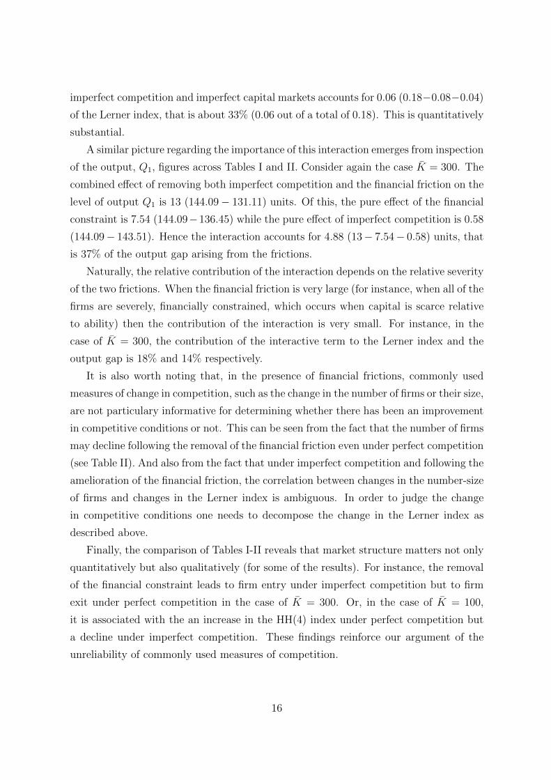
imperfect competition and imperfect capital markets accounts for 0.06 (0.18−0.08−0.04)

of the Lerner index, that is about 33% (0.06 out of a total of 0.18). This is quantitatively

substantial.

A similar picture regarding the importance of this interaction emerges from inspection

of the output, Q1, figures across Tables I and II. Consider again the case K = 300. The

combined effect of removing both imperfect competition and the financial friction on the

level of output Q1 is 13 (144.09− 131.11) units. Of this, the pure effect of the financial

constraint is 7.54 (144.09−136.45) while the pure effect of imperfect competition is 0.58

(144.09− 143.51). Hence the interaction accounts for 4.88 (13− 7.54− 0.58) units, that

is 37% of the output gap arising from the frictions.

Naturally, the relative contribution of the interaction depends on the relative severity

of the two frictions. When the financial friction is very large (for instance, when all of the

firms are severely, financially constrained, which occurs when capital is scarce relative

to ability) then the contribution of the interaction is very small. For instance, in the

case of K = 300, the contribution of the interactive term to the Lerner index and the

output gap is 18% and 14% respectively.

It is also worth noting that, in the presence of financial frictions, commonly used

measures of change in competition, such as the change in the number of firms or their size,

are not particulary informative for determining whether there has been an improvement

in competitive conditions or not. This can be seen from the fact that the number of firms

may decline following the removal of the financial friction even under perfect competition

(see Table II). And also from the fact that under imperfect competition and following the

amelioration of the financial friction, the correlation between changes in the number-size

of firms and changes in the Lerner index is ambiguous. In order to judge the change

in competitive conditions one needs to decompose the change in the Lerner index as

described above.

Finally, the comparison of Tables I-II reveals that market structure matters not only

quantitatively but also qualitatively (for some of the results). For instance, the removal

of the financial constraint leads to firm entry under imperfect competition but to firm

exit under perfect competition in the case of K = 300. Or, in the case of K = 100,

it is associated with the an increase in the HH(4) index under perfect competition but

a decline under imperfect competition. These findings reinforce our argument of the

unreliability of commonly used measures of competition.

16

Tab

leII

:H

eter

ogen

eous

wea

lth,

hom

ogen

eous

abilit

y,p

erfe

ctco

mp

etit

ion

Kn

KQ

1Q

2p

σH

H(4

)si

zenc

q cW

Con

vex

wea

lth,

Con

stan

tab

ilit

y

507

67.7

453

.98

931.

390.

000.

577.

7128

5020

4035

.33

802.

551.

050.

551.

7720

1

100

990

.47

71.8

391

1.40

0.00

0.44

7.98

8.8

100

1674

.60

60.6

884

1.80

0.33

0.60

3.79

161.

00

300

1918

0.47

144.

0981

1.39

0.00

0.21

7.58

2.2

300

2017

2.76

136.

4580

1.52

0.08

0.42

6.82

190.

88

500

3027

0.00

216.

7470

1.38

0.00

0.13

7.22

2.5

500

2026

6.72

202.

5380

1.55

0.06

0.39

10.1

315

0.52

Not

e:T

he

lines

conta

inin

gb

old

chara

cter

sco

rres

pon

dto

the

econ

om

yw

ith

ou

tfi

nan

cial

con

stra

ints

.θ k

=0.

98,a

=1,β

=0.

9,A

=1,γ

=1.

Th

enu

mb

erof

agen

ts,N

isse

teq

ual

to10

0.K

=ec

onom

y’s

end

owm

ent

of

cap

ital,n

=eq

uil

ibri

um

nu

mb

erof

firm

s,K

=ca

pit

alin

pu

t,Q

1=

outp

ut

inse

ctor

1,Q

2=

ou

tpu

tin

sect

or

2,p

=re

lati

vep

rice

,σ

=L

ern

erin

dex

,HH

(4)

=sh

are

of

4la

rges

tfi

rms,

size

=av

erage

firm

size

,nc

=nu

mb

erof

fin

anci

ally

con

stra

ined

firm

s,q c

=sh

are

of

ind

ust

ry1

ou

tpu

tp

rod

uce

dby

con

stra

ined

firm

s,W

=w

elfa

reco

nsu

mp

tion

equ

ivale

nt

of

loss

esfr

om

fin

an

cial

fric

tion

.

17

While the model with a convex function of wealth performs well under the assumption

of homogeneous ability, it is of interest to investigate the role of ability heterogeneity

for several reasons. First, entrepreneurial ability is likely to vary in the population and

its presence may undermine the success of the model obtained under homogeneity. And

second, this version of the model leads to a degenerate distribution of firm sizes which

deprives the model from additional implications. We include ability heterogeneity in the

following subsections.

3.4 Heterogeneous ability, homogeneous wealth

The results in this case are straightforward as it is the largest, most efficient firms that

face the most severe financial constraints. The relaxation of the constraint allows these

firms to expand, forcing less efficient firms to exit. Concentration and average firm size

increase, but even in this case, the Lerner concentration index declines.

3.5 Heterogeneous ability, heterogeneous wealth

We maintain the assumption of a convex function of capital holdings that satisfies the

US wealth distribution as in section 3.3.2 but now allow ability to vary across individual

according to some function ai = g(i).19

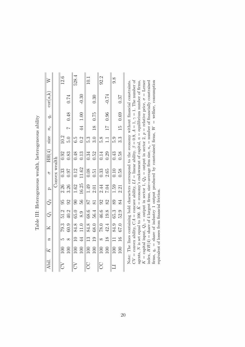
Table III reports some representative results.20 In the first four lines the ability

function g is convex in the index of agents. In the first two lines, the correlation of

wealth and ability is assumed to be positive while in the third and forth lines it is

assumed to be negative. Higher ability means a higher efficient scale of production and

thus higher demand for capital. When the correlation with wealth is positive, this higher

demand may be met through own resources so the financial constraint may or may not

be binding. Under the specification used, it turns out that most of the firms that operate

in this sector are constrained (of the 8 firms, only the largest one is not constrained).

Its lifting leads to output expansion for the constrained firms along the intensive margin

19 The evidence on the joint correlation between ability and wealth is sparse and rather inconclusive.Evans and Jovanovic (1989) find a small negative correlation between ability and wealth. Xu (1998)argues that the Evans and Jovanovic data under-represents wealth and leads to a downward bias in theestimation of that parameter. He estimates this correlation with a different data set and finds instead asmall and positive value. We take a conservative approach and experiment with different specificationsof the g (·) function. See in the appendix for the particular specifications used.

20Additional results obtained under various alternative linear and non linear specifications of abilityas well as arbitrary correlations between ability and wealth exhibit the patterns described below.

18

and output contraction for the unconstrained largest firm. The net effect is small firm

exit.

In the third and forth lines, it is the poorest that are the most able. In this case,

all the firms are constrained and the constraint is tighter relative to the previous case,

because of the negative correlation of ability and wealth. There is large expansion along

the intensive margin, with significant crowding out of firms.

In lines five through eight ability is assumed to be a concave function with either

a positive (the fifth and sixth line) or a negative correlation with wealth (the seventh

and eight line). Finally the ninth line has linear ability with a positive correlation with

wealth.

As in the case with homogeneous ability, the key consideration for determining the

entry-exit pattern is the incidence of the financial constraint over the distribution of

ability. If it is the more able that are severely constrained then the amelioration of the

constraint is likely to lead to net firm exit. If it is the less able, then the likely outcome is

net firm entry. This is due to the fact that the efficient firms have a larger optimal scale.

When their constraint is loosened, these firms expand, crowding out smaller firms as

well as potential entrants. But if they are not constrained, then the industry expansion

occurs through new entrants.

The incidence of the financial constraint over the distribution of ability and thus

the net entry-exit pattern depends both on the correlation of ability and wealth in the

population and on the –relative curvatures– of the wealth and ability functions. In

general, low variability in ability relative to that in wealth and a positive correlation

between ability and wealth make net entry more likely as they imply that the brunt of

financial constraints is felt mostly by the poorer and less efficient individuals. There is

some presumption that this is the pattern characterizing the real world.

19

Tab

leII

I:H

eter

ogen

eous

wea

lth,

het

erog

eneo

us

abilit

y

Abil.

Kn

KQ

1Q

2p

σH

H(4

)si

zenc

q cco

r(a,

k)

W

Con

vex

wea

lth

CV

100

579

.351

.295

2.26

0.33

0.92

10.2

12.6

100

860

.940

.292

3.26

0.97

0.83

5.0

70.

480.

74

CV

100

1084

.865

.090

1.62

0.12

0.48

6.5

528.

410

044

11.0

8.9

5616

.25

11.6

20.

130.

244

1.00

-0.3

0

CC

100

1384

.868

.687

1.49

0.08

0.34

5.3

10.1

100

1968

.056

.481

2.01

0.51

0.52

3.0

180.

750.

30

CC

100

878

.046

.692

2.44

0.33

0.14

5.8

92.2

100

1842

.419

.882

7.04

2.65

0.29

1.1

170.

96-0

.74

LI

100

1184

.965

.389

1.59

0.10

0.43

5.9

9.8

100

1667

.052

.984

2.21

0.58

0.58

3.3

150.

690.

37

Not

e:T

he

lin

esco

nta

inin

gb

old

chara

cter

sco

rres

pon

dto

the

econ

om

yw

ith

ou

tfi

nan

cial

con

stra

ints

.CV

=co

nvex

abil

ity,CA

=co

nca

ve

ab

ilit

y,LI

=li

nea

rab

ilit

y.β

=0.

9,A

=1,γ

=1.

Th

enu

mb

erof

agen

ts,N

isse

teq

ual

to10

0.K

=ec

on

om

y’s

end

owm

ent

of

cap

ital,n

=eq

uil

ibri

um

nu

mb

erof

firm

s,K

=ca

pit

alin

pu

t,Q

1=

outp

ut

inse

ctor

1,Q

2=

ou

tpu

tin

sect

or

2,p

=re

lati

vep

rice

,σ

=L

ern

erin

dex

,HH

(4)

=sh

are

of4

larg

est

firm

s,si

ze=

aver

age

firm

size

,nc

=nu

mb

erof

financi

all

yco

nst

rain

edfi

rms,q c

=sh

are

ofin

du

stry

1ou

tpu

tp

rod

uce

dby

const

rain

edfi

rms,W

=w

elfa

re,

con

sum

pti

on

equ

ival

ent

oflo

sses

from

fin

anci

al

fric

tion

.

20

We have also the solved the model under perfect competition for the specifications

reported in Table 3.5. With regard to the relative contribution of the interaction of the

two frictions we find basically the same results and insights as those presented in the

previous section under homogeneous ability.

3.6 Can the Lerner index increase with the amelioration of thefinancial constraint

In the specifications used so far, the Lerner index has always decreased following the ame-

lioration of the financial constraint. There are two elements that support this tendency.

The price of good 1 drops. And the level of output increases which, in a homogeneous

economy, would increase average marginal cost. But our economy is heterogeneous so it

is conceivable that the average marginal cost could move in the opposite direction, due

to relocation of production from high to low marginal cost firms. This could potentially

offset the first effect. We demonstrate this possibility below with an example.

Consider the following situation. In the constrained equilibrium, there are some large

firms that are either completely unconstrained or slightly constrained. And some smaller

firms that are more efficient than the large ones and which are severely constrained. The

latter firms have larger markups than the former because their marginal cost is lower

due to both higher ability and lower levels of production (recall that marginal cost is

increasing in the level of output). Following the amelioration of the constraint, the small,

more able firms expand and gain market share at the expense of the large firms. Their

markups decrease due to the lower price and the higher level of production. The mark

ups of the large firms may well decrease too. Nonetheless the ”average” mark up in the

economy (the Lerner index) may well increase due to the change in the market shares

of the two groups in favor of the group with the high markups.

To keep things simple, let us assume that firms are homogeneous within each of these

two groups. Let sij, i = c, u, j = H,L denote the share of industry output of firms

of type j (H indicates high and L low ability) under financial regime i ( ”c” refers to the

case with and ”u” to the case without financial frictions). And µij the corresponding

markups. The respective Lerner indexes, σc and σu are given by σc = scLµcL + scHµ

cH

and σu = suLµcL + suHµ

uH . Because µcH > µuH (and the same is likely for the L-type due

to the lower price of good 1), there is a natural predisposition for the Lerner index to

be lower in the unconstrained economy. In order to counter this propensity so that

σc < σu it is necessary that the able firms see a large increase in their output share that

21

is accompanied by a small decline in their markups21. This is theoretically possible and

the example in the Appendix demonstrates this.

While a negative relationship between the financial friction and the Lerner index can

indeed emerge, such an outcome requires, in general, finely engineered specifications of

the distributions of ability and wealth. Unlike the positive relationship obtained in the

previous sections which is very robust, the negative relationship is quite tenuous in the

sense that even slight alterations in the distribution of ability and/or wealth reverse it.

So such examples may establish the theoretical possibility of a negative relationship and

also tease out the requirements for such a relationship, but they also reveal how special

these cases may be.

3.7 Other implications of the model

The model has implications for the relationship between the level of development, the

size distribution of firms and the degree of competition in product markets. For similar

ability and wealth functions across countries the model implies that poorer countries

are likely to not only have smaller firms but also less competitive markets than richer

countries. They are thus more likely to benefit from further advancements in financial

markets.

The model can also be used to study the political economy of financial liberaliza-

tion/development. In particular, the relationship between incumbency and opposition

to liberalization? An interesting implication of our analysis is that incumbency does

not necessarily imply opposition to liberalization. For instance, in section 3.3.2 we pre-

sented cases (for instance, when all the large firms were constrained) where –at least

some– incumbents would have favored liberalization. It is also quite easy to construct

an example in which the firms operating in sector 1 do not speak with a single voice on

issues of financial liberalization.

Before concluding it is worth raising an intriguing possibility associated with the

recent disruption of the functioning of the financial markets as well as the proposed

tightening of financial regulation. To the extent that financial disruption and financial

regulation accentuate credit constraints, the degree of competition in product markets

could be an additional –and previously unidentified– casualty of the recent financial

crisis.

21The markups would not change much if the price of good 1 did not decrease significantly if themarginal cost curve were relatively flat. The larger β < 1 and ”a”, the flatter the marginal cost curve.

22

4 Conclusion

The effects of improvement in the functioning of asset markets (financial development,

liberalization, deepening...) on the allocation of resources, economic growth and welfare

have been extensively studied in the literature. There is one aspect, though, that has

received scant attention in spite of the commonly held view that it is of great importance

for economic performance and welfare. This is the relationship between finance and

competition in product markets.

In this paper we have taken a first step in characterizing the effects of financial con-

straints on competition. We have used a general equilibrium model with heterogeneity

in ability and wealth (and hence in the degree to which financial constraints may bind).

We find that the amelioration of the financial constraints in general increases compe-

tition in the product markets of the financially dependent sectors. This result is very

robust to the specification/parametrization of the model and also occurs independently

of what happens the standard market concentration indexes. Moreover, we find that the

model has good and robust overall empirical properties. In particular, it can replicate

some important stylized facts pertaining to the effects of the lifting of financial con-

straints on the distribution of firms and entry/exit patterns. Namely, it can deliver net

firm entry, a decrease in average firm size and a decrease in the standard concentration

indexes. Consequently, the model seems to represent a reliable vehicle for the study of

the relationship between finance and competition.

The analysis has been carried out in a framework that has been restricted in order

to make it feasible to study such a complicated issue. For instance, the nature of the

financial constraints has not been modelled. They correspond more closely to unspecified

costs of asset trade than to the elaborate agency problems typically discussed in the

literature; dynamics have been abstracted from; and so on. Consequently, there is

a number of demanding but important extensions awaiting.22 One could involve the

incorporation of dynamics, so that both the cross section and time series properties

of the distribution of firms in financially dependent sectors could be derived. Another

might involve making financial constraints endogenous.

22An obvious but simple extension would be to consider a more general specification for the utilityfunction in order to allow for variable expenditures.

23

References

Bertrand, Marianne , Antoinette Schoar, and David Thesmar (2007) “Banking Dereg-

ulation and Industry Structure: Evidence from the French Banking Reforms of 1985”

Journal of Finance 62(2), 597-628.

Brander, James A. and Tracy R. Lewis (1986) “Oligopoly and Financial Structure: The

Limited Liability Effect” American Economic Review 76(5), 956-970.

Cagetti, Marco and Mariacristina De Nardi (2006), ”Entrepreneurship, Frictions and

Wealth,” Journal of Political Economy 114(5), 835–870.

Cestone, Giacinta and Lucy White (2003) “Anticompetitive Financial Contracting: The

Design of Financial Claims” Journal of Finance 58(5), 2109-2142.

Cetorelli, Nicola and Philip Strahan (2006) “Finance as a Barrier to Entry: Bank Compe-

tition and Industry Structure in Local U.S. Market ” Journal of Finance 61(1), 437-461.

Evans, David S. and Boyan Jovanovic (1989) “An Estimated Model of Entrepreneurial

Choice under Liquidity Constraints” Journal of Political Economy 97(4), 808-827.

Glen Jack, Lee K. and Ajit Singh (2004) “Corporate Profitability and the dynamics

of Competition in Emerging Markets: A Time Series Analysis”, Economic Journal

113(491), F465-F484.

Haber, Stephen (2000) “Banks, Financial Markets, and Industrial Development: Lessons

from the Economic Histories of Brazil and Mexico” Center for Research on Economic

Development and Policy Reform Working Paper 79.

Levine, Ross (2005) “Finance and Growth: Theory and Evidence” in Handbook of Eco-

nomic Growth, Philippe Aghion & Steven Durlauf (eds.), (North-Holland) Vol. 1, Part

1, 865-934.

Rajan, Raghuram G. and Luigi Zingales (2003) “The Great Reversals: the Politics

of Financial Development in the Twentieth Century” Journal of Financial Economics

69(1), 5-50.

Tybout James (2000) “Manufacturing firms in developing countries: How well do they

do and why?” Journal of Economic Literature 38(1), 11-44.

24

Xu, Bin (1998) “A re-estimation of the Evans–Jovanovic entrepreneurial choice model”

Economic Letters 58(1), 91-95.

25

5 Appendix

Proposition 1: The financially unconstrained economy has a lower relative price and

a higher quantity of the financially dependent good.

Proof. Let us remove the financial constraints and hold p fixed. Borrowed capital now

allows the –previously– financially constrained firms to expand output. The output of

the financially unconstrained firms (if there are any) will also increase due to equation

(6). Hence, C1 is higher. The increased use of good 1 as capital in sector 1 implies

a lower level of C2. Consequently, the production of good 1 relative to that of good

2 increases as well. Compared to the equilibrium prevailing before the removal of the

financial constraints, there is now an excess supply of good 1 relative to that of good 2.

In order for equilibrium to be restored p must decrease.

Could Q1 end up being lower in the unconstrained equilibrium? Given that a lower

p requires C1/C2 to increase, this would require a decrease in C2. But C2 can decrease

only if either more of good 2 is used as capital in sector 1 or (and) if fewer agents operate

in sector 2. In either case, that implies a higher C1(Q1). �

Proposition 2: Under homogeneous ability and wealth, the financially unconstrained

economy has a smaller number of firms than the constrained one when β is close to one.

Proof. Let N be the total number of agents and n the number of firms in sector 1.

Equation (4) can be re-written as γpC1 = C2 = (N − n)A+ K − nk. Multiplying both

sides of (22) by n and substituting for nk in the previous expression leads to

pC1 =NA+ K

1 + γ

Consequently, pC1 and C2 are independent of the existence of financial constraints.

Hence,

pC1 = pcqcnC = pca(kc)βnc = pua(ku)βnu = puqunc

Let β = 1. We then have that nc > nu iff pckc < puku.

From equation (22) we have

A = apckc − kc = apuku − ku

Equation 5 can be rewritten as a(pckc−puku) = kc−ku, which implies that pckc < puku)

iff kc < ku. But equation 5 can also be written as (apc−1)kc = (apu−1)ku which implies

that kc < ku iff pc > pu. Hence, nc > nu.

26

Figure 1: Ability and initial capital holdings

0

0.2

0.4

0.6

0.8

1

1.2

0 5 10 15 20 25 30 35

a

k

Ability and initial capital holdings

cv+ cv- cc+ cc-

CV signifies convex and CC concave ability. A ’+’ signifiespositive correlation of ability with wealth and a ’-’ a negativecorrelation.

27

Negative correlation between the friction and the Lerner index

Table IV: Negative correlation between the friction and the Lerner index

K n K Q1 Q2 p σ HH(4) size nc qc cor(a,k) W

37 3 15.92 32.18 7 0.87 0.644 1 10.73 2537 4 15.79 26.60 6 1.02 0.627 1 6.65 1 0.11 0.38

Note: The first row corresponds to the economy without financial constraints. β = 0.9, A = 1, γ = 1.The number of agents, N is set equal to 10. For variable definitions see the notes to the previous tables

Table V: Initial wealth and ability

Agent 1 2 3 4 5 6 7 8 9 10ki 10 10 10 1 1 1 1 1 1 1ai 2 2 1.5 1 1 1 1 1 1 3

N=10, Correlation(ki, ai) = 0.38. Note: The negative relationship between the friction and σ obtainedin this example is very fragile. For instance, changing agent 9’s level of ability from 1 to 3 overturnsthe negative correlation (σc = 0.92, σu = 0.48).

28

Table VI: Properties of the equilibrium

Agent 1 2 3 10Constrained

qi 9.43 9.43 4.72 3dC/dqi 0.66 0.66 0.84 0.37qi/Q 0.35 0.35 0.18 0.12µi 0.55 0.55 0.21 1.76

Unconstrainedqi 8.21 8.21 15.75

dC/dqi 0.65 0.65 0.44qi/Q 0.26 0.26 0.48µi 0.34 0.34 0.96

29