maNASA-CR-199942

Final Report: PARALLELIZED MODELLING ANDS O L U T I O N S C H E M E F O RH I E R A R C H I C A L L Y SCALEDSIMULATIONS NAG-31142

Joe Padovan

The University of Akron

Akron, Ohio 44325-3903

(Akron Univ.) 95 p

N96-16265

Unclas

G3/62 0086502

https://ntrs.nasa.gov/search.jsp?R=19960009099 2018-06-24T15:07:14+00:00Z

Final Report: PARALLELIZED MODELLING ANDS O L U T I O N S C H E M E F O RH I E R A R C H I C A L L Y SCALEDSIMULATIONS NAG-31142

Joe Padovan

The University of Akron

Akron, Ohio 44325-3903

Index x

Section Page

1) Part I

1-i) Abstract 1-i

1-1) Introduction 1-1

1.2) The General HPT Methodology 1-4

1.3) Edge-Bisection 1-13

1.4) Interpolative Reduction Methodology 1-17

1.5) Hybrid Methods 1-24

1.6) References 1-31

Appendix Part 1 1-34

Figure Legends - 1-37

Figures 38-

2) Part II

2.i) Abstract 2-i

2.1) Introduction 2.1

2.2) FE/FD Models 2.2

2.3) Applications of the HPT Scheme 2.5

2.4) Benchmark Applications 2.11

2.5) References 2.18

Figure Legends 2.21

Figures 2.22-

Hierarchically Partitioned Solution Strategy ForCFD Applications: Part I - Theory

Joe PadovanA

Departments of Mechanical and Polymer EngineeringThe University of AkronAkron, Ohio 44325-3903

1- i

Abstract

This two-part paper presents the results of a benchmarked analytical-numerical

investigation into the operational characteristics of a unified parallel processing strategy for

implicit fluid mechanics formulations. This Hierarchical Poly Tree (HPT) strategy is based

on multilevel substructural decomposition. The Tree morphology is chosen to minimize

memory, communications and computational effort. The methodology is general enough to

apply to existing finite difference (FD), finite element (FEM), finite volume (FV) or spectral

element (SE) based computer programs without an extensive rewrite of code. In addition

to finding large reductions in memory, communications, and computational effort associated

with a parallel computing environment, substantial reductions are generated in the sequential

mode of application. Such improvements grow with increasing problem size. Along with

a theoretical development of general 2-D and 3-D HPT, several techniques for expanding the

problem size that the current generation of computers are capable of solving, are presented

and discussed. Among these techniques are several interpolative reduction methods. It was

found that by combining several of these techniques that a relatively small interpolative

reduction resulted in substantial performance gains. Several other unique features/benefits

are discussed in this paper. Along with Part I's theoretical development, Part II presents a

numerical approach to the HPT along with four prototype CFD applications. These demon-

strate the potential of the HPT strategy.

1-1

1 Introduction

The anticipated capacity of supercomputers of the near future falls orders of magnitude short

of meeting the demands of Computational Continuum Mechanics (CCM). Weather predic-

tion, combustion modeling, full field aerodynamic simulations, fluid-structure interaction

models, among others, are hampered by inadequate computational speed and memory

capacity. Limited computer capacities of the past, have fostered the use of explicit methods

to maximize the size of the models solved. Their success is due to the facts that they are

easy to program, require a minimum of storage, and run fast for simple models that are

based on a restrictive set of assumptions. However, as modeling progresses, their weak-

nesses have surfaced. As the restrictions relax, the resultant set of discretized nonlinear

ODEs stiffens. Very small time steps are required for stability. This has sparked a sub-

stantial amount of research into the application of implicit methods to Computational Fluid

Dynamics (CFD) models [1,2]. Implicit methods require matrix inversion. This inversion

can be accomplished in three ways, direct matrix inversion, iteration, or by hybrid

methods [3]. Iterative techniques require a minimum of memory. For small matrices, i.e.

small models, iterative processes converge quickly, and are faster than direct inversion.

However, for the class of CFD problems, large nonlinear sparse, unsymmetric systems,

iterative methods are not guaranteed to converge [4]. Furthermore, as the problem size

grows, their convergence rate deteriorates to the point that they may become less efficient

than direct matrix methods. Iterative methods seem to be popular with researchers, but not

with end users who seem are not willing to tolerate the lack of convergence or cannot afford

the associated computer costs. In another arena of CCM, Solid Mechanics, the issue of

direct matrix inversion versus other inversion techniques, has been settled in the commercial

1- 2

market place. Virtually all commercially successful, general purpose, solids analysis codes,

e.g. NASTRAN, ABAQUS, ADINA, etc., are based on direct matrix inversion (via a variant

of Gaussian elimination). In this vein minimization of the effort associated with the direct

matrix inversion process is sought.

Previous works by the authors, et.al., have provided lower bound approximations to

computational effort and memory requirements associated with the sequential and parallel

application of the concept of Hierarchical Poly Trees (HPT) to a broad class of CCM formu-

lations [5-9]. This includes heat transfer and solid mechanics. Linear and nonlinear as well

as steady state and transient aspects have been treated. Additionally, the HPT can be

employed at the modeling stage, i.e. a preprocessor capable of taking advantage of, and

aiding, modeling tasks such as geometric cell cloning, a feature associated mesh enrichment

(FAME) [10] etc. Briefly stated, HPT implements multilevel substructural decomposition

to achieve reductions in memory, computational effort, and communication requirements.

HPT methodology shows increasing computer effectiveness in terms of both memory and

computational effort. HPT methodology extends this sequential performance improvement

to the parallel processing environment in such a natural way that system overhead is mini-

mized. The HPT methodology is general enough to be applied to existing FD/FV/FEM/SE

codes without an extensive rewriting of code and can be implemented on existing parallel

computer architectures. Note that the HPT substructural decomposition does not require

iteration as do some other domain decomposition techniques such as the subdomain patching

methods [11] based on the Schwartz Alternating Scheme (circa 1860's).

In this two-part paper, the authors present the results of research on two and three

dimensional fluid formulations employing the Hierarchical Poly Tree (HPT). Along with

1- 3

a formal analytical-numerical development, the resulting implications in the area of parallel

computer processing are presented. This includes the results of several benchmark computa-

tional fluid dynamics (CFD) applications.

The main objectives are to i) minimize inversion effort, ii) reduce memory utilization

and, iii) limit the communications burden. As will be seen, this can be achieved through the

use of the HPT concept. Specifically, what is needed is a reduction in the bandwidths

associated with model connectivity. While global minimizers [12] such as those of Cuthill-

McKee [13] and Gibbs-Poole-Stockmeyer [14] yield significant improvements, since they are

geared primarily to global bandwidth reduction, local characteristics cannot be exploited.

As a result, globally minimized models generally consist of thinly populated diagonal and

skyline regions. In between these zones is significant numbers of zeros, i.e. Fig. (1). These

of course burden the direct inversion process. A remedy to this situation, is to affect the

removal of the zeros between the skyline and diagonal matrix regions.

Part I will overview the major features of the HPT as applied and specialized to 2-D

and 3-D CFD simulations pertaining to either symmetric or unsymmetric systems of equa-

tions. Special emphasis will be given to describe bounds on performance characteristics for

simplified geometries. In this context the sections will 1) describe the scheme, ii) develop

analytical procedures to optimize the model dependent HPT, and iii) overview potential

speedup/memory and communications reductions for simple geometries.

Part II extends the scheme to more general geometries via a numerical scheme.

Additionally, comprehensive CFD example problems are presented along with their HPT

speed ups.

2 The General HPT Methodology

The HPT concept is employed to compress the bandwidth. This is achieved by hierarchically

partitioning the model into multilevel substructures. The central focus of the scheme is to

eliminate the internal degrees of freedom of each of the various partitions (cells) at every

level of the tree. Note, the substructure at the top of the tree generally have narrower band-

width profiles. This is a direct result of the smallness of the partitions. To maintain the

advantage of bandwidth compactness, the partitions chosen at each level must be such that

an optimal balance is achieved between the internal and external degrees of freedom. In

particular, since the tree requires multiple subassembly steps at each of the various branch

levels, the balance between internal and external degrees of freedom must be such that band-

width compactness is maintained at each and every level. Once this is achieved, a significant

number of zeros can be squeezed out of the effort, memory, and communications burden.

There are difficulties associated with the foregoing process. These consist of i) the fact

that substructuring intrinsically expands the bandwidth of local partitions, ii) the choice of

the proper partition shape is problem dependent and iii) the number of partitions and levels

must be determined. The first of these, bandwidth expansion, is a direct outgrowth of the

internal-external segregation process central to substructuring, refer to Fig. (2). Recall that

the partition level equations take the form

(K]{Y} = {F} (1)

The optimal connectivity necessary to minimize the bandwidth of [K] requires an intermixing

of internal and boundary nodes. Once substructuring is introduced, (1) is partitioned as

follows,

This process significantly expands the bandwidth, Fig. (2). For example, given an (N,N,N)

cubic region, typically the optimal bandwidth is 0(W2). The external-internal partitioning

process can expand the mean half bandwidth to O(6Af2) for intermediate level partitions. To

overcome the work effort expansion, care must be taken to balance the ratio of internal to

external variables in each succeeding branch level. As would be expected, such balancing

is intimately tied to the choice of partition shape, the number of branches per level as well

as the number of total levels.

2.1 Formulation

For the purpose of developing upper bound analytic estimates of computational effort,

memory requirements and communications burden, assume that the cell is a 3-D cube. To

balance the tree, decompose the cell into partitions which yield the minimum external/

internal ratios, Fig. (3). This is achieved for cubic zone shapes.

To establish the zone sides and number of levels, the Gaussian elimination process is

relied on to determine the operations count. Since the forward matrix reduction phase

requires the major effort, it is used to structure the tree architecture. Since cubic regions

have an essentially regular node connectivity, the forward effort count (multiply-division-

addition pair) takes the form [15]

Fe = Ne(BW)2 (3)

such that Ne defines the number of equations and BW is the associated mean half bandwidth.

Based on the HPT tree structure the number of branches associated with each succeeding

level are given by the tuple

After determining the node connectivity and skyline associated with either a FD grid or finite

element model, replace the mean-half-bandwidth with the skyline height in equation (3). The

resulting effort for an unsymmetric skylined system can be shown to be the sum of the sky-

line heights (S^) squared,

Fe = £ S? (4)1=1

Memory for the system is then simply the sum of the skyline heights. For discussion

purposes the effective mean half bandwidth (5W). is determined. To do this, the effects of

substructuring induced bandwidth expansion must be taken into account at every branch

level.

2.1.1 2-D Formulation

In 2-D the Kt tuple defines k( dissections per edge of the (z'-l)th substructure, i.e.,

*, = *; i c [2, /]

After much symbolic algebra type bookkeeping, it can be shown that, for square zones

defined by either 5 noded FD or 4 noded FE models,

(5W), * 3 p N, (6)

(BW). « 3.75 p Nt; i e [2, I - 1] (7)

(BW\ « 1.75 p N (8)

where the associated population counts take the form

(Mr), - p(N,y (9)

(Ate), - 2 p(kM + 1) N.; i e [2, 7 - 1] (10)

1-7

(Ne\ » 2 P(k2 + 1) N (11)

N. = 1 + (N - l)/n*,; i e [2, 7] (12)

such that p is the number of degrees of freedom per node and N is the number of nodes per

edge. Employing (6-12), the net effort, memory and communications burden can be cast in

the following form for sequential type applications.

1) Effort

/=2

Fe = (Fe)f (13);=i

(Fe), - 9

(Fe)f « 28.1 P3(*M + 1) (M)3 n^; i e [2, 7 - 1] (15)

\;=2 '

(Fe}, - 6.12 P\k2 + 1) (yV)3 (16)

2) Memory

/Me = ^ (Me),. (17)

1=1

(18)

- 15 p2^,,, + 1) (yV,)2 (j][A',)2; / e [2, 7 - 1] (19)\/ = 2 '

(Me), » 7 p2()t2 + 1) (//)2 (20)

3) Communications

Ce = E (Ce), (2Di = 2

(Cc)f = 16 p2(A',.)2 (;V.)2 (n/rj2; i e [2, 7] (22)

1- 8

Here Me and Ce denote the memory and communications burdens. Note the communi-

cations requirements are a result of the transfer of the reduced substructural stiffness matrix

associated with the external degrees of freedom.

2.1.2 3-D Formulation

In 3-D, the Kt tuple defines kf dissections per edge of the (z-l)th substructure, i.e.,

*, = (K,.)1'3; i e [2, /] (23)

After much bookkeeping and the aid of some symbolic algebra, it can be shown that, for

cubic zones of either 7 noded FD or 8 noded FE models,

(BW), « 4 p N2 (24)

(BW)t » 6 p N2; i e [2, I - 1] (25)

(BW\ » 3 p N2 (26)

where the associated population counts (number of equations) for the HPT take the form

(Ne), » P(N,}3 (27)

(to), - 3 P(kM ••• 1) N?; i e [2, I - 1] (28)

(Ne\ » 3 p(k2 + 1) N2 (29)

N,= I + ( N - l)/n*,; »e V> ^ (30)

1=2

such that p is the number of degrees of freedom per node and N is the number of nodes per

edge. Employing (24-30), the net effort, memory and communications burden can be cast

in the following form for sequential type 3D applications.

1) Effort

Fe =

1=1

1- 9

(Fe), - 16pW(lI*iF (32)\ /=2 /

(Fe), - 108 P3(*M + 1) (AT.)6 (ri*,)3; i e [2 , I - 1] (33)

\;=2 '

(Fe\ - 27 p3(£2 + 1) (#)6 (34)

2) Memory

/(35)

(36)

(Me),. » 36 p2(^,.+1 + 1) (NJ* (n^)3; i e [2, 7 - 1] (37)\;=2 '

(Me\ » 18 p2(/:2 + 1) (N)4 (38)

3) Communications

(Ce)f (39)

(00, - 36p2(^,.)4(n^)3; ie [2,7] (40)\;=2 '

By proper balancing, Fe, Me, and Ce can be optimized.

2.1.3 Optimization of the HPT Method

Noting the structure of (13-22 and 31-40), it follows that % and N{ are nonlinearly coupled

throughout the formulation. To obtain an optimal solution, several approaches can be

utilized namely, we can minimize Fe, Me or Ce separately or in Lagrange multiplier coupled

groups [16]. For the multiplier approach, the criterion function is given by the expression

0 = Fe* + x Me* + z Ce* (41)

i = 2

where effort, memory and communications have been rewritten to conform to the method

of Lagrange Multipliers as

/Fe*(N(, *,) = Fe - £ (F«), (42)

1=1/

Me*(Nf, k.) = Me - £ (Me). (43)1=1

Ce*(#, *) = Ce - ( C e ) (44)i=2

Now treating the real world memory limitations and communications burden of a typical

computer system as mathematical constraints in the optimization process, we yield the

following system.

= 0 i e [2, /] (45)

T = ° z' e [2' /] (46)a*.

subject to the constraints

Me* = 0 and (47)

Ce* = 0. (4g)

Overall (45-48) represent 21 nonlinear equations. Note they provide a linearly weighted

optimization of effort, memory and communications burden. Many alternative formulations

are possible. To a great extent, the appropriate choice requires specific hardware specifica-

tions, i.e. CPU speed, memory capacity, bus transfer speeds, the number of i/o channels,

etc.

1- 11

2.2 Asymptotic Results

For the purpose of obtaining asymptotic expressions for speedup and memory reduction,

computational effort will be minimized. This yields the following optimality criteria namely,

^ = 0; i e [2, 7] (49)dk,

Similar equations apply for the optimization of Me or Ce.

2.2.1 Asymptotic 2-D Results

Employing (49), the optimal two level tree structure for the square cell is given by the

relation

k ~

where here k denotes the number of second (top) level branches for a sequentially processed

flow of calculations. The associated speedup relative to the global application of LU

decomposition takes the form

S ~

such that S denotes the speedup. For the effort optimized tree, the memory reduction takes

the form

M ~ 0Ar"3 (52)

As can be seen from (51 and 52), order of magnitude improvements are afforded by the HPT

scheme as the problem size grows. These conveniently apply simultaneously to speedup,

memory as well as for communications. Similar but more complex relations can be derived

for problems involving several branch levels. The various trends will be discussed later.

1-12

2.2.2 Asymptotic 3-D Results

Similarly, the optimal two level tree structure for the cubic cell is given by the relation

k ~ 0(NIIS) (53)

where here k denotes the number of second (top) level branches for a sequentially processed

flow of calculations. The associated speedup relative to the global application of LU

decomposition takes the form

5 ~ 0(N4'5) (54)

such that S denotes the speedup. For the effort optimized tree, the memory reduction takes

the form

Mr ~ 0(N'2IS) (55)

2.3 Discussion/Comparison with 2-D Results

The bandwidth associated with the 2-D HPT is of the order 0(N); whereas, the bandwidth

associated with the 3-D Tree is O(N2). Thus the later (3-D) is more sensitive to conservative

estimates of bandwidth. Since the effort is proportional to the bandwidth squared and

memory is proportional to the bandwidth, effort is most affected. Although the analytic

expressions have been developed for cubic morphologies, thin 3-D sections can be treated

similarly to 2-D for estimations of effort, memory and communications burden, provided that

the nodes in the thin direction are accounted for. If the region is somewhat between a thin

3-D shape and a cubic morphology then the speedup and memory reductions will range

between those of the 2-D and 3-D HPT. Asymptotic orders of magnitude of improvements

associated with 2-D HPTs are well within current computer capacities. But the asymptotic

orders of magnitude of 3-D improvements are beyond current computer capacities. In other

1- 13

^^ words, even though the 3-D HPT has a larger potential for improvement, considering the

capacity of current generation computers, exploiting this potential is a challenge. Therefore

the next sections present strategies to bring these improvements to current problem size.

2.4 HPT Strategy for Sequential Improvement

As the number of partitions increase, the limiting factor to the increase of speedup and

memory reduction is the accumulating root burden. After a point this root burden tends to

negate any advantage gained in the upper levels of the tree by increasing the number of

partitions. Unfortunately, the root burden dominates early in the 3-D HPT. There are two

methods that can eliminate some of the root burden.

• Edge Bisection.

• External Elimination.

These methods will be considered in the following section.

3 Edge-bisection

As pointed out earlier, the accumulation of burden at the root of the Tree, tends to blunt the

potential of the 3-D HPT. Earlier work with the 2-D HPT has shown that edge bisection can

be effective in the reduction of root burden. This is accomplished as a transfer of some of

the root burden to the upper levels of the tree. Edge-bisection means that each successive

level in the tree is partitioned in such a way that a 3-D solid would split into eight sections,

zones, cells or partitions. That is;

k. = 2; i e [2, /] (56)

1- 14

For example the second level in the 3-D Tree is composed of 8 cells. The third level is

composed of 8x8 or 64 cells, and so forth. Refer to Fig. (3) for an illustration of the

multilevel Edge-bisection process.

3.1 Formulation

In a manner similar to that of the expressions for the general 3-D case the mean half band-

width, net effort, memory and communications burden can be cast in the following form for

sequential type applications.

(BW), = 4 p[l + (N - l)/(2/-1)]2 (57)

(BW). » 6 p[l + (N - l)/^1'-1)]2; i e [2, I - 1] (58)

(5W), - 3 PN2 (59)

where the associated population counts take the form

(MO, = p[l + (N - l)/(2'-l)-\3 (60)

(Ne\ » 9 p[l + (N - l)/(2/-1)]2; i e [2, 7 - 1] (61)

(MO, « 9 p^V2 (62)

1=1

N, = 1 + (N - l)/(2''1); » e [2, 7] (64)

1) Effort

Fe (65)

(Fe), * 16 p3[l + (tf - l)/(2/'1)]7 [23(/-1)] (66)

(Fe). = 324 P3[l + (N - l)/(2'-1)]6 [23(i^]; i e [2, I - 1] (67)

(Fe), « 81 p\N)6 (68)

x~ 15

2) Memory

/Me = £ (Me),. (69)

1=1

(Me), = 8 p2[l + (N - l)/(2/-1)]5 [23{/-1)] (70)

(Me). = 108 p2[l + (N - l)/(2'-1)]4 [23('-»]; I e [2, 7 - 1] (71)

(Me), » 54 p2(#)4 . (72)

3) Communications

Ce = £ (Ce)(. (73)i=2

(Ce),. - 288 p2[l + (W - l)/(2'-')]4 [23(M)]; i e [2, I] (74)

The Edge-bisection method (EBHPT) yields substantial improvements by increasing the

number of levels in the tree rather than increasing the number of partitions; however, the

^^ full potential of this method has not yet been fully exploited. The next subsection discusses

a process of reducing and/or eliminating external boundary nodes, which in combination with

Edge-bisection will provide even greater improvements.

3.2 External-elimination and Edge-bisection

Early removal (at or near the top level) of external boundary nodes from the HPT process

can improve performance characteristics. All of these external boundary nodes can be

removed at the top level of the tree by any combination of the following two techniques.

• Substructural decomposition/condensation/reduction.

• Assembly.

Treat the external boundary nodes as internals and use substructural decomposition to

condense/reduce them from the HPT at the top level. The associated cost is negligible

1-16

compared to the overall internal/external reduction process at the top of the tree. Many

simulations/models have large portions of their boundaries predetermined (fixed boundary

conditions). Fluid simulations are a particular example. In this instance, external boundary

nodes are removed at assembly with no appreciable cost to the process. So far the analytic

expressions have, been based on the effort of interior cells or cells that have not had their

externals reduced or eliminated. This leads to over estimation of the effort, memory and

communications burden. The Edge-bisected 3-D HPT is particularly sensitive to this, since

the root and lower levels are primarily composed of external cells. Modifications to reflect

the influence of external cells with their external surface nodes reduced/eliminated, yield

expressions for effort, memory and communications burden, where the associated cell

population counts take the form.

(A^), = 1 (75)

(tf4J), = 3C2'-1 - 1) (76)

(N5s)t = 3(2" - I)2 (77)

(AU- = P'-1 - I)3 C78)

These expressions for effort, memory and communications burden are to be found in the

Appendix.

3.3 Results of External-elimination and Edge-bisection

The results of the External-elimination and Edge-bisection process are displayed in the

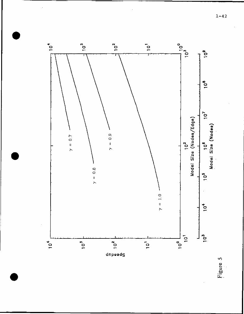
graphs that can be found near the end of the next section. The curves (7 = 1.0) in Figs.

(4-8) illustrate the sequential speedup of this process for six level to two level Trees. These

figures show that the speedup increases as the size of the problem grows. Two scales are

1- 17

provided for model size. One of the scales is for total model size (nodes). The other is for

nodes/edge. Thus, one can relate the equations (nodes/edge) to total model size. Notice that

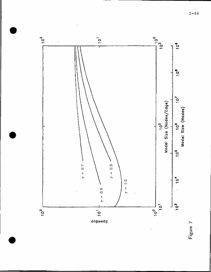
the speedup for a two level Tree, Fig. (8), saturates with increasing model size. This satura-

tion is easily remedied by increasing the number of levels in the Tree. This can be seen by

comparing Fig. (8) to Fig. (7). Also note that increasing the number of levels increases the

speedup, provided that the model is large enough. The curves (7 = 1.0) in Figs. (9-13)

illustrate the memory reduction associated with the External-elimination and Edge-bisection

process for six level to two level Trees. These figures show trends similar to the speedup

trends. Although substantial improvements are shown in these graphs, the desire to extend

the capabilities of the current generation computers to even larger problems leads to further

strategies for improvement.

3.4 Further Strategies for Improvement

While the previous specializations of the HPT have lead to performance gains, the following

methods can lead to further improvements in performance;

• Interpolative Reduction.

• Hybrid Methods.

• Parallelism.

Before parallelism is discussed, the other sequential improvement strategies will be exploited

in the next sections, so that parallelism can further enhance these sequential gains.

/

4 Interpolative Reduction Methodology

The concept of interpolative reduction is to add or provide local information, i.e. stress

concentration, turbulence, etc., in a way that is more economical than grid/mesh refinement.

1-18

Interpolative reduction by levels adds a scaling capability to the HPT, that could be used to

simulate a physical process involving scales [17]. The following methods of interpolative

reduction are discussed.

• Throw-A way Method.

• Substructural Reduction.

• Interpolation.

The throw-away or matrix stripping method is the crudest form of interpolation possible.

In this method, the row and column of the node to be reduced is stripped from the matrix

of externals before passing the matrix to the next level. This process essentially results in

decoupling the equations involving the reduced node from the rest of the system. Since this

is a zero interpolation process, i.e. no information is transferred to any of the surrounding

nodes, this is the cheapest form of interpolative reduction. The substructural reduction

method consists of treating the node to be reduced as an internal node during the substruc-

tural decomposition process, in order to affect interpolative reduction. The following two

constraint methods are used to enforce a nonzero interpolation reduction.

• Energy Method

• Least Squares

After considering the constraint methods of the interpolative reduction process, some con-

sideration must be given as to how this process can be most effectively incorporated within

the HPT process. The interpolative reduction process can be employed at two stages in the

Tree process.

• After Assembly.

• Before Assembly.

1-19

Note that the HPT method bears no similarities to multigrid iterative schemes, where the

results of a coarse grid/mesh are interpolated as an initial guess (preconditioner) to a finer

grid for the purpose of accelerating convergence.

The next subsections discuss the constraint processes and their implementation before

and after assembly.

4.1 Energy Method for Symmetric, Positive Definite Systems

The energy method results in an efficient interpolation, where the energies in both the

original system and the interpolated system have the same average energy. The interpolation

process for symmetric, positive definite systems begins by considering the stiffness equation

resulting from the discretization process.

[K] {Y} = {F} (79)

Then this can be formed into a force residual equation as,

M = [K] {Y} - {F} (80)

From work concepts (F • d r ) , multiply by (7}r.

(Y}T {r} = {Y}T [K] {Y} - {Y}T {F} OT

Thus define an energy residual.

{>•}, = \ {Y}T[K} {Y} -{Y}T{F} (82).

Given the interpolation constraint/curve fit,

{Y} = [7] {7}, (83)

its application to the energy residual yields

{r}e = 1 {Y}T [T]T [K] [7*] {7} - {Y}T [T]T

1- 20

Minimizing the energy residual gives

r}. = mr [K] [T] {Y} - [7T {F} = 0 (85)ay,

Now then the energy interpolation transform is defined.

[K] {Y} = {F} (86)

[£] = [T]r [K] [T] (8?)

{F} = [7]r {F} (88)

However, [K] can be nonsymmetric, nonpositive definite, i.e. for general fluid simula-

tions. This method of minimizing the energy residual to define the interpolative reduction

is not applicable in this situation. Thus, a least squares minimization technique is employed

to prescribe the interpolative reduction process.

4.2 LS Method for Nonsymmetric/Nonpositive Definite Systems

The least squares method results in an interpolation, where the least squares residual is

minimized between the original system and the interpolated system [18-20]. The interpola-

tion process for unsymmetric nonpositive definite systems begins by considering the stiffness

equation resulting from the discretization process. The top level stiffness matrix created by

the FD/FV/FEM/SPE discretization process, (79), can be cast in a residual form, namely

(80). Applying the interpolative reduction (constraint/curve fit) given by (83), the stiffness

matrix formulation and the residual equation yields,

[K] [T] {Y} = {F} (89>

M = [K] [T] {Y} - {F} (9°)

Now apply the least squares method to the above equations by squaring the residual

(r}T W = ([K] (T] {Y} - {F})T ([K] [T] {Y} - {F})

1- 21

and minimizing wrt. to {Y},

4- {r}T {/•} = 0 (92)dY:

yields,

[K]T [T]T ((K] [T] {Y} - {F}) = 0 (93)

Now writing the interpolatively reduced system of equations as,

[*] {Y} = {F} (94)

Comparing equations defines the interpolated stiffness matrix [K] and the interpolated force

vector {F} as

[K] = [T]T (K]r [K] [T] (95>

{F} = [T]T (K]T {F} (96>

Notice that the interpolated stiffness matrix is symmetric and positive definite.

4.3 Interpolation After Substructural Decomposition

Interpolative reduction after substructural decomposition (IRA) process reduces/interpolates

the resultant condensed stiffness matrix, which is composed of the external nodes of the

internal/external segregation process. Then the reduced matrix of externals is transferred

to next level in a downward progression. This reduction process relieves the congestion

occurring at the lower levels. Then starting at the top of the Tree, the next expression

defines the number of nodes at the top of an Ith level Tree.

N, = 1 + (N - l)/(2/-1) (97)

For interpolate reduction after substructural decomposition the number of nodes at the

current level are reduced from the number of nodes at the previous level by the relation.

Nt = 1 + 2(7M NM - 1); i e [1, 7 - 1] (98)

1- 22

where 7,. is the nodes/edge reduction ratio. With the population count defined (97, 98), the

relations given in the appendix (A1-A29) for effort memory and communications are

employed to describe the results of the interpolative reduction after substructural decompo-

sition (IRA) process.

Of course the interpolation could be applied elsewhere in the HPT. Another possibility

would be to consider an interpolative reduction applied before the substructural decomposi-

tion (IRB) process, i.e. directly after assembly. This would allow one more reduction in the

Tree to take place; and, the effort and memory associated with substructural decomposition

phase would be reduced. It was found that the interpolation costs of this method over-

whelmed the aforementioned benefits. Thus, the IRB method will not be discussed further.

The next subsection presents the results of the interpolative reduction after substructural

decomposition (IRA) process.

4.4 Results of Interpolative Reduction

The results of interpolative reduction after substructural decomposition (IRA) process are

displayed graphically in Figs. (4-13) for Edge Bisected, Externals Eliminated, Trees. The

effort associated with various level Trees (6th level to 2nd level) is shown in Figs. (4-8) and

memory in Figs. (9-13). These figures show increases in performance associated with the

following trends:

• increasing the number of levels in the Tree.

• increasing model size.

• increasing interpolative reduction (decreasing 7).

1- 23

The curves in the graphs correspond to equipresent reduction ratios. An equipresent reduc-

tion ratio refers to applying the same reduction ratio to all levels of the Tree. The ratios

used are:

• 7 = 1.0 (no reduction),

• 7 = 0.9 (0.729 global reduction ratio per level),

• 7 = 0.8 (0.512 global reduction ratio per level),

• 7 = 0.7 (0.343 global reduction ratio per level).

The effect of symmetrization can be seen in the jump from the 7 = 1.0 (no reduction) curve

to the 7 = 0.9 curve in each of the figures. Symmetrization is the primary cause of this

jump and the reduction is a minor effect. The jumps between the other curves, excluding

7 = 1.0, show the interpolative reduction effects. As the number of levels increases the

curves begin at larger model sizes. This reflects that the higher level Trees require larger

models. The figures show that the two level Tree is the only tree that cannot pay for the

cost of interpolative reduction, see Figs. (8 and 3).

The range of model sizes covers current and future sized models, where a 100x100x100

3-D model (1 million) equations is considered the practical upper limit of current computers.

The range of the next generation of models is considered to be a decade increase in resolu-

tion in each dimension, or a 100x100x100 3D model (1 million) equations as a lower bound

and a 1000x1000x1000 3-D model (1 Billion) equations as the upper limit of the next genera-

tion of models. In this context the 3-D HPT is showing substantial improvements for current

and next generation models with and without interpolative reduction. These figures fairly

well summarize the sequential 3-D HPT process as presented.

5 Hybrid Methods

Before considering the performance gains available from parallel processing, several

significant remaining aspects of improving sequential processing will be discussed. These

are grouped and classified under the title of hybrid methods.

• Iterative/Direct solve at Root.

• Symmetric/Unsymmetric Formulations.

The first of these hybrid methods considered is that of combining iterative solvers with the

HPT. For certain simulations global iterative solvers can be more effective than global

direct solvers. But again, this is highly problem dependent. In these situations the root

burden can be reduced by an efficient iterative solver of the following types:

• steepest descent.

• preconditioned conjugate gradient.

The effort improvement depends on the rate of convergence which, in turn, is dependent on

the particular implementation of the iterative solver, the initial guess used to start the solver,

the particular simulation, and ratio of the root burden to the overall computational burden.

Previously it has been demonstrated that even through the use of multilevel edge bisection,

which has been employed to reduce the root burden, the root is the single largest HPT

burden. The memory (number of memory locations) for the iterative solver is now

equivalent to the number of equations (Ne), assuming that the iterative solver requires

auxiliary storage much less than 0(Ne). This represents two orders of magnitude of

improvement in the root memory requirements. Thus, the iterative/direct hybrid HPT is an

effective strategy, when applicable. The applicability can be determined on the fly, by

monitoring the rate of convergence, comparing the accumulating solve effort to estimated

1- 25

direct solve effort. If the rate of convergence deteriorates or the solve effort exceeds that

of the direct solver, the program can then switch to the direct solver. The beforehand

checks that could be employed are the matrix condition number of the system. Certain

formulations of certain simulations are known, apriori, to have poor condition numbers for

convergence. Matrix density is another parameter that can be tested. Iterative techniques

are not generally used to invert full matricesj because there is no savings in storage, the

effort savings due to sparsity has disappeared, and they do not generally have good

convergence properties.

The second hybrid method considered is that of the symmetric/unsymmetric HPT.

There are two considerations. First, the least squares interpolation method has been shown

to symmetrize the system matrix resulting from discretization processes. If this

symmetrization is taken advantage of at the top of the tree then memory reduction and

speedup gains occur at each and every successive level in the tree, by halving the

computational effort and memory requirements. The second consideration of the symmetric/

unsymmetric hybrid HPT is the consideration of regions that may be either a symmetric or

unsymmetric formulation within the same simulation, e.g. fluid-structure interaction

simulations. Thus, the HPT has capability to regularize a model, in terms of merging a

symmetric/unsymmetric problem into a symmetric one.

6 Parallelization of HPT

In parallel computing environments, the tree structure can be used to establish the flow of

control, communications and problem assembly. Overall, several types of parallel archi-

tecture can be defined for the foregoing HPT formulation. These include:

1-26

1. Fully parallelized, wherein each partition of the tree is provided its own processor

with either shared or local memory.

2. Partially parallelized, wherein P singly assigned processors are leapfrogged from

substructure to substructure level by level, see Fig. (14), or

3. Partially parallelized, wherein a total of P processors are organized into G groups

which are separately leapfrogged to various partitions, level by level, such that

several processors may be assigned to a given partition, Fig. (15).

Note for case 3) involving multiple assignment, since such architectures tend to reach

saturation when too many processors are locally involved, the choice of P and G is machine

dependent. Here of course the main goal is to maximize the superlinearity. A further aspect

of cases ii) and iii) follows from the fact that as the forward elimination process moves down

the tree, the number of processors may become greater than that of the branches. For such

situations, the multiple assignment factor P/G may be raised to improve utility; if saturation

is not reached.

Based on the prior comments on parallelism, the expression defining Fe needs to be

altered. In particular, modifications must be introduced to account for such features as full/

partial parallelism, single/multiple assignment and, single/multi processor efficiency. This

process leads to the following formulations:

i) 2-D fully parallel

Pf{Fe} » 6.12 P\k2 + 1) N* + [£28.1 P3(£.+1 + 1) (tf.)3 + 9 P

3(^)4 (99)L'=2

ii) 2-D partially parallel-single/multi assignment

(100)

1-27

E P \f_i '

{Fe}pl » 6.12 p>(k2 H- 1) (tf)3/(E P) (103)

iii) 3-D fully parallel,

P,{Fe} ~ 27 p3(fc2 + 1) N6 + [£ 108 P3(*M + 1) (A^.)61 + 16 P

3(^)7 (104)L<=2 J

iv) 3-D partially parallel-single/multi assignment

= E (^V (105)1=1

- 27 P\k2 + 1) (JV)6/(E P) (108)

such that E denotes machinery efficiency. Noting case ii), the speedup potential afforded

by employing the HPT framework to parallelize calculations can be very significant. For

example considering the two level tree, then for 2-D simulations,

Pp{S} ~ 0(NW) E P (109)

and for 3-D simulations,

Pp{S] ~ 0(tf4/5) E P (HO)

Depending on problem size, even better optimalities are afforded by introducing multiple

branch levels. The partially parallelized HPT yields the following effort requirement namely

Pp{Fe(net)} = ~{Fe(root) + Nc Fe(itnit cell}} (HI)

1- 28

Equation (111) can be interpreted in two ways. In particular, the unit cells can be handled

via either single or multiple assignment leapfrogging. For the single case, only one

processor is scheduled to handle a given partition's operational needs. These requirements

change depending on whether the forward elimination or back substitution phases of compu-

tation are involved. Note that the forward phase involves a downward flow of control in the

tree. In contrast, back substitution requires an upward flow of control. For the multiple

assignment architecture, the various operational steps are shared among the various

processors scheduled for the given substructure. If multi-assignment processor saturation

is taken into account, then (111) reduces to the form

Pps{Fe(nef)} = -J—{Fe(root) + Nc Fe(unit cell)} (112)E Ps

where P5 denotes the allowable upper bound on the number of processors that can be

dedicated to a given programming task. In the case where Ps < P is satisfied at all the

various branch levels, then (111) reverts to (112).

7 Discussion and Conclusions

This paper has presented the results of an analytic investigation into the characteristics of

a unified parallel processing strategy for implicit, three dimensional formulations. For 2-D

and 3-D FD/FV/FEM/SE models, the HPT offers very attractive asymptotic computational

speedups, memory reductions and minimized communications. In a coarse-grained parallel

computing environment, where processor leapfrogging is employed to handle the tree, the

effort reduction is proportional to E P, namely for 2-D models

P{5) ~ 0(N2n) E P

and for 3-D models

1-29

P{S} - O{(Problem Size)4'5} E P (114)

Note since the Tree provides for individual updating of each of the top level branches, the

model stiffness regeneration effort is reduced by the same factor (E P). Overall, the HPT

forms a naturally parallelizable communications link. Since it minimizes memory and effort,

hardware demands are also reduced. This is not the case with recent attempts at parallelizing

direct global solvers, which leave the memory and effort requirements unchanged. In addi-

tion to finding large reductions in memory, communications, and computational effort

associated with a parallel computing environment, substantial reductions have been generated

in the sequential mode of application. Such improvements grow with increasing problem

size. In the case of models with relatively cubic morphologies, as problem size becomes

very large, the following asymptotic, many orders of magnitude, effort and memory reduc-

tions occur for sequential computer environments, namely for 2-D simulations,

S ~ C){(Problem Size)2'3} (115>

Mr ~ <9{(Problem Size)1-'3} (116)

and for 3-D simulations,

S - <9{(Problem Size)4'5} (117)

Mr - 0{(Problem Size)2''5} (118)

Similar trends apply for the communications requirements. Optimality considerations were

given to these performance factors, showing i.) how the 3-D Tree can be tuned for peak

performance, and ii.) some results of this tuning process.

In addition to a theoretical development of the general 3-D HPT methodology, several

techniques, for expanding the problem size that the current generation of computers are

capable of solving, have been presented and discussed. Among these techniques that have

!- 30

been discussed, are several interpolative reduction methods. Some of these techniques have

2-D applications as well. It was found that by combining several of these techniques that

a relatively small interpolative reduction resulted in substantial performance gains. Possibly

the most significant finding was that previously prohibitively computationally expensive pro-

cedures can be employed at the top level of a multi-level tree without significantly affecting

memory, communications and computational effort. For example, least squares formulations

are particularly effective when the system of governing equations are cast in a first order

form. This removes two major difficulties. First the inter-element continuity requirements

are lowered. And second, the problems associated with terms of different order, e.g. the

pressure and velocity terms in an incompressible flow simulation or in the case of modeling

of incompressible materials, disappears. These gains are obtained at the cost of increasing

the size of the system of equations that must be solved. Due to the already overburdened

and limited capacity of current generation computers, the potential of least squares and other

computationally expensive formulations have not been exploited on a large scale. However,

when employed at the top level of a hybrid multi-level Tree these previously prohibitively

computationally expensive procedures become very cost effective.

It should be pointed out that, it is expected that in practice one will find the speedups

and memory reductions to be larger than those projected in this paper for two main reasons:

• The assumptions that the analytic expressions have been based on, are conserva-

tive; and in practice,

• the system matrix of each partition on each level can be optimized before substruc-

tural condensation or solution.

1- 31

,^^ - Numerical studies and applications of the HPT have verified the assertion that the analytic

expressions are conservative for both sequential and parallel computations for the 2-D Tree.

It is hoped that the results of this work will be useful in the design and implementation of

the next generation of computing hardware.

References - Part One

[1] AJ. Baker, Finite Element Computational Fluid Mechanics, McGraw-Hill, N.Y., 1983.

[2] Thomas H. Pulliam, Implicit Methods in CFD, Eds. K.W. Morton and M.J. Baines,

Numerical Methods for Fluid Dynamics and Aerodynamics III, Clarendon Press, 1988.

[3] K: Gallivan, A. Sameh and Z. Zlative, A Parallel Hybrid Sparse Linear Systems

Solver, Computing Systems in Engineering, Vol. 1, Nos. 2-4, pp. 183, 195, 1990.

[4] C. Cuvelier, A. Segal and A.A. Von Steenhoven, F.E.M. and N-S Equations, D.

Reidel, Boston, 1986.

[5] J. Padovan, Nonlinear Hierarchical Substructural Parallelism and Computer Archi-

tecture, Computational Mechanics CSM Workshop presented at NASA-Langley, June

1985.

[6] J. Padovan, D. Gute, and K. Johnson, Hierarchical Poly Tree Computer Architectures

Defined by Computational Multidisciplinary Mechanics, Computers and Structures,

Vol. 32, No. 5, pp. 1133-1163, 1989.

[7] D. Gute, Hierarchical Poly Tree Computer Architectures for the Solution of Finite

Element Formulations, Ph.D. Dissertation, University of Akron, January 1990.

[8] J. Padovan and A. Kwang, Hierarchically Parallelized Constrained Nonlinear Solvers

with Automated Substructuring, Vol. 41, No. 1, pp. 7-33, 1991.

1- 32

[9] J. Parris, Hierarchical Poly Tree Methodology and Partitioned Implicit Fluid

Simulations, Ph.D. Dissertation, University of Akron, May 1992.

[10] C.M. Albone, An Approach to Geometric and Flow Complexity Using Feature-

Associated Mesh Embedding (FAME): Strategy and First Results, Eds. K.W. Morton

and M.J. Baines, Numerical Methods for Fluid Dynamics and Aerodynamics III,

Clarendon Press, pp. 215-235, 1988.

[11] X. Cai and O. Widlund, Domain Decomposition Algorithms for Indefine Elliptic

Problems, Siam J. Sci. Stat. Comput., Vol. 13, pp. 243-258, 1992.

[12] A. George and J. Liu, Computer Solution of Large Sparse Positive Definite Systems,

Prentice-Hall, Englewood Cliffs, N.J., 1981.

[13] E. Cuthill and J. McKee, Reducing the Bandwidth of Sparse Symmetric Matrices, Proc.

ACM National Conference, pp. 157-172, 1969.

[14] N.E. Gibbs, W.G. Poole, and P.K. Stockmeyer, An Algorithm for Reducing the Band-

width and Profile of a Sparse Matrix, SIAM Journal of Numerical Analysis, Vol. 13,

pp. 236-250, 1976.

[15] K.J. Bathe, Finite Element Procedures in Engineering Analysis, Prentice-Hall, Engle-

wood Cliffs, N.J., 1982.

[16] M.M. Denn, Optimization by Variational Methods, McGraw-Hill, N.Y., 1969.

[17] A.J. Reynolds, Turbulent Flows in Engineering, Wiley, N.Y., 1974.

[18] P.P. Lynn and S.K. Arya, Use of the Least Squares Criterion in the Finite Element

Formulation, International Journal for Numerical Methods in Engineering, Vol. 6, pp.

75-88, 1973.

l- 33

[19] C.A.J. Fletcher, A Primative Variable Finite Element Formulation for Inviscid,

Compressible Flow; Journal of Computational Physics, Vol. 33, pp. 301-312, 1979.

[20] B.N. Jiang and G.F. Carey, Adaptive Refinement for Least-Squares Finite Elements

with Element-by-Element Conjugate Gradient Solution, International Journal for

Numerical Methods in Engineering, Vol. 24, pp. 569-580, 1987.

1-34

Appendix

HPT Effort Memory and Communications Burden associated with external-elimination and

edge-bisection.

1) Effort

Fe = £ (Fe\ (A1)1=1

(Fe}, = 8 [(7V3S),. (F«M), + (N4S\ (Fe4s),

>, + <*«>, (**«>J (A2)

(Fe35), » p3[25/v7 - 1057V/ + 1847V/ -

1Q6N? - 4QN? + 9AT; - 1] (A3)

(Fe4S); » ip3[36^77 - 204N/ + 469N/ - 5882V/ +

449N,3 - 214N/ + 6QN, - 8] (A4)

(Fe5s)j » ip3[49^/ - 357A?/6 + 1,0722V/ - 1,756/V/ +

1,744/V/ - 1,072/V7 + 384/V7 - 64] (A5)

(Fe6s)/ « 4P3[4/V7 - 36/V/ + 137/V/ - 290/V,4 +

376/V/ - 304/V/ + 144/V7 - 32] - (A6)

f - 25,705/V/ + 125,225/V/ -

329,654/V3 + 494,316/vf - 400,257/V. + 136,725] (A7)

(Fe4S). -,- p3[3,737/V/ - 41,998/V/ + 200,645/V/ -

518,746/V,3 + 761,8377V;2 - 599,776/V. + 197,181] (A8)

). ~ -lp3[5,865/V,6 - 56,0297V/ + 231,2187V/ -48

525,2547V/ + 691,2737V/ - 499,4617V,. + 155,28] (A9)

1- 35

), - -Ip3[8,977/Vf - 56,590V? + 244,730/7' -

560,564/V,3 + 718,1977V:2 - 505,104/7, + 156,024] (A 10)

i e [2, 7 - 1]

j » -Lp3[2llNf - 3,1577V* + 19,148/7* -

62,0547V3 + 113,481/7' - 111,189/7. + 45,666] (All)

2) Memory

Me =

4

(Me\ = 8

),] (A13)

(Me3S), « p2[52V/ - UN? + 8Nf - 6N? + 3N, - 1] (A14)

(Me,s), ** P2(6N? - ISNf + \3N? - 9N? + 5N, - 2] (A15)

75 - 207V/ + 21//7

3 - 14JV/ + 8^V7 - 4] (A16)

^3 - 23N? + 12^ - 8] (A17)

(Me3S). » p2[58A^/ - 45QN? + 1,341/7' - 1,816/7. + 943] (A18)

(Me4S). » Ip2[162N/ - l,205/73 + 3,4517V/ - 4,491/7,. + 2,235] (A19)

(Mess\ » Ip2[217/V/ - 1,400/V3 + 3,586/V/ - 4,288/7. + 2,037] (A20)

(Me6s),. » ip2[285/V' - 1,403/V3 + 3,595/7/ - 4,301/7. + 2,040] (A21)

[2,1- 1]

1-36

(Me\ « -p2{21Nf - 266N? + 9802V/ - 1,6022V. + 981] (A22)

3) Communications

Ce = £ (Cc), (A23)i=2

(00, = 8

+ (Wi,)( (Ce,,), - (/V6S),. (Ce6S),.] (A24)

(C«M)f - P2[37V,2 - 3/V,. + I]2 (A25)

(Cc45)f » p2[4/V/ - 5/V, * 2]2 (A26)

(Cess), » p2[5/V/ - 8/V. + 4]2 (A27)

(Ceu)t ~ p2[6/V2 - 12/V,. + 8]2 (A28)

i e [2,7]

whereTV. = 1 + (N - l)/(2'"-1); z e [2, 7] (A29)

1-37

Figure Legend - Part One

Fig. 1 Globally minimized model, stiffness matrix population.

Fig. 2 Bandwidth expansion by sub structuring row column placement.

Fig. 3 Multilevel edge-bisection of 3-D cube.

Fig. 4 Speedup for a 6 level edge-bisected tree.

Fig. 5 Speedup for a 5 level edge-bisected tree.

Fig. 6 Speedup for a 4 level edge-bisected tree.

Fig. 7 Speedup for a 3 level edge-bisected tree.

Fig. 8 Speedup for a 2 level edge-bisected tree.

Fig. 9 Memory reduction for a 6 level edge-bisected tree.

Fig. 10 Memory reduction for a 5 level edge-bisected tree.

Fig. 11 Memory reduction for a 4 level edge-bisected tree.

Fig. 12 Memory reduction for a 3 level edge-bisected tree.

Fig. 13 Memory reduction for a 2 level edge-bisected tree.

Fig. 14 Sequential processor assignment, and partially parallel single processor assignment.

Fig. 15 Partially parallel, multiple processor assignment.

1-38

2-D

i+N

\ 3-D

i-N

Figure 1

1-39

QCd

C*DHU

HenPQDC/3

QCdS3

cuO

CM

2

1-40

00

<D

1-41

ino

OO

IOO

ooO

03.C)

o>

nu

oN

CO

0>-oo

mo

NCO

TJo2.

inO

nO

nO

CMo

oO

dnpaadg

2

1-42

KJ

oOO

CO

o

nO

coO

1x1

0)o

T3N -2o z

N

O•DO

Oz

V)

inO

inO

CMO

OO

dnpsads10O -

E

1-43

CM

OOo

10o

0O

0O

oo>

01<D

XIO

en

*o•oo

OJo

TJOz

N

en

"5-oo

inO

10O

KJO

NO

Oo

dnpaadg vO

1-44

CMo

oo

aO

ooO

o

no>•oo

0>N

uT3O

no-oo

V}

"5TJO

inO

nO

O

dnpaads

oo

P

£

1-45

0>o

COo

CM

Oa>

TJ

nu

TOo

oNtna•ao

COO

Oz

o

</>

"oo

nO

CM

dnpaads

oo

W)

1-46

ooCM

Om

oo o

m 09T O

CMO

Oo>TJLU\woTJo

o-oo

r-.o

ao•ao

o «en~oTJO

nO

OO<N

Om

oo

om

1-47

oto

oin

oCM OK,

o

qi—I

II

-i o

10O

Q>o>

ofjo>

T3N £O 2^

0>N

C/J

^o

ra

ozN^

O

tn"oo

inO

O(O

oro

oCM

uojpnpay

3

£.

1-48

oCM in

Oo>•aui\m

N £o z

N

en

-oo

a •O

(9O

TOO

o »,_ N

en

"oo

Mlo

oeg

uo^onpay

CM 10o

0)Qi

UJ

mTJ

M O

°S

N

C/J

~oTJO

(0O

01O

-oozv^

to

2.8C/J

"oT3O

IOO

nO

CM

tuO

1-50

CM

oo>-oLU\

COV

N\n

-oo

o -1 o

o>o

(0o

nv

TJo

<D

° 5

-oo

<N

1-51

Cd>Cd

L

Cc

OO

O§00

OuCO

o

1-52

J

bJO

Hierarchically Partitioned Solution Strategy ForCFD Applications: Part II - Numerical Applications

Joe PadovanA

Departments of Mechanical and Polymer EngineeringThe University of AkronAkron, Ohio 44325-3903

Abstract

Part I of this series presented an analytical investigation of the use of HPT fluid

simulations along with extensions to parallel computer environments. This was achieved in

a closed form sense for simplified geometries. In Part II, the work will be numerically

extended to handle more complex geometric morphologies. Specifically, the structure of the

tree is optimized numerically contingent on problem dependent resource requirements. This

is followed up with the results of several comprehensive implicit CFD simulation studies

which demonstrate the effectiveness of the HPT concept.

1 Introduction

This part of the sequence presents the results of research in the area of parallel computer

processing with Computational Fluid Dynamic (CFD) applications. The concept of Hierar-

chical Poly Trees (HPT) [1] is applied to prototypical CFD applications resulting in lower

bound approximations to computational effort and memory requirements. Briefly stated,

HPT implements multilevel substructural decomposition to achieve reductions in memory,

computational effort, and communication requirements. For 2-D sequential problem formu-

lations, the asymptotic upper bound trends show a square root of problem size reduction in

effort and concomitantly, a fourth root reduction in memory requirements. In this context,

as the model size increases, the HPT methodology shows increasing computer effectiveness

in terms of both memory and computational effort. The HPT methodology extends this

sequential performance improvement to the parallel processing environment in such a natural

way that system overhead is minimized. Additionally, the HPT can be employed at the

modeling stage, i.e. a preprocessor capable of taking advantage of, and indeed simplifying,

modeling tasks such as geometric cell cloning, a feature associated mesh enrichment (FAME)

[2] etc. We will show the optimal HPT to be dependent on the geometric features of the

model. Once the HPT has been optimized (OHPT), it is not necessary to perform this task

again and can be saved for future use. Hence, libraries of Optimized Hierarchical Polytree

substructures (LOHPTS) can be developed. The HPT methodology is general enough to be

applied to existing FD/FV/FEM CFD codes without an extensive rewriting of code and can

be implemented on existing parallel computer architectures. OHPTs have additional benefits

of being able to reconfigure parallel computing resources in a problem dependent optimal

arrangement, something that other parallel computing strategies lack.

The sections that follow will provide: 1) a brief discussion of the CFD equations

involved; 2) a numerical optimization scheme to define the tree structure for general problem

geometric morphologies and; 3) its effects on parallelization. Included are the results of

several large scale benchmark CFD applications. These illustrate the significant speedup

potential and memory/communications reduction for typically sized incompressible flow

models.

2 FE/FD Models - Implicit CFD Formulations

For discussion purposes consider the spatially discretized CFD system of equations of the

general first order, nonlinear form;

[M] + [*(Y)] {v} = {F}, (1)at

where

{v} = {v,, v2, v3, p, TY, (2)

[M] is the mass matrix, and [K(v)] the nonlinear effective stiffness matrix. For a heat

conducting incompressible fluid flow and either a FD or FE formulation [3], the general

form of the stiffness matrix is given as,

(K(v)] = [Kc(v)] + [Kd] (3)

The stiffness matrix is composed of [Kd], a symmetric diffusion matrix, and [Kc(v)], an

unsymmetric convection matrix. In the primitive variable formulation, the symmetric

diffusion matrix also, contains the contributions from the pressure and the continuity

equation. For discussion purposes, consider the two dimensional element for incompressible

viscous fluid flow as used in the FE computer program ADINA-F [4,5]. This 9 node

element is of second order in velocity and temperature, and linear in pressure to insure

2 - 3

stability via the Babuska-Brezzi condition [6,7]. Then the element mass and stiffness

matrices are formed as,

[M] =

[K] =

[ 0 ]

[*„] [ 0 ] [K13] [ 0 ]

[0] [K22] [K23] [0]

[K13f [K2JT [ 0 ] [ 0 ]

[K4I] [K,2] [ 0 ] [K44]

(4)

(5)

A development of the submatrices [Mn] and [Kti] can be found in Bathe [4,5]. Noting (5),

the stiffness matrix is essentially full. This fullness of the stiffness matrix translates to large

bandwidth and problem size. The velocity coupling terms [K12] and [K2i] are equal to zero

as a result of using the traditional Galerkin approach. In other formulations, these terms are

not zero [8]. Also other coupling blocks, [K14] and Ku], need not be zero [9]. In light of

this, the most general formulation has a full element stiffness matrix. When the element

matrices are assembled into the global stiffness matrix, a symmetric profile is created whose

entries are not symmetric, i.e. K{j j± Kj{.

2.1 Steady State Formulation

The steady state formulation, obtained by dropping the partial time derivatives from (10) is

then,

[ff(v)] {v} = {F} (®

This nonlinear system is not directly solvable. Hence, an iterative procedure is the only

method of solution. Typically successive substitution also known as fixed point iteration,

2 . 4

Picard iteration, or successive approximation is employed. Newton's method is generally

relied on for problems with strong nonlinearities. This is a result of its asymptotic quadratic

convergence rate. The application of Newton's method to (6) yields

•MM = M,where

[/] =

In either case, matrix inversion is required. The solution to a steady state problem can also

be given as the time asymptotic limit to an equivalent transient simulation. This approach

is often preferred since it is history dependent and doesn't jump to different history depen-

dent loading states.

2.2 Transient Formulation

After spatial semi-discretization (FD, FV, or FEM), all that is required for solution, is the

resolution of the implicit temporal operator. This is accomplished in a variety of ways, e.g.

the a method [10], predictor-corrector method [9], and other ODE solvers. The advantage

of using high order ODE solvers, i.e. Gear's method, on the semi-discrete form, are negated

by

• errors due to spatial discretization and

• nonlinear terms.

After the resolution of the temporal operator, the transient problem takes the form,

[KD(v)] {v} = {FD}, (9)

where [KD(v)] is the dynamic stiffness matrix, and {FD} is the dynamic load vector. Thus

a nonlinear set of equations, that resemble the steady-state formulation, must be solved at

2 1- 5

each time step. For transient problems, each time step is chosen close enough to the

previous one to use Newton's method. In practice, it has been found that it is desirable to

control the error tolerance, such that a balance of one Newton iteration per time step is

achieved. Let 7 equal the HPT work reduction, then the resultant work effort for implicit

transient solvers is 7 times the work effort (Eff) prior to the application of the HPT

methodology, i.e.

E ffHpT = jEf f (steady-state) (10)

EffHPT = y Eff (transient) (11)

Thus the governing field equations have been reduced to solving repeatedly a large, sparse,

unsymmetric system of implicit linear equations. Although we have illustrated the case of

incompressible fluid flow, this also is true of compressible flow and more general continuum

problems. With this in mind, we begin applications of the HPT methodology to four real

world computational fluid dynamics models to benchmark the analytic results presented in

Part I.

3 Application of the HPT Scheme to Real World CFD Applications

In Part I, we have shown analytically, via operations counts and symbolic algebra for square

2-D and cubic 3-D morphologies the HPT methodology capable of i) reducing the computa-

tional effort required for direct inversion of fluid simulations, ii) reducing the memory

requirements, and iii) reducing the communications burdens. The analytics of the HPT

methodology exhibit for a given model optional substructuring in terms of the number of

levels and the number of substructures per level. In general arbitrary substructuring

produces suboptimal results. Additionally the potential of the method to exploit coarse and

fine-grained parallel computer architectures was briefly discussed.

2l- 6

It was necessary to base the analytic work on a regular (square and cubic) geometry to

obtain a node numbering pattern to formulate analytic expressions of computational effort,

memory and communications burdens. Real world models rarely have square or cubic

morphologies. This led to the work of Padovan and Kwang who have automated the sub-

structuring process [11]. Kwang's AUTOSUB program [12] numerically tallys the computa-

tional effort, memory and communications burden for arbitrarily shaped, multiply connected

2-D regions. The following sections of this paper discuss the application of the HPT

methodology, outline the automated substructuring process and present four benchmark CFD

applications to reinforce the analytic results presented in Part I.

The HPT process begins by hierarchically partitioning the model into multilevel

substructures. Such a process is illustrated in Fig. (1). Typical of FD models, the double

airfoil simulation described in Fig. (1) can be mapped into its topological equivalent, see

Fig. (2). The overall process extends to more elaborate multibody grids, with more complex

unit cells. Consider the modeling of the fluid flow around a stator blade cascade in the

turbine section of a jet engine. Figure (3) illustrates a typical blade set, i.e., the first stator

vane. Noting the periodicity, one can see that there is a recurring unit cell model. As can

be seen from Fig. (3) the connectivity between cells consists of a row of repeated boundary

nodes. This node row determines the root of the HPT. The second level branches are the

unit cells. This is described in Fig. (4). Usually the cell is defined by many nodes. As a

result, additional levels may be required to reduce the cell level computational effort,

memory utilization and communications costs. For demonstration purposes, assume that the

cell is a 2-D square. To balance the tree, we must decompose the cell into partitions which

yield the minimum external/internal ratios. This is achieved for square zone shapes. Figure

2 ;- 7

(5) illustrates a typical multilevel partitioning of the cell to establish the zone sizes and

number of levels, the Gaussian elimination process is relied on to determine the operations

count. Since the forward matrix reduction phase requires the major effort, it is used to

structure the tree architecture. Recall that the cell level requirements have been addressed

in Part I of this paper.

Now the root level effort, memory and communications requirements can be deter-

mined. Recall that the root here consists of a cell interconnecting node row, i.e. Fig. (3.6).

As a result of the forward elimination process performed at the branch levels, the condensed

'stiffness' linking the interconnecting nodes of the unit cells are fully populated. In this

context, the root level assembly yields a matrix with a regular skyline height of 0(3pNr) such

that Nr denotes the number of upstream-downstream interconnect nodes at a given unit cell

interface. Given Nc uni t cells, the net size of the assembled root 'stiffness' is 2pNr(Nc + 1).

Hence the root level effort is

Fe(root) = 18 P3(NC + 1) (A^)3 (12)

The associated memory and communications requirements are defined by

Me(root) = 12 P2(Nc + 1) (Nr)

2 (13)

Ce(root) = 16 p1 Nc(Nr)2 (14)

Note, because of the regular form of the root of the blade cascade problem, reduction into

its own HPT will not decrease its effort. Rather, to yield an improved tree, the only

recourse is to agglomerate unit cells into larger repeated substructure. Such enlarged cells

would then be treated in the same manner as before.

2 - 8

Employing (12-14) and the following expressions from Part I (15), (17), (21) we yield

the following expression for the sequential formulation of the HPT associated with the

cascade problem, namely

Fe(net) = Fe(root) + NcFe(unit cell) (15)

Me(nef) = Me(root) + NcMe(unit cell) (16)

Ce(rcer) = Ce(root) + NcCe(unit cell) (17)

Optimization of the overall tree would follow as before. In the case that the root is treated

as a single partition, then optimization would be performed only on the unit cell. In a later

section, some trend studies will be overviewed to illustrate the benefits of the HPT.

3.1 Analytical-Numerical HPT Optimization

For problems composed of purely rectilinear cells, the foregoing development can directly

handle the optimized structuring of the HPT architecture. In the case of more general forms

of connectivity, an alternative approach must be employed. This of course is highly problem

dependent. Generally, in fluids problems solved via the FD scheme, mesh connectivities are

usually highly rectangular in nature. Hence, the associated HPT can be developed in a

manner similar to that employed for the above noted turbine blade row problem. In contrast,

FE meshes generally lead to relatively more complex nodal connectivities. This of course

renders the direct analytical tinkering with the skyline too cumbersome an approach. To

circumvent these difficulties, an alternative numerical procedure will be employed [11].

Overall the method consists of several phases of tree structuring, these include:

• phase 1; choose number of levels and branches per level.

• phase 2; decompose a given level into individual partitions.

• phase 3; bandwidth minimize internal degrees of freedom of each substructure.

• phase 4; compare performance characteristics of various parametrically varied tree

configurations to establish optimal construct.

For the current purposes, a golden section search [13] methodology is employed to

define the proper branch count for each level. In this method, the branching is not selected

arbitrarily. Rather, it is defined through the golden ratio which is obtained from the

appropriate Fibonacci sequence [13]. Alternatively, the Fibonacci search scheme [13] can

also be employed. Here, it must be recognized that we are dealing with an integerized

space. In this context, the search is rounded to the appropriate nearest integer value. To

start the procedure, the overall external-internal degree of freedom ratio is used to define a

rectangular region of like size. The HPT arising from the rectilinear model is then used to

start the search. The central feature of the process is the automatic partitioning scheme.

The main difficulty of partitioning is the need to establish the minimum external to internal

ratio. Since mesh generation is prototypically geared to geometry and physical modeling

needs, it is difficult to generalize the process. To circumvent this situation, an incremental

agglomerational process based on localized node connectivity will be employed. In

particular the procedure consists of several operational steps, namely:

1. Seeding the starting point of agglomeration.

2. Adjoin neighboring nodes in successive waves of attachment.

3. Terminate attachment when present partition size is reached.

4. Bandwidth minimize partition just generated.

5. Subtract agglomerated substructure and determine next seeding point.

6. Repeat reseeding, agglomeration, local bandwidth minimization, and substructural

subtraction until the prescribed number of partitions is reached.

2 -- 10

Figures (3.8 and 3.9) illustrate the dissection process of a tube bundle. Both single and

multiple seedings are illustrated. As noted, such operations are repeated for each branch of

the given level.

The starting/seeding point about which the adjoining process is initiated, is chosen to

be nodes with the least connectivity, i.e. outside corners existing either in the original mesh

or in the reduced mesh resulting from several partition deletions. Since many such points

may exist in both the original and successively reduced mesh, the optimal choice is through

the use of bandwidth minimization, i.e. via Cuthill-McKee [14] or Gibbs-Poole-Stockmeyer

[15]. In particular the lead node of the optimized connectivity is declared the seed point.

As seen in Fig. (6), for symmetric structures, simultaneous seeding and agglomeration is

possible.

Once the starting point is established, the adjoining process can begin. To preserve the

maximum bandwidth compactness for the given partition, the map of directly connected

nodes is used to agglomerate mesh in successive waves of attachment. This process is illus-

trated in Figs. (6 and 7). Several factors control the attachment process: 1) the number of

degrees of freedom per node, ii) the connectivities of nodes neighboring an already attached

zone, iii) the degree of connectivity a node has within a given partition, and iv) the number

of degrees of freedom the partition has been configured to contain. The issue of the degree

of attachment that a given node possesses, has great bearing on controlling the generation

of salients on the boundary (planar, 3-D) of partitions. In complex multiply-connected

geometries, i.e. possessing holes, the agglomeration process can become trapped in salients

or branched configurations. In such situations, weakly attached nodes in such boundary

2 ;.- 11

regions can be reattached to surrounding partitions provided a higher level of connectivity

is generated.

Overall the process of partitioning is performed at each level for all associated

branches. Once a given branch is completed, it is treated as a full structure at the next

higher tree level. In particular, it is partitioned in the same manner in successive applica-

tions of the foregoing decomposition process.

4 Benchmark Applications

To illustrate the speedup potential of the HPT scheme, the results of several benchmark

studies will be considered. These include:

1. harbor model

2. airfoil model-multiple cell

3. turbine blade models-multiple cells

4. tube bundle assembly

The numerical experiments were conducted on a vectorized IBM 3090-200 employing

extended memory architecture to provide for more primary (i.e. paged) memory. The soft-

ware created to automate the hierarchical substructuring of the mesh used a combination of

Cuthill-McKee [14] and Gibbs-Poole-Stockmeyer [15] bandwidth minimization to both seed

agglomeration as well as define optimal partition level node numbering. The direct solver

used to effect the solution was based on the traditional Wilson [10] type LU decomposition

scheme employing skyline storage. The scheme was reformulated to profile style elimina-

tion. This enabled a more efficient use of multiple processor assignment for parallel studies.

The main thrust of the empirical work is to determine the speedup potential afforded

by the HPT. A second interest is to establish the effects of geometry and geometric and

2 :.- 12

node connectivity variations. In this context, several types of mesh and geometry

configuration were considered, in particular,

• branched topologies (harbor model)

• periodically repeating unit cells (turbine model)

• multiply connected domains (tube bundle)

• problems involving complex transitions in mesh connectivity (tube bundle)

Note since various of the problems considered have rectilinear type unit cells, the capability

of the auto-mesh partitioning scheme can be tested against theoretical results. To provide

a fair evaluation of speedup, the HPT results are compared with the global model employing

a combination of Cuthill-McKee [14] and Gibbs-Poole-Stockmeyer [15] type minimization.

Beyond just testing treed versus global formulations, such studies enabled a comparison

between the traditional bandwidth minimization procedures and the current partitioned

approach. As will be seen from the results which follow, each geometric and connectivity

arrangement has its own generic so called optimal HPT, i.e. the OHPT. In particular, each

distinct internal and external boundary configuration and concomitant mesh topology will

have a unique OHPT which minimizes effort, memory and communications. It is possible

that a given model might have several so called local OHPT. The analytical solution of such

nonlinear problem posses a real challenge in optimization. Two examples to follow, illus-

trate the numerical solution to the problem of determining the OHPT.

4.1 Harbor Model: Branched Topology

For the first test, we shall consider the Charleston harbor model of Johnson et al [16].

Figure (8) illustrates the boundary-fitted coordinate system. The associated mesh connec-

tivity is given in Fig. (9). Since branched multiple connected spaces tend to degenerate the

2 ..- 13

bandwidth minimization process, the problem provides a realistic assessment of the speedup

potential. Based on the automatic optimal decomposition, Table (1) illustrates the OHPT for

two and three level configurations. As can be seen, significant speedups are recorded for

the sequential applications of the OHPT, i.e. 2.50 (2 level) and 5.31 (3 level). Employed

in a coarse grained four processor environment, the IBM 3090-400, the respective speedups

are 7.75 and 16.9. Overall, use of the OHPT enables a significant reduction in crunch time.

Concomitantly, the savings in storage obtained was a factor of 2.37 for the three level tree.

Recalling the square topology asymptotic speedup and memory reduction, it follows that for

the sequential case, memory reduction and speedup are proportioned by the relationship

Memory Reduction = O wspeedup i (1°)

As these savings are size dependent, the method generates improved performance with

increasing problem size.

4.2 Airfoil Model: Multiply Connected Unit Cell

To simplify the modeling scheme, we will employ the traditional slender body mapping

technique to determine the airfoil model [17]. Figure (10) illustrates the foil simulation and

the topology of its node interconnection. Based on the noted configuration, Fig. (11) gives

the speedup potential for various two level HPT structures. As can be seen, there are

several local minima leading to relative OHPT. Overall, the global OHPT yielded a

sequential speedup of 4.62 for the case of a four airfoil stack. For the three level tree, a

speedup of 11.8 was recorded. The significant improvement between the two and three level

trees is a result of the better balance between the internal and external variables. In

particular, the two level tree has:

1. a more congested root with a larger bandwidth, and

2- 14

2. top branches with a higher computational burden.

The extra level in the three level tree enables the root load to be spread out over more

branch levels. Furthermore the top of the tree can be reduced into smaller partitions thereby

reducing effort at that level. Note, for the given size configuration, no further improvement

is possible since the procedure ran out of model to dissect. Employing coarse grained (four

processor) parallelism, a speedup of 36.2 was recorded.

4.3 Turbine Blade Model: Multiply Connected Cells

The turbine blade cascade problem will be handled via cells developed employing either thin

or blunt body mappings [17]. Here, the blunt body mapping will be employed. Considering

the four blade assembly given in Fig. (3), several combinations of branch count yielded local

OHPT. These are noted in Table (2). The optimal HPT (OHPT) yielded a speedup of 13.13

for the purely sequential three level case. Employed in a four processor parallel format, a

39.1 speedup was generated. To yield an even greater optimality, a four level tree was

considered. This yielded an improvement of 17.59. As seen earlier, continued dissection

saturates in effectiveness for a given problem size. In a similar context, increases in the

number of levels also tends to yield asymptotic improvement ratios which are size dependent.

This limit increases with problem size, refer to Discussion and Conclusions section.

4.4 Tube Bundle Assembly:

Multiply Connected Multi-Transition Model

Figure (12) illustrates the geometry of the tube bundle configuration employed to establish

the effects of transitions in mesh connectivity on the effectiveness of the HPT. To handle

the cylindrical to rectangular internal morphological variations, an FE type simulation is

2,- 15

employed. This leads to the 15k* node mesh given in Fig. (12). Employing the automatic

substructuring scheme, a complex arrangement of substructure is obtained. Figure (13)

illustrates the local morphology of each second level branch. Here, only single point seeding

was employed. As can be seen, a wide variety of partition shapes is obtained. This is a

direct result of the varying mesh densities. As in all the preceding situations, the bundle

arrangement had a preferred branch configuration. Considering a three level tree, a

sequential speedup of 8.9 was obtained. The associated memory reduction was 2.9.

Employed in a coarse grained four processor environment the speedup obtained was 28.7

relative to the single processor global solution.

5 Discussion and Conclusions

The numerical benchmark fluids applications presented in this paper have shown that the

HPT methodology can generate order of magnitude improvements for modest sized

problems. In the case of relatively square morphologies, as problem size becomes very

large, the following asymptotic, many orders of magnitude, effort and memory reductions

occur for sequential computer environments, namely:

S ~ ^{(Problem Size)1'2} . (19)

Mr ~ O {(Problem Size)174} (20)

Similar trends apply for the communications requirements. In a course grained parallel

computing environment, where processor leapfrogging is employed to handle the tree, the

effort reduction is proportional to E P, namely

P{S} ~ ^{(Problem Size)1'2} E P (21)

2 I- 16

Note since the Tree provides for individual updating of each of the top level branches, the

model stiffness regeneration effort is reduced by the same factor (E P). Overall, the HPT

forms a naturally parallelizable communications link. Since it minimizes memory and effort,

hardware demands are also reduced. This is not the case with recent attempts at parallelizing

direct global solvers, which leave the memory and effort requirements unchanged.

In fluid applications, models of such problems as flow over wings, turbine/compressor

blades, nozzles and ducts, usually involve mesh connectivities which are mapped to the

boundary geometry. Thereby, rectilinear mesh morphology, prototypical of FD models can

be made to accommodate a variety of configurations. Observe that once an OHPT is derived

for a given mesh morphology; all that needs to be saved, in a library for future use, is a map

of nodal connectivities. Now, the speedup, memory and communications reductions are

available for all future computer runs of the given model connectivity. This points to the

development OHPT libraries of various recurring system components. Such an attribute is

particularly useful in industrial environments, where design variations often involve only

minor geometric perturbations. Additionally, the Tree structure facilitates such modeling

tasks as geometric cell cloning. In particular, the unit cells can be treated as repeated

branches of the Tree. This reduces the efforts associated with:

• mesh generation,

• mesh embedding,

• mesh updating, and

• condensation.

Only recently, the substructuring technique has been exploited for its inherent parallelism.

Farhat and Wilson [18] implemented a two-level substructuring finite element code on a

i-r?

32-processor hypercube. They reported significant reductions in computational effort and

processor efficiencies less than unity, i.e. sublinear. This is because they ignored the

optimality involved in the substructuring process, and arbitrarily equated the number of

available processors to the number or substructures in the FE model.

A domain cannot be arbitrarily disected into substructures in which a number of

processors are arbitrarily assigned to the substructures, and expected to yield optimal

performance. In fact arbitrary dissection and processor assignment are most likely to lead

to suboptimal or minimal performance. Another method for partitioning a FE model for a

parallel computer environment, is the so-called Elimination Tree or Nested Dissection theory

[19]. While the use of Elimination Trees may yield modest computational improvements,

as with the traditional frontal and skyline schemes, such approaches become particularly

awkward for self-adaptive refinement during the solution process. Moreover, advocates of

this theory have stated that multilevel Elimination Trees have not yielded significant benefits

[19]. This conclusion is a direct contradiction of the results reported by Furuike [20] and

the results in this work.

T. Furuike in 1972 described a finite element computer program with multiple level

substructuring capabilities. He concluded that a multilevel method can virtually eliminate

large band, active column, sparse with wide band, etc. Matrices, resulting in a considerable

decrease in central processing unit (CPU) time. His conclusions, drawn from only two

examples, are somewhat misleading because not all assemblages of multilevel substructures

lead to enhanced performance. He viewed the method as a serial processing technique for

a multiuser computer environment, and did not develop any trends or insights into this

process and didn't report any capability for parallel processing.

2 1- 18

Practical considerations of available computer resources limit the total number of bench-

mark trials and restrict the benchmarks to 2-D models. A sufficient number of trials of 2-D

benchmark real world CFD simulations presented here confirm the results and assumptions

of the 2-D analytic investigation of the HPT methodology presented in Part I. In all, several

hundred CPU hours in a mainframe environment were consumed in the trials. These results

also tend to affirm the results of the 3-D analytic investigation (see Part I), since it was

based on the same assumptions and methods. Thus the 3-D analytic trends should be useful

in the aprior assessment of the 3-D HPT methodology which was the original intent of the

3-D analytic work.

Lastly, the HPT methodology applies both to FE and FD simulations, solid-fluid-

thermal simulations as well as other multiphysics models.

References - Part Two

[1] J. Padovan, D. Gute and K. Johnson, Hierarchical Poly Tree Computer Architectures

Defined by Computational Multidisciplinary Mechanics, Computers and Structures,

Vol. 32, No. 5, pp. 1133-1163, 1989.

[2] C.M. Albone, An Approach to Geometric and Flow Complexity Using Feature-

Associated Mesh Embedding (FAME): Strategy and First Results, Eds. K.W. Morton,

and M.J. Baines, Numerical Methods for Fluid Dynamics and Aerodynamics III,

Clarendon Press, pp. 215-235, 1988.

[3] O. Pironneau, Finite Element Methods for Fluids, Wiley, 1989.

[4] K.J. Bathe and Jian Dong, Solution of Incompressible Viscous Fluid Flow with Heat

Transfer using ADINA-F, Computers and Structures, Vol. 26, No. 1/2, pp. 17-31,

1987.

2 ,- 19

[5] K,J. Bathe and Jian Dong, Studies of Finite Element Procedures - The Use of ADINA-

F in Fluid Flow Analyses, Computers and Structures, Vol. 32, No. 3/4, pp. 499-516,

1989.

[6] I. Babuska and A.K. Aziz, Survey Lectures on the Mathematical Foundations of the

Finite Element Method, Ed. A.K. Aziz, Mathematical Foundations of the Finite

Element Method, Academic Press, N.Y., 1972.

[7] F, Brezzi, On the Existence, Uniqueness, and Approximation of Saddle-Point Problems

Arising from Lagrange Multipliers, R.A.I.R.O. Numer. Anal., Vol. 8, pp. 129-151,

1974.

[8] M.D. Olson and S.Y. Tuann, Primitive Variables Versus Steam Function Finite

Element Solutions of The Navier-Stokes Equations, Eds., R.H. Gallagher, O.C.

Zienkiewicz, J.T. Oden, M.M. Cecchi, and C. Taylor, Finite Elements in Fluids, Vol.

3, Wiley, 1978.

[9] FIDAP Theoretical Manual, Fluid Dynamics International Inc., Evanston, Illinois, Jan.,

1990.

[10] K.J. Bathe, Finite Element Procedures in Engineering Analysis, Prentice-Hall,

Englewood Cliffs, N.J., 1982.

[11] J. Padovan and A. Kwang, Hierarchically Parallelized Constrained Nonlinear Solvers

with Automated Substructuring, Computers and Structures, Vol. 41, pp. 7-33, 1991.

[12] A. Kwang, Hierarchical Poly Tree Configuration for Nonlinear Finite Element Solvers,

Ph.D. Dissertation, University of Akron, January 1991.

[13] M.M. Denn, Optimization by Variational Methods, McGraw-Hill, N.Y., 1969.

2 1-20

[14] E. Cuthill and J. McKee, Reducing the Bandwidth of Sparse Symmetric Matrices, Proc.

ACM National Conference, pp. 157-172, 1969.

[15] N.E. Gibbs, W.G. Poole, and P.K. Stockmeyer, An Algorithm for Reducing the

Bandwidth and Profile of a Sparse Matrix, SIAM Journal of Numerical Analysis, Vol.

13, pp. 236-250, 1976.

[16] B.H. Johnson and J.F. Thompson, A Discussion of Boundary-Fitted Coordinate

Systems and Their Applicability to the Numerical Modeling of Hydraulic Problems,

Misc. Paper H-78-9, U.S. Army Engineer Waterways Experiment Station, Vicksburg,

Mississippi, 1978.

[17] C.A.J. Fletcher, Computational Techniques for Fluid Dynamics, Vol. II, Springer-

Verlag, N.Y. 1988.

[18] C. Farhat and E. Wilson, A New Finite Element Concurrent Computer Program

Architecture, International Journal For Numerical Methods in Engineering, Vol. 24,

1987, pp. 1771-1792.

[19] A. George and J. Liu, Computer Solution of Large Sparse Positive Definite Systems,

Prentice-Hall, Englewood Cliffs, N.J., 1981.

[20] T. Furuike, Computerized Multiple Level Substructuring Analysis, Computers and

Structures, Vol. 2, 1972, pp. 1063-1073.

2-,- 21

Figure Legend - Part Two

Fig. 1 Hierarchically partitioned FD model, multilevel substructures.

Fig. 2 FD model and its partition topology.

Fig. 3 Stator blade set.

Fig. 4 Unit cells of stator blade set.

Fig. 5 Multilevel cell partitioning.

Fig. 6 Automated partitioning via single point seeding.

Fig. 7 Automated partitioning via multipoint seeding.

Fig. 8 Charleston Harbor model, boundary-fitted coordinate system.

Fig. 9 Charleston Harbor model, associated mesh connectivity.

Fig. 10 Airfoil model, simulation and nodal interconnection topology.

Fig. 11 Airfoil model speedup potential for various two level HPT structure.

Fig. 12 Tube bundle assembly and mesh connectivity.

Fig. 13 Tube bundle assembly, second level branch morphology.

1st LEVEL (ROOT)

. nd2 LEVEL

Figure 1

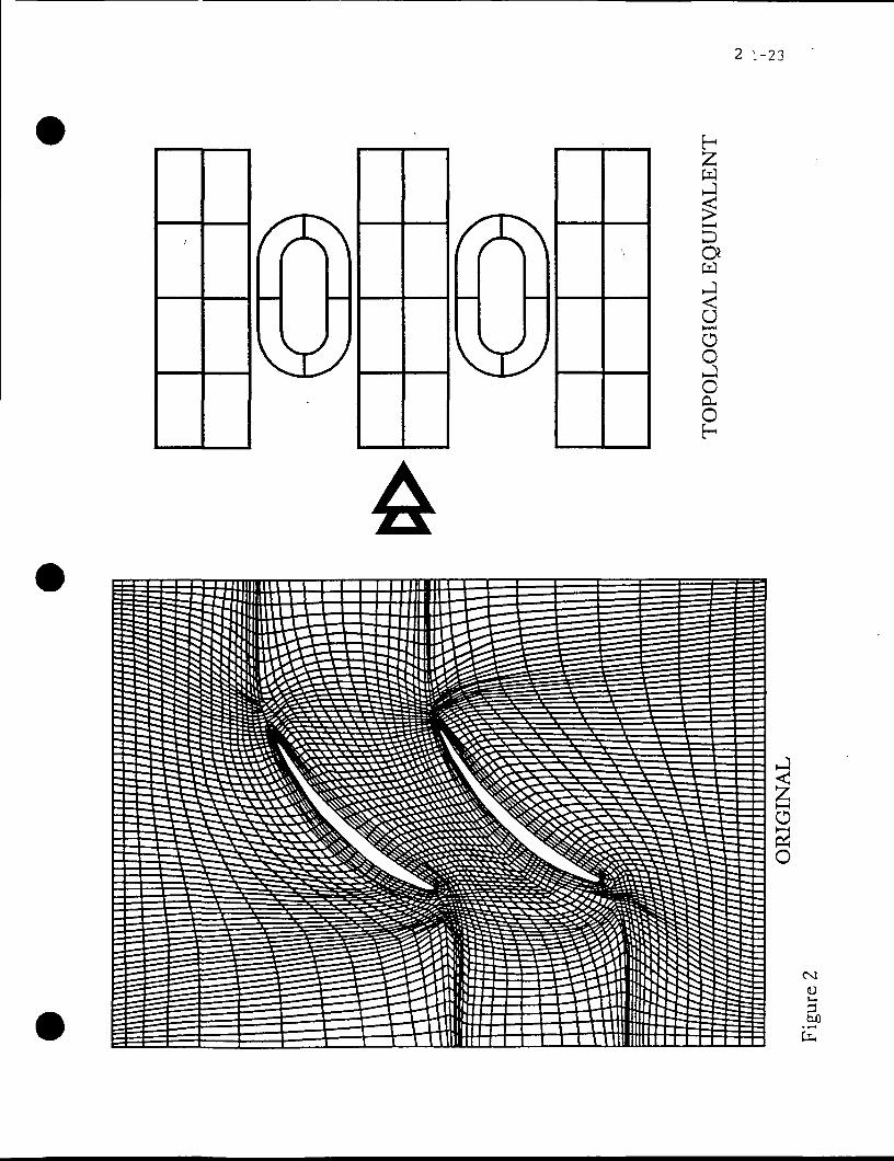
2 ;-23

H2wgI-H

DOWJ<u)—H

OoJoa,Oh

<Nt

W)

2 . - 2 4

Figure 3

2 -25

Root Level Node Row

Unit Cell

[UpstreamI Node Row

( DownstreamI Node Row

Figure 4

2 -26

2nd Level N '

ffl3rd

ffl

4th

Figure 5

2 - 2 7

Figure 6

2-28

Figure 7

2 -29

CO

ol_>

2. -30

f-

'* ' 00

2.-31

Figure 10

2-33

PRECEDING PAGE BLANK NOT FILMEp

_ o

W)

fa

2-34

CMi—i

<Di—

Si

2-35

Figure 13

2-36

Table Captions

Table 1 Charleston Harbor Model: Sequential Speedup

Table 2 Four Turbine Blade Model: Sequential Speedup

Table 1

2-37

Model/Nodes

small2207

medium8036

large18081

Two Level Tree

EffortSpeedup

1.80

2.51

2.50

MemoryReduction

1.30

1.60

1.72

Three Level Tree

EffortSpeedup

2.95

4.25

5.31

MemoryReduction

1.43

1.93

2.37

Table 2

Three Level Tree, nodes = 19718

Partitions/Levels2 3

12124848

256425

100

EffortSpeedup

11.5312.5012.9713.13

MemoryReduction

3.423.563.753.60

Four Level Tree

Partitions/Levels2 3 4

34

1212

25121620

64252520

EffortSpeedup

13.169.44

17.5910.23

MemoryReduction

3.613.203.853.17