final report on design checks for timber decks on steel ... final report on design checks for timber...

1

Final report on design checks for timber decks on steel girders on forestry roads of British Columbia Baidar Bakht Aftab Mufti Gamil Tadros Submitted to Mr. Brian Chow Ministry of Forests and Range British Columbia JMBT Structures Research Inc. 21 Whiteleaf Crescent Scarborough ON M1V 3G1 November 19, 2008

2

Table of contents Executive summary, 3 1. Development of design loading, 5 1.1 Background, 5 1.2. Methodology, 7 1.3. Heavy off-highway design truck, 8 1.4. Light off-highway design truck, 9 1.5. Highway design truck (BCL-625), 11 1.6. Distance between lines of wheels, 12 1.7. Final selection of design trucks, 15 1.7.1 Heavy Off-highway Truck, 15 1.7.2 Light Off-highway Truck, 19 1.7.3 BCL-625 Truck, 21 2. Dispersion of wheel loads through planks, 22 2.1. An extensive exercise, 22 2.2 Effective plank thickness, 22 2.5. Conclusions, 23 3. Design criteria and calculation of properties, 23 3.1. Design criteria, 23 3.1.1 Flexural resistance, 23 3.1.2 Shear resistance, 23 3.1.3 Maximum deflection, 23 3.2. Details of decks, 23 3.3 Calculation of section moduli, 27 3.4 Calculation of factored resistance, 30 3.5 Transverse position of design loading, 33 4. Design checks, 42 4.1 Introduction, 35 4.2 BCL-625 design loading, 35 4.3 Design checks with proposed loadings, 40 4.3.1 Design checks for external ties with original design, 40 4.3.2 Design checks for internal ties with original design, 44 4.3.3 Design checks for external ties with revised design, 49 5. Conclusions, 50 6. Proposal for future work, 51 6.1 Verification of designs by lab tests, 51 6.2 Verification of method of analysis, 53 6.3 Failure of one component, 54 6.4 Conservative values of specified strengths, 54 7. References, 55 Appendix 0. Advice from Buckland & Taylor Ltd. re. Design categories of surveyed vehicles, 56 Appendix 20. Dispersion of wheel loads through planks, 58

3

Executive summary Development of design loading The following configurations are proposed for design loadings for timber decks on steel girder bridge of forestry roads in British Columbia.

The above design loadings are to be used with the following conditions for analyzing the timber decks.

• The live load factor should be 1.7. • The dynamic load allowance should be 0.21. • The wheel loads on cantilever overhangs of the ties should not be used to reduce positive

moments in the ties due to loads between the girders. Dispersion of wheel loads through planks

• Contrary to conventional wisdom, the length of a wheel dispersed through planks in the longitudinal direction of the bridge is relatively insensitive to the thickness or properties of the timber planks.

• For all analyses to be conducted for the design check of timber decks, the individual two rectangular patch loads of a dual-tire are recommended to be idealized as a single point load placed at the CG of the two patch loads.

• For idealizing the timber decks under consideration for the semi-continuum method, the effective thickness of the planking should be taken as twice the actual thickness.

Design criteria and calculation of properties

Distribution of wheel loads on axle

114 114 kN

1.37 m 1.80 m

BCL-625 Loading

50:50

60:40

60:40

161 161 kN

1.37 m 1.90 m

Light Off-highway Loading

280 280 kN

1.80 m 2.50 m

Heavy Off-highway Loading

4

• Consideration of the composite action between the planking and the ties, usually ignored, can increase the flexural resistance of ties by 3 to 18%.

• Consideration of the composite action between the planking and the ties has little effect of the shear capacity of ties.

• The transverse positions of the three proposed design vehicles on timber decks over girders spaced at 3.0 and 3.6 m are shown in Fig. 3.2 (a) and (b), respectively, along with the axle loads, and the relevant vehicle edge distances.

Design checks The conclusions from the design-check exercise for the 48 original deck designs are summarized in the following table with respect to the three proposed design loadings applied with the live load factors of 1.7 and 1.42. Table Outcome of design-check exercise for original designs of the timber decks Design loading

Live load factor

Girder spacing, m

External ties Internal ties

Heavy Off- highway

1.7 3.0 All fail in moment, deflection and shear

All fail in moment, deflection and shear3.6

1.42 3.0 3.6

Light Off- highway

1.7 3.0 All but 1 fail in moment; all but 7 fail in deflection; all fail in shear

All but 8 fail; most failures in moment and shear

3.6 All fail in moment, deflection and shear

All fail, mostly in moment and shear

1.42 3.0 All but 3 fail in moment; all but 9 fail in deflection; all but 2 fail in shear

Slightly more than half fail; most failures in moment and shear



BCL-625 1.7 3.0 All but 8 fail; most failures in moment and shear

Less than half fail in moment and shear

3.6 All but 6 fail; most failures in moment and shear


1.42 3.0 More than half fail; most failures in moment and shear

All meet design requirements

3.6 More than half fail; most failures in moment and shear


The revised design, in which two side-by-side ties are used as an external tie unit, improved the situation only marginally.

5

1. Development of design loading 1.1 Background As discussed in the proposal by JMBT Structures Research Inc., dated July 3, 2007, made to the BC Ministry of Forests and Range (MFR), the current design loads, which were developed from consideration of only longitudinal moments and shears, might not be suitable for determining transverse moments in timber decks on steel girders. It is noted that the MFR has specified three design loadings: (1) BCL-625 Truck (Fig. 1.1), a modified form of the CL-625 Design Truck of CAN/CSA-S6-06 (S6); (2) Light Off-highway Design Truck, shown in Fig. 1.2; and (3) Heavy Off-highway Design Truck, shown in Fig. 1.3. For BCL-625 Truck, the distance V varies between 6.6 and 18.0 m, and the transverse distance between the centrelines of wheels is 1.80 m.

Figure 1.1. BCL-625 Truck (GVW 625 kN)

Figure 1.2. Light Off-highway Design Truck with GVW = 720kN

Figure 1.3. Heavy Off-highway Design Truck (GVW 1120 kN)

assumed 1900

assumed 2500

6

Following a tele-conference on December 3, 2007, with MFR personnel and engineers from Buckland & Taylor Ltd. and Associated Engineering, the distances between the centres of lines of wheels of Light and Heavy Off-highway Trucks were assumed to be 1900 and 2500 mm, respectively (Figs. 1.2 and 1.3). The design loadings for the timber decks were required by the MFR to be developed with the following constraints.

• The loads on the two wheels of an axle of the Heavy and Light Off-highway Trucks should be

divided in the 60:40 ratio, as specified in the MFR design guidelines.

• The loads on the two wheels of axles of BCL-625 Truck should be divided in the 50:50 ratio as specified in S6.

• While the design loading for the timber decks are to be developed from maximum observed loads in the actual survey data, the live load factor should be the same as that specified in S6, i.e. 1.7.

It is recalled that the design live loading for the Ontario Highway Bridge Design Code (OHBDC, 1992) was based on ‘maximum observed loads’, and its live load factor was 1.4. The design live loading for S6 is based on maximum legal loads, and is lighter than the OHBDC design live loading; the live load factor for S6 loading is 1.7. However, the products of the design loads specified by the two codes and the respective live load factors, i.e. the factored loads, are very nearly the same. Both the OHBDC and S6 design trucks have the same base length of 18 m. The total weight of the OHBDC design truck is 740 kN and the live load factor is 1.4, which gives the factored live load = 1036 kN. The factored live load corresponding to the CL-625 Truck is 1062 kN, being only about 2.5% heavier.

The various terms used in conjunction with the development of design live loading for the timber decks, are illustrated in Fig. 1.4. The design loading for timber decks is expected to comprise a number of closely spaced axles. Figure 1.4 shows only two axles; however, three closely spaced axles are also considered in the study.

Figure 1.4. A group of two closely spaced axles

Line of wheels

Wheel R

Distance between lines of wheels

Wheel L

Axle

Direction of travel

Inter-axle spacing

7

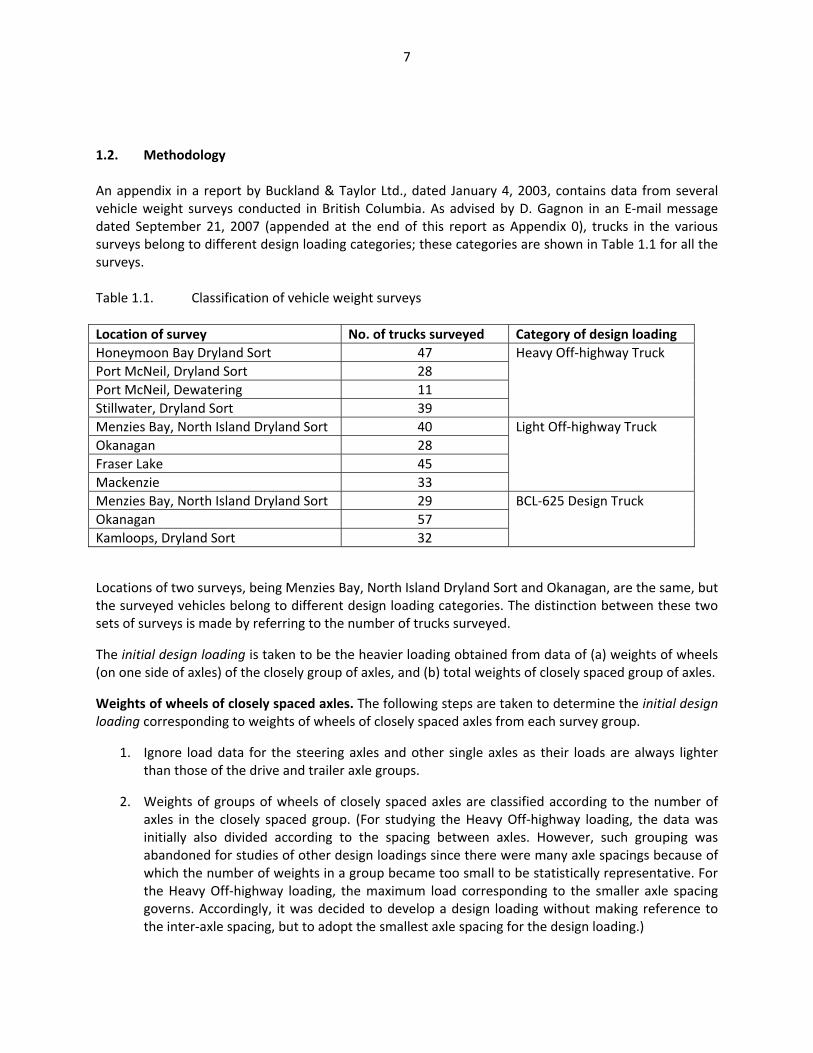
1.2. Methodology An appendix in a report by Buckland & Taylor Ltd., dated January 4, 2003, contains data from several vehicle weight surveys conducted in British Columbia. As advised by D. Gagnon in an E-mail message dated September 21, 2007 (appended at the end of this report as Appendix 0), trucks in the various surveys belong to different design loading categories; these categories are shown in Table 1.1 for all the surveys. Table 1.1. Classification of vehicle weight surveys Location of survey No. of trucks surveyed Category of design loading Honeymoon Bay Dryland Sort 47 Heavy Off-highway Truck Port McNeil, Dryland Sort 28 Port McNeil, Dewatering 11 Stillwater, Dryland Sort 39 Menzies Bay, North Island Dryland Sort 40 Light Off-highway Truck Okanagan 28 Fraser Lake 45 Mackenzie 33 Menzies Bay, North Island Dryland Sort 29 BCL-625 Design Truck Okanagan 57 Kamloops, Dryland Sort 32

Locations of two surveys, being Menzies Bay, North Island Dryland Sort and Okanagan, are the same, but the surveyed vehicles belong to different design loading categories. The distinction between these two sets of surveys is made by referring to the number of trucks surveyed.

The initial design loading is taken to be the heavier loading obtained from data of (a) weights of wheels (on one side of axles) of the closely group of axles, and (b) total weights of closely spaced group of axles.

Weights of wheels of closely spaced axles. The following steps are taken to determine the initial design loading corresponding to weights of wheels of closely spaced axles from each survey group.

1. Ignore load data for the steering axles and other single axles as their loads are always lighter than those of the drive and trailer axle groups.

2. Weights of groups of wheels of closely spaced axles are classified according to the number of axles in the closely spaced group. (For studying the Heavy Off-highway loading, the data was initially also divided according to the spacing between axles. However, such grouping was abandoned for studies of other design loadings since there were many axle spacings because of which the number of weights in a group became too small to be statistically representative. For the Heavy Off-highway loading, the maximum load corresponding to the smaller axle spacing governs. Accordingly, it was decided to develop a design loading without making reference to the inter-axle spacing, but to adopt the smallest axle spacing for the design loading.)

8

3. For each group of weights of wheels of closely spaced axles, calculate the mean (Wmean), maximum (Wmax), minimum (Wmin) and standard deviation (Wsd).

4. For each group of weights of wheels, take the larger of (Wmax) and (Wmean +1.7Wsd) as the maximum weight of the wheels in a group of closely spaced axles. In most cases, (Wmean

+1.7Wsd), representing a confidence limit of about 95%, is slightly larger than Wmax.

5. Divide the larger of (Wmax) and (Wmean +1.7Wsd) by 0.6 to obtain the total maximum observed weight of closely spaced group of axles under consideration; this total weight is the maximum observed load, and accordingly corresponds to the OHBDC (1992) live load factor of 1.4.

6. To obtain the total maximum load of the closely spaced groups with the S6 live load factor of 1.7, multiply the load obtained in Step 5 with (1.4/1.7). The total load obtained in this step is referred to as the ‘initial design load’ for the group of closely spaced axles under consideration.

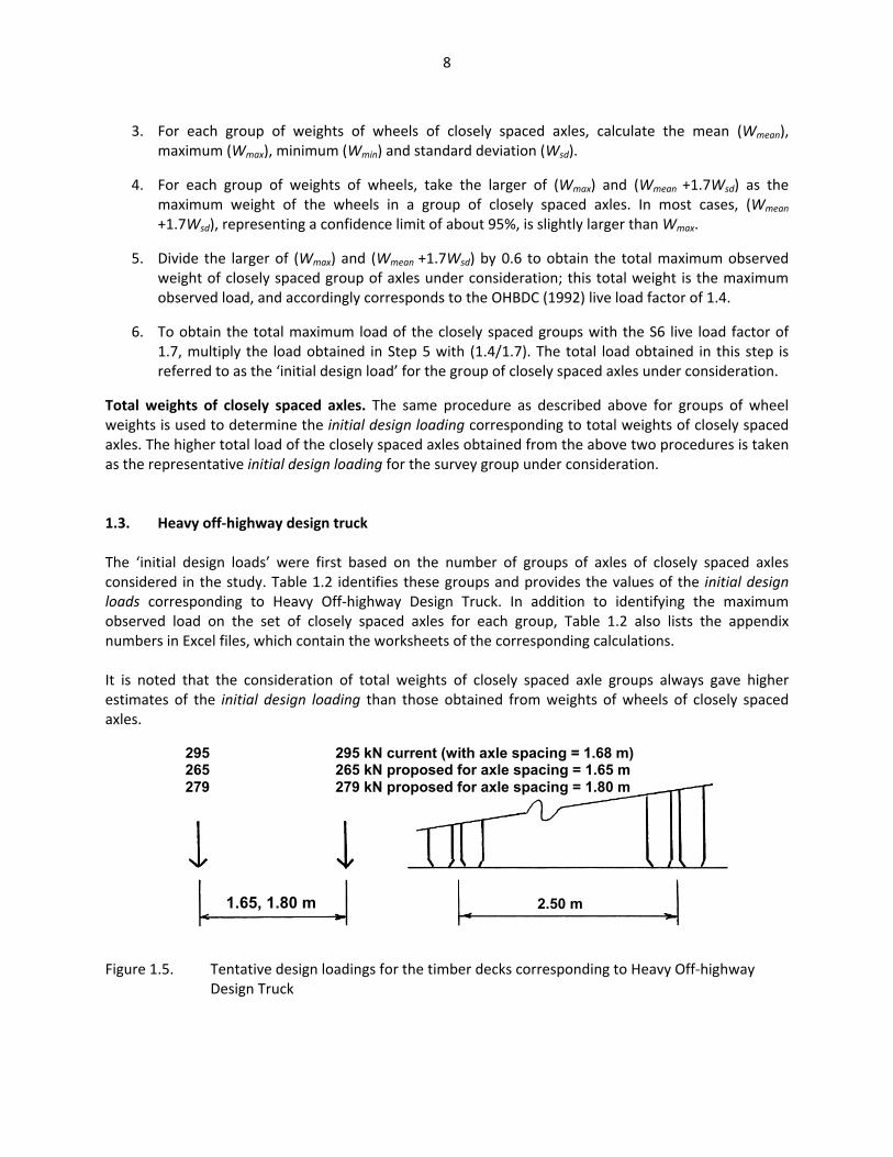
Total weights of closely spaced axles. The same procedure as described above for groups of wheel weights is used to determine the initial design loading corresponding to total weights of closely spaced axles. The higher total load of the closely spaced axles obtained from the above two procedures is taken as the representative initial design loading for the survey group under consideration. 1.3. Heavy off-highway design truck The ‘initial design loads’ were first based on the number of groups of axles of closely spaced axles considered in the study. Table 1.2 identifies these groups and provides the values of the initial design loads corresponding to Heavy Off-highway Design Truck. In addition to identifying the maximum observed load on the set of closely spaced axles for each group, Table 1.2 also lists the appendix numbers in Excel files, which contain the worksheets of the corresponding calculations. It is noted that the consideration of total weights of closely spaced axle groups always gave higher estimates of the initial design loading than those obtained from weights of wheels of closely spaced axles.

Figure 1.5. Tentative design loadings for the timber decks corresponding to Heavy Off-highway Design Truck

1.65, 1.80 m

295 295 kN current (with axle spacing = 1.68 m) 265 265 kN proposed for axle spacing = 1.65 m 279 279 kN proposed for axle spacing = 1.80 m

2.50 m

9

From the results presented in Table 1.2, it is intuitively obvious that the final design loading is represented by a 2-axle group with an inter-axle spacing of either 1.65 m, or 1.80 m, both from survey at Port McNeil Dewatering. (If the total load on two axles = 527 kN, assuming equal distribution of load on the two axles, the weight on each axle = 265 kN). However, the intuitive observation has to be confirmed by analyzing a wood deck with worst possible load distribution characteristics under the two loadings identified above. As shown in Fig. 1.5, one of the tentative design axle groups has nearly the same inter-axle spacing as that of Heavy Off-highway Design Truck (Fig. 1.3), but its loads are lighter by about 10% than those of the first 2-axle group of design vehicle of Fig. 1.2. The distance between the lines of wheels can also be a factor in determining the design loading; this aspect is dealt with in Section 1.6. Table 1.2. Initial design weights of closely spaced axles corresponding to Heavy Off-highway Truck

Survey location

No. of axles

Inter-axle spacing,

m

Total ‘initial design

weight’ of closely spaced

axles, kN

Spacing between two

lines of wheels, m

Maximum observed load on one set of wheels on closely spaced

axles, kN

Worksheet in

Appendix

Honeymoon Bay Dryland

2 1.65 477 2.53 307 1

2 1.80 547 2.53 345 2

Port McNeil Dryland

2 1.69 441 2.54 277 3

Port McNeil Dewatering

2 1.65 527 2.53 377 4

2 1.80 557 2.53 359 5

Stillwater Dryland

2 1.37 316 2.05 208 6

3 1.37 391 2.05 285 7

It is noted that the 3-axle group need not be considered further for the Heavy Off-highway Design Truck because its maximum total weight of 391 kN spread over 2.74 m (391 kN) is significantly lighter than the 527 kN weight of the lighter of the 2-axle groups from the survey of Port McNeil Dewatering. 1.4. Light off-highway design truck For vehicle surveys corresponding to the category of Light Off-highway Design loading, the calculations can be found in Appendices 8 through 14, and the initial design weights of closely spaced axle groups are listed in Table 1.3.

10

The three closely spaced groups of axles having the maximum weights in their categories (corresponding to the number of axles) are highlighted in Table 1.3, and illustrated in Fig. 1.6. It can be seen in this figure that the initial design weight of the 2-axle group is about 20% lighter than that of 2-axle groups of the Light Off-highway Design Truck of Fig. 1.2. The final design loading for the loading category under consideration will be selected after analyzing the timber deck with worst load distribution characteristics. Table 1.3. Initial design weights of closely spaced axles corresponding to Light Off-highway Truck

Survey location

No. of axles

Inter-axle spacing,

m



axles, kN

Spacing between two

lines of wheels, m


axles, kN

Worksheet in

Appendix No.

Menzies Bay, N. Island

Dryland Sort

3 1.4 259 2.01 175 8

Okanagan Falls

3 1.37-1.42 303 2.04 189 9

2 1.37-1.42 257 2.04 164 10

Mackenzie 3 1.21-1.40 294 2.05 211 11

3 1.64-1.80 357 2.05 215 11

2 1.37-1.39 321 2.05 203 12

Fraser Lake 3 1.37-1.42 340 1.89-2.05 208 13

2 1.37-1.41 316 1.89-2.05 200 14

11

Figure 1.6. Tentative design loadings for the timber decks corresponding to Light Off-highway Design Truck: (a) 2-axle group, (b) 3-axle group with inter-axle spacing of 1.37 m, (c) 3-axle group with spacing of 1.64 m 1.5. Highway design truck (BCL-625) For vehicle surveys corresponding to the category of highway vehicles, i.e. BCL-625 Design loading, the calculations can be found in Appendices 15 through 20, and the initial design weights of closely spaced axle groups are listed in Table 1.4.

Figure 1.7. Tentative design loadings for the timber decks corresponding to highway (CL-625) Design Truck: (a) 2-axle group, and (b) 3-axle group

The ‘initial design loadings’ calculated from surveys of highway vehicles for 2- and 3-axle groups are shown in Fig. 1.7, along with the details of the corresponding 2-axle group of BCL-625 Design Truck. Since the 2-axle loads of the BCL-625 Design Truck are heavier and have smaller inter-axle spacing than those of the ‘design loading’ calculated from the survey data, it is obvious that BCL-625 loading will

205 205 kN current (with axle spacing = 1.68 m) 161 161 kN proposed 113 113 113 kN

1.37 m 1.37 m 1.37 m

(a) (b)

proposed 119 119 119 kN

1.64 m 1.64 m

(c)

140 140 kN BCL-625 (with axle spacing = 1.20 m)

114 114 kN from survey 83 83 83 kN

1.37 m from survey 1.37 m 1.37 m

1.20 m BCL-625

(b) (b)

12

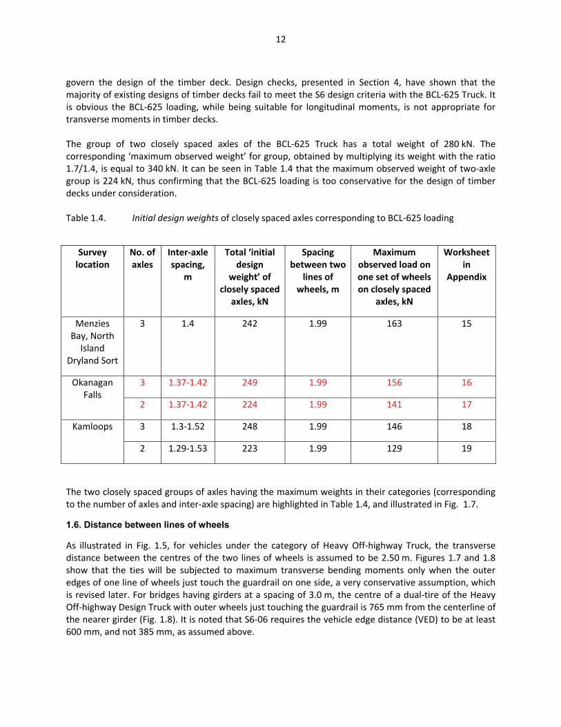
govern the design of the timber deck. Design checks, presented in Section 4, have shown that the majority of existing designs of timber decks fail to meet the S6 design criteria with the BCL-625 Truck. It is obvious the BCL-625 loading, while being suitable for longitudinal moments, is not appropriate for transverse moments in timber decks. The group of two closely spaced axles of the BCL-625 Truck has a total weight of 280 kN. The corresponding ‘maximum observed weight’ for group, obtained by multiplying its weight with the ratio 1.7/1.4, is equal to 340 kN. It can be seen in Table 1.4 that the maximum observed weight of two-axle group is 224 kN, thus confirming that the BCL-625 loading is too conservative for the design of timber decks under consideration. Table 1.4. Initial design weights of closely spaced axles corresponding to BCL-625 loading

Survey location

No. of axles

Inter-axle spacing,

m



axles, kN

Spacing between two

lines of wheels, m


axles, kN

Worksheet in

Appendix

Menzies Bay, North

Island Dryland Sort

3 1.4 242 1.99 163 15

Okanagan Falls

3 1.37-1.42 249 1.99 156 16

2 1.37-1.42 224 1.99 141 17

Kamloops 3 1.3-1.52 248 1.99 146 18

2 1.29-1.53 223 1.99 129 19

The two closely spaced groups of axles having the maximum weights in their categories (corresponding to the number of axles and inter-axle spacing) are highlighted in Table 1.4, and illustrated in Fig. 1.7.

1.6. Distance between lines of wheels

As illustrated in Fig. 1.5, for vehicles under the category of Heavy Off-highway Truck, the transverse distance between the centres of the two lines of wheels is assumed to be 2.50 m. Figures 1.7 and 1.8 show that the ties will be subjected to maximum transverse bending moments only when the outer edges of one line of wheels just touch the guardrail on one side, a very conservative assumption, which is revised later. For bridges having girders at a spacing of 3.0 m, the centre of a dual-tire of the Heavy Off-highway Design Truck with outer wheels just touching the guardrail is 765 mm from the centerline of the nearer girder (Fig. 1.8). It is noted that S6-06 requires the vehicle edge distance (VED) to be at least 600 mm, and not 385 mm, as assumed above.

13

In Clause 3.8.4.3, S6 does require the minimum distance from the centres of the wheels to the curb, railing or barrier wall to be 0.30 m. However, this clause pertains to ‘local components’, being ‘components of deck plate and grid systems’, for which the load effects increase rapidly as the wheels approach curb or barrier (Clause C3.8.4.3 of S6.1-06). For the ties under consideration, the locations of maximum moments or shears are well away from the curb or barrier. Consequently, Clause 3.8.4.3 is not applicable for the timber ties under consideration.

Figure 1.8. Transverse position of Heavy Off-highway Design Truck on timber deck on girders at a spacing of 3.0 m For bridges having girders at a spacing of 3.6 m, the centre of a dual-tire of the Heavy Off-highway Design Truck with outer wheels just touching the guardrail is 1335 mm from the centerline of the nearer girder (Fig. 1.9). It is noted that for purposes of analysis, a dual tire is represented as a point load in the transverse direction of the bridge.

770 770

385 2530 735

650 3000 650

3300 770 770

385 2500 765

Planks Ties

650 3000 650

3300

770 770

Dual-tire represented as point load

14

Figure 1.9. Transverse position of Heavy Off-highway Design Truck on timber deck on girders at a spacing of 3.6 m

Figure 1.10. Transverse position of Light Off-highway Design Truck on timber deck on girders at a spacing of 3.0 m

770 770

385 2500 1365

650 3600 650

Dual tire represented as point load

650 3000 650

770 770

385 1900 1365

Dual tire represented as point load

15

For the Light Off-highway Design Truck, the transverse distance between the two lines of wheels varies between 1.89 and 2.05 m (see Table 1.3). A conservative value of 1.90 m for the spacing between the two lines of wheels was endorsed at the tele-conference on October 29, 2007 (Bakht, Chow, Gagnon, Henley, McClelland, and Penner). As illustrated in Fig. 1.10, for maximum transverse bending moments due to the Light Off-highway Design Truck in ties on girders spaced at 3.0 m, one line of wheels of design truck is placed transversely 1,365 mm away from the centerline of the nearer girder. For timber decks of girders spaced at 3.6 m, the ties are subjected to maximum transverse moments when one line of wheels of the Light Off-highway Design Truck is midway between the two girders. As illustrated in Fig. 1.11, for this loading the other line of wheels does not touch the guard rail.

Figure 1.11. Transverse position of Light Off-highway Design Truck on timber deck on girders at a spacing of 3.6 m

1.7. Final selection of design trucks

1.7.1 Heavy Off-highway Truck

As illustrated in Fig. 1.5, two 2-axle configurations are initially proposed for the design loading corresponding to the Heavy Off-highway loading. Each of these configurations is composed of two axles. In one configuration, designated as Loading A, the axle load and inter-axle spacing are 265 kN and 1.65 m, respectively; in the other configuration (Loading B), the corresponding values are 279 kN and

770 770

650 1900 1700

650 3600 650

16

1.8 m, respectively. The configuration, giving higher transverse moment in the timber ties of a deck having the worst load distribution characteristics, will be selected as the final loading. For worst load distribution characteristics, the deck should have (a) the smallest span, (b) ties with the largest flexural rigidity, and (c) thinnest planking. Accordingly, a deck with following properties is chosen for the exercise at hand. Girder spacing 3000 mm Cross-section of tie 250×300 mm Spacing of ties 406 mm Species of ties Select structural Douglas fir-larch E50 of ties 12,000 MPa Thickness of planks 100 mm Species of planks Grade No. 2, Northern species E50 of planks 6,300 MPa As specified in Clause 3.8.4.5.3 (c) of S6, the basic dynamic load allowance (DLA) for two axles is 0.30. For wood components, this DLA is multiplied by 0.7 (Clause 3.8.4.5.4), giving the final DLA for two closely spaced axles = 0.21. Using live load factor, αL, of 1.7, for Loading A, the factored maximum wheel load = 0.6×1.7×(1.00+0.21) ×265 = 327 kN Similarly, for Loading B, the factored maximum wheel load = 0.6×1.7×(1.00+0.21) ×280 = 346 kN For the analysis under consideration, each wheel load was represented by two half-wheels at a spacing of 0.4 m in the longitudinal direction of the bridge. Hence the factored half-wheels for Loadings A and B are 164 and 173 kN, respectively. As shown in Section 2, rigorous analysis showed that the representation of a single wheel load by two point loads is not realistic for load dispersion of patch loads through timber planks. Accordingly, analyses discussed in later sections were performed by representing each wheel load by a point load. It is important to note, however, that the representation of a wheel load by two point loads for the comparative exercise under consideration is not expected to change the outcome because the same representation was used for both analyses. The timber deck with worst load distribution characteristic (described above) was analyzed under the two set of factored half-wheels by SECAN (Mufti et al., 2003), which is based on the semi-continuum method (Jaeger and Bakht, 1989). The idealized deck is shown in Fig. 1.12 in plan without the planking.

17

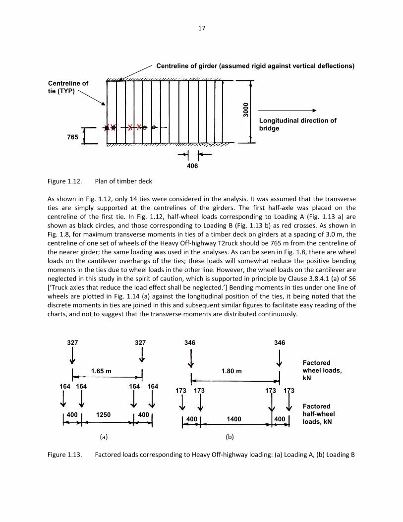
Figure 1.12. Plan of timber deck As shown in Fig. 1.12, only 14 ties were considered in the analysis. It was assumed that the transverse ties are simply supported at the centrelines of the girders. The first half-axle was placed on the centreline of the first tie. In Fig. 1.12, half-wheel loads corresponding to Loading A (Fig. 1.13 a) are shown as black circles, and those corresponding to Loading B (Fig. 1.13 b) as red crosses. As shown in Fig. 1.8, for maximum transverse moments in ties of a timber deck on girders at a spacing of 3.0 m, the centreline of one set of wheels of the Heavy Off-highway T2ruck should be 765 m from the centreline of the nearer girder; the same loading was used in the analyses. As can be seen in Fig. 1.8, there are wheel loads on the cantilever overhangs of the ties; these loads will somewhat reduce the positive bending moments in the ties due to wheel loads in the other line. However, the wheel loads on the cantilever are neglected in this study in the spirit of caution, which is supported in principle by Clause 3.8.4.1 (a) of S6 [‘Truck axles that reduce the load effect shall be neglected.’] Bending moments in ties under one line of wheels are plotted in Fig. 1.14 (a) against the longitudinal position of the ties, it being noted that the discrete moments in ties are joined in this and subsequent similar figures to facilitate easy reading of the charts, and not to suggest that the transverse moments are distributed continuously.

(a) (b) Figure 1.13. Factored loads corresponding to Heavy Off-highway loading: (a) Loading A, (b) Loading B

765

3000

406

Centreline of girder (assumed rigid against vertical deflections)

Centreline of tie (TYP)

Factored wheel loads, kN

Factored half-wheel loads, kN

327 327 346 346

1.65 m 1.80 m

164 164 164 164

400 1250 400

173 173 173 173

400 1400 400

Longitudinal direction of bridge

18

In Fig. 1.14 (a), it can be seen that Loading B gives slightly higher bending moment in the external tie than the moment due to Loading A. Accordingly, Loading B is selected as the Heavy Off-highway Design loading for the timber decks; details of this design loading, without the live load factor and DLA, are given in Fig. 1.15.

(a) (b) Figure 1.14. Bending moments in ties due to half-wheel loads of Fig. 1.13: (a) deck with worst load distribution characteristics, (b) deck with best load distribution characteristics To confirm that the selected loading gives higher tie moments even in decks with the best load distribution characteristics, a deck having ties with the smallest flexural rigidity and thickest planks was analyzed under the same two initial design loadings as were used for the deck with the worst load distribution characteristics. The results, plotted in Fig. 1.14 (b), confirm that the selected loading gives very nearly the same maximum tie moments in the deck with the best load distribution characteristics as the other loading. The charts given in Fig. 1.14 confirm that the load distribution characteristics of the deck have only marginal effect on the selection of the design load for the deck; this observation is useful in concluding that the design loading selected mainly for timber decks should also remain valid for concrete deck slab and steel grating, the former of which has much better distribution characteristics than the timber deck.

1.80

Loading A

Loading B

Ben

ding

mom

ent i

n tie

s, k

N.m

125

100

75

50

25

0 Longitudinal position of tie

Loading B (TYP)

Loading A (TYP)

19

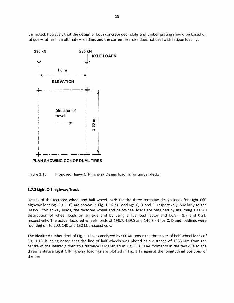
It is noted, however, that the design of both concrete deck slabs and timber grating should be based on fatigue – rather than ultimate – loading, and the current exercise does not deal with fatigue loading.

Figure 1.15. Proposed Heavy Off-highway Design loading for timber decks 1.7.2 Light Off-highway Truck Details of the factored wheel and half wheel loads for the three tentative design loads for Light Off-highway loading (Fig. 1.6) are shown in Fig. 1.16 as Loadings C, D and E, respectively. Similarly to the Heavy Off-highway loads, the factored wheel and half-wheel loads are obtained by assuming a 60:40 distribution of wheel loads on an axle and by using a live load factor and DLA = 1.7 and 0.21, respectively. The actual factored wheels loads of 198.7, 139.5 and 146.9 kN for C, D and loadings were rounded off to 200, 140 and 150 kN, respectively. The idealized timber deck of Fig. 1.12 was analyzed by SECAN under the three sets of half-wheel loads of Fig. 1.16, it being noted that the line of half-wheels was placed at a distance of 1365 mm from the centre of the nearer girder; this distance is identified in Fig. 1.10. The moments in the ties due to the three tentative Light Off-highway loadings are plotted in Fig. 1.17 against the longitudinal positions of the ties.

280 kN 280 kN

1.8 m

AXLE LOADS

ELEVATION

PLAN SHOWING CGs OF DUAL TIRES

2.50

m

Direction of travel

20

Figure 1.16. Factored wheel and half-wheel loads for tentative design loadings for Light Off-highway loading: (a) Loading C, (b) Loading D, (c) Loading E (Note: representation of a wheel load by two point loads is abandoned in subsequent sections)

Figure 1.17. Bending moments in ties due to factored half-wheel loads of Fig. 1.16

FACTORED WHEEL LOADS, kN

FACTORED HALF-WHEEL LOADS, kN





200 200

1.37 m

100 100 100 100

0.4 0.97 0.4 m

(a)

140 140 140

1.37 1.37 m 70 70 70 70 70 70

0.4 1.37 0.4 1.37 0.4

(b)

150 150 150

1.64 1.64 75 75 75 75 75 75

(c)

Loading E

Loading D

Loading C

Ben

ding

mom

ent i

n tie

s, k

N.m

75

50

25

0

Longitudinal position of tie

Loading C

Loading D

Loading E

0.4

21

It can be seen in Fig. 1.17 that the 2-axle loading, i.e. Loading C, gives the highest moment in the ties. Accordingly, this loading is chosen as the final Light Off-highway design load for the timber decks under consideration; details of this design loading, without the live load factor and DLA, are given in Fig. 1.18.

Figure 1.18. Proposed Light Off-highway Design loading for timber decks 1.7.3 BCL-625 Truck It can be readily concluded from Fig. 1.7 that the governing load configuration corresponding to BCL-625 load is the two-axle group; this configuration is illustrated in Fig. 1.19.

161 kN 161 kN

1.37 m

AXLE LOADS

ELEVATION


1.90

m

Direction of travel

22

Figure 1.19. Proposed BCL-625 loading for timber decks 2. Dispersion of wheel loads through planks 2.1 An extensive exercise It was initially postulated that the thickness of timber planks has a significant effect not only on the load distribution characteristics of the deck but also on the size of the effective contact area of a wheel load that is transferred to the ties. To confirm the latter postulate, an extensive analytical exercise was undertaken to determine quantitatively the effect of load dispersion through the timber planking. The analytical exercise, however, showed that the size of the wheel load dispersed through the timber planking is not affected significantly by the thickness of the planking. Details of the analytical study are included in Appendix A20 for records. 2.2 Effective plank thickness Cheung et al. (1982) have dealt with the analysis of box girders by the grillage analogy, in which each girder is represented as a single one-dimensional beam; they concluded that the deck slab flexes between the webs of the box girders, and not between the centrelines of the boxes. Because of this conclusion, Cheung et al. (1982) recommend that the flexibility of the deck slab of the idealized grillage should have a larger thickness than that of the actual deck slab with smaller effective span, so that the flexibilities of the idealized and actual deck slabs are nearly the same.

114 kN 114 kN

1.37 m

ELEVATION

Direction of travel


1.80

m

AXLE LOADS

23

Most of timber deck designs involve ties having nearly the same widths as the clear spacing between the ties, so the spacing of the idealized ties is about twice the clear spacing between the ties. It can be readily shown that for such cases, the effective thickness of the planking of the idealized semi-continuum should be about twice the actual thickness. The design checks, discussed in Section 4 will be conducted by using this assumption. 2.3. Conclusions

The following conclusions are drawn from the analytical study discussed in this section.


• For all analyses to be conducted for the design check of timber decks, the two individual rectangular patch loads of a dual-tire are recommended to be idealized as a single point load placed at the CG of the two patch loads.


3. Design criteria and calculation of properties 3.1. Design criteria 3.1.1 Flexural resistance According to Clause 9.6.1 of S6, the factored flexural resistance, Mr, of a wood component is calculated from: SfkkkkM busbmlsdr φ= (3.1)

where φ, resistance factor for flexure, =0.9 (Clause 9.4.4) kd, load duration factor, = 1.0 (Clause 9.5.3) kls, lateral stability factor, = 1.0 (Clause 9.6.3) km, load sharing factor, depends upon the number of ties sharing the load nearly equally (within 15% of each other). ksb, size effect factor, = 1.17 and 1.08 for 250 and 300 mm deep ties, respectively (for other depths, the factor can be found by interpolation from Fig. 3.1) fbu, the specified bending strength, is obtained from Table 9.13, depending upon the species and Grade of wood. (The distinction between the ‘beam and stringer’ and ‘post and timber’ categories is discussed later)

24

S, the section modulus, = bd2/6

Figure 3.1 Relationship between ksh and larger dimension of cross-section of a timber beam 3.1.2 Shear resistance According to Clause 9.7.1, the factored shear resistance, Vr, of a tie is calculated from: 5.1/AfkkkV vusvmdr φ= (3.2)

where φ, resistance factor for shear, =0.9 (Clause 9.5.4) A, the cross-sectional area, = bd fvu, the specified shear strength, is obtained from Table 9.13, depending upon the species and Grade of wood All other factors are the same as the corresponding factors for flexural resistance. 3.1.3 Maximum deflection According to Clause 9.4.2, the maximum deflection of ties should not exceed 1/400 of the span of the tie under SLS live loads. In calculating the deflections of ties, the mean modulus of elasticity, E50, obtained from Table 9.13 depending upon the species and grade of wood, is to be used. The live load factored to be used for SLS is 0.9. 3.2. Details of decks There are only four combinations of cross-sections and spacing of ties. The properties of the various timber decks, however, change according to the species and Grade of wood. According to MFR drawings, the wood for the ties should always be ‘#2 and BTR Coast D-Fir’. However, with the consent of MFR, it is assumed that the ties can be Grade SS, No. 1 or No. 2 of either Douglas fir-Larch (DFL) or Spruce-Pine-Fir (SPF). The resulting combinations of various deck designs with DFL and SPF ties are listed in Tables 3.1 and 3.2, respectively, along with the relevant basic properties of the timber and ties, depending upon whether the cross-section of the tie is regarded as one belonging to the category of beam and stringer (B&S) or post and timber (P&T).

1.3

1.2

1.1

1.0

ksb

0 100 200 250 300 400

1.17

1.08

Larger dimension of cross-section, mm

25

The division between the categories of B&S and P&T appears somewhat confusing and deserves some clarification. The S6 specifies that timber components should be regarded in the category of B&S when the smaller dimension of the cross-section is at least 114 mm and the larger dimension is more than 51 mm greater than the smaller dimension. When the difference in the two dimensions of the cross-section is less than 51 mm, the component falls in the category of P&T. According to these definitions, the 200×250 and 250×300 mm ties fail to remain in the B&S category by only 1 mm. By putting these ties in the category of P&T, fbu drops by 7, 13 and 33 % for select structural, No. 1 and 2 grades, respectively. At a cursory glance, the division between the two categories of cross-sections on the basis of the difference of only 1 mm in their cross-sectional dimensions appears arbitrary because an accuracy of 1 mm is hard to achieve in the cross-section of a timber component, because of which a designer is likely to feel justified in regarding the 200×250 and 250×300 mm ties in the category of B&S. The difference in the two categories, however, lies not in the dimensional differences of the cross-section, but how the visual grading is done for the two categories. With respect to the edge-knots, the requirements for grading a B&S component are more restrictive than those for a P&T component (NLGA, 2003), because the flexural failure of a B&S component is more affected by the edge-knots than a predominantly compressive failure of P&T component. As recommended by Penner (2008), the two cross-sections of timber components should preferably be defined as follows for purposes of grading.

• Beam and stringer – sawn wood having the two nominal cross-sectional dimensions with a difference of 2 inches (50 mm) or greater.

• Post and timber – sawn wood having the two nominal cross-sectional dimensions with a

difference of 4 inches (100 mm) or greater. It is noted that the above definition, which are consistent with the NLGA standard, should be reviewed carefully with respect to the actual grading rules. In this report, the 200×250 and 250×300 mm ties are considered in the category of B&S. If one of these ties fail to meet the design requirement despite being considered as B&S, then it is obvious that these cross-sections will also fail if they are considered as P&T. Tables 3.1 and 3.2 list the values E50, G50, fbu and fvu for DFL and SPF components, respectively. For 200×250 and 250×300 mm ties, the various properties are given for both B&S and P&T categories, with the properties for the latter being given within brackets. In both Tables 3.1 and 3.2, the mean shear modulus,G50, is calculated by assuming that its value is 0.015×E50 (Clause A5.2.2 of S6). The first layer of planks (plank sub-base) is assumed to be made of 100 mm thick planks of DFL, Grade No. 2, for which S6 specifies E50 to be 9,800 MPa. The mean shear modulus, G50, is calculated to be 147 MPa. The 175 mm thick planks are assumed to be composed of a 100 mm thick plank sub-base of DFL, Grade No. 2, and a 75 mm thick layer of Grade No. 2 Northern species, for which S6 specifies E50 to be 6,300 MPa. Assuming full composite action between the two layers of planks, the effective thickness of the composite planks is found to be 161 mm, in terms of the modulus of elasticity of the plank sub-base.

26

Table 3.1. Details of ties made with DFL Cross-section Designation

of cross-section

I, mm4 J, mm4 Grade E50, MPa G50, MPa fbu, MPa fvu, MPa

X1

260e6 320e6 SS 12,000 (12,000)

180 (180)

19.5 (18.3)

1.5 (1.5)

No. 1 12,000 (10,500)

180 (158)

15.8 (13.8)

1.5 (1.5)

No. 2 9,500 (9,500)

142.5 (142.5)

9.0 (6.0)

1.5 (1.5)

X2

450e6 384e6 SS 12,000 180 19.5 1.5 No. 1 12,000 180 15.8 1.5 No. 2 9,500 142.5 9.0 1.5

X3

562e6 750e6 SS 12,000 (12,000)

180 (180)

19.5 (18.3)

1.5 (1.5)

No. 1 12,000 (10,500)

180 (158)

15.8 (13.8)

1.5 (1.5)

No. 2 9,500 (9,500)

142.5 (142.5)

9.0 (6.0)

1.5 (1.5)

X4

562e6 750e6 SS 12,000 (12,000)

180 (180)

19.5 (18.3)

1.5 (1.5)

No. 1 12,000 (10,500)

180 (158)

15.8 (13.8)

1.5 (1.5)

No. 2 9,500 (9,500)

142.5 (142.5)

9.0 (6.0)

1.5 (1.5)

Note: timber properties given within brackets are for the category of P&T; the other properties are for the category of B&S

27

Table 3.2. Details of ties made with SPF Cross-section Designation

of cross-section

I, mm4 J, mm4 Grade E50, MPa G50, MPa fbu, MPa fvu, MPa

X1

260e6 320e6 SS 8,500 (8,500)

127.5 (127.5)

13.6 (12.7)

1.2 (1.2)

No. 1 8,500 (7,500)

127.5 (112.5)

11.0 (9.6)

1.2 (1.2)

No. 2 6,500 (6,500)

97.5 (97.5)

6.3 (4.2)

1.2 (1.2)

X2

450e6 384e6 SS 8,500 127.5 13.6 1.2 No. 1 8,500 127.5 11.0 1.2 No. 2 6,500 97.5 6.3 1.2

X3

562e6 750e6 SS 8,500 (8,500)

127.5 (127.5)

13.6 (12.7)

1.2 (1.2)

No. 1 8,500 (7,500)

127.5 (112.5)

11.0 (9.6)

1.2 (1.2)

No. 2 6,500 (6,500)

97.5 (97.5)

6.3 (4.2)

1.2 (1.2)

X4

562e6 750e6 SS 8,500 (8,500)

127.5 (127.5)

13.6 (12.7)

1.2 (1.2)

No. 1 8,500 (7,500)

127.5 (112.5)

11.0 (9.6)

1.2 (1.2)

No. 2 6,500 (6,500)

97.5 (97.5)

6.3 (4.2)

1.2 (1.2)

Note: timber properties given within brackets are for the category of P&T; the other properties are for the category of B&S 3.3 Calculation of section moduli Although the planks are secured to the ties by extensive nailing, the composite action between the planks and ties is usually ignored because of the very small modulus of elasticity of the transverse planks in the longitudinal direction of the bridge. However, it was found that the consideration of composite action between the planking and ties can enhance the flexural capacity of the ties noticeably. The section moduli for both non-composite and composite ties of the various decks were calculated by using the spreadsheet software Excel; these moduli are listed in Tables 3.3, 3.4, 3.5 and 3.6 for cross-sections X1, X2, X3 and X4, respectively. It can be seen from these tables that the consideration of composite action increases the value of S for decks with X1 cross-section by 6 to 18%. For decks with X2, X3 and X4 cross-sections, the ranges of this increment drops to 4-14%, 3-12% and 3-9%, respectively.

28

Table 3.3. Section moduli for ties in decks with cross-section X1 (considered in the category of B&S)

Species Grade No. of layers

of planking

S for non-composite tie, mm3

S for composite tie,

mm3

% increase of Sof composite tie over S of

non-composite tie

DFL SS 1 2042717 2164496 6

DFL SS 2 2013496 2259541 11

DFL No. 1 1 2042717 2164496 6

DFL No. 1 2 2013496 2259541 11

DFL No. 2 1 2032290 2185028 7

DFL No. 2 2 1995891 2303127 13

SPF SS 1 2026449 2196477 8

SPF SS 2 1986085 2327262 15

SPF No. 1 1 2026449 2196477 8

SPF No. 1 2 1986085 2327262 15

SPF No. 2 1 2009566 2229354 10

SPF No. 2 2 1957967 2395902 18 Table 3.4. Section moduli for ties in decks with cross-section X2 (considered in the category of B&S)


of planking



mm3


non-composite tie

DFL SS 1 2959144 3091687 4

DFL SS 2 2925663 3183950 8

DFL No. 1 1 2959144 3091687 4

DFL No. 1 2 2925663 3183950 8

DFL No. 2 1 2948577 3115075 5

DFL No. 2 2 2906710 3230021 10

SPF SS 1 2942643 3128150 6

SPF SS 2 2896116 3255628 11

SPF No. 1 1 2942643 3128150 6

SPF No. 1 2 2896116 3255628 11

SPF No. 2 1 2925433 3165831 8

SPF No. 2 2 2865587 3328836 14

29

Table 3.5. Section moduli for ties in decks with cross-section X3 (considered in the category of B&S)


of planking



mm3


non-composite tie

DFL SS 1 3700941 3833921 3

DFL SS 2 3667347 3927196 7

DFL No. 1 1 3700941 3833921 3

DFL No. 1 2 3667347 3927196 7

DFL No. 2 1 3688243 3855435 4

DFL No. 2 2 3646200 3971972 8

SPF SS 1 3681112 3867483 5

SPF SS 2 3634366 3996931 9

SPF No. 1 1 3681112 3867483 5

SPF No. 1 2 3634366 3996931 9

SPF No. 2 1 3660422 3902285 6

SPF No. 2 2 3600210 4068574 12 Table 3.6. Section moduli for ties in decks with cross-section X4 (considered in the category of B&S)


of planking



mm3


non-composite tie

DFL SS 1 3713025 3813368 3

DFL SS 2 3687566 3884175 5

DFL No. 1 1 3713025 3813368 3

DFL No. 1 2 3687566 3884175 5

DFL No. 2 1 3703416 3829718 3

DFL No. 2 2 3671480 3918419 6

SPF SS 1 3698011 3838893 4

SPF SS 2 3662459 3937567 7

SPF No. 1 1 3698011 3838893 4

SPF No. 1 2 3662459 3937567 7

SPF No. 2 1 3682303 3865471 5

SPF No. 2 2 3636341 3992769 9

30

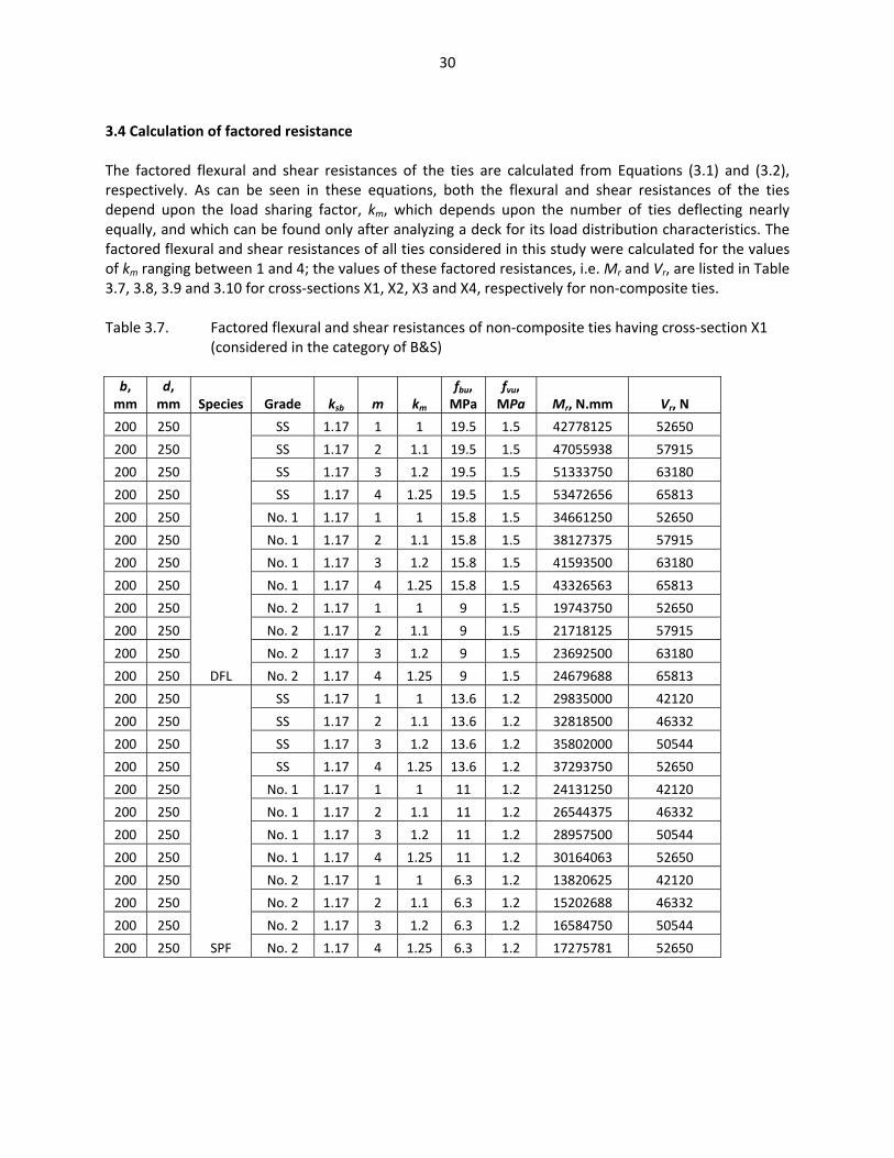
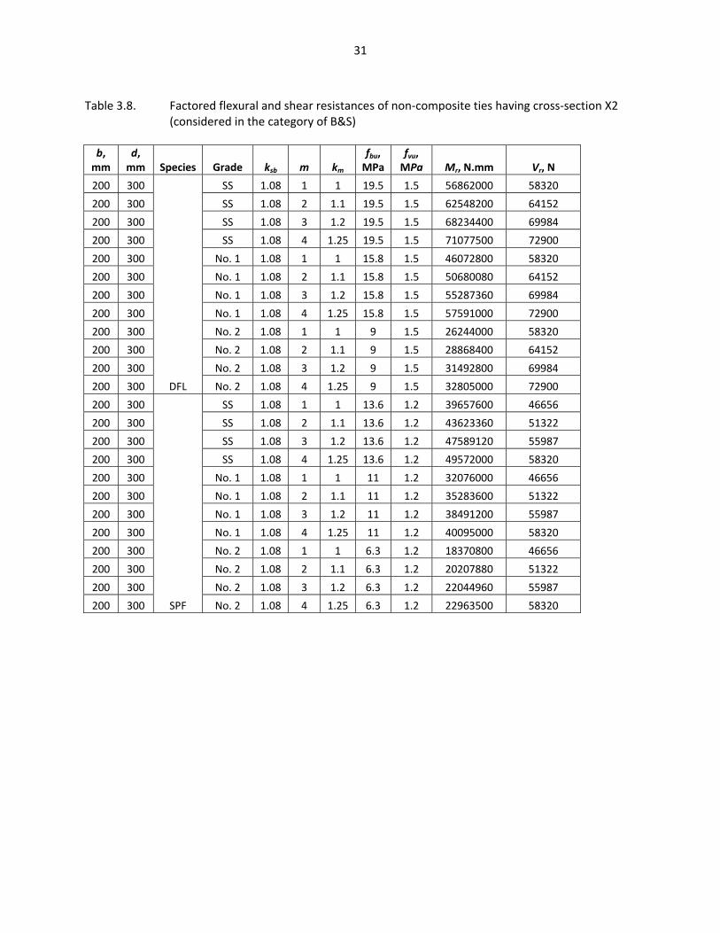
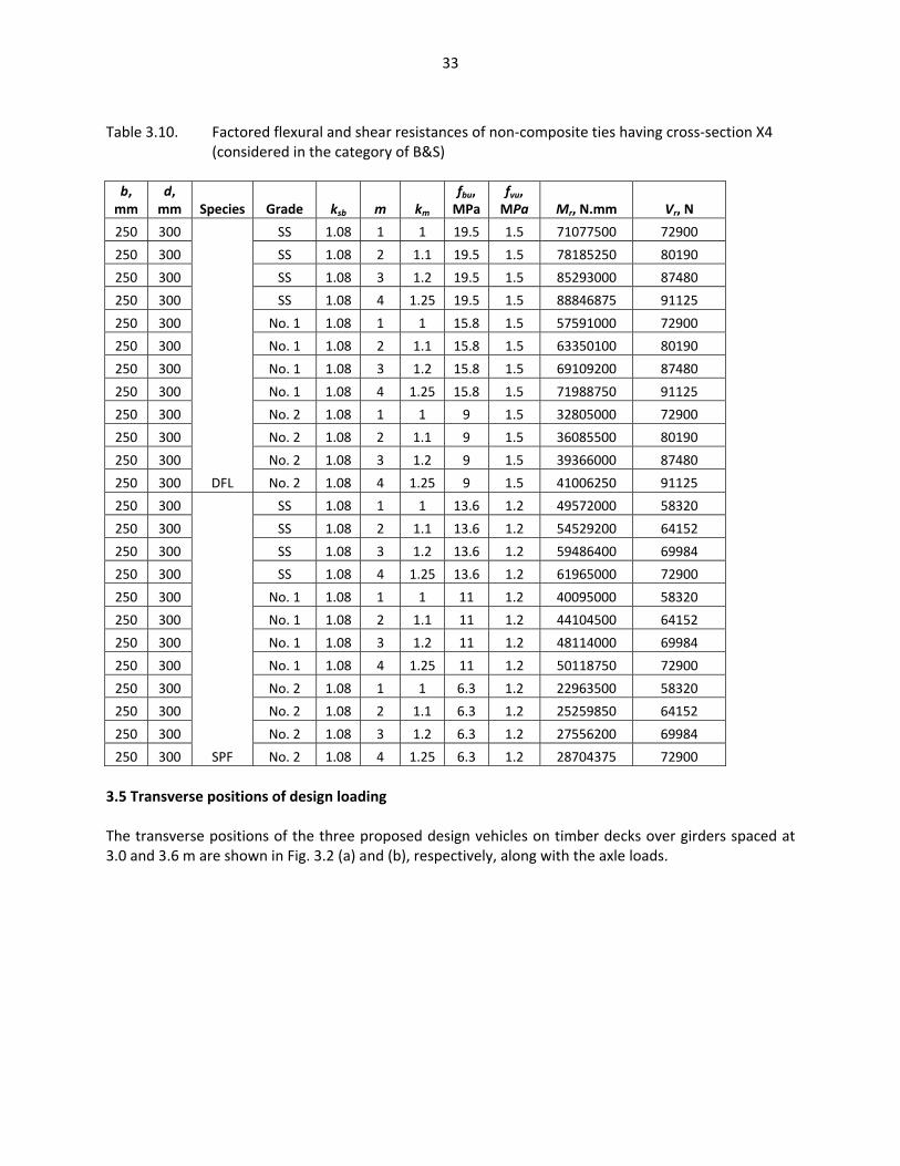
3.4 Calculation of factored resistance The factored flexural and shear resistances of the ties are calculated from Equations (3.1) and (3.2), respectively. As can be seen in these equations, both the flexural and shear resistances of the ties depend upon the load sharing factor, km, which depends upon the number of ties deflecting nearly equally, and which can be found only after analyzing a deck for its load distribution characteristics. The factored flexural and shear resistances of all ties considered in this study were calculated for the values of km ranging between 1 and 4; the values of these factored resistances, i.e. Mr and Vr, are listed in Table 3.7, 3.8, 3.9 and 3.10 for cross-sections X1, X2, X3 and X4, respectively for non-composite ties. Table 3.7. Factored flexural and shear resistances of non-composite ties having cross-section X1 (considered in the category of B&S)

b, mm

d, mm Species Grade ksb m km

fbu, MPa

fvu, MPa Mr, N.mm Vr, N

200 250

DFL

SS 1.17 1 1 19.5 1.5 42778125 52650

200 250 SS 1.17 2 1.1 19.5 1.5 47055938 57915

200 250 SS 1.17 3 1.2 19.5 1.5 51333750 63180

200 250 SS 1.17 4 1.25 19.5 1.5 53472656 65813

200 250 No. 1 1.17 1 1 15.8 1.5 34661250 52650

200 250 No. 1 1.17 2 1.1 15.8 1.5 38127375 57915

200 250 No. 1 1.17 3 1.2 15.8 1.5 41593500 63180

200 250 No. 1 1.17 4 1.25 15.8 1.5 43326563 65813

200 250 No. 2 1.17 1 1 9 1.5 19743750 52650

200 250 No. 2 1.17 2 1.1 9 1.5 21718125 57915

200 250 No. 2 1.17 3 1.2 9 1.5 23692500 63180

200 250 No. 2 1.17 4 1.25 9 1.5 24679688 65813

200 250

SPF

SS 1.17 1 1 13.6 1.2 29835000 42120

200 250 SS 1.17 2 1.1 13.6 1.2 32818500 46332

200 250 SS 1.17 3 1.2 13.6 1.2 35802000 50544

200 250 SS 1.17 4 1.25 13.6 1.2 37293750 52650

200 250 No. 1 1.17 1 1 11 1.2 24131250 42120

200 250 No. 1 1.17 2 1.1 11 1.2 26544375 46332

200 250 No. 1 1.17 3 1.2 11 1.2 28957500 50544

200 250 No. 1 1.17 4 1.25 11 1.2 30164063 52650

200 250 No. 2 1.17 1 1 6.3 1.2 13820625 42120

200 250 No. 2 1.17 2 1.1 6.3 1.2 15202688 46332

200 250 No. 2 1.17 3 1.2 6.3 1.2 16584750 50544

200 250 No. 2 1.17 4 1.25 6.3 1.2 17275781 52650

31

Table 3.8. Factored flexural and shear resistances of non-composite ties having cross-section X2 (considered in the category of B&S)

b, mm


fbu, MPa


200 300

DFL

SS 1.08 1 1 19.5 1.5 56862000 58320

200 300 SS 1.08 2 1.1 19.5 1.5 62548200 64152

200 300 SS 1.08 3 1.2 19.5 1.5 68234400 69984

200 300 SS 1.08 4 1.25 19.5 1.5 71077500 72900

200 300 No. 1 1.08 1 1 15.8 1.5 46072800 58320

200 300 No. 1 1.08 2 1.1 15.8 1.5 50680080 64152

200 300 No. 1 1.08 3 1.2 15.8 1.5 55287360 69984

200 300 No. 1 1.08 4 1.25 15.8 1.5 57591000 72900

200 300 No. 2 1.08 1 1 9 1.5 26244000 58320

200 300 No. 2 1.08 2 1.1 9 1.5 28868400 64152

200 300 No. 2 1.08 3 1.2 9 1.5 31492800 69984

200 300 No. 2 1.08 4 1.25 9 1.5 32805000 72900

200 300

SPF

SS 1.08 1 1 13.6 1.2 39657600 46656

200 300 SS 1.08 2 1.1 13.6 1.2 43623360 51322

200 300 SS 1.08 3 1.2 13.6 1.2 47589120 55987

200 300 SS 1.08 4 1.25 13.6 1.2 49572000 58320

200 300 No. 1 1.08 1 1 11 1.2 32076000 46656

200 300 No. 1 1.08 2 1.1 11 1.2 35283600 51322

200 300 No. 1 1.08 3 1.2 11 1.2 38491200 55987

200 300 No. 1 1.08 4 1.25 11 1.2 40095000 58320

200 300 No. 2 1.08 1 1 6.3 1.2 18370800 46656

200 300 No. 2 1.08 2 1.1 6.3 1.2 20207880 51322

200 300 No. 2 1.08 3 1.2 6.3 1.2 22044960 55987

200 300 No. 2 1.08 4 1.25 6.3 1.2 22963500 58320

32


b, mm


fbu, MPa


250 300

DFL

SS 1.08 1 1 19.5 1.5 71077500 72900

250 300 SS 1.08 2 1.1 19.5 1.5 78185250 80190

250 300 SS 1.08 3 1.2 19.5 1.5 85293000 87480

250 300 SS 1.08 4 1.25 19.5 1.5 88846875 91125

250 300 No. 1 1.08 1 1 15.8 1.5 57591000 72900

250 300 No. 1 1.08 2 1.1 15.8 1.5 63350100 80190

250 300 No. 1 1.08 3 1.2 15.8 1.5 69109200 87480

250 300 No. 1 1.08 4 1.25 15.8 1.5 71988750 91125

250 300 No. 2 1.08 1 1 9 1.5 32805000 72900

250 300 No. 2 1.08 2 1.1 9 1.5 36085500 80190

250 300 No. 2 1.08 3 1.2 9 1.5 39366000 87480

250 300 No. 2 1.08 4 1.25 9 1.5 41006250 91125

250 300

SPF

SS 1.08 1 1 13.6 1.2 49572000 58320

250 300 SS 1.08 2 1.1 13.6 1.2 54529200 64152

250 300 SS 1.08 3 1.2 13.6 1.2 59486400 69984

250 300 SS 1.08 4 1.25 13.6 1.2 61965000 72900

250 300 No. 1 1.08 1 1 11 1.2 40095000 58320

250 300 No. 1 1.08 2 1.1 11 1.2 44104500 64152

250 300 No. 1 1.08 3 1.2 11 1.2 48114000 69984

250 300 No. 1 1.08 4 1.25 11 1.2 50118750 72900

250 300 No. 2 1.08 1 1 6.3 1.2 22963500 58320

250 300 No. 2 1.08 2 1.1 6.3 1.2 25259850 64152

250 300 No. 2 1.08 3 1.2 6.3 1.2 27556200 69984

250 300 No. 2 1.08 4 1.25 6.3 1.2 28704375 72900

33


b, mm


fbu, MPa


250 300

DFL

SS 1.08 1 1 19.5 1.5 71077500 72900

250 300 SS 1.08 2 1.1 19.5 1.5 78185250 80190

250 300 SS 1.08 3 1.2 19.5 1.5 85293000 87480

250 300 SS 1.08 4 1.25 19.5 1.5 88846875 91125

250 300 No. 1 1.08 1 1 15.8 1.5 57591000 72900

250 300 No. 1 1.08 2 1.1 15.8 1.5 63350100 80190

250 300 No. 1 1.08 3 1.2 15.8 1.5 69109200 87480

250 300 No. 1 1.08 4 1.25 15.8 1.5 71988750 91125

250 300 No. 2 1.08 1 1 9 1.5 32805000 72900

250 300 No. 2 1.08 2 1.1 9 1.5 36085500 80190

250 300 No. 2 1.08 3 1.2 9 1.5 39366000 87480

250 300 No. 2 1.08 4 1.25 9 1.5 41006250 91125

250 300

SPF

SS 1.08 1 1 13.6 1.2 49572000 58320

250 300 SS 1.08 2 1.1 13.6 1.2 54529200 64152

250 300 SS 1.08 3 1.2 13.6 1.2 59486400 69984

250 300 SS 1.08 4 1.25 13.6 1.2 61965000 72900

250 300 No. 1 1.08 1 1 11 1.2 40095000 58320

250 300 No. 1 1.08 2 1.1 11 1.2 44104500 64152

250 300 No. 1 1.08 3 1.2 11 1.2 48114000 69984

250 300 No. 1 1.08 4 1.25 11 1.2 50118750 72900

250 300 No. 2 1.08 1 1 6.3 1.2 22963500 58320

250 300 No. 2 1.08 2 1.1 6.3 1.2 25259850 64152

250 300 No. 2 1.08 3 1.2 6.3 1.2 27556200 69984

250 300 No. 2 1.08 4 1.25 6.3 1.2 28704375 72900 3.5 Transverse positions of design loading The transverse positions of the three proposed design vehicles on timber decks over girders spaced at 3.0 and 3.6 m are shown in Fig. 3.2 (a) and (b), respectively, along with the axle loads.

34

Figure 3.2. Transverse position of design vehicles on timber deck: (a) on girder spaced at 3.0 m, (b) on girders spaced at 3.6 m (Note: Maximum wheel loads in Heavy and Light Off- highway Trucks are obtained on 60:40 basis, and those for BCL-525 Design loading on 50:50 basis

0.60 m 2.50 m 0.50 m Heavy Off-highway Truck (factored maximum wheel load = 346 kN)

Light Off-highway Truck (factored maximum wheel load = 199 kN) BCL-625 Loading (factored maximum wheel load = 117 kN)

0.60 m 1.90 m 1.15 m

0.60 m 1.80 m 1.25 m

0.65 m 3.0 m 0.65 m

(a)

0.60 m 2.50 m 1.10 m

0.60 m 1.90 m 1.75 m

0.60 m 1.80 m 1.80 m

0.65 m 3.6 m 0.65 m

(b)

Heavy Off-highway Truck (factored maximum wheel load = 346 kN) Light Off-highway Truck (factored maximum wheel load = 199 kN) BCL-525 Design Loading (factored maximum wheel load = 117 kN)

35

4. Design checks

4.1 Introduction

It is well known that when a series of parallel beams having the same span are subjected to a moving load, the external beam attracts the highest load as it can share load with beams on only one side of it. The internal beams, which have beams on both their sides, can share load with adjacent beams on both sides, because of which the maximum load effects that they receive are smaller than the maximum load effects experienced by external ties. The phenomenon of the external ties experiencing much higher load effects than internal ties can be observed in Figs. 1.14 (a) and (b), in which the external tie is subjected to the same wheel load as one of the internal ties, but receives significantly larger bending moments than the directly loaded internal tie. The problem of the external tie being the most critical tie can be handled in one of the following three ways.

a. Design the external tie for the maximum load effects that it receives and provide the same cross-section for the internal ties; clearly such an arrangement will lead to wasteful design if the span of the structure is long and the method of construction is monolithic.

b. Provide a larger cross-section for the external ties than the cross-section for the internal ties; such an arrangement will require separate analysis of each deck, as the heavier external tie will attract even larger load effects because of their higher flexural rigidity. Further, such an arrangement may not be desirable if the pre-assembled modules are used to make the deck.

c. Provide two side-by-side ties as an individual external ‘tie unit’; this arrangement is expected to provide the most cost-effective solution.

Since there cannot be a clear preference for any of the three arrangements presented above, it was agreed with the MFR personnel that the design check exercise would be conducted for arrangements (a) and (c).

4.2 BCL-625 design loading

It was first required to determine which of Axle No. 4 (with a load of 175 kN) and group of axle Nos. 2 and 3 (with a total weight of 280 kN) of the BCL-625 loading governs designs of the timber decks; to carry out this exercise timber decks on girders at a spacing of 3.0 m and with regularly spaced ties made select structural DFL, i.e. the strongest timber, were checked under both the single 175 kN axle and the two 140 kN axles of the original BCL-625 Truck (Fig. 1.1). For these and all subsequent design checks:

a. the maximum tie moment due to factored ULS loads was compared with the factored moment of resistance of the tie;

b. the maximum deflection of the tie under SLS loads was compared with maximum permissible deflection; and

c. the maximum tie shear due to factored ULS loads was compared with the factored shear resistance of the tie.

For this set of deign checks, the live load factor was taken as 1.7, as specified in S6, and no composite action was assumed between the planking and the tie. The results of this first set of design checks, in which the design is governed by the end ties, are summarized in Table 4.1. It is noted that in this and

36

subsequent similar tables, a cell representing a design criterion contains both the demand (e.g. factored moment) on the tie and its capacity (e.g. the factored moment of resistance), separated by a slash. The cell is coloured green if the design criterion is satisfied, and red if it is not.

Table 4.1. Design checks for end ties for original BCL-625 loading for timber decks made with select structural DFL on girders at a spacing of 3.0 m, assuming no composite action between ties and planks, and with a live load factor = 1.7

Cross-section (dimensions in

mm)

No. of planks

Single/dual axle

Moment, kN.mfactored mt./factored

resistance (ULS)

Deflection, mmpermissible/SLS

deflection

Shear, kNfactored shear/factored

resistance (ULS)

X1

1

Single 75/43 7.9/7.5 94/53

1

Dual 66/43 7.4/7.5 75/53

2

Single 59/43 5.7/7.5 70/53

2

Dual 57/43 6.3/7.5 62/53

X2

1

Single 82/57 5.1/7.5 102/58

1

Dual 69/57 4.5/7.5 79/58

2

Single 64/57 3.7/7.5 78/58

2

Dual 60/57 3.9/7.5 66/58

X3

1

Single 84/71 4.2/7.5 106/73

1

Dual 70/71 3.7/7.5 81/73

2

Single 67/71 3.1/7.5 81/73

2

Dual 62/71 3.2/7.5 68/73

X4 1

Single 75/71 3.6/7.5 94/73

1

Dual 61/71 3.1/7.5 71/73

2

Single 59/71 2.6/7.5 70/73

2

Dual 53/71 2.6/7.5 57/73

It can be seen in Table 4.1 that all except four decks made with ties of the strongest timber and supported on girders at a spacing of 3.0 m and subjected to the lightest of the three design loads, fail to meet the shear design criterion when no composite action is assumed between the planking and the ties. When the composite action is considered for the same set of decks and loading as considered for Table 4.1, the results of the design checks are as listed in Table 4.2, in which all except two decks still fail to meet all the design criteria. Similar to Table 4.1, Table 4.2 also shows that the design of all ties is still governed by shear, which is little affected by the composite action. It is noted the flexural resistances of

37

the composite ties by increasing the flexural resistance of the non-composite ties by the percentage increases in column No. 6 of Tables 3.3 through 3.6. Table 4.2. Design checks for end ties for original BCL-625 loading for timber decks made with select structural DFL on girders at a spacing of 3.0 m, assuming full composite action between ties and planks, and with a live load factor = 1.7

Cross-section No. of planks

Single/dual axle

Moment, kN.m factored mt./factored

resistance (ULS)

Deflection, mm permissible/SLS

deflection

Shear, kN factored shear/factored

resistance (ULS) X1

1

Single 76/46 7.9/7.5 94/53

1

Dual 66/46 7.4/7.5 75/53

2

Single 59/48 5.7/7.5 70/53

2

Dual 57/48 6.3/7.5 62/53

X2

1

Single 82/59 5.1/7.5 102/58

1

Dual 69/59 4.5/7.5 79/58

2

Single 64/61 3.7/7.5 78/58

2

Dual 60/61 3.9/7.5 66/58

X3

1

Single 84/73 4.2/7.5 106/73

1

Dual 70/73 3.7/7.5 81/73

2

Single 67/75 3.1/7.5 81/73

2

Dual 62/75 3.2/7.5 68/73

X4

1

Single 75/73 3.6/7.5 94/73

1

Dual 61/73 3.1/7.5 71/73

2

Single 59/75 2.6/7.5 70/73

2

Dual 53/75 2.6/7.5 57/73

It can also be seen in Tables 4.1 and 4.2 that in all decks, axle No. 4 of the original BCL-625 loading induces higher load effects than the two-axle group of axles Nos. 2 and 3. For reasons expounded in the following, it is recommended that axle No. 4 of the original BCL-625 not be used to the design of timber decks under consideration, nor for the design of any other deck systems (concrete deck slabs and steel plate decks) in British Columbia. The CL-625 Truck of S6 is based on survey data obtained for vehicle and axle weights in Ontario. While the calibration report for S6 (CSA, 2006-2) does not directly list the Ontario data for axle or wheel loads, such data can be calculated from information given in this report. Assuming that wheel loads on axles

38

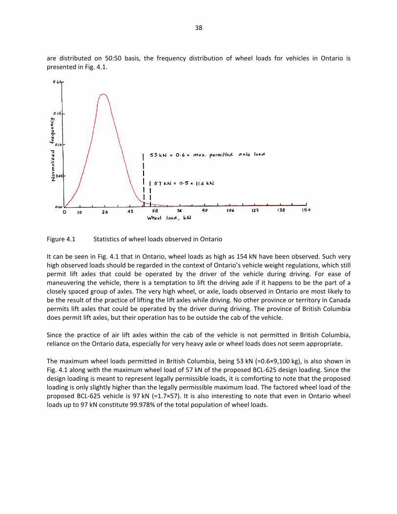
are distributed on 50:50 basis, the frequency distribution of wheel loads for vehicles in Ontario is presented in Fig. 4.1.

Figure 4.1 Statistics of wheel loads observed in Ontario It can be seen in Fig. 4.1 that in Ontario, wheel loads as high as 154 kN have been observed. Such very high observed loads should be regarded in the context of Ontario’s vehicle weight regulations, which still permit lift axles that could be operated by the driver of the vehicle during driving. For ease of maneuvering the vehicle, there is a temptation to lift the driving axle if it happens to be the part of a closely spaced group of axles. The very high wheel, or axle, loads observed in Ontario are most likely to be the result of the practice of lifting the lift axles while driving. No other province or territory in Canada permits lift axles that could be operated by the driver during driving. The province of British Columbia does permit lift axles, but their operation has to be outside the cab of the vehicle. Since the practice of air lift axles within the cab of the vehicle is not permitted in British Columbia, reliance on the Ontario data, especially for very heavy axle or wheel loads does not seem appropriate. The maximum wheel loads permitted in British Columbia, being 53 kN (=0.6×9,100 kg), is also shown in Fig. 4.1 along with the maximum wheel load of 57 kN of the proposed BCL-625 design loading. Since the design loading is meant to represent legally permissible loads, it is comforting to note that the proposed loading is only slightly higher than the legally permissible maximum load. The factored wheel load of the proposed BCL-625 vehicle is 97 kN (=1.7×57). It is also interesting to note that even in Ontario wheel loads up to 97 kN constitute 99.978% of the total population of wheel loads.

39

Table 4.3. Design checks for external ties original design and with following parameters: (a) S = 3.0 m, (b) full composite action, αL = 1.7

Cross-section Species Grade No. of planks

Design loadingBCL-625 Light Off-

highway

X4

DFL SS 2 V SS 1 M, V 1 2 M, V 1 1 M M, V 2 2 M M, V 2 1 M M, w, V

SPF SS 2 M, w, V SS 1 M, w, V 1 2 M, w, V 1 1 M M, w, V 2 2 M M, w, V 2 1 M M, w, V

X3

DFL SS 2 M, V SS 1 V M, w, V 1 2 M, V M, V 1 1 M, V M, w, V 2 2 M M, w, V 2 1 M M, w, V

SPF SS 2 M, w, V SS 1 V M, w, V 1 2 M, V M, w, V 1 1 M, w, V M, w, V 2 2 M, w, V M, w, V 2 1 M, w, V M, w, V

X2

DFL SS 2 V M, w, V SS 1 M, V M, w, V 1 2 M, V M, w, V 1 1 M, V M, w, V 2 2 M, V M, w, V 2 1 M, w, V M, w, V

SPF SS 2 M, V M, w, V SS 1 M. V M, w, V 1 2 M, V M, w, V 1 1 M, w, V M, w, V 2 2 M, w, V M, w, V 2 1 M, w, V M, w, V

X1

DFL SS 2 M, V M, w, V SS 1 M, V M, w, V 1 2 M, V M, w, V 1 1 M, V M, w, V 2 2 M, w M, w, V 2 1 M, w, V M, w, V

SPF SS 2 M, w, V M, w, V SS 1 M, w, V M, w, V 1 2 M, w, V M, w, V 1 1 M, w, V M, w, V 2 2 M, w, V M, w, V 2 1 M, w, V M, w, V

M, w, V M, w, V

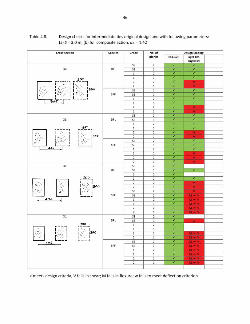
meets design criteria; V fails in shear; M fails in flexure; w fails to meet deflection criterion

40

4.3 Design checks with proposed loadings

All design checks, presented in this sub-section, were performed under the three proposed design loadings, being Heavy Off-highway Design loading (Fig. 1.15), Light Off-highway Design loading (Fig. 1.18) and BCL-625 loading (Fig. 1.19). In all cases, full composite action was assumed between the planks and the ties. As noted earlier, the flexural resistances of all cross-sections were calculated by assuming that these cross-sections can be considered in the category of beam & stringers (B&S), whereas in accordance with the NLGA grading rules, cross-sections X1, X3 and X4 should be regarded in the category of post & timber (P&T). 4.3.1 Design checks for external ties with original design The design checks for all timber decks on stringers at a spacing of 3.0 m, and with a clear width of 4.3 m, are presented in Table 4.3 for a live load factor of 1.7 for the proposed BCL-625 and Light Off-highway Design loadings, it being noted that the 4.3 m width of the deck cannot realistically accommodate the wide Heavy Off-highway Design truck. It can be seen in Table 4.3 that the external ties of all timber decks fail to meet the design criteria under the proposed Light Off-highway Design loading. The failure occurs almost in the three categories of checks: for moments, deflections and shears. It follows that these ties will also fail to meet the S6 design criteria under the Heavy Off-highway Design truck, even if this truck could be accommodated on the narrow deck. Only a few of the external ties manage to meet the S6 design criteria under the proposed BCL-625 Design loading. As noted earlier, the design checks in Table 4.3 were performed for a live load factor of 1.7. When Ontario Ministry of Natural Resources found that many of its timber decks failed to meet the design criteria of S6-06, it decided to lower the reliability index for timber decks from 3.50 to 2.75, and to reduce the live load factor, αL, from 1.70 to 1.42 (ref missing). The evaluation section of S6-06 in its Clause 14.13.3.1 also specifies αL = 1.42 for reliability index of 2.75 corresponding to normal traffic. The reduced value of αL and the axle load of 140 kN give the factored load of 199 kN. In Fig. 1.19, the BCL-625 design loading for timber decks, based on survey data is recommended to be a 2-axle group with an inter-axle spacing of 1.37 m, with each axle carrying a load of 117 kN. Fortuitously, when a load factor of 1.7 is used with axle weight of 117 kN, the factored is 199 kN, the same factored load which corresponds to αL = 1.42 and the axle weight of 140 kN. It should, however, be noted that the inter-axle spacing of the loading proposed in Fig. 1.19 is 1.37 m, as compared to the spacing of 1.2 m in the BCL-625 loading.

The same design checks which were performed for Table 4.3 for a live load factor of 1.7 were repeated with a live load factor of 1.42; the results of this latter set of checks are summarized in Table 4.4, in which it can be seen that while the situation improves under the proposed BCL-625 Design loading, all decks except two fail to meet the design criteria of S6.

41

Table 4.4. Design checks for external ties original design and with following parameters: (a) S = 3.0 m, (b) full composite action, αL = 1.42



highway

X4

DFL SS 2 SS 1 M, w 1 2 1 1 M 2 2 M 2 1 M M, V

SPF SS 2 M, V SS 1 M, w, V 1 2 M, V 1 1 M, V 2 2 M M, w 2 1 M M, w, V

X3

DFL SS 2 V SS 1 M, V 1 2 M, V 1 1 M, V 2 2 M M, w, V 2 1 M M, w, V

SPF SS 2 M, w, V SS 1 M, w, V 1 2 M, w, V 1 1 M M, w, V 2 2 M M, w, V 2 1 M M, w, V

X2

DFL SS 2 M, w, V SS 1 V M, w, V 1 2 V M, w, V 1 1 M, V M, w, V 2 2 M M, w, V 2 1 M M, w, V

SPF SS 2 M, w, V SS 1 M, w, V 1 2 M, w, V 1 1 M M, w, V 2 2 M, w M, w, V 2 1 M, w, V M, w, V

X1

DFL SS 2 M, w, V SS 1 M, V M, w, V 1 2 M, V M, w, V 1 1 M, V M, w, V 2 2 M M, w, V 2 1 M M, w, V

SPF SS 2 M, w M, w, V SS 1 M, w, V M, w, V 1 2 M, w M, w, V 1 1 M, w, V M, w, V 2 2 M, w, V M, w, V 2 1 M, w, V M, w, V


42

The same design checks which were performed for external ties in decks on girders spaced at 3.0 m (Tables 4.3 and 4.4) were repeated for external ties in decks on girders at a spacing of 3.6 m. The result corresponding to the live load factors of 1.7 and 1.42 are summarized in Tables 4.5 and 4.6, respectively. As expected, when the live load factor is 1.7, external ties in nearly all decks fail to meet the S6 design criteria for all three loadings. The situation does not improve considerably when the live load factor is reduced to 1.42. Table 4.5. Design checks for external ties original design and with following parameters: (a) S = 3.6 m, (b) full composite action, αL = 1.7



highway Heavy

Off-highway

X4

DFL SS 2 M, w, V M, w, VSS 1 M, w, V M, w, V1 2 M, w, V M, w, V1 1 M, w, V M, w, V2 2 M, w M, w, V M, w, V2 1 M, w, V M, w, V M, w, V

SPF SS 2 w, V M, w, V M, w, VSS 1 M, w, V M, w, V M, w, V1 2 M, w, V M, w, V M, w, V1 1 M, w, V M, w, V M, w, V2 2 M, V M, w, V M, w, V2 1 M, w, V M, w, V M, w, V

X3

DFL SS 2 M, w, V M, w, VSS 1 w M, w, V M, w, V1 2 M, w, V M, w, V1 1 M, w M, w, V M, w, V2 2 M, w M, w, V M, w, V2 1 M, w M, w, V M, w, V

SPF SS 2 M, w M, w, V M, w, VSS 1 M, w M, w, V M, w, V1 2 M, w M, w, V M, w, V1 1 M, w, V M, w, V M, w, V2 2 M, w M, w, V M, w, V2 1 M, w, V M, w, V M, w, V

X2

DFL SS 2 w M, w, V M, w, VSS 1 M, w, V M, w, V M, w, V1 2 M, w M, w, V M, w, V1 1 M, w, V M, w, V M, w, V2 2 M, w, V M, w, V M, w, V2 1 M, w, V M, w, V M, w, V

SPF SS 2 M, w, V M, w, V M, w, VSS 1 M, w, V M, w, V M, w, V1 2 M, w, V M, w, V M, w, V1 1 M, w, V M, w, V M, w, V2 2 M, w, V M, w, V M, w, V2 1 M, w, V M, w, V M, w, V1 2 M, w, V M, w, V M, w, V1 1 M, w, V M, w, V M, w, V2 2 M, w, V M, w, V M, w, V2 1 M, w, V M, w, V M, w, V


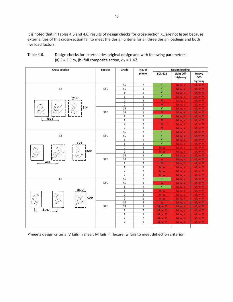
43

It is noted that in Tables 4.5 and 4.6, results of design checks for cross-section X1 are not listed because external ties of this cross-section fail to meet the design criteria for all three design loadings and both live load factors. Table 4.6. Design checks for external ties original design and with following parameters: (a) S = 3.6 m, (b) full composite action, αL = 1.42



highway Heavy

Off-highway

X4

DFL SS 2 M, w, V M, w, VSS 1 M, w, V M, w, V1 2 M, w, V M, w, V1 1 M, w, V M, w, V2 2 M M, w, V M, w, V2 1 M M, w, V M, w, V

SPF SS 2 M, w, V M, w, VSS 1 V M, w, V M, w, V1 2 M, w, V M, w, V1 1 M M, w, V M, w, V2 2 M M, w, V M, w, V2 1 M M, w, V M, w, V

X3

DFL SS 2 M, w, V M, w, VSS 1 M, w, V M, w, V1 2 M, w, V M, w, V1 1 M, w, V M, w, V2 2 M, w M, w, V M, w, V2 1 M, w M, w, V M, w, V

SPF SS 2 M, w, V M, w, VSS 1 w M, w, V M, w, V1 2 M M, w, V M, w, V1 1 M, w M, w, V M, w, V2 2 M, w M, w, V M, w, V2 1 M, w M, w, V M, w, V

X2

DFL SS 2 M, w, V M, w, VSS 1 w M, w, V M, w, V1 2 M, w, V M, w, V1 1 M, w M, w, V M, w, V2 2 M, w M, w, V M, w, V2 1 M, w M, w, V M, w, V

SPF SS 2 w M, w, V M, w, VSS 1 M, w, V M, w, V M, w, V1 2 M, w, V M, w, V M, w, V1 1 M, w, V M, w, V M, w, V2 2 M, w, V M, w, V M, w, V2 1 M, w, V M, w, V M, w, V


44

4.3.2 Design checks for internal ties with original design The design checks for internal ties in decks with the original design and supported on girders at spacing of 3.0 m are summarized in Tables 4.7 and 4.8 for live load factors of 1.7 and 1.42, respectively. It can be seen in Table 4.7 that with live load factor 1.7, most of internal ties with cross-sections X4 and X3 meet the S6 design requirements under the proposed BCL-625 loading. However, only a few decks meet the S6 design requirement under the proposed Light Off-highway Design loading. By reducing the live load factor from 1.7 to 1.42, internal ties of all decks meet the S6 design requirements under the proposed BCL-625 loading. Internal ties of nearly half the decks fail to meet the design requirements under the Light Off-highway loading. The design checks for internal ties in decks with the original design and supported on girders at a spacing of 3.6 m are summarized in Tables 4.9 and 4.10 for live load factor = 1.7 and 1.42. For the live load factor of 1.7, all internal ties fail to meet the design criteria under the proposed Heavy and Light Off-highway Design loadings. Under the proposed BCL-625 loading, many internal ties with cross-sections X4 and X3 meet the design requirements. When the live load factor is reduced to 1.42, only internal ties with cross-section X4 and made with DFL select structural grade and Grade No. 1 meet the design requirements under the proposed Light Off-highway Design loading. However, internal ties of all decks fail to meet the design requirement under Heavy Off-highway Design loading even when the live load factor is reduced to 1.42

45

Table 4.7. Design checks for intermediate ties original design and with following parameters: (a) S = 3.0 m, (b) full composite action, αL = 1.7



highway

X4

DFL SS 2 SS 1 1 2 1 1 2 2 M 2 1 M

SPF SS 2 V SS 1 V 1 2 M, V 1 1 M, V 2 2 M M, V 2 1 M M, V

X3

DFL SS 2 SS 1 1 2 1 1 2 2 M2 1 M

SPF SS 2 V SS 1 M, V 1 2 M, V 1 1 M, V 2 2 M M, V 2 1 M M, V

X2

DFL SS 2 SS 1 M, V 1 2 M, V 1 1 M, V 2 2 M M, V 2 1 M M, V

SPF SS 2 M, V SS 1 M, V 1 2 M, V 1 1 M, V 2 2 M, w M, w, V 2 1 M, w M, w, V

X1

DFL SS 2 SS 1 M, V 1 2 1 1 2 2 M, w M, w, V 2 1 M, w M, w, V

SPF SS 2 w, V M, w, V SS 1 w M, w, V 1 2 M, w, V M, w, V 1 1 M, w M, w, V 2 2 M, w, V M, w, V 2 1 M, w M, w, V


46




highway

X4

DFL SS 2 SS 1 1 2 1 1 2 2 M 2 1 M

SPF SS 2 SS 1 1 2 1 1 2 2 M 2 1 M

X3

DFL SS 2 SS 1 1 2 1 1 2 2 M 2 1 M

SPF SS 2 SS 1 1 2 1 1 M 2 2 M 2 1 M

X2

DFL SS 2 SS 1 1 2 1 1 2 2 M 2 1 M

SPF SS 2 V SS 1 M, w, V 1 2 M, w, V 1 1 M, w, V 2 2 M, w, V 2 1 M, w, V

X1

DFL SS 2 SS 1 w 1 2 1 1 2 2 M, w, V 2 1 M, w, V

SPF SS 2 M, w, V SS 1 M, w, V 1 2 M, w, V 1 1 M, w, V 2 2 M, w, V 2 1 M, w, V


47




highway Heavy

Off-highway

X4

DFL SS 2 w M, w, VSS 1 w M, w, V1 2 w M, w, V1 1 M, w M, w, V2 2 M, w M, w, V2 1 M, w M, w, V

SPF SS 2 M, w, V M, w, VSS 1 M, w, V M, w, V1 2 M, w, V M, w, V1 1 M, w, V M, w, V2 2 M, w M, w, V M, w, V2 1 M, w M, w, V M, w, V

X3

DFL SS 2 w, V M, w, VSS 1 w, V M, w, V1 2 M, w, V M, w, V1 1 M, w, V M, w, V2 2 M M, w, V M, w, V2 1 M, w M, w, V M, w, V


X2

DFL SS 2 M, w, V M, w, VSS 1 w M, w, V M, w, V1 2 M, w, V M, w, V1 1 w M, w, V M, w, V2 2 M, w M, w, V M, w, V2 1 M, w M, w, V M, w, V

SPF SS 2 w M, w, V M, w, VSS 1 w M, w, V M, w, V1 2 M, w M, w, V M, w, V1 1 M, w M, w, V M, w, V2 2 M, w M, w, V M, w, V2 1 M, w M, w, V M, w, V


48




highway Heavy

Off-highway

X4

DFL SS 2 w, VSS 1 w, V1 2 M, w, V1 1 M, w, V2 2 w M, w, V2 1 w M, w, V

SPF SS 2 w M, w, VSS 1 w M, w, V1 2 M, w M, w, V1 1 M, w M, w, V2 2 M M, w M, w, V2 1 M, w M, w M, w, V

X3

DFL SS 2 w w, VSS 1 w w, V1 2 w M, w, V1 1 w M, w, V2 2 M, w M, w, V2 1 M, w M, w, V


X2

DFL SS 2 M, w, V M, w, VSS 1 M, w, V M, w, V1 2 M, w, V M, w, V1 1 M, w, V M, w, V2 2 M M, w, V M, w, V2 1 M, w M, w, V M, w, V

SPF SS 2 w M, w, V M, w, VSS 1 w M, w, V M, w, V1 2 w M, w, V M, w, V1 1 w M, w, V M, w, V2 2 M, w M, w, V M, w, V2 1 M, w M, w, V M, w, V

X1

DFL SS 2 M, w, V M, w, VSS 1 M, w, V M, w, V1 2 M, w M, w, V M, w, V1 1 M, w M, w, V M, w, V2 2 M, w M, w, V M, w, V2 1 M, w M, w, V M, w, V

SPF SS 2 M, w M, w, V M, w, VSS 1 M, w M, w, V M, w, V1 2 M, w M, w, V M, w, V1 1 M, w M, w, V M, w, V2 2 M, w M, w, V M, w, V2 1 M, w M, w, V M, w, V


49

4.3.3 Design checks for external ties with revised design As noted in Section 4.1 (c), one of the possible ways to improve the design of external ties is to provide two side-by-side ties as an individual tie unit. Decks with ties having X4 cross-section and spanning over girders at spacing of 3.6 m were checked with the revised design for the external ties. The results of this design-check exercise are listed Tables 4.11 and`4.12 for live load factor = 1.7 and 1.42, respectively. Table 4.11. Design checks for external ties of revised design and with following parameters: (a) S = 3.6 m, (b) full composite action, αL = 1.7



highway Heavy

Off-highway

X4

DFL SS 2 w M, w, VSS 1 w M, w, V1 2 M, w M, w, V1 1 M, w M, w, V2 2 M M, w M, w, V2 1 M M, w M, w, V

SPF SS 2 M, w M, w, VSS 1 M, w, V M, w, V1 2 M, w, V M, w, V1 1 M, w, V M, w, V2 2 M M, w M, w, V2 1 M M, w, V M, w, V

meets design criteria; V fails in shear; M fails in flexure; w fails to meet deflection criterion Table 4.12. Design checks for external ties of revised design and with following parameters: (a) S = 3.6 m, (b) full composite action, αL = 1.42



highway Heavy

Off-highway

X4

DFL SS 2 VSS 1 M, w, V1 2 M, w, V1 1 M, w, V2 2 M, w M, w, V2 1 M, w M, w, V

SPF SS 2 M, w M, w, VSS 1 M, w M, w, V1 2 M, w M, w, V1 1 M, w M, w, V2 2 M M, w M, w, V2 1 M M, w M, w, V

meets design criteria; V fails in shear; M fails in flexure; w fails to meet deflection criterion Live load factor of 1.7. A comparison of Tables 4.5 and 4.11 will readily show that under Heavy and Light Off-highway loadings with a live load factor of 1.7, the revision of the design of external ties did not change the outcome: all analyzed decks failed to meet the design criteria. However, under BCL-625

50

loading with a live factor of 1.7, four decks with revised design, which had failed to meet the design criteria earlier, now meet the design criteria. Live load factor of 1.42. A comparison of Tables 4.6 and 4.12 shows that under Heavy Off-highway loading, the analyzed decks failed to meet the design criteria even after the lowering of the live load factor. However, four decks with revised design under Light Off-highway loading, and four decks with revised design under BCL-625 loading were able to meet the design criteria. 5. Conclusions The conclusions from the design-check exercise for the 48 original deck designs are summarized in Table 5.1 with respect to the three proposed design loadings applied with the live load factors of 1.7 and 1.42. Table 5.1 Outcome of design-check exercise for original designs of the timber decks Design loading

Live load factor

Girder spacing, m

External ties Internal ties

Heavy Off- highway

1.7 3.0 All fail in moment, deflection and shear

All fail in moment, deflection and shear3.6

1.42 3.0 3.6

Light Off- highway

1.7 3.0 All but 1 fail in moment; all but 7 fail in deflection; all fail in shear



All fail, mostly in moment and shear

1.42 3.0 All but 3 fail in moment; all but 9 fail in deflection; all but 2 fail in shear

Slightly more than half fail; most failures in moment and shear



BCL-625 1.7 3.0 All but 8 fail; most failures in moment and shear


3.6 All but 6 fail; most failures in moment and shear


1.42 3.0 More than half fail; most failures in moment and shear

All meet design requirements

3.6 More than half fail; most failures in moment and shear


The revised design, in which two side-by-side ties are used as an external tie unit, improved the situation only marginally.

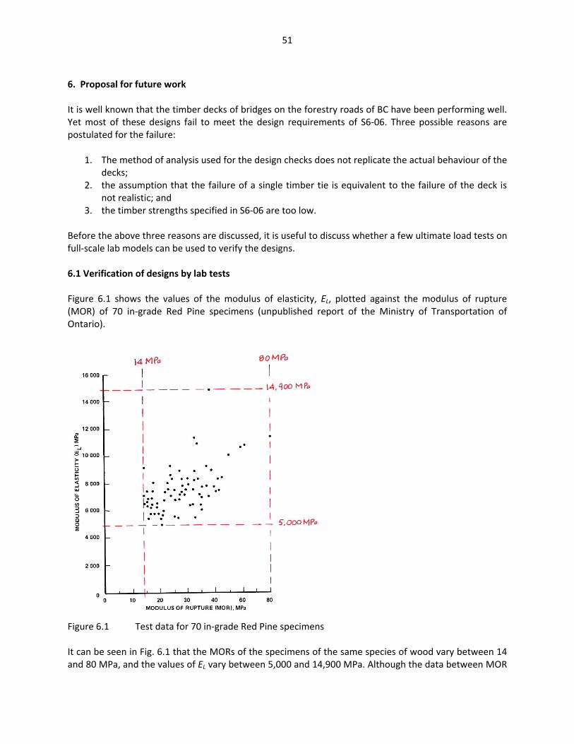
51

6. Proposal for future work It is well known that the timber decks of bridges on the forestry roads of BC have been performing well. Yet most of these designs fail to meet the design requirements of S6-06. Three possible reasons are postulated for the failure:

1. The method of analysis used for the design checks does not replicate the actual behaviour of the decks;

2. the assumption that the failure of a single timber tie is equivalent to the failure of the deck is not realistic; and

3. the timber strengths specified in S6-06 are too low. Before the above three reasons are discussed, it is useful to discuss whether a few ultimate load tests on full-scale lab models can be used to verify the designs. 6.1 Verification of designs by lab tests Figure 6.1 shows the values of the modulus of elasticity, EL, plotted against the modulus of rupture (MOR) of 70 in-grade Red Pine specimens (unpublished report of the Ministry of Transportation of Ontario).

Figure 6.1 Test data for 70 in-grade Red Pine specimens It can be seen in Fig. 6.1 that the MORs of the specimens of the same species of wood vary between 14 and 80 MPa, and the values of EL vary between 5,000 and 14,900 MPa. Although the data between MOR

52

and EL are strongly co-related, the co-relation is not perfect, so that a stringer with a high value of EL, attracting higher loads, does not necessarily have a high value of MOR. The effect of the random variation of EL on load distribution was investigated by Bakht (1983) through Monte Carlo simulations of 60 sawn timber decks. It was found that in each deck with randomly distributed values of EL, the pattern of transverse distribution of moments in the stringers was highly uneven. As shown in Fig. 6.2, the upper- and lower-bound values of stringer moments, and their mean values, followed patterns that could be predicted statistically. An exact analysis of a timber deck is impossible to perform unless the value of EL for each tie is known beforehand.

Figure 6.2 Effect of EL on transverse load distribution

Dis

trib

utio

n fa

ctor

s fo

r de

flect

ions

D

istr

ibut

ion

fact

ors

for

mom

ents

in s

trin

gers

53

In contrast with the distribution of stringer moments, the distribution of stringer deflections in all the simulated decks was nearly the same (Fig. 6.2). It may be observed in Fig. 6.2 that the mean values of stringer moments (obtained from analysis results of 60 simulations) are very close to the moments obtained by assuming that EL for all stringers is the 50th percentile, i.e. E50 as specified in S6-06. This observation confirms the usefulness of a method of analysis in predicting the mean values of the stringer (or tie) moments. It is possible that the variations in the values of MOR and EL in DFL and SPF specimens may be larger or smaller than those in the Red Pine specimens. However, it is well established that all species of timber have fairly large variation in the values of their MOR and EL. The above observations lead to two important conclusions.

1. The failure loads of all timber decks with the same design have a large statistical distribution, the properties of which can be established only by testing a large number, say 15, of decks; it is virtually impossible to draw realistic conclusions about the load carrying capacity of timber decks on the basis of only one or two tests.

2. Measured deflections of in-service bridges under known truck loads can be used to verify a method of analysis, which in turn can be used for design calculations, it being noted that the load sharing factor, which was developed specifically for laminated timber decks to account for the variability of the laminate responses, does not seem to work for timber decks with ties (because the number of ties deforming nearly equally is rarely higher than one).

6.2 Verification of method of analysis It is proposed that least one bridge of each of the four designs considered in this study be tested under a slow-moving truck of known axle weights and spacings. During the tests, deflections of stringers mid-way between the girders should be measured with respect to a temporary platform attached to the lower flanges of the two girders. Of special importance will be the deflections of the external stringers under wheel loads directly over these stringers. 6.3 Failure of one component The design provisions of S6-06 imply that the failure of a component should be regarded as the ultimate limit state (ULS) of the deck. This requirement seems overly conservative. It is possible that an alternate load path is created before the failure of a tie in either moment or shear, thus preventing the failure of the deck. A timber tie has to undergo large deformations before failing in either moment or shear. Since such large deformations are likely to be prevented by the planks and adjacent ties, the ‘failure’ of a single tie might be only theoretical. A few lab tests might be useful is establishing whether a single tie can fail without the adjacent ties. Bakht and Jaeger (1985) had started a study on computer simulation of failure in sawn timber bridges, and Jaeger and Bakht (1985 and 1987) had initiated a study on the probabilistic assessment of failure of laminated timber decks. Despite their promise, these studies were not brought to fruition because of lack of time and funding. It is proposed to revive these studies for the MFR timber decks, so that advantage can be taken of the progressive failure of several ties at the ULS.

54

6.4 Conservative values of specified strengths The values of the specified bending and shear strengths of S6-06 were arrived at after studying the results of extensive in-grade testing, and due adjustment by the Technical Subcommittee for such factors as moisture content and load duration. Some adjustments were also made to the specified strengths as a result of a rigorous calibration exercise. It does not appear appropriate to change most of these values without the consent of the Technical Subcommittee and the Calibration Committee of S-6. The specified shear strength for ties in the MFR timber deck, however, could be revised for the reasons discussed below. The commentary to S6-00 states (in Clause C9.11.2) that the specified shear strengths in S6-00 were based on actual distributions of the check lengths of the in-grade specimens that were tested to obtain the shear strength data. However, the specified sear strengths in S6-00 were very low, ranging between 0.6 and 0.9 MPa for beam and stringer grades. Although not stated in the commentary, the specified shear strengths in S6-00 were based on the work of Foschi and Barrett (1976). In S6-06, the specified shear strengths were raised considerably; for beam stringer grades, the specified shear strength now ranges between 1.0 and 1.5 MPa. The commentary to S6-06 does not give a reason for the increase in the specified shear strengths.

Figure 6.3 Effect of support on shear strength of a timber beam The specified shear strengths of both S6-00 and S6-06, are based on the assumption that the timber beam, or stringer is supported near its ends. As illustrated in Fig. 6.3 (a), the checks (or horizontal splits) in a timber beam also occur near it ends. When a beam is supported near its ends, the presence of checks reduces its shear capacity considerably. For the MFR timber decks, the ties are not supported near their ends. As illustrated in Fig. 6.3 (b), the supports for the ties, being the top flanges of the two steel girders, are well away from their ends, so that the presence of checks at the ends is likely to have virtually no effect on the shear strength of the ties.

(a)

(b)

55

It is proposed that the work of Foschi and Barrett (1976) be re-visited to re-calculate the specified shear strength of beams and stringers that are not supported near their ends. It is expected that the outcome of such an exercise will not be in violation of the spirit of the code, and will lead to substantially higher shear strengths. 7. References

• Bakht. B. Statistical analysis of timber bridges. l983. ASCE Journal of the Structural Division. Vol. l09, No. ST8, pp. l76l-l779.

• Bakht, B. and Jaeger, L.G. l985. Computer simulation of failure in timber bridges. Second International Conference on Computing in Civil Engineering, Hangchou, China, June 5 - 9, pp.484-494, Elsevier, Amsterdam.

• Bakht, B., Mufti, A., and Tadros, G. Nov. 10, 2007. Distribution of wheel loads through planks. Report submitted to MFR.

• BC Bridge Design Truck & Lane Load, Supplement to CHBDC S6-06. April, 2007. British Columbia Ministry of Transportation.

• CAN/CSA-S6-06. Canadian Highway Bridge Design Code. CSA. Toronto. • Cheung, M.S., Bakht, B. and Jaeger, L.G. l982. Analysis of Box Girder Bridges by Grillage and

Orthotropic Plate Methods. Canadian Journal of Civil Engineering. Vol. 9, No.4, p.595-601. • Foschi, R.O., and Barrett, J.D. 1976.Longitudinal shear strength of Douglas-fir. Canadian Journal

of Civil Engineering, Vol. 3, No. 2, pp. 198-208. • Jaeger, L.G., and Bakht, B. l984. Probabilistic assessment of the failure of timber laminated

bridges. Unpublished report. • Jaeger, L.G. and Bakht, B. 1989. Bridge Analysis by Micro-computer. McGraw Hill, New York. • Jaeger, L.G. and Bakht, B. l987. Effect of Transverse Deflection Profile on the Failure Load of

Laminated Wood Bridges. Fifth International Conference on Probability in Soil and Structural Mechanics, May 25 - 29, Vancouver.

• MNR, ref. to come • Mufti, A.A., Bakht, B., Jaeger, L.G., and Jalali, J. 2003. SECAN4 User Manual. ISIS Canada,

University of Manitoba. • NLGA. 2003. Standard Grading Rules for Timber. National Lumber Grades Authority, New

Westminster, BC. • OHBDC. 1993. Ontario Highway Bridge Design Code, Ministry of Transportation of Ontario,

Downsview, Ontario. • Penner, M. 2008. Private communication.

56

Appendix 0 Advice from Buckland & Taylor Ltd. re. Design categories of surveyed vehicles Project: 1579 Date: 2007 September 21 Hi Mike, I've quickly reviewed Baidar's questions and have the following responses: 1. On the TimberWest - Honeymoon Bay Division spreadsheet, the thirteen Truck configurations represent all the trucks in the data sample. Note that many of these trucks were weighed multiple times so appear more than once in the data set. This was intentional as we wanted to see how the weights of individual trucks could vary from trip to trip. Similar conditions exist in the other data sets where in some cases all the trucks had the same configuration or the configuration for each truck is repeated each time the vehicle was weighed. 2. At the time of the 2003 January 04 report the categories of 'Light Off-Highway' and 'Heavy Off-Highway' had not yet been assigned. Section 4.3 of the report indicates which category the surveyed truck populations belong to. Off-Highway - Coastal (L150-L165) would now be considered as 'Heavy Off-Highway'. Off-Highway Coastal (L75) and Off-Highway Interior (L75) would now be considered as 'Light Off-Highway'. Highway Logging Trucks (Coastal or Interior) are now considered to be CL-625 traffic. 3. Based on the figures provided it would appear fair to say that the centre to centre distance between dual axles could be taken as the overall width less the dual axle width. However, I've not personally measured these dimensions, so confirmation from the MoF should be provided. Please call or email if further information or clarification is required. Regards, Darrel Gagnon, P.Eng. Buckland & Taylor Ltd. (604) 986-1222 (604) 986-1302 [email protected] www.b-t.com >>> "Penner, Mike FOR:EX" <[email protected]> 9/19/2007 8:45 AM >>> Darrel, Please review the questions posed below by Baidar, and respond to Baidar (with cc to others on the list, including myself). Please let me know that you have received this e-mail, and if you cannot answer the questions in the next day or two, please let me know when you will be able to respond. Thanks, Mike

57

________________________________ From: Baidar Bakht [mailto:[email protected]] Sent: Wed, September 19, 2007 7:35 AM To: Penner, Mike FOR:EX Cc: G Tadros; Aftab Mufti; Chow, Brian FOR:EX Subject: need some info. Darrel, We are analyzing the vehicle survey data from your report, dated 2003 Jan 04, and have three questions. 1. In the table which shows the data for 5-axle trucks (Participants: Timber West, Honeymoon Bay Division), the widths and interaxle spacings are given only for 13 trucks. Is this information available for other trucks in the table? 2. How does one determine whether a surveyed truck belongs to the 'Light off-highway design vehicle' or the 'Heavy off-highway design vehicle'? 3. Is it fair to assume that the distance between the centrelines of the two lines of wheels = (overall width) - (dual tire width)? I am sending this note to Mike Penner with a request to forward it to you, as I have misplaced your E-mail address. Regards Baidar _________________________ Dr. Baidar Bakht 21 Whiteleaf Crescent Scarborough, Ontario M1V 3G1 Canada Phone: (416) 292 4391 Fax: (416) 292 7374 E-mail: [email protected] _________________________

58

Appendix 20 Dispersion of wheel loads through planks A20.1. Introduction The length of wheel contact area in the longitudinal direction of the bridge was expected to have a significant effect on not only the load effects in transverse ties, but also on the calculated strength of the ties, which depends upon the load sharing factor km. It is recalled that km, depending on the number of timber components deflecting nearly equally, can have a significant influence of the calculated strength of a timber component. According to the usual practice of distributing the wheel load through a medium at angle of 45°, the dimension of the contact area of the wheel load in the longitudinal direction of the bridge should be the sum of the corresponding dimension of the wheel contact area and twice the thickness of the planking. According to this method, the length of the wheel load distributed though 100 mm thick planks and measured in the longitudinal direction of the bridge is 450 mm (Fig. A20.1). It is noted that according to S6, the contact area of a dual-tire is assumed to be 250×600 mm, with the former dimension being in the longitudinal direction of the bridge.

Figure A20.1. Distribution of wheel load through planking obtained by 45° distribution A20.2. Finite element analyses In order to get a better estimate of load dispersion through timber planks of different thicknesses, timber planks having two different thicknesses and different moduli of elasticity in different directions were analyzed under a concentrated load by a finite element (FE) program incorporating 3-dimensional solid elements. The coordinate system used in the FE analyses is illustrated in Fig. A20.2. As shown in this figure, the longitudinal direction of the bridge is denoted as the x-direction, and the transverse direction as the y-direction. The figure also shows the rectangular patch load representing the dual-tire of one half of an axle. The shorter dimension of the patch load, assumed to be 250 mm for heavy wheels of all trucks, is parallel to the x-direction.

250 mm

100 mm

450 mm

45º

59

Figure A20.2. Anatomy and coordinate system for the timber bridge deck The idealization used in the analyses is illustrated in Fig. A20.3. As shown in this figure, the axes in the longitudinal and transverse directions of the bridge are x- and y-axes, respectively. The vertical direction is represented by the z-axis. The thickness of the timber planking, t, was taken as 100 mm in one set of analyses and 175 mm in the other case. For the 100 mm thick planking, the timber was assumed to be Douglas fir-larch, Grade 2, for which S6 specifies E50 , i.e. E in the x-direction, to be 9,800 MPa. The 175 mm thick planks were assumed to be composed of 100 mm thick planks of Douglas fir-large, Grade 2, and 75 mm thick planks of Northern species Grade 2, for which S6 specifies E50 , i.e. E in x-direction, to be 6,300 MPa. Following the S6 specification in Clause A5.2.2, the moduli of elasticity in the y- and z-directions were taken to be 0.015 and 0.05 times, respectively, the E in the x-direction. For the 100 mm thick planks, the values of E in the y- and z-directions were calculated to be 147 and 480 MPa, respectively, and for the 75 mm thick planks, the corresponding values of E were 94.5 and 315 MPa, respectively.

Figure A20.3. Idealization of timber planks under a rectangular patch load

Longitudinal direction, x axis

Transverse direction, y axis

Direction of travel 250 mm

Girder

Planking

Tie

x (longitudinal) direction

y (transverse) direction

z (vertical) direction

600 mm

300 mm 3000 mm

2100 mm

t

Rectangular patch load on top of planking

Planking

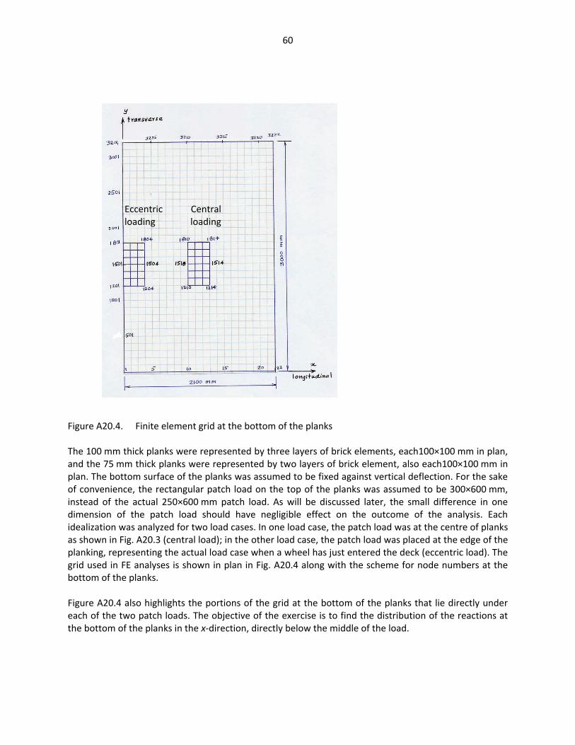
60

Figure A20.4. Finite element grid at the bottom of the planks The 100 mm thick planks were represented by three layers of brick elements, each100×100 mm in plan, and the 75 mm thick planks were represented by two layers of brick element, also each100×100 mm in plan. The bottom surface of the planks was assumed to be fixed against vertical deflection. For the sake of convenience, the rectangular patch load on the top of the planks was assumed to be 300×600 mm, instead of the actual 250×600 mm patch load. As will be discussed later, the small difference in one dimension of the patch load should have negligible effect on the outcome of the analysis. Each idealization was analyzed for two load cases. In one load case, the patch load was at the centre of planks as shown in Fig. A20.3 (central load); in the other load case, the patch load was placed at the edge of the planking, representing the actual load case when a wheel has just entered the deck (eccentric load). The grid used in FE analyses is shown in plan in Fig. A20.4 along with the scheme for node numbers at the bottom of the planks. Figure A20.4 also highlights the portions of the grid at the bottom of the planks that lie directly under each of the two patch loads. The objective of the exercise is to find the distribution of the reactions at the bottom of the planks in the x-direction, directly below the middle of the load.

Eccentric Central loading loading

61

The FE analyses were conducted for two sets of values of E. In one set, the values of E were different in the three directions, as noted above (orthotropic), and in the other set, the values of E were taken to be the same in all three directions (isotropic).

(a) (b)

Figure A20.5. Vertical nodal reactions at the bottom of the 100 mm thick planks under a central load: (a) planks with isotropic properties; (b) planks with orthotropic properties Reactions at the bottom of the 100 mm thick planks having isotropic and orthotropic properties and subjected to a central patch load are plotted in Figs. A20.5 (a) and (b), respectively, and the corresponding reactions under the 175 mm thick planks having isotropic and orthotropic properties are plotted in Figs. A20.6 (a) and (b), respectively. Comparisons of Figs. A20.5 (a) and (b), and Figs. A20.6 (a) and (b), will show that the dispersion of the load through the planks is not affected significantly by the properties of the planking. Following common wisdom, it was initially believed that the pressure at the bottom of the planks due a patch load would be significantly smaller than the pressure obtained by assuming a 45° distribution, illustrated in Fig. A20.1. Thicker planking should lead to better load dispersion and hence smaller pressure at the bottom of the planks were examined. To test this hypothesis, pressures due to the same load at the bottom of three different set of planks. One set of planks was 100 mm thick and had isotropic properties. The other two sets of planks were 170 mm thick, one with isotropic properties and the other with orthotropic properties. Nodal reactions at the bottom of the planks, which correspond to vertical pressure, are plotted in Fig. A20.7 along the x-axis (along node Nos. 1508 to 1516). As expected, the pressure is the highest under the centre of the 300 mm wide load, dropping off to zero some distance from the load. The width of the dispersed load at the bottom of the three planks, being approximately 700 mm, is larger than the 450 mm width obtained by 45° distribution (Fig. A20.1). However, it should be noted that in the 45° distribution, it is assumed that the dispersed load is distributed uniformly. The pressure distributions obtained by the FE analyses are highly non-uniform.

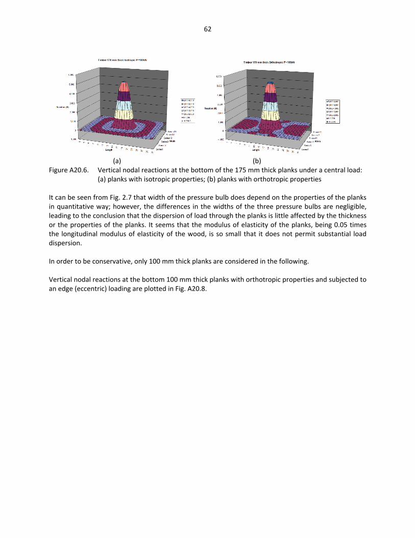
62

(a) (b) Figure A20.6. Vertical nodal reactions at the bottom of the 175 mm thick planks under a central load: (a) planks with isotropic properties; (b) planks with orthotropic properties It can be seen from Fig. 2.7 that width of the pressure bulb does depend on the properties of the planks in quantitative way; however, the differences in the widths of the three pressure bulbs are negligible, leading to the conclusion that the dispersion of load through the planks is little affected by the thickness or the properties of the planks. It seems that the modulus of elasticity of the planks, being 0.05 times the longitudinal modulus of elasticity of the wood, is so small that it does not permit substantial load dispersion. In order to be conservative, only 100 mm thick planks are considered in the following. Vertical nodal reactions at the bottom 100 mm thick planks with orthotropic properties and subjected to an edge (eccentric) loading are plotted in Fig. A20.8.

63

Figure A20.7. Vertical nodal reactions at the bottom of three different sets of planks under a central load

Figure A20.8. Vertical nodal reactions at the bottom of the 100 mm thick planks under an edge load

300 mm

t

t = 100 mm, isotropic plankt = 170 mm, orthotropic plank t = 170 mm, isotropic plank

Approx. 700 mm Distance along x-axis

N

odal

reac

tions

at b

otto

m o

f pla

nk

64

The actual and assumed equivalent uniformly distributed vertical pressures under the 100 mm thick planks are plotted in Figs. A20.9 (a) and (b) along the x-axis for the edge and central loads, respectively.

Figure A20.9. Vertical pressure at the bottom of the 100 mm thick plank: (a) edge load, (b) central load In Fig. A20.9 (a), the pressures obtained by FE analyses due to the edge load are assumed to be represented by (a) a rectangle curtailed by an inclined line, (b) a rectangle, and (c) by a triangle. The total areas of each of these shapes are nearly the same. Accordingly, the pressure within each shape is represented by a point load P/3 placed at the CG of the shape, where P is the total patch load. For the central load, the actual pressure is represented by two triangles and a rectangle. In this case also, the areas of the three shapes are nearly equal, so that the central load is represented by three point loads, each equal to P/3 placed at the CG of the respective shapes. Figures A20.9 (a) and (b) show the position of the point loads with respect to the load. As shown in Section 4, the end tie, which is closest to the abutment, experiences significantly higher load effects than its neighbours, because of which it important to model the wheel load as accurately as possible. Figures A20.10 (a) through (d) show different wheel positions in the left-hand sketches. In the right-hand sketches, the assumed pressure distributions are shown in the form of simple geometric shapes, as was done to develop the assumed pressure distributions in Figs. A20.9 (a) and (b). When the edge of a wheel just touches the edge of an end tie (Fig. A20.10 a), clearly there is no load applied to any tie. When the centre of a wheel is at the boundary of edge of an end tie and the approach slab (Fig. A20.10 b), the pressure on the ties can be represented by two point loads, the first being P/6 and the

100 100 100 100 100 100 mm

x-direction 50 110 120 145 120 120 mm

(a) (b)

FE analysis

Assumed

65

other P/3. When the wheel load is just inside the bridge (Fig. A20.10 c), the pressure can be represented by three point loads, each P/3. The wheel load can be considered to be fully inside the bridge when the edge of the pressure diagram just touches the boundary of the bridge and approach slab (Fig. A20.10 d).

Actual position of wheel Pressure at interface of planking and ties

Figure A20.10. Distribution of pressure at the interface of planks and ties due to different wheel positions For the three load cases shown in Figs. A20.10 (b) through (c), the distances of the point loads from the edge of the end tie are shown in Fig. 2.11 along with the fractions of the wheel load P apportioned to each point load. It is important to note that in Fig. A20.11 the distances of the point loads are noted with respect to the outer edge of the end tie. When the tie is idealized as a 1-dimensional element (as in the semi-continuum method), allowance should be made in the idealization for the half width of the tie.

(a) Wheel just outside the bridge (no pressure) (b) Centreline of wheel at the boundary of bridge and approach slab (c) Wheel just inside the bridge (d) Wheel inside the bridge with pressure edge at the boundary of bridge and applied slab

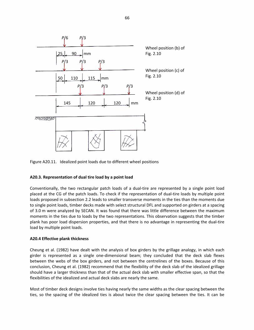
66

Figure A20.11. Idealized point loads due to different wheel positions

A20.3. Representation of dual tire load by a point load Conventionally, the two rectangular patch loads of a dual-tire are represented by a single point load placed at the CG of the patch loads. To check if the representation of dual-tire loads by multiple point loads proposed in subsection 2.2 leads to smaller transverse moments in the ties than the moments due to single point loads, timber decks made with select structural DFL and supported on girders at a spacing of 3.0 m were analyzed by SECAN. It was found that there was little difference between the maximum moments in the ties due to loads by the two representations. This observation suggests that the timber plank has poor load dispersion properties, and that there is no advantage in representing the dual-tire load by multiple point loads. A20.4 Effective plank thickness Cheung et al. (1982) have dealt with the analysis of box girders by the grillage analogy, in which each girder is represented as a single one-dimensional beam; they concluded that the deck slab flexes between the webs of the box girders, and not between the centrelines of the boxes. Because of this conclusion, Cheung et al. (1982) recommend that the flexibility of the deck slab of the idealized grillage should have a larger thickness than that of the actual deck slab with smaller effective span, so that the flexibilities of the idealized and actual deck slabs are nearly the same. Most of timber deck designs involve ties having nearly the same widths as the clear spacing between the ties, so the spacing of the idealized ties is about twice the clear spacing between the ties. It can be

Wheel position (b) of Fig. 2.10 Wheel position (c) of Fig. 2.10 Wheel position (d) of Fig. 2.10

P/6 P/3

25 90 mm

P/3 P/3 P/3

50 110 115 mm

P/3 P/3 P/3

145 120 120 mm

67

readily shown that for such cases, the effective thickness of the planking of the idealized semi-continuum should be about twice the actual thickness. The design checks, discussed in Section 4 will be conducted by using this assumption. A20.5. Conclusions The following conclusions are drawn.


• For all analyses to be conducted for the design check of timber decks, the two individual rectangular patch loads of a dual-tire are recommended to be idealized as a single point load placed at the CG of the two patch loads.


final report on design checks for timber decks on steel ... final report on design checks for timber...

Documents