i

Final Draft Report Contract #LPC80

2000

Determination of Properties and the Long Term Acceptance Rate of Effluents from Food Service

Establishments that Employ Onsite Sewage Treatment

Prepared By Brian C. Matejcek

Steve Erlsten &

Dr. David Bloomquist

Departments of Environmental Engineering Sciences and Civil & Coastal Engineering

University of Florida Gainesville, Florida 32611

For the Florida Department of Health

ii

TABLE OF CONTENTS

Page LIST OF TABLES iv LIST OF FIGURES vi ABSTRACT viii CHAPTER 1 INTRODUCTION 1 CHAPTER 2 LITERATURE REVIEW 3 Grease Interceptors 3 Septic Tank 4 Lift Station 6 Absorption Field 7 Aerobic Treatment Systems 12 System Failure 12

Phase I – An Examination of Restaurant OSTDS 15 CHAPTER 3 EXPERIMENTAL METHODS 19

Restaurant Characterization 20 Restaurant Selection 20 Restaurant Sampling 20 Analysis 21 Survey of Restaurants 23 Flow Data 23 Temperature and pH 24 Long Term Acceptance Rate Study 25 Lysimeter Construction 25

Soil Selection 28 Soil Properties 29

Soil Location 30 Soil Collection 31 Packing of Soil Columns 32 Experimental Control Lysimeters 35 Hydraulic Conductivity 35 Synthetic Wastewater 37 Synthetic Wastewater Batch 39 Dosing 40 Measurements 40

iii

CHAPTER 4 RESULTS AND DISCUSSION 42 Restaurant Effluent Characterization 42 Long Term Acceptance Rate Study 61 Synthetic Wastewater 62 Column Failure 64 One-foot unsaturated columns 68 Two-foot unsaturated columns 71 Column Effluent Sampling 80 CHAPTER 5 SUMMARY, CONCLUSIONS AND RECOMMENDATIONS 93 Summary 93 Conclusions 93 Recommendations 94 REFERENCES 96 APPENDIX A SOIL DENSITY DATA 99 APPENDIX B STANDARD OPERATING PROCEDURES 127 APPENDIX C RESTAURANT TEMPERATURE AND pH DATA 138 APPENDIX D RESTAURANT SURVEYS 145 APPENDIX E RESTAURANT SITE PLANS 158

iv

LIST OF TABLES Table Page 2-1. Estimated Sewage Flows for Restaurants 5 2-2. Septic Tank and Pump Tank Capacity for Restaurants 6 2-3. Soil Criteria for Absorption Fields 8 2-4. Food Service Establishment Categories 16 2-5. Analytical Results For Each Restaurant Category 18 3-1. Moisture Content and Analysis Percent Recovery 38 3-2. Synthetic Wastewater Concentrations 38 3-3. Synthetic Wastewater Mass Requirements 40 4-1. Restaurant Sample Collection 43 4-2. Analytical Results For Carbonaceous Biochemical

Oxygen Demand 53 4-3. Analytical Results For Total Suspended Solids 53 4-4. Analytical Results For Oil and Grease 54 4-5. Target Concentrations for Synthetic Wastewater 63 4-6. Synthetic Wastewater Concentrations 63 4-7. Mean Days to Failure For Two-Foot Unsaturated Columns 74 4-8. Total Mass Loading of Candler Soil Series for Two Feet

of Unsaturated Soil 78 4-9. Daily Mass Loading of Candler Soil Series for Two Feet

of Unsaturated Soil 78 4-10. Total Mass Loading of Millhopper Soil Series for Two Feet

of Unsaturated Soil 78 4-11. Daily Mass Loading of Millhopper Soil Series for Two Feet

of Unsaturated Soil 79

v

4-12. Total Mass Loading of Pomona Soil Series for Two Feet of Unsaturated Soil 79

4-13. Daily Mass Loading of Pomona Soil Series for Two Feet

of Unsaturated Soil 79

4-14. Total Mass Loading of Pomona with Candler Fill Soil Series for Two Feet of Unsaturated Soil 80

4-15. Daily Mass Loading of Pomona with Candler Fill Soil

Series for Two Feet of Unsaturated Soil 80

4-16. CBOD5 Column Effluent Low Strength 87 4-17. CBOD5 Column Effluent Medium Strength 88 4-18. CBOD5 Column Effluent High Strength 89 4-19. TSS Column Effluent Low Strength 90 4-20. TSS Column Effluent Medium Strength 91 4-21. TSS Column Effluent High Strength 92

vi

LIST OF FIGURES

Figure Page 2-1. Cross-section of a Standard Trench Drainfield System 9 2-2. Cross-section of a Mound Drainfield System 11 3-1. Lysimeter Design 26 3-2. Soil Profiles for Lysimeter 34 4-1. Effluent Concentrations from Site 1 45 4-2. Effluent Concentrations from Site 2 45 4-3. Effluent Concentrations from Site 3 46 4-4. Effluent Concentrations from Site 4 46 4-5. Effluent Concentrations from Site 5 47 4-6. Effluent Concentrations from Site 6 47 4-7. Effluent Concentrations from Site 7 48 4-8. Effluent Concentrations from Site 8 48 4-9. Effluent Concentrations from Site 9 49 4-10. Effluent Concentrations from Site 10 49 4-11. Effluent Concentrations from Site 11 50 4-12. Effluent Concentrations from Site 12 50 4-13. Effluent Concentrations from Site 13 51 4-14. Effluent Concentrations from Site 14 51 4-15. Effluent Concentrations from Site 15 52 4-16. Categorization of CBOD5 Concentration per Site 56 4-17. Categorization of TSS Concentration per Site 57

vii

4-18. Categorization of O&G Concentration per Site 58 4-19. Column Failure for Low Strength Wastewater 65 4-20. Column Failure for Medium and High Strength Wastewater 67 4-21. Volumetric Water Content of Soils 70 4-22. Days to Failure versus Wastewater Loading Rate 75 4-23. Days to Failure versus Mass Loading of Medium Strength Wastewater 76 4-24. Days to Failure versus Mass Loading of High Strength Wastewater 76 4-25. Days to Failure versus Mass Loaded 77 4-26. Air Temperature during LTAR Study 83 4-27. Percent Relative Humidity in Room Air 84

viii

ABSTRACT

DETERMINATION OF PROPERTIES AND THE LONG TERM ACCEPTANCE RATE

OF EFFLUENTS FROM FOOD SERVICE ESTABLISHMENTS THAT EMPLOY

ONSITE SEWAGE TREATMENT

Restaurants in Florida have problems in disposing of their high-strength wastes using onsite treatment and disposal systems, with failures occurring regularly. This study is part of the program designed to determine the characteristics of the wastes being generated and to establish possible solutions. This report gives the results of the testing done to characterize the effluents and then develop a synthetic wastewater for use in subsequent tests. Those tests were designed to determine the long-term acceptance rates for typical soils using practical loading protocols. Several recommendations for solving the disposal problems are presented. The physical and chemical characteristics of the septic tank effluents from fifteen randomly chosen restaurants were determined using a total of 133 samples collected between May 1997 and March 1999. Levels were established for the five-day carbonaceous biochemical oxygen demand (CBOD5), total suspended solids (TSS), and oils and greases (O&G). The effluents were sorted into high-, medium-, and low-strength categories as standards for the long-term acceptance rate (LTAR) study that followed. The low-strength category was comparable in strength to that of effluents from residential septic tank systems. This information was used to prepare non-hazardous artificial wastewater suspensions with physical and chemical characteristics that approximated those of the actual restaurant wastewaters. The LTAR study used four common Floridian soil types in testing columns (lysimeters) that were designed to simulate drainfield conditions. Artificial wastewater of three strengths was applied under two saturation conditions that simulated those found in restaurants until failure occurred. These failures were due to the physical and biological clogging of the soil infiltration surface and varied widely, depending primarily on the mass loading rates. Failure occurred primarily in the lysimeters with two feet of unsaturated soil that were dosed with high- and medium-strength wastewater. Twenty-four lysimeters failed during the 112-day study with 20 failures occurring between days 20 and 47. No failures were recorded in lysimeters with low strength wastewater, which received a daily mass loading of 0.0015 lb/ft2/day or less. In addition, total mass loaded on the low strength soil columns has exceeded the mass loading of the failed columns dosed with medium strength wastewater.

1

CHAPTER 1

INTRODUCTION

Onsite sewage treatment systems (OSTDS) are the primary means for wastewater

treatment and disposal in areas outside of municipality boundaries. The Florida Onsite

Wastewater Association (FOWA) reported 36,221 OSTDS installations in the State of

Florida in 1996-97 and 35,237 system installations in 1997-98. In addition there were a total

of 19,852 and 20,927 repair permits issued in those same respective years by the Florida

Department of Health (FDOH). Actual system failures and the potential for system failures

have increased concern for surface- and ground-water contamination as well as for other

public health issues. Study emphasis has been placed on commercial OSTDS, including food

service establishments (FSE) or restaurants, because of high wastewater flows and higher

waste strength potentials.

Restaurant OSTDS have significantly higher failure rates than domestic systems.

Effluent quality of restaurants may have 2.8 times the concentration of biochemical oxygen

demand (BOD) and total suspended solids (TSS) compared to domestic systems (Siegrist et

al., 1984). In a Wisconsin study (Siegrist et al., 1984), two restaurants experienced hydraulic

failure within months after installation. In comparison, the mean age to failure for residential

OSTDS in Florida is approximately 18 years (Sherman et al., 1998). Although higher

wastewater strengths induce faster absorption field (drainfield) failures and different

establishments vary in strength of waste produced, system designs used for disposal do not

2

vary among establishments. Because restaurant treatment systems are designed based on

criteria used for lower strength residential wastes, restaurant owners face economic

consequences of drainfield failure along with public health issues. The cost of absorption

field replacement can range between $4.00/ft2 to $12/ft2 of drainfield (personal

correspondence with Florida Septic, Inc., 2000).

The failure of these fields not only represents a serious public health hazard but also

may impact ground and surface waters with biological and chemical pollutants (Alhajjar,

1990). Nutrient overloading and BOD in waterways contributes to the degradation of water

quality. Nitrogen and phosphorus can lead to eutrophication of water. High BOD

concentrations can deplete oxygen levels in receiving waters leading to fish kills and

anaerobic conditions. When failure occurs, humans could be exposed to pathogenic

microorganisms such as Salmonella, Shigella, Giardia and viruses in the untreated

wastewater (Yates, 1989).

Chapter 64E-6 of the Florida Administrative Code (FAC) regulates the design of

onsite sewage treatment and disposal systems (OSTDS). There are over 1.6 million

residences and commercial establishments in the State of Florida that use OSTDS as the

primary means for wastewater disposal. Current design codes are based on estimates of daily

flows, but differences between the wastewater strengths and organic loadings for domestic

and restaurant effluent are not taken into consideration.

3

CHAPTER 2

LITERATURE REVIEW

Conventional OSTDS are composed of two primary components: the septic tank and

the absorption drainfield. The septic tank allows solids to settle, separates floating debris

(scum) from the waste stream and acts as an anaerobic digester (Metcalf and Eddy, 1991).

The drainfield provides final aerobic treatment of the wastewater effluent and is the single

disposal method of wastewater generated onsite. Restaurant OSTDS include a grease

interception tank, where one or more tanks may be placed in series prior to the septic tank.

Effluent exits the gravity flow system to the drainfield or into a holding tank (lift station)

from which wastewater is pumped to the absorption drainfield.

Grease Interceptors

Grease interceptors (grease traps) are required for all commercial establishments

(facilities other than domestic residences) “where grease is produced in quantities that could

otherwise cause line stoppage or hinder sewage disposal” (FAC, Chapter 64E-6.013).

Additionally, grease traps may be required for restaurants where suspended solids may be

produced in excessive quantities (personal correspondence from Paul Myers, FDOH). Grease

traps are essentially modified septic tanks and act as heat exchangers (Metcalf and Eddy,

1991). The baffled tank traps oil and grease by cooling the water, solidifying the grease and

preventing floating oils from exiting the tank (Metcalf and Eddy, 1991). Grit and suspended

4

solids also settle in the tank. The equation to determine the minimum capacity of the grease

interceptor is given (FAC, Chapter 64E-6.013):

Grease interceptor capacity (gallons) = (S) x (GS) x (HR/12) x (LF)

where: S = number of seats in the dining area, GS = gallons of wastewater per seat (10 gal. for single service

restaurant or 25 gal. for all other), HR = hours of operation, LF = loading factor (2.0 interstate highways, 1.5 other freeways, 1.25 recreational areas, 1.0 main highways, and 0.75 other).

The minimum and maximum tank volumes of grease interceptors are 750 and 1250

gallons. If the required capacity exceeds 1250 gallons, several grease traps may be placed in

series. Failure to capture grease and oil from effluent can cause pump tank malfunction, pipe

blockage and drainfield clogging.

Septic Tank

A septic tank is, by definition, “a watertight receptacle constructed to promote

separation of solid and liquid components of wastewater, to provide limited digestion of

organic matter, to store solids, and to allow clarified liquid to discharge for further treatment

and disposal into a drainfield” (FAC, Chapter 64E-6). Oxygen is quickly utilized by

microorganisms in the septic tank, leaving settled material to undergo anaerobic

decomposition. Baffles in the tank prevent the floating scum layer (oil, grease and solids)

from exiting the tank. Septic tank sizing is based upon the estimated daily flow of the

establishment. The criteria used to estimate the daily effluent flow of restaurants is located in

Table 2-1. The estimated flows are then used to find the effective septic tank capacity.

However, as wastewater flows increase, the minimum effective septic tank capacities do not

5

increase linearly (Table 2-2). The resulting detention time of septic tanks therefore decrease

as wastewater flow increases (see below example). The capacity information is given in

Table 2-2.

Example: A 100-seat, full service restaurant operating for less than 16 hours would

have an estimated flow of 4000 gallons/day (Table 2-1). The minimum septic volume

required for a flow of 4000 gallons/day is 4800 gallons (Table 2-2), giving a detention time

of 1.2 days (volume divided by flow). However, a domestic system with 200 gallons/day of

flow requires a 900-gallon septic tank, resulting in a detention time of 4½ days.

Table 2-1. Estimated Sewage Flows for Restaurants (FAC, Chapter 64E-6.008, Table I)

Food Operation Estimated Gallons Per Day Per Seat

a) Restaurant operating 16 hours or less per day per seat 40 b) Restaurant operating more than 16 hours per day per seat 60 c) Restaurant using single service dishware only and operating 16 hours or less per day per seat

20

d) Restaurant using single service dishware only and operating more than 16 hours per day per seat

35

e) Bar and cocktail lounge per seat; add per pool table or video game

20 15

f) Drive-in restaurant per car space 50 g) Carry out only, including caterers: 1. per 100 square feet of floor space 2. add per employee per 8 hour shift

50 15

h) Institutions per meal 5 i) Food outlets excluding deli, bakery or meat department 1. per 100 square feet of floor space 2. add for deli per 100 sq. ft. of deli floor space 3. add for bakery per 100 sq. ft. of bakery space 4. add for meat dept. per 100 sq. ft. of meat dept. floor space 5. add per water closet

10 40 40 75 200

6

Table 2-2. Septic Tank and Pump Tank Capacity for Restaurants (Adopted from FAC, Chapter 64E-6.008, Table II)

Average Septic Tank Pump TankSewage Minimum Minimum

Flow Effective EffectiveCapacity Capacity

(Gallons/day) (Gallons) (Gallons)0-200 900 225

201-300 900 375301-400 1050 450401-500 1200 600501-600 1350 600601-700 1500 750701-800 1650 900801-1000 1900 10501001-1250 2200 12001251-1750 2700 19001751-2500 3200 27002501-3000 3700 30003001-3500 4300 30003501-4000 4800 30004001-4500 5300 30004501-5000 5800 3000

Lift Station

Automatic dosing systems are required for commercial establishments when the flow

is greater than 500 gpd or if the area of the drainfield is greater than 1000 square feet (FAC,

Chapter 64E-6). Lift stations (also referred to as pump tanks or pumping chambers) are also

necessary in situations where wastewater must be elevated to overcome gravity as with

mound systems (description later in this chapter). A lift station consists of a storage tank and

an automatic dosing device, which discharges effluent to an absorption field. Sizing of lift

stations depends on the dose volume, total dynamic head (elevation), desired flow rate and

7

wastewater characteristics (EPA, 1980). Commercial tanks must have at least two alternating

pumps with water level controls. The lift station must be sized so the entire drainfield

receives effluent during the dosing period. This insures that the entire drainfield is utilized

for treatment and disposal instead of individual sections.

Absorption Field

The absorption field, commonly known as a drainfield, provides the final treatment

and disposal of the effluent from the OSTDS. Effluent treatment in a drainfield is a

combination of physical, chemical and biological treatment. The main components of a

drainfield include a series of shallow trenches filled with a porous media or aggregate

(gravel), which surrounds a distribution pipe (Viessman and Hammer, 1993). The bottom of

the trench is filled with a 6- to 10-inch layer of porous media (aggregate), and a single

distribution pipe is laid. Then it is encased in the porous media (porous media has a

minimum thickness of 12 inches). The distribution lines (usually a 4-inch minimum inner

diameter pipe with two rows of holes or perforations) and porous media distribute the

OSTDS effluent over the entirety of the drainfield (FAC, Chapter 64E-6.014). A membrane

composed of polyester bonded filament covers each trench and prevents intrusion of the

backfilled soil (drainfield soil cover) into the porous media.

Soil below the drainfield must have an effective depth of at least 42 inches of slightly

limited or moderately limited soil (suitable soil). Slightly limited soils include sand, loamy

sand and fine sand with a rapid percolation (1 to 4 min/inch). Moderately limited soils

include sandy loam, fine sand loam and very fine sand with a moderate percolation (5 to 10

min/inch). Clay loam, sandy clay and silt with percolation rates between 15 and 30 min/inch

8

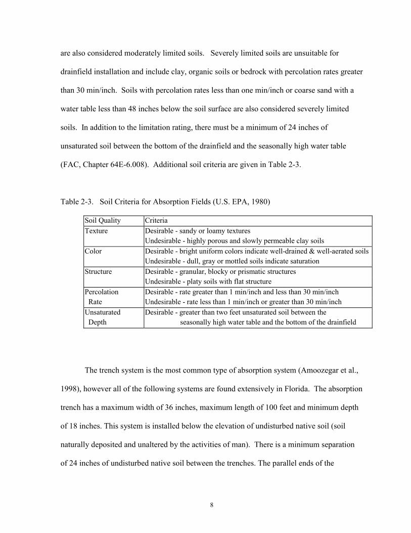
are also considered moderately limited soils. Severely limited soils are unsuitable for

drainfield installation and include clay, organic soils or bedrock with percolation rates greater

than 30 min/inch. Soils with percolation rates less than one min/inch or coarse sand with a

water table less than 48 inches below the soil surface are also considered severely limited

soils. In addition to the limitation rating, there must be a minimum of 24 inches of

unsaturated soil between the bottom of the drainfield and the seasonally high water table

(FAC, Chapter 64E-6.008). Additional soil criteria are given in Table 2-3.

Table 2-3. Soil Criteria for Absorption Fields (U.S. EPA, 1980)

Soil Quality Criteria Texture Desirable - sandy or loamy textures

Undesirable - highly porous and slowly permeable clay soils Color Desirable - bright uniform colors indicate well-drained & well-aerated soils

Undesirable - dull, gray or mottled soils indicate saturation Structure Desirable - granular, blocky or prismatic structures

Undesirable - platy soils with flat structure Percolation Desirable - rate greater than 1 min/inch and less than 30 min/inch Rate Undesirable - rate less than 1 min/inch or greater than 30 min/inch Unsaturated Desirable - greater than two feet unsaturated soil between the Depth seasonally high water table and the bottom of the drainfield

The trench system is the most common type of absorption system (Amoozegar et al.,

1998), however all of the following systems are found extensively in Florida. The absorption

trench has a maximum width of 36 inches, maximum length of 100 feet and minimum depth

of 18 inches. This system is installed below the elevation of undisturbed native soil (soil

naturally deposited and unaltered by the activities of man). There is a minimum separation

of 24 inches of undisturbed native soil between the trenches. The parallel ends of the

9

perforated distribution pipes are perpendicularly connected to form a continuous circuit

(FAC, Chapter 64E-6.014). Figure 2-1 displays only one of the multiple trenches that

compose a trench system drainfield.

Figure 2-1. Cross-section of a Standard Trench Drainfield System

An absorption bed can be constructed in lieu of an absorption trench, which is

essentially a wide trench with multiple effluent distribution lines. The entire soil content of

the bed is removed and replaced with a porous media (EPA, 1980). Distribution lines are

placed on the porous media with a 36-inch maximum separation between lines and a

maximum infiltration area of 1500 ft2 (FAC, Chapter 64E-6.014). The lack of “sidewalls”

(trench minimum depth of 12 inches) between each distribution line can reduce the available

soil infiltration surface area by a factor of five when compared to absorption trenches. Thus

trench systems are the preferred method of effluent disposal. Absorption beds require less

10

total land area than trench systems (EPA, 1980). However, the maximum allowable sewage

loading rate for absorption beds is reduced by 20% to 45% (depending on soil texture)

compared to the loading rate of an equivalent trench system (FAC Chapter 64E-6.008).

A second type of absorption field is called a mound system. Mound systems are

required for severely limited soils (poorly drained soils) and where the seasonally high water

table is too near the ground surface (EPA, 1980). These systems are trench or bed systems

that have been raised above the ground surface elevation with the use of fill material. Fill

material consisting of moderately limited or slightly limited soil (usually sand or fine sand) is

transported and placed above the existing native soil until a predetermined elevation is

reached (Metcalf and Eddy, 1991). There must be at least 42 inches of suitable soil below

the bottom of the drainfield and a minimum of 24 inches of unsaturated soil above the

seasonally high water table (EPA, 1980). The porous media and distribution line network is

laid in a similar manner to the trench or bed systems and the mound system is capped with a

minimum of 9 inches of fill material. The maximum allowable sewage loading rate for

mound systems is reduced by 16% to 27% (depending on soil texture) compared to the

loading rate of an equivalent trench or bed system. The side slopes of a 36-inch mound

drainfield are two feet horizontal for each vertical foot. Slopes for mounds greater than 36

inches high are 3:1 (FAC, Chapter 64E-6.009).

Mound systems are more costly to install than standard subsurface systems due to the

purchase and transportation of fill material. Costs also may include the addition of a lift

station, which is often required to pump effluent to mound systems because of the raised

elevation of the drainfield. Figure 2-2 illustrates the location of the ground surface with

11

respect to the drainfield, however the actual heights of subsurface suitable and unsuitable

soils will vary between sites.

Figure 2-2. Cross-section of a Mound Drainfield System

A filled system is a variation on the mound system. In this case, “a portion, but not

all, of the drainfield sidewalls are located at an elevation above the elevations of undisturbed

native soil” (FAC, Chapter 64E-6.002). In this case, unsuitable soils in terms of texture or

permeability are excavated and replaced with fill material. These systems are designed in

accordance with the minimum requirements for mound systems. Filled systems require less

land space when compared to mound systems due to the reduced height and reduction of the

corresponding side slope. In addition, filled systems can receive the equivalent maximum

allowable sewage loading rates as absorption trench and bed systems, which are greater than

the allowable sewage loading rates to mound systems (FAC, Chapter 64E-6.009).

12

Aerobic Treatment Systems

Alternative systems to conventional septic tanks have typically focused on aeration.

Generally air is bubbled through the wastewater effluent to maintain aerobic conditions.

Aerobic digestion is more efficient than anaerobic with increased uptake of BOD (Bitton,

1994). Statewide there were 1,161 aerobic permits in 1996-97 and 1,222 in 1997-98 issued

by FDOH (FOWA, 1999). Several variations of aerobic systems are manufactured, including

the Nibbler� system, which was utilized at two restaurant sites in the study.

The Nibbler� is an aerobic digester pretreatment system that treats high strength

wastewater and is capable of accepting “shock loads” during peak flow times. The system

uses aeration to up-flow wastewater through submerged buoyant media in the unit (Sluth,

1989). Waste strength levels are reduced to concentrations found in residential OSTDS.

System Failure

A drainfield system is designed to distribute effluent for filtration, oxidation,

reduction and absorption by the soil. System failure is the discharge of untreated (or

inadequately treated) wastewater into the environment, including discharge to the ground

surface, ground water or surface waters (FAC, Chapter 64E-6.002). Drainfield failure

specifically refers to the clogging of the drainfield by either or both physical clogging or

biological interference. Characteristic initial indicators include reduced water flow from the

restaurant. Later indicators of failure include ponding over the drainfield, sewage

overflowing from tanks and wastewater backing up into buildings.

13

Physical clogging of the drainfield occurs when suspended solids, sludge, oils and

grease reach the drain field. These particles collect on the soil infiltration surface and limit

water permeability through the soil. The oils and grease not collected in the grease

interceptor can pose severe problems in the drainfield because of their persistence.

A biological clogging mat or biomat forms on the porous media and infiltration

surface of the drainfield after the system has been in service for some time. The biomat is

both a physical and biological filter and treats effluent for BOD and TSS as it passes over the

biomat (Metcalf and Eddy, 1991). Biomat thickness ranges from 0.7-cm to 2.5-cm in the soil

and attaches to the porous media below the perforated distribution pipe (May, 1996). The

biomat thickness will increase as the microorganisms metabolize the depositing organics in

the effluent. However, the permeability of the soil at the infiltration layer is greatly decreased

by this process. The hydraulic capacity of the drainfield becomes a function of the biomat

rather than a result of the hydraulic characteristics of the soil (Metcalf and Eddy, 1991).

Effluent flow to the drainfield can be gravity flow or by periodic doses by a pump. In

gravity flow systems wastewater intermittently flows to the drainfield, resulting in locally

distributed anaerobic (absence of molecular oxygen) regions due to saturation. A heavy and

uniform biomat is formed due to these conditions. The biomat attached to the soil surface and

drainfield aggregate supporting the perforated distribution pipe “acts as a submerged

anaerobic filter” metabolizing organic materials into methane and carbon dioxide (Metcalf

and Eddy, 1991). Effluent is constantly entering the system, leaving the infiltration soil

surface saturated. However, the vadose zone (unsaturated zone between the ground surface

and water table) remains aerobic due to the slow infiltration of effluent through the biomat.

14

Periodic dosing is usually aerobic and the biomat attached to the drainfield aggregate

“acts as a trickling filter”(Metcalf and Eddy, 1991). Dosing provides better wastewater

distribution over the entire drainfield, which allows for more efficient treatment, compared to

intermittent gravity flow systems. In addition the biomat is more evenly distributed

throughout the drainfield but is thinner than with intermittent flow (Metcalf and Eddy, 1991).

Under aerobic conditions, microorganisms digest the organic matter and convert it to carbon

dioxide, water and other inert materials. Effluent treatment is more rapid under aerobic

conditions when compared to anaerobic biological treatment (Metcalf and Eddy, 1991).

The infiltration surface includes not only the soil below the perforated distribution

line but also the sidewalls of the trench system. Wastewater infiltrates the drainfield

sidewalls, and the biomat will continue to form on the trench walls and adjacent porous

media. System longevity becomes a function of the effluent loading rate, sidewall height

(depth of the trench) and clogged soil infiltration rate (Keys et al., 1998). In addition, the

formation of the biomat is a function of wastewater loading: increasing the organic loading

tends to accelerate the biomat growth (Amoozegar, 1998).

For soils high in clay mineral content, reduction of the soils infiltration capacity can

be severely reduced during drainfield installation (Uebler, 1984). Digging with a backhoe

can cause “soil smearing” or a reorientation of the soil particles, which reduces the soils

absorptive capacity compared to the undisturbed conditions (Uebler, 1984).

Problems observed with sizing OSTDS based primarily on hydraulic loading are that

the effluent quality and resulting mass loading is not taken into consideration for drainfield

design. This increased waste strength has been shown in previous studies to have significant

impact on the performance of an OSTDS and may shorten the life of the system. The purpose

15

of this study is to determine the effects of wastewater strength (constituent concentration) on

drainfield absorption systems. Concentrations of biochemical oxygen demand (CBOD5),

total suspended solids (TSS), and oils and grease in the effluents of operating restaurants

determine effluent strength. The average effluent concentrations for these three parameters

are significantly higher for restaurants than they are for residences.

Phase I - An Examination of Restaurant OSTDS

The research presented in this report is the second phase of a two-phase restaurant

OSTDS study. The conception and completion of this research was a direct result of

recommendations and conclusions derived from the first phase. This research was initiated in

January 1997 and was completed in June 2000 and is the main focus of this report. Phase I of

the research began in January 1996 and was completed in January 1997 (Waters, 1998) and is

summarized below.

Phase I of the study investigated several effluent properties from food service

establishments (FSE) that employ onsite sewage treatment and disposal systems (OSTDS).

Septic tank effluent from a total of 19 restaurants was sampled in Alachua and surrounding

counties in North Central Florida. Each restaurant was sampled twice and analyzed for 5-day

biochemical oxygen demand (EPA Method 405.1), total suspended solids (EPA Method

160.2) and n-hexane extractable oils and grease (EPA Method 1664). Additional qualitative

analyses using a gas chromatograph and mass spectrometer (GCMS) were run to determine

the presence of trace organics from degreasers and cleaning agents (EPA Method 625). Soil

borings from each site were examined to determine the suitability of soil to accept septic tank

effluent.

16

The State of Florida Department of Health and Rehabilitative Services provided a list

of 161 restaurants operating in North Central Florida. The restaurants were divided into

eight categories (Table 2-4). The original hypothesis was that restaurant category might be

an indicator of effluent quality.

Table 2-4. Food Service Establishment Categories

Category Restaurant Type 1 Restaurants operating less than 16 hours per day 2 Single Service restaurants operating less than 16 hours per day 3 Single Service restaurants operating more than 16 hours per day 4 Bars and cocktail lounges 5 Drive in restaurants 6 Food outlets 7 Bakeries 8 Convenience Stores

Restaurants selected for this study were operating an OSTDS and permission had

been granted by the owner/manager to participate in the study. Limitations for collection of

effluent samples included travel distance, and the time and budget limitations set for Phase I.

Each effluent sample was collected from a location immediately prior to discharge to

the septic tank drainfield. A number of restaurants used lift stations, which are holding tanks

located after the septic tanks and prior to the drainfields. Floats in a lift station activate

pumps when the septic tank effluent reaches a predetermined level, and the effluent is then

pumped into the drainfield. Florida Septic Inc., a septic tank installer/contractor for

restaurant OSTDS, installed sampling ports between the septic tank and drainfield for

restaurants without lift stations. Grab samples (approximately 4 liters each) were taken from

each restaurant and analyzed for 5-day biochemical oxygen demand (BOD), total suspended

17

solids (TSS) and oils and grease (O&G). In addition, samples were collected and analyzed

for trace organics using EPA Method 625 for both the extraction and analysis (Waters, 1998).

The BOD5, TSS and O&G analyses were selected to quantify effluent quality of

OSTDS-treated wastewater. BOD5 gives a general indication of the amount of biodegradable

matter in the effluent. TSS determines the concentration of suspended solids in solution.

O&G determines the amount of n-hexane extractable material (HEM) in the sample. HEM

includes non-volatile hydrocarbons, vegetable oils, animal fats, waxes, greases and similar

materials.

Results from the laboratory analyses of the 38 samples (two grab samples from each

restaurant) varied greatly between sites, restaurant categories and sampling events. BOD5

values ranged from 103 mg/L to 2820 mg/L, TSS concentrations ranged from 40 mg/L to

4775 mg/L and O&G concentrations ranged from 10 mg/L to 300 mg/L (Waters, 1998).

Analyses using the GCMS (EPA Method 625) showed no detectable levels of toxic organics

from cleaning products, nor were any compounds detected that might inhibit anaerobic

activity or negatively impact effluent characteristics.

The two main statistical evaluations that were completed on the data were the

Analysis of Variance (ANOVA) and the Duncan Multiple Range Test. The Duncan analysis

is a measurement of the sample size required to detect a statistical difference between two

categories that are a given number of standard deviations apart and carried out for various

error values (alpha and beta). The results of all the restaurant data collected in the respective

categories and statistically analyzed using the ANOVA procedure are listed in Table 2-5.

18

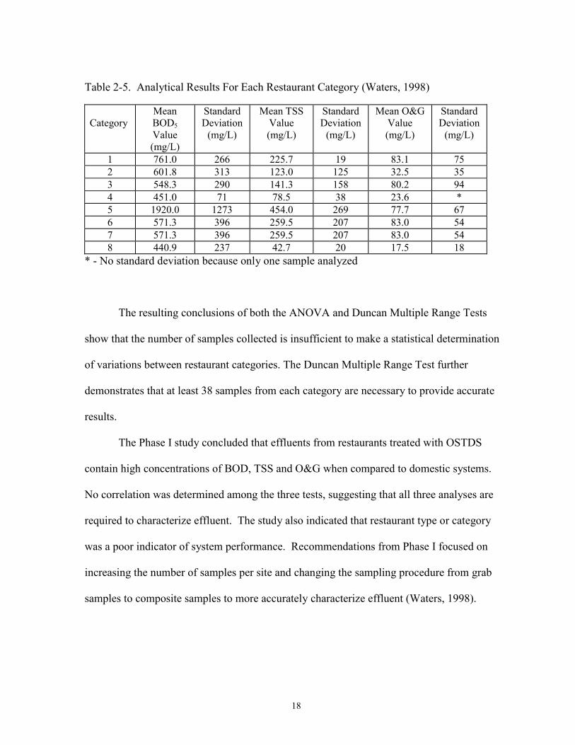
Table 2-5. Analytical Results For Each Restaurant Category (Waters, 1998)

Category

Mean BOD5 Value (mg/L)

Standard Deviation

(mg/L)

Mean TSS Value (mg/L)

Standard Deviation

(mg/L)

Mean O&G Value (mg/L)

Standard Deviation

(mg/L)

1 761.0 266 225.7 19 83.1 75 2 601.8 313 123.0 125 32.5 35 3 548.3 290 141.3 158 80.2 94 4 451.0 71 78.5 38 23.6 * 5 1920.0 1273 454.0 269 77.7 67 6 571.3 396 259.5 207 83.0 54 7 571.3 396 259.5 207 83.0 54 8 440.9 237 42.7 20 17.5 18

* - No standard deviation because only one sample analyzed

The resulting conclusions of both the ANOVA and Duncan Multiple Range Tests

show that the number of samples collected is insufficient to make a statistical determination

of variations between restaurant categories. The Duncan Multiple Range Test further

demonstrates that at least 38 samples from each category are necessary to provide accurate

results.

The Phase I study concluded that effluents from restaurants treated with OSTDS

contain high concentrations of BOD, TSS and O&G when compared to domestic systems.

No correlation was determined among the three tests, suggesting that all three analyses are

required to characterize effluent. The study also indicated that restaurant type or category

was a poor indicator of system performance. Recommendations from Phase I focused on

increasing the number of samples per site and changing the sampling procedure from grab

samples to composite samples to more accurately characterize effluent (Waters, 1998).

19

CHAPTER 3

EXPERIMENTAL METHODS

The purpose of the study was to monitor selected effluent properties from food

service establishments (FSE) that employ onsite sewage treatment and disposal systems

(OSTDS) and to conduct a long-term acceptance rate study (LTAR). A total of 15

restaurants were sampled in Alachua and surrounding counties in North Central Florida.

Eight samples were collected from each restaurant and analyzed for CBOD, TSS and O&G.

The LTAR laboratory study consisted of triplicate lysimeters packed with four typical soil

types commonly found in Florida, two saturation conditions and dosed with one of three

categories of wastewater strength determined from the field data. This research (Phase II)

was initiated in January 1997 and was completed in June 2000.

The Florida Department of Health entered into a contract (LPC80) with the

University of Florida to complete Phase II of the restaurant study. The first eight tasks of the

contract refer to collection of effluent samples, the analyses of those samples and the final

characterization of the restaurant effluent samples. The specific tasks included: 1) purchase

of equipment, 2) determination of 15 food service establishments, 3) formulation of a

sampling plan, 4) obtaining or creating site plans, 5) survey of FSE operations, 6) collection

of eight effluent samples from 15 restaurants and analyzing for CBOD5, TSS and O&G, 7)

20

collection flow, pH and temperature data, and 8) categorization of food operation wastewater

effluent into three strength categories.

Contract tasks 9, 10 and 11 deal specifically with the lysimeter study. Task 9

provides for the determination of the four soil types to be used in the long-term acceptance

rate (LTAR) study that are representative of soils commonly used in the state for drainfields.

Task 10 specifies the lysimeter design and experimental conditions with three wastewater

strength levels, four soil types, two saturation conditions and triplicate columns. Task 11 is

the implementation of the LTAR study with the response variable in days to failure.

Restaurant Characterization

Restaurant Selection

Seven of the 19 restaurants sampled in Phase I also participated in Phase II. The

Phase I site numbers were 1,4, 6, 9, 11, 13 and 19 and were changed in Phase II to numbers

6, 7, 8, 4, 3, 9 and 10, respectively. The additional eight sites were chosen randomly from a

list of restaurants operating in North Central Florida, which was provided by the State of

Florida Department of Health.

Restaurant Sampling

Sample collection changed from a single grab sample used in Phase I (Waters, 1998)

to a 24-hour composite sample based upon recommendations from the first study. This was

accomplished using an ISCO Portable Sampler. This device produces a 300-ml sample

suctioned by the sampler’s peristaltic pump every hour for a 24-hour period and deposited

into a 2.5 gallon Nalgene composite bottle. Prior to setup at the site, the composite bottle

21

was surrounded by ice for sample preservation. A vinyl suction line attached to a weight

with a stainless steel strainer was dropped into the lift station and adjusted until the strainer

was at mid depth between the tank bottom and water surface. The lift station manhole cover

was then returned with one side straddling a wood block to prevent pinching of the sampling

hose. The ISCO sampler was activated and then locked securely on-site. All restaurants'

OSTDS in this phase of the research had lift stations to allow easy access for sampling.

The sampling crew installed the sampler at a location and returned the following day

to retrieve the equipment. The composite container was shaken to thoroughly mix the

composite sample and re-suspend any solids that had settled since collection. Using 1-liter

amber sample jars, samples were collected and iced for the return trip to the UF Water

Chemistry Lab.

Analyses

Samples were collected for the same three analyses as in Phase I with one minor

exception. The biochemical oxygen demand (BOD) was modified to carbonaceous

biochemical oxygen demand (CBOD5) using a nitrification inhibitor to prevent any oxygen

loss during the five-day test due to the nitrification process. The resulting oxygen depletion

would be solely the result of microorganisms respiring. The two remaining analyses, total

suspended solids (TSS) and oils and grease (O&G), remained unchanged. Standard operating

procedures of each for the analyses are detailed in Appendix B from Waters (1998).

CBOD5 and TSS were the first two tests run because of the 48-hour and one-week

respective holding times compared to the 28-day preserved sample holding time for O&G.

The CBOD5 analysis (EPA Method 405.1) measures the change in dissolved oxygen (DO)

22

over a five-day period. Effluent samples were diluted in a 300-ml BOD bottle containing

nitrification inhibitor. Dilution water consisted of distilled-deionized water (DDI) and

HACH BOD Nutrient Buffer Pillows. A HACH BOD standard solution of 300 mg/L glucose

and 300 mg/L glutamic acid was used for quality control. Samples were seeded with

POLYSEED, a BOD seed inoculum manufactured by Polybac Corporation. A YSI Model

5905 dissolved oxygen probe and a YSI Model 57 dissolved oxygen meter measured the

initial and final DO of the samples that were incubated in a Labline Incubator at 20.oC.

CBOD5 was then calculated as follows:

CBOD5 = Initial D.O. (mg/L) – Final D.O. (mg/L) x (300 ml) Sample Volume

Total Suspended Solids analysis (EPA Method 160.2) involves filtering a known

volume of sample through a pre-weighed Whatman glass microfiber filter (47-mm diameter)

using a 300-ml magnetic filter funnel. After filtering, the Whatman filter was heated at

104oC to remove all moisture and then cooled in a desiccator. The filter was weighed a

second time, then the concentration of suspended solids was calculated by dividing the

change in mass of the filter by the sample volume.

Oils and grease were measured using the EPA 1664 hexane extraction method.

Samples preserved with H2SO4 are shaken vigorously with n-hexane for two minutes in a

separatory funnel and then given ten minutes for the two fluids to separate. The supernatant

is separated from the sample and filtered through sodium sulfate into a pre-weighed round

bottom flask. The hexane in the supernatant is volatilized, leaving a residue inside the flask.

23

The change in mass of the flask, based on sample volume, yields the concentration of O&G.

The quality control solution was a product of Spex Certiprep.

Survey of Restaurants

The response from the survey of restaurants was as expected. The majority of

restaurant owners and all of the managers of chain stores were unable to provide information

on their septic systems. They were, however, able to complete the sections of the survey that

dealt with daily operations. Approximately half of the restaurants responded to the survey in

1998. The survey was sent to the other sites a second time. The responses from the eleven

restaurants that returned the survey are found in Appendix C. Survey questions not answered

were left blank.

Flow Data

The ISCO 4501 Pump Station Flow Monitor was used to determine the flow of

effluent to the drainfield. The monitor was connected to the pump station control box of the

lift station and then logged the time that each pump was active during a one-week period.

The power supply of the unit had to be converted from AC to DC, which caused a number of

problems. The monitor was only capable of logging three days of pump events rather than

the desired week's worth of data. The recorded data revealed that only one of the two pumps

had been active for the entire 72-hour period. Initial problems were traced to the rechargeable

batteries, but replacement Nickel-Cadmium batteries continued to give the same results. It

was discovered that the flow monitor activated once the power supply was connected and did

24

not respond to the pump station controls. An additional battery connected in parallel provided

the pump station with enough voltage to log events for the seven-day period.

Differences in pump station control boxes made it difficult to find pump control

wires. Connections made to the wrong wires caused the control box circuit breaker to trip.

Two sites (1 & 5) did not have pump control boxes therefore no data was recorded. The

owners of Site 12 decided to no longer participate in the study. Site 11 closed permanently

before flow data could be collected.

The computer software that accompanied the Model 4501 flow monitor required an

input for the volume measurement of water pumped to the drainfield. Overall, detailed

system information was limited. Individual restaurants were unable to provide the specific

information needed. Because of name changes of restaurants and the many different filing

systems, review of the permits for the sites was difficult. Permits at the Department of

Health were sometimes filed by restaurant name or by address or by permit number. The

limited information discovered did not cover the detailed requirements of the monitor’s

software. The flow data collection was unsuccessful. The decision to use the monitor as a

portable, DC powered flow meter, in retrospect, was not appropriate.

Temperature and pH

An ISCO Parameter Actuator Logger (PAL 1101) was used to collect pH and

temperature measurements. The PAL 1101 and the Model 4501 were secured on site for a

one-week period. Temperature and pH were not logged at sites incompatible with the Model

4501 or at Site 12, which declined further participation in the study. The PAL 1101 logged

hourly measurements of pH and temperature. This information can be found in Appendix D.

25

Long Term Acceptance Rate Study

The long-term acceptance rate (LTAR) study used soil columns (lysimeters) to

simulate drainfield conditions outward from the discharge. Testing conditions required four

soil types, two saturation conditions, and three strengths of wastewater. Each of these

conditions was done in triplicate to equal 72 individual lysimeters plus four soil control

columns. Lysimeters were dosed with a synthetic wastewater with concentrations based on

results of laboratory analyses from field sampling. Hydraulic loading rates for each soil type

were taken from the FAC, Chapter 64E-6.

It was planned that the lysimeters be either completely saturated or completely

unsaturated. This was changed to lysimeters with an imposed one-foot or two-foot variably

unsaturated zone. The unsaturated zone thickness was established by the spacing of an

imposed water table beneath the bottom of the simulated drainfield. The altered saturation

conditions were more representative of existing sites in Florida due to seasonally high water

tables and shallow aquifers.

Lysimeter Construction

The interior design height of the lysimeters required six inches of aggregate and

forty-two inches of suitable soil below the discharge pipe, which are the minimum

requirements for a drainfield installation (FAC, Chapter 64E-6). One way to minimize error

and reduce the effects of channeling is by using a large diameter lysimeter, which reduces the

ratio of the column surface area to the surface area of the soil. The final lysimeter diameter

was chosen to be eight inches.

26

Influent11" Air

5" Air

6" Limestone 6" Limestone Aggregate Aggregate

7"13"

5"

11" 42" Soil 42" Soil Profile Profile

VinylTubing

9" Drainage 9" Drainage

EffluentContainer

2-ft Unsaturated Soil 1-ft Unsaturated Soil

Water Table(tee-connector)

Air Ports

Figure 3-1. Lysimeter Design

The lysimeters were constructed with 8.18-inch I.D. PVC with an 8.625-inch O.D.

The PVC pipes (100-psi rating) were supplied in twenty-foot lengths. Seventy-six 5.5-foot

lengths were cut. Schedule 40 end-caps sealed the bottoms of the columns. It was necessary

to coat the interior walls with an epoxy and sand mixture to reduce the possibility of water

channeling.

27

Clear vinyl tubing was used to set the water table height in the lysimeters and for

collection of column effluent (Figure 3-1). The decision to use this material was based upon

cost and ease of installation in the limited available space on the column underside. A

½ inch hole was drilled in the bottom of each column for a connector capable of coupling

3/8-inch through ½-inch vinyl tubing. A tee-connector was placed at the required saturation

level on the column exterior to determine the water table depth. Clear vinyl tubing (3/8-inch)

extended from the lysimeter bottom-drain up to the tee-connector and down to a one-gallon

container. A final length of vinyl tubing extended from the tee-connector to the top of the

column and prevented the formation of a siphon.

A 9-inch multi-layered drainage system composed of aggregate and sand with

decreasing grain size was placed in the bottom of each column. This system retained the soil

in the columns but allowed water to flow through the media. Each layer of the aggregate was

rinsed thoroughly and packed using a funnel to prevent damage to the epoxy/sand coating on

the interior walls of the columns. The bottom layer of the drainage system (4 to 5 inches)

was drainfield aggregate (20 to 26 mm diameter) provided by Florida Septic, Inc. The next

layer was 1 to 1½ inches of crushed brick (8.5 to 19 mm diameter). The last four layers were

¾ to 1 inch thick and consisted of pea gravel (5.5 to 8.5 mm diameter), fine crushed brick

(2.5 to 3.8 mm diameter), course silica sand (1.0 to 1.8 mm diameter) and a medium grit sand

(0.5 to 1.25 mm diameter). The particle diameters for each layer were determined using

sieves and are the 15 and 85 percent passing for each material (d15 and d85).

Air ports were installed to prevent the column walls from creating an anaerobic

boundary and to simulate the horizontal flow of oxygen present in actual field conditions.

Three symmetrical 1-7/8” holes were drilled into each pipe to receive 1½” PVC elbow joints

28

(air ports) located at mid depth of the unsaturated zone (Figure 3-1). The columns with two

feet of unsaturated soil conditions had air ports at approximately 13 inches below the soil

infiltration surface. Air ports for the one-foot unsaturated conditions were located at

approximately 7 inches below the soil infiltration surface.

The lysimeter stand was constructed using 2”x 4”lumber, requiring 183 eight-foot

boards and 45 pounds of nails. The heavy-duty structure was necessary considering the

combined 17,000-pound load after soil packing and saturation. The drain system design

demanded that 1,100 feet of vinyl tubing and 228 air ports be installed before the lysimeters

were completed. The final cost for materials was $56.91 per lysimeter.

Soil Selection

Four soil types were selected to represent soils commonly used for drainfields in

Florida, which spanned the majority of texture and hydrologic conditions. The soils selected

also had to be amenable to laboratory experiments. The use of finer textured materials, such

as clays, had the potential to cause problems. Clay minerals have “elongated shapes with

planar geometry” (Myers, 1998), creating difficulty in replicating pore size in

experimentation. The shrink/swell potential of clays poses another problem. Shrinking or

swelling of clays could change the soil porosity in the lysimeter and either increase or

decrease the hydraulic conductivity. Additionally, swelling could potentially crack the

experimental lysimeters (Myers, 1998).

Because of these factors, the soils collected for this study were limited to soils with

textures no finer than loamy sand and fine sand with low shrink/swell potential. Two sandy

soils, Astatula and Millhopper, commonly found on the sand ridges of the state and a poorly

29

drained soil, Myakka, common in Florida’s flatwoods were originally chosen for the study.

Due to seasonal high water tables, characteristic of flatwood soils, the Myakka soil series

would contain two different types of fill material commonly used in the construction of

mound systems (loamy sand and fine sand). Hydraulic loading rates differ for these two fill

materials because of the different textures and permeabilities. Thus, Myakka soil with a

loamy sand fill and Myakka soil with fine sand fill comprised the remaining two soil types.

The Candler soil series replaced the Astatula and the Pomona soil series was used in

place of Myakka due to availability and immediate location of these soils. Each replacement

had similar soil properties and equivalent loading rates. Astatula and Candler were used as

fill material for the flatwoods soil.

Soil Properties

The Pomona series soils are sandy, siliceous, hyperthermic Ultic Haplaquods.

Pomona is a poorly drained soil and has a seasonal high water table that can be less than 10

inches below the surface for 1 to 3 months of the year. The water table is at a depth of 10 to

40 inches for about 6 months and at greater than 40 inches during the dry season. The

subsurface is dark gray to light gray sand to fine sand in the first 20 inches of depth. The

subsoil extends to 69 inches where the upper part of the subsoil is dark brown to dark reddish

brown sand to fine sand to a depth of 24 inches. The next layer is a pale brown and the lower

subsoil is a very pale brown or grayish brown sandy loam to sandy clay loam. Permeability

is rapid in the subsurface (6 to 20 in/hr) and moderate in the subsoil (0.6 to 2.0 in/hr). The

available water capacity is low (0.05 to 0.10 inch water/inch soil) in the subsurface and low

to high in the subsoil (0.05 to 0.20 inch water/inch soil) (Thomas et al., 1985).

30

The Candler series soils are hyperthermic, uncoated Typic Quartzipsamments.

Candler has a rapid permeability (6 to 20 in/hr), low water capacity (0.05 to 0.10 inch

water/inch soil), very low organic content and a water table exceeding 72 inches below the

surface. This soil has low natural fertility and contains sparse vegetation including scrub

oaks or pine. The surface is dark gray brown fine sand, 5 inches thick, and the subsurface is

fine sand to 85 inches. The subsurface soil is yellow in the upper region and pale brown in

the lower region. Textures for soil exceeding 109 inches are loamy sand (Thomas et al.,

1985). Candler is locally referred to as “Archer Gold”.

The Millhopper series soils are loamy, siliceous, hyperthermic Grossarenic

Paleudults. Millhopper soils are moderately well drained and found in areas of uplands and

flatwoods. The surface layer is dark grayish brown sand and 7 inches thick; the subsurface

layer extends to 48 inches and is yellowish brown sand in the upper region to pale brown

sand in the lower. The subsoil extends to 80 inches and is very pale brown to yellowish

brown loamy sand to loamy fine sand. The water table is 60 to 70 inches but may be at a

depth of 40 to 60 inches for 1 to 4 months. Millhopper has rapid permeability in the

subsurface (6 to 20 in/hr) and moderate permeability in the subsoil (0.6 to 2.0 in/hr). The

available water capacity is low in the subsurface (0.05 to 0.10 inch water/inch soil) and

moderate in the subsoil (0.10 to 0.15 inch water/inch soil). The soil has low natural fertility

and low to moderately low organic matter content (Thomas et al., 1985).

Soil Location

The physical location of each soil was determined from the Soil Survey of Alachua

County, Florida (Thomas et al, 1985). Permission to excavate on individual sites was

obtained, and each soil series was verified using a four-inch soil borer.

31

The Pomona soil series (fine sand) was excavated from the Austin Cary Memorial

Forest located north of Gainesville. The Candler soil series (fine sand) was collected from a

farm located 10 miles north of the Town of Archer and 15 miles east of Gainesville.

Millhopper (sand to loamy sand) was excavated from the University of Florida Natural Area

Testing Laboratory (NATL) located on the southwest corner of campus. The Candler fill

was excavated from a sandpit used by Florida Septic Inc., which is near the Town of

Interlachen and 35 miles east of Gainesville. The soil texture of the Candler fill was loamy

sand due the depth of the sandpit, which was greater than 109 inches deep. Astatula Fill (fine

sand to very fine sand) was obtained in Clearwater at a residential drainfield replacement by

AA Cut Rate Septic Service, who was excavating 34 inches of Myakka to replace with fill

material.

Soil Collection

At each collection site a small vertical trench approximately six feet long, two feet

wide and three feet deep was excavated and that soil was discarded. The trench revealed the

soil profile and determined the number of horizons to be collected. Digging then proceeded

in a horizontal direction rather than vertical. The top 16 inches of soil, including the dark-

colored organic rich soil, was scraped and discarded from the previously undisturbed land

adjacent to the trench. The second soil horizon was scraped horizontally and placed in

sandbags. The original trench depth was then increased and that soil discarded. The next

horizon of soil adjacent to the trench was then scraped and bagged. This process continued

until 24.3 cubic feet (60 sandbags) of soil had been collected with a 42-inch profile depth or

until the “grave” was 58 inches deep. The discarded soil was then replaced in the hole and

32

the filled sandbags were taken to the University of Florida. The total soil volume collected

for the 76 lysimeters was 3.60 yd3.

Packing of Soil Columns

The 1985 Alachua County Soil Survey provided dry bulk density ranges for each soil

series. The field density test for each site was taken using a sand cone (ASTM Standard D

1556) with results within ranges listed by the survey. A target dry bulk density of 1.55 g/cm3

was chosen for packed columns of both the Pomona and Millhopper soil series (personal

correspondence with Dr. Mansell), which had field test densities of 1.54 and 1.57 g/cm3

respectively. The same target density value was chosen for both soil series to eliminate

packing density as an issue for column failure. This value fell in the range of both soil series

for all relevant soil layers.

The Candler dry bulk field density was determined to be 1.6 g/cm3, which exceeded

the Soil Survey range of 1.35 to 1.55 g/cm3 but was within the range typically found in sandy

soils, 1.50 to 1.60 g/cm3 (personal correspondence from Dr. Mansell). A dry bulk target

density of 1.50 g/cm3 was chosen.

Because of the large volume of soil required for the study, guaranteeing uniform soil

properties for each column set was an issue. Noticeable differences in initial moisture

contents were evident in the excavated soil stored and stacked in sandbags. Moisture content

of the soil increased in sandbags near the bottom of the stack. The decision was made to air

dry all soils until the moisture content was less than 0.5 % by mass. Oven drying was

unfeasible because of the large volume of soil required for the study. Sandbags for each soil

layer were dumped, spread on a large tarp and mixed twice a day. Daily moisture content

33

was taken in five different soil locations on the tarp. The initial soil moisture contents were

8.6, 3.7, 2.8 and 1.9 percent by weight for Pomona, Millhopper, Candler and Astatula fill,

respectively. The drying process reduced the moisture content by approximately one-half of

a percentage point per day.

All soil was sifted using a screen equivalent to #15 sieve to remove roots and similar

debris. Soils were dried, sifted, mixed by hand shovels, weighed and poured into each

column through a large funnel. The depth of each increment was measured with the column

top as a datum. There were a total of 18 columns packed with each soil series.

Packing took place in increments not to exceed six inches of column depth but varied

between four and six inches depending on the actual depth of each soil horizon as measured

in the field (Figure 3-2). Once the volume and the target densities were established, the dry

mass of soil needed for each packing increment was determined and weighed using an

OHAUS Heavy Duty Solution Balance with a 20 kg (45 lb.) capacity. The soil was then

gravity poured into each column using a large funnel. The funnel spout was shaken during

the pouring process to ensure an even distribution of soil in the column and prevent

mounding.

34

Pomona Series Pomona SeriesCandler Series Millhopper Series With Astatula Fill With Candler FillLoading Rate=1.2 GPD/ft2 Loading Rate=0.9 GPD/ft2 Loading Rate=0.8 GPD/ft2 Loading Rate=0.65 GPD/ft2

Air Air Air Air

Aggregate Aggregate Aggregate Aggregate(6 inches) (6 inches) (6 inches) (6 inches)

Yellowish Astatula Candlerbrown Fill Fill

(15.5 inches) (16 inches) (16 inches)Yellow

(42 inches) Dark Red/Brown Dark Red/Brown

Light Yellowish (4 inches) (4 inches)

Brown Pale Brown Pale Brown(16.5 inches) (6 inches) (6 inches)

Very Pale Very PaleVery Pale Brown Brown

Brown (16 inches) (16 inches)(10 inch)

Aggregate Aggregate Aggregate Aggregate(9 inches) (9 inches) (9 inches) (9 inches)

Figure 3-2. Soil Profiles for Lysimeter Study

Using a rubber mallet, the outside of the column was tapped lightly around the

circumference at the equivalent location of the soil increment until the correct soil height was

achieved and thus the target density was insured. This process was repeated for the

remaining soil increments with each soil increment depth recorded (Appendix A). The

lysimeters were topped off with six inches of #5 limestone representing the aggregate located

below the drainfield discharge pipe.

The Candler and Millhopper lysimeters were packed with a 42-inch profile of each

soil series (Figure 3-2) collected in the field. Both soil series have low water tables, rapid to

35

moderate percolation and sandy soils, which are ideal for trench system installation.

Therefore these lysimeters modeled absorption trench systems with loading rates of 1.2

gal/ft2 for the Candler lysimeters and 0.9 gal/ft2 for Millhopper lysimeters (FAC, Chapter

64E-6.008).

The mound system was simulated by the Pomona soil series (Figure 3-2), which was

packed with a 26-inch soil profile and 16 inches of fill material. This flatwood soil has a high

water table and therefore requires the use of fill material to raise the elevation of the soil

infiltration surface (drainfield). A fine sand (Astatula fill) and a loamy sand (Candler fill

excavated from depths greater than 109 inches) were packed above the Pomona Soil series.

The lysimeter loading rates of the Pomona with loamy sand fill was 0.65 gal/ft2 and Pomona

with fine sand fill was 0.80 gal/ft2 (FAC, Chapter 64E-6.009).

Experimental Control Lysimeters

One additional lysimeter was packed for each of the four soil types. These four

columns were the experimental control columns and were dosed only with tap water. The

saturation level was two feet of unsaturated soil below the drainfield. Each column received

the same loading rate of approximately 1.2 gal/ft2.

Hydraulic Conductivity

Constant head permeability tests (ASTD 2434-68, 1994) were conducted to determine

the hydraulic conductivity of the packed soil (Riveria, 1999). The hydraulic conductivity

was calculated using Darcy’s constant head equation (Domenico and Schwartz, 1998).

36

K = QL / Ah

Where, K = hydraulic conductivity Q = volumetric flow rate L = length of soil in soil column A = cross sectional area h = constant elevation head

The columns were initially saturated through upward flow by attaching a 5-gallon

bucket of water to the underside of the columns. The air ports were plugged with a rubber

seal and the columns were left to slowly saturate overnight. The purpose of the slow

saturation was to prevent changes in soil density and to push out/up as much air as possible.

Once the columns were saturated, a bucket half filled with water was attached to the column.

The water level was kept constant throughout testing. Two constant head tests were

performed on each column with 10-minute and 20-minute time duration. Water flowed from

the bottom of the columns to a hole 3 inches above the soil surface and was collected to

determine flow (Q). The constant elevation head (h) was 13 inches, length of soil (L) was 42

inches and cross-sectional area (A) was 52.55 inches in all columns. The hydraulic

conductivity for the lysimeter temperature was calculated and then converted to a

corresponding value at 68oF (20oC) using a temperature conversion factor (Riveria, 1999).

The mean hydraulic conductivity and standard deviation for the Candler, Millhopper,

Pomona with Candler Fill and Pomona with Astatula Fill were 29.31, 15.43, 13.83 and 12.49

in/hr and 2.11, 1.05, 1.33 and 1.13 in/hr, respectively. The hydraulic conductivity for each

lysimeter with respect to soil type appears in Appendix A (Riveria, 1999).

37

Synthetic Wastewater.

The daily dosing requirement of wastewater was 7.8 gallons per day for each of the

three wastewater strengths or per 24-column set. It was deemed infeasible to collect three

different wastewater strengths from three different field sites on a daily basis for the entirety

of the LTAR study. In addition, concerns over the variability of wastewater strength at each

site over time led to the final decision to use a synthetic wastewater for the lysimeter study.

The synthetic wastewater needed to have components that would contribute to O&G,

TSS and BOD and have similar wastewater concentrations found in restaurants. The three

strengths of the synthetic wastewater were determined by statistical analysis of the restaurant

field sampling data. The O&G component had a further stipulation to include both animal fat

and vegetable oil. The final synthetic wastewater mix was composed of Armour SPAM�,

Crisco Vegetable Oil, Purina Brand Dog Food and dextrose. Originally, the animal fat

portion of the O&G component was chosen to be Armour Lard, but keeping lard suspended

in water proved impossible. Therefore, SPAM� became the next obvious replacement. Dog

food was the major contributor to TSS in the synthetic mix and dextrose was added to adjust

for BOD. Return activated sludge (RAS) from the UF Wastewater Treatment Plant was

added to provide a microorganism population to the synthetic wastewater and simulate

microbes present in septic tank effluent of OSTDS.

Each component was individually tested four times for BOD, TSS and O&G. After

the results were analyzed and the moisture content of each constituent determined, the four

components were mixed in 3.78-liter (1-gallon) batches, continuously stirred with a magnetic

stirrer and tested. Table 3-1 shows the percent moisture content for each component and

percent recovery for each analysis. For example, mixing 100 mg of SPAM into 1 liter of

38

water and analyzing for TSS, O&G and CBOD5 would result in concentrations of 20, 17 and

19 mg/L, respectively. Low mass recovery from each analysis is attributed to the moisture

content of SPAM. Factoring in the 53% moisture content will almost double the percent

recovery for each parameter.

Table 3-1. Moisture Content and Analysis Percent Recovery

% Recovery of Total Mass Moisture Content TSS O&G CBOD5 % Total Mass

Spam 20% 17% 19% 53% Dog food 41% 9% 17% 10% Dextrose 0% 0% 50% 1%

Crisco 31% 69% 43% 0%

Twelve small-scale batches and three full-scale batches were mixed. The mass

requirements for each component were determined by solving the four simultaneous

equations using MS Excel Solver. Table 3-2 details the actual mass input compared to

expected concentrations of CBOD5, TSS and O&G of each component based upon the

percent recoveries from Table 3-1.

Table 3-2 Synthetic Wastewater Concentrations

ComponentActual Recovery (mg/L) Actual Recovery (mg/L) Actual Recovery (mg/L)(mg/L) TSS O&G CBOD (mg/L) TSS O&G CBOD (mg/L) TSS O&G CBOD

Spam 21.9 4.4 3.6 4.2 73.6 14.8 12.3 14.1 268.1 53.7 44.7 51.3Dog food 80.9 33.5 7.6 14.1 164.6 68.1 15.5 28.8 279.4 115.6 26.3 48.9Dextrose 183.4 0.3 0.0 91.5 546.8 0.9 0.0 273.0 1199.9 2.1 0.0 599.1Crisco 4.0 1.2 2.8 1.7 20.0 6.2 13.8 8.6 30.0 9.3 20.6 12.9Total 290 39 14 112 805 90 42 325 1777 181 92 712

Medium Strength High StrengthLow Strength

39

Synthetic Wastewater Batching Process

The full-scale synthetic wastewater setup includes a Scienceware Large-Volume

Magnetic Stirrer capable of mixing 55 gallons using a Bel Art 6-inch Giant Polygon

magnetic stir bar in a Nalgene Cylindrical HDPE 30-gallon tank (batch container). The

batching procedure began with filling the container with 61 liters of tap water and starting the

magnetic stirrer. The tap water had been left standing for four days to dechlorinate. The

total chlorine concentration (HACH Chlorine Test Kit Model CN-66) reduced from

approximately 0.6 mg/L to 0.3 mg/L over the four days. Each synthetic wastewater batch

lasted two days or four dosing periods. The dextrose was weighed and dumped into the 30-

gallon batch container, which then dissolved in stirred water. The dog food, SPAM� and

Crisco were each weighed, recorded and dumped into a 14-speed Osterizer blender. Hot

water (½ liter) was added and the mixture was blended for one minute at high speed and then

poured into the batch container. An additional five and one-half liters of hot water were

mixed in the blender to completely remove any O&G/TSS residue from the sides the blender.

The blender’s contents were then poured into the filled batch container. Sludge from the UF

Wastewater Treatment Plant was added to each batch at a concentration of one-quarter of the

respective TSS concentration. This process was then repeated for the remaining two

wastewater strengths. Batches were mixed from low strength to high strength. The recipe

ingredients and mass requirements for the three synthetic wastewater strengths are located in

Table 3-3).

40

Table 3-3 Synthetic Wastewater Mass Requirements

Synthetic Low Strength Medium Strength High StrengthWastewater Mass Mass MassComponent (grams) (grams) (grams)

Spam 1.45 4.88 17.76Dog Food 4.82 9.81 16.65Dextrose 9.11 27.16 59.61

Crisco 0.26 1.32 1.99

Dosing

The lysimeters were dosed twice a day with synthetic wastewater effluent, once in the

morning and again in the evening. Columns were dosed in numerical order and daily doses

each began at different ends of each waste strength category. The purpose of dosing in

ascending and descending numerical order is to prevent any column from constantly

receiving either a diluted or concentrated dose.

The columns were dosed using three 40-oz transfer cups with handles and a pre-

measured color-coded bottle (one colored bottle per soil type). Single doses for the triplicate

soil columns were measured, poured into the transfer cups and then dumped onto the

limestone aggregate in the lysimeters. The same four color-coded bottles were used for all

three strengths to ensure consistent loading. Dosing began with the low waste strength

columns and ended with the high strength.

Measurements

Column effluent flowed into 1-gallon jugs (effluent containers). This volume was

measured every two days as an estimate of the influent. Monitoring these volumes provided

initial failure detection. Column effluent for 12 lysimeters per week was analyzed for BOD

41

and TSS. Clean 1-gallon containers replaced the effluent containers for the 24-hour sample

collection period. The pH reading of the column effluent of each soil type was recorded

weekly using a pocket pH probe manufactured by pHep.

The daily minimum, maximum and current temperatures were recorded using a

Fisherbrand Traceable Sentry Memory Thermometer located on the low strength column set

on one side of the lab. A Fisherbrand Traceable Relative Humidity/Temperature Meter was

located on the medium strength column set and recorded the minimum, maximum and

current values for humidity and temperature on the opposite side of the room.

42

CHAPTER 4

RESULTS AND DISCUSSION

Restaurant Effluent Characterization

Effluent samples were collected from 15 restaurants and analyzed for CBOD5, TSS

and O&G between June 1997 and February 1999. The data were then analyzed to

characterize restaurant effluent into three categories of wastewater strength: high, medium

and low.

The original sampling plan dictated the collection of 120 samples with eight samples

collected from each of the 15 sites. The required number of sample collections for this

research was based upon recommendations from Waters (1999). The actual number of

samples collected and analyzed was 133 (Table 4-1). Wastewater strength varied between

sites by as much as two orders of magnitude, and because of fluctuations at particular sites,

there was a problem in determining the appropriate range of dilutions for the CBOD5 test.

Therefore, thirteen additional samples were required to compensate for unpredictable CBOD5

results.

43

Table 4-1. Restaurant Sample Collection

Run I Run II Run III Run IV Run V Run VI Run VII Run VIII Run IX Run X

Site # Date sample# Day Date sample# Day Date sample# Day Date sample# Day Date sample# Day Date sample# Day Date sample# Day Date sample# Day Date sample# Day Date sample# Day

1 05/23/97 1 R 06/29/97 7 S 9/6 16 S 11/15/97 29 S 1/15 40 R 2/21 52 S 4/8 62 W 6/8 76 M - - - - - - - - - - - - - - - -

2 05/30/97 2 F 07/12/97 9 S 9/16 17 S 11/15/97 30 S 1/15 41 R 2/21 53 S 4/8 63 W 6/8 77 M - - - - - - - - - - - - - - - -

3 06/04/97 3 W 08/01/97 14 F 9/12 18 F 12/6 31 S 1/17 42 S 2/26 55 R 4/16 65 R 6/24 79 W - - - - - - - - - - - - - - - -

4 06/13/97 4 F 07/22/97 11 T 10/10 23 F 12/29/98 36 M 1/21 46 W 2/27 58 F 4/17 69 F 5/6 73 W 12/5 116 S - - - - - - - -

5 06/20/97 5 F 09/12/97 19 F 10/10 24 F 12/12/97 33 F 1/17 44 S 2/26 56 R 4/16 66 R 12/5 115 S 1/14 122 R - - - - - - - -

6 06/26/97 6 R 07/30/97 13 W 9/19 21 F 01/28/98 48 W 4/24 70 F 9/16 91 W 10/21 99 W 11/10 106 T 12/1 114 T 12/21 117 M

7 07/03/97 8 W 09/12/97 20 F 10/17/97 25 F 12/6 32 S 1/17 43 S 2/26 54 R 4/16 64 R 6/24 78 W - - - - - - - - - - - - - - - -

8 07/16/97 10 W 08/21/97 15 R 10/1 22 W 01/21/98 45 W 2/27 59 F 4/17 68 F 5/6 71 W 9/3 87 R - - - - - - - - - - - - - - - -

9 07/26/97 12 S 01/05/98 37 M 08/29/98 84 S 09/12/98 90 S 10/4 95 N 10/25 101 N 11/8 105 N 11/22 110 N 1/10 120 N 2/7 129 N

10 10/18/97 26 S 12/12/97 34 F 12/29/98 35 M 01/21/98 47 W 2/27 57 F 4/17 67 F 5/6 72 W 9/3 86 R - - - - - - - - - - - - - - - -

11 01/10/98 38 S 02/05/98 50 R 03/25/98 60 W 5/19 74 T 7/13 81 M 8/24 82 M 9/5 88 S 10/1 93 R 11/4 104 W 1/19 124 T

12 10/25/97 27 S 01/10/98 39 S 02/05/98 51 R 03/25/98 61 W 5/19 75 T 7/13 80 M 8/24 83 M 10/1 94 R - - - - - - - - - - - - - - - -

13 11/07/97 28 F 01/30/98 49 F 08/29/98 85 S 10/04/98 96 N 10/25 100 N 11/12 109 R 11/24 111 T 1/10 121 N 1/19 127 T 2/7 130 N

14 09/05/98 89 S 09/26/98 92 N 10/11/98 97 N 10/31/98 103 S 11/10 108 T 12/1 112 T 1/7 119 R 1/19 125 T - - - - - - - - - - - - - - - -

15 10/12/98 98 M 10/31/98 102 S 11/10/98 107 T 12/01/99 113 T 1/7 118 R 1/22 126 F 2/4 128 R 2/12 131 F 2/22 132 M - - - - - - - -

1997 1998 1999

44

Figures 4-1 through 4-15 show all the results of CBOD5, TSS and O&G for each

restaurant site. A table attached to each figure details the actual concentrations for each

sample. CBOD5 results not represented graphically are generally due to sample dilutions,

which did not deplete at least 2 mg/L dissolved oxygen over the 5-day test period. This

means there was not enough depletion (NED) in the sample for a calculated concentration

value and an estimate based upon the maximum possible CBOD5 was determined. The

corresponding table values have been listed with a less than symbol (<) and a computed

value based on the dilution of the sample.

CBOD5 samples from Site #4 and Site #5 in October 1997 failed due to excessive

holding times and the corresponding values are undetermined. O&G values listed in the

concentration table as (<5) represent samples with concentrations less than the minimum

detectable limit of 5 mg/L for this analysis and blank table values represent samples not

analyzed (Sites 3, 13 and 15).

45

Figure 4-1. Effluent Concentrations from Site 1

0

50

100

150

200

250

300

Run #

Con

cent

ratio

n (m

g/L)

CBOD 228 279 91 76 156 180 156 192

TSS 33 103 67 40 58 75 124 103

O&G 15 6 14 26 32 20 20 80

1 2 3 4 5 6 7 8

Figure 4-2. Effluent Concentrations from Site 2

5711

0100200300400500600700800

Run #

Con

cent

ratio

n (m

g/L)

CBOD 780 395 623 252 302 315 600 548

TSS 88 72 73 37 50 63 125 97

O&G 65 21 51 47 17 26 85 5711

1 2 3 4 5 6 7 8

46

0

100

200

300

400

500

600

700

800

Run #

Con

cent

ratio

n (m

g/L)

CBOD 667 680 585 630 735 780 728 580

TSS 73 98 70 126 99 73 64 94

O&G 34 48 47 59 52 76 30 52

1 2 3 4 5 6 7 8

Figure 4-3. Effluent Concentrations from Site 3

0100200300400

500600700800900

Run #

Con

cent

ratio

n (m

g/L)

CBOD 487 540 386 356 825 848 288 520

TSS 16 64 75 43 54 52 64 93 77

O&G 18 28 36 18 24 65 48 32 9

1 2 3 4 5 6 7 8 9

Figure 4-4. Effluent Concentrations from Site 4

47

668

0

50

100

150

200

250

300

350

400

Run #

Con

cent

ratio

n (m

g/L)

CBOD 319 357 252 207 321 668 223 258

TSS 72 58 33 49 50 55 97 85 96

O&G 18 16 35 37 16 33 97 13 16

1 2 3 4 5 6 7 8 9

Figure 4-5. Effluent Concentrations from Site 5

712

0

50

100

150

200

250

Run #

Con

cent

ratio

n (m

g/L)

CBOD 72 76 86 75 80 67 53

TSS 25 62 50 42 19 32 53 112 223 35 55

O&G 14 21 712 27 8 16 5

1 2 3 4 5 6 7 8 9 10 11

<40 <40 <40 <20

<5 <5 <5

Figure 4-6. Effluent Concentrations from Site 6

48

0

50

100

150

200

250

300

Run #

Con

cent

ratio

n (m

g/L)

CBOD 81 121 86 207 246 216 291 180

TSS 14 25 14 30 48 44 43 56

O&G 5 20 27 23 8 56 63 35

1 2 3 4 5 6 7 8

Figure 4-7. Effluent Concentrations from Site 7

0

50

100

150

200

250

300

350

Run #

Con

cent

ratio

n (m

g/L)

CBOD 228 337 69 240 150 234 94 70

TSS 26 75 19 46 75 115 75 139

O&G 20 29 18 24 72 96 40 18

1 2 3 4 5 6 7 8

Figure 4-8. Effluent Concentrations from Site 8

49

0

50

100

150

200

250

300

350

Run #

Con

cent

ratio

n (m

g/L)

CBOD 332 303 120 123 87 269 169 233

TSS 20 131 59 55 62 90 88 47 81 88

O&G 22 38 20 20 10 19 17 5

1 2 3 4 5 6 7 8 9 10

<120 <120

<5 <5

Figure 4-9. Effluent Concentrations from Site 9

0

100

200

300

400

500

600

700

Run #

Con

cent

ratio

n (m

g/L)

CBOD 291 367 450 305 563 578 653 435

TSS 47 524 71 34 47 90 148 164

O&G 42 113 23 14 40 49 78 56

1 2 3 4 5 6 7 8

Figure 4-10. Effluent Concentrations from Site 10

50

0

200

400

600

800

1000

1200

1400

Run #

Con

cent

ratio

n (m

g/L)

CBOD 818 1350 960 698 1200 1009 4080 1853 207

TSS 79 1293 154 1277 126 108 268 1774 608 105

O&G 100 983 51 1182 56 569 115 7160 138 23

1 2 3 4 5 6 7 8 9 10

>2100

Figure 4-11. Effluent Concentrations from Site 11

1935

0

200

400

600

800

1000

Run #

Con

cent

ratio

n (m

g/L)

CBOD 755 910 660 920 840 450 608 1935

TSS 88 172 80 92 528 64 182 81

O&G 68 22 74 112 367 38 196 137

1 2 3 4 5 6 7 8

Figure 4-12. Effluent Concentrations from Site 12

51

0

20

40

60

80

100

120

140

Run #

Con

cent

ratio

n (m

g/L)

CBOD 131

TSS 28 23 56 119 44 9 12 14 15 10 13

O&G 24 6 69 10 23 5 11

1 2 3 4 5 6 7 8 9 10 11

<40 <40 <40 NED

<5 <5 <5

NED NED NED NED NED NED

Figure 4-13. Effluent Concentrations from Site 13

0

50

100

150

200

Run #

Con

cent

ratio

n (m

g/L)

CBOD 150 95 112 189 99 167 89 133

TSS 34 19 38 74 93 70 73 152

O&G 8 18 9 17 49

1 2 3 4 5 6 7 8

<5 <5 <5

Figure 4-14. Effluent Concentrations from Site 14

52

0

100

200

300

400

500

600

700

Run #

Con

cent

ratio

n (m

g/L)

CBOD 533 668 271 421 482 616 454 558 699

TSS 151 169 118 177 75 100 195 80 222

O&G 38 9 25 49 43 53 50

1 2 3 4 5 6 7 8 9

Figure 4-15. Effluent Concentrations from Site 15

Statistical analysis of the data consisted of Analysis of Variance (ANOVA) using the

Statistical Analysis System software (SAS). The data were grouped into three categories of

strength of wastewater: high, medium and low. Grouping iterations were repeated until the

most significant difference in the means between the three groups was found while keeping

the variation and p-value within the groups at a minimum. Sample concentrations over 1200

mg/L BOD, 1000 mg/L TSS and 200 mg/L O&G were considered outliers and not a

statistically representative sample. The outliers were therefore not included in the analysis to

determine the three waste strength categories or the characterization of each restaurant site.

The results of the statistical analysis are presented in Table 4-2 through Table 4-4.

53

Table 4-2. Analytical Results for Carbonaceous Biochemical Oxygen Demand (mg/L)

Sites N Mean St Dev Range Median1 8 477 188 (252-780) 4722 8 170 67 (76-279) 1683 8 673 72 (580-780) 6744 8 531 207 (288-848) 5045 8 326 148 (207-668) 2896 7 73 11 (53-86) 757 8 178 76 (81-291) 1948 8 178 97 (89-337) 1899 8 204 92 (87-332) 20110 9 428 149 (207-653) 43511 4 871 141 (698-1009) 88912 7 735 173 (450-920) 75513 1 131 * 131 13114 9 129 37 (89-189) 13315 8 500 124 (271-668) 508

All Data 109 374 255 (53-1009) 302Low 33 111 39 (53-189) 95

Medium 44 324 99 (192-540) 307High 32 712 125 (548-1009) 674

* - Only one sample included in analysis due to NED of remaining samples

Table 4-3. Analytical Results for Total Suspend Solids (mg/L)

Sites N Mean St Dev Range Median1 8 76 28 (37-125) 722 8 75 32 (33-124) 713 8 87 21 (64-126) 844 9 60 22 (16-93) 645 9 66 22 (33-97) 586 11 64 58 (19-223) 507 8 34 16 (14-56) 368 8 71 41 (19-139) 759 10 72 31 (20-131) 7110 7 86 52 (34-164) 7111 6 140 68 (79-268) 11712 7 109 48 (64-182) 8813 11 31 33 (9-119) 1514 8 69 42 (19-152) 7115 10 148 54 (75-223) 159

All Data 128 77 49 (9-268) 72Low 60 39 17 (9-64) 43

Medium 53 90 17 (67-126) 88High 15 181 37 (139-268) 169

54

Table 4-4. Analytical Results for Oil and Grease (mg/L)

Sites N Mean St Dev Range Median

1 7 44 25 (17-85) 472 8 27 23 (6-80) 203 8 50 14 (30-76) 504 9 31 17 (9-65) 285 9 31 26 (13-97) 186 9 11 10 (5-27) 87 8 30 21 (5-63) 258 8 40 29 (18-96) 279 10 15 11 (5-38) 18

10 8 52 32 (14-113) 4511 6 81 44 (23-138) 7812 7 93 60 (22-196) 7413 10 15 21 (5-69) 814 8 14 16 (5-49) 915 7 38 16 (9-53) 43

All Data 122 36 33 (5-196) 24Low 65 14 14 (5-26) 16

Medium 35 41 9 (27-56) 40High 22 92 33 (56-196) 79

A Wisconsin study (Siegrist et al., 1984) compared the concentrations of restaurant

and domestic effluent quality. Ranges for domestic effluent concentrations for BOD (118

to189 mg/L), TSS (41 to55 mg/L) and O&G (6.4 to 8.4 mg/L) were reported. Ranges for

restaurant effluent concentrations for BOD (101 to 880 mg/L), TSS (44 to 372 mg/L) and

O&G (24-144 mg/L) were reported as averages for three small communities. The results of

an individual household effluent, which were used for their lysimeter study, listed BOD as

132 mg/L and TSS as 87 mg/L (Siegrist et al., 1984). The concentration of CBOD, TSS and

O&G for the low strength categorization of wastewater in this study is 111, 39 and 14 mg/L,

respectively. The concentrations for CBOD and TSS are slightly less than the concentration

55

ranges given for domestic effluent in the Siegrist study. The O&G concentration was 5.6

mg/L greater than domestic concentrations but 10 mg/L less than the concentration of

restaurant effluent.

Figures 4-16 through 4-18 show a graphical representation of the statistical analyses

of field data for CBOD5, TSS and O&G. The ranges of the wastewater strength categories

are color-coded: high strength has dark shading, medium strength has light shading and the

low strength is not shaded. The horizontal lines indicate the parameter range of

concentrations or variance for each site. The data points on the site lines of Figures 4-16

through 4-18 represent the four-quartile ranges with each range between points representing

25% of the data. This equates to the data points representing the minimum value, first

quartile, second quartile (median value), third quartile, and maximum concentration values of

the restaurant samples. For example, using the Categorization of CBOD5 per Site, Figure 4-

16 shows that over 75% of the samples collected from Site #5 fall into the medium strength

waste category while less than 25% of the samples for Site #12 can be considered medium

strength.

56

Figure 4-16 Categorization of CBOD per Site

Site 0

Site 1

Site 2

Site 3

Site 4

Site 5

Site 6

Site 7

Site 8

Site 9

Site 10

Site 11

Site 12

Site 13

Site 14

Site 15

0 mg/L 100 mg/L 200 mg/L 300 mg/L 400 mg/L 500 mg/L 600 mg/L 700 mg/L 800 mg/L 900 mg/L 1000 mg/L

Low Strength Medium Strength High Strength

57

Figure 4-17 Categorization of TSS per Site

Site 0

Site 1

Site 2

Site 3

Site 4

Site 5

Site 6

Site 7

Site 8

Site 9

Site 10

Site 11

Site 12

Site 13

Site 14

Site 15

0 mg/L 25 mg/L 50 mg/L 75 mg/L 100 mg/L 125 mg/L 150 mg/L 175 mg/L 200 mg/L 225 mg/L 250 mg/L 275 mg/L

Low Strength Medium Strength High Strength

58

Figure 4-18 Categorization of O&G per Site

Site 0

Site 1

Site 2

Site 3

Site 4

Site 5

Site 6

Site 7

Site 8

Site 9

Site 10

Site 11

Site 12

Site 13

Site 14

Site 15

0 mg/L 20 mg/L 40 mg/L 60 mg/L 80 mg/L 100 mg/L 120 mg/L 140 mg/L 160 mg/L

Low Strength Medium Strength High Strength

59

Sites #11 and #12, both described in the high strength category, had the most

variability in their respective results (Figures 4-11 and 4-12). A twelve-year-old drainfield at

Site #11 was replaced in June 1998, falling between sampling events 4 and 5 (Figure 4-11).

Figure 4-11 then shows that sample 8, taken six months after installing the new drainfield,

was loaded with extremely high concentrations of CBOD5, TSS and O&G with 4080 mg/L,

1774 mg/L and 7160 mg/L, respectively. Site #12 (Figure 4-12) had peak values of TSS and

O&G during sampling event 5. The owner remarked that “spring cleaning” coincided with

that time period.

Site #3 (Figure 4-3) had remarkably consistent results throughout the study when

compared to the other sites. This is an indication of a well-maintained system. This system is

operating at capacity with both TSS and O&G falling in the medium strength ranges and

CBOD5 in the high range (Figures 4-16 through 4-18).

The results from Site #14 (Figure 4-14) imply that the OSTDS has effective

wastewater treatment, but site observations during sampling proved this is not the case. The

lift station did not have a permanent lid covering the access hole; rather, a piece of wood

paneling was used as a cover. On two separate sampling events wastewater was observed to

have previously overflowed the tank and collected in a depression near the lift station access

hole. Mosquitoes had capitalized on the constant access to standing water in the tank and had

reproduced to such an extent that they swarmed. Due to a missing tank lid, the low values

for BOD (Figure 4-16) and O&G (Figure 4-18) could be attributed to the ponded conditions

of the lift station.

Sites #6 and #13 use Nibbler aerobic treatment systems that reduced waste strengths

to the low strength category (Figures 4-16 through 4-18). This level of effluent quality is

60

expected for systems with aerobic treatment units, but the sites did have some exceptions.

Site #6 had an extremely high value of 712 mg/L for O&G on sample run four and a TSS

value of 223 mg/L on run nine. Both events are unusual for this site based on the analysis of

the remaining ten samples. Site #13 had one sampling event with high concentrations for

TSS and O&G during run four. CBOD5 for Site #13 was difficult to analyze. The presence

of chlorine was detected using HACH Free and Total Chlorine Reagent Powder Pillows.

Analysis with a HACH DR 2000 Spectrophotometer (Method 80) reported values of 41 mg/L

total chlorine and 32 mg/L free chlorine for sample six. Chlorine was detected in three

subsequent samples. CBOD5 results in Figure 4-13 were reported as NED; because of

interference caused by the presence of chlorine, estimation of CBOD5 based on sample

dilution was deemed unreliable. These two sites overall had the lowest concentrations of

constituents in the wastewater effluent when compared to the standard septic tank systems of

the remaining sites.

61

Long Term Acceptance Rate Study

A total of 76 lysimeters were built and packed with four soil types under two

saturation conditions with triplicate columns and dosed with a synthetic wastewater derived

from values of each of the three categories of wastewater determined from the restaurant

characterization. The lysimeters were dosed twice a day for 112 days with synthetic

wastewater comprised of dextrose, vegetable oil, SPAM and dog food. Dosing began March

10, 2000, and continued through June 30, 2000.

The aforementioned Wisconsin study (Siegrist et al., 1984) conducted a similar

LTAR experiment with 4-inch lysimeters dosed with effluent from a domestic OSTDS

(concentrations correspond to the low strength wastewater category) and a restaurant OSTDS

(concentrations correspond to the high strength waste category). It was presumed that

wastewater strength would determine the order of column failure with the high strength

lysimeters failing or clogging before the medium strength. Failure in the high strength

columns was predicted to be 29 days or less (Siegrist et al., 1984). Lysimeters dosed with

medium strength wastewater were expected to clog within 60 days from the first loading.

The medium strength wastewater target concentration was approximately half that of the high

strength wastewater, thus complete failure was expected to take twice as long. The columns

dosed with low strength wastewater were not expected to fail during the course of the

experiment. Lysimeters loaded with domestic strength wastewater in the Wisconsin study

had no ponding on the soil infiltration surface during the 67 days of dosing (Siegrist et al.,

1984).

62

Failure would be attributed to a combination of both physical and biological clogging.

However, it was assumed that physical clogging would be the dominant factor for failure of

the high strength wastewater columns since biomat formation is not an immediate

(Amoozegar, 1998).

Synthetic Wastewater

A total of sixty-four samples of the synthetic wastewater were analyzed for CBOD5

and TSS and thirty-five samples were analyzed for O&G (Table 4-5). There was a

considerable difference between the target values (Table 4-6) and actual influent

concentrations of O&G for the medium and high strength synthetic wastewater. Particles in

the wastewater adhered to the sides of the batch container, the magnetic stir bar and the

marble tile (spinning surface for stir bar). The high strength waste had the greatest loss of

components, which was evident when the container was cleaned before each new batch. The

surface of the stir bar, marble tile and batch container had a “greasy” coating after each batch

was complete. In addition, scum lines formed on the interior walls of the batch container

marking the water line after each dose. The medium strength container had less distinct

water lines and particle loss than the high strength. Low strength was relatively clean in

comparison with no visible deposition of particles. However, the stir bar had a slightly

“greasy” feel when cleaned.

The high strength waste had more particle deposition on the aggregate above the soil surface

compared to the medium and low strength synthetic wastewater. The adhesion of O&G and

TSS in the batch container formed “sheets” of particles that did not entirely break up into

solution as with the medium strength and low strength wastewater. Particulate was visible on

63

Table 4-5. Target Concentrations for Synthetic Wastewater

WasteStrength Mean StDev Mean StDev Mean StDev

High 712 125 181 37 92 33Med 325 99 90 17 41 9Low 112 39 39 17 14 8

CBOD mg/L TSS mg/L O&G mg/L

Table 4-6. Synthetic Wastewater Concentrations

Batch CBOD (mg/L) TSS (mg/L) O&G (mg/L)Number High Med Low High Med Low High Med Low

1 967 508 161 136 129 30 47 33 193 822 379 134 282 123 59 59 35 124 845 602 185 237 145 75 69 42 146 654 247 84 254 134 48 -b -b -b

7 710 340 100 185 119 50 61 52 129 757 208 40 168 109 41 -b 21 -b

10 759 233 87 196 124 53 49 28 912 652 213 116 109 107 33 -b -b -b

13 618 165 30 200 183 38 63 58 1114 494 293 108 152 70 33 -a 28 1017 610 126 64 112 101 54 -a 33 1818 679 419 135 102 86 36 32 31 -b

21 607 342 117 100 73 39 -b -b -b

24 -a 393 53 -a 91 70 47 23 -b

25 498 304 76 69 87 57 21 15 628 577 282 70 176 150 54 72 20 1632 556 259 87 46 126 51 -b -b -b

35 628 355 79 245 123 54 -b -b -b

38 345 131 -a 201 116 -a 25 13 -b

42 402 268 91 141 102 57 -b -b -b

45 632 376 133 134 99 40 -b -b -b

48 621 335 127 194 72 45 -b -b -b

n 21 22 21 21 22 21 11 14 10Mean 640 308 99 164 112 48 50 31 13Stnd Dev 144 115 39 62 28 12 17 13 4Median 628 299 91 168 113 50 49 30 12

a – Sample jar broken b – Sample not collected

64

top of the aggregate rock after dosing, suggesting that the entire high strength wastewater

concentration may not have contacted the soil surface.

Column Failure

Column failure or clogging occurs when the permeability of the soil interface below

the simulated drainfield becomes limiting so as to prevent the percolation of wastewater

through the media. Clogging prevents rapid flow through the sequence of the larger pores

and does not require plugging of all the pores. Specifically for this study, failures were

recorded before the morning dose based on the water level of wastewater being above the

drainfield aggregate. The aggregate line represents the location of the simulated discharge

pipe. If this condition were to occur in a restaurant situation, it could cause sewage backup

into the facility. Indications of clogging showed approximately one two weeks before actual

column failure. During this period prior to clogging, water at or near the aggregate line was

observed after the evening dose but would percolate through the soil overnight. Water was

not noticeable in columns operating without failure. Another indicator of failure is in the

measurement of column effluent, which shows a sudden decrease of volume flowing through

the column immediately prior to failure. Failure is recorded in Figure 4-20 by the number of

days the lysimeters were dosed, and is shown with a dark box around the lysimeter circle.

The plan view of the twenty-four low strength columns is shown on Figure 4-19.

There were no column failures during the 112 days of testing. In addition, there were no

indications of failure such as ponding or decrease in the effluent volume measurement.

65

Soil Type Legend Pomona (Candler Fill)

Pomona (Astatula Fill)

Candler Millhopper

Column Legend 2-ft unsaturated

Failure Column #

Soil Type

1-ft unsaturated

Column Failure Dates No low-strength lysimeters failed during the 112 days of dosing

1 ft unsaturated soil

Low Strength

2ft unsat.

17

18

16

19

20

21

13

14

15 22

23

24

8

9

7

10

11

6

5

4

3

2

1

18

1

12

Figure 4-19. Column Failure for Low Strength Wastewater

66

The plan views of the forty-eight lysimeters dosed with medium strength wastewater

and high strength wastewater are illustrated in Figure 4-20. The forty-eight experimental

lysimeters are divided into two sets of twenty-four columns based on dosing strength of the

synthetic wastewater loaded during experimentation. Columns #25 through #36 are packed

with the specified four soil types, dosed with medium strength wastewater and have two-feet

of variably unsaturated soil below the simulated drainfield. Columns #37 through #48 are

identical to the first twelve lysimeters except that the saturation condition has only one-foot

of variably unsaturated soil. Each condition has triplicate columns and each soil type has a

texture coding (Figure 4-20). The experimental setup of the high strength (columns #49

through #72) and low strength categories (columns #1 through #24) are mirror images of the

medium strength set. Column failure is indicated by a shaded square block around the

column and the corresponding date of failure reported in days. Columns not shaded did not

fail in the 112 days of testing.

67

Pomona (Candler Fill)

30 days 30 days Pomona (Astatula Fill)Candler

39 days 25 days Millhopper

Column Legend

24 days 43 days 23 days 22 days 2-ft unsaturated

41 days

45 days 113 days 39 daysFailure Column #

Soil Type

20 days 88 days 41 days 38 days42 days

1-ft unsaturated

23 days 47 daysColumn Failure Dates Correlated to Days of Dosing

42 days Day 0 - 3/10/00

30 Days - 4/9/00

40 Days - 4/19/00

excluded 55 days 50 Days - 4/29/00

23 days 36 days 25 days 90 days - 6/8/00

112 Days - 6/30/00

1 ft unsaturated soil

High Medium

2ft unsat. 2ft unsat.

3265

66

64 28

29

3067

68

69

34

35

3661

62

63 70

71

72 25

26

27

88 days 56 41

40

42

57

55

64 days

39 38 37 585960

54 43

44

45

53

52

51 46

47

48

50

49

31

33 47

#

#

33

Figure 4-20. Column Failure for Medium and High Strength Wastewater Columns

68

One foot unsaturated columns

Only four columns with one foot of unsaturated soil (two medium and two high)

failed. Failure for column #60 (Pomona with Astatula fill) was declared on day 88 prior to

the morning dose due to the presence of aqueous solution above the aggregate line from the

previous day’s dosage. However, indications of failure were present on day 57 including

both visible ponding and a decrease in the volume measurement of the column effluent. A

Candler column (#57) clogged in the high strength category and columns #47 and #48

(Pomona with Candler Fill) failed in the medium strength category. Column #49 was

excluded from the study due to soil breakthrough of the column drainage filter. Soil poured

into the vinyl tubing and impeded water flow.

Within 15 minutes after every dose, all of the columns with one foot of unsaturated

soil had water collection in the air ports. The water level in the air ports rose approximately

three inches before seeping back into the column. There were approximately four inches of

unsaturated soil between the imposed water table and the bottom of the air ports in the

columns with a one-foot unsaturated zone. Water storage in the air ports suggests that the

four inches of soil above the water table did not have sufficient pore space to retain the

solution. This effect did not occur in columns with a two-foot zone (approximately ten

inches of unsaturated soil between the imposed water table and air port).

Moisture content in the vadose zone (unsaturated soil between the water table and soil

surface) differed between the one- and two-foot unsaturated columns. The soil in the

imposed vadose zone is variably unsaturated. Water remains in small voids in the soil due to

increasing capillary pressure, thus soils are not completely dry. The lowest limit of water

retention in soils is known as the “residual volumetric water content” (Domenico and

69

Schwartz, 1998) or field capacity. Soil inches above the water table may be essentially

saturated although the soil water is under suction.

Water content in unsaturated soil is dependent on soil texture and pore size

distribution. In this study, the soil texture in the vadose zone included sand, fine sand and

loamy sand. The Candler soil is a fine sand with a high hydraulic conductivity. Millhopper

is classified as a loamy sand, however the texture in the first 48 inches is sand. The texture

of soils in columns packed with Pomona and Astatula Fill are fine sands. The Pomona with

Candler Fill columns have textures of fine sand and loamy sand, respectively. The Candler

Fill was excavated from a sandpit at a depth greater than 109 inches where the texture of

Candler becomes loamy (Thomas et al., 1985).

Figure 4-21 gives the general volumetric water content curves for sand, fine sand and

silty sand. These general relationships between soil texture and the pressure head versus

volumetric water content can be applied to the saturation conditions found in this study.

Sands have lower water retention than fine sand and reach field capacity at a higher pressure

head. In addition, sands and fine sands require at least 24 inches of soil above the water table

to reach the residual volumetric water content (Figure 4-21).

70

-80-75-70-65-60-55-50-45-40-35-30-25-20-15-10

-50

0 0.1 0.2 0.3 0.4 0.5 0.6

Volumetric Water Content

Pres

sure

Hea

d (in

ches

)

Sand

Fine Sand

Silt Loam

Figure 4-21. Volumetric Water Content of Soils (Adopted from Domenico and Schwartz,

1998)

Columns with 12 inches of unsaturated soil are partially saturated throughout the

vadose zone and soil immediately below the air ports is saturated. Thus, the temporary

storage of wastewater in the airports on the one-foot unsaturated columns is a result of

pressure head. Saturation conditions immediately change during the dosing periods where

water content increases.

Hydraulic conductivity is a function of the moisture content or pressure head. Soils at

or near saturation have a maximum hydraulic conductivity (Domenico and Schwartz, 1998).

Thus, flow in columns with one foot of unsaturated soil is greater than flow in columns with

two feet of unsaturated soil due to increased water retention in the soil.

71

Two-foot unsaturated columns

Failure occurred primarily in columns with two feet of unsaturated soil. Additionally,

columns dosed with the medium and high strength wastewater failed during the same time

period with no lag period between the two strengths. Twenty of the two-foot unsaturated

columns (eleven medium strength and nine high strength) and four of the one-foot

unsaturated columns (two medium strength and two high strength) failed in the 112 days of

experimentation. Eighteen of the two-foot unsaturated lysimeters failed between 20 days and

47 days from the start of dosing. The last two-foot unsaturated columns to fail were column

#34 and column #64, which failed on day 113 and 88, respectively. Column #34 was

declared failed on day 113 before the morning dosage of synthetic wastewater. It has been

included in the resulting presentation because column failure was a result of the 112th dosage

day. The four failures for the one-foot unsaturated columns occurred between day 42 and

day 88.

Some inconsistencies are apparent in the two-foot unsaturated columns for both

medium and high strength waste categories. The medium strength category had two columns

(#32 and #34) that did not fail with the corresponding replicates. Both columns had a higher

hydraulic conductivity prior to wastewater loading compared to their replicates. Column #34

(Candler) failed 89 days after the replicate columns #35 and #36. The hydraulic conductivity

for column #34 was 32.53 in/hr, which was 3.04 and 6.94 in/hr greater than the Candler

replicates with no significant difference in average packing density (93.31 lb/ft3). However,

the density of the top most layer of Candler soil for column #34 had a density of 89.90 lb/ft3.

Column #32 (Pomona with Astatula Fill) did not fail in the 112-day LTAR study compared

72

to replicate columns #31 and #33, which failed in 36 and 41 days, respectively. Column #32

had a hydraulic conductivity of 0.83 and 1.91 in/hr higher than the Pomona with Astatula Fill

replicates with no significant difference in density.

The two-foot unsaturated high strength columns had four columns (#64, #65, and

#66) that did not fail in the time period of 20 to 47 days. Column #70 (Millhopper) did not

fail during the 112-day study and was receiving wastewater 80 days beyond replicate

columns #71 and #72. Hydraulic conductivity was 17.15 in/min and 1.72 in/min higher than

failed Millhopper column #72 but 0.46 in/min less than column #71. Column #64 failed after

88 days and columns #65 and #66 did not fail during the study. All three columns had

hydraulic conductivity between 13.03 and 14.25 in/min and density between 96.96 and 95.91

lb/ft3.

There are side notes concerning columns #34, #64 and #65. Column #34 had visible

aqueous solution below the top of the aggregate line on day 21. Aqueous solution was

visible in the evening but had percolated through the soil by morning. Signs of failure for

column #34 were noted during the time period when the replicate columns were declared

failed (day 23 and 25), however failure for #34 took an additional 89 days. Column #64 had

visible ponding above the aggregate line on day 57. Based on the previous column failures,

it should not have taken more than 14 days for failure (declared prior to the morning dose)

once water is first observed on previous day. However, this column required 30 days.

Column #65 had ponding near the aggregate line at the same date. Six days later, no ponding

was visible and the column did not fail during experimentation. There is a possibility that the

pressure head on the column was sufficient to “blow” out the biofilm at the soil interface and

create a hydraulic channel.

73

A general linear model (GLM) was performed using the SAS system with the model

including main effects and two factor interactions. Any interaction with a statistical p-value

greater than 0.25 was removed from the model. With a significance level of 0.05, the

interaction between mass loading and soil type was found to be significant. Interactions

between soil type and waste strength were also found to be significant. The GLM R2 fit was

0.9998. The mean and standard deviation for medium and high strength wastewater are

found in Table 4-7.

74

Table 4-7. Mean Days to Failure for Two-Foot Unsaturated Columns

Candler Millhopper Pomona with Pomona with Synthetic Candler Astatula Wastewater

N 3 3 3 2 Medium Strength Mean 53.7 30.3 36.7 38.5 Medium Strength

St.Dev. 51.4 8.5 11.1 3.5 Medium Strength N 3 2 3 1 High Strength

Mean 42.3 27.0 22.0 88 * High Strength St.Dev. 3.1 4.2 1.7 * High Strength

N 6.0 5 6 3 All Data Mean 48.0 29.0 29.3 55.0 All Data

St.Dev. 33.1 6.6 10.7 28.7 All Data Median 41.0 30.0 24.0 41.0 All Data

*-One column of three failed.

Days to failure versus wastewater loading rate with respect to wastewater strength

are presented in Figure 4-22. Failure in the Candler columns (1.2 gpd/ft2) was more rapid

with the medium strength wastewater (with the exception of column #34) than with the high

strength. Day to failure for the high strength wastewater was almost double that of the

medium strength columns packed with Candler. Failure in the Pomona with Candler Fill

columns (0.65 gpd/ft2) was more rapid with the high strength wastewater (days 22 and 23)

than with the medium strength (days 25 through 47). Days to failure in the Millhopper (0.9

gpd/ft2) for both wastewater strengths overlapped during the same relative time period (days

22 to 39).

75

Figure 4-22. Days to Failure versus Wastewater Loading Rate

The same inverse relationship between the high strength and medium strength wastewater

with respect to loading rates and soil type can be seen in Figure 4-23 and Figure 4-24. The

figures present day to failure verses the mass loading for the high and medium wastewater

strengths for the two-foot unsaturated columns with respect to soil type. The Millhopper,

Pomona with Astatula Fill and Pomona with Candler Fill have slopes of 2.8 and a R2 fit of

0.97 or greater for the medium strength wastewater (Figure 4-23). The third failed Candler

column (#34), which failed on day 113 with a mass loading of 77 grams of TSS and CBOD5,

is not shown on the figure but was included in the regression analysis. The slope of the

linear regression line for the Candler series is 1.51 with a R2 equal to 1.

The Candler, Millhopper and Pomona with Candler Fill columns dosed with high

strength wastewater (Figure 4-24) had slopes of 0.69, 3.99 and 0.79 with R2 fits greater than

0.95. Separate figures for days to failure versus CBOD5, TSS and volume are not shown.

Those plots would look identical to Figures 4-23 and 4-24 because the mass loading depends

on failure date and influent concentrations of the wastewater strength.

0

20

40

60

80

100

120

0.6 0.8 1.0 1.2 1.4

Wastewater Loading Rate (gpd/ft2)

MediumHigh

76

Figure 4-23. Days to Failure versus Mass Loading of Medium Strength Wastewater

Figure 4-24. Days to Failure versus Mass Loading of High Strength Wastewater

10

20

30

40

50

60

10.0 12.0 14.0 16.0 18.0 20.0 22.0

Combined Total CBOD and TSS Mass (grams)

Pomona withCandler FillPomona withAstatula FillMillhopper

Candler

0

20

40

60

80

100

20.0 30.0 40.0 50.0 60.0 70.0 80.0

Combined Total CBOD and TSS Mass (grams)

Pomona withCandler FillMillhopper

Candler

Pomona withAstatula Fill

77

Figure 4-25 presents days to failure versus total combined mass of CBOD5 and TSS

with respect to wastewater strength. The high strength wastewater has more variability in

terms of days of failure and thus an increased total mass loading when compared to the

medium wastewater plot for columns with two feet of unsaturated soil. The two wastewater

strengths (neglecting soil type) have similar trend line slopes and R2 values.

Figure 4-25. Days to failure versus Mass Loaded

Table 4-8 through Table 4-15 show the total mass of synthetic waste loaded on the

soil columns for each wastewater strength and soil type. The tables include total volume

dosed, days to failure, total mass loading and mass loaded per day. A table in Appendix A

shows the mass loading for all 72 columns for the 112-day study.

y = 1.33x + 10.82R2 = 0.92

y = 1.05x - 4.93R2 = 0.89

0

20

40

60

80

100

120

0.0 20.0 40.0 60.0 80.0 100.0

Combined Total CBOD and TSS Mass (grams)

Medium

High

Linear(Medium)Linear(High)

78

Table 4-8. Total Mass Loading of Candler Soil Series for Two Feet of Unsaturated Soil (lb/ft2)

Column CBOD5 TSS O&G Sum of Total Mass Days Total Synthetic # CBOD5&TSS CBOD5,TSS,O&G of Volume Wastewater lb/ft2 lb/ft2 lb/ft2 lb/ft2 lb/ft2 Dosing Liters Strength 13 0.104 0.051 0.013 0.155 0.169 112 174.7 Low 14 0.107 0.053 0.014 0.160 0.174 112 179.6 Low 15 0.090 0.044 0.012 0.134 0.146 112 151.0 Low 34 (fail) 0.341 0.124 0.034 0.465 0.499 113* 183.2 Medium 35 (fail) 0.077 0.028 0.008 0.105 0.112 23 41.2 Medium 36 (fail) 0.082 0.030 0.008 0.111 0.120 25 43.8 Medium 61 (fail) 0.232 0.059 0.018 0.292 0.309 39 60.1 High 62 (fail) 0.254 0.065 0.020 0.319 0.338 43 65.6 High 63 (fail) 0.274 0.070 0.021 0.344 0.365 45 70.8 High

Table 4-9. Daily Mass Loading of Candler Soil Series for Two Feet of Unsaturated Soil

(lb/ft2/day) Column CBOD5 TSS O&G Sum of Total Mass Days Volume Synthetic # CBOD5&TSS CBOD5,TSS,O&G of Loaded Wastewater lb/ft2/day lb/ft2/day lb/ft2/day lb/ft2/day lb/ft2/day Dosing L/day Strength 13 0.00093 0.00046 0.00012 0.00139 0.00151 112 1.560 Low 14 0.00096 0.00047 0.00012 0.00143 0.00155 112 1.603 Low 15 0.00081 0.00039 0.00010 0.00120 0.00130 112 1.349 Low 34 (fail) 0.00302 0.00110 0.00030 0.00412 0.00442 113* 1.621 Medium 35 (fail) 0.00333 0.00121 0.00033 0.00455 0.00488 23 1.790 Medium 36 (fail) 0.00326 0.00119 0.00033 0.00445 0.00478 25 1.754 Medium 61 (fail) 0.00595 0.00152 0.00046 0.00747 0.00794 39 1.540 High 62 (fail) 0.00590 0.00151 0.00046 0.00741 0.00786 43 1.526 High 63 (fail) 0.00608 0.00156 0.00047 0.00764 0.00811 45 1.574 High

Table 4-10. Total Mass Loading of Millhopper Soil Series for Two Feet of Unsaturated Soil (lb/ft2) Column CBOD5 TSS O&G Sum of Total Mass Days Total Synthetic # CBOD5&TSS CBOD5,TSS,O&G of Volume Wastewater lb/ft2 lb/ft2 lb/ft2 lb/ft2 lb/ft2 Dosing Liters Strength 22 0.082 0.040 0.010 0.121 0.132 112 136.4 Low 23 0.081 0.040 0.010 0.121 0.132 112 136.2 Low 24 0.072 0.035 0.009 0.108 0.117 112 121.2 Low 25 (fail) 0.072 0.026 0.007 0.098 0.105 30 38.6 Medium 26 (fail) 0.063 0.023 0.006 0.087 0.093 22 34.1 Medium 27 (fail) 0.090 0.033 0.009 0.122 0.131 39 48.1 Medium 70 0.561 0.144 0.043 0.705 0.748 112 145.2 High 71 (fail) 0.133 0.034 0.010 0.167 0.178 24 34.5 High 72 (fail) 0.140 0.036 0.011 0.176 0.187 30 36.3 High

79

Table 4-11. Daily Mass Loading of Millhopper Soil Series for Two Feet of Unsaturated Soil (lb/ft2/day)

Column CBOD5 TSS O&G Sum of Total Mass Days Volume Synthetic # CBOD5&TSS CBOD5,TSS,O&G of Loaded Wastewater lb/ft2/day lb/ft2/day lb/ft2/day lb/ft2/day lb/ft2/day Dosing L/day Strength 22 0.00073 0.00036 0.00009 0.00108 0.00118 112 1.218 Low 23 0.00073 0.00036 0.00009 0.00108 0.00118 112 1.216 Low 24 0.00065 0.00032 0.00008 0.00096 0.00105 112 1.083 Low 25 (fail) 0.00239 0.00087 0.00024 0.00327 0.00351 30 1.287 Medium 26 (fail) 0.00288 0.00105 0.00029 0.00393 0.00422 22 1.549 Medium 27 (fail) 0.00230 0.00084 0.00023 0.00313 0.00336 39 1.234 Medium 70 0.00501 0.00128 0.00039 0.00629 0.00668 112 1.296 High 71 (fail) 0.00555 0.00142 0.00043 0.00697 0.00740 24 1.436 High 72 (fail) 0.00468 0.00120 0.00036 0.00588 0.00624 30 1.211 High

Table 4-12. Total Mass Loading of Pomona with Astatula Fill Soil Series for Two Feet of

Unsaturated Soil (lb/ft2) Column CBOD5 TSS O&G Sum of Total Mass Days Total Synthetic # CBOD5&TSS CBOD5,TSS,O&G of Volume Wastewater lb/ft2 lb/ft2 lb/ft2 lb/ft2 lb/ft2 Dosing Liters Strength 16 0.074 0.036 0.009 0.110 0.119 112 123.5 Low 17 0.073 0.036 0.009 0.109 0.118 112 122.1 Low 18 0.074 0.036 0.009 0.110 0.119 112 123.6 Low 31 (fail) 0.071 0.026 0.007 0.097 0.104 36 38.1 Medium 32 0.240 0.087 0.024 0.327 0.351 112 128.8 Medium 33 (fail) 0.079 0.029 0.008 0.108 0.116 41 42.5 Medium 64 (fail) 0.366 0.094 0.028 0.460 0.488 88 94.7 High 65 0.501 0.128 0.039 0.630 0.669 112 129.8 High 66 0.495 0.127 0.038 0.622 0.661 112 128.2 High

Table 4-13. Daily Mass Loading of Pomona with Astatula Fill Soil Series for Two Feet of

Unsaturated Soil (lb/ft2/day) Column CBOD5 TSS O&G Sum of Total Mass Days Volume Synthetic # CBOD5&TSS CBOD5,TSS,O&G of Loaded Wastewater lb/ft2/day lb/ft2/day lb/ft2/day lb/ft2/day lb/ft2/day Dosing L/day Strength 16 0.00066 0.00032 0.00008 0.00098 0.00107 112 1.103 Low 17 0.00065 0.00032 0.00008 0.00097 0.00105 112 1.091 Low 18 0.00066 0.00032 0.00008 0.00098 0.00107 112 1.104 Low 31 (fail) 0.00197 0.00072 0.00020 0.00269 0.00288 36 1.058 Medium 32 0.00214 0.00078 0.00021 0.00292 0.00313 112 1.150 Medium 33 (fail) 0.00193 0.00070 0.00019 0.00263 0.00282 41 1.036 Medium 64 (fail) 0.00416 0.00107 0.00032 0.00523 0.00555 88 1.077 High 65 0.00448 0.00115 0.00035 0.00562 0.00597 112 1.159 High 66 0.00442 0.00113 0.00034 0.00556 0.00590 112 1.145 High

80

Table 4-14. Total Mass Loading of Pomona with Candler Fill Soil Series for Two Feet of Unsaturated Soil (lb/ft2)

Column CBOD5 TSS O&G Sum of Total Mass Days Total Synthetic # CBOD5&TSS CBOD5,TSS,O&G of Volume Wastewater lb/ft2 lb/ft2 lb/ft2 lb/ft2 lb/ft2 Dosing Liters Strength 19 0.060 0.029 0.008 0.089 0.097 112 100.6 Low 20 0.060 0.029 0.008 0.089 0.096 112 99.7 Low 21 0.060 0.029 0.008 0.090 0.097 112 100.7 Low 28 (fail) 0.066 0.024 0.007 0.090 0.097 38 35.6 Medium 29 (fail) 0.081 0.029 0.008 0.110 0.118 47 43.3 Medium 30 (fail) 0.046 0.017 0.005 0.062 0.067 25 24.5 Medium 67 (fail) 0.117 0.030 0.009 0.147 0.156 23 30.2 High 68 (fail) 0.121 0.031 0.009 0.152 0.162 23 31.4 High 69 (fail) 0.102 0.026 0.008 0.128 0.136 20 26.3 High

Table 4-15. Daily Mass Loading of Pomona with Candler Fill Soil Series for Two Feet of

Unsaturated Soil (lb/ft2/day) Column CBOD5 TSS O&G Sum of Total Mass Days Volume Synthetic # CBOD5&TSS CBOD5,TSS,O&G of Loaded Wastewater lb/ft2/day lb/ft2/day lb/ft2/day lb/ft2/day lb/ft2/day Dosing L/day Strength 19 0.00054 0.00026 0.00007 0.00080 0.00087 112 0.898 Low 20 0.00053 0.00026 0.00007 0.00079 0.00086 112 0.890 Low 21 0.00054 0.00026 0.00007 0.00080 0.00087 112 0.899 Low 28 (fail) 0.00174 0.00063 0.00017 0.00238 0.00255 38 0.936 Medium 29 (fail) 0.00172 0.00062 0.00017 0.00234 0.00251 47 0.922 Medium 30 (fail) 0.00182 0.00066 0.00018 0.00249 0.00267 25 0.980 Medium 67 (fail) 0.00507 0.00130 0.00039 0.00637 0.00677 23 1.313 High 68 (fail) 0.00527 0.00135 0.00041 0.00662 0.00703 23 1.364 High 69 (fail) 0.00509 0.00130 0.00039 0.00639 0.00679 20 1.317 High

The low strength columns received mass loading rates of less than 0.0015 lb/ft2/day.

In terms of total mass received they have surpassed the failed medium strength columns.

Column effluent sampling

Column effluent was sampled for CBOD5 and TSS. One hundred fifty-two samples

were collected and analyzed for CBOD5 and TSS between April 2000 and June 2000 for the

72 lysimeters. CBOD5 for the low, medium and high strength categories of waste is listed in

Tables 4-16, 4-17 and 4-18. TSS values for the column sets are found in Tables 4-19, 4-20

81

and 4-21 (see pages 86-91). Because of the number of columns, only a few samples were

collected from each lysimeter. Time durations vary between sampling, thus preventing a

data plot. However, general trends concerning the treatment efficiency of columns with one

foot and two feet of unsaturated soil can be observed from the data in the tables.

Columns with two-foot unsaturated conditions (medium wastewater columns #25

through #36 and high strength wastewater columns #61 through #72) had “not enough

depletion” (NED) values for CBOD5, which means the CBOD5 of the diluted sample was

below 2 mg/L. The majority of these values are reported as <3, which corresponds to a

dilution of 200 mL of sample with 100 mL dilution water. The estimated CBOD5 based on

the dilutions are listed in each table for the columns tested. There were two exceptions:

column #70, which had a CBOD5 effluent concentration of 10 mg/L on day 23, and column

#66 with concentrations of 41 mg/L and 7 mg/L on day 34 and 49. Neither column failed

during the study.

Columns with one foot of unsaturated soil for both the medium category (columns

#37 - #48) and the high category (columns #50 - #60) had detectable CBOD concentrations

in the effluent. Concentrations ranged from 53 mg/L to 230 mg/L on day 23 for the high

strength category (Table 4-18) with values decreasing to NED on day 84 for the columns

tested. There were fewer samples collected for the medium strength category (Table 4-17),

but columns tested on day 63 had column effluent concentrations ranging from 24 mg/L to

44 mg/L. Concentrations dropped to <3 mg/L by day 84.

Effluent samples were also analyzed for TSS (Tables 4-19, 4-20 and 4-21). The data

provided similar results with respect to the comparison of the two saturation conditions and

82

supported the trends suggested for CBOD5. Lysimeters with two feet of unsaturated soil for

the columns dosed with high and medium strength wastewater produce a higher quality of

effluent than wastewater treated in columns with only one foot of unsaturated soil (Tables 4-

20 and 4-21). However, the TSS concentrations seem to remain constant throughout the

study rather than approach zero as with the CBOD5.

There were no column failures for low strength waste during the 112 days of testing.

CBOD5 levels (Table 4-16) of the effluent of twenty-six samples were below 5 mg/L. TSS

concentrations of column effluent (Table 4-19) appear to follow the predicted trend with

respect to the two saturation conditions; one-foot unsaturated columns had higher values of

TSS than two-foot unsaturated columns.

There may have been some interference with the CBOD5 and TSS analyses of the

column effluents. The column effluent color changed from a light yellow tint to a darker tint,

and the vinyl tubing changed from clear to yellowish to gray and finally to a dark black

coating during the first 20 days of dosing for the high category. The tubing on the medium

columns was a slightly lighter shade but darkened up within 5 days of the high. Low strength

columns took additional time. A red to pinkish color was noted on day 60 in the tubing just

below the tee connector for the high strength columns with one foot of unsaturated soil

(Columns #50 through #60). The changes in color may correspond to changes in microbial

populations. These organisms (algae, fungi and bacteria) may have contributed suspended

solids to the TSS analyses of the column effluents. Additionally, the organisms may have

metabolized organic carbon from the synthetic wastewater, thus reducing concentrations of

CBOD5.

83

Temperature may have affected the column failure rates. Temperatures ranged from

68oF to 88oF over the duration of the study (Figure 4-26). There was an increase in

temperature at day 55 from a high of 78oF degrees to day 64 with a high temperature of 86oF

during the initial failure indications of column #64. It was noted in a published wastewater

infiltration study that, “Cold and wet conditions apparently induced clogging of mound

system sand filters, but that dry hot conditions rejuvenated the infiltration surfaces by

allowing aerobic decomposition of slime and effluent solids in sand pore spaces” (Ronner et

al., 1998). Typical restaurant effluent temperatures measured at the sites ranged between

68oF and 84oF. The range of relative percent humidity is illustrated on Figure 4-27. Ranges

varied on a daily basis with no observed effects due to percent relative humidity.

Figure 4-26. Air Temperature During LTAR Study

65

70

75

80

85

90

0 20 40 60 80 100 120

Days

Air

Tem

pera

ture

(o F)

MaxMin

84

Figure 4-27. Percent Relative Humidity in Room Air

The soil columns’ large diameter (8.1 inches) was chosen to reduce the possibility of

error caused by water channeling along the interior walls of the column. Water tends to flow

through the path of least resistance (largest pores or openings). In this case, the interior walls

of the PVC columns, even though coated with sand, may have channeled the flow of water

and thus circumvented percolation through the soil. This is theorized because the synthetic

wastewater immediately began to percolate through the soil after dosing. Under the

conditions imposed by the lysimeters, percolation of unsaturated soil in comparison with

saturated soil is reduced due to pressure heads (suction head) and capillary forces (Domenico

and Schwartz, 1998). However, ponding on the soil surface (0.5 to 1.0 inch) should occur

until the entire dose has been absorbed by the soil. During the ponding phase, the synthetic

wastewater had the potential to flow along the interior walls of the column rather than

percolate through the soil. Channeling may have allowed the synthetic wastewater to

circumvent the biomat at the infiltration surface, preventing initial filtration and degradation

of the wastewater.

20

30

40

50

60

70

80

90

100

0 20 40 60 80 100 120

Days

% R

elat

ive

Hum

idity

in R

oom

Air

MaxMin

85

The effluent quality seemed to have distinct differences with respect to the two

saturation conditions for the lysimeters sampled. Columns with two feet of unsaturated soil

were able to effectively treat CBOD5 in the synthetic wastewater by day 34. The columns

with one foot of unsaturated soil took up to 84 days to adequately treat the wastewater.

The soil columns with one foot of unsaturated soil eventually treated the synthetic

wastewater effectively for CBOD5, however it took 2.5 times longer than columns with two

feet of unsaturated soil. Actual field conditions would not guarantee constant aerobic

conditions in soils with only one foot of unsaturated soil. Thus, onsite sewage treatment of

restaurant wastewater appears to be a problem under field conditions. The effects of

seasonally high water tables, shallow aquifers and rainfall were not taken into account during

this study.

Aerobic degradation may convert 60 to 70 percent of available carbon to carbon

dioxide. Anaerobic decomposition may only degrade 20% of CBOD5 to carbon dioxide

(Bicki et al., 1984). The remaining carbon is converted to organic intermediates or biomass

that may further hinder water infiltration capacity. Aerobic degradation of CBOD5 is more

rapid than under anaerobic conditions (Metcalf and Eddy, 1991). Thus anaerobic conditions

hinder wastewater stabilization in comparison with aerobic degradation, allowing the

potential for groundwater contamination. The same effect can be observed during the lag

time required to effectively treat the waste upon system startup.

The direct relationship between waste strength and drainfield failure has been proven

in previous studies, including the Wisconsin Study (Siegrist et al., 1984). Data analyzed for

this project have resulted in similar conclusions. In this study failure occurred between 20

86

days and 47 days for both the high and medium strength wastewater with the exceptions of

column #34 (113 days) and #64 (88 days). Failure for both high and medium strength

columns occurred sporadically throughout that time period and both strengths exhibit similar

failure trend lines (Figure 4-25 on page 77), suggesting that both the medium and high

strength wastewater exceeded the ability of the soil to stabilize the wastewater. In

comparison, none of the columns dosed with low strength wastewater (domestic strength)

failed during the LTAR Study, and the total mass loading of the low strength columns

exceeded the total mass loaded on the failed columns dosed with medium strength

wastewater. In addition, none of the aforementioned control columns for each soil type

dosed with tap water failed. This suggests that high daily mass loading rate is a direct cause

of drainfield failures.

A proposed alternative to the current prescriptive code approach for OSTDS serving

food service establishments is to have the design specifications based on defined

performance standards. Limits could be established based on parameters including BOD,

TSS, O&G, ammonia-nitrogen, orthophosphate or fecal coliform (Hoover, 1998). These

parameters are simple to analyze, cost effective and routinely analyzed by most wastewater

laboratories. Because of the cost incurred in monitoring well installation and sample

collection systems, it appears that end of pipe sampling for the OSTDS system would be the

most cost effective (Hoover, 1998). Performance standards used in combination with current

hydraulic loading rates will result in drainfield designs capable of final treatment of

restaurant effluent.

87

Table 4-16. CBOD5 Column Effluent Low Strength

Dose 12 17 19 21 25 28 32 35 38 42 45 48 Unsat. Soil typeDate 04/02/00 04/13/00 04/16/00 04/20/00 04/28/00 05/05/00 05/12/00 05/18/00 05/25/00 06/02/00 06/07/00 06/12/00 Condition

1 NED <3 1 Pomona with Candler Fill2 NED <3 1 Pomona with Candler Fill3 5 3 1 Pomona with Candler Fill4 NED <3 1 Millhopper5 NED <3 1 Millhopper6 4 3 1 Millhopper7 NED <3 1 Candler8 1 Candler9 NED <3 1 Candler

10 1 Pomona with Astatula Fill11 NED <3 1 Pomona with Astatula Fill12 3 1 Pomona with Astatula Fill13 2 Candler14 NED <17 NED <2 2 Candler15 3 NED <3 2 Candler16 NED <3 2 Pomona with Astatula Fill17 NED <3 2 Pomona with Astatula Fill18 NED <3 2 Pomona with Astatula Fill19 NED <3 2 Pomona with Candler Fill20 NED <3 NED <3 2 Pomona with Candler Fill21 NED <3 2 Pomona with Candler Fill22 NED <3 NED <3 2 Millhopper23 NED <3 2 Millhopper24 NED <3 NED <3 2 Millhopper

88

Table 4-17. CBOD5 Column Effluent Medium Strength

Dose 12 17 19 21 25 28 32 35 38 42 45 48 Unsat. Soil typeDate 04/02/00 04/13/00 04/16/00 04/20/00 04/28/00 05/05/00 05/12/00 05/18/00 05/25/00 06/02/00 06/07/00 06/12/00 Condition25 NED <24 NED <4 * * * * * * * * * * 2 Millhopper26 * * * * * * * * * * * * 2 Millhopper27 NED <5 * * * * * * * * * 2 Millhopper28 NED <6 NED <6 * * * * * * * * * 2 Pomona with Candler Fill29 NED <5 NED <3 * * * * * * * * 2 Pomona with Candler Fill30 * * * * * * * * * * * 2 Pomona with Candler Fill31 * * * * * * * * * * 2 Pomona with Astatula Fill32 NED <5 NED <3 TMD >9 NED <3 NED <3 2 Pomona with Astatula Fill33 NED <5 NED <3 * * * * * * * * * 2 Pomona with Astatula Fill34 NED <6 NED <3 NED <3 NED <3 NED <3 2 Candler35 NED <40 * * * * * * * * * * * 2 Candler36 NED <8 * * * * * * * * * * 2 Candler37 9 31 18 1 Pomona with Astatula Fill38 TMD >14 43 12 1 Pomona with Astatula Fill39 TMD >14 24 NED <8 NED <8 1 Pomona with Astatula Fill40 53 1 Candler41 TMD >14 36 NED <10 NED <7 1 Candler42 TMD >11 51 40 NED <7 1 Candler43 TMD >45 31 NED <12 NED <7 1 Millhopper44 NED <40 TMD >9 37 NED <8 1 Millhopper45 31 37 1 Millhopper46 NED <3 NED <4 NED <12 NED <3 1 Pomona with Candler Fill47 * * * * * * * * 1 Pomona with Candler Fill48 NED <3 * * * * * * * 1 Pomona with Candler Fill

*- Failed Column

89

Table 4-18. CBOD5 Column Effluent High Strength

Dose 12 17 19 21 25 28 32 35 38 42 45 48 Unsat. Soil typeDate 04/02/00 04/13/00 04/16/00 04/20/00 04/28/00 05/05/00 05/12/00 05/18/00 05/25/00 06/02/00 06/07/00 06/12/00 Condition 50 54 45 24 NED <3 1 Pomona with Candler Fill51 31 TMD >45 96 65 NED <15 NED <12 1 Pomona with Candler Fill52 144 138 NED <24 NED <15 1 Millhopper53 53 354 84 41 1 Millhopper54 75 NED <40 NED <20 NED <12 1 Millhopper55 TMD >164 NED <60 24 NED <15 1 Candler56 TMD >114 TMD >56 NED <30 NED <18 1 Candler57 * * * * * 1 Candler58 90 28 NED <12 1 Pomona with Astatula Fill59 230 164 168 52 NED <12 1 Pomona with Astatula Fill60 TMD >44 75 47 NED <15 * * 1 Pomona with Astatula Fill61 NED <8 * * * * * * * * * 2 Candler62 NED <24 NED <8 NED <3 * * * * * * * * 2 Candler63 NED <7 * * * * * * * * 2 Candler64 NED <9 NED <3 NED <3 NED <3 * * 2 Pomona with Astatula Fill65 NED <40 NED <8 NED <3 NED <3 NED <3 NED <3 2 Pomona with Astatula Fill66 41 7 NED <3 NED <3 NED <3 NED <3 2 Pomona with Astatula Fill67 NED <24 * * * * * * * * * * * 2 Pomona with Candler Fill68 * * * * * * * * * * * * 2 Pomona with Candler Fill69 * * * * * * * * * * * * 2 Pomona with Candler Fill70 10 NED <6 NED <3 NED <3 2 Millhopper71 * * * * * * * * * * 2 Millhopper72 NED <5 * * * * * * * * * * 2 Millhopper

*- Failed Column

90

Table 4-19. TSS Column Effluent Low Strength

Dose 12 17 19 21 25 28 32 35 38 42 45 48 Unsat. Soil typeDate 04/02/00 04/13/00 04/16/00 04/20/00 04/28/00 05/05/00 05/11/00 05/18/00 05/25/00 06/02/00 06/07/00 06/14/00 Condition

1 0 1 Pomona with Candler Fill2 1 1 Pomona with Candler Fill3 1 1 1 Pomona with Candler Fill4 15 1 Millhopper5 12 1 Millhopper6 8 11 1 Millhopper7 1 1 Candler8 1 Candler9 1 1 Candler

10 1 Pomona with Astatula Fill11 1 1 Pomona with Astatula Fill12 1 1 Pomona with Astatula Fill13 2 Candler14 2 0 2 Candler15 4 1 2 Candler16 1 2 Pomona with Astatula Fill17 0 2 Pomona with Astatula Fill18 0 2 Pomona with Astatula Fill19 0 2 Pomona with Candler Fill20 0 1 2 Pomona with Candler Fill21 1 2 Pomona with Candler Fill22 0 0 2 Millhopper23 0 2 Millhopper24 4 0 2 Millhopper

91

Table 4-20. TSS Column Effluent Medium Strength

Dose 12 17 19 21 25 28 32 35 38 42 45 48 Unsat. Soil typeDate 04/02/00 04/13/00 04/16/00 04/20/00 04/28/00 05/05/00 05/11/00 05/18/00 05/25/00 06/02/00 06/07/00 06/14/00 Condition25 35 22 * * * * * * * * * * 2 Millhopper26 * * * * * * * * * * * * 2 Millhopper27 4 * * * * * * * * * 2 Millhopper28 23 4 * * * * * * * * * 2 Pomona with Candler Fill29 2 1 * * * * * * * * 2 Pomona with Candler Fill30 * * * * * * * * * * * 2 Pomona with Candler Fill31 * * * * * * * * * * 2 Pomona with Astatula Fill32 5 2 4 3 2 2 Pomona with Astatula Fill33 15 3 * * * * * * * * * 2 Pomona with Astatula Fill34 4 4 3 5 1 2 Candler35 108 * * * * * * * * * * * 2 Candler36 36 * * * * * * * * * * 2 Candler37 6 8 11 1 Pomona with Astatula Fill38 11 7 8 1 Pomona with Astatula Fill39 12 5 6 2 1 Pomona with Astatula Fill40 27 1 Candler41 23 24 7 10 1 Candler42 7 30 35 9 1 Candler43 29 22 18 15 1 Millhopper44 86 34 30 27 14 1 Millhopper45 47 49 1 Millhopper46 1 3 1 2 1 Pomona with Candler Fill47 * * * * * * * * 1 Pomona with Candler Fill48 0 * * * * * * 1 Pomona with Candler Fill

*- Failed Column

92

Table 4-21. TSS Column Effluent High Strength

Dose 12 17 19 21 25 28 32 35 38 42 45 48 Unsat. Soil typeDate 04/02/00 04/13/00 04/16/00 04/20/00 04/28/00 05/05/00 05/11/00 05/18/00 05/25/00 06/02/00 06/07/00 06/14/00 Condition50 41 30 31 8 1 Pomona with Candler Fill51 5 29 13 13 8 4 1 Pomona with Candler Fill52 76 53 37 37 1 Millhopper53 59 99 64 43 1 Millhopper54 53 36 34 28 1 Millhopper55 19 17 30 50 1 Candler56 87 54 68 34 1 Candler57 * * * * * 1 Candler58 18 14 7 1 Pomona with Astatula Fill59 36 13 12 14 8 1 Pomona with Astatula Fill60 14 19 21 12 * * 1 Pomona with Astatula Fill61 5 * * * * * * * * * * 2 Candler62 43 5 1 * * * * * * * * 2 Candler63 5 * * * * * * * * 2 Candler64 5 1 3 2 * * 2 Pomona with Astatula Fill65 32 2 1 3 1 1 2 Pomona with Astatula Fill66 17 6 2 2 9 5 2 Pomona with Astatula Fill67 18 * * * * * * * * * * * 2 Pomona with Candler Fill68 * * * * * * * * * * * * 2 Pomona with Candler Fill69 * * * * * * * * * * * * 2 Pomona with Candler Fill70 74 33 20 3 2 Millhopper71 * * * * * * * * * * * * 2 Millhopper72 68 * * * * * * * * * * 2 Millhopper

*- Failed Column

93

SUMMARY, CONCLUSIONS AND RECOMMENDATIONS

Summary

An investigation to determine the properties of effluents from food service establishments

that employ onsite sewage treatment and disposal and the long-term acceptance rate (LTAR) of

typical soils found in Florida drainfields was conducted. One hundred thirty-three samples from

fifteen restaurants in North Central Florida were collected and analyzed for 5-day carbonaceous

biochemical oxygen (CBOD5), total suspended solids (TSS), and Oil and Grease (O&G). The

food operation wastewater effluents were categorized into three relative waste strength

categories: high, medium, and low.

The LTAR study was conducted with triplicate columns using four soil types

representative of soils commonly used for drainfields in Florida. Each soil type was subjected to

two saturation conditions and dosed with three strength categories of wastewater as determined

from a sampling of restaurant effluents. It was necessary to construct a total of 76 lysimeters,

including four controls. The response variable for this study was days until column failure.

Conclusions

1. Restaurant wastewaters that have been treated with conventional onsite sewage treatment

systems (septic tanks and grease traps) can have significantly higher concentrations of

CBOD5, TSS and O&G in the effluent when compared to domestic systems.

2. Restaurant wastewaters that have been treated with Aerobic Treatment Units (Nibbler�)

produce effluent with significantly lower concentrations of CBOD5, TSS and O&G when

94

compared to restaurants using conventional treatment methods. Effluent quality of the

Nibbler� system is similar to domestic OSTDS wastewater strengths.

3. Hydraulic loading alone does not cause drainfields to fail. Effluent concentration and

hydraulic loading both contribute to clogging and formation of biomat, resulting in failure.

4. There is a possible threshold at which drainfields will fail due to mass loading. Candler soil

columns receiving less than 0.0015 lb/ft2/day of contaminant mass did not fail. Candler soil

columns receiving 0.0043 lb/ft2/day did fail. Therefore, there is a possible threshold at which

drainfields fail due to daily mass loading. In this case it appears to be between 0.0015 and

0.0043 lb/ft2/day for Candler soil. A similar case can be made for all four soil types. Below

the thresholds, drainfields appear to be able to adequately treat the daily load and are poised

for the next application with no apparent permanent failure.

Recommendations

1. Performance-based criteria for OSTDS need to be developed that include limits for BOD,

TSS and O&G. Additionally, modification of the current prescriptive code is needed.

Conventional OSTDS sizing criteria are not providing sufficient treatment. Limits should be

established for restaurant effluent concentrations to be in the low wastewater strength

category (similar concentrations to that of waste from domestic systems).

2. Restaurant systems must be able to handle high strength wastes and high flows. Research

should be conducted to determine the proper tank sizing and to obtain the optimal retention

95

time for the various ranges of wastewater strength. This is particularly necessary for systems

that do not receive additional treatment between the primary septic tank and the drainfield.

3. Eventual phasing out of conventional OSTDS for food service establishments is

recommended. Pretreatment of restaurant effluent utilizing currently available aerobic

treatment units, sequencing batch reactors and other commercially available treatment

systems would reduce CBOD5 and TSS in the effluent to concentrations similar to domestic

waste strength. This would result in drainfield sizes of approximately one-third that of the

size required to treat high strength wastewater (see conclusion 4).

4. Drainfield sizing should include mass loading rates and hydraulic loading rates based upon

soil properties. Mass loading rates should not exceed 0.0015 lb/ft2/day but this value may

need to be reduced based on soil properties.

5. The LTAR study should be continued. All high and medium strength wastewater columns

should be dosed until failure. The low strength columns should be modified to determine the

apparent failure threshold discovered in Phase II. One low strength column from each soil

type and saturation condition (eight columns total) should have the wastewater strength

increased to a concentration between the medium and low wastewater strengths. The

purpose is to better identify the mass loading per day threshold at which the soil columns are

able to accept and treat the wastewater with no apparent detrimental effects. Such a study

could further investigate the link between mass loading rates and failure.

96

References Alhajjar, Bashar J., G. Chesters, J.M. Harkin. 1990. “Indicators of Chemical

Pollution from Septic Systems.” Groundwater Vol.28, No. 4. Amoozegar, A., and C.P. Niewoehner, C.P. 1998. “Soil Hydraulic Properties Affected by

Various Components of Domestic Wastewater.” On-Site Wastewater Treatment Proceedings of the Eighth National Symposium on Individual and Small Community Sewage Systems. St. Joseph, Michigan: ASAE.

Bicki, Thomas J., R. B. Brown, et al. 1984. “Impact of Onsite Sewage Disposal Systems on

Surface and Ground Water Quality.” University of Florida. Report to Department of Health.

Bitton, G. 1994. Wastewater Microbiology. New York: John Wiley & Sons, Inc. Domenico, Patrick A., and F.W. Schwartz. 1998. Physical and Chemical Hydrogeology. 2nd

Edition. New York: John Wiley & Sons, Inc. Florida Administrative Code. Chapter 64E-6: March 22, 2000. Standards for Onsite Sewage

Treatment and Disposal Systems. Tallahassee, FL. Florida Onsite Wastewater Association. 1999. “Florida Onsite Industry Statistics- -1995-98.”

Miscellaneous Publication. Tallahassee, Florida. Hoover, Michael T., D. Sievers, and D. Gustafson. 1998. “Performance Standards for On-Site

Wastewater Treatment Systems.” On-Site Wastewater Treatment Proceedings of the Eighth National Symposium on Individual and Small Community Sewage Systems. St. Joseph, Michigan: ASAE.

Keys, J.R., E.J. Tyler, and J.C. Converse. 1998. “Predicting Life for Wastewater Absorption

Systems.” On-Site Wastewater Treatment Proceedings of the Eighth National Symposium on Individual and Small Community Sewage Systems pp. 167,175. St. Joseph, Michigan: ASAE.

Mansell, Robert. Professor of Soil Physics, Soil and Water Science Department,

University of Florida. 30 June 1999. Personal Interview. May, Randy. 1996. “Problems Associated with the Use of Gravel in Septic Tank Leachfield

Systems.” Journal of Environmental Health. Vol. 59, Issue 2. Metcalf & Eddy, Inc. 1991 Wastewater Engineering: Treatment, Disposal, and Reuse. 3rd

Edition. New York: McGraw-Hill. Myers, Paul D. Assistant Director and Environmental Supervisor, Alachua County Health

97

Department. 29 June 2000. Personal Interview. Myers, Paul D. 1998. “Premature Failures of Onsite Sewage Treatment and Disposal Systems

Serving Restaurants.” Master of Science Report. University of Florida. Rivera, Jose J. 1999. “Soil Properties and Characteristics for the On-Site Sewage Treatment and

Disposal Systems Column Study.” Master of Science Report. University of Florida. Ronner, Amy B., L. Wong, C. Amy. 1998. “Characterization of Microbial Clogging in

Wastewater Infiltration Systems.” On-Site Wastewater Treatment Proceedings of the Eighth National Symposium on Individual and Small Community Sewage Systems, St. Joseph, Michigan: ASAE.

SAS Institute, Inc. 1999. “SAS OnlineDoc�.” Version 8. Cary, North Carolina: SAS

Institute Inc. Sherman, Kevin M., W. Varnadore, R.W. Forbes. 1998. “Examining Failures of

Onsite Sewage Treatment Systems in Florida.” On-Site Wastewater Treatment Proceedings of the Eighth National Symposium on Individual and Small Community Sewage Systems. St. Joseph, Michigan: ASAE.

Siegrist, Robert L, D.L. Andersen, J.C. Converse. 1984. Onsite Treatment and Disposal

of Restaurant Wastewater. Small Scale Waste Management Project. University of Wisconsin.

Sluth, William L., and M. Guichard. 1989. “Managing Grease and Oil in Restaurant

Waste.” Proceedings of Sixth Northwest On-Site Wastewater Treatment Short Course. Seattle, Washington.

Thomas, B.P., E. Cummings, and W. H. Whittstruck. 1985. Soil Survey of Alachua

County, Florida. USDA/NRCS in cooperation with the University of Florida, Institute of Food and Agricultural Sciences, Soil Science Department and the Florida Department of Agriculture and Consumer Services.

Uebler, R.L. 1984. “Effect of Loading Rate and Soil Amendments on Inorganic Nitrogen and

Phosphorus Leached from a Wastewater Soil Absorption System.” Journal of Environmental Quality. Vol. 13, No.3. 1984.

U.S. Environmental Protection Agency. 1980. Design Manual for Onsite Wastewater Treatment

and Disposal Systems. EPA 625/1-80-012 Washington, DC: U.S. EPA Office of Water Program Options. Washington, DC.

Viessman, Warren, Jr., and M. J. Hammer. 1993. Water Supply and Pollution Control.

5th Edition New York: HarperCollins College Publishers.

98

Waters, Christopher J. 1998 “An Examination of Restaurant On-Site Sewage Treatment and Disposal Systems.” Master of Science Thesis. University of Florida.

Yates, Marylynn V., and S.R. Yates. 1989 “Septic Tank Setback Distances: A Way to Minimize

Virus Contamination of Drinking Water.” Groundwater. Vol.27, No.2.

99

APPENDIX A SOIL DENSITY DATA

100

SOIL PROPERTIES AND CHARACTERISTICS FOR THE ONSITE SEWAGE TREATMENT AND DISPOSAL SYSTEMS COLUMN STUDY By Jose J. Rivera Excerpts of Jose Rivera’s Masters Report presented to the Geotechnical Department in partial fulfillment of the requirements for the Masters of Engineering Degree. University of Florida 1999 SOILS COLLECTED AND TESTING PERFORMED Selected Soils

The type of soils selected for this project had to be representative of the soils commonly found in most parts of the State of Florida. During an earlier stage of this project, it was decided to find two types of sand, one with well drained characteristics of the type common on the sand ridges of the State, and one with poorly drained characteristics like those of the Florida flatwoods. A loamy sand was selected as the third soil. Soils with finer materials like clay were not selected because it would be hard to run large-scale permeability tests on these types of soils. Another factor in deciding which soils to use was their availability. They had to be accessible to us so that we could collect them and bring them to the laboratory. The soils selected were Archer Gold, also known as Candler, Millhopper, and Pomona. Archer Gold (Candler)

As described by the Alachua County Soil Survey, this soil was formed in thick marine beds of sandy marine deposits. Typically a dark grayish brown surface layer composed of a fine sand is found up to a depth of 6 inches. Then a subsurface layer of 82 inches or more of a fine sand with different tones of brown can be found. Colors vary from pale brown, light yellowish brown, yellow, pale brown to a very pale brown. This soil has a low availability of water because of its high permeability. It also has a low natural fertility. The organic matter content of the surface layer is low to very low. For these reasons this soil has very severe limitations for cultivated crops (Alachua County Soil Survey). It has also been determined to have slight limitations for dwellings, small commercial buildings, roads and streets, and septic tank absorption fields (Alachua County Soil Survey). This soil has poor filtration and groundwater contamination can be a hazard in areas where homes with septic tanks are concentrated. The typical groundwater level is at a depth of more than 72 inches.

This soil was collected from a farm located between Gainesville and the town of Archer. The collected soil is of a bright yellow color, and it is comprised of only one layer. Several tests had to be performed in order to determine its properties. A sand cone density test, following ASTM standard D 1556, was done in the field in order to determine its insitu wet density. Water content was also determined in the field by putting a sample in a sealed plastic bag and then following ASTM method D 2216 once the sample reached the laboratory. Once in the laboratory, several grain size analyses were done to obtain the gradation curve corresponding to this soil. This was performed as soon as the soil was collected, after drying, and before placement into the columns. For the determination of the grain size distribution, ASTM standard D 421 was followed. Rigid wall constant head permeability tests were also conducted on the soil following ASTM standard D2434. Sieve Analysis

Several grain size analyses were performed on samples collected right before they were placed into the columns. The purpose was to for classification and variance of our soil sampled. All results were plotted in the same graph, which can be found in Figure 1 (at the end of the Chapter). The uniformity coefficient (Cu) for the samples tested ranged between 1.42 and 1.88. Small uniformity coefficients like the ones obtained, indicate that a small range of particle sizes is present. The coefficient of curvature (Cc) ranged between 0.96 and 1.17. These values indicate that the soil is poorly graded. The Unified Soil Classification System (USCS) suggests that for sands to be well graded the Cu should be greater than 6 and the Cc between 1 and 3 for a soil to be well graded. Since both criteria are not met, it shows that the samples of Archer Gold tested are poorly graded. Also, because the entire soil passed the number 4 sieve and less than 5 percent passed the number 200 sieve, according to the Unified Soil Classification System (USCS) this sand classifies as poorly graded sand (SP).

101

Density (field and in columns) The results obtained from the field sand cone density test, 102.6 pcf, were used to determine soil column

densities. Typical maximum dry density and natural density were also obtained from the Alachua County Soil Survey. Higher densities create more critical situations because the permeability is lower. A lower density, like the natural density presented in the soil survey, was used instead because the soils in drainage fields are not heavily compacted. This is also done to achieve better drainage conditions. Since the results of this study will be used to evaluate the existing conditions in the field, it was decided to use the natural density instead of using the maximum densities obtained with compaction. The target dry density for this soil type was between 90 and 94 lb/ft3. The density was measured by knowing the weight of the soil placed to achieve a five-inch elevation increment from the bottom. The densities and measurements for each column are at the end of the chapter (Appendix Table 3-1A through 3-1C). Millhopper

This is considered a moderately well drained soil. It is typically composed of a dark grayish brown sand surface layer of up to 9 inches in thickness. Then a layer of fine sand of about 49 inches thick follows, which is what was used for the columns. The upper 17 inches of this layer is of a yellowish brown color, the middle 22 inch layer is a light yellowish brown, and the bottom 10 inches are a very pale brown. The subsoil, the B horizon or the part below the upper profile found under plow depth, extends to a depth of 89 inches. The available water capacity, or the capacity of soils to hold water available for use by most plants, is low in the surface and the subsurface layers and is low to medium in the subsoil (Alachua County Soil Survey). The permeability of the surface and subsurface layers are considered to be rapid (20 in/hr). It then starts to slow down in the subsoil from moderately rapid to slow. The natural fertility of this soil is considered to be low and its organic matter content is low to moderately low. The water table in this soil ranges from 40 to 60 inches in the wet season, and from 60 to 72 inches in the dry season.

This soil has been determined to have only slight limitations in sites of homes without basements, small commercial buildings, and for local roads and streets. Moderate limitations have been found in the use of septic tank absorption fields. This is mainly because of the depth of the water table during wet seasons.

This soil was collected from a location inside the University of Florida’s entomology forest, near SW 34th street. The soil collected is composed of three layers, and is of a pale brown and yellow color. The sand cone density test done in the field shows a density of 102 pcf (depth of 12 inches). Once a sample of the soil had been dried, a sieve analysis was performed. Several more samples were analyzed before placing the soils into the columns. In this case gradation curves were individually found for all three layers. A constant head rigid wall permeability test for all layers was also conducted in individual samples. The same type of test was done for the columns. Sieve Analysis

A sample collected at the time the soil was being retrieved was sieved soon after it was brought into the laboratory for filter selection purposes. Then before placing the soil into the columns, several samples were sieved from each individual layer. It was determined that the bottom layer has a uniformity coefficient (Cu) between 1.89 and 2.12. The coefficient of curvature (Cc) was between 1.14 and 1.2. All samples had the entire material pass the number 4 sieve, and less than 2 percent of the material pass the number 200 sieve. This classifies the bottom layer as poorly graded sand (SP). Figure 2 shows the grain size distribution for all tests performed for this layer.

The same procedure was followed for the middle layer of the Millhopper and its samples. In this case the uniformity coefficient (Cu) was between 1.9 and 2.05. The coefficient of curvature (Cc) ranged between 1.01 and 1.08. The entire sample passed the number four sieve while less than two percent passed the number 200 sieve. This layer would also classify as poorly graded sand (SP) according to the Unified Soil Classification System. The grain size distribution for the middle layer is found in Figure 3.

The same was done for the top layer of the Millhopper. The uniformity coefficient (Cu) was between 1.89 and 2.06. The coefficient of curvature (Cc) was found to range between 1.16 and 1.18. Once again, the entire material passed the #4 sieve, while less than two percent passed the #200 sieve. This layer also classifies as poorly graded sand (SP). The grain size distribution for this layer can be found in Figure 4.

It is clear from the grain size distributions that there is hardly any difference between any of the three layer collected. This could be because of soil disturbance previous to its collection for this study. It is possible that some of the soil was removed in the past and when it was put back in its place all of the layers got mixed up. At the same time, the only difference outlined in the soil description found in the Alachua County Soil Survey only points out color differences and no other differences are outlined.

102

Density (field and in columns) A sand cone density test was done in the field in order to obtain the soil’s natural density, 102 pcf (at a

depth of 12 inches). Using the field water content, the insitu dry density of this soil was 98.05 lb/ft3. According to the Alachua County Soil Survey, the maximum dry density of Millhopper is 112 lb/ft3. The natural density of this type of soil according to the Soil Survey ranges between 93 and 104 lb/ft3. The density aimed at in the columns was 96.76 lb/ft3, which can be obtained by simply pouring the sand into the columns. The amount of soil placed for every six inches of pipe was weighed before putting it in the columns. Then the change in elevation would be measured from the bottom to determine the actual density that was obtained. The densities for each column are at the end of the chapter (Table 3-2A through 3-2C).

Pomona This sand is considered to be a poorly drained soil, and it is found mainly in the flatwoods (the broad,

nearly level, low ridges of dominantly poorly drained soils). The surface layer is typically a 5-inch thick very dark gray sand. The subsurface is also a sand up to 16 inches in thickness. The top 4 inches is a very dark gray color and is coated with some organic material. Then another 4-inch layer of dark reddish brown sand follows. The final 8-inch layer is a pale to very pale brown sand. A loamy subsoil follows and extends to a depth of about 69 inches. The water table in Pomona soils can be found at a depth of 10 inches during the wet season, which can be from one to three months. The rest of the time it can be at a depth of more than 40 inches from the surface. Surface water runoff is usually slow for this soil. Permeability can be rapid at the surface layer but decreases with increasing depth. Pomona soils have several limitations for urban uses, including absorption fields for septic tanks (Alachua County Soil Survey). A good drainage system is needed to remove the excess water that will come during wet periods. A potential hazard of groundwater contamination may occur due to the high level of the water table during the wet season.

The Pomona soil was collected at the University of Florida’s Cary Forest. The soil collected was composed of three different layers. The top layer collected was four inches thick dark brown sand, followed by a lighter brown six-inch layer. The bottom 16-inch layer was light gray to white sand. By the time the bottom of the final layer was reached, the water table was found. Two sand cone density tests were done in the field, following ASTM procedures: one at the top layer and one at the bottom layer. Two grain-size distribution analyses were done on two different samples in the laboratory. Then before placing the soil into the columns, more grain size analyses were done to each layer of soil (as collected from the field). Sieve Analysis

Several grain size analyses were performed for the three layers of the Pomona collected right before it was placed into the columns. The top layer had a uniformity coefficient (Cu) that ranged between 2.08 and 2.45. The coefficient of curvature (Cc) was between 0.92 and 1.09. The entire soil passed the number 4 sieve and a little over 3 percent of the sample passed the number 200 sieve. This layer can be classified as a poorly graded sand (SP). In Figure 5 the grain size distribution of this layer can be seen.

Following the same procedure for the middle layer, a uniformity coefficient (Cu) between 2.08 and 2.31 was obtained. The coefficient of curvature (Cc) was between 0.95 and 1.03. The entire sample passed the number 4 sieve and about 3 percent passed the number 200 sieve. This means that this layer also classifies as a poorly graded sand (SP). The grain size distribution curves are included in Figure 6.

Similar results were obtained for the bottom layer of Pomona. Here the uniformity coefficient (Cu) is between 2.17 and 2.5, while the coefficient of curvature is between 1.04 and 1.30. The entire sample passed the number 4 sieve and almost 4 percent passed the number 200 sieve. This layer also classifies as a poorly graded sand (SP). Refer to the Figure 7 for the grain size distribution curves. Density (field and in columns)

The field density obtained in the field using the sand cone method was 96.31 lb/ft3 (at a depth of 12 inches). The maximum dry density found according to the Alachua County Soil Survey is 112 lb/ft3. The range for the natural density is 87.4 to 112.7 lb/ft3. The target density for the columns was 96.76 lb/ft3. Known weights of soil were poured into the columns and the differences in elevations were recorded. This way the density for every lift of soil was obtained. Then the overall density for the column was calculated. Two sets of Pomona columns were built. Each set contains a five-inch layer of fill used for the top of the column. For the first set Candler was used as the fill and for the second set Astatula was used. The Candler used as fill was not the same used for the all Candler

103

columns. Tables (Appendix tables 3-3A through 3-4C) show the different increments, their respective densities, and the density for each column. Geotextile and Filter Design

In order to prevent the sand from coming out through the bottom of the columns, it was necessary to install a filter system capable of retaining all the material in the column while allowing the water to flow out. Two options were considered as possible solutions to this situation. The first was installing a geotextile between the coarse gravel placed at the bottom of the column and the sand layer. A second option considered was to install a filter composed of natural materials. This would be done by gradually decreasing the size of the particles (from the bottom up) until the material added is able to hold the sand in place and still allow the water to flow adequately.

To evaluate the performance of the first option, a geotextile was placed on top of the coarse gravel, where the bottom of the sand layer will be located. Before selecting the type of geotextile to be used several conditions had to be examined. A retention criterion was first evaluated. The National Highway Institute (NHI) uses empirical correlations based on the grain size distribution of the soil and the apparent opening size (O95) of the fabric. They recommend that for retention of the soil the apparent opening size of the fabric be the particle diameter corresponding to 85% of the passing material multiplied by a factor B. O95 = B*d85

To find B, the uniformity coefficient for the soil has to be determined first. The uniformity coefficient, Cu, of a soil is the particle diameter corresponding to the 60% passing material divided by the diameter of the particles corresponding to the 10% passing material. Cu = d60/d10

The values for the diameters of the particles and the percents passing are obtained from the sieve analyses that were performed for every soil, and are described under the Selected Soils section. There were two samples of Pomona tested right after collecting the sand from the field. Each corresponded to a different layer of the Pomona formation. One sample of Archer Gold and one sample of Millhopper were tested as well. Only one sample was selected for these last two soil types. Additional grain size analyses were performed before packing of the columns took place. A total of five more sieve analyses were performed for each layer of soil. The Archer Gold has only one layer. The Millhopper has three different layers and the Pomona has three layers as well. The field samples were compared to the samples tested later on in order to determine more precise values. Table 3-5. Soil Properties Soil Type d85 (mm) d60 (mm) d15 (mm) d10 (mm) Cu = d60/d10 Pomona, bottom 0.35 – 0.38 0.24 – 0.26 0.13 – 0.15 0.10 – 0.12 2.00 – 2.60 Archer Gold 0.37 – 0.38 0.32 – 0.34 0.18 – 0.25 0.17 – 0.24 1.33 – 2.00 Millhopper, bottom 0.43 – 0.55 0.33 – 0.36 0.18 – 0.22 0.17 – 0.18 1.83 – 2.12 The criteria evaluated by the NHI establish the following values of B based on the uniformity coefficient. Cu < 2, Cu > 8 B = 1 2 � Cu � 4 B = 0.5 Cu 4 < Cu � 8 B = 8/Cu

The first condition is the one that controls all of the soils that we are dealing with. Therefore in order to meet the retention criteria, the O95 of the geotextile fabric has to be less than one half Cu to one time the diameter of the particles corresponding to 85% of the passing material.

The next criterion examined is the clogging resistance of the geotextile. Clogging resistance is the ability of the geotextile to prevent the soil particles from getting into its openings and reducing its hydraulic conductivity. In this case the recommendations from the NHI are as follows. O95 � 3*d15 Cu > 3

The second recommendation establishes that if the uniformity coefficient is less than three, then the O95 used for the retention criteria is good enough to meet the clogging resistance. So in this case the O95 obtained still has to be less than the d85 of each soil, which is the same condition that has to be met for the retention criteria.

The permeability of the geotextile compared to that of the soil also plays an important role. It must be greater than that of the soil so that it does not become a limiting factor. This is very important because when the soil

104

is tested, it should be allowed to drain as fast as it can, and not be impeded by the geotextile drain. When the conditions are severe, it is simply recommended that the geotextile be more permeable than the soil. If the conditions are severe the NHI recommends that the permeability of the geotextile should be more than ten times that of the soil. Our conditions are considered to be severe, simply because we must make sure that the soil can drain under its own terms and not be restricted by the geotextile.

The type of geotextile selected was Amoco 4510. Amoco Fabrics and Fibers Company in Atlanta, Georgia donated a sample of this geotextile to the project. This geotextile is a polypropylene non-woven, needle-punched fabric. It is designed to resist commonly encountered soil chemicals, mildew and insects, and is non-biodegradable. The polypropylene is a polymer, which is stable within a pH range of 2 to 13. Therefore this geotextile will pose no problems to our study. The properties of the selected fabric are included in the following table.

Table 3-6. Geotextile Properties (from Amoco Fabrics and Fibers Company)

The O95 for this geotextile is 0.15 mm, which is about one and a half times the d85 of all the selected soils.

Its permeability is 0.30 cm/sec, which is many times larger than the typical permeability of sandy soils. The second option that was considered was to use aggregates of decreasing grain sizes between the coarse

gravel and the sand. To do this it is important to verify that a coarser material will not let the finer material placed above it penetrate its layer. The main idea behind this is to prevent smaller particles from having direct contact with passageways large enough to allow appreciable loss of the erodible materials (Cedergren). Several relationships have been established by using the grain size distribution of the working materials. Bertram developed the first in 1940. He established the following criterion:

4)(

)(85

15�

soil

filter

D

D

This ratio between the two soils is called the piping ratio. The U.S. Army Corps of Engineers (1955) and the U.S. Army (1971) also developed their own criterion. In this case the same condition was used, but they established that it should be less than or equal to 5. If this piping ratio is met, then our filter system will be safe from clogging and erosion.

A second criterion was developed in order to determine if the filter would have sufficient discharge capacity. It is important that the filter has the capacity to remove seepage quickly so that high seepage forces and hydrostatic pressures are avoided. Good discharge capacity is also important because the sand layer must be the one to clog, and the filter must not play a role in determining when the columns fail (clog).

Bertram’s criterion for discharge capacity is as follows:

5)(15

)(15�

soil

filter

D

D

The U.S. Corps of Engineers developed an additional ratio.

105

25)(50

)(50�

soil

filter

D

D

The U.S. Corps of Engineers recommends the use of multi-layered filters to be used in order to prevent fine material from entering a pipe hole and clogging it. For this study this is very important because the outlet at the bottom of the column must not be clogged. Otherwise, the column would fail due to the closing of the only outlet instead of the failure of the soil, which is what we are interested in.

Originally it was decided to put a geotextile between the gravel and the sand. This was changed later because it was preferred to have all natural materials. So the multi-layered filter was used instead. Several types of aggregates would have to be used because the grain size difference between the sand and the coarse gravel is extremely large. On top of the coarse gravel a layer of coarse brick (brick nuggets) was placed. This was followed by pea gravel. Then fine brick nuggets were placed. Then thin layers of coarse and medium sand were placed. All of these materials, except for the sands, were washed thoroughly before placing them inside the columns to clean them from any dust they may have. To determine the piping ratio for all of the materials to be used, it was necessary to do a sieve analysis for each one. The results would then be graphed in order to get the required grain sizes. Figure 8 shows how each material compares to each other in terms of grain size distribution. In this figure the soil to the left of the curve being analyzed is considered the filter material. The curve located at the right of the curve analyzed is then the soil being retained. Knowing this, and finding the corresponding values for the particle diameters corresponding to the 15, 50, and 85 percent passing for each material, the different filter criteria can be examined. The following table presents a summary of the results. Table 3-7. Granular Filter Properties

Material d15 (mm) d50 (mm) d85 (mm) Piping Ratio < 4

Bertram’s Discharge > 5

COE’s Retention � 25

Gravel 20 23 25.4 - - - Coarse Brick 8.5 14 19 1.05 2.35 1.64 Pea Gravel 5.5 6.7 8.5 1 1.55 2.09 Fine Brick 2.45 3.8 4.75 1.16 2.24 1.76 Silica Sand 1.0 1.5 1.8 1.36 2.45 2.53 Medium Sand 0.5 0.75 1.25 0.8 2.0 2.0 Collected Sands 0.18-0.60 0.22-0.34 0.35-0.55 0.91-1.43 0.83-2.78 2.2-3.4

The piping ratio for the fine brick is determined by dividing the d15 of the material above by its d85

(5.5/4.75 = 1.16). To find the discharge ratio of the fine brick, the d15 of the material above is divided by the fine brick’s d15 (5.5/2.45 = 2.24). For the ratio used, the d50 of the material above the fine brick is divided by the fine brick’s d50 (6.7/3.8 = 1.76). To determine the ratios between the medium sand and the collected sands, the smaller possible value for the numerator was used, along with the largest possible denominator (Piping ratio = 0.5/0.55 = 0.91).

The layer thickness for the gravel was between four and five inches. The following layer of brick nuggets ranged from one to one and a half inches in thickness. The pea gravel was from ¾ to one inch thick. This same layer thickness was used for the fine brick and the coarse silica sand. Only ½ to ¾ inches were used for the medium grain sized sand. The piping ratio is met for all of the aggregate layers. This is very important because the sand that is placed in the column must remain inside the column throughout the entire testing time. The discharge capacity is not met for any of the aggregate layers. This is not a major concern in this case because it is only necessary that the filter have a higher permeability than the sand. There was also a concern that since each layer of aggregate was fairly thin, the integrity of the filter would be compromised if any layer were not retained in its place. The main objective with discharge capacity for these columns is to have a higher permeability so that the water is not collected in the sand layer. The relatively small thickness of each filter layer and the constant increase in particle sizes of the filter material will allow the water to pass through the filter without being retained. In order to prove that the permeability of the filter would not be a problem, constant head permeability tests had to be done for every material used, as well as variable head tests on smaller samples.

106

Permeability Archer Gold (Candler)

The Alachua County Soil Survey presents a range of values for the permeability of Candler as it is found in the field. The ranges were determined to be between 6 and 20 inches per hour (0.004 and 0.014 cm/sec). Constant head permeability tests were done in order to test the hydraulic conductivity of each of the packed columns. The columns were saturated at such a slow pace to try to prevent any major changes in the density and to push as much air out of the soil as possible.

Once the columns were saturated, a bucket half filled with water was connected to the each. The level of the water in the bucket was held constant throughout the testing time by using a piezometer to verify water level. The water forced through the column came out from a hole that was drilled in the column approximately three inches above the top level of the soil. The elevation head in all the tested columns was 13 inches. The length of the soil tested was 42 inches for all columns. Therefore, the hydraulic gradient was kept constant for all columns and the results obtained can be compared. Testing started once a constant flow of water was observed to come out the nozzle. The water that flowed through the columns was collected in a bucket and weighed after the test was completed. Two tests were performed on each column.

The data collected was then used to solve Darcy’s equation for the permeability, which is our only

unknown. This test was done by following the ASTM test procedures outlined for smaller-scale laboratory constant-head tests. Darcy’s equation for a constant head permeability test is as follows: Q (volume/time) = k*i*A = k*(�h/L)*�*r2

The volume of water is the quantity collected during the test. The time is either 10 or 20 minutes; �h is the head difference, which for all columns was 13 inches; L is the length of the sample, which for all columns is 42 inches; and d is the inside diameter of the columns, which is eight inches.

The quantity of water collected during the test was weighed and converted to a volume by dividing the weight of the water by the density of water. Solving for the permeability, k gives the columns permeability at the test temperature. Then, using a temperature conversion factor that permeability to the value corresponding to 20oC gives us a permeability, which can be used to compare all columns.

Test Sands

filter

H = 13”

L = 42”

Q

107

Table 3-8. Candler Permeability Column 7 8 9 13 14 15

Permeability (cm/sec) 2.23E-02 2.23E-02 2.21E-02 2.03E-02 2.15E-02 2.03E-02

Column 34 35 36 40 41 42

Permeability (cm/sec) 2.30E-02 1.81E-02 2.08E-02 1.94E-02 1.94E-02 1.94E-02

Column 55 56 57 61 62 63

Permeability (cm/sec) 2.13E-02 2.23E-02 2.18E-02 1.92E-02 1.84E-02 2.01E-02

The average permeability of this set of columns is 0.0207 cm/sec (+/- 0.0016), which is higher than the field permeability presented in the Alachua County Soil Survey. Piping occurring between the column walls and the soil is one reason for the higher values. Although the interiors of the columns are covered with coarse particles, this does not cover the totality of the contact surface and water will always find the path of least resistance. This can be a significant source of error during any column study.

To verify the results obtained for the column tests, constant head tests were performed using an ASTM permeameter. This device is designed to determine a soil’s permeability using ASTM method D 2434. Knowing the volume of the permeameter cylinder, the quantity of soil needed for each test was determined by using the density of the soil in the columns. The test is performed by following the procedure outlined in the ASTM description. The permeability of the soil sample is found by using Darcy’s Law. The result had to be modified to compensate for temperature. Permeability of this soil was 0.0194 cm/sec, which is fairly close to what was found in the columns. A second run of permeameter tests was conducted with wastewater to get an idea of what will happen when testing starts.

Viscosity of the wastewater influences test results because the permeability not only depends on the media, but also on the properties of the liquid. The permeability here was reduced to 0.0104 cm/sec. Although this gives an indication of what will happen, it is difficult to make any exact predictions based on these results because the relative diameter of the suspended solids in the wastewater is much larger in the permeameter than they are in the columns. The pore openings in the stone diffuser used in the permeameter are much smaller than the voids of the gravel located on the surface of the drain field. Therefore, the clogging of the surface of the stone has a significant impact on the results, and does not allow any certain conclusions to be drawn. Millhopper

The Alachua County Soil Survey presents three ranges of permeability for Millhopper. The surface layer has a range of 6 to 20 inches per hour, which translates to 0.004 to 0.014 cm per second. The middle layer, starting at a depth of 58 down to 64 inches from the surface, has a permeability range between 2 and 6 inches per hour, or 0.0014 to 0.004 cm per second. The bottom layer has permeability values ranging between 0.06 to 2 inches per hour, or 4.23 x 10-5 to 0.004 cm per second. The same constant head test done before was also used for these columns. In this case everything (hydraulic gradient and area) remained the same.

The results obtained in this case are found in the following table. The average permeability of these columns is 0.0109 cm/sec (+/- 7.8x10-4 cm/sec). This value fits in the range for the soil in the top layer. The effects of channeling have to be considered in this case as well.

The permeameter test was also done for this soil. In this case a sample of each layer was used to run individual tests. The permeability’s found for the top, medium, and bottom layer is 0.0094 cm/sec, 0.0087 cm/sec, and 0.0085 cm/sec respectively. These values are slightly lower than the column average, but still fall in the ranges presented in the Soil Survey. A test with wastewater was done for the sample of the middle layer. In this case the permeability was reduced to 0.0053 cm/sec.

108

Table 3-9. Millhopper Permeability Column 4 5 6 22 23 24

Permeability (cm/sec) 0.97E-02 1.04E-02 1.09E-02 1.03E-02 1.15E-02 1.16E-02

Column 25 26 27 43 44 45

Permeability (cm/sec) 1.04E-02 1.13E-02 1.15E-02 1.04E-02 0.994E-02 1.05E-02

Column 52 53 54 70 71 72

Permeability (cm/sec) 1.02E-02 1.07E-02 1.12E-02 1.21E-02 1.24E-02 1.09E-02

Pomona The range of values presented in the Alachua County Soil Survey varies depending on the soil layers. The

top layer has values ranging from 6 to 20 inches per hour or 0.004 to 0.014 cm per second. The second layer, which extends from a depth of 25 inches to 32 inches, has values between 0.6 to 20 inches per hour, or 4.23 x 10-4 to 0.014 cm per second. A third layer, which was the last layer excavated, has values ranging from 2 to 20 inches per hour or 0.0014 to 0.014 cm per second.

The same constant head permeability test outlined previously was followed for these columns. The results obtained for the columns with the Candler fill are as follows. Table 3-10. Pomona Permeability (with Candler Fill) Column 1 2 3 19 20 21

Permeability (cm/sec) 8.56E-03 8.91E-03 7.96E-03 7.90E-03 8.86E-03 8.26E-03

Column 28 29 30 46 47 48

Permeability (cm/sec) 8.56E-03 8.97E-03 8.94E-03 9.43E-03 10.43E-03 9.73E-03

Column 49 50 51 67 68 69

Permeability (cm/sec) 9.73E-03 9.73E-03 7.71E-03 7.86E-03 8.21E-03 9.66E-03

For this set of columns the average permeability was 0.0089 cm/sec (+/- 8.4x10-4cm/sec). Unfortunately

this average falls in all of the ranges established for the different layers. The results for the tests done for the columns with the Astatula as the top fill are as follows. Table 3-11. Pomona Permeability (with Astatula Fill) Column 10 11 12 16 17 18

Permeability (cm/sec) 10.04E-03 10.10E-03 9.96E-03 12.34E-03 9.94E-03 8.76E-03

Column 31 32 33 37 38 39

Permeability (cm/sec) 9.01E-03 10.36E-03 9.77E-03 9.68E-03 8.31E-03 11.00E-03

Column 58 59 60 64 65 66

Permeability (cm/sec) 9.13E-03 9.87E-03 8.46E-03 9.20E-03 9.72E-03 10.05E-03

In this case the average was 0.0098 cm/sec (+/- 9.7x10-4 cm/sec). This value also falls in the range of any

of the three layers described for the Pomona soils. Permeability tests were done for all three layers of Pomona and for each layer of fill with the ASTM

permeameter method. The bottom, middle, and top layers had permeability of 0.0071 cm/sec, 0.0078 cm/sec, and

109

0.0088 cm/sec respectively. Using wastewater for the bottom layer, a permeability of 0.0050 cm/sec was found. The permeability found for the Astatula and Candler fills were 0.0125 cm/sec and 0.0119 cm/sec respectively. SUMMARY AND CONCLUSIONS The main goal of this report is to find the properties of the soils used for the column study, and it was completed successfully. It was determined that grain size distributions of the materials collected coincide with the values found in the soils survey used as a reference point. The densities placed in the columns were modeled after what is commonly found in the field, or where drainage fields are normally constructed. The permeability of the columns was compared to the permeability of each soil type in them and it was found that they were all similar. The results obtained for the permeability also fell in the range established in soil survey used as a reference. The results of these tests serve to prove the validity of the columns when compared to real conditions. A secondary goal was to demonstrate that the permeability of the columns were among a reasonable range of values for each soil type, which was demonstrated as well. By making sure that there is a similarity in the permeability of each column within each soil type, it is assured that the results obtained when they are tested can be compared to each other. The last goal of this report was to make any possible predictions about the results from the dosing of the columns with the wastewater. Even though the conditions are not the same for the columns and the test used, it was determined that soils have a much smaller permeability when tested with the same wastewater that will be used for the columns. This comes as a result of the permeability not being dependent on the soil only, but on the properties of the fluid as well. Based on this, Pomona should fail first, followed by Millhopper and finally Candler.

110

Table A-1. Candler Drainage Measurements Column # Agg Nugget P gravel Fine Bri Coarse Cadjust Med grit

42 4.75 6.25 7 7.75 8.5 8.75 9.2541 4.25 5.75 6.75 7.25 8.25 8.75 9.2540 4.5 5.5 7 7.75 8.5 8.75 9.2536 5 6 7 7.75 8.5 8.75 9.2535 5 6 7 8 8.75 8.75 9.2534 4.75 5.75 6.5 7.25 8 8.75 9.2563 5.25 6.75 7.5 8.25 8.75 8.75 9.2562 5.25 6.25 7.25 8 9 8.75 9.2561 4.5 5.75 6.5 7.5 8.25 8.75 9.2557 4.5 6 6.75 7.5 8.25 8.75 9.2556 4.75 5.75 6.5 7.5 8.25 8.75 9.2555 4.25 6 7 7.75 8.5 8.75 9.2513 6 7.25 8.25 9 9.5 9.5 1014 5.25 7 7.75 8.5 9.5 9.5 1015 5 7 7.75 8.25 9 9 9.759 5.25 6.5 7.25 8 9 9 9.58 4.75 6 6.75 7.5 8.25 8.75 9.57 5.5 6.75 7.5 8.25 9 9 9.75

Table A-2. Candler Soil Measurements

# Datum 0"-6"* 0"-12" 0"-18" 0"-24" 0"-30" 0"-36" 0"-42" 42-end42 9.25 14.5 20.5 26.25 32 38.25 44.25 51.25 51.2541 9.25 14.75 20.75 26.75 32.5 38.75 44.75 50.75 51.2540 9.25 15 20.75 26.875 32.75 38.75 44.75 50.75 51.2536 9.25 14.75 20.75 26.75 32.75 38.75 44.75 50.75 51.2535 9.25 14.75 20.75 26.75 32.75 38.75 44.875 51 51.2534 9.25 14.75 20.75 26.75 32.75 38.75 44.75 51 51.2563 9.25 15.25 21.25 27.25 33.25 39.25 45.25 51.25 51.2562 9.25 14.75 20.75 26.75 32.75 38.75 44.875 51 51.2561 9.25 14.75 20.75 26.75 32.75 38.875 45 51.125 51.2557 9.25 15 20.875 26.75 32.75 38.875 44.75 50.625 51.2556 9.25 14.75 20.875 26.75 32.75 38.75 44.75 50.75 51.2555 9.25 15.25 20.75 26.25 32 38.25 44.25 50.25 51.2513 10 15.875 21.875 27.875 34 40 45.75 51.75 5214 10 15.75 21.5 27.75 33.25 39.5 45.5 51.5 5215 9.75 15.5 21.125 27.25 33.25 39.5 45.5 51.5 51.759 9.5 15.25 21 27 33.25 39.5 45.5 51.25 51.58 9.5 15.25 21 27 33.25 39.25 45.25 51.25 51.57 9.75 15.5 21.75 27.5 33.25 39.5 45.5 51.75 51.75

111

Table A-3. Candler Soil Density of Increment Depth # 0"-6" 7"-12" 13"-18" 19"-24" 25"-30" 31"-36" 37"-42" Average

42 103.5 90.5 97.7 97.7 89.9 93.6 80.3 93.3141 98.7 90.5 93.6 97.7 89.9 93.6 93.6 93.9740 94.5 94.5 91.7 95.6 93.6 93.6 93.6 93.8936 98.7 90.5 93.6 93.6 93.6 93.6 93.6 93.9335 98.7 90.5 93.6 93.6 93.6 91.7 91.7 93.3834 98.7 90.5 93.6 93.6 93.6 93.6 89.9 93.3963 90.5 90.5 93.6 93.6 93.6 93.6 93.6 92.7562 98.7 90.5 93.6 93.6 93.6 91.7 91.7 93.3861 98.7 90.5 93.6 93.6 91.7 91.7 91.7 93.1157 94.5 92.4 95.6 93.6 91.7 95.6 95.6 94.1756 98.7 88.7 95.6 93.6 93.6 93.6 93.6 93.9555 90.5 98.7 102.2 97.7 89.9 93.6 93.6 95.1913 92.4 90.5 93.6 91.7 93.6 97.7 93.6 93.3314 94.5 94.5 89.9 102.2 89.9 93.6 93.6 94.0215 94.5 96.6 91.7 93.6 89.9 93.6 93.6 93.379 94.5 94.5 93.6 89.9 89.9 93.6 97.7 93.398 94.5 94.5 93.6 89.9 93.6 93.6 93.6 93.347 94.5 86.9 97.7 97.7 89.9 93.6 89.9 92.89

Avg/Depth 96.1 92.0 94.4 94.6 92.0 93.7 92.5 Table A-4. Candler Soil Density of Total Depth

# 0"-6" 0"-12" 0"-18" 0"-24" 0"-30" 0"-36" 0"-42"42 103.5 96.6 96.9 97.1 95.6 95.2 92.841 98.7 94.5 94.2 95.1 94.0 93.9 93.940 94.5 94.5 93.5 94.0 94.0 93.9 93.936 98.7 94.5 94.2 94.0 94.0 93.9 93.935 98.7 94.5 94.2 94.0 94.0 93.6 93.334 98.7 94.5 94.2 94.0 94.0 93.9 93.363 90.5 90.5 91.6 92.1 92.4 92.6 92.862 98.7 94.5 94.2 94.0 94.0 93.6 93.361 98.7 94.5 94.2 94.0 93.6 93.2 93.057 94.5 93.4 94.2 94.0 93.6 93.9 94.256 98.7 93.4 94.2 94.0 94.0 93.9 93.955 90.5 94.5 96.9 97.1 95.6 95.2 95.013 92.4 91.5 92.2 92.1 92.4 93.2 93.314 94.5 94.5 92.9 95.1 94.0 93.9 93.915 94.5 95.5 94.2 94.0 93.2 93.2 93.39 94.5 94.5 94.2 93.1 92.4 92.6 93.38 94.5 94.5 94.2 93.1 93.2 93.2 93.37 94.5 90.5 92.9 94.0 93.2 93.2 92.8

Avg/Depth 96.1 93.9 94.0 94.2 93.7 93.7 93.5

112

Table A-5. Millhopper Drainage Measurements Column # Agg Nugget P gravel Fine BrickCoarse Med grit

25 5.75 7 8 8.75 9.25 9.526 5 6 7.25 8 8.5 8.7527 5.75 6.75 8 9 9.375 9.62543 5 6.75 7.5 8 8.5 8.87544 5 6.25 7.25 8 8.5 8.7545 5 6.5 7.5 8.25 8.625 970 3.75 4.75 5.75 6.25 6.5 6.87571 3.75 4.5 5.5 6.25 6.5 6.7572 4 5 5.75 6.25 6.75 6.87554 5 6.75 7.375 8 8.5 8.87553 4.75 6.5 6.75 7.5 7.875 8.2552 5 6.5 7.75 8.25 8.5 8.87524 5.5 7.75 7.75 8.25 8.875 923 5 6.5 7.5 8.25 8.75 922 5.5 6.75 7.5 8.25 8.75 96 5.75 7.25 8 9 9.125 9.6255 4 5.25 6.25 7 7.5 7.6254 5.5 6.75 7.75 8.5 8.875 9

Table A-6. Millhopper Soil Measurements

Depth 5 5 5.5 5.5 5.5 5.5 5.5 4.5 42Weight 6.674 6.674 7.342 7.342 7.342 7.342 7.342 6.007 kg

# Datum 0"-5" 0"-10" 0"-15.5" 0"-21" 0"-26.5" 0"-32" 0"-37.5" 0"-42" 42-end25 9.5 14.5 19.625 25 30.375 35.875 41.375 46.875 51.375 51.526 8.75 14 18.75 24.5 29.75 35.5 41 46.5 50.75 50.7527 9.625 14.75 19.75 25.125 30.375 36 41.5 47 51.5 51.62543 8.875 14.875 19.25 24.5 30 35.375 40.75 46.375 50.5 50.87544 8.75 13.75 18.75 24.125 29.5 35 40.375 45.875 50.375 50.7545 9 14.125 18.875 24.375 29.875 35.375 40.5 46 50.625 5170 6.875 12.125 17.125 22.75 28.125 33.75 39.375 44.875 49.25 49.2571 6.75 12 17 22.25 27.75 33.375 38.875 44.5 48.875 48.87572 6.875 12 17 22.25 27.625 33.375 38.875 44.375 48.875 48.87554 8.875 14 19.125 24.5 30.125 35.875 41.125 46.5 50.875 50.87553 8.25 13.5 18.5 24.125 29.625 35.125 40.625 46 50.375 50.37552 8.875 14.125 19.25 24.75 30.375 35.875 41.375 46.875 51.25 51.2524 9 14.125 19.25 24.5 30.125 35.625 41.125 46.75 51 5123 9 14.125 19.25 24.75 30.25 35.75 41.25 46.75 51 5122 9 14.125 19.25 25.75 30.125 35.75 41.25 46.75 51 516 9.625 14.625 19.875 25.375 30.25 35.875 41.25 46.75 51.125 51.6255 7.625 12.75 17.75 23.25 28.75 34.25 39.75 45.375 49.625 49.6254 9 14.125 19.25 24.75 30.125 35.625 41.125 46.625 51 51

113

Table A-7. Millhopper Soil Density of Increment Depth Depth 5 5 5.5 5.5 5.5 5.5 5.5 4.5Weight 6.6742 6.6742 7.34162 7.34162 7.34162 7.34162 7.34162 6.00678

# 0"-5" 6"-10" 11"-15.5" 16.5"-21" 22"-26.5" 27.5"-32" 33"-37.5" 38.5"-42"25 96.7633 94.4033 99.0136 99.0136 96.7633 96.7633 96.7633 96.7633 97.030926 92.1556 101.856 92.5562 101.371 92.5562 96.7633 96.7633 102.455 97.059727 94.4033 96.7633 99.0136 101.371 94.613 96.7633 96.7633 96.7633 97.056843 80.6361 110.587 101.371 96.7633 99.0136 99.0136 94.613 105.56 98.444744 96.7633 96.7633 99.0136 99.0136 96.7633 99.0136 96.7633 96.7633 97.607245 94.4033 101.856 96.7633 96.7633 96.7633 103.844 96.7633 94.1481 97.663170 92.1556 96.7633 94.613 99.0136 94.613 94.613 96.7633 99.528 96.007971 92.1556 96.7633 101.371 96.7633 94.613 96.7633 94.613 99.528 96.571372 94.4033 96.7633 101.371 99.0136 92.5562 96.7633 96.7633 96.7633 96.799754 94.4033 94.4033 99.0136 94.613 92.5562 101.371 99.0136 99.528 96.862853 92.1556 96.7633 94.613 96.7633 96.7633 96.7633 99.0136 99.528 96.545552 92.1556 94.4033 96.7633 94.613 96.7633 96.7633 96.7633 99.528 95.969224 94.4033 94.4033 101.371 94.613 96.7633 96.7633 94.613 102.455 96.923223 94.4033 94.4033 96.7633 96.7633 96.7633 96.7633 96.7633 102.455 96.884822 94.4033 94.4033 81.8767 121.645 94.613 96.7633 96.7633 102.455 97.86546 96.7633 92.1556 96.7633 109.169 94.613 99.0136 96.7633 99.528 98.09615 94.4033 96.7633 96.7633 96.7633 96.7633 96.7633 94.613 102.455 96.9114 94.4033 94.4033 96.7633 99.0136 96.7633 96.7633 96.7633 99.528 96.8002

Average 93.4 96.9 97.0 99.6 95.6 97.7 96.5 99.8 Table A-8. Millhopper Soil Density of Total Depth Depth 5 5 5.5 5.5 5.5 5.5 5.5 4.5Weight 6.6742 6.6742 7.34162 7.34162 7.34162 7.34162 7.34162 6.00678

# 0"-5" 0"-10" 0"-15.5" 0"-21" 0"-26.5" 0"-32" 0"-37.5" 0"-42" 42-end25 96.7633 95.5687 96.7633 97.3428 97.2219 97.1428 97.087 97.0522 96.7626 92.1556 96.7633 95.2274 96.7633 95.859 96.0132 96.1225 96.7633 96.7627 94.4033 95.5687 96.7633 97.9292 97.2219 97.1428 97.087 97.0522 96.7643 80.6361 93.2659 95.9892 96.1908 96.7633 97.1428 96.7633 97.6351 96.7644 96.7633 96.7633 97.55 97.9292 97.6849 97.9107 97.7407 97.6351 96.7645 94.4033 97.9882 97.55 97.3428 97.2219 98.2993 98.071 97.6351 96.7670 92.1556 94.4033 94.4776 95.6249 95.4132 95.2747 95.4901 95.907 95.9171 92.1556 94.4033 96.7633 96.7633 96.3091 96.3868 96.1225 96.4762 96.4872 94.4033 95.5687 97.55 97.9292 96.7633 96.7633 96.7633 96.7633 96.7654 94.4033 94.4033 95.9892 95.6249 94.9714 96.0132 96.4419 96.7633 96.7653 92.1556 94.4033 94.4776 95.0657 95.4132 95.6425 96.1225 96.4762 96.4852 92.1556 93.2659 94.4776 94.513 94.9714 95.2747 95.4901 95.907 95.9124 94.4033 94.4033 96.7633 96.1908 96.3091 96.3868 96.1225 96.7633 96.7623 94.4033 94.4033 95.2274 95.6249 95.859 96.0132 96.1225 96.7633 96.7622 94.4033 94.4033 89.5422 96.1908 95.859 96.0132 96.1225 96.7633 96.766 96.7633 94.4033 95.2274 98.5227 97.6849 97.9107 97.7407 97.9292 96.765 94.4033 95.5687 95.9892 96.1908 96.3091 96.3868 96.1225 96.7633 96.764 94.4033 94.4033 95.2274 96.1908 96.3091 96.3868 96.4419 96.7633 96.76

Average 93.4 95.0 95.6 96.6 96.3 96.6 96.6 96.9

114

Table A-9. Pomona with Candler Fill Drainage Measurements Column # Agg Nugget P gravel Fine BrickCoarse Med grit

28 4.75 5.75 6.5 7 7.5 829 4.5 5.5 6.25 6.75 7.25 7.87530 4.75 5.75 6.5 7.25 7.75 8.2546 5 6 6.375 6.875 7.75 8.2547 4.75 6 6.5 7.125 8 8.548 5 6.25 7 7.375 8.25 8.7567 3.75 5 5.75 6.25 6.75 7.2568 3.5 4.5 5.25 5.75 6.25 6.7569 3.75 5.25 5.875 6.25 7 7.549 4.75 6 6.5 7.25 8 8.550 5 6 6.75 7.5 8 8.37551 4.5 5.75 6.5 7.25 7.75 8.12519 4.25 5.5 6.25 6.75 7.5 820 5 6.25 6.75 7.25 8 8.521 5 6.25 7 7.5 8.25 8.751 6 7.25 8.125 8.625 9.375 102 5.75 7 8.25 8.625 9.375 103 6 7.25 8 8.625 9.25 9.75

Table A-10. Pomona with Candler Fill Soil Measurements

Pomona CandlerDepth 5.5 5.5 5 6 4 6 5 5.25

# Datum 0"-5.5" 0"-11" 0"-16" 0"-22" 0"-26" 0"-32" 0"-37" 0"-42"28 8 13.375 18.75 23.5 29.75 33.875 39.875 44.875 50.12529 7.875 13.125 18.625 23.25 29.625 33.625 39.625 44.625 5030 8.25 13.625 18.875 28.25 29.375 40 45.125 50.37546 8.25 13.625 18.875 24.25 30.25 34.25 40.25 45.375 50.62547 8.5 13.75 19 23.75 30 34.125 40.125 45.25 50.548 8.75 14.25 19.625 24.5 30.75 34.75 40.75 45.75 5167 7.25 12.5 17.875 22.75 28.875 33 39 44 49.568 6.75 11.875 17.125 22.125 28.5 32.5 38.5 43.5 4969 7.5 12.75 18.125 22.875 29.125 33.25 39.25 44.25 49.87549 8.5 13.875 19.125 24.125 30.375 34.25 40.25 45.25 50.62550 8.375 13.625 19 23.825 30.125 34.125 40.25 45.25 50.551 8.125 13.5 18.75 23.625 29.875 34 39.875 44.875 50.37519 8 13.375 18.875 23.75 30 34.125 40.125 45.25 50.37520 8.5 14.125 19.5 24.5 30.875 34.875 40.125 46 51.521 8.75 14.25 19.5 24.5 30.875 34.875 40.875 46 51.3751 10 15.375 20.875 25.625 31.875 35.875 41.875 47.25 52.52 10 15.25 20.625 25.5 31.75 35.75 41.875 47 52.753 9.75 15.125 20.5 25.375 31.75 35.75 41.75 46.875 52.125

115

Table A-11. Pomona with Candler Fill Soil Density of Increment Depth Pomona Candler

Depth 5.5 5.5 5 6 4 6 5 5.25Weight 7.34162 7.34162 6.6742 8.00904 5.33936 7.75053 6.45877 6.78171 Pomona Candler

# 0"-5.5" 5.5"-11" 11"-16" 16"-22" 22"-26" 26"-32" 32"-37" 37"-42" Avg Avg28 99.0136 99.0136 101.856 92.8928 93.8311 93.64 93.64 93.64 97.3215 93.6429 101.371 96.7633 104.609 91.0714 96.7633 93.64 93.64 91.4623 98.1156 92.914130 99.0136 101.371 96.7633 91.3561 93.64 99.0494 92.49846 99.0136 101.371 90.0124 96.7633 96.7633 93.64 91.3561 93.64 96.7848 92.878747 101.371 101.371 101.856 92.8928 93.8311 93.64 91.3561 93.64 98.2645 92.878748 96.7633 99.0136 99.2445 92.8928 96.7633 93.64 93.64 93.64 96.9355 93.6467 101.371 99.0136 99.2445 94.7886 93.8311 93.64 93.64 89.3836 97.6498 92.221268 103.844 101.371 96.7633 91.0714 96.7633 93.64 93.64 89.3836 97.9626 92.221269 101.371 99.0136 101.856 92.8928 93.8311 93.64 93.64 87.3973 97.793 91.559149 99.0136 101.371 96.7633 92.8928 99.8847 93.64 93.64 91.4623 97.9851 92.914150 101.371 99.0136 100.273 92.1556 96.7633 91.729 93.64 93.64 97.9153 93.0051 99.0136 101.371 99.2445 92.8928 93.8311 95.6323 93.64 89.3836 97.2706 92.885319 99.0136 96.7633 99.2445 92.8928 93.8311 93.64 91.3561 95.9239 96.3491 93.6420 94.613 99.0136 96.7633 91.0714 96.7633 107.017 79.6936 89.3836 95.6449 92.031521 96.7633 101.371 96.7633 91.0714 96.7633 93.64 91.3561 91.4623 96.5465 92.15281 99.0136 96.7633 101.856 92.8928 96.7633 93.64 87.107 93.64 97.4579 91.46232 101.371 99.0136 99.2445 92.8928 96.7633 91.729 91.3561 85.4974 97.8571 89.52753 99.0136 99.0136 99.2445 91.0714 96.7633 93.64 91.3561 93.64 97.0213 92.8787

Average 99.6 99.6 99.1 92.9 95.9 94.3 91.6 91.7 Table A-12. Pomona with Candler Fill Soil Density of Total Depth

Pomona CandlerDepth 5.5 5.5 5 6 4 6 5 5.25 Pomona CandlerWeight 7.34162 7.34162 6.6742 8.00904 5.33936 7.75053 6.45877 6.78171 Total Total

# 0"-5.5" 0"-11" 0"-16" 0"-22" 0"-26" 26"-32" 26"-37" 26"-42" 0"-26" 26"-42"28 99.0136 99.0136 99.8847 97.8756 97.2308 93.64 93.64 93.64 97.23 93.6429 101.371 99.0136 100.697 97.8756 97.7028 93.64 93.64 92.9252 97.70 92.9251930 99.0136 100.17946 99.0136 100.179 96.7633 96.7633 96.7633 93.64 92.5879 92.9252 96.76 92.9251947 101.371 101.371 101.522 99.0136 98.1794 93.64 92.5879 92.9252 98.18 92.9251948 96.7633 97.8756 98.2993 96.7633 96.7633 93.64 93.64 93.64 96.76 93.6467 101.371 100.179 99.8847 98.4413 97.7028 93.64 93.64 92.2212 97.70 92.2212168 103.844 102.592 100.697 97.8756 97.7028 93.64 93.64 92.2212 97.70 92.2212169 101.371 100.179 100.697 98.4413 97.7028 93.64 93.64 91.5278 97.70 91.5278249 99.0136 100.179 99.0857 97.3163 97.7028 93.64 93.64 92.9252 97.70 92.9251950 101.371 100.179 100.208 97.8756 97.7028 91.729 92.5879 92.9252 97.70 92.9251951 99.0136 100.179 99.8847 97.8756 97.2308 95.6323 94.7163 92.9252 97.23 92.9251919 99.0136 97.8756 98.2993 96.7633 96.3004 93.64 92.5879 93.64 96.30 93.6420 94.613 96.7633 96.7633 95.1416 95.3876 107.017 92.5879 91.5278 95.39 91.5278221 96.7633 99.0136 98.2993 96.2167 96.3004 93.64 92.5879 92.2212 96.30 92.221211 99.0136 97.8756 99.0857 97.3163 97.2308 93.64 90.553 91.5278 97.23 91.527822 101.371 100.179 99.8847 97.8756 97.7028 91.729 91.5591 89.5088 97.70 89.508823 99.0136 99.0136 99.0857 96.7633 96.7633 93.64 92.5879 92.9252 96.76 92.92519

Average 99.6 99.5 99.4 97.9 98.4 98.40

116

Table A-13. Pomona with Astatula Fill Drainage Measurements Column # Agg Nugget P gravel Fine BrickCoarse Med grit

31 4.75 5.75 6.5 7 7.75 8.2532 5 6 6.5 7 7.75 8.2533 4.5 5.75 6.5 7 7.75 8.2537 4.75 6 6.5 7.25 8 8.538 4.75 6 6.5 7.125 8 8.539 4.5 5.75 6.5 7.125 7.75 8.2558 4 5 5.5 6.125 7 7.559 3.75 5 5.625 6.125 7 7.62560 4 5.25 5.75 6.125 7 7.564 3.75 5 5.5 6.25 7 7.565 3.75 5.25 5.75 6.5 7.25 7.7566 6.75 7.5 8 8.75 9.2510 4 5.5 6.5 7.125 8 8.2511 3.25 4.25 5.25 6.375 6.875 7.2512 4.75 5.25 6.125 6.625 7.125 7.87516 7.75 8.5 917 8 8.75 9.2518 8.25 9 9.5

Table A-14. Pomona with Astatula Fill Soil Measurements

Pomona AstatulaDepth 5.5 5.5 5 6 4 5.5 5.5 5 / 5.5

# Datum 0"-5.5" 0"-11" 0"-16" 0"-22" 0"-26" 0"-31.5" 0"-37" 0"-42"31 8.25 13.5 19.25 24.25 30.375 34.375 39.875 45.25 50.2532 8.25 13.75 19.25 24.25 30.375 34.375 39.75 45.25 50.2533 8.25 13.75 19.25 24.25 30.375 34.375 39.875 45.375 50.37537 8.5 14 19.5 24.5 30.5 34.5 39.875 45.25 50.62538 8.5 13.875 19.375 24.5 30.375 34.375 39.75 45.125 50.62539 8.25 13.75 19.125 24.25 30.25 34.375 39.625 45 50.558 7.5 13.875 18.5 23.375 29.375 33.375 38.875 44.375 49.87559 7.625 13 18.625 23.5 29.5 33.5 38.875 44.375 49.87560 7.5 12.75 18.25 23.25 29.25 33.25 38.75 44.25 49.62564 7.5 12.5 18.75 23.375 29.5 33.625 39.125 44.625 49.62565 7.75 13.25 18.5 23.5 29.625 33.625 39.125 44.625 49.7566 9.25 14.75 20.25 25.25 31.375 35.75 41.25 46.625 51.62510 8.25 13.75 19.375 24.375 30.5 34.5 39.875 45.25 50.7511 7.25 12.75 18.125 23.25 29.375 33.5 39 44.5 49.87512 7.875 13.125 18.625 23.5 29.625 33.5 39 44.375 49.87516 9 14.25 19.75 24.75 31 35.375 40.5 46 5117 9.25 14.5 20.25 25.125 31.25 35.625 41.125 46.325 51.2518 9.5 14.75 20.5 25.375 31.5 35.625 41.125 46.5 51.5

117

Table A-15. Pomona with Astatula Fill Soil Density of Increment Depth Pomona Astatula

Depth 5.5 5.5 5 6 4 5.5 5.5 5 / 5.5Weight 7.34162 7.34162 6.6742 8.00904 5.33936 7.34162 7.34162 6.8-7.3 Average Average

# 0"-5.5" 5.5"-11" 11"-16" 16"-22" 22"-26" 26"-31.5" 31.5"-37" 37"-42" lbs/ft3 g/cm3

31 101.371 92.5562 96.7633 94.7886 96.7633 96.7633 99.0136 96.7633 96.8479 1.5532 96.7633 96.7633 96.7633 94.7886 96.7633 99.0136 96.7633 96.7633 96.80 1.5533 96.7633 96.7633 96.7633 94.7886 96.7633 96.7633 96.7633 96.7633 96.5165 1.5537 96.7633 96.7633 96.7633 96.7633 96.7633 99.0136 99.0136 99.0136 97.6072 1.5638 99.0136 96.7633 94.4033 98.8221 96.7633 99.0136 99.0136 96.7633 97.5695 1.5639 96.7633 99.0136 94.4033 96.7633 93.8311 101.371 99.0136 96.7633 97.2404 1.5658 83.4821 115.07 99.2445 96.7633 96.7633 96.7633 96.7633 96.7633 97.7016 1.5759 99.0136 94.613 99.2445 96.7633 96.7633 99.0136 96.7633 96.7633 97.3673 1.5660 101.371 96.7633 96.7633 96.7633 96.7633 96.7633 96.7633 99.0136 97.6206 1.5664 106.44 85.1517 104.609 94.7886 93.8311 96.7633 96.7633 96.7633 96.8888 1.5565 96.7633 101.371 96.7633 94.7886 96.7633 96.7633 96.7633 94.4033 96.80 1.5566 96.7633 96.7633 96.7633 94.7886 88.4693 96.7633 99.0136 96.7633 95.761 1.5310 96.7633 94.613 96.7633 94.7886 96.7633 99.0136 99.0136 96.7633 96.8103 1.5511 96.7633 99.0136 94.4033 94.7886 93.8311 96.7633 96.7633 99.0136 96.4175 1.5412 101.371 96.7633 99.2445 94.7886 99.8847 96.7633 99.0136 96.7633 98.0741 1.5716 101.371 96.7633 96.7633 92.8928 88.4693 103.844 96.7633 96.7633 96.70 1.5517 101.371 92.5562 99.2445 94.7886 88.4693 96.7633 102.346 98.2369 96.722 1.5518 101.371 92.5562 99.2445 94.7886 93.8311 96.7633 99.0136 96.7633 96.7915 1.55

Average 98.3 96.7 97.5 95.5 94.9 98.0 98.1 97.1 97.0 Table A-16. Pomona with Astatula Fill Soil Density of Total Depth

Pomona AstatulaDepth 5.5 5.5 5 6 4 5.5 5.5 5 / 5.5Weight 7.34162 7.34162 6.6742 8.00904 5.33936 7.34162 7.34162 6.8-7.3

# 0"-5.5" 0"-11" 0"-16" 0"-22" 0"-26" 0"-31.5" 0"-37" 0"-42" g/cm3

31 101.371 96.7633 96.7633 96.2167 96.3004 96.3809 96.7633 96.7633 1.5532 96.7633 96.7633 96.7633 96.2167 96.3004 96.7633 96.7633 96.7633 1.5533 96.7633 96.7633 96.7633 96.2167 96.3004 96.3809 96.4375 96.4762 1.5537 96.7633 96.7633 96.7633 96.7633 96.7633 97.1489 97.4216 97.6247 1.5638 99.0136 97.8756 96.7633 97.3163 97.2308 97.5374 97.7541 97.6247 1.5639 96.7633 97.8756 96.7633 96.7633 96.3004 97.1489 97.4216 97.3359 1.5658 83.4821 96.7633 97.5253 97.3163 97.2308 97.1489 97.0914 97.0488 1.5559 99.0136 96.7633 97.5253 97.3163 97.2308 97.5374 97.4216 97.3359 1.5660 101.371 99.0136 98.2993 97.8756 97.7028 97.5374 97.4216 97.6247 1.5664 106.44 94.613 97.5253 96.7633 96.3004 96.3809 96.4375 96.4762 1.5565 96.7633 99.0136 98.2993 97.3163 97.2308 97.1489 97.0914 96.7633 1.5566 96.7633 96.7633 96.7633 96.2167 94.9376 95.2514 95.7925 95.907 1.5410 96.7633 95.6761 96.0132 95.6761 95.8418 96.3809 96.7633 96.7633 1.5511 96.7633 97.8756 96.7633 96.2167 95.8418 96.0014 96.1139 96.4796 1.5512 101.371 99.0136 99.0857 97.8756 98.1794 97.9292 98.0889 97.9153 1.5716 101.371 99.0136 98.2993 96.7633 95.3876 96.7633 96.7633 96.7633 1.5517 101.371 96.7633 97.5253 96.7633 95.3876 95.6249 96.5676 96.7633 1.5518 101.371 96.7633 97.5253 96.7633 96.3004 96.3809 96.7633 96.7633 1.55

Average 98.3 97.3 97.3 96.8 96.5 96.7 96.9 97.0

118

Table A-17. Candler Soil with 1.2 GPD/ft2 Column Total Mass Days Unsat. Waste K Permeability Density

# CBOD5,TSS,O&G of Condition Strength lb/ft3 grams dosing feet Category in/hr min/inch

7 26.9 112 1 Low 31.67 1.89 92.75 8 26.6 112 1 Low 31.62 1.90 93.31 9 26.4 112 1 Low 31.39 1.91 93.31 13 26.7 112 2 Low 28.82 2.08 93.31 14 27.5 112 2 Low 30.47 1.97 93.87 15 23.1 112 2 Low 28.83 2.08 93.31 34 (fail) 80.7 113 2 Medium 32.53 1.84 93.31 35 (fail) 18.1 23 2 Medium 25.59 2.34 93.31 36 (fail) 19.3 25 2 Medium 29.49 2.03 93.87 40 82.5 112 1 Medium 27.50 2.18 93.87 41 80.3 112 1 Medium 27.50 2.18 93.87 42 79.6 112 1 Medium 27.49 2.18 92.75 55 150.4 112 1 High 30.22 1.99 95.01 56 153.6 112 1 High 31.67 1.89 93.87 57 (fail) 78.3 64 1 High 30.95 1.94 94.15 61 (fail) 50.8 39 2 High 27.27 2.20 93.03 62 (fail) 55.5 43 2 High 26.02 2.31 93.31 63 (fail) 59.9 45 2 High 28.52 2.10 92.75

119

Table A-18. Millhopper with 0.9 GPD/ft2 Column Total Mass Days Unsat. Waste K Permeability Density

# CBOD5,TSS,O&G of Condition Strength lb/ft3 grams dosing feet Category in/hr min/inch

4 21.0 112 1 Low 13.75 4.36 96.76 5 21.1 112 1 Low 14.75 4.07 96.76 6 20.6 112 1 Low 15.42 3.89 97.93 22 20.9 112 2 Low 14.53 4.13 96.76 23 20.8 112 2 Low 16.32 3.68 96.76 24 18.6 112 2 Low 16.49 3.64 96.76 25 (fail) 17.0 30 2 Medium 14.73 4.07 97.05 26 (fail) 15.0 22 2 Medium 15.98 3.76 96.76 27 (fail) 21.2 39 2 Medium 16.25 3.69 97.05 43 62.7 112 1 Medium 14.81 4.05 97.64 44 63.1 112 1 Medium 14.09 4.26 97.64 45 63.2 112 1 Medium 14.90 4.03 97.64 52 122.3 112 1 High 14.45 4.15 95.91 53 123.9 112 1 High 15.19 3.95 96.48 54 120.4 112 1 High 15.83 3.79 96.76 70 122.7 112 2 High 17.15 3.50 95.91 71 (fail) 29.1 24 2 High 17.61 3.41 96.48 72 (fail) 30.7 30 2 High 15.43 3.89 96.76

120

Table A-19. Pomona with Astatula Fill with 0.8 GPD/ft2 Column Total Mass Days Unsat. Waste K Permeability Density

# CBOD5,TSS,O&G of Condition Strength lb/ft3 grams dosing feet Category in/hr min/inch

10 18.7 112 1 Low 14.24 4.21 96.76 11 18.9 112 1 Low 14.31 4.19 96.48 12 18.6 112 1 Low 14.12 4.25 97.92 16 18.9 112 2 Low 17.50 3.43 96.76 17 18.7 112 2 Low 14.09 4.26 96.76 18 18.9 112 2 Low 12.42 4.83 96.76 31 (fail) 16.8 36 2 Medium 12.77 4.70 96.76 32 56.7 112 2 Medium 14.68 4.09 96.76 33 (fail) 18.7 41 2 Medium 13.85 4.33 96.48 37 56.6 112 1 Medium 13.71 4.38 97.62 38 56.6 112 1 Medium 11.77 5.10 97.62 39 55.1 112 1 Medium 15.59 3.85 97.34 58 108.6 112 1 High 12.94 4.64 97.05 59 108.0 112 1 High 13.99 4.29 97.34 60 (fail) 80.5 88 1 High 11.99 5.01 97.62 64 (fail) 80.1 88 2 High 13.03 4.60 96.48 65 109.6 112 2 High 13.78 4.35 96.76 66 108.3 112 2 High 14.25 4.21 95.91

121

Table A-20. Pomona with Candler Fill with 0.65 GPD/ft2 Column Total Mass Days Unsat. Waste K Permeability Density

# CBOD5,TSS,O&G of Condition Strength lb/ft3 grams dosing feet Category in/hr min/inch

1 15.3 112 1 Low 12.13 4.95 95.00 2 15.5 112 1 Low 12.63 4.75 94.44 3 14.9 112 1 Low 11.28 5.32 95.28 19 15.4 112 2 Low 11.19 5.36 95.28 20 15.3 112 2 Low 12.56 4.78 93.90 21 15.4 112 2 Low 11.70 5.13 94.72 28 (fail) 15.7 38 2 Medium 12.14 4.94 95.85 29 (fail) 19.1 47 2 Medium 12.71 4.72 95.85 30 (fail) 10.8 25 2 Medium 12.67 4.74 95.85 46 46.4 112 1 Medium 13.37 4.49 95.28 47 (fail) 18.0 42 1 Medium 14.79 4.06 96.13 48 (fail) 22.5 55 1 Medium 13.79 4.35 95.56 50 97.7 112 1 High 13.93 4.31 95.85 51 91.3 112 1 High 10.93 5.49 95.56 67 (fail) 25.5 23 2 High 11.15 5.38 95.56 68 (fail) 26.5 23 2 High 11.63 5.16 95.56 69 (fail) 22.3 20 2 High 13.69 4.38 95.28

122

Table A-21. Mass Loading of Lysimeters Column Total CBOD TSS O&G CBOD TSS O&G Sum of Total Mass Days CBOD TSS O&G Sum of Total Mass Volume

# Volume Loading Mass Mass Mass Mass Mass Mass CBOD&TSS CBOD,TSS,O&G of Mass Mass Mass CBOD&TSS CBOD,TSS,O&G Loaded Unsat. Strength Soil type

Liters gal/ft2 grams grams grams lb/ft2 lb/ft2 lb/ft2 lb/ft2 lb/ft2 dosing lb/ft2/day lb/ft2/day lb/ft2/day lb/ft2/day lb/ft2/day L/day Condition

1 100.3 0.65 9.9 4.9 1.3 0.060 0.029 0.008 0.089 0.097 112 0.00054 0.00026 0.00007 0.00080 0.00087 0.896 1 Low Pomona with Candler Fill2 101.1 0.65 10.0 4.9 1.3 0.060 0.030 0.008 0.090 0.098 112 0.00054 0.00026 0.00007 0.00080 0.00087 0.903 1 Low Pomona with Candler Fill3 97.5 0.65 9.6 4.7 1.2 0.058 0.029 0.007 0.087 0.094 112 0.00052 0.00025 0.00007 0.00077 0.00084 0.870 1 Low Pomona with Candler Fill4 137.3 0.9 13.6 6.6 1.7 0.082 0.040 0.011 0.122 0.133 112 0.00073 0.00036 0.00009 0.00109 0.00118 1.226 1 Low Millhopper5 137.9 0.9 13.6 6.7 1.8 0.082 0.040 0.011 0.123 0.133 112 0.00074 0.00036 0.00009 0.00110 0.00119 1.231 1 Low Millhopper6 134.4 0.9 13.3 6.5 1.7 0.080 0.039 0.010 0.120 0.130 112 0.00072 0.00035 0.00009 0.00107 0.00116 1.200 1 Low Millhopper7 175.6 1.2 17.4 8.5 2.2 0.105 0.051 0.013 0.156 0.170 112 0.00094 0.00046 0.00012 0.00140 0.00152 1.568 1 Low Candler8 173.9 1.2 17.2 8.4 2.2 0.104 0.051 0.013 0.155 0.168 112 0.00093 0.00045 0.00012 0.00138 0.00150 1.553 1 Low Candler9 172.6 1.2 17.1 8.4 2.2 0.103 0.050 0.013 0.154 0.167 112 0.00092 0.00045 0.00012 0.00137 0.00149 1.541 1 Low Candler10 122.5 0.8 12.1 5.9 1.6 0.073 0.036 0.009 0.109 0.118 112 0.00065 0.00032 0.00008 0.00097 0.00106 1.094 1 Low Pomona with Astatula Fill11 123.2 0.8 12.2 6.0 1.6 0.074 0.036 0.009 0.110 0.119 112 0.00066 0.00032 0.00008 0.00098 0.00106 1.100 1 Low Pomona with Astatula Fill12 121.3 0.8 12.0 5.9 1.5 0.072 0.035 0.009 0.108 0.117 112 0.00065 0.00032 0.00008 0.00096 0.00105 1.083 1 Low Pomona with Astatula Fill13 174.7 1.2 17.3 8.5 2.2 0.104 0.051 0.013 0.155 0.169 112 0.00093 0.00046 0.00012 0.00139 0.00151 1.560 2 Low Candler14 179.6 1.2 17.8 8.7 2.3 0.107 0.053 0.014 0.160 0.174 112 0.00096 0.00047 0.00012 0.00143 0.00155 1.603 2 Low Candler15 151.0 1.2 14.9 7.3 1.9 0.090 0.044 0.012 0.134 0.146 112 0.00081 0.00039 0.00010 0.00120 0.00130 1.349 2 Low Candler16 123.5 0.8 12.2 6.0 1.6 0.074 0.036 0.009 0.110 0.119 112 0.00066 0.00032 0.00008 0.00098 0.00107 1.103 2 Low Pomona with Astatula Fill17 122.1 0.8 12.1 5.9 1.6 0.073 0.036 0.009 0.109 0.118 112 0.00065 0.00032 0.00008 0.00097 0.00105 1.091 2 Low Pomona with Astatula Fill18 123.6 0.8 12.2 6.0 1.6 0.074 0.036 0.009 0.110 0.119 112 0.00066 0.00032 0.00008 0.00098 0.00107 1.104 2 Low Pomona with Astatula Fill19 100.6 0.65 9.9 4.9 1.3 0.060 0.029 0.008 0.089 0.097 112 0.00054 0.00026 0.00007 0.00080 0.00087 0.898 2 Low Pomona with Candler Fill20 99.7 0.65 9.9 4.8 1.3 0.060 0.029 0.008 0.089 0.096 112 0.00053 0.00026 0.00007 0.00079 0.00086 0.890 2 Low Pomona with Candler Fill21 100.7 0.65 10.0 4.9 1.3 0.060 0.029 0.008 0.090 0.097 112 0.00054 0.00026 0.00007 0.00080 0.00087 0.899 2 Low Pomona with Candler Fill22 136.4 0.9 13.5 6.6 1.7 0.082 0.040 0.010 0.121 0.132 112 0.00073 0.00036 0.00009 0.00108 0.00118 1.218 2 Low Millhopper23 136.2 0.9 13.5 6.6 1.7 0.081 0.040 0.010 0.121 0.132 112 0.00073 0.00036 0.00009 0.00108 0.00118 1.216 2 Low Millhopper24 121.2 0.9 12.0 5.9 1.5 0.072 0.035 0.009 0.108 0.117 112 0.00065 0.00032 0.00008 0.00096 0.00105 1.083 2 Low Millhopper25 (fail) 38.6 0.9 11.9 4.3 1.2 0.072 0.026 0.007 0.098 0.105 30 0.00239 0.00087 0.00024 0.00327 0.00351 1.287 2 Medium Millhopper26 (fail) 34.1 0.9 10.5 3.8 1.1 0.063 0.023 0.006 0.087 0.093 22 0.00288 0.00105 0.00029 0.00393 0.00422 1.549 2 Medium Millhopper27 (fail) 48.1 0.9 14.8 5.4 1.5 0.090 0.033 0.009 0.122 0.131 39 0.00230 0.00084 0.00023 0.00313 0.00336 1.234 2 Medium Millhopper28 (fail) 35.6 0.65 11.0 4.0 1.1 0.066 0.024 0.007 0.090 0.097 38 0.00174 0.00063 0.00017 0.00238 0.00255 0.936 2 Medium Pomona with Candler Fill29 (fail) 43.3 0.65 13.3 4.9 1.3 0.081 0.029 0.008 0.110 0.118 47 0.00172 0.00062 0.00017 0.00234 0.00251 0.922 2 Medium Pomona with Candler Fill30 (fail) 24.5 0.65 7.5 2.7 0.8 0.046 0.017 0.005 0.062 0.067 25 0.00182 0.00066 0.00018 0.00249 0.00267 0.980 2 Medium Pomona with Candler Fill31 (fail) 38.1 0.8 11.7 4.3 1.2 0.071 0.026 0.007 0.097 0.104 36 0.00197 0.00072 0.00020 0.00269 0.00288 1.058 2 Medium Pomona with Astatula Fill32 128.8 0.8 39.7 14.5 4.0 0.240 0.087 0.024 0.327 0.351 112 0.00214 0.00078 0.00021 0.00292 0.00313 1.150 2 Medium Pomona with Astatula Fill33 (fail) 42.5 0.8 13.1 4.8 1.3 0.079 0.029 0.008 0.108 0.116 41 0.00193 0.00070 0.00019 0.00263 0.00282 1.036 2 Medium Pomona with Astatula Fill34 (fail) 183.2 1.2 56.4 20.6 5.7 0.341 0.124 0.034 0.465 0.499 113 0.00302 0.00110 0.00030 0.00412 0.00442 1.621 2 Medium Candler35 (fail) 41.2 1.2 12.7 4.6 1.3 0.077 0.028 0.008 0.105 0.112 23 0.00333 0.00121 0.00033 0.00455 0.00488 1.790 2 Medium Candler36 (fail) 43.8 1.2 13.5 4.9 1.4 0.082 0.030 0.008 0.111 0.120 25 0.00326 0.00119 0.00033 0.00445 0.00478 1.754 2 Medium Candler

123

Table A-21. Cont. Column Total CBOD TSS O&G CBOD TSS O&G Sum of Total Mass Days CBOD TSS O&G Sum of Total Mass Volume

# Volume Loading Mass Mass Mass Mass Mass Mass CBOD&TSS CBOD,TSS,O&G of Mass Mass Mass CBOD&TSS CBOD,TSS,O&G Loaded Unsat. Strength Soil type

Liters gal/ft2 grams grams grams lb/ft2 lb/ft2 lb/ft2 lb/ft2 lb/ft2 dosing lb/ft2/day lb/ft2/day lb/ft2/day lb/ft2/day lb/ft2/day L/day Condition

37 128.5 0.8 39.6 14.4 4.0 0.239 0.087 0.024 0.326 0.350 112 0.00214 0.00078 0.00021 0.00291 0.00313 1.148 1 Medium Pomona with Astatula Fill38 128.5 0.8 39.6 14.4 4.0 0.239 0.087 0.024 0.326 0.350 112 0.00213 0.00078 0.00021 0.00291 0.00313 1.147 1 Medium Pomona with Astatula Fill39 125.1 0.8 38.5 14.0 3.9 0.233 0.085 0.023 0.318 0.341 112 0.00208 0.00076 0.00021 0.00284 0.00304 1.117 1 Medium Pomona with Astatula Fill40 187.3 1.2 57.7 21.0 5.8 0.349 0.127 0.035 0.476 0.510 112 0.00311 0.00113 0.00031 0.00425 0.00456 1.672 1 Medium Candler41 182.3 1.2 56.2 20.5 5.6 0.339 0.124 0.034 0.463 0.497 112 0.00303 0.00110 0.00030 0.00413 0.00444 1.628 1 Medium Candler42 180.6 1.2 55.6 20.3 5.6 0.336 0.122 0.034 0.459 0.492 112 0.00300 0.00109 0.00030 0.00409 0.00440 1.613 1 Medium Candler43 142.3 0.9 43.8 16.0 4.4 0.265 0.096 0.027 0.361 0.388 112 0.00236 0.00086 0.00024 0.00322 0.00346 1.270 1 Medium Millhopper44 143.2 0.9 44.1 16.1 4.4 0.267 0.097 0.027 0.364 0.390 112 0.00238 0.00087 0.00024 0.00325 0.00349 1.279 1 Medium Millhopper45 143.5 0.9 44.2 16.1 4.4 0.267 0.097 0.027 0.364 0.391 112 0.00238 0.00087 0.00024 0.00325 0.00349 1.281 1 Medium Millhopper46 105.3 0.65 32.4 11.8 3.2 0.196 0.071 0.020 0.267 0.287 112 0.00175 0.00064 0.00018 0.00239 0.00256 0.940 1 Medium Pomona with Candler Fill47 (fail) 40.8 0.65 12.6 4.6 1.3 0.076 0.028 0.008 0.103 0.111 42 0.00181 0.00066 0.00018 0.00246 0.00264 0.970 1 Medium Pomona with Candler Fill48 (fail) 51.2 0.65 15.8 5.7 1.6 0.095 0.035 0.010 0.130 0.139 55 0.00173 0.00063 0.00017 0.00236 0.00254 0.930 1 Medium Pomona with Candler Fill50 115.6 0.65 74.0 18.9 5.7 0.447 0.114 0.035 0.561 0.596 112 0.00399 0.00102 0.00031 0.00501 0.00532 1.032 1 High Pomona with Candler Fill51 108.0 0.65 69.1 17.7 5.4 0.417 0.107 0.032 0.524 0.556 112 0.00373 0.00095 0.00029 0.00468 0.00497 0.964 1 High Pomona with Candler Fill52 144.7 0.9 92.6 23.7 7.2 0.559 0.143 0.043 0.702 0.746 112 0.00499 0.00128 0.00039 0.00627 0.00666 1.292 1 High Millhopper53 146.6 0.9 93.8 24.0 7.3 0.566 0.145 0.044 0.711 0.755 112 0.00506 0.00129 0.00039 0.00635 0.00674 1.309 1 High Millhopper54 142.5 0.9 91.2 23.3 7.1 0.551 0.141 0.043 0.692 0.734 112 0.00492 0.00126 0.00038 0.00618 0.00656 1.273 1 High Millhopper55 178.0 1.2 113.9 29.2 8.8 0.688 0.176 0.053 0.864 0.917 112 0.00614 0.00157 0.00048 0.00771 0.00819 1.589 1 High Candler56 181.8 1.2 116.3 29.8 9.0 0.703 0.180 0.054 0.882 0.937 112 0.00627 0.00161 0.00049 0.00788 0.00836 1.623 1 High Candler57 (fail) 92.6 1.2 59.3 15.2 4.6 0.358 0.092 0.028 0.450 0.477 64 0.00559 0.00143 0.00043 0.00703 0.00746 1.448 1 High Candler58 128.6 0.8 82.2 21.1 6.4 0.497 0.127 0.038 0.624 0.662 112 0.00444 0.00114 0.00034 0.00557 0.00591 1.148 1 High Pomona with Astatula Fill59 127.8 0.8 81.7 20.9 6.3 0.494 0.126 0.038 0.620 0.658 112 0.00441 0.00113 0.00034 0.00554 0.00588 1.141 1 High Pomona with Astatula Fill60 (fail) 95.2 0.8 60.9 15.6 4.7 0.368 0.094 0.028 0.462 0.491 88 0.00418 0.00107 0.00032 0.00525 0.00558 1.082 1 High Pomona with Astatula Fill61 (fail) 60.1 1.2 38.4 9.8 3.0 0.232 0.059 0.018 0.292 0.309 39 0.00595 0.00152 0.00046 0.00747 0.00794 1.540 2 High Candler62 (fail) 65.6 1.2 42.0 10.7 3.3 0.254 0.065 0.020 0.319 0.338 43 0.00590 0.00151 0.00046 0.00741 0.00786 1.526 2 High Candler63 (fail) 70.8 1.2 45.3 11.6 3.5 0.274 0.070 0.021 0.344 0.365 45 0.00608 0.00156 0.00047 0.00764 0.00811 1.574 2 High Candler64 (fail) 94.7 0.8 60.6 15.5 4.7 0.366 0.094 0.028 0.460 0.488 88 0.00416 0.00107 0.00032 0.00523 0.00555 1.077 2 High Pomona with Astatula Fill65 129.8 0.8 83.0 21.2 6.4 0.501 0.128 0.039 0.630 0.669 112 0.00448 0.00115 0.00035 0.00562 0.00597 1.159 2 High Pomona with Astatula Fill66 128.2 0.8 82.0 21.0 6.4 0.495 0.127 0.038 0.622 0.661 112 0.00442 0.00113 0.00034 0.00556 0.00590 1.145 2 High Pomona with Astatula Fill67 (fail) 30.2 0.65 19.3 4.9 1.5 0.117 0.030 0.009 0.147 0.156 23 0.00507 0.00130 0.00039 0.00637 0.00677 1.313 2 High Pomona with Candler Fill68 (fail) 31.4 0.65 20.1 5.1 1.6 0.121 0.031 0.009 0.152 0.162 23 0.00527 0.00135 0.00041 0.00662 0.00703 1.364 2 High Pomona with Candler Fill69 (fail) 26.3 0.65 16.8 4.3 1.3 0.102 0.026 0.008 0.128 0.136 20 0.00509 0.00130 0.00039 0.00639 0.00679 1.317 2 High Pomona with Candler Fill70 145.2 0.9 92.9 23.8 7.2 0.561 0.144 0.043 0.705 0.748 112 0.00501 0.00128 0.00039 0.00629 0.00668 1.296 2 High Millhopper71 (fail) 34.5 0.9 22.0 5.6 1.7 0.133 0.034 0.010 0.167 0.178 24 0.00555 0.00142 0.00043 0.00697 0.00740 1.436 2 High Millhopper72 (fail) 36.3 0.9 23.2 6.0 1.8 0.140 0.036 0.011 0.176 0.187 30 0.00468 0.00120 0.00036 0.00588 0.00624 1.211 2 High Millhopper

124

Figure A-1: Sieve Analysis for Candler

0102030405060708090

100

0.010.11

Particle Diameter (mm)

Perc

ent P

assi

ng

d15d85

Figure A-2: Sieve Analysis for Millhopper (bottom layer)

0102030405060708090

100

0.010.11

Particle Diameter (mm)

Perc

ent P

assi

ng

d85 d15

Figure A-3: Sieve Analysis for Millhopper (middle layer)

0102030405060708090

100

0.010.11

Particle Diameter (mm)

Perc

ent P

assi

ng

d85 d15

125

Figure A-4: Sieve Analysis for Millhopper (top layer)

0102030405060708090

100

0.010.11

Particle Diameter (mm)

Perc

ent P

assi

ng

d15d85

Figure A-5: Sieve Analysis for Pomona (top layer)

0102030405060708090

100

0.010.11

Particle Diameter (mm)

Perc

ent P

assi

ng

d85 d15

Figure A-5: Sieve Analysis for Pomona (top layer)

0102030405060708090

100

0.010.11

Particle Diameter (mm)

Perc

ent P

assi

ng

d85 d15

126

Figure A-8: Combined Sieve Analyses for Filter Materials

0102030405060708090

100

0.010.1110100

Particle Size (mm)

Perc

ent P

assi

ng

GravelCoarse BrickPea GravelFine BrickSilica SandMedium Sand

Figure A-7: Sieve Analysis for Pomona (bottom layer)

0102030405060708090

100

0.010.11

Particle Diameter (mm)

Perc

ent P

assi

ng

d15d85

Figure A-9: Sieve Analysis for Candler (Fill)

0102030405060708090

100

0.010.11

Particle Diameter (mm)

Perc

ent P

assi

ng

d85 d15

Figure A-10: Sieve Analysis for Astatula

0102030405060708090

100

0.010.11

Particle Diameter (mm)

Perc

ent P

assi

ng

d85 d15

127

APPENDIX B STANDARD OPERATING PROCEDURES

128

BIOCHEMICAL OXYGEN DEMAND EPA Method 405.1

General Discussion: This test measures the oxygen utilized during a 5-day incubation period for the degradation of organic material (carbonaceous demand) and the oxygen used to oxidize inorganic material such as sulfides or ferrous iron. The test may also measure the oxygen used to oxidize reduced forms of nitrogen (nitrogenous demand) unless an inhibitor prevents their oxidation. Report results as CBOD5 when inhibiting the nitrogenous oxygen demand; when nitrification is not inhibited, report results as BOD5. This method consists of filling an airtight 300 mL BOD bottle with sample and incubating it at 20�1 �C for 5 days. Dissolved oxygen (DO) is measured initially and after incubation, and the BOD is computed from the difference of the initial and final DO. Because the initial DO is determined immediately after the dilution is made, all oxygen uptake, including that occurring in the first 15 minutes is included in the BOD. Samples should by analyzed within 48 hours of the time of collection. The sample should be kept at or below 4 �C. Do not freeze or preserve samples. Use a chilled fraction. Equipment: 1. DO meter 2. BOD bottles 3. Stir plate 4. 500 mL flask 5. Pipettes 6. Plastic caps for BOD bottles Reagents: 1. Distilled Deionized Water 2. Hach Buffer Nutrient Pillow: one pillow per 6 L DI water 3. BOD Polyseed: one capsule per 250 mL DI water 4. Nitrification Inhibitor: 2 shots per BOD bottle (for CBOD5 only) 5. Hach Glucose-Glutamic Acid Standard Solution (300 mg/L) Procedure: 1. In a 500 mL Erlenmeyer flask, dissolve polyseed in 250 mL of distilled deionized

water. Mix thoroughly for one hour using a magnetic stir bar/plate. 2. Prepare dilution water by adding 1 buffer pillow to 6 liters of deionized water. Shake

container vigorously 100 times, until DO is between 7 and 9 mg/L. Alternately, the solution in the container can be aerated for approximately 20 minutes instead of shaking.

129

3. Turn on the meter and allow to warm up for at least 30 minutes. 4. Check pH of samples using pH strips (should be between 6.5 and 7.5). Record pH in

lab book. Neutralize sample if necessary before making dilutions using 1N sulfuric acid or 1N sodium hydroxide. Sample should not be diluted by more than 0.5%. Use more concentrated solutions for neutralizing if necessary.

5. Label the BOD bottles with the sample number and the volume of sample. Set up at least three dilutions for each sample. Suggested volumes are 1 mL, 2 mL, 5 mL, and 15 mL for septic tank effluents.

6. Set up replicate samples using 2 mL, 5 mL, and 15 mL of each sample. 7. Set up one spike for every 10 samples. The spikes are analyzed by adding 1 mL of

the glucose-glutamic acid reference to 2 mL of the sample. 8. In addition to the effluent samples, the following quality control should be set up at

the beginning of every run: 1 blank – 300 mL of dilution water 3 Polyseeds – 4 mL, 6 mL, 8 mL (QS to 300 mL) 3 Glucose-Glutamic acid references – 3 mL of the glucose-glutamic acid plus 2 mL of

seed (QS to 300 mL) 9. Set up a blank and glucose-glutamic acid reference at the end of the run and for every

ten samples. 10. For CBOD5 only, add two shots of the nitrification inhibitor to every bottle. 11. Add 2 mL of seed to each sample bottle, except the blanks and Polyseed bottles. 12. Fill the BOD bottles to the neck with the dilution water that has been cooled to 20 �C. 13. Calibrate the DO meter in saturated air. Turn the knob to “red line” and make sure

the needle lines up with the red line on the scale. Turn the knob to “zero” and make sure the needle lines up with 0 mg/L on the scale. Turn the knob to “temp” to find the calibration temperature. Turn the knob to “cal 1 – 10” and adjust the needle if necessary so that it reads the DO that corresponds to that temperature (there is a chart on the back of the meter).

14. Place the probe in the first blank, turn on the stirrer and allow to stabilize for one minute. Measure and record the initial DO of the blank. Rinse the probe into the BOD bottle. Tap on the sides of the bottle with a glass stopper to dislodge any air bubbles clinging to the sides. Place the glass stopper in the bottle, making sure there is a water seal in the neck of the bottle. Place a plastic cap over the stopper to prevent the evaporation of the water seal.

15. When reading the samples, if the DO is less than 7.0 mg/L pour half of the sample into a beaker, stopper the remaining portion and shake vigorously. Return the portion in the beaker to the bottle and read DO. If the initial DO is greater than 9.5 mg/L, slowly pour the sample back and forth between two beakers to drive off some of the DO. Pour the sample back into the bottle and read DO.

16. Continue to measure and record the DO of each seed, reference, and sample in the manner described in step 14.

17. Place all bottles in an incubator that remains dark and can achieve a constant temperature of 20 � 1 �C. The temperature in the incubator should be checked daily.

18. After five days of incubation, remove samples from incubator and calibrate DO meter as described in step 13. Remove plastic caps from each bottle and measure and record the final DO of each sample.

130

Calculations 1. Calculate the Seed value:

DO diff1 + DO diff2 + DO diff3 = SEED DO per 2 mL 9 mL 2. Determine the BOD/CBOD5 of each sample: Initial DO – Final DO – SEED DO (if any) X 300 Volume of sample (mL) 3. Calculate the Glucose-Glutamic acid recovery: Initial DO – Final DO – SEED DO (if any) X 300 6 mL 4. Calculate the spike target:

Target = 198 (168)

131

SUSPENDED SOLIDS BY C-FRACTION From EPA Method 160.2

Reagents: 1. Deionized water Equipment: 1. Two sidearm flasks 2. Magnetic vacuum membrane filter holder 3. Graduated cylinder 4. Whatman (47 mm diameter) glass microfiber filters 5. Aluminum weighing boats 6. Tweezers 7. Oven 8. Desiccator 9. Mettler AE260 Analytical Balance Preparation of Filters: 1. Connect two sidearm flasks in series to the vacuum system and place a magnetic

vacuum membrane filter holder on top of the second, connecting it by a doughnut. 2. Center a Whatman (47 mm diameter) glass microfiber filter in the filter holder and

turn on the vacuum. 3. Pour 30 mL of deionized water into the filter holder and allow it to filter through,

leaving the filter fairly dry. Repeat this three times. 4. Turn the vacuum off and remove the filter paper using a pair of tweezers. Place the

filter in an aluminum boat. 5. Repeat steps 2 through 4 until enough filters are prepared so as to have one per

sample, two for blanks, and one extra for every ten samples. 6. Using a sharpie, number the aluminum boats with 1, 2, 3, etc. 7. Place the aluminum boats in which the filters are sitting into the oven set at 105�C.

Leave in the oven for approximately thirty minutes. 8. Remove aluminum boats from the oven and place in a desiccator for approximately

one hour. 9. Weigh each aluminum boat with the filter on a Mettler analytical balance and record

weight (in mg) into notebook in column labeled “Filter Weight”, next to the filter number.

Procedure for Samples: 1. Place filter #1 in the filter holder and turn the vacuum on. 2. Measure 100 mL of deionized water in a graduated cylinder and pour it through the

filter. 3. In notebook, record filter number and “Blank #1” in the column labeled Sample ID,

and “100 mL” in the column labeled Sample Volume. 4. Turn the vacuum off and remove the filter paper using tweezers. Return the filter to

its corresponding aluminum boat.

132

5. Rinse the graduated cylinder and filter holder with a few ml of deionized water, and let the rinse go through the filter.

6. Place filter #2 in the filter holder and turn the vacuum on. 7. Measure out 100 mL of sample in a graduated cylinder and pour it through the filter. 8. In notebook, record the sample number in the column labeled Sample ID, and “100

mL” in the column labeled Sample Volume, next to the appropriate filter number. 9. Turn the vacuum off and remove the filter paper using tweezers. Return the filter to

its corresponding aluminum boat. 10. If the sample is extremely high in suspended solids or of an oily nature, a smaller

volume of sample may be used and recorded in the notebook. 11. If the sample is extremely clean and an abundant amount is available, more than 100

mL may be used and recorded in the notebook. 12. Repeat steps 7 through 11 using the remaining filters, remembering to record the

sample number and volume next to the appropriate filter number. 13. Be sure to rinse the graduated cylinder and filter holder between samples and to run

one duplicate for every 10 samples for quality control. 14. The last filter should be used to run a second blank. 15. When all the samples, duplicates, and blanks have been run, place the aluminum

boats with filters into a 105�C oven for approximately thirty minutes. 16. Remove the filters from the oven and place in a desiccator for approximately one

hour. 17. Weigh each aluminum boat with filter on the Mettler analytical balance. Record the

final weight (in mg) under the column labeled Filter + Residue Weight. Calculations: 1. Calculate the concentration of total suspended solids by using the following equation:

(Filter + Residue Weight) – Filter Weight *1000 Sample Volume (mL)

2. If duplicate samples were run, calculate an average value for the sample.

133

OIL AND GREASE EPA Method 1664

Introduction and Overview This method is for the determination of n-hexane extractable material (HEM) in surface and saline waters and industrial and domestic aqueous wastes. Extractable materials that may be determined are relatively non-volatile hydrocarbons, vegetable oils, animal fats, waxes, soaps, greases, and related materials. This method is capable of measuring HEM in the range of 5 to 1000 mg/L and may be extended to higher levels by analysis of a smaller sample volume collected separately. The Method Detection Limit (MDL) has been determined as 1.4 mg/L. The Minimum Level (ML) has been set at 5.0 mg/L. Approximately 500 mL of sample is acidified to pH < 2 and serially extracted three times with n-hexane in a separatory funnel. The extract is dried over sodium sulfate. The solvent is evaporated from the extract and the HEM is weighed. Samples should be analyzed within 28 days of the time of collection. The samples should be kept at or below 4 �C, but do not freeze samples. Preserve samples with H2SO4. Equipment

1. Oven – temperature at 105 � 5 �C 2. Desiccator 3. Analytical balance 4. Separatory funnel – glass, 1000 mL, with PFTE stopcock 5. Funnel – large, glass, for pouring sample into separatory funnel 6. Funnel – analytical, glass, for removal of water through sodium sulfate 7. Filter paper – Whatman 150 mm (or equivalent), to fit analytical funnel 8. Flask – round-bottom, 250 mL, for collection of hexane extraction 9. Rotovap with cool water circulation and vacuum 10. Graduated cylinders – 50 mL, 500 mL, and 1L 11. Flask – volumetric, 100 mL 12. Tongs – for handling the round-bottom flask Reagents

1. Distilled deionized water 2. Hydrochloric or sulfuric acid 3. n-hexane – 85% purity 4. Sodium sulfate – ACS, granular anhydrous 5. Hexadecane – 98% minimum purity 6. Stearic acid – 98% minimum purity 7. Acetone – ACS, residue less than 1 mg/L

134

Procedure

Preparation 1. All glassware must be washed with detergent, rinsed with tap water, rinsed with

distilled water, dried in an oven, and then cooled to room temperature in a desiccator. 2. Rinse thoroughly the separatory funnel with 30 mL of n-hexane to remove any

remaining interferences. Collect hexane in proper waste container. 3. Bring the analytical batch of samples to room temperature. 4. Shake the sample bottles to mix thoroughly, and decant some of the sample so that

the sample bottle is approximately half full. Mark the sample bottle at the water meniscus for later determination of the sample volume.

pH verification 1. Verify that the pH of the sample is less than 2 by dipping a glass-stirring rod into the

well-mixed sample. Withdraw the stirring rod and allow a drop of the sample to fall on the pH paper.

2. If the sample is at a neutral pH, add 2-3 mL of HCl or H2SO4 to the sample. If the sample is at a high pH, use a proportionately larger amount of acid.

3. Replace the cap and shake the bottle to mix thoroughly. Recheck the pH of the sample using the procedure in step 1. If necessary, add more acid to the sample and retest.

Extraction 1. Tare a clean round-bottom flask, by removing it from the desiccator with tongs and

weighing immediately on a calibrated analytical balance. 2. Pour the sample into the separatory funnel. 3. Add 30 mL of n-hexane to the sample bottle and seal the bottle with the original

bottle cap. Shake the bottle to rinse all interior surfaces of the bottle, including the lid of the bottle cap. Pour the solvent into the separatory funnel.

4. Extract the sample by shaking the separatory funnel vigorously for 2 minutes with periodic venting into a hood to release excess pressure. Most importantly, vent immediately after the first inversion of the separatory funnel.

5. Allow the organic phase to separate from the aqueous phase for a minimum of 10 minutes. If an emulsion forms between the phases and the emulsion is greater than one-third the volume of the solvent layer, the analyst must employ mechanical techniques to complete the phase separation. The optimum technique depends upon the sample, but may include stirring, filtration through glass wool, use of solvent phase separation paper, centrifugation, use of an ultrasonic bath with ice, addition of NaCl, or other physical methods.

6. In the case of centrifugation, drain the emulsion and solvent layers into a glass centrifuge tube and centrifuge for 5 minutes at approximately 2400 rpm. Transfer centrifuged material to an appropriate separatory funnel and drain solvent layer

135

through a funnel with filter paper and 10 g Na2SO4, both of which have been pre-rinsed, into a clean tared round-bottom flask. Recombine aqueous layers and any remaining emulsion or solids in separatory funnel. Repeat centrifugation step if emulsion persists in subsequent extraction steps.

7. Drain the aqueous layer (lower layer) into the original sample container. Drain a small amount of the organic layer into the sample container to minimize the amount of water remaining in the separatory funnel. The amount of water remaining with the n-hexane must be minimized to prevent dissolution or clumping of the sodium sulfate in the solution drying process.

8. Place approximately 10 g anhydrous Na2SO4 in a filter funnel and rinse with a small portion of n-hexane. Discard the rinsate. The specific properties of the sample may necessitate the use of larger amounts of Na2SO4.

9. Drain the n-hexane layer (upper layer) from the separatory funnel through the Na2SO4 into the pre-weighed round-bottom flask.

10. A milky extract indicates the presence of water. If the extract is milky, allow the solution to stand for up to one hour to allow the water to settle. Decant the solvent layer (upper layer) through sodium sulfate to remove any excess water as in steps 7 and 8.

11. Repeat the extraction twice more with fresh 30 mL portions of n-hexane for 1.5 minutes and 1 minute, respectively. Combine the extracts in the round-bottom flask.

12. Rinse the tip of the separatory funnel, the filter paper, and the funnel with 2-3 small (3-5 mL) portions of n-hexane. Collect the rinsings in the flask.

13. Sodium sulfate has the potential to inflate results for HEM by passing through the filter paper. If the filter paper specified in this method is inadequate for removal of these fines, use of a 0.45-micron filter is recommended.

14. Attach the round-bottom flask to the rotovap and warm the flask by immersing the lower half in a water bath. Allow the n-hexane to slowly evaporate from the flask, leaving behind the HEM.

15. Remove the flask from the heat source and rotovap using tongs. Wipe the outside surface dry to remove moisture and fingerprints.

16. Inspect the residue in the round-bottom flask for crystals. Crystal formation is an indication that sodium sulfate may have dissolved and passed into the round-bottom flask. This may happen if the drying capacity of the sodium sulfate is exceeded or if the sample is not adjusted to a low pH. If crystals are observed, redissolve the extract in 30 mL n-hexane, drain the solvent through a funnel containing a solvent-rinsed filter paper into a clean, tared round-bottom flask. Rinse the first flask twice more, combining all solvent in the new flask, and treat as an extracted sample, using the rotovap to evaporate off the solvent.

17. Place flask into desiccator for 30 minutes minimum. Remove with tongs and weigh immediately to determine the final weight of the flask. Determine the HEM by subtracting the tare weight from the final weight of the flask.

18. Determine the original sample volume in liters by filling the sample bottle to the mark with water and measuring the volume of water in a 1 L graduated cylinder.

136

Quality Control

For acceptable quality control, the minimum requirements for each analytical batch of 10 or fewer samples consist of a laboratory blank, an ongoing precision and recovery (OPR) sample, matrix spike (MS), and matrix spike duplicate (MSD). The laboratory blank demonstrates freedom from contamination. The OPR, in addition to calibration and calibration verification, demonstrates that the analysis system is in control. The analyses of matrix spike and matrix spike duplicate samples are required to demonstrate method accuracy and precision. It is suggested that the laboratory obtain a quality control sample (CQS) from a source different from the source for the hexadecane and stearic acid used routinely in the method.

Laboratory Blanks

All materials used in the analysis shall be demonstrated to be free from interferences

under the conditions of analysis by running laboratory blanks. Distilled deionized water,

used as the laboratory blank, is analyzed to demonstrate freedom from contamination.

1. Extract and concentrate a laboratory water blank with each analytical batch. The blank must be subjected to the same procedural steps as a sample.

2. If material is detected in the blank at a concentration greater than the ML (5.0 mg/L), analysis of samples is halted until the source of contamination is eliminated and a blank shows no evidence of contamination. All samples must be associated with an uncontaminated blank before the results may be reported for regulatory compliance purposes.

Ongoing Precision and Recovery

A hexadecane/stearic acid (1:1) spiking solution prepared in acetone at a concentration of 4 mg/mL each is used as the precision and recovery (PAR) standard. 1. Place 400 � 4 mg stearic acid and 400 � 4 mg hexadecane in a 100 mL volumetric

flask and fill to the mark with acetone. 2. The solution may require warming for complete dissolution of stearic acid. 3. After the hexadecane and stearic acid have dissolved, transfer the solution to a 100-

150 mL vial with a fluoropolymer-lined cap. Mark the solution level on the vial and store in the dark at room temperature.

4. Immediately prior to use, verify the level on the vial and bring to volume with acetone, if required. Warm to redissolve all visible precipitate.

5. If there is doubt of the concentration, remove 5.00 � 0.05 mL with a volumetric pipet, place in a tared weighing pan, and evaporate to dryness in a fume hood. The weight must be 40 � 1 mg.

137

6. Spike 5.00 � 0.05 mL of the hexadecane/stearic acid spiking solution into 950 – 1050 mL of distilled deionized water to produce concentrations of approximately 20 mg/L each of hexadecane and stearic acid. Half of this volume is used for the extraction. This solution is used as the ongoing precision and recovery standard.

7. One ongoing precision and recovery sample should be run for every ten samples to ensure good quality control. The acceptance criteria for the OPR is 70 – 114%. If the concentration is not in the specified range, the analytical process is out of control, and the analytical batch needs to be re-extracted.

8. The spiking solutions should be checked frequently for signs of degradation or evaporation using the test noted in 5. The solutions must be replaced after six months or as soon as degredation is detected.

Matrix Spikes

The laboratory must spike, in duplicate, a minimum of 10 percent of all samples (one sample in each batch of ten samples). The two sample aliquots shall be spiked with the hexadecane/stearic acid spiking solution. Calibration and Standardization

1. Calibrate the analytical balance at 2 mg and 1000 mg using class “S” weights. 2. Calibration shall be within �10% (i.e. �0.2 mg) at 2 mg and �0.5% (i.e. �5 mg) at

1000 mg. If values are not within these limits, recalibrate the balance. 3. Calibrate the balance again after weighing the flasks. Calculations

1. Calculate the concentration of the HEM (“oil and grease”) in the sample per the following equation:

HEM (mg/L) = final flask weight (mg) – tared flask weight (mg) sample volume (L)

2. Report results to three significant figures for HEM found above the ML in all samples. Report results below the ML as < 5 mg/L.

3. Report results to three significant figures for HEM found above the MDL in all blanks. Do not report results below the MDL unless required.

138

APPENDIX C

RESTAURANT TEMPERATURE AND pH DATA

139

Figure C-1. Temperature and pH for Site 1 (Pump Station Inoperable)

Figure C-2. Temperature and pH for Site 1

28.829

29.229.429.629.8

3030.230.430.6

10/2

1/98

0:0

0

10/2

1/98

12:

00

10/2

2/98

0:0

0

10/2

2/98

12:

00

10/2

3/98

0:0

0

10/2

3/98

12:

00

10/2

4/98

0:0

0

10/2

4/98

12:

00

10/2

5/98

0:0

0

10/2

5/98

12:

00

10/2

6/98

0:0

0

10/2

6/98

12:

00

10/2

7/98

0:0

0

10/2

7/98

12:

00

10/2

8/98

0:0

0

Tem

pera

ture

(o C)

4.9

4.95

5

5.05

5.1

5.15

5.2

pH

Temperature pH

28.2

28.4

28.6

28.8

29

29.2

29.4

11/5

/98

6:00

11/5

/98

12:0

0

11/5

/98

18:0

0

11/6

/98

0:00

11/6

/98

6:00

11/6

/98

12:0

0

11/6

/98

18:0

0

11/7

/98

0:00

11/7

/98

6:00

11/7

/98

12:0

0

11/7

/98

18:0

0

11/8

/98

0:00

Tem

pera

ture

(o C)

4.95

5

5.05

5.1

5.15

5.2

5.25pH

Temperature pH

140

Figure C-3. Temperature and pH for Site 2

Figure C-4. Temperature and pH for Site 3

25.4525.5

25.5525.6

25.65

25.725.7525.8

25.85

10/7

/99

0:00

10/7

/99

12:0

0

10/8

/99

0:00

10/8

/99

12:0

0

10/9

/99

0:00

10/9

/99

12:0

0

10/1

0/99

0:0

0

10/1

0/99

12:

00

10/1

1/99

0:0

0

10/1

1/99

12:

00

10/1

2/99

0:0

0

10/1

2/99

12:

00

10/1

3/99

0:0

0

Tem

pera

ture

(oC

)

6.55

6.6

6.65

6.7

6.75

6.8

6.85

6.9

pH

Temperature pH

2626.0526.1

26.1526.2

26.2526.3

26.3526.4

26.4526.5

11/1

1/98

12:

00

11/1

2/98

0:0

0

11/1

2/98

12:

00

11/1

3/98

0:0

0

11/1

3/98

12:

00

11/1

4/98

0:0

0

11/1

4/98

12:

00

11/1

5/98

0:0

0

11/1

5/98

12:

00

11/1

6/98

0:0

0

11/1

6/98

12:

00

11/1

7/98

0:0

0

Tem

pera

ture

(o C)

5.55

5.6

5.65

5.7

5.75

5.8

5.85

5.9

5.95

pH

Temperature pH

141

Figure C-5. Temperature and pH for Site 4

Figure C-6. Temperature and pH for Site 7 (1998)

21.221.421.621.8

2222.222.422.622.8

23

11/1

8/99

0:0

0

11/1

9/99

0:0

0

11/2

0/99

0:0

0

11/2

1/99

0:0

0

11/2

2/99

0:0

0

11/2

3/99

0:0

0

11/2

4/99

0:0

0

11/2

5/99

0:0

0

11/2

6/99

0:0

0

11/2

7/99

0:0

0

11/2

8/99

0:0

0

11/2

9/99

0:0

0

11/3

0/99

0:0

0

12/1

/99

0:00

12/2

/99

0:00

Tem

pera

ture

(oC

)

6.7

6.8

6.9

7

7.1

7.2

7.3

7.4

pH

Temperature pH

29.85

29.9

29.95

30

30.05

30.1

30.15

30.2

30.25

6/23

/98

12:0

06/

23/9

8 18

:00

6/24

/98

0:00

6/24

/98

6:00

6/24

/98

12:0

06/

24/9

8 18

:00

6/25

/98

0:00

6/25

/98

6:00

6/25

/98

12:0

06/

25/9

8 18

:00

6/26

/98

0:00

6/26

/98

6:00

6/26

/98

12:0

06/

26/9

8 18

:00

6/27

/98

0:00

6/27

/98

6:00

6/27

/98

12:0

06/

27/9

8 18

:00

Tem

pera

ture

(o C)

6.5

6.55

6.6

6.65

6.7

6.75

6.8pH

Temperature pH

142

Figure C-7. Temperature and pH for Site 7 (1999)

Figure C-8. Temperature and pH for Site 10

24.6

24.8

25

25.2

25.4

25.6

25.8

26

26.2

10/2

1/99

0:0

0

10/2

2/99

0:0

0

10/2

3/99

0:0

0

10/2

4/99

0:0

0

10/2

5/99

0:0

0

10/2

6/99

0:0

0

10/2

7/99

0:0

0

10/2

8/99

0:0

0

10/2

9/99

0:0

0

10/3

0/99

0:0

0

10/3

1/99

0:0

0

11/1

/99

0:00

11/2

/99

0:00

11/3

/99

0:00

Tem

pera

ture

(o C)

6.456.56.556.66.656.76.756.86.856.96.95

pH

Temperature pH

20.55

20.6

20.65

20.7

20.75

20.8

20.85

20.9

20.95

3/10

/99

0:00

3/10

/99

12:0

0

3/11

/99

0:00

3/11

/99

12:0

0

3/12

/99

0:00

3/12

/99

12:0

0

3/13

/99

0:00

3/13

/99

12:0

03/

14/9

9 0:

00

3/14

/99

12:0

0

3/15

/99

0:00

3/15

/99

12:0

0

3/16

/99

0:00

3/16

/99

12:0

0

3/17

/99

0:00

3/17

/99

12:0

0

Tem

pera

ture

(o C)

5

5.5

6

6.5

7

7.5pH

Temperature pH

143

Figure C-9. Temperature and pH for Site 11 (1998)

Figure C-10. Temperature and pH for Site 11 (2000)

29

29.5

30

30.5

31

31.5

32

10/2

8/98

0:0

0

10/2

8/98

12:

00

10/2

9/98

0:0

0

10/2

9/98

12:

00

10/3

0/98

0:0

0

10/3

0/98

12:

00

10/3

1/98

0:0

0

10/3

1/98

12:

00

11/1

/98

0:00

11/1

/98

12:0

0

11/2

/98

0:00

11/2

/98

12:0

0

11/3

/98

0:00

11/3

/98

12:0

0

11/4

/98

0:00

11/4

/98

12:0

0

Tem

pera

ture

(o C)

4.8

4.9

5

5.1

5.2

5.3

5.4

5.5

pH

Temperature pH

28.328.428.528.628.728.828.9

2929.129.2

3/31

/00

0:00

3/31

/00

12:0

04/

1/00

0:0

04/

1/00

12:

004/

2/00

0:0

04/

2/00

12:

004/

3/00

0:0

04/

3/00

12:

004/

4/00

0:0

04/

4/00

12:

004/

5/00

0:0

04/

5/00

12:

004/

6/00

0:0

04/

6/00

12:

004/

7/00

0:0

04/

7/00

12:

004/

8/00

0:0

04/

8/00

12:

004/

9/00

0:0

04/

9/00

12:

004/

10/0

0 0:

00

Tem

pera

ture

(o C)

5.855.95.9566.056.16.156.26.256.3

pH

Temperature pH

144

Figure C-11. Temperature and pH for Site 14 (1998)

Figure C-12. Temperature and pH for Site 14 (2000)

24.424.524.6

24.724.824.9

25

25.125.2

11/1

8/98

0:0

0

11/1

8/98

12:

00

11/1

9/98

0:0

0

11/1

9/98

12:

00

11/2

0/98

0:0

0

11/2

0/98

12:

00

11/2

1/98

0:0

0

11/2

1/98

12:

00

11/2

2/98

0:0

0

11/2

2/98

12:

00

11/2

3/98

0:0

0

Tem

pera

ture

(o C)

6.36.356.46.456.56.556.66.656.76.756.8

pH

Temperature pH

1414.5

1515.5

1616.5

1717.5

1818.5

1/29

/00

0:00

1/30

/00

0:00

1/31

/00

0:00

2/1/

00 0

:00

2/2/

00 0

:00

2/3/

00 0

:00

2/4/

00 0

:00

2/5/

00 0

:00

2/6/

00 0

:00

2/7/

00 0

:00

2/8/

00 0

:00

2/9/

00 0

:00

2/10

/00

0:00

2/11

/00

0:00

2/12

/00

0:00

Tem

pera

ture

(o C)

5.55.7566.256.56.7577.257.57.75

pH

Temperature pH

145

APPENDIX D

RESTAURANT SURVEYS

146

Onsite Sewage Treatment Questionnaire Type of TablewareUniversity of Florida X Standard Disposable

OtherFacility SITE 1

Special Considerations KitchenLounge Banquet Room Does this facility use a garbage disposal? NO

Public Restrooms YES (4) Does this facility have an in-kitchen grease separator? NODoes facility get extra traffic from people just using the restrooms? NO If yes, please provide details.

Operation HoursTUE-FRI Weekdays Hours 11:00 AM to 10:00 PM Dishwasher

SAT-SUN Weekends Hours 11:00 AM to 10:00 PM Hot Water Rinse (180o) Chemical Rinse (140o)

Hours to X Single Automatic dishwasher ConveyerManual Wash

Meals ServedBreakfast X Lunch X Dinner How do you clean the facility?

Hose & Squeegee X mopOther

Average number of meals served per day60 Weekdays 100 Saturday Is the dumpster drain integrated to the sewage system? NO75 Friday 100 Sunday

Are there any kitchen practices which you feel may raise or lower your water useSeating (capacity) 150 # total Seats or the strength of waste going to your system?

NO ANSWERX Dining Lounge Banquet

Type of ServiceDeli Cafeteria Misc. Comments? NO ANSWER

X Full Service Take Out / DeliverySelf Service Other

Type of Menu

X American Oriental Drainfield size ft2

Mexican Other Grease Trap Volume galDoes this facility have a salad bar? NO Septic Tank Volume galDoes this facility have a deep fat fryer? YES Pump Station Volume gal

If yes, # of deep fat fryers. 2Does this facility have an ice cream or frozen yogurt machine? NO

147

Onsite Sewage Treatment Questionnaire Type of Tableware University of Florida Standard X Disposable

OtherFacility SITE 2

Special Considerations KitchenLounge Banquet Room Does this facility use a garbage disposal? NO

Public Restrooms YES Does this facility have an in-kitchen grease separator? NODoes facility get extra traffic from people just using the restrooms? NO If yes, please provide details.

Operation HoursX Weekdays Hours 6:30 AM to 2:30 PM Dishwasher

Weekends Hours to Hot Water Rinse (180o) Chemical Rinse (140o)

Hours to Single Automatic dishwasher ConveyerManual Wash

Meals ServedX Breakfast X Lunch Dinner How do you clean the facility?

Hose & Squeegee mopOther

Average number of meals served per day40 Weekdays NA Saturday Is the dumpster drain integrated to the sewage system? yes / no60 Friday NA Sunday

Are there any kitchen practices which you feel may raise or lower your water useSeating (capacity) 20 # total Seats or the strength of waste going to your system?

NO ANSWERX Dining Lounge Banquet

Type of ServiceX Deli Cafeteria Misc. Comments? NO ANSWERX Full Service X Take Out / Delivery

Self Service Other

Type of Menu

X American Oriental Drainfield size ft2

Mexican Other Grease Trap Volume galDoes this facility have a salad bar? NO Septic Tank Volume galDoes this facility have a deep fat fryer? YES Pump Station Volume gal

If yes, # of deep fat fryers.Does this facility have an ice cream or frozen yogurt machine? NO

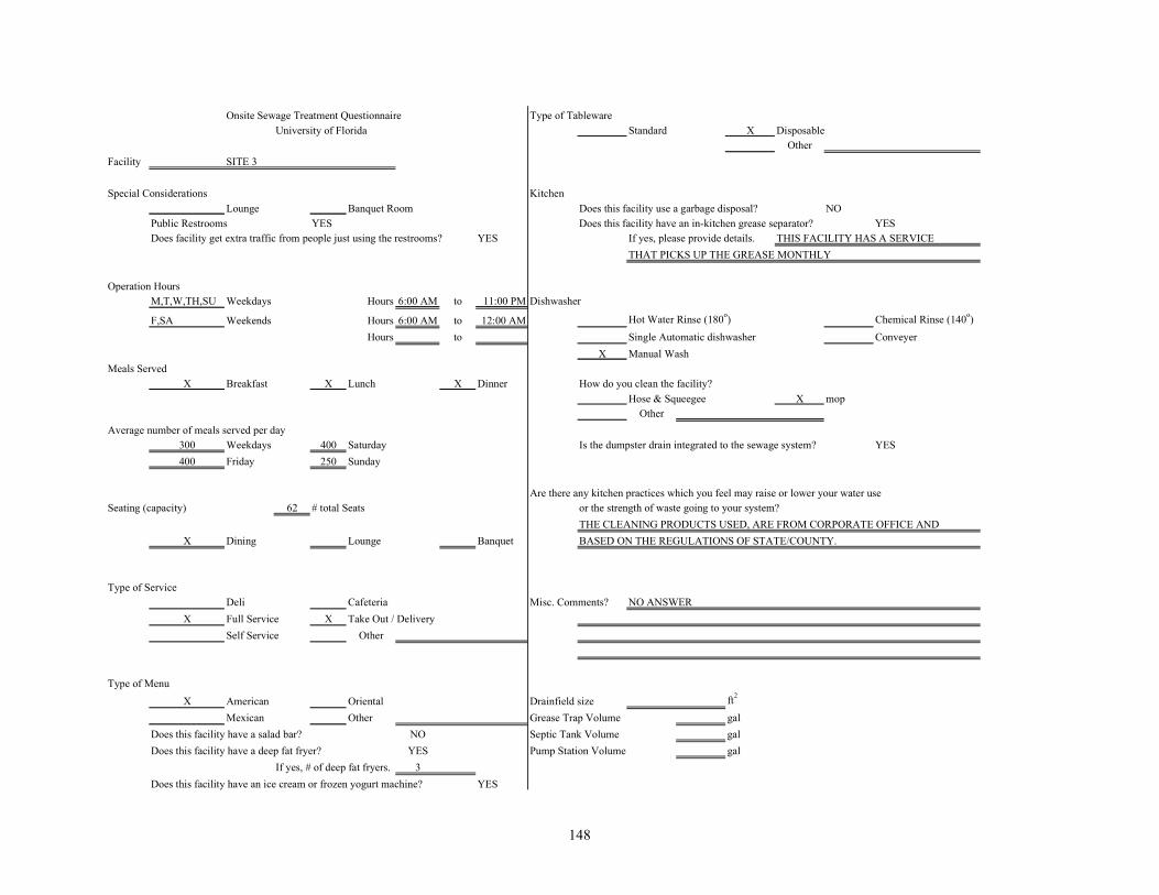
148

Onsite Sewage Treatment Questionnaire Type of Tableware University of Florida Standard X Disposable

OtherFacility SITE 3

Special Considerations Kitchen

Lounge Banquet Room Does this facility use a garbage disposal? NOPublic Restrooms YES Does this facility have an in-kitchen grease separator? YESDoes facility get extra traffic from people just using the restrooms? YES If yes, please provide details. THIS FACILITY HAS A SERVICE

THAT PICKS UP THE GREASE MONTHLY

Operation HoursM,T,W,TH,SU Weekdays Hours 6:00 AM to 11:00 PM Dishwasher

F,SA Weekends Hours 6:00 AM to 12:00 AM Hot Water Rinse (180o) Chemical Rinse (140o)Hours to Single Automatic dishwasher Conveyer

X Manual WashMeals Served

X Breakfast X Lunch X Dinner How do you clean the facility?Hose & Squeegee X mop

OtherAverage number of meals served per day

300 Weekdays 400 Saturday Is the dumpster drain integrated to the sewage system? YES400 Friday 250 Sunday

Are there any kitchen practices which you feel may raise or lower your water useSeating (capacity) 62 # total Seats or the strength of waste going to your system?

THE CLEANING PRODUCTS USED, ARE FROM CORPORATE OFFICE ANDX Dining Lounge Banquet BASED ON THE REGULATIONS OF STATE/COUNTY.

Type of ServiceDeli Cafeteria Misc. Comments? NO ANSWER

X Full Service X Take Out / DeliverySelf Service Other

Type of Menu

X American Oriental Drainfield size ft2

Mexican Other Grease Trap Volume galDoes this facility have a salad bar? NO Septic Tank Volume galDoes this facility have a deep fat fryer? YES Pump Station Volume gal

If yes, # of deep fat fryers. 3Does this facility have an ice cream or frozen yogurt machine? YES

149

Onsite Sewage Treatment Questionnaire Type of TablewareUniversity of Florida Standard X Disposable

OtherFacility SITE 4

Special Considerations KitchenLounge Banquet Room Does this facility use a garbage disposal? NO

Public Restrooms YES Does this facility have an in-kitchen grease separator? NODoes facility get extra traffic from people just using the restrooms? NO If yes, please provide details.

Operation HoursX Weekdays Hours 5:00 AM to 12:00 AM Dishwasher

X Weekends Hours 5:00 AM to 12:00 AM Hot Water Rinse (180o) Chemical Rinse (140o)Hours to Single Automatic dishwasher Conveyer

X Manual Wash Meals Served

X Breakfast X Lunch X Dinner How do you clean the facility?Hose & Squeegee X mop

OtherAverage number of meals served per day EXPRESS RESTAURANT

80 Weekdays 170 Saturday Is the dumpster drain integrated to the sewage system? NO160 Friday 160 Sunday

Are there any kitchen practices which you feel may raise or lower your water useSeating (capacity) 2 # total Seats or the strength of waste going to your system?

NO ANSWERDining X Lounge Banquet

Type of ServiceDeli Cafeteria Misc. Comments? NO ANSWERFull Service X Take Out / Delivery

X Self Service Other

Type of MenuAmerican Oriental

X Mexican Other Drainfield size ft2

Does this facility have a salad bar? NO Grease Trap Volume galDoes this facility have a deep fat fryer? NO Septic Tank Volume gal

If yes, # of deep fat fryers. Pump Station Volume galDoes this facility have an ice cream or frozen yogurt machine? NO

150

Onsite Sewage Treatment Questionnaire Type of Tableware University of Florida Standard X Disposable

OtherFacility SITE 5

Special Considerations KitchenLounge Banquet Room Does this facility use a garbage disposal? NO

Public Restrooms YES (2) Does this facility have an in-kitchen grease separator? NODoes facility get extra traffic from people just using the restrooms? NO If yes, please provide details.

Operation HoursX Weekdays Hours 5:00 AM to 12:00 AM Dishwasher

X Weekends Hours 5:00 AM to 12:00 AM Hot Water Rinse (180o) Chemical Rinse (140o)Hours to Single Automatic dishwasher Conveyer

X Manual Wash 3 COMPARTMENT SINKMeals Served

Breakfast X Lunch X Dinner How do you clean the facility?Hose & Squeegee X mop

OtherAverage number of meals served per day EXPRESS RESTAURANT

100 Weekdays Saturday Is the dumpster drain integrated to the sewage system? NOFriday Sunday

Are there any kitchen practices which you feel may raise or lower your water useSeating (capacity) 0 # total Seats or the strength of waste going to your system?

NO ANSWERDining Lounge Banquet

Type of ServiceDeli Cafeteria Misc. Comments? NO ANSWERFull Service X Take Out / Delivery

X Self Service Other

Type of MenuAmerican Oriental

X Mexican Other Drainfield size ft2

Does this facility have a salad bar? NO Grease Trap Volume galDoes this facility have a deep fat fryer? NO Septic Tank Volume gal

If yes, # of deep fat fryers. Pump Station Volume galDoes this facility have an ice cream or frozen yogurt machine? NO

151

Onsite Sewage Treatment Questionnaire Type of Tableware University of Florida Standard X Disposable

OtherFacility SITE 6

Special Considerations KitchenLounge Banquet Room Does this facility use a garbage disposal? NO

Public Restrooms YES Does this facility have an in-kitchen grease separator? NODoes facility get extra traffic from people just using the restrooms? YES If yes, please provide details.

Operation HoursX Weekdays Hours 5:30 AM to 11:00 PM Dishwasher

X Weekends Hours to Hot Water Rinse (180o) X Chemical Rinse (140o)Hours to Single Automatic dishwasher Conveyer

Manual WashMeals Served

X Breakfast X Lunch X Dinner How do you clean the facility?Hose & Squeegee X mop

OtherAverage number of meals served per day

728 Weekdays 972 Saturday Is the dumpster drain integrated to the sewage system? NO888 Friday 714 Sunday

Are there any kitchen practices which you feel may raise or lower your water useSeating (capacity) 94 # total Seats or the strength of waste going to your system?

NO ANSWERX Dining Lounge Banquet

Type of ServiceDeli Cafeteria Misc. Comments? NO ANSWER

X Full Service X e Out / DeliveryX Self Service Other

Type of Menu

X American Oriental Drainfield size ft2

Mexican Other Grease Trap Volume galDoes this facility have a salad bar? NO Septic Tank Volume galDoes this facility have a deep fat fryer? YES Pump Station Volume gal

If yes, # of deep fat fryers. 5Does this facility have an ice cream or frozen yogurt machine? YES

152

Onsite Sewage Treatment Questionnaire Type of Tableware University of Florida Standard X Disposable

OtherFacility SITE 7

Special Considerations KitchenLounge Banquet Room Does this facility use a garbage disposal? NO

Public Restrooms YES Does this facility have an in-kitchen grease separator? NODoes facility get extra traffic from people just using the restrooms? YES If yes, please provide details.

Operation HoursX Weekdays Hours 24 HRS to Dishwasher

X Weekends Hours 24 HRS to Hot Water Rinse (180o) Chemical Rinse (140o)Hours to Single Automatic dishwasher Conveyer

Manual WashMeals Served

X Breakfast X Lunch X Dinner How do you clean the facility?Hose & Squeegee X mop

OtherAverage number of meals served per day

Weekdays Saturday Is the dumpster drain integrated to the sewage system?Friday Sunday

Are there any kitchen practices which you feel may raise or lower your water useSeating (capacity) 20 # total Seats or the strength of waste going to your system?

NO ANSWERX Dining Lounge Banquet

Type of ServiceDeli Cafeteria Misc. Comments? NO ANSWER

X Full Service X Take Out / DeliverySelf Service Other

Type of MenuX American Oriental

X Mexican Other Drainfield size ft2

Does this facility have a salad bar? NO Grease Trap Volume galDoes this facility have a deep fat fryer? NO Septic Tank Volume gal

If yes, # of deep fat fryers. Pump Station Volume galDoes this facility have an ice cream or frozen yogurt machine? NO

153

Onsite Sewage Treatment Questionnaire Type of Tableware University of Florida X Standard Disposable

OtherFacility SITE 11

Special Considerations KitchenLounge Banquet Room Does this facility use a garbage disposal? NO

Public Restrooms YES Does this facility have an in-kitchen grease separator? NODoes facility get extra traffic from people just using the restrooms? NO If yes, please provide details.

Operation HoursX Weekdays Hours 11:00 AM to 10:00 PM Dishwasher

X Weekends Hours 6:00 AM to 10:00 PM X Hot Water Rinse (180o) Chemical Rinse (140o)Hours to Single Automatic dishwasher Conveyer

Manual WashMeals Served

X Breakfast X Lunch X Dinner How do you clean the facility?Hose & Squeegee mop

OtherAverage number of meals served per day

125 Weekdays 200 Saturday Is the dumpster drain integrated to the sewage system?200 Friday 200 Sunday

Are there any kitchen practices which you feel may raise or lower your water useSeating (capacity) 60 # total Seats or the strength of waste going to your system?

NO ANSWERX Dining Lounge Banquet

Type of Service Misc. Comments? GALLONS PER SEAT ARE NOT A RELIABLE SOURCE. ONSITEDeli Cafeteria SYSTEMS SHOULD BE REVIEWED AS TO SEVERAL TOPICS - SEATING

X Full Service Take Out / Delivery SHOULD BE CONSIDERED BUT IT SHOULD BO BE THE SOLE SOURCESelf Service Other FOR DETERMINATION OF SYSTEM SIZE. ACCORDING TO OUR SEATING

WE SHOULD HAVE A SYSTEM THAT HANDLES 17,000 GAL. OF SEWAGEA DAY, WE ONLY CONSUME 2,000-3,000 GAL OF WATER PER DAY -

Type of Menu TOTAL! MY ESTIMATES OF SEWAGE FLOW WOULD BE ABOUT 50%X American Oriental OF THAT FIGURE. USING THAT, WE SHOULD BE ABLE TO INCREASE

Mexican Other OUR SEATING TO 10 TIMES WHAT WE ARE ALLOWED.

Does this facility have a salad bar? YES Drainfield size ft2

Does this facility have a deep fat fryer? YES Grease Trap Volume galIf yes, # of deep fat fryers. Septic Tank Volume gal

Does this facility have an ice cream or frozen yogurt machine? NO Pump Station Volume gal

154

Onsite Sewage Treatment Questionnaire Type of Tableware University of Florida X Standard Disposable

OtherFacility SITE 12

Special Considerations KitchenLounge Banquet Room Does this facility use a garbage disposal? NO

Public Restrooms YES Does this facility have an in-kitchen grease separator? YESDoes facility get extra traffic from people just using the restrooms? YES If yes, please provide details.

Operation HoursX Weekdays Hours 6:00 AM to 9:00 PM Dishwasher

X Weekends Hours 6:00 AM to 10:00 PM X Hot Water Rinse (180o) Chemical Rinse (140o)

Hours to Single Automatic dishwasher ConveyerManual Wash

Meals ServedX Breakfast X Lunch X Dinner How do you clean the facility?

Hose & Squeegee mopOther

Average number of meals served per day200 Weekdays 500 Saturday Is the dumpster drain integrated to the sewage system?500 Friday 430 Sunday

Are there any kitchen practices which you feel may raise or lower your water useSeating (capacity) 85 # total Seats or the strength of waste going to your system?

NO ANSWERX Dining Lounge Banquet

Type of ServiceDeli Cafeteria Misc. Comments? NO ANSWER

X Full Service X Take Out / DeliverySelf Service Other

Type of MenuX American Oriental

Mexican Other Drainfield size ft2

Does this facility have a salad bar? NO Grease Trap Volume galDoes this facility have a deep fat fryer? YES Septic Tank Volume gal

If yes, # of deep fat fryers. Pump Station Volume galDoes this facility have an ice cream or frozen yogurt machine? NO

155

Onsite Sewage Treatment Questionnaire Type of Tableware University of Florida Standard X Disposable

OtherFacility SITE 13

Special Considerations KitchenLounge Banquet Room Does this facility use a garbage disposal? NO

Public Restrooms YES Does this facility have an in-kitchen grease separator? NODoes facility get extra traffic from people just using the restrooms? YES If yes, please provide details.

Operation HoursX Weekdays Hours 24 HRS to Dishwasher

X Weekends Hours 24 HRS to Hot Water Rinse (180o) Chemical Rinse (140o)Hours to X Single Automatic dishwasher Conveyer

Manual WashMeals Served

X Breakfast X Lunch X Dinner How do you clean the facility?Hose & Squeegee X mop

OtherAverage number of meals served per day

500 Weekdays 1,000 Saturday Is the dumpster drain integrated to the sewage system?1,000 Friday 700 Sunday

Are there any kitchen practices which you feel may raise or lower your water useSeating (capacity) 60 # total Seats or the strength of waste going to your system?

NO ANSWERX Dining Lounge Banquet

Type of ServiceDeli Cafeteria Misc. Comments? NO ANSWER

X Full Service X Take Out / DeliverySelf Service Other

Type of MenuX American Oriental

Mexican OtherDoes this facility have a salad bar? NO

Does this facility have a deep fat fryer? YES Drainfield size ft2

If yes, # of deep fat fryers. 4 Grease Trap Volume galDoes this facility have an ice cream or frozen yogurt machine? YES Septic Tank Volume gal

Pump Station Volume gal

156

Onsite Sewage Treatment Questionnaire Type of Tableware University of Florida X Standard Disposable

OtherFacility SITE 14

Special Considerations KitchenLounge Banquet Room Does this facility use a garbage disposal? NO

Public Restrooms YES (2) Does this facility have an in-kitchen grease separator? NODoes facility get extra traffic from people just using the restrooms? YES If yes, please provide details. THIS FACILITY HAS A COMPANY

THAT PICKS UP THE GREASE MONTHLY

Operation HoursX Weekdays Hours 6:00 AM to 10:00 PM Dishwasher

X Weekends SAT Hours 6:00 AM to 2:00 PM X Hot Water Rinse (180o) Chemical Rinse (140o)SUN Hours 6:00 AM to 4:00 PM Single Automatic dishwasher Conveyer

Manual WashMeals Served

X Breakfast X Lunch X Dinner How do you clean the facility?Hose & Squeegee X mop

OtherAverage number of meals served per day

200 Weekdays 350 Saturday Is the dumpster drain integrated to the sewage system? NO300 Friday 300 Sunday

Are there any kitchen practices which you feel may raise or lower your water useSeating (capacity) 50 # total Seats or the strength of waste going to your system?

NO ANSWERX Dining Lounge Banquet

Type of ServiceDeli Cafeteria Misc. Comments? NO ANSWER

X Full Service Take Out / DeliverySelf Service Other

Type of Menu Drainfield size ft2

X American Oriental Grease Trap Volume galMexican Other Septic Tank Volume gal

Does this facility have a salad bar? YES Pump Station Volume galDoes this facility have a deep fat fryer? YES

If yes, # of deep fat fryers. 1Does this facility have an ice cream or frozen yogurt machine? NO

157

Onsite Sewage Treatment Questionnaire

University of Florida Type of TablewareX Standard Disposable

Facility SITE 15 Other

Special ConsiderationsLounge X Banquet Room Kitchen

Public Restrooms YES (2) Does this facility use a garbage disposal? NODoes facility get extra traffic from people just using the restrooms? NO Does this facility have an in-kitchen grease separator? NO

If yes, please provide details.

Operation HoursM,T,W Hours 6:30 AM to 3:00 PMTH,F,S Hours 6:00 AM to 10:00 PM Dishwasher

SUN Hours 6:30 AM to 9:00 PM X Hot Water Rinse (180o) Chemical Rinse (140o) Single Automatic dishwasher Conveyer

Manual WashMeals Served

X Breakfast X Lunch X Dinner How do you clean the facility?X Hose & Squeegee X mop

OtherAverage number of meals served per day

275 Weekdays 450 Saturday Is the dumpster drain integrated to the sewage system? NO400 Friday 450 Sunday

Are there any kitchen practices which you feel may raise or lower your water useSeating (capacity) 125 # total Seats or the strength of waste going to your system?

NO ANSWERX Dining Lounge Banquet

Type of Service Misc. Comments? NO ANSWERDeli Cafeteria

X Full Service X Take Out / DeliverySelf Service Other

Type of Menu Drainfield size ft2

American Oriental Grease Trap Volume gal Mexican X Other SEAFOOD Septic Tank Volume gal

Does this facility have a salad bar? YES Pump Station Volume galDoes this facility have a deep fat fryer? YES

If yes, # of deep fat fryers. 3 2 GREASE TRAPSDoes this facility have an ice cream or frozen yogurt machine? NO 3 DRAINFIELDS EACH 2000 SQ FT

LIFT STATATION (1,800 OR 2,500 ?) GAL

158

APPENDIX E RESTAURANT SITE PLANS

159

o 50' 100'

I I

lNroRllATION _. -~-- --,,,. ","-y \WM -

--.= SITE #02

,- "", -- 2- Sl THIAP

)

I I ,

I' _~ • ••• ", ~ HUe """" sr

ut.l"VERSITY or f'lDRIDA

= rnH ... 02-snE PAGE

J..",,-.1

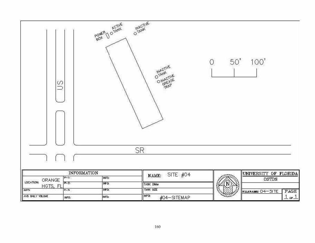
160

o 50' 100'

LI~I_I

SR In

SITE #04-L.OCA """ OR A N GE

161

"" ." ,J ,

D

DD 0 0 0 0

0 0 0 0

"

"'CO "". " ~

lNroRllATION RillE: SITE ,05 UNIVERSITY OF FLORIDA

,""",.".. " - O~ ~,~

SPRINGS fAIt< OOJ, - • • mJ!X ...... , 06 '" PAGE - w, 00 SlTEMAP , . ,

162

ESTABLISHMENT

° 0,---_____ ----,

° 45' DRAINFIELD

47'

163

PARKING

·oc ""tlI<, ,ct" SEPT<: T>N.S 0 '«EllS, ........ S· I 0 0 0 I

P'lH' . ,,"' 1,/:' ", 11 0 VAC

" ~o Hz 2' 0,

DD N.u!E: SITE 1/10

DRY RETENTION POND

o I

........ ""'"' 1/~ "P 11 ' VN:.

" '" H, " ,

50' 100'

I

164

1 050 ~al GREASE TRAP

2800 ga l SEPTlC TAN K

1O~O gal LIFT STATION

DRAINFIELD: :::ED-SYSTEM

o

o

ILm E: SITE #11

165

I

r LIFT " 80X[ I

LIFT ~

0 ~

GREASE TRAPO

20' 40' ALARM D 0 0 x I I PROPANE I 0

? 'i' rR()~ T / ~A~HOLE TO T/ GREASE

I

lNroRYATION SITE #12

(I UNIVERSITY OF FlllRIDA HAllE:

O~ " -~- TAIt( OOJ,

• ron ...... ' 12 SITE PAGE - • • , . , ", .E SITE~AP AI<) ","-y ""-'-'" -

166

o e < , w Z; ~ , ~

~

~

~

o w m " o

, ~ • w

l ro 0

"" '" '" z '" g !:::- ~ :ii 0 ~ m ",>->-~ "-12-z"o~ g",(f) -::0 " '" "' ~ '" w >-~ >- "- Q

:<:",,-,22,,- ZD Z -«>->-oo:J «:"'w "" "- '" ~ ~ ::i! l;j t.I ~ <:t g, 0 e < W (f) W o "'0 WC<-'wwO(j ""0 0zz,,

UUUUU , , • , ,

, , ,

, t t " t

,

, 5

, ~ ~ ~ ~ • , " " " "

, tttttt

ttttttt

, f

L=,,1 D

t t t t

t t t t

I i o

+ + t + , , , , , , , , , ,

•

,

o z , "' Ii

~ ~~ co

~

0-1 ~ , "-I "T""

" " • !

(j

+

'" ~ w

~

I

I

iii

; !

n Z

~ w z U

1

I

" <

~ o

I~ I

!

167

o 50' 100'

LI~I_I

In SITE #15

L.OCA """ OR A N G E