final data evaluation and summary report

Port Gardner Bay Regional Background Sediment Characterization

Everett, WA

Final Data Evaluation and Summary Report December 31, 2014 Publication no. 14-09-339

Publication and Contact Information

This report is available on the Department of Ecology’s website at www.ecy.wa.gov/biblio/1409339.html For more information contact: Toxics Cleanup Program P.O. Box 47600 Olympia, WA 98504-7600

Phone: 800-826-7716

Washington State Department of Ecology - www.ecy.wa.gov

o Headquarters, Olympia 360-407-6000

o Northwest Regional Office, Bellevue 425-649-7000

o Southwest Regional Office, Olympia 360-407-6300

o Central Regional Office, Yakima 509-575-2490

o Eastern Regional Office, Spokane 509-329-3400 To request ADA accommodation including materials in a format for the visually impaired, call the Toxics Cleanup Program at 800-826-7716. Persons with impaired hearing may call Washington Relay Service at 711. Persons with speech disability may call TTY at 877-833-6341.

Port Gardner Bay Regional Background Sediment

Characterization

Final Data Evaluation and Summary Report

Prepared by

Washington State Department of Ecology Toxics Cleanup Program

Olympia, WA

115 2nd Ave N

Suite 100 Edmonds, WA 98020

TerraStat Consulting Group

Avocet Consulting

i

Table of Contents

Page

Appendices ..................................................................................................................... i List of Figures .............................................................................................................. iii List of Tables ............................................................................................................... iii List of Acronyms ......................................................................................................... iv

1.0 Introduction ...........................................................................................................1 1.1. Regional Background Definition .....................................................................1 1.2. Stakeholder Discussions ..................................................................................2 1.3. Phase II Area of Interest ..................................................................................3

2.0 Sampling Methods and Analysis ...........................................................................5 2.1. Station Positioning and Navigation .................................................................5 2.2. Surface Sediment Grabs ...................................................................................6 2.3. Sample Storage, Delivery, and Chain of Custody ...........................................6

2.3.1. Laboratory Analysis .................................................................................7

3.0 Data Validation ......................................................................................................9

4.0 Data Results .........................................................................................................11 4.1. Calculation of Toxicity Equivalents ..............................................................11 4.2. Summary of Qualified Results .......................................................................12 4.3. Summary and Spatial Distribution of Results ................................................13

4.3.1. Conventional Parameters .......................................................................14 4.3.2. Metals .....................................................................................................14 4.3.3. Organics .................................................................................................14 4.3.4. Chemical Distribution Summary ...........................................................15

5.0 Data Analysis .......................................................................................................16 5.1. Natural Background for Port Gardner Bay Bay .............................................16 5.2. Potential Analysis of Secondary Samples ......................................................16 5.3. Outlier Analysis .............................................................................................17 5.4. Calculation of Port Gardner Bay 90/90 UTLs and Regional Background Values 19

6.0 References ...........................................................................................................21

Appendices (A – D, F, and G available at: www.ecy.wa.gov/biblio/1409339.html)

Appendix A. Field Sampling Notes Appendix B. Surface Sediment Grab Logbook Appendix C. Sample Container Logbook Appendix D. Chain of Custody Forms Appendix E. Data Tables Appendix F. Analytical Laboratory Reports Appendix G. EcoChem Data Validation Report Appendix H. Univariate and Multivariate Investigations of the Port Gardner Bay Data Set

iii

List of Figures and Tables

List of Figures Figure 1. Phase I and Phase II Study Areas in Port Gardner Bay.

Figure 2. Sample Locations Included in the Phase II Study Area.

Figure 3. Summary of Undetected and Qualified Results.

Figure 4. Percent Total Organic Carbon and Grain Size Distributions Throughout the Port Gardner Bay Area of Interest.

Figure 5. Arsenic Concentrations Throughout the Port Gardner Bay Area of Interest.

Figure 6. Cadmium Concentrations Throughout the Port Gardner Bay Area of Interest.

Figure 7. Mercury Concentrations Throughout the Port Gardner Bay Area of Interest.

Figure 8. Carcinogenic Polycyclic Aromatic Hydrocarbons (cPAH) TEQ Concentrations (KM) Throughout the Port Gardner Bay Area of Interest.

Figure 9. Dioxin/Furan Congener TEQ Concentrations (KM) Throughout the Port Gardner Bay Area of Interest.

Figure 10. Polychlorinated Biphenyl (PCB) TEQ Concentrations (KM) Throughout the Port Gardner Bay Area of Interest.

Figure 11. Decision Process for the Evaluation of Secondary Samples.

List of Tables Table 1. Location depths, actual coordinates, distance from target, and percent fines for

Port Gardner Bay Regional Background sampling.

Table 2. Collected sediment samples, target analytes, and analytical methods.

Table 3. Target analytes, methods, and practical quantitation limits.

Table 4. Summary statistics and correlation to percent fines and total organic carbon (TOC) for target contaminants.

Table 5. Statistical summary of Port Gardner Bay Phase II data.

Table 6. Calculated 90/90 upper tolerance limits (UTL) for Port Gardner Bay and Bold Plus natural background data sets.

iv

List of Acronyms AOI Area of Interest ARI Analytical Resources Inc. Axys Axys Analytical Ltd. CoC chemical of concern CRM certified reference material cPAH carcinogenic polycyclic aromatic hydrocarbon CSL Cleanup Screening Level DGPS differential global positioning system DMMP Dredged Material Management Program DQO data quality objectives Ecology Washington State Department of Ecology EMPC estimated maximum potential concentration EPA U.S. Environmental Protection Agency KM Kaplan-Meier MCD minimum covariance determinant MDL method detection limit MLLW mean lower low water MTCA Model Toxics Control Act NAD83 1983 North American Datum OCDF octachlorodibenzodioxin PCA principal component analysis PCB polychlorinated biphenyl Phase I regional background samples collected in 2013 Phase II regional background samples collected in 2014 PQL practical quantitation limit PSEP Puget Sound Estuary Program PSRM Puget Sound reference material QA/QC Quality Assurance/Quality Control RPD relative percent difference RSD relative standard deviation SAP Sampling and Analysis Plan SCO Sediment Cleanup Objective SCUM II Sediment Cleanup User’s Manual II SDL sample specific detection limit SIM select ion monitoring SMS Sediment Management Standards SRM standard reference material TCDD 2,3,7,8-Tetrachlorodibenzodioxin TEC toxic equivalent concentration

v

TEF toxic equivalent factor TEQ toxic equivalent quotient TOC total organic carbon UCL upper confidence limit UTL upper tolerance limit WAC Washington Administrative Code WHO World Health Organization

December 31, 2014 1 Final Data Evaluation and Summary Report

1.0 Introduction

Port Gardner Bay is one of several embayments identified for focused sediment investigation, cleanup, and source control under the Washington State Department of Ecology (Ecology) Toxics Cleanup Program’s Puget Sound Initiative. In early 2013, Ecology revised its Sediment Management Standards (SMS) to establish a new framework for identification and cleanup of contaminated sediment sites (Washington Administrative Code [WAC] 173-204). A key component of this framework was the concept of regional background sediment concentrations, which could potentially serve as the Cleanup Screening Level (CSL) for sediment sites.

Initial efforts were made in 2013 to collect samples representative of regional background from Port Gardner Bay (Phase I). However, as Ecology’s approach to evaluating regional background evolved due to internal review, tribal and stakeholder review, and public comment, portions of this data set were determined to be unrepresentative of regional background and not consistent with the intent of the SMS rule (WAC 173-204-505(16) and 173-204-560(5)). For example, samples collected from the Snohomish River delta were determined to be more representative of natural background (WAC 173-204-505(11)). As a result, Ecology identified new areas representative of regional background which included adding areas closer to the shoreline and removing Phase I areas influenced by the Snohomish River Delta for supplemental sampling. This supplemental sampling occurred in 2014 (Phase II). This report presents the combined sampling data from Phases I and II for calculation of regional background for Port Gardner Bay. Lessons learned during sampling and evaluation of these results will serve as one example to inform sample location placement and study design for future regional background characterization work in other areas of the state.

1.1. Regional Background Definition

For a number of bioaccumulative chemicals, risk-based values protective of human health and upper trophic levels fall below natural background concentrations, as defined in the SMS (WAC 173-204-505(11)). Sediments are a sink for chemicals from potentially hundreds of sources, including a mix of permitted and unpermitted stormwater, atmospheric deposition, and historical releases from industrial activities. In urban embayments with developed shorelines, chemical concentrations in sediment are frequently higher than natural background concentrations.

The 2013 SMS rule revisions retained the two-tiered framework used to establish sediment cleanup levels, but now incorporates natural background (as the potential Sediment Cleanup Objective (SCO)) and a new term and concept, regional background as the potential CSL. The SMS rule includes a definition for regional background (WAC 173-204-505(16)) and parameters for establishing regional background (WAC 173-204-560(5)):


“Regional Background” means the concentration of a contaminant within a department-defined geographic area that is primarily attributable to diffuse sources, such as atmospheric deposition or storm water, not attributable to a specific source or release.

The SMS rule is intended to provide flexibility to establish regional background on a case-by-case basis and does not specifically prescribe how regional background should be established. The approach and methods contained in the Phase I and Phase II Port Gardner Bay Regional Background Sampling and Analysis Plans (SAP; Ecology 2013a, Ecology 2014) were developed by Ecology to establish regional background concentrations for selected analytes: arsenic, cadmium, mercury, carcinogenic polycyclic hydrocarbons (cPAHs), dioxins/furans, and polychlorinated biphenyls (PCBs) in Port Gardner Bay. This study serves as one example of how regional background concentrations can be established in a particular Ecology-defined geographic area. Ecology’s approach to establishing regional background has evolved over time through working on initial bays and after receiving comments from stakeholders and tribes, as described below.

1.2. Stakeholder Discussions

In 2013, Ecology received a number of comments from stakeholders and tribes on the Phase I Port Gardner Bay Regional Background SAP (Ecology 2013a) and the North Olympic Peninsula Regional Background SAP (Ecology 2013c), some of which were incorporated into the final SAPs. Many stakeholders requested that for future regional background characterizations, they would like to work with Ecology before SAPs were drafted and submitted for public comment. In response, Ecology engaged stakeholders earlier in the process for the initial discussions regarding establishing regional background for Elliott Bay and/or the Lower Duwamish River and Bellingham Bay.

The early involvement for Elliott Bay/Lower Duwamish River included conducting a series of interviews with key regional stakeholders in June 2013 to prepare for a September 2013 technical workshop to 1) discuss whether to establish regional background in Elliott Bay and/or the Lower Duwamish River, 2) share information and data, including stakeholder and Ecology presentations, and 3) collaboratively work on the sampling design, which included discussion of alternative sampling approaches for both areas. In addition, Ecology received a number of follow up comment letters after this technical workshop.

Subsequently, the Phase I Port Gardner Bay data package containing the data, graphs, figures, and limited data interpretation was provided to stakeholders and tribes on August 5, 2013 for review and comment. Ecology received a number of comments on the Port Gardner Bay data package, as well as concurrent discussions related to regional background sampling in the North Olympic Peninsula.


Based on all of the above comments and discussions, Ecology determined that some modifications to the Phase I Port Gardner Bay sampling design were appropriate. These changes were incorporated into the Phase II Port Gardner Bay SAP (Ecology 2014) and the revised approach will be updated in the Sediment Cleanup Users Manual II guidance (SCUM II, Ecology 2013b).

The following major modifications were incorporated into the Phase II SAP for Port Gardner Bay:

Rationale and Conceptual Bay Model. A discussion of the selected analytes, existing information used to develop the sampling area of interest, and the rationale for the selected sampling method(s). These choices were based on a conceptual bay model developed for Port Gardner Bay and key features of the bay that influenced these decisions. These include known sites and sources, existing chemistry data, existing modeling information, hydrodynamic information, bathymetry, etc.

Sampling Area. The area in which the Phase II sediment samples were collected was modified to be more consistent with the SMS definition of regional background (WAC 173-204-505(16)). The Phase I areas more representative of natural background were excluded, while new areas representative of regional background were added. This entailed sampling closer to the shoreline, sources, and sites, while remaining outside areas of direct influence from known or suspected sources for the regional background CoCs (WAC 173-204-560(5)(d)). A default distance from these areas was no longer used. Instead, bay-specific information was used, where available, to determine areas associated with the depositional zones of outfalls or other point sources and areas directly affected by sites. Accordingly, the Phase II SAP included collection of samples in nearshore areas that were not sampled in Phase I (Ecology 2013a, Ecology 2014). This was done in such a way that the data were able to be statistically combined with the Phase I samples collected in 2013.

This new approach and lessons learned have been applied to the SAP design for Bellingham Bay, in addition to bay-specific modifications.

1.3. Phase II Area of Interest

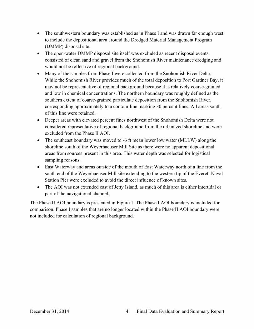
Regional background concentrations for Port Gardner Bay were determined based on data from samples collected within the Phase II area of interest (AOI; Figure 1). Portions of this AOI boundary were consistent with the Phase I SAP, while the northern and eastern boundaries were modified as discussed above. Based on the conceptual bay model, the Phase II AOI was defined as follows:


The southwestern boundary was established as in Phase I and was drawn far enough west to include the depositional area around the Dredged Material Management Program (DMMP) disposal site.

The open-water DMMP disposal site itself was excluded as recent disposal events consisted of clean sand and gravel from the Snohomish River maintenance dredging and would not be reflective of regional background.

Many of the samples from Phase I were collected from the Snohomish River Delta. While the Snohomish River provides much of the total deposition to Port Gardner Bay, it may not be representative of regional background because it is relatively coarse-grained and low in chemical concentrations. The northern boundary was roughly defined as the southern extent of coarse-grained particulate deposition from the Snohomish River, corresponding approximately to a contour line marking 30 percent fines. All areas south of this line were retained.

Deeper areas with elevated percent fines northwest of the Snohomish Delta were not considered representative of regional background from the urbanized shoreline and were excluded from the Phase II AOI.

The southeast boundary was moved to -6 ft mean lower low water (MLLW) along the shoreline south of the Weyerhaeuser Mill Site as there were no apparent depositional areas from sources present in this area. This water depth was selected for logistical sampling reasons.

East Waterway and areas outside of the mouth of East Waterway north of a line from the south end of the Weyerhaeuser Mill site extending to the western tip of the Everett Naval Station Pier were excluded to avoid the direct influence of known sites.

The AOI was not extended east of Jetty Island, as much of this area is either intertidal or part of the navigational channel.

The Phase II AOI boundary is presented in Figure 1. The Phase I AOI boundary is included for comparison. Phase I samples that are no longer located within the Phase II AOI boundary were not included for calculation of regional background.


2.0 Sampling Methods and Analysis

Phase I sediment sampling was conducted from March 26 through March 29, 2013. Phase II sampling was conducted April 22 and 23, 2014. For both phases, sampling was conducted within the respective AOI shown in Figure 1. The target locations were mapped within each AOI such that no samples would be collected within 500 meters of each other (Ecology 2013a, Ecology 2014).

Sediment collection within the AOI consisted of two types of samples, baseline and secondary. The same volume of sediment was collected for both sample types following the same collection methodologies. The difference between the sample types was that baseline samples were submitted for analysis of the full suite of chemicals, while secondary samples were initially analyzed for mercury and total sulfides due to short holding times. Secondary samples were also analyzed for grain size to better characterize the physical characteristics of the AOI and to aid in the selection of secondary samples for potential analysis. The remainder of the sediment from the secondary samples was archived for potential future analysis. Sample counts for each phase are as follows:

25 baseline samples and 25 secondary samples were collected as part of Phase I. 15 of these sample locations were located within the Phase II AOI and were incorporated into the Phase II data set.

12 new baseline and 3 new secondary samples were collected as part of Phase II.

A total of 27 baseline samples and 3 secondary samples were integrated into the Phase II dataset. The target sampling locations were randomly placed throughout the AOI to ensure a minimum distance of 500 meters between sampling locations.

2.1. Station Positioning and Navigation

The R/V Kittiwake was used for the surface sediment grabs for both phases of sampling. A differential global positioning system (DGPS) was used aboard the R/V Kittiwake for station positioning. The baseline and secondary sampling location target coordinates were provided in advance and programmed into the R/V Kittiwake’s navigation system. Upon sampling device deployment, the actual position was recorded once the device reached the seafloor and the winch cable was in a vertical position. Latitude and longitude station coordinates were recorded in degrees decimal minutes using the 1983 North American Datum (NAD83). Water depths were measured using the winch meter wheel and verified by the ship’s fathometer. Table 1 provides the actual coordinates, water depths, and distance between the target and actual locations for the baseline and secondary sample locations, respectively. Figure 2 shows the actual locations for the baseline and secondary samples, respectively, and notes whether the samples were collected as part of Phase I or II.


There were two instances where a grab could not be collected at the target location. The first two grabs at PG-12-S were mostly washed out and contained rocks and shell hash. A successful grab was collected on the third attempt approximately 300 meters south of the target location (Table 1). Multiple efforts were made to collect a grab in the vicinity of PG-56-S. However, the grab could not close due to the presence of large woody debris and cobble. A successful grab was collected 293 meters north of the target (Table 1).

2.2. Surface Sediment Grabs

Surface sediment grabs were collected at 30 locations; 15 as part of Phase I and 15 as part of Phase II. All samples were collected using a stainless steel van Veen grab sampler deployed as either a dual or single bucket (0.1 m2 per bucket). Sampling followed the step wise procedure outlined in the SAP (Ecology 2013a, Ecology 2014). Notes related to sampling activities are presented in Appendix A. A brief summary of field sampling methods is provided below.

Established deployment and recovery procedures for the grab sampling gear, described by the Puget Sound Estuary Program (PSEP), were followed to ensure recovery of the best possible samples and minimize risks to personnel and equipment (PSEP 1997). Once a grab sample was retrieved, the overlying water was carefully siphoned off one side of the sampler. If the sample was judged to be acceptable according to PSEP specifications, the penetration depth was measured with a decontaminated stainless steel ruler, and sample quality, color, odor, and texture were described in the sample log. Scanned copies of the surface sediment grab logbook are presented in Appendix B.

The target depth for surface sediment collection was 10 cm. Only two samples, PG-01-S and PG-53-S, with penetration depths of 9.5 cm did not meet the target depth. There was slight over penetration in PG-44-S, however very little surface sediment was disturbed and the grab was deemed acceptable.

Percent fines were determined at each location by rinsing 40 ml of sediment through a 63.5 µ sieve until the water was clear. Percent fines are equal to 40 minus the volume of remaining sediment divided by 40. The amount of sediment retained on the sieve was recorded in the surface sediment grab logbook (Appendix B).

2.3. Sample Storage, Delivery, and Chain of Custody

After filling the jars with homogenized aliquots of sediment, all samples were labeled and the lids were wrapped with electrical tape to seal the jars and prevent leakage. Each label was marked with a jar tag number for tracking purposes. Sample identification and jar tag numbers were recorded in the sample container logbook (Appendix C).


After labeling, all samples were stored in insulated coolers and preserved by cooling to a temperature of 4ºC.

Samples were picked up by or delivered to Analytical Resources Incorporated (ARI; Tukwila, WA), while samples were shipped to Axys Analytical (Sidney, BC). Archived sediment from the Phase I secondary samples were stored at the Environ biological laboratory in Port Gamble, WA and disposed of after one year. Select Phase I secondary samples were removed from archival and submitted for analysis of the full suite of chemicals (Section 2.3.1). Archived sediment from the Phase II secondary samples were submitted to ARI. All archived samples were frozen at -18°C. The Chain of Custody forms for all samples are presented in Appendix D.

2.3.1. Laboratory Analysis

Samples were submitted to laboratories subcontracted by NewFields to conduct the chemical analyses. Axys analyzed the samples for dioxin/furan and PCB congeners. ARI analyzed samples for the sediment conventionals (total organic carbon [TOC], total solids, total volatile solids [TVS], grain size, and total sulfides), arsenic, cadmium, mercury, and cPAHs. Table 2 presents a list of all samples collected as part of the Phase II effort and includes the relevant analytical methods.

Within Table 2, samples PG-27, PG-28, PG-31, and PG-34 were secondary samples collected in 2013 as part of Phase I but analyzed separately from the remainder of the Phase I and II samples. These samples were analyzed for PCB congeners in 2013 due to the need for a larger sample size (Section 5.2). Archived sediment from these locations was submitted to ARI for analysis of arsenic, cadmium, and cPAHs. Archived sediment was submitted to Axys Analytical for analysis of dioxin/furan congeners. All archived samples were submitted in March 2014 and were received by the laboratories and extracted prior to the expiration of the one year holding time.

Additional samples collected for quality assurance/quality control (QA/QC) purposes are listed in Table 2. Full duplicates and triplicates were collected at locations PG-10 and PG-65. Rinsate blanks and equipment rinsate samples for metals and cPAHs were also collected as part of field sampling for both phases. Further details relating to chemical analysis can be found in the SAPs (Ecology 2013a, Ecology 2014).

Because of expected low concentrations, the data quality objectives (DQOs) used in this study were more stringent than those required for most sediment characterizations. As a result, the target practical quantitation limits (PQLs) for analysis were lower than most standard methods could provide. The PQLs for the analytes are listed in Table 3. This table includes the PQLs for the dioxin-like PCB congeners. The PQLs for the non-listed PCB congeners were all 0.4 ng/kg. The PQLs for the conventional parameters and the full list of PCB congeners can be found in the SAP (Ecology 2013a, Ecology 2014).

All non-detect sample results for cPAHs were reported to the method detection limit (MDL) and detected results less than the target PQL were “J” qualified. All non-detect results for metals


were reported at the PQL. Metals data are not qualified below the PQL. Non-detect results for dioxin/furan and PCB congeners were reported at the sample specific detection limit (SDL). All detected congener results less than the PQL were “J” qualified.

Laboratories do not provide PQL values for toxicity equivalent (TEQ) concentrations. Instead, these values were calculated for cPAHs, dioxin/furan congeners, and PCB congeners using the toxicity equivalency factors (TEF) from SCUM II for determining TEQ values (Ecology, 2013b) and the individual compound or congener specific PQLs in Table 3. The Ecology guidance for determining TEQs uses the dioxin/furan TEF values updated by the World Health Organization (WHO) in 2005 (Van den Berg et al. 2006). The resulting PQL for cPAHs was 0.76 µg TEQ/kg. The PQLs for dioxin/furan and PCB congeners were 2.3 and 0.052 ng TEQ/kg, respectively.

Cadmium was analyzed by Environmental Protection Agency (EPA) Method 200.8, which dictates results be reported at two significant figures for concentrations under 10 mg/kg. To meet this criterion, ARI reported cadmium concentrations below 10 mg/kg to one decimal place. However, this reporting system means concentrations less than 1 mg/kg contain only one significant figure. Many of the cadmium concentrations reported for this background study were below 1 mg/kg, meaning results are listed at one significant figure in the data packages in Appendix F. ARI was able to provide the metals analysis sheets that contain additional decimal places for cadmium. Cadmium concentrations measured to two decimal places were taken from these sheets and used in the final data tables (Appendix E) and the reporting and statistical analysis discussions.


3.0 Data Validation

A QA2 (EPA Stage 3/4) chemistry data review was conducted by EcoChem, Inc. (Seattle, WA) who examined the complete analytical process from calculation of instrument and method detection limits, PQLs, final dilution volumes, sample size, and wet-to-dry ratios to quantification of calibration compounds and all analytes detected in blanks and environmental samples (PTI 1989a; PTI 1989b; USEPA 2009). The intent of the independent data validation was to ensure that the investigation data results are defensible and usable for their intended purpose. This section provides a brief summary of the data validation reports for the Phase I and II analysis. Two validation reports were completed for Phase I including one for the initial round of analysis and another for the PCB congeners analyzed from the secondary samples. The full validation reports are provided in Appendix G.

When necessary, EcoChem applied the following data qualifiers to the chemical results:

U: The analyte was analyzed for, but was not detected above the reported sample quantitation limit.

UJ: The analyte was not detected above the reported sample quantitation limit. However, the reported quantitation limit is approximate and may or may not represent the actual limit of quantitation necessary to accurately and precisely measure the analyte.

J: The analyte was positively identified. The associated numerical value is the approximate concentration of the analyte. “J” qualifiers were assigned by the laboratories for results less than the PQL and greater than the MDL, or by EcoChem for results that failed to meet study specific QA/QC criteria.

DNR: Do not report. A more appropriate result is reported from another analysis or dilution.

The use of the DNR qualifier was limited to selecting the appropriate results for 2,3,7,8-TCDF, as results were reported for analysis on two separate columns. The remainder of the data was usable. Reason codes for applying the “U,” “UJ,” and “J” qualifiers and the definition for these codes are given in the validation reports (Appendix G).

Several qualifiers given by Axys were reclassified by EcoChem. Axys gave a “B” qualifier to all results where the analyte was detected in the method blank. EcoChem established an action level of five times the blank concentration. If a sample result was above that, the “B” qualifier was removed. If the result was below the action level, the result was qualified as un-detected (“U”).

The laboratory assigned “K” qualifiers to dioxin/furan and PCB congener data. This qualifier implied that a peak was detected, but did not meet identification criteria. These data were considered estimated maximum possible concentrations (EMPC). All EMPC results were given a “U” qualifier by EcoChem, but remained at the reported concentration which represented an elevated PQL for that congener.


Project specific QA/QC measures were employed during sample collection and analysis to ensure the precision, accuracy, and reproducibility of the results. This included field QA/QC samples such as equipment rinsate blanks, rinsate blanks, and field duplicates and triplicates. Laboratory measures included the analysis of specific certified or standard reference materials (CRM; SRM).

The equipment rinsate blank and decontamination water rinsate blanks provided a quality control check on the potential for cross contamination by measuring the effectiveness of the sampling and processing decontamination procedures. Rinsate blank samples were collected for metals and PAH. None of these analytes were detected in the rinsate blank samples.

Field duplicates and triplicates were collected at the same time as the original samples using identical sampling techniques. Duplicate/triplicates were used to determine the precision of the sample collection process and determine the representativeness of the sample. Table 2 lists the specific duplicates and triplicates collected for this study.

The relative percent difference (RPD) was used to evaluate duplicate samples, while the relative standard deviation (RSD) was used to evaluate triplicates. In general, if the RPD or RSD was greater than 50 percent, the affected results of the duplicate/triplicate sample were “J” qualified. For the duplicate PG-10-S/D, the RPD for several of the dioxin/furan homologue groups and one PCB congener were greater than the control limit and these results were qualified. For duplicate PG-65-S/D, one dioxin homologue and seven PCB congeners were qualified for an elevated RPD.

Overall, the high precision of the field duplicates indicates that the study results were representative of the sediment they were collected from, which is important for reducing variability in the data set.

The NIST standard reference material 1944 was analyzed for dioxin/furan congeners with the Phase I baseline samples. The result for OCDF was less than the lower control limit, indicating potential low bias. OCDF was detected in all associated samples and results were qualified “J”.

The recently developed Puget Sound standard reference material (PSRM) was submitted for analysis of PCB congeners in the Phase I secondary samples. The published acceptance criteria for this SRM are ±50 percent of the mean (http://www.nws.usace.army.mil/Missions/CivilWorks/Dredging/SRM.aspx). All acceptance criteria were met.

The PSRM was also submitted for analysis of dioxin/furan congeners with the Phase I secondary samples as well as dioxin/furan and PCB congeners with the Phase II samples. The results for 1,2,3,7,8,9-HxCDF were less than the lower control limit for both batches. With the exception of PCB 159, which was not detected, the reference material results fell within the control limits for PCB congeners. No results were qualified based on these outliers as the reference material is still undergoing evaluation and is not yet certified.


4.0 Data Results

A summary of the results from the laboratory analysis is provided in this section. The results are presented in terms of general usability by listing the number of undetected and qualified results for each analyte (Figure 3). The results of the conventionals analyses (grain size distribution and TOC) are presented in Figure 4. The spatial distributions of the measured analyte results throughout the AOI are presented in Figures 5 through 10. Complete data results are presented in Appendix E. Laboratory data packages are available electronically as Appendix F.

4.1. Calculation of Toxicity Equivalents

Calculation of the TEQ when many of the congener concentrations within a sample are reported below the detection limits can be problematic. A common approach is to substitute 0, ½, or 1 times the detection limit in place of a non-detected concentration. A more robust method for calculating total TEQs when non-detect values are present is the Kaplan-Meier (KM) approach, which is a statistical method for estimating a sum or mean when part of the population is censored (Helsel 2010, 2012). The methods for addressing non-detects, including KM, are discussed in greater detail in the SCUM II guidance, Chapter 6 (Ecology 2013b).

KM TEQs were calculated separately for the PCB congeners, dioxin/furan congeners, and cPAHs for each sample. The KM means reported for the TEQ data were calculated using R version 3.1.1 (R Core Team 2014) using the cenfit function from the NADA package (Lee 2013).The KM sum was calculated and the number and distribution of censored values was evaluated. The following rules were applied to the final KM TEQs:

If the number of non-detect congeners within a sample exceeded 50 percent, the KM TEQ value was qualified as a less-than value (L qualified), followed by the number of censored congeners (see data tables in Appendix E). For example, if 12 of the 17 dioxin/furan congeners were undetected, the detection frequency was 29% and the KM TEQ would be calculated and qualified with L12.

If the lowest detection limit for a non-detect was lower than all detected values, the positive bias in the KM estimate was adjusted downwards using Efron’s bias correction (Klein and Moeschberger 2003). This method treats the lowest ranked value as detected even if it was reported as a non-detected data point.

If the highest detection limit was greater than the highest detected value, the highest non-detect value provides no meaningful information and was ignored in the KM estimation of the mean. The highest toxic equivalent concentration (TEC) value is always treated as uncensored in the KM TEQ calculation, and the TEQ is qualified with an L if the original value was censored. All L-qualified TEQ values were treated as non-detects in the distributional assessments and when calculating summary statistics across samples.


Calculated KM TEQs are presented in the data tables in Appendix E along with the traditional 0, ½, and 1 detection limit substitutions. A brief comparison was made of the results from these four estimates of total TEQ.

The mean and 90th percentiles were calculated for each method. For cPAHs the mean and 90th percentiles each differed by less than 0.2 µg TEQ/kg regardless of the method used. The dioxin/furan TEQ mean differed between 2.14 and 2.32 ng TEQ/kg, while the 90th percentile ranged from 3.57 to 3.60 ng TEQ/kg.

Larger differences were noted for PCB TEQ due to the greater frequency of non-detects, but even these differences were small. PCB TEQ means ranged from 0.180 ng TEQ/kg for the 0 DL substitution to 0.226 ng TEQ/kg for the 1 DL substitution. The 90th percentiles ranged from 0.340 to 0.364 ng TEQ/kg. Given the small differences between the methods, the more statistically robust KM TEQ values are used in statistical summaries and analysis for the remainder of this report when discussing total TEQ concentrations.

4.2. Summary of Qualified Results

The DQOs for this study necessitated PQLs that were lower than those typically used in sediment investigations, as the intent of this regional background study is to obtain as few non-detects and as many unqualified results as possible. Too many non-detects could create a skewed distribution that would not meet the project requirements for precision (Section 5.2), while too many data qualified as estimated for a given analyte could result in an unreliable regional background concentration or one that is below the project-specific PQLs summarized in Table 3.

The number of qualified (both non-detect and estimated) results for each analyte are shown in Figure 3. Non-detect results are represented by dark blue and included all data given a qualifier flag of “U” or “UJ.” Estimated values were given a qualifier flag of “J” and are represented by a medium blue color. A “J” qualifier indicates the result was considered an estimate either because the value was less than the PQL and greater than the MDL, or the data validation indicated QA/QC issues. The light blue color indicates sample results that were not qualified. The total sample counts in Figure 3 include the field duplicates and Phase II secondary samples for mercury. No Phase I samples analyzed solely for mercury were included in this report, as not all of these samples met the minimum distance criteria (500 m) from the new Phase II samples.

None of the arsenic results were qualified. Two results were qualified for cadmium as non-detect concentrations, with an additional 6 qualified as estimates. A total of 32 samples and 2 duplicates were analyzed for mercury. Five of these results were non-detects.

Most of the cPAH compounds were detected. Dibenz(a,h)anthracene had the most qualified results with 3 non-detects and 10 estimated results. The remainder of the cPAH compounds was detected in all samples. Benzo(a)pyrene is the most influential cPAH in terms of calculating the TEQ, as it has a TEF of 1. Benzo(a)pyrene concentrations were only qualified in 1 sample. The


total cPAH TEQ concentration was above the calculate PQL of 0.76 µg TEQ/kg in all samples (Figure 3).

Non-detects were more common with the dioxin/furan congeners. 2,3,7,8-TCDD and 1,2,3,7,8-PeCDD have the greatest impact on total TEQ (TEF of 1). These two congeners alone comprised nearly 35 percent of the total TEQ on average and were not detected in 14 and 2 samples, respectively. The hepta- and octa-chlorinated congeners were detected with the greatest frequency. These congeners had some of the highest concentrations, but also the lowest TEF values. Fourteen samples had a total TEQ less than the PQL of 2.3 ng/kg TEQ (Figure 3).

Of the dioxin-like PCBs, PCB-169 was not detected in any of the samples and PCB-81 was not detected in 16 samples. The remaining congeners were detected in at least 75 percent of samples. PCBs 77, 108, 114, 118, 156/157, and 167 were not qualified in any of the samples. The total PCB TEQ was less than the PQL of 0.052 ng/kg TEQ in only 2 samples (Figure 3).

Overall, the data quality for calculation of regional background is high as most of the analytes were detected and without qualifiers in more than 75 percent of the samples analyzed. Dioxin/furan congeners were an exception, with the total TEQ less than the target PQL in half the samples (14 samples).

4.3. Summary and Spatial Distribution of the Results

This section provides an initial evaluation of the sample results prior to the more in-depth statistical evaluation in Section 5.0. Therefore, no potential outliers have been removed from the summary statistics or spatial distribution figures. Discussion of the data is limited to simply describing the concentration range and spatial distribution of analytes measured in the bay.

Summary statistics including the minimum, median, average, and maximum concentrations for each analyte are presented in Table 4 for the combined regional background data set. Table 4 also includes the Pearson correlation coefficient (r-value) and its significance level (p-value) for correlations of each contaminant to percent fines and TOC. A more in depth evaluation of the grain size relationship is discussed in Appendix H.

Field duplicates and triplicates were averaged prior to mapping the spatial distributions and calculating the summary statistics in Table 4. Only detected concentrations were averaged for a given location. If all concentrations were non-detects, the maximum detection limit was used. Non-detect concentrations were included in the summary statistics using a PQL substitution for the metals. The TEQ values presented in this section were calculated using the KM method described in Section 4.1.


4.3.1. Conventional Parameters

Conventional parameters analyzed for this study included grain size, TOC, total solids, and TVS. Total sulfides were analyzed only in samples from Phase I and are not discussed here. All 30 samples (27 baseline and 3 secondary) were analyzed for grain size and TOC. Figure 4 presents combined results for the grain size distribution and percent TOC for the baseline locations. The segments of the pie charts represent the gravel, sand, silt, and clay fractions. The size of the pie chart is scaled to represent the percent TOC.

Percent fines primarily varied with bathymetry. Fines were higher in deeper locations representing the more depositional areas of Port Gardner Bay. Conversely, fines were lower along the steep, shallow southeastern boundary of the AOI and on the side slope of Hat Island and the Snohomish River Delta on the north side of the AOI.

Percent fines and TOC were correlated with r = 0.753 (p < 0.0001). As expected from this correlation, TOC concentrations were also highest in the deeper, more depositional portion of the AOI. Six of the 30 locations had TOC below 0.5 percent, while 2.44 percent was the highest value observed. TVS ranged between 1.15 and 7.09 percent. Concentrations were strongly correlated to percent fines (r = 0.953) and slightly less so to TOC (r = 0.785).

4.3.2. Metals

Arsenic concentrations ranged between 2.9 and 12 mg/kg, with a median of 8.5 mg/kg across the entire AOI. The three highest arsenic concentrations were at the western edge of the AOI at locations PG-04, PG-09, and PG-51 (Figure 5). Correlations of arsenic concentrations to percent fines and TOC were both significant (Table 4). The median cadmium concentration was 0.31, with statistically significant correlations to fines and TOC. The spatial distribution of cadmium is presented in Figure 6.

All 30 samples were analyzed for mercury. Concentrations ranged from non-detect up to 0.16 mg/kg at location PG-60 (Table 4). While this location did have the highest concentration, it is consistent with the elevated TOC at this site (Figure 7). The correlation of mercury to TOC had r = 0.778 and was statistically significant at p < 0.0001.

4.3.3. Organics

The measured cPAH concentrations ranged from 1.5 to 55 µg TEQ/kg, with a median of 33 µg TEQ/kg (Table 4). The spatial distribution of cPAH concentrations is shown in Figure 8.

The maximum dioxin/furan concentration was 3.9 ng TEQ/kg, measured at both locations PG-60 and PG-55 (Figure 9). The median concentration across the AOI was 2.5 ng TEQ/kg. Dioxin/furan congener TEQs had the highest correlations to percent fines (r = 0.879) and TOC (r = 0.782) of all of the analytes. Both correlations were statistically significant (Table 4).

The PCB congener TEQ is based on the toxicity of dioxin/furan congeners. However, the TEFs for PCBs are lower than those of dioxin/furan congeners, resulting in lower TEQs. PCB


congener TEQs had a median concentration of 0.22 ng TEQ/kg and a maximum concentration of 0.38 ng TEQ/kg (Table 4) at PG-21 (Figure 10). Like the other analytes, PCB congener TEQ values were correlated to both TOC and percent fines.

4.3.4. Chemical Distribution Summary

Overall, the physical and chemical distributions shown on Figures 4 through 10 indicate the following patterns and similarities:

Lower concentrations in the Snohomish River delta and along the southwestern shoreline in coarse-grained areas.

Somewhat higher concentrations in deeper areas with higher fines and TOC.

Strong or moderate correlations of all chemicals to percent fines and TOC.

Randomly distributed elevated concentrations in the deeper areas consistent with a regional background distribution. In other words, the data did not show trends away from source areas or geographic features.

These chemical distributions suggest that the AOI did not contain areas directly affected by sites or sources and variations in the data were primarily correlated with geologic characteristics of the sediments. These features confirm the overall data set as appropriate for calculation of regional background concentrations, subject to individual outlier analysis as presented in Section 5.3.


5.0 Data Analysis

This section describes the approach used to evaluate the combined Phase I and Phase II results for Port Gardner Bay with the objective of calculating regional background sediment concentrations.

5.1. Natural Background for Port Gardner Bay

This section describes the natural background data set defined by SCUM II (Ecology, 2013b) for use in Puget Sound. Comparison to this natural background data set was important for determining the need to analyze secondary samples, determining which analytes are elevated above natural background, and evaluating potential outliers.

Ecology has determined that data from the OSV Bold Survey (DMMP 2009) plus select data sets from reference areas (Bold Plus) are appropriate for use as natural background for sites throughout Puget Sound. Bold Plus consists of the 70 samples collected as part of the OSV Bold Survey and analyzed for the full suite of analytes plus additional samples from reference areas. The “plus” samples do not include all analytes as the OSV Bold survey, limiting their utility in multivariate analysis (Appendix H). The Bold Plus data set was used for comparison with the Port Gardner Bay data set (Section 5.3 and Appendix H) to identify which analytes were present at concentrations above natural background. Information on the full suite of Bold Plus data can be found in SCUM II (Ecology, 2013b).

5.2. Potential Analysis of Secondary Samples

In both phases, sediment sampling was divided into baseline and secondary locations. Sediment from the secondary locations was archived after sample collection. Analysis of these samples would be conducted if a larger sample size was needed to supplement the baseline results. The flow chart in Figure 11 outlines the process followed for determining whether or not to analyze the secondary samples.

The first step in ensuring that the data set was sufficient to calculate regional background values was to evaluate the precision of the mean expressed as the width of the 95 percent upper confidence limit (95 UCL) of the mean, divided by the mean:

Precision = . , √⁄

where:

= the arithmetic mean of the n baseline samples


. , = the 1-tailed critical value from the t-distribution, for df degrees of freedom and α = 0.05.

df = the degrees of freedom associated with the sample standard deviation (S). This is n -1, where n is the number of observations used to estimate the variance.

= standard deviation of the sample = ∑

The precision of the mean expressed in this way is a common frame of reference for quantifying uncertainty in the population estimates necessary for calculation of the background threshold value.

A precision value of 25 percent was selected as a guideline. If this target was met, no additional analysis was needed. The precision for PCB congener TEQ samples from Phase I exceeded this target. Following the flow chart (Figure 11), the distribution of PCB congener TEQ was compared to the natural background and then compared to the PQL. The Phase I PCB TEQ concentrations exceeded natural background (step 2) and the PQL (step 3), respectively. It was determined that analysis of 10 additional samples would improve confidence in the upper tail of the data (step 4). Four of these 10 Phase I secondary samples fell within the Phase II AOI. These samples were PG-27, PG-28, PG-31, and PG-34. Prior to Phase II sampling, archived sediment from these four samples was submitted to the laboratories for analysis of the remaining analytes.

Only 3 secondary samples were collected with the Phase II data. The same process (Figure 11) was used to evaluate the potential analysis of these samples. Precision was acceptable for the baseline data (Table 5), and it was determined that no secondary samples needed to be analyzed for the Phase II data set.

5.3. Outlier Analysis

Ecology used a weight of evidence approach to identify and evaluate potential outliers and determine whether they should be excluded from the calculation of regional background as follows:

A statistical analysis was conducted to identify potential outliers. This analysis included a variety of techniques, including Q-Q plots, box plots, univariate outlier tests appropriate to the distribution, and the bivariate and multivariate exploratory analyses described in Appendix H.

The bay-specific distribution was compared to the Bold Plus natural background distribution, both visually for the entire distribution and with respect to their calculated 90/90 UTLs. For future work, this comparison may be conducted as the first step, since any analytes that fall entirely within natural background need not be considered further for the purposes of calculating regional background.


If the distribution for an analyte was within the natural background distribution, the analyte and any potential outliers associated with it are not evaluated further. Alternatively, if the bay-specific distribution for an analyte appears to exceed natural background, any potential outliers within that distribution are evaluated further.

If a station is elevated for any analyte and determined to be directly influenced by a current or historical source, the analyte(s) from that station that may be associated with the source may be excluded from the calculation of regional background.

If a station is elevated for any analyte, but not directly impacted by a current or historical source, other factors that may explain the elevated value(s) are considered. This may include gradients or patterns in the data set for that analyte (or lack thereof), correlations with natural geologic factors (grain size, TOC), sediment transport processes, etc.

The 90/90 UTL of the data set was calculated with and without any elevated values and/or statistically identified outliers. If the resulting 90/90 UTL calculated values are within the range of analytical variability or are not analytically different from one another, Ecology may decide to retain the analytes in the calculation of regional background.

Ecology may also choose to analyze supplemental samples (if available) to fill data gaps in the upper tail of the distribution.

The following discussion presents the results of this approach for the Port Gardner Bay Phase II data set. Three different approaches were used to identify unusual data points in the Port Gardner Bay data set: univariate, bivariate, and multivariate. The univariate investigations were used to evaluate the distribution of each analyte independently. The bivariate investigations were used to evaluate whether a given result was elevated relative to the percent fines or TOC content. The multivariate investigations were used to evaluate the collective distributions of all analytes within the Port Gardner Bay data set to identify samples that had unusual chemical patterns. Of these three approaches, only the univariate analysis summarized in this section was used to identify potential outliers for possible exclusion from the calculation of the regional background values. The bivariate and multivariate analyses are summarized in Appendix H and were strictly exploratory in nature.

Each analyte was evaluated to describe the best-fit distribution of the data and identify values that may be unduly influential or represent outliers. Data for each analyte from the Port Gardner Bay data set were also evaluated alongside the range of concentrations present in the Bold Plus natural background data set. A summary of results for each analyte is presented in Tables 4 and 5. A full description of these investigations is presented in Appendix H, with the key findings presented below:

Sample PG-60 was identified as a potential outlier for cadmium by the univariate outlier test. The cadmium concentration for this sample (0.61 mg/kg) was elevated for the Port Gardner Bay data set. However, this value was still within the Bold Plus natural background distribution (i.e., the natural background 90/90 UTL is 0.79 mg/kg).


Arsenic and mercury from Port Gardner Bay presented no potential outliers and all concentrations were within the range of natural background.

cPAH, dioxin/furan, and PCB TEQs presented no potential outliers. The concentration ranges for all three of these analytes from Port Gardner Bay overlapped with natural background, but the Port Gardner Bay samples showed a tendency for higher concentrations (especially for cPAH and PCB TEQs).

The only identified potential outlier was for the cadmium concentration of 0.61 mg/kg (sample PG-60). However, this concentration, along with the rest of the cadmium data, was less than the natural background 90/90 UTL of 0.79 mg/kg (Table 6). Therefore, this data point was not removed from the calculation of regional background.

5.4. Calculation of Port Gardner Bay Regional Background Values

Ecology uses the 90/90 UTL as the statistical metric to calculate regional and natural background values. Table 6 presents the calculated 90/90 UTLs for the Port Gardner Bay data set alongside the Bold Plus natural background values. All values were calculated in ProUCL 5.0 (USEPA 2013).

The Port Gardner Bay 90/90 UTLs for the metals were consistent with those of natural background. The Port Gardner Bay 90/90 UTL for arsenic was 12 mg/kg, compared to 11 mg/kg for the Bold Plus natural background. The Port Gardner Bay 90/90 UTLs for cadmium and mercury (0.52 and 0.14 mg/kg, respectively), were less than those of natural background (Table 6).

The Port Gardner Bay 90/90 UTL for dioxin/furan TEQ was slightly greater than natural background, but both were approximately 4 ng TEQ/kg, within analytical variability. The Port Gardner Bay PCB congener and cPAH TEQs had the highest 90/90 UTL concentrations relative to natural background. The Port Gardner Bay PCB 90/90 UTL of 0.38 ng TEQ/kg was almost two times the natural background of 0.20 ng TEQ/kg. The Port Gardner Bay cPAH 90/90 UTL of 56 µg TEQ/kg was more than three times higher than natural background.

The following conclusions regarding regional background values for Port Gardner Bay can be drawn from these results:

The Port Gardner Bay 90/90 UTLs for arsenic, mercury, and dioxins/furans are consistent with natural background values, within the natural background data distribution, and within the range of analytical variability. Particularly for dioxins/furans, both analytical variability and the number of non-detects influence the ability to quantify and distinguish between similar values. Therefore, regional background values cannot be calculated for these analytes and natural background will be used in developing cleanup levels.


The Port Gardner Bay 90/90 UTL for cadmium is lower than natural background despite the statistical outlier in the data set. This may reflect the smaller size of the Port Gardner Bay data set relative to the natural background data set. Smaller data sets are likely to have concentration gaps (fewer data points in the upper and lower tails of the distribution) that may appear to be outliers. Therefore, a regional background value cannot be calculated and natural background will be used in developing cleanup levels.

The Port Gardner Bay 90/90 UTL for PCB TEQ is above natural background by approximately a factor of 2. Therefore, a regional background value of 0.38 ng TEQ/kg has been calculated.

The Port Gardner Bay 90/90 UTL for cPAH TEQ is above natural background by approximately a factor of 3.5. Therefore, a regional background value of 56 µg TEQ/kg has been calculated.


6.0 References

DMMP. 2009. OSV Bold Summer 2008 Survey: Data Report. Prepared by the Dredged Material Management Program. June 25, 2009.

Ecology. 2013a. Port Gardner Bay Regional Background Characterization, Everett, WA, Sampling and Analysis Plan. Final. Prepared for the Washington State Department of Ecology by NewFields, Edmonds, WA. March 19, 2013.

Ecology. 2013b. Draft Sediment Cleanup Users Manual II. Guidance for Implementing the Sediment Management Standards, Chapter 173-204 WAC. Prepared by the Washington State Department of Ecology, Toxics Cleanup Program, Lacey, WA. Publication no. 12-09-057. December 2013.

Ecology, 2013c. North Olympic Peninsula Regional Background Sediment Characterization, Port Angeles – Port Townsend, WA. Sampling and Analysis Plan. Final. Prepared for the Washington State Department of Ecology by NewFields, Edmonds, WA. May 3, 2013.

Ecology, 2014. Port Gardner Bay Regional Background Characterization, Everett, WA, Supplemental Sampling and Analysis Plan. Final. Prepared for the Washington State Department of Ecology by NewFields, Edmonds, WA. March 24, 2014.

Helsel, D.R. 2010. Summing nondetects: Incorporating low-level contaminants in risk assessment. Integrated Environmental Assessment and Management, Vol. 6, No. 3: 361-366.

Helsel, D.R. 2012. Statistics for Censored Environmental Data using Minitab® and R. 2nd edition. John Wiley & Sons, New Jersey, 302 pp + appendices.

Klein, J.P. and M.L. Moeschberger. 2003. Survival Analysis: Techniques for Censored and Truncated Data, 2nd edition. Springer, New York, 536 pp.

Lee, L. 2013. NADA: Nondetects And Data Analysis for Environmental Data. R package

version 1.5-6. http://CRAN.R-project.org/package=NADA.

PSEP. 1997. Recommended Guidelines for Sampling Marine Sediment, Water Column, and Tissue in Puget Sound. U.S. Environmental Protection Agency, Region 10, Seattle, WA, for Puget Sound Estuary Program. April 1997.

PTI. 1989a. Data Validation Guidance Manual for Selected Sediment Variables. Prepared for the Washington State Department of Ecology, Olympia, WA by PTI Environmental Services, Bellevue, WA.


PTI. 1989b. Puget Sound Dredged Disposal Analysis Guidance Manual: Data Quality Evaluation for Proposed Dredged Material Disposal Projects. Prepared for the Washington State Department of Ecology, Olympia, WA by PTI Environmental Services, Bellevue, WA.

R Core Team. 2014. R: A Language and Environment for Statistical Computing. R Foundation for Statistical Computing, Vienna, Austria. http://www.R-project.org/.

USEPA. 2009. Guidance for Labeling Externally Validated Laboratory Analytical Data for Superfund Use. http://www.epa.gov/superfund/policy/pdfs/EPA-540-R-08-005.pdf.

USEPA. 2010. ProUCL Version 5.0.00. Statistical Software for Environmental Applications for Data Sets with and without Nondetect Observations. EPA/600/R-07/041, September 2013.

Van den Berg, M., L.S. Bimbaum, M. Denison, M. De Vito, W. Farland, M. Feeley, H. Fiedler, H. Hakansson, A. Hanberg, L. Haws, M. Rose, S. Safe, D. Schrenk, C. Tohyama, A. Tritscher, J. Tuomisto, M. Tysklind, N. Walker, R. Peterson. The 2005 World Health Organization Re-evaluation of Human and Mammalian Toxic Equivalency Factors for Dioxins and Dioxin-like Compounds. World Health Organization (WHO). Oxford University Press on behalf of the Society of Toxicology.

Tables

Table 1. Location depths, actual coordinates, distance from target, and percent fines for Port Gardner Bay Regional Background sampling.

StationID Mudline

Depth (m) (MLLW)

Easting (SPN

NAD83)

Northing (SPN

NAD83) Latitude (NAD83)

Longitude (NAD83)

Distance from

Target (m)

Phase I Sampling Locations

PG-01 -2.9 1294561.2 366183.3 47.995173 -122.245975 1.0

PG-04 -141.6 1282895.2 359942.2 47.977470 -122.293130 0.0

PG-05 -134.0 1289501.7 361395.9 47.981795 -122.266272 1.0

PG-08 -134.4 1286128.8 358205.9 47.972878 -122.279797 1.0

PG-09 -138.6 1282984.9 363226.5 47.986477 -122.293018 1.0

PG-10 -1.9 1296197.8 366133.2 47.995118 -122.239288 1.0

PG-12 -128.6 1286221.6 365441.3 47.992715 -122.279973 299.0

PG-15 -137.7 1287724.7 356515.3 47.968327 -122.273153 3.0

PG-17 -154.6 1284397.0 354975.6 47.963935 -122.286617 0.0

PG-21 -112.9 1291055.8 358064.6 47.972743 -122.259675 3.0

PG-23 -83.8 1294535.2 361342.7 47.998350 -122.246168 1.0

PG-27* -105.7 1291189.6 362990.5 47.986252 -122.259502 1.0

PG-28* -0.3 1297799.3 364447.7 47.990578 -122.232623 1.0

PG-31* -119.7 1289640.0 366322.9 47.995307 -122.266082 1.0

PG-34* -145.7 1282846.2 358308.6 47.972990 -122.293203 2.0

Phase II Sampling Locations

PG-51 -131.8 1281594.9 365390.9 47 59.5402 122 17.9317 13.2

PG-54 -93.8 1293078.0 360514.2 47 58.7736 122 15.0963 1.1

PG-55 -136.5 1284892.3 363805.7 47 59.2898 122 17.1165 5.5

PG-56 -85.4 1289809.4 354912.5 47 57.8424 122 15.8714 293.2

PG-57 -86.5 1294722.9 355593.4 47 57.9693 122 14.6713 0.6

PG-59 -33.2 1293081.2 353950.8 47 57.6942 122 15.0659 0.2

PG-60 -107.7 1294722.7 357232.1 47 58.2388 122 14.6787 0.2

PG-61 -137.6 1287750.5 363387.8 47 59.2299 122 16.4144 1.3

PG-62 -95.4 1296779.5 358460.5 47 58.4470 122 14.1805 2.2

PG-63 -125.1 1289396.0 358461.5 47 58.4248 122 15.9888 1.6

PG-64 -29.3 1285289.3 352719.9 47 57.4679 122 16.9681 0.4

PG-65 -69.2 1291849.1 365034.2 47 59.5132 122 15.4178 3.2

Phase II Secondary Locations

PG-53 -8.0 1294722.7 363793.7 47 59.3179 122 14.7082 0.2

PG-52 -7.2 1291442.4 367076.9 47 59.8479 122 15.5267 0.8

PG-58 -28.2 1296366.3 362152.8 47 59.0530 122 14.2982 1.1 Notes: *sample was initially collected as a secondary sample and later analyzed for the full suite of chemicals of potential concern (Section 5.2)

Table 2. Collected sediment samples, target analytes, and analytical methods.

Sampling Location

Sediment Conventionals1

Arsenic, Cadmium

Mercury cPAH Dioxin/Furan

Congeners PCB

Congeners Archive

Method PSEP EPA 200.8 EPA

7471A LL SIM

8270 EPA 1613B EPA 1668A

PG-01 X2 X X X X X A






PG-10-D X2 X X X X X -

PG-10-T X2 - - - - - -






PG-27* X2 X X X X X A




PG-51 X X X X X X A

PG-54 X X X X X X A

PG-55 X X X X X X A

PG-56 X X X X X X A

PG-57 X X X X X X A

PG-59 X X X X X X A

PG-60 X X X X X X A

PG-61 X X X X X X A

PG-62 X X X X X X A

PG-63 X X X X X X A

PG-64 X X X X X X A

PG-65 X X X X X X A

PG-65-D X X X X X X -

PG-65-T X - - - - - -

PG-53 X3 A X A A A A



Notes A – archive cPAH-carcinogenic polycyclic aromatic hydrocarbons PCB-polychlorinated biphenyl D-duplicate T-triplicate *sample was initially collected as a secondary sample and later analyzed for the full suite of chemicals of potential concern (Section 5.2) 1-sediment conventionals include total organic carbon (TOC), total volatile solids (TVS), total solids, and grain size distribution 2-sediment conventionals analysis also included total sulfides 3-only grain size was analyzed from the secondary locations, remaining sediment was archived

Table 3. Target analytes, methods, and practical quantitation limits.

Analyte Preparation Method Analytical Method PQL

Metals (mg/kg DW)

Arsenic EPA 3050B/3051 EPA 200.8 0.5a

Cadmium EPA 3050B/3051 EPA 200.8 0.1

Mercury EPA 7471A EPA 7471A 0.025

carcinogenic PAH (µg/kg DW)

Benzo(a)pyrene EPA 3546 EPA 8270 SIM LL 0.5

Benz(a)anthracene EPA 3546 EPA 8270 SIM LL 0.5

Benzo(b)fluoranthene EPA 3546 EPA 8270 SIM LL 0.5

Benzo(k)fluoranthene EPA 3546 EPA 8270 SIM LL 0.5

Chrysene EPA 3546 EPA 8270 SIM LL 0.5

Indeno(1,2,3-cd)pyrene EPA 3546 EPA 8270 SIM LL 0.5

Dibenz(a,h)anthracene EPA 3546 EPA 8270 SIM LL 0.5

cPAH TEQb -- -- 0.76

PCB Congeners (ng/kg DW)

PCB 77 EPA 1668A EPA 1668 0.4

PCB 81 EPA 1668A EPA 1668 0.4

PCB 105 EPA 1668A EPA 1668 0.4

PCB 114 EPA 1668A EPA 1668 0.4

PCB 118 EPA 1668A EPA 1668 0.4

PCB 123 EPA 1668A EPA 1668 0.4

PCB 126 EPA 1668A EPA 1668 0.4

PCB 156 EPA 1668A EPA 1668 0.8

PCB 157 EPA 1668A EPA 1668

PCB 167 EPA 1668A EPA 1668 0.4

PCB 169 EPA 1668A EPA 1668 0.4

PCB 189 EPA 1668A EPA 1668 0.4

PCB Congener TEQb -- -- 0.052

Dioxin/Furan Congeners (ng/kg DW)

2,3,7,8-TCDD EPA 1613B/3540C EPA 1613B 0.2

1,2,3,7,8-PeCDD EPA 1613B/3540C EPA 1613B 1

1,2,3,4,7,8-HxCDD EPA 1613B/3540C EPA 1613B 1

1,2,3,6,7,8-HxCDD EPA 1613B/3540C EPA 1613B 1

1,2,3,7,8,9-HxCDD EPA 1613B/3540C EPA 1613B 1

1,2,3,4,6,7,8-HpCDD EPA 1613B/3540C EPA 1613B 1

OCDD EPA 1613B/3540C EPA 1613B 2

2,3,7,8-TCDF EPA 1613B/3540C EPA 1613B 0.2

1,2,3,7,8-PeCDF EPA 1613B/3540C EPA 1613B 1

2,3,4,7,8-PeCDF EPA 1613B/3540C EPA 1613B 1

1,2,3,4,7,8-HxCDF EPA 1613B/3540C EPA 1613B 1

Analyte Preparation Method Analytical Method PQL

1,2,3,6,7,8-HxCDF EPA 1613B/3540C EPA 1613B 1

1,2,3,7,8,9-HxCDF EPA 1613B/3540C EPA 1613B 1

2,3,4,6,7,8-HxCDF EPA 1613B/3540C EPA 1613B 1

1,2,3,4,6,7,8-HpCDF EPA 1613B/3540C EPA 1613B 1

1,2,3,4,7,8,9-HpCDF EPA 1613B/3540C EPA 1613B 1

OCDF EPA 1613B/3540C EPA 1613B 2

Dioxin/Furan TEQb -- -- 2.3 DW - dry weight TEQ - toxicity equivalent PQL - practical quantitation limit Rose highlighting indicates the project specific PQL a. Two possible ions are used for the quantification of arsenic, both with separate PQLs (0.2 and 0.5 mg/kg). The ion is dependent upon matrix and interferences. The higher PQL is listed. b. TEQ values were calculate by multiplying the PQL by the appropriate TEF.

Table 4. Summary statistics and correlation to percent fines and total organic carbon (TOC) for target contaminants.

Location ID Arsenic Cadmium Mercury cPAH TEQ1 Dx/F TEQ1 PCB TEQ1

Units mg/kg mg/kg mg/kg µg TEQ/kg ng TEQ/kg ng TEQ/kg Port Gardner Bay Phase II Data Set

Sample Size2 27 27 30 27 27 27

Minimum 2.9 0.13 0.03 1.5 0.23 0.035

Average 7.8 0.31 0.081 30 2.2 0.21

Median 8.5 0.31 0.090 33 2.5 0.22

Maximum 12 0.61 0.16 55 3.9 0.38 Pearson’s Linear Correlation to TOC

r-value 0.635 0.526 0.778 0.712 0.782 0.749

p-value 0.0004 0.0048 <0.0001 <0.0001 <0.0001 <0.0001 Pearson’s Linear Correlation to Percent Fines

r-value 0.800 0.639 0.871 0.831 0.879 0.764

p-value <0.0001 0.0003 <0.0001 <0.0001 <0.0001 <0.0001 Notes: cPAH – carcinogenic polycyclic aromatic hydrocarbons Dx/F – dioxin/furan congeners PCB – polychlorinated biphenyl 1 - toxicity equivalency – calculated as described in Section 4.1

Table 5. Statistical summary of Port Gardner Bay Phase II data set.

Parameter Units N %

Detected CV Precision1

Potential Outlier2

Distribution3

Arsenic mg/kg 27 100% 0.3 10% -- Normal

Cadmium mg/kg 27 93% 0.35 12% PG-604 Normal or Gamma

Mercury mg/kg 30 83% 0.49 15% -- Normal

cPAH µg TEQ/kg 27 100% 0.5 16% -- Normal

Dioxin/Furan ng TEQ/kg 27 93% 0.57 19% -- None5

PCB congener ng TEQ/kg 27 81% 0.6 19% -- Normal Notes: cPAH – carcinogenic polycyclic aromatic hydrocarbons PCB – polychlorinated biphenyl N – sample size CV - coefficient of variance 1 - The precision column shows the half-width of the 95% UCL on the mean relative to the mean (e.g., for a normal distribution, t × std.dev./sqrt(n)/mean); the target was to keep precision below 25%. 2 - Outlier tests included Rosner's (for normal distributions, n ≥ 25), or Tukey's rule of 2 × IQR from median (non-parametric). Multivariate outliers were not used in this assessment of outliers. 3 - The distribution column shows the best fit distribution as determined by the goodness-of-fit tests in ProUCL and the highest correlation coefficient for the probability plots (detected concentrations only). 4 - PG-60 was a potential statistical outlier assuming a normal distribution for cadmium; a gamma distribution fit the full data set, including PG-60. Equations for the gamma distribution with KM estimates of the mean and variance were used to estimate the 95 UCL on the mean from which the precision was calculated. 5 - The normal distribution was rejected for the detected dioxin/furan TEQ values (Shapiro-Wilk’s p-value = 0.03), due to some bimodality in the data. The normal distribution had the highest correlation coefficient for the probability plots (0.961) and the distribution was symmetric, so normal equations and KM estimates of the mean and variance were used to estimate the 95 UCL on the mean from which the precision was calculated.

Table 6. Calculated 90/90 upper tolerance limits (UTL) for Port Gardner Bay Phase II and Bold Plus natural background data sets.

Chemical of Concern Units Port Gardner Bay Bold Plus

N 90/90 UTL1 90/90 UTL1

Arsenic mg/kg 27 12 11

Cadmium mg/kg 27 0.52 0.79

Mercury mg/kg 30 0.14 0.17

cPAH TEQ μg TEQ/kg 27 56 16

PCB TEQ ng TEQ/kg 27 0.38 0.20

Dioxins/Furans TEQ ng TEQ/kg 27 3.9 3.6 Notes: cPAH – carcinogenic polycyclic aromatic hydrocarbons PCB – polychlorinated biphenyl TEQ – toxic equivalent quotient N – sample size 1 – all values rounded to two significant figures

Figures

Figure 3. Summary of Undetected and Qualified Results.

0 5 10 15 20 25 30 35

PCB Congener TEQ*

189‐HpCB

169‐HxCB

167‐HxCB

156+157‐HxCB

126‐PeCB

123‐PeCB

118‐PeCB

114‐PeCB

105‐PeCB

81‐TeCB

77‐TeCB

PCB Congeners

Dioxin/Furan TEQ*

OCDF

1,2,3,4,7,8,9‐HPCDF

1,2,3,4,6,7,8‐HPCDF

2,3,4,6,7,8‐HXCDF

1,2,3,7,8,9‐HXCDF

1,2,3,6,7,8‐HXCDF

1,2,3,4,7,8‐HXCDF

2,3,4,7,8‐PECDF

1,2,3,7,8‐PECDF

2,3,7,8‐TCDF

OCDD

1,2,3,4,6,7,8‐HPCDD

1,2,3,7,8,9‐HXCDD

1,2,3,6,7,8‐HXCDD

1,2,3,4,7,8‐HXCDD

1,2,3,7,8‐PECDD

2,3,7,8‐TCDD

Dioxin/Furan Congeners

cPAH TEQ*

Dibenz(a,h)anthracene

Indeno(1,2,3‐cd)pyrene

Benzo(a)pyrene

Benzo(k)fluoranthene

Benzo(b)fluoranthene

Chrysene

Benzo(a)anthracene

PAH

Mercury

Cadmium

Arsenic

Metals

Number of Samples

Non‐detects

Qualified as Estimates

Unqualified Results

Carcinogenic Polycyclic Aromatic Hydrocarbons

Metals

Dioxin/Furan Congeners

PCB Congeners

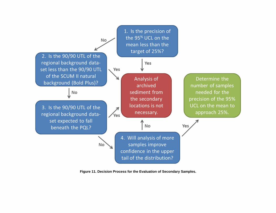
Figure 11. Decision Process for the Evaluation of Secondary Samples.

Appendices A-D, F, and G. Available at: www.ecy.wa.gov/biblio/1409339.html)

Appendix E. Data Tables

Port Gardner Regional Background

Phase II Data Tables

Table E‐1. Summary of Phase II Sediment Conventionals, Metals, and Carcinogenic Polycyclic Aromatic Hydrocarbons.Location ID PG‐01‐S Q PG‐04‐S Q PG‐05‐S Q PG‐08‐S Q PG‐09‐S Q PG‐10‐S Q PG‐10‐D QDate/Time 3/28/2013 15:48 3/26/2013 11:21 3/28/2013 13:18 3/26/2013 9:17 3/26/2013 11:42 3/28/2013 16:24 3/28/2013 16:24ConventionalsTotal Organic Carbon 0.738 2.09 1.98 2.01 2.03 0.524 0.58Total Solids 69.38 40.44 44.18 43.9 38.38 70.39 69.53Total Volatile Solids 2.45 6.49 5.95 6.08 7.09 2.23 2.22Preserved Total Solids 61.75 37.2 41.58 40.04 34.83 64.61 62.98Sulfide 1.61 UJ 55.9 J 74.7 J 13.9 J 33.9 J 4.94 J 3.02 JParticle/Grain Size, Phi Scale <‐1 0.1 U 0.1 0.1 U 0.2 0.1 U 0.1 U 0.1 UParticle/Grain Size, Phi Scale ‐1 to 0 0.1 0.7 0.1 0.4 0.1 0.1 0.1Particle/Grain Size, Phi Scale 0 to 1 0.5 1 0.6 0.4 0.3 0.5 0.5Particle/Grain Size, Phi Scale 1 to 2 2 0.8 1.1 0.9 0.4 1.3 1.4Particle/Grain Size, Phi Scale 2 to 3 24.2 1.5 2.1 1.4 0.3 11.7 11.3Particle/Grain Size, Phi Scale 3 to 4 48.1 6 10.8 8 1.7 59.3 59.7Particle/Grain Size, Phi Scale 4 to 5 10.8 12.8 18.5 16.1 7.7 13.9 14.2Particle/Grain Size, Phi Scale 5 to 6 4.3 17.7 16.9 16 15.9 4 3.8Particle/Grain Size, Phi Scale 6 to 7 2.9 14.1 12.9 13.9 17.3 2.5 2.4Particle/Grain Size, Phi Scale 7 to 8 1.7 11.5 9 10.5 15 1.6 1.5Particle/Grain Size, Phi Scale 8 to 9 1.2 9.6 8 8.5 11.6 1.1 1.1Particle/Grain Size, Phi Scale 9 to 10 1.1 8.3 6.7 8 10.1 1 1Particle/Grain Size, Phi Scale >10 3 16 13.3 15.7 19.7 3.1 3Particle/Grain Size, Fines (Silt/Clay) 25 90 85.3 88.7 97.2 27.1 27Metals (mg/kg DW)Arsenic 6 10.5 9.3 10.1 10.5 5.4 5.6Cadmium 0.18 0.35 J 0.26 0.32 J 0.33 J 0.3 0.42Mercury 0.04 0.12 0.13 0.12 0.13 0.04 0.05carcinogenic PAH (ug/kg DW)Benzo(a)anthracene 19.9 32.1 27.7 31.8 26.5 2.97 3.81Chrysene 21.9 40 47.9 46.9 34.6 4.19 7.06Benzo(b)fluoranthene 10.2 34.9 27.8 29.4 32.2 3.33 3.44Benzo(k)fluoranthene 6.31 15.6 14.6 18.1 13.4 1.67 J 1.85 JTotal Benzofluoranthenes 23.4 66.5 56.2 62.5 59.4 6.65 7.15Benzo(a)pyrene 19.2 32.5 26.1 29.7 28.7 2.69 3.05Indeno(1,2,3‐cd)pyrene 7.69 20 16.5 18 18.4 1.6 J 1.8 JDibenz(a,h)anthracene 2.9 4.74 J 4.1 4.32 J 4.02 J 0.868 U 0.799 UcPAH TEQ (0 DL) 24.1 43.6 35.6 40.3 38.5 3.69 4.21cPAH TEQ (1/2 DL) 24.1 43.6 35.6 40.3 38.5 3.73 4.25cPAH TEQ (1 DL) 24.1 43.6 35.6 40.3 38.5 3.78 4.29cPAH TEQ (KM) 24 44 36 40 38 4 AVG ‐‐* Insufficient fines were present for the full determination of silt and clay fractions. Only total fines are reported.

U‐the analytie was analyzed for, but was not detected above the reported sample quantitation limit

J‐the analyte was positively identified; the associated numerical value is the approximate concentration of the analyte in the sample

UJ‐the analyte was not detected above the reported sample quantitation limit. However, the reported quantitation limit is approximate.

L‐the detection frequency of compounds within a sample was <50%, the numeric value indicates the number of non‐detects

KM‐Kaplan‐Meier DW‐dry weight Q‐qualifier TEQ‐toxicity equivalent DL‐detection limit Avg‐average of field duplicates

Table E‐1. Summary of Phase II Sediment Conventionals, Metals, and Carcinogenic Polycyclic Aromatic Hydrocarbons (continued).Location ID PG‐10‐T Q PG‐12‐S Q PG‐15‐S Q PG‐17‐S Q PG‐21‐S Q PG‐23‐S Q PG‐27‐S QDate/Time 3/28/2013 16:24 3/27/2013 12:09 3/26/2013 9:45 3/26/2013 10:10 3/28/2013 12:59 3/29/2013 13:32 3/28/2013 14:50ConventionalsTotal Organic Carbon 0.733 1.74 1.59 1.73 2.44 1.59 1.72Total Solids 69.01 57.76 48.31 43.21 47.92 51.75 51.2Total Volatile Solids 2.19 4.01 5.26 5.88 5.79 5.63 5.78Preserved Total Solids 62.63 48.02 44.08 38.86 44.83 49 48.71Sulfide 2.23 J 5.01 J 2.31 UJ 6.42 J 135 J 28.6 32.8 JParticle/Grain Size, Phi Scale <‐1 0.3 13.4 0.1 U 0.1 0.5 0.5 0.1Particle/Grain Size, Phi Scale ‐1 to 0 0.1 5.8 0.3 0.4 0.3 0.1 0.1Particle/Grain Size, Phi Scale 0 to 1 0.4 7 1 0.8 1.4 0.5 0.5Particle/Grain Size, Phi Scale 1 to 2 1.4 10.6 7.8 1.1 2.9 0.7 1.1Particle/Grain Size, Phi Scale 2 to 3 12.1 10.7 7.5 1.5 6.9 1.9 2.3Particle/Grain Size, Phi Scale 3 to 4 59 8.1 10.5 12.8 10 13.3 16Particle/Grain Size, Phi Scale 4 to 5 14.5 5.2 15.5 16 14.4 30.7 22.4Particle/Grain Size, Phi Scale 5 to 6 3.4 4.9 11.9 12.3 14.6 19 16.9Particle/Grain Size, Phi Scale 6 to 7 2.4 7 9.6 11.9 11.7 9.9 10.1Particle/Grain Size, Phi Scale 7 to 8 1.5 7.1 9.1 9.4 9.7 6.2 6.9Particle/Grain Size, Phi Scale 8 to 9 1.1 5.9 6.9 8.9 7.9 4.4 5.8Particle/Grain Size, Phi Scale 9 to 10 1 4.8 6.3 8.7 6.7 4.3 5.5Particle/Grain Size, Phi Scale >10 2.9 9.5 13.6 16.1 12.9 8.6 12.2Particle/Grain Size, Fines (Silt/Clay) 26.7 44.4 72.9 83.2 78 83 79.9Metals (mg/kg DW)Arsenic ‐‐ 7.7 7.7 9 8.3 8.8 8.5Cadmium ‐‐ 0.22 J 0.29 J 0.31 J 0.27 0.43 0.38Mercury ‐‐ 0.09 0.1 0.11 0.1 0.1 0.1carcinogenic PAH (ug/kg DW)Benzo(a)anthracene ‐‐ 17.5 23.8 26.3 32 26.8 29.6Chrysene ‐‐ 22.7 33 35.9 44.8 34.8 41.7Benzo(b)fluoranthene ‐‐ 21.4 25.4 29.3 28.5 22.3 32Benzo(k)fluoranthene ‐‐ 9.08 14.4 16.9 15.5 14.5 12.9Total Benzofluoranthenes ‐‐ 40 52.1 60.1 58.9 47.8 57.5Benzo(a)pyrene ‐‐ 18.2 24.5 29 31.4 22.4 26.7Indeno(1,2,3‐cd)pyrene ‐‐ 12.4 15.2 19.3 18.9 11.7 16.9Dibenz(a,h)anthracene ‐‐ 2.27 J 3.67 J 4.57 J 4.57 3.47 3.81cPAH TEQ (0 DL) ‐‐ 24.7 33.1 39 41.8 30.6 36.6cPAH TEQ (1/2 DL) ‐‐ 24.7 33.1 39 41.8 30.6 36.6cPAH TEQ (1 DL) ‐‐ 24.7 33.1 39 41.8 30.6 36.6cPAH TEQ (KM) ‐‐ 25 33 39 42 31 37* Insufficient fines were present for the full determination of silt and clay fractions. Only total fines are reported.






Table E‐1. Summary of Phase II Sediment Conventionals, Metals, and Carcinogenic Polycyclic Aromatic Hydrocarbons (continued).Location ID PG‐28‐S Q PG‐31‐S Q PG‐34‐S Q PG‐51‐S Q PG‐52‐S Q PG‐53‐S Q PG‐54‐S QDate/Time 3/28/2013 19:36 3/27/2013 14:15 3/26/2013 10:39 4/22/2014 15:21 4/22/2014 10:24 4/22/2014 9:58 4/22/2014 14:10ConventionalsTotal Organic Carbon 0.861 0.416 1.32 0.866 J 0.315 J 1.54 J 2.26 JTotal Solids 69.26 67.19 41.15 50.5 68.26 64.03 51.05Total Volatile Solids 1.8 2.67 6.82 4.4 1.99 5.42 5.93Preserved Total Solids 69.31 63.24 39.35 ‐‐ ‐‐ ‐‐ ‐‐Sulfide 2.16 J 3.08 J 2.5 UJ ‐‐ ‐‐ ‐‐ ‐‐Particle/Grain Size, Phi Scale <‐1 0.1 U 0.1 U 0.1 U 1.9 0.1 U 0.4 0.6Particle/Grain Size, Phi Scale ‐1 to 0 0.1 0.1 0.1 5.8 0.1 0.7 1.1Particle/Grain Size, Phi Scale 0 to 1 0.7 0.7 0.7 7.5 0.5 3.8 1.6Particle/Grain Size, Phi Scale 1 to 2 11.7 9.9 1.5 13 2.7 6.6 3Particle/Grain Size, Phi Scale 2 to 3 72.8 41.3 2.2 14.7 52.1 11.3 2.4Particle/Grain Size, Phi Scale 3 to 4 9.9 23 6.6 12.5 38.3 23.7 10.1Particle/Grain Size, Phi Scale 4 to 5 2.1 5.9 11.8 7.8 2 23.4 26.9Particle/Grain Size, Phi Scale 5 to 6 0.5 3.7 15.6 7.8 0.5 11.2 18.9Particle/Grain Size, Phi Scale 6 to 7 0.3 3 15.4 6.9 0.7 5.8 9.9Particle/Grain Size, Phi Scale 7 to 8 0.2 2.7 11 5.8 0.6 3.5 6.4Particle/Grain Size, Phi Scale 8 to 9 0.3 2.3 9.8 5.1 0.4 2.2 4.5Particle/Grain Size, Phi Scale 9 to 10 0.3 2.2 8.7 4 0.4 2.2 4.5Particle/Grain Size, Phi Scale >10 1.1 5.1 16.5 7.3 1.6 5.3 9.9Particle/Grain Size, Fines (Silt/Clay) 4.8 24.8 88.8 44.7 6.2 53.5 81.1Metals (mg/kg DW)Arsenic 6.6 5.9 9.9 11.6 ‐‐ 7.8 9.1Cadmium 0.14 U 0.19 0.42 0.24 ‐‐ 0.29 0.51Mercury 0.03 U 0.05 0.12 0.04 U 0.03 U 0.07 0.09carcinogenic PAH (ug/kg DW)Benzo(a)anthracene 1.55 5.97 40.6 12.5 ‐‐ 44.1 32.4Chrysene 1.97 8.15 51.7 16.4 ‐‐ 48.9 41.6Benzo(b)fluoranthene 1.5 8.62 49.1 16.4 ‐‐ 29.8 31.3Benzo(k)fluoranthene 0.53 3.23 23 5.83 ‐‐ 14.1 15Total Benzofluoranthenes 2.58 15.1 92.4 28.1 ‐‐ 57.8 59.6Benzo(a)pyrene 1.07 6.23 40.2 13 ‐‐ 38.8 28.3Indeno(1,2,3‐cd)pyrene 0.68 4.42 28.4 10.6 ‐‐ 21.5 20.3Dibenz(a,h)anthracene 0.17 U 0.98 5.77 2.43 ‐‐ 5.55 4.96cPAH TEQ (0 DL) 1.52 8.63 55.4 17.9 ‐‐ 50.8 39.1cPAH TEQ (1/2 DL) 1.52 8.63 55.4 17.9 ‐‐ 50.8 39.1cPAH TEQ (1 DL) 1.53 8.63 55.4 17.9 ‐‐ 50.8 39.1cPAH TEQ (KM) 1.5 8.6 55 18 ‐‐ 51 39* Insufficient fines were present for the full determination of silt and clay fractions. Only total fines are reported.






Table E‐1. Summary of Phase II Sediment Conventionals, Metals, and Carcinogenic Polycyclic Aromatic Hydrocarbons (continued).Location ID PG‐55‐S Q PG‐56‐S Q PG‐57‐S Q PG‐58‐S Q PG‐59‐S Q PG‐60‐S Q PG‐61‐S QDate/Time 4/23/2014 12:40 4/23/2014 10:32 4/22/2014 13:23 4/22/2014 10:46 4/22/2014 11:17 4/23/2014 9:11 4/23/2014 13:13ConventionalsTotal Organic Carbon 2.05 J 0.424 J 0.504 J 1.02 J 0.15 J 2.11 J 0.268 JTotal Solids 38.08 67.84 72.32 58.15 75.76 55.21 41.18Total Volatile Solids 6.94 2.45 2.46 5.39 1.15 6.73 6.18Preserved Total Solids ‐‐ ‐‐ ‐‐ ‐‐ ‐‐ ‐‐ ‐‐Sulfide ‐‐ ‐‐ ‐‐ ‐‐ ‐‐ ‐‐ ‐‐Particle/Grain Size, Phi Scale <‐1 0.1 U 7.6 0.5 0.1 U 0.7 0.4 0.1 UParticle/Grain Size, Phi Scale ‐1 to 0 0.2 3.7 1.1 0.4 3.6 1.7 1Particle/Grain Size, Phi Scale 0 to 1 0.6 4.4 12.1 0.6 15.3 4.6 1.4Particle/Grain Size, Phi Scale 1 to 2 0.8 15.3 33.2 1.2 31.7 13.2 1.2Particle/Grain Size, Phi Scale 2 to 3 0.5 22.9 15.1 6.3 27 15.7 3.7Particle/Grain Size, Phi Scale 3 to 4 3 13 23.8 23.1 18 11.5 9.6Particle/Grain Size, Phi Scale 4 to 5 10.2 8.3 5.6 28 ‐‐ 13.6 12.1Particle/Grain Size, Phi Scale 5 to 6 16.8 5.1 2.1 15 ‐‐ 12.1 15.8Particle/Grain Size, Phi Scale 6 to 7 17.3 4.4 1.2 8 ‐‐ 7 13.1Particle/Grain Size, Phi Scale 7 to 8 14.5 3.8 1.1 5.2 ‐‐ 4.9 10.9Particle/Grain Size, Phi Scale 8 to 9 9.9 2.8 1 2.7 ‐‐ 3.7 9.4Particle/Grain Size, Phi Scale 9 to 10 10.6 2.9 1 3.1 ‐‐ 3.8 7.8Particle/Grain Size, Phi Scale >10 15.4 5.7 2.3 6.4 ‐‐ 7.9 13.9Particle/Grain Size, Fines (Silt/Clay) 94.8 33.1 14.3 68.4 3.7 * 53 83Metals (mg/kg DW)Arsenic 8.5 ‐‐ 4.5 8.6 2.9 10.1 8.9Cadmium 0.36 ‐‐ 0.19 0.36 0.13 U 0.61 0.39Mercury 0.11 0.03 0.03 0.08 0.03 U 0.16 0.11carcinogenic PAH (ug/kg DW)Benzo(a)anthracene 34.9 ‐‐ 21.4 J 31.2 2.24 J 50.3 28Chrysene 47.4 ‐‐ 23.2 44.5 3.06 J 135 35.5Benzo(b)fluoranthene 40.4 ‐‐ 16.1 27.7 2.64 32.6 31.8Benzo(k)fluoranthene 17.4 ‐‐ 7.05 12.3 1.18 18.6 14.6Total Benzofluoranthenes 73.9 ‐‐ 30.3 50.9 4.86 64.7 59.5Benzo(a)pyrene 34.9 ‐‐ 16.9 22.3 2.09 J 32.6 28.3Indeno(1,2,3‐cd)pyrene 26.3 ‐‐ 9.61 13.7 1.5 21.6 21.2Dibenz(a,h)anthracene 5.79 ‐‐ 2.43 3.65 0.39 J 5.56 4.89cPAH TEQ (0 DL) 47.9 ‐‐ 22.8 31.6 2.92 46.8 38.7cPAH TEQ (1/2 DL) 47.9 ‐‐ 22.8 31.6 2.92 46.8 38.7cPAH TEQ (1 DL) 47.9 ‐‐ 22.8 31.6 2.92 46.8 38.7cPAH TEQ (KM) 48 ‐‐ 23 32 2.9 47 39* Insufficient fines were present for the full determination of silt and clay fractions. Only total fines are reported.






Table E‐1. Summary of Phase II Sediment Conventionals, Metals, and Carcinogenic Polycyclic Aromatic Hydrocarbons (continued).Location ID PG‐62‐S Q PG‐63‐S Q PG‐64‐S Q PG‐65‐S Q PG‐65‐D Q PG‐65‐T QDate/Time 4/22/2014 13:46 4/23/2014 13:42 4/22/2014 12:03 4/23/2014 11:08 4/23/2014 11:08 4/23/2014 11:08ConventionalsTotal Organic Carbon 1.28 J 1.45 J 0.431 J 1.26 J 1.4 J 1.13 JTotal Solids 68.31 48.95 73.23 61.52 61.02 61.79Total Volatile Solids 2.64 5.25 1.46 4.82 4.08 4.13Preserved Total Solids ‐‐ ‐‐ ‐‐ ‐‐ ‐‐ ‐‐Sulfide ‐‐ ‐‐ ‐‐ ‐‐ ‐‐ ‐‐Particle/Grain Size, Phi Scale <‐1 1.5 0.1 U 0.1 0.1 U 0.1 U 0.1 UParticle/Grain Size, Phi Scale ‐1 to 0 0.7 0.3 0.2 0.4 0.4 0.3Particle/Grain Size, Phi Scale 0 to 1 1.9 0.8 1.2 0.6 0.6 0.7Particle/Grain Size, Phi Scale 1 to 2 28.8 3.5 10 1.3 1.5 1.5Particle/Grain Size, Phi Scale 2 to 3 35 13.1 52.4 6.4 8.1 7.5Particle/Grain Size, Phi Scale 3 to 4 7.9 13.1 29.5 28.3 25.9 26.8Particle/Grain Size, Phi Scale 4 to 5 8.3 15.2 1.8 29.8 29.9 31Particle/Grain Size, Phi Scale 5 to 6 4.8 13.9 0.6 12.1 12.6 11.5Particle/Grain Size, Phi Scale 6 to 7 3.2 10.9 0.7 5.5 5.7 5.5Particle/Grain Size, Phi Scale 7 to 8 2.1 7.6 0.6 3.8 3.6 3.6Particle/Grain Size, Phi Scale 8 to 9 1.6 5.3 0.7 2.6 2.6 3.5Particle/Grain Size, Phi Scale 9 to 10 1.6 5.9 0.7 2.8 2.7 2.1Particle/Grain Size, Phi Scale >10 2.7 10.5 1.6 6.3 6.6 6.1Particle/Grain Size, Fines (Silt/Clay) 24.2 69.2 6.6 63 63.6 63.3Metals (mg/kg DW)Arsenic 3.7 ‐‐ 3.3 6.6 6.1 ‐‐Cadmium 0.24 ‐‐ 0.17 0.35 0.3 ‐‐Mercury 0.04 0.09 0.03 U 0.06 0.14 ‐‐carcinogenic PAH (ug/kg DW)Benzo(a)anthracene 18.1 ‐‐ 10.1 21.9 20.5 ‐‐Chrysene 24.1 ‐‐ 17.2 26.9 26.2 ‐‐Benzo(b)fluoranthene 16.5 ‐‐ 8.19 22.2 21.1 ‐‐Benzo(k)fluoranthene 6.79 ‐‐ 4.28 9.49 8.86 ‐‐Total Benzofluoranthenes 29.9 ‐‐ 16.3 40.8 38.4 ‐‐Benzo(a)pyrene 15.3 ‐‐ 7.8 21.6 20.1 ‐‐Indeno(1,2,3‐cd)pyrene 9.33 ‐‐ 4.59 14.4 13 ‐‐Dibenz(a,h)anthracene 2.13 ‐‐ 1.09 3.15 3.02 ‐‐cPAH TEQ (0 DL) 20.8 ‐‐ 10.8 29 27 ‐‐cPAH TEQ (1/2 DL) 20.8 ‐‐ 10.8 29 27 ‐‐cPAH TEQ (1 DL) 20.8 ‐‐ 10.8 29 27 ‐‐cPAH TEQ (KM) 21 ‐‐ 11 28 AVG ‐‐ ‐‐* Insufficient fines were present for the full determination of silt and clay fractions. Only total fines are reported.






Table E‐2. Summary of Phase II Dioxin/Furan Congener Data.Location ID PG‐01‐S Q PG‐04‐S Q PG‐05‐S Q PG‐08‐S Q PG‐09‐S Q PG‐10‐S Q PG‐10‐D Q PG‐12‐S QDate/Time 3/28/2013 15:48 3/26/2013 11:21 3/28/2013 13:18 3/26/2013 9:17 3/26/2013 11:42 3/28/2013 16:24 3/28/2013 16:24 3/27/2013 12:09Dioxin/Furan Congeners (ng/kg DW)2,3,7,8‐TCDD 0.102 J 0.29 0.348 U 0.347 0.325 0.1 U 0.142 U 0.2351,2,3,7,8‐PECDD 0.129 U 0.787 J 0.858 J 0.851 J 0.822 J 0.188 J 0.216 J 0.631 J1,2,3,4,7,8‐HXCDD 0.187 J 0.881 J 0.861 J 0.868 J 0.844 J 0.179 UJ 0.272 J 0.638 J1,2,3,6,7,8‐HXCDD 0.652 J 3.62 3.4 3.65 3.66 0.83 J 0.862 J 2.91,2,3,7,8,9‐HXCDD 0.566 J 2.76 2.8 2.97 2.97 0.69 J 0.859 J 2.261,2,3,4,6,7,8‐HPCDD 8.76 50.4 50.3 47.2 57.4 10.4 11.5 33.9OCDD 75.4 400 415 380 535 92.8 97.4 2602,3,7,8‐TCDF 0.53 2.2 2.59 2.41 2.44 0.663 0.58 1.741,2,3,7,8‐PECDF 0.11 U 0.505 J 0.54 J 0.606 J 0.545 J 0.099 U 0.101 J 0.412 J2,3,4,7,8‐PECDF 0.155 J 0.978 0.883 J 0.927 J 0.969 J 0.175 J 0.177 U 0.713 J1,2,3,4,7,8‐HXCDF 0.134 J 1.03 1.09 1.07 1.2 0.205 J 0.237 J 0.821 J1,2,3,6,7,8‐HXCDF 0.103 J 0.647 J 0.642 J 0.617 J 0.664 J 0.111 U 0.159 J 0.445 J1,2,3,7,8,9‐HXCDF 0.0475 U 0.061 U 0.062 U 0.071 U 0.066 U 0.0512 UJ 0.053 J 0.049 J2,3,4,6,7,8‐HXCDF 0.107 U 0.622 J 0.64 J 0.603 J 0.651 J 0.057 J 0.153 U 0.478 J1,2,3,4,6,7,8‐HPCDF 1.36 10.6 9.93 8.82 12.2 1.97 1.83 7.341,2,3,4,7,8,9‐HPCDF 0.087 J 0.519 J 0.628 J 0.516 J 0.592 J 0.113 J 0.18 J 0.502 JOCDF 3.04 20.9 J 25.2 18.4 J 39.5 J 5.29 4.59 13.7 JDx/F TEQ (0 DL) 0.491 3.3 3.08 3.4 3.57 0.639 0.687 2.52Dx/F TEQ (1/2 DL) 0.565 3.31 3.26 3.4 3.57 0.708 0.792 2.52Dx/F TEQ (1 DL) 0.639 3.31 3.44 3.41 3.58 0.776 0.897 2.52Dx/F TEQ (KM) 0.62 L 3.3 3.2 3.4 3.6 0.71 AVG ‐‐ 2.5*total PCBs represents the sum of all detected congeners






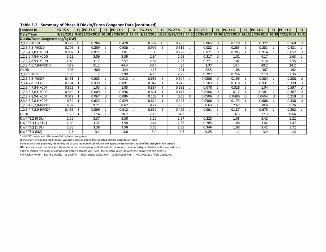
Table E‐2. Summary of Phase II Dioxin/Furan Congener Data (continued).Location ID PG‐15‐S Q PG‐17‐S Q PG‐21‐S Q PG‐23‐S Q PG‐27‐S Q PG‐28‐S Q PG‐31‐S Q PG‐34‐S Q PG‐51‐S QDate/Time 3/26/2013 9:45 3/26/2013 10:10 3/28/2013 12:59 3/29/2013 13:32 3/28/2013 14:50 3/28/2013 19:36 3/27/2013 14:15 3/26/2013 10:39 4/22/2014 15:21Dioxin/Furan Congeners (ng/kg DW)2,3,7,8‐TCDD 0.278 U 0.284 0.478 0.367 U 0.266 0.065 U 0.129 J 0.322 0.169 U1,2,3,7,8‐PECDD 0.706 J 0.859 J 0.936 J 0.909 J 0.619 J 0.082 J 0.265 J 0.801 J 0.421 J1,2,3,4,7,8‐HXCDD 0.807 J 0.877 J 1.01 1.09 0.722 J 0.071 U 0.283 J 0.914 J 0.652 U1,2,3,6,7,8‐HXCDD 3.12 3.59 3.39 2.94 2.63 0.317 U 1.02 4.17 1.63 J1,2,3,7,8,9‐HXCDD 2.49 3.17 2.57 2.84 2.23 0.271 J 1.02 3.16 1.55 J1,2,3,4,6,7,8‐HPCDD 40.9 51.2 44.4 50.4 35 3.37 14.4 49.2 24.2OCDD 306 400 324 415 291 22.5 108 387 1622,3,7,8‐TCDF 1.85 2 2.99 4.15 2.25 0.297 0.754 2.19 1.351,2,3,7,8‐PECDF 0.461 J 0.535 J 0.613 J 0.689 J 0.504 J 0.0506 U 0.196 J 0.584 J 0.288 U2,3,4,7,8‐PECDF 0.784 J 0.939 J 0.891 J 0.942 J 0.746 J 0.103 J 0.318 J 0.931 J 0.339 U1,2,3,4,7,8‐HXCDF 0.823 J 1.03 J 1.05 0.887 J 0.692 J 0.078 J 0.328 J 1.04 0.597 U1,2,3,6,7,8‐HXCDF 0.519 J 0.609 J 0.696 J 0.631 J 0.447 J 0.0506 U 0.17 J 0.581 J 0.387 U1,2,3,7,8,9‐HXCDF 0.072 J 0.067 U 0.086 J 0.103 J 0.05 U 0.0506 U 0.0496 U 0.0654 U 0.219 U2,3,4,6,7,8‐HXCDF 0.52 J 0.623 J 0.629 J 0.612 J 0.443 J 0.0506 U 0.175 J 0.666 J 0.336 U1,2,3,4,6,7,8‐HPCDF 6.97 9.71 8.62 8.22 6.35 0.63 J 2.67 10.4 5.261,2,3,4,7,8,9‐HPCDF 0.495 J 0.569 J 0.612 J 0.619 J 0.455 J 0.061 J 0.187 J 0.675 J 0.262 JOCDF 13.8 J 17.4 J 20.7 20.3 14.3 1.1 J 6.5 22.3 8.64Dx/F TEQ (0 DL) 2.55 3.37 3.58 3.26 2.57 0.225 1.08 3.42 1.22Dx/F TEQ (1/2 DL) 2.69 3.37 3.58 3.44 2.58 0.285 1.08 3.42 1.47Dx/F TEQ (1 DL) 2.83 3.38 3.58 3.63 2.58 0.346 1.08 3.42 1.72Dx/F TEQ (KM) 2.6 3.4 3.6 3.4 2.6 0.25 1.1 3.4 1.3*total PCBs represents the sum of all detected congeners






Table E‐2. Summary of Phase II Dioxin/Furan Congener Data (continued).Location ID PG‐53‐S Q PG‐54‐S Q PG‐55‐S Q PG‐57‐S Q PG‐58‐S Q PG‐59‐S Q PG‐60‐S Q PG‐61‐S QDate/Time 4/22/2014 9:58 4/22/2014 14:10 4/23/2014 12:40 4/22/2014 13:23 4/22/2014 10:46 4/22/2014 11:17 4/23/2014 9:11 4/23/2014 13:13Dioxin/Furan Congeners (ng/kg DW)2,3,7,8‐TCDD 0.161 J 0.135 U 0.313 0.092 U 0.193 J 0.0496 U 0.482 0.246 U1,2,3,7,8‐PECDD 0.287 J 0.67 J 1.04 0.332 J 0.423 J 0.056 U 1.14 0.829 J1,2,3,4,7,8‐HXCDD 0.377 J 0.86 U 0.992 U 0.313 U 0.517 J 0.0803 U 1.09 1.181,2,3,6,7,8‐HXCDD 1.16 2.3 4.43 0.981 1.53 0.214 J 3.17 3.441,2,3,7,8,9‐HXCDD 1.13 2.1 3.93 0.972 J 1.64 0.242 J 2.93 3.081,2,3,4,6,7,8‐HPCDD 18.8 34.2 60.4 11 28.4 3.57 33.8 44OCDD 156 268 453 72.4 227 28.6 222 3372,3,7,8‐TCDF 1.47 2.7 3.3 1.42 1.41 0.311 4.13 2.371,2,3,7,8‐PECDF 0.122 J 0.44 J 0.703 J 0.234 J 0.228 U 0.05 U 0.876 J 0.482 J2,3,4,7,8‐PECDF 0.278 U 0.683 J 1.23 U 0.362 U 0.342 U 0.076 J 1.38 0.615 J1,2,3,4,7,8‐HXCDF 0.44 J 0.606 J 1.27 0.325 J 0.433 U 0.0687 U 1.07 U 0.866 J1,2,3,6,7,8‐HXCDF 0.22 U 0.54 J 0.789 J 0.26 U 0.312 J 0.0687 U 0.921 J 0.512 J1,2,3,7,8,9‐HXCDF 0.0523 U 0.0842 U 0.0903 U 0.0777 U 0.0726 U 0.0687 U 0.099 U 0.0938 U2,3,4,6,7,8‐HXCDF 0.283 U 0.439 U 0.807 J 0.192 U 0.338 U 0.075 U 0.792 J 0.594 U1,2,3,4,6,7,8‐HPCDF 3.64 6.88 12.5 2.44 4.9 0.585 J 6.87 8.251,2,3,4,7,8,9‐HPCDF 0.299 J 0.59 J 0.957 J 0.21 U 0.499 J 0.064 J 0.541 J 0.705 JOCDF 6.85 14.7 24 3.82 11.3 1.17 J 11.7 18.5Dx/F TEQ (0 DL) 1.19 2.21 3.71 0.866 1.57 0.151 3.85 2.81Dx/F TEQ (1/2 DL) 1.26 2.35 3.95 1.01 1.66 0.222 3.91 2.97Dx/F TEQ (1 DL) 1.32 2.49 4.19 1.15 1.76 0.294 3.96 3.12Dx/F TEQ (KM) 1.2 2.3 3.9 0.93 1.6 0.23 L 3.9 2.9*total PCBs represents the sum of all detected congeners






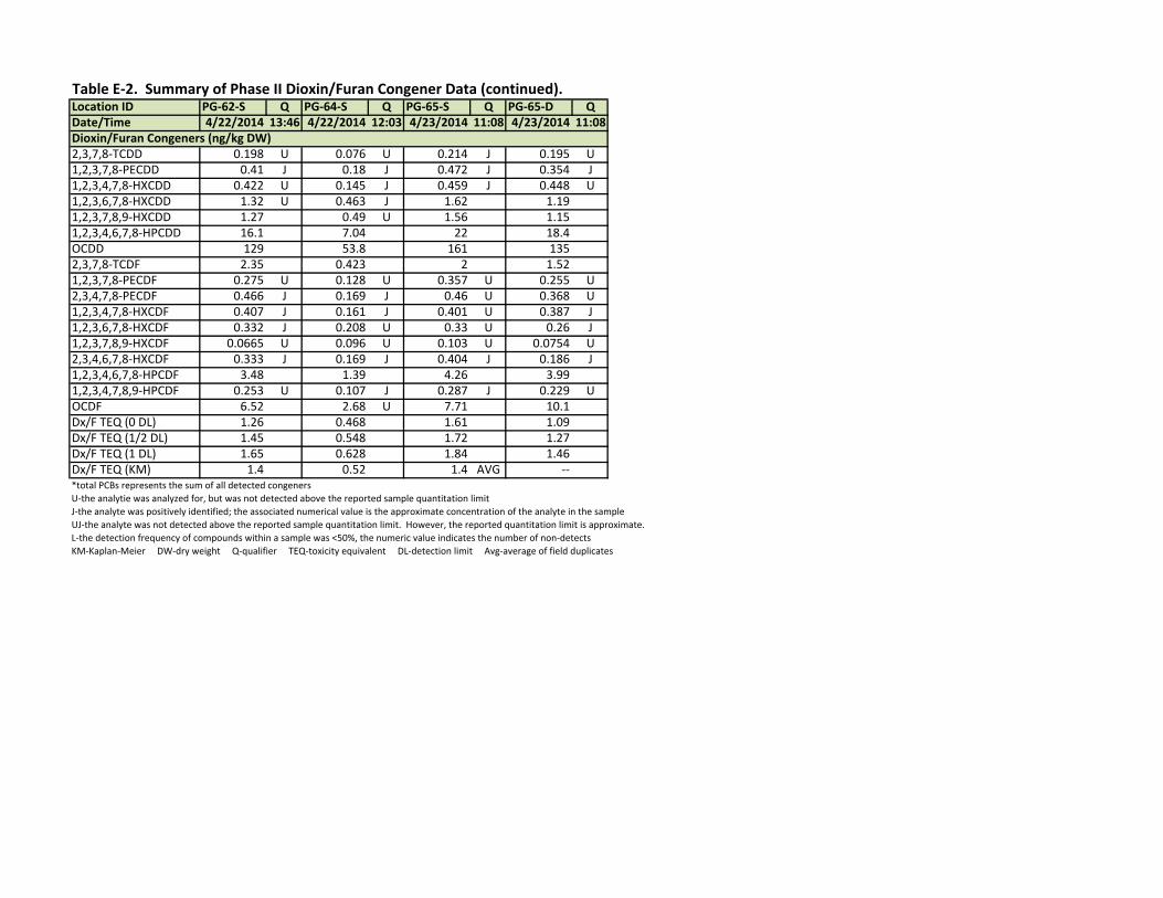
Table E‐2. Summary of Phase II Dioxin/Furan Congener Data (continued).Location ID PG‐62‐S Q PG‐64‐S Q PG‐65‐S Q PG‐65‐D QDate/Time 4/22/2014 13:46 4/22/2014 12:03 4/23/2014 11:08 4/23/2014 11:08Dioxin/Furan Congeners (ng/kg DW)2,3,7,8‐TCDD 0.198 U 0.076 U 0.214 J 0.195 U1,2,3,7,8‐PECDD 0.41 J 0.18 J 0.472 J 0.354 J1,2,3,4,7,8‐HXCDD 0.422 U 0.145 J 0.459 J 0.448 U1,2,3,6,7,8‐HXCDD 1.32 U 0.463 J 1.62 1.191,2,3,7,8,9‐HXCDD 1.27 0.49 U 1.56 1.151,2,3,4,6,7,8‐HPCDD 16.1 7.04 22 18.4OCDD 129 53.8 161 1352,3,7,8‐TCDF 2.35 0.423 2 1.521,2,3,7,8‐PECDF 0.275 U 0.128 U 0.357 U 0.255 U2,3,4,7,8‐PECDF 0.466 J 0.169 J 0.46 U 0.368 U1,2,3,4,7,8‐HXCDF 0.407 J 0.161 J 0.401 U 0.387 J1,2,3,6,7,8‐HXCDF 0.332 J 0.208 U 0.33 U 0.26 J1,2,3,7,8,9‐HXCDF 0.0665 U 0.096 U 0.103 U 0.0754 U2,3,4,6,7,8‐HXCDF 0.333 J 0.169 J 0.404 J 0.186 J1,2,3,4,6,7,8‐HPCDF 3.48 1.39 4.26 3.991,2,3,4,7,8,9‐HPCDF 0.253 U 0.107 J 0.287 J 0.229 UOCDF 6.52 2.68 U 7.71 10.1Dx/F TEQ (0 DL) 1.26 0.468 1.61 1.09Dx/F TEQ (1/2 DL) 1.45 0.548 1.72 1.27Dx/F TEQ (1 DL) 1.65 0.628 1.84 1.46Dx/F TEQ (KM) 1.4 0.52 1.4 AVG ‐‐*total PCBs represents the sum of all detected congeners






Table E‐3. Summary of Phase II Polychlorinated Biphenyl (PCB) Congener Data.Location ID PG‐01‐S Q PG‐04‐S Q PG‐05‐S Q PG‐08‐S Q PG‐09‐S Q PG‐10‐S QDate/Time 3/28/2013 15:48 3/26/2013 11:21 3/28/2013 13:18 3/26/2013 9:17 3/26/2013 11:42 3/28/2013 16:24PCB Congeners (ng/kg DW)PCB‐001 2.84 17 21.1 15.3 22 4.55PCB‐002 7.41 16.8 24.4 20.1 19.4 7.69PCB‐003 4.4 11.4 17.5 13.1 13.2 5.95PCB‐004 3.27 21.5 25.5 29.6 23.3 6.12PCB‐005 0.209 J 0.725 1.02 1.07 U 0.893 U 0.349 JPCB‐006 2.11 9.99 10.9 13.1 9.24 3.9PCB‐007 0.874 4.9 U 4.49 4.45 3.9 1.59PCB‐008 13.7 76.4 76.5 80.4 69.3 23.3PCB‐009 0.561 2.51 2.65 3.24 2 U 0.939PCB‐010 0.154 U 1.04 1.06 1.09 U 0.862 0.32 UPCB‐011 14.4 35.3 38.8 30.4 41.7 17.7PCB‐012/013 5.02 CUJ 9.43 C 9.24 CUJ 9.22 C 15.7 CU 3.95 CUJPCB‐014 0.442 U 0.736 U 1.04 U 0.693 U 0.624 U 0.447 UPCB‐015 20.5 69.5 81.3 76.3 73.7 24.4PCB‐016 6.55 22 28.9 35.2 18.8 13.4PCB‐017 7.99 39.4 43.6 51.7 32.5 16.2PCB‐018/030 15.3 C 49.2 C 61.7 C 83.6 C 40.8 C 28.3 CPCB‐019 1.3 6.31 7.39 9.42 6.14 2.53PCB‐020/028 64.7 C 206 C 233 C 227 C 187 C 103 CPCB‐021/033 19.4 C 54.6 C 66.8 C 72.3 C 48 C 36.1 CPCB‐022 15.3 45 54.9 56 38.6 26.5PCB‐023 0.0879 U 0.161 U 0.176 J 0.238 U 0.12 U 0.093 UPCB‐024 0.16 J 0.712 0.676 1.37 U 0.515 U 0.397 UPCB‐025 3.68 13.5 14.5 14.7 12.3 5.79PCB‐026/029 6.59 C 23.4 C 27.9 C 27.4 C 20.5 C 11.4 CPCB‐027 1.1 J 6.49 6.32 J 8.29 6.35 2.09 JPCB‐031 39.4 121 140 144 102 68PCB‐032 6.54 38 42.7 47.5 33.1 12.5PCB‐034 0.289 U 0.902 1.13 0.951 0.112 U 0.47PCB‐035 1.74 6.39 6.96 6.32 6.04 2.32PCB‐036 0.442 1.51 1.83 1.42 1.43 0.532PCB‐037 19.7 78.1 86.5 88.2 77.4 28.2PCB‐038 0.211 U 0.619 0.682 0.541 0.569 U 0.255 JPCB‐039 0.479 1.51 1.72 1.7 1.34 0.655PCB‐040/041/071 22.9 C 101 C 100 C 112 C 96 C 42 CPCB‐042 12.3 55.1 53.2 58.9 52.9 22.4PCB‐043 1.24 5.39 5.43 7.75 5.7 U 2.29PCB‐044/047/065 44.5 C 188 C 198 C 227 C 185 C 78.3 CPCB‐045/051 5.39 C 25.1 C 25.6 C 29.7 C 23.6 C 9.43 CPCB‐046 1.95 8.52 8.62 10.1 8.49 3.19PCB‐048 7.98 30.6 31.8 35.8 27.7 14.2PCB‐049/069 30 C 140 C 144 C 158 C 133 C 53.9 CPCB‐050/053 4.51 C 22.2 C 22 C 25.4 C 21.2 C 7.61 CPCB‐052 54.5 203 223 294 210 93.1PCB‐054 0.375 U 0.449 0.425 0.449 U 0.421 U 0.401 UPCB‐055 0.838 U 2.9 2.4 0.335 U 2.34 0.974PCB‐056 28.5 86.3 102 103 87 46.9PCB‐057 0.818 U 0.88 U 1.09 0.88 0.894 U 0.813 UPCB‐058 0.833 U 0.915 1.19 0.889 0.913 U 0.827 UPCB‐059/062/075 3.95 C 18.2 C 18.5 C 19.2 C 17.1 C 7.11 CPCB‐060 14.7 47 55.3 55.8 45.1 23.7PCB‐061/070/074/076 107 C 359 C 411 C 439 C 337 C 176 CPCB‐063 2.55 9.43 9.23 9.32 8.49 4.22 UPCB‐064 19.2 76.8 81.4 92 73.4 35.4PCB‐066 55.4 224 235 243 210 90.3PCB‐067 2.02 6.94 7.67 7.1 6.31 U 3.03PCB‐068 0.791 U 2.62 2.69 2.35 U 2.31 0.912PCB‐072 1.03 U 3.77 3.77 3.29 3.43 1.52PCB‐073 0.415 U 0.412 U 0.624 0.0689 U 0.399 U 0.463 U

Location ID PG‐01‐S Q PG‐04‐S Q PG‐05‐S Q PG‐08‐S Q PG‐09‐S Q PG‐10‐S QDate/Time 3/28/2013 15:48 3/26/2013 11:21 3/28/2013 13:18 3/26/2013 9:17 3/26/2013 11:42 3/28/2013 16:24PCB‐077 8.73 37 40 39.3 37.6 12.7PCB‐078 0.799 U 0.766 U 0.277 U 0.306 U 0.868 U 0.793 UPCB‐079 1.01 U 5.56 4.57 6.64 4.87 1.5PCB‐080 0.758 U 0.727 U 0.263 U 0.291 U 0.824 U 0.753 UPCB‐081 0.866 U 1.49 1.48 U 1.71 U 1.35 U 0.85 UPCB‐082 7.52 37.3 39.2 57.5 37.8 11.1 JPCB‐083/099 48.3 C 273 C 251 C 319 C 274 C 73.7 CPCB‐084 14 81.2 79.8 114 91.4 23.3PCB‐085/116/117 14.6 C 73.4 C 72.9 C 92.2 C 80 C 22.9 CPCB‐087/097/108/119/125 48.5 C 238 C 244 C 323 C 256 C 75.5 CPCB‐088/091 8.78 C 52.8 C 50.6 C 66.1 C 54.7 C 14.5 CPCB‐089 0.688 U 4.47 4.1 5.48 4.96 1.19PCB‐090/101/113 72 C 393 C 382 C 504 C 402 C 119 CPCB‐092 14.1 69.5 69.6 94.8 71.1 23PCB‐093/095/098/100/102 50.6 C 263 C 268 C 367 C 287 C 79 CPCB‐094 0.437 2.15 2.01 2.24 2.06 U 0.563PCB‐096 0.331 J 2.15 1.95 2.72 2.59 0.598PCB‐103 0.944 6.49 5.67 5.97 6.09 1.49PCB‐104 0.0568 U 0.12 J 0.117 U 0.093 U 0.086 J 0.0463 UPCB‐105 34.4 164 178 209 169 48.7PCB‐106 0.189 U 0.295 U 0.225 U 0.689 U 0.479 U 0.225 UPCB‐107/124 2.77 C 13.8 C 14.8 C 18.1 C 13.9 C 4.02 CPCB‐109 6.02 31.1 33.7 37.4 32.2 8.76PCB‐110/115 81.1 C 400 C 412 C 544 C 432 C 127 CPCB‐111 0.114 J 0.579 0.526 0.521 0.132 U 0.208 JPCB‐112 0.0671 U 0.135 U 0.117 U 0.0719 U 0.129 U 0.0596 UPCB‐114 1.76 7.34 8.05 10.1 7.2 2.45PCB‐118 78.8 392 425 497 395 116PCB‐120 0.601 U 3.27 2.77 2.73 3.05 0.908PCB‐121 0.0675 U 0.205 U 0.209 J 0.226 U 0.181 U 0.0599 UPCB‐122 0.94 4.71 4.56 6.2 4.52 1.32PCB‐123 1.41 U 7.73 7.84 U 8.97 7.2 2.1 UPCB‐126 0.32 J 2.59 U 2.55 2.58 2.58 0.509PCB‐127 0.181 U 0.274 U 0.216 U 0.64 U 0.445 U 0.637PCB‐128/166 13.1 C 85.3 C 83.2 C 106 C 86.9 C 19.6 CPCB‐129/138/160/163 87.1 C 566 C 549 C 635 C 571 C 137 CPCB‐130 5.19 37.9 35.1 40.3 37.8 8.15PCB‐131 0.774 U 5.74 5.16 7.31 5.6 1.37 UPCB‐132 23.6 168 155 197 181 39.3PCB‐133 1.61 10 9.06 9.91 9.69 2.59PCB‐134/143 3.56 C 25.8 C 22.8 C 29 C 27 C 101 CJPCB‐135/151/154 27.2 C 184 C 158 C 200 C 189 C 45.1 CPCB‐136 8.48 61.9 52.5 65.6 60.8 14.3PCB‐137 2.63 15.5 14.4 18 14.9 4.51PCB‐139/140 1.51 C 11 C 9.54 C 11.8 C 11.1 C 2.33 CPCB‐141 11 48.6 53.3 63.6 47.2 19.2PCB‐142 0.27 U 0.665 U 0.461 U 0.464 U 0.56 U 0.251 UPCB‐144 3.15 20.4 18.8 23.6 21.7 5.28PCB‐145 0.0848 U 0.196 U 0.239 U 0.235 U 0.245 J 0.0681 UPCB‐146 15.6 95.8 90.1 117 80.5 23.6PCB‐147/149 55 C 391 C 373 C 447 C 408 C 91.2 CPCB‐148 0.212 U 2.08 1.6 1.84 0.98 0.339 JPCB‐150 0.249 U 2.04 1.6 1.68 1.94 0.45PCB‐152 0.095 J 0.51 U 0.323 J 0.503 U 0.46 U 0.167 UPCB‐153/168 76.9 C 506 C 491 C 535 C 483 C 126 CPCB‐155 0.0596 U 0.231 J 0.161 J 0.198 U 0.159 J 0.047 JPCB‐156/157 8.64 C 48.1 C 51.5 C 64.9 C 49.4 C 13.4 CPCB‐158 7.98 45.5 44.6 55.4 46.1 12.3PCB‐159 0.964 U 5.67 5.07 5.53 5.18 1.3PCB‐161 0.183 U 0.432 U 0.314 U 0.302 U 0.364 U 0.171 UPCB‐162 0.298 U 1.66 1.83 2.11 1.66 0.383

Location ID PG‐01‐S Q PG‐04‐S Q PG‐05‐S Q PG‐08‐S Q PG‐09‐S Q PG‐10‐S QDate/Time 3/28/2013 15:48 3/26/2013 11:21 3/28/2013 13:18 3/26/2013 9:17 3/26/2013 11:42 3/28/2013 16:24PCB‐164 5.94 34.3 35.4 41.6 34.6 9.34PCB‐165 0.211 U 0.935 0.932 0.877 0.862 0.197 UPCB‐167 3.09 20.1 20.3 24 19.3 4.61PCB‐169 0.187 U 0.715 U 0.54 U 0.604 U 0.644 U 0.181 UPCB‐170 17.7 94 99.5 104 89.4 28.5PCB‐171/173 6.01 C 43.7 C 38.9 C 44.9 C 40.9 C 9.41 CPCB‐172 3.29 17.3 17 19.6 16.2 4.86PCB‐174 16.3 117 101 117 109 26.2PCB‐175 0.884 7.16 5.73 6.61 6.33 1.37PCB‐176 2.42 19.9 15.9 18.6 18.2 3.8PCB‐177 12.1 99.3 83.5 95.3 96 18.3PCB‐178 4.88 43.6 33.7 38.4 38.2 7.52PCB‐179 8.34 67.1 55.7 63.6 62.6 13.1PCB‐180/193 38.9 C 181 C 202 C 209 C 169 C 62.8 CPCB‐181 0.158 U 1.38 1.21 1.64 1.38 0.234 JPCB‐182 0.212 U 1.19 1 1.25 U 1.02 0.289 UPCB‐183/185 13.8 C 104 C 84.5 C 97.4 C 93.4 C 21.3 CPCB‐184 0.118 U 0.425 0.415 0.437 0.347 J 0.0674 UPCB‐186 0.127 U 0.216 U 0.107 U 0.113 U 0.252 U 0.0729 UPCB‐187 29.9 236 196 218 222 44.3PCB‐188 0.116 U 0.729 U 0.598 0.697 U 0.774 U 0.2 JPCB‐189 0.863 U 3.89 4.36 4.51 3.82 1.29PCB‐190 3.38 17.2 19.8 22.9 18 5.21PCB‐191 0.801 4.54 4.43 5 4.02 1.13 UPCB‐192 0.135 U 0.231 U 0.102 U 0.121 U 0.27 U 0.0774 UPCB‐194 9.09 41.9 55.1 54.1 44.6 13.7PCB‐195 3.39 20.8 25.3 24.7 21.6 5.17PCB‐196 5.31 31.5 36 39.1 31.2 8.13PCB‐197/199 1.63 C 12.4 C 11.6 C 13.9 CJ 15.7 C 2.2 CPCB‐198/201 13.5 C 94.8 C 97.7 C 106 C 98.3 C 17.7 CPCB‐200 1.54 14.7 12.2 14 14 2.22PCB‐202 3.19 25.3 24.1 25.8 24.7 3.92PCB‐203 7.01 47.4 51.1 55.6 45.6 9.2PCB‐204 0.125 U 0.119 U 0.146 U 0.24 J 0.198 J 0.0698 UPCB‐205 0.514 U 3.14 3.4 U 3.67 2.86 0.76PCB‐206 6.89 79.8 51.8 60.7 54.1 7.81PCB‐207 0.933 9.04 7.35 8.28 7.52 1.14PCB‐208 2.46 33.1 21.1 24.8 21.6 2.75PCB‐209 4.71 97.4 54.2 50.6 53.3 5.31Total PCBs* 1770 9130 9170 10700 8950 2950PCB TEQ (0 DL) 0.0367 0.0234 0.28 0.286 0.281 0.0578PCB TEQ (1/2 DL) 0.0396 0.164 0.288 0.296 0.291 0.0606PCB TEQ (1 DL) 0.0426 0.304 0.296 0.305 0.301 0.0635PCB TEQ (KM) 0.037 0.29 L 0.28 0.29 0.28 0.063 AVG*total PCBs represents the sum of all detected congenersU‐the analytie was analyzed for, but was not detected above the reported sample quantitation limiJ‐the analyte was positively identified; the associated numerical value is the approximate concentration of the analyte in the samplUJ‐the analyte was not detected above the reported sample quantitation limit. However, the reported quantitation limit is approximateL‐the detection frequency of compounds within a sample was <50%, the numeric value indicates the number of non‐detectKM‐Kaplan‐Meier DW‐dry weight Q‐qualifier TEQ‐toxicity equivalent DL‐detection limit Avg‐average of field duplicatesC‐see list for co‐eluting congeners

Table E‐3. Summary of Phase II Polychlorinated Biphenyl (PCB) Congener Data (continued).Location ID PG‐10‐D Q PG‐12‐S Q PG‐15‐S Q PG‐17‐S Q PG‐21‐S Q PG‐23‐S QDate/Time 3/28/2013 16:24 3/27/2013 12:09 3/26/2013 9:45 3/26/2013 10:10 3/28/2013 12:59 3/29/2013 13:32PCB Congeners (ng/kg DW)PCB‐001 4.53 13.9 14.5 18.3 23.8 36.1PCB‐002 7.38 13.8 17.6 24.4 24.1 22PCB‐003 5.65 10.8 11.6 12.8 21.3 27.9PCB‐004 5.63 28.2 24 32.4 40.2 25PCB‐005 0.411 0.492 U 0.68 U 0.735 U 1.14 1.71 JPCB‐006 3.23 6.58 7.61 9.71 13.8 14.5PCB‐007 1.37 3.46 3.51 4.49 5.54 4.05PCB‐008 23.4 54.1 56.9 66.3 96.8 65.2PCB‐009 0.862 1.48 1.57 2 3.49 4.06PCB‐010 0.255 U 1.11 0.955 1.33 U 1.62 U 1.26 JPCB‐011 17.7 22.8 28.2 34.2 37.8 43.6PCB‐012/013 2.96 CJ 6.98 C 7.43 C 10.7 CU 9.65 CU 18.2 CUJPCB‐014 1.55 UJ 0.653 0.782 U 1.82 U 1.28 U 1.19 UPCB‐015 26.9 60.2 60 79.6 89.2 91.9PCB‐016 12.5 20 22.2 25.6 50.6 36PCB‐017 16.1 36.9 37.5 43.7 69.1 42.2PCB‐018/030 23.2 C 43.4 C 52.6 C 52.8 CJ 112 C 82.4 CPCB‐019 2.38 8.3 7.61 9.55 14.9 7.52PCB‐020/028 106 C 178 C 181 C 217 C 276 C 267 CPCB‐021/033 36.5 C 42.3 C 47.8 C 55.5 C 81.7 C 92.3 CPCB‐022 28.5 34.9 39.9 45.8 67.8 72.5PCB‐023 0.091 U 0.11 U 0.12 U 0.347 J 0.238 J 0.197 UPCB‐024 0.289 J 0.523 0.689 0.992 1.39 0.826PCB‐025 5.95 10.9 11.3 13.9 16.5 17.7PCB‐026/029 11.3 C 18.5 C 20.2 C 23.9 C 32.9 C 35.7 CPCB‐027 2.45 J 6.73 6.72 8.67 11.2 7.45 JPCB‐031 68.8 99.1 107 124 179 204PCB‐032 12.1 48.7 40.4 58 64.1 42.1PCB‐034 0.431 0.814 0.862 0.839 1.1 1.09PCB‐035 2.48 5.43 5.41 7.05 7.59 7.55PCB‐036 0.56 1.34 1.47 1.77 1.96 1.68PCB‐037 30 68.5 66.9 88.1 99.5 94.9PCB‐038 0.211 U 0.535 U 0.551 0.751 0.813 0.688PCB‐039 0.665 1.33 1.53 1.58 2.05 1.89PCB‐040/041/071 41.4 C 86.5 C 95 C 111 C 153 C 117 CPCB‐042 22.1 46.7 50.7 55.3 80.3 61.2PCB‐043 2.39 4.77 5.73 U 6.22 8.81 6.1PCB‐044/047/065 79.2 C 164 C 177 C 203 C 317 C 243 CPCB‐045/051 8.66 C 24.8 C 24.5 C 30.6 C 42.7 C 28.4 CPCB‐046 2.98 7.75 8.21 9.66 14.9 10.2PCB‐048 14.5 24.8 28.2 33.2 47.8 38.5PCB‐049/069 55.4 C 119 C 127 C 151 C 217 C 173 CPCB‐050/053 7.61 C 20.9 C 20.8 C 24.1 C 37.5 C 26.6 CPCB‐052 95.9 172 199 220 389 324PCB‐054 0.137 U 0.366 0.345 U 0.667 U 0.614 U 0.416 UPCB‐055 1.24 1.85 2.52 4.93 U 4.25 3.34PCB‐056 48.8 84.4 80.8 105 136 124PCB‐057 0.455 U 0.92 0.796 1.21 U 1.15 U 1.16PCB‐058 0.373 J 0.982 0.942 1.28 U 1.24 1.06 UPCB‐059/062/075 6.96 C 15.9 C 16.6 C 20.8 C 26.8 C 21.6 CPCB‐060 25 43.2 45.1 55.7 73.6 65.2PCB‐061/070/074/076 194 C 315 C 322 C 413 C 571 C 529 CPCB‐063 3.93 8.26 7.97 9.93 13 10.9PCB‐064 36.2 66.2 73.8 79.1 125 101PCB‐066 95.8 195 193 251 316 277PCB‐067 3.05 6.38 6.11 7.21 9.64 8.53PCB‐068 0.974 2.13 2.01 2.83 J 2.84 2.84PCB‐072 1.38 3.19 2.92 4.11 J 4.42 4.25PCB‐073 0.143 J 0.0523 U 0.0721 U 0.562 U 5.29 0.468 U

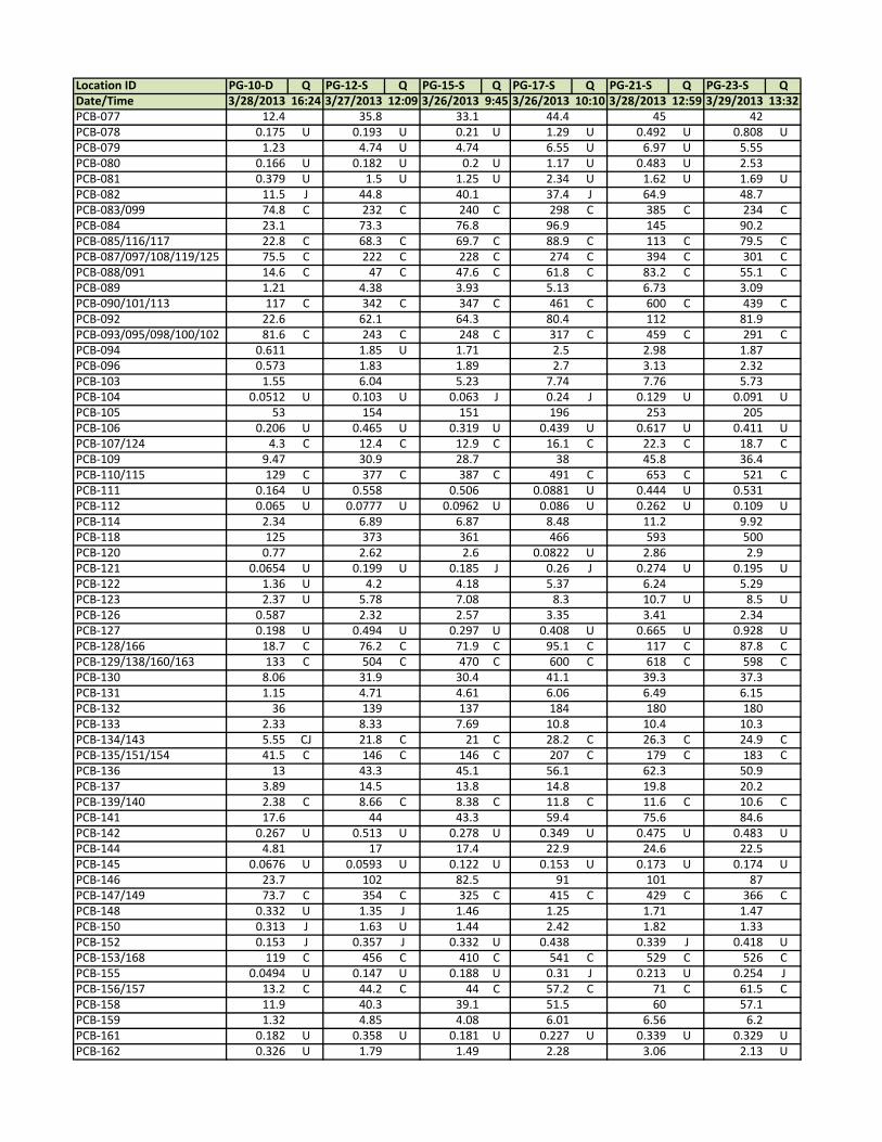
Location ID PG‐10‐D Q PG‐12‐S Q PG‐15‐S Q PG‐17‐S Q PG‐21‐S Q PG‐23‐S QDate/Time 3/28/2013 16:24 3/27/2013 12:09 3/26/2013 9:45 3/26/2013 10:10 3/28/2013 12:59 3/29/2013 13:32PCB‐077 12.4 35.8 33.1 44.4 45 42PCB‐078 0.175 U 0.193 U 0.21 U 1.29 U 0.492 U 0.808 UPCB‐079 1.23 4.74 U 4.74 6.55 U 6.97 U 5.55PCB‐080 0.166 U 0.182 U 0.2 U 1.17 U 0.483 U 2.53PCB‐081 0.379 U 1.5 U 1.25 U 2.34 U 1.62 U 1.69 UPCB‐082 11.5 J 44.8 40.1 37.4 J 64.9 48.7PCB‐083/099 74.8 C 232 C 240 C 298 C 385 C 234 CPCB‐084 23.1 73.3 76.8 96.9 145 90.2PCB‐085/116/117 22.8 C 68.3 C 69.7 C 88.9 C 113 C 79.5 CPCB‐087/097/108/119/125 75.5 C 222 C 228 C 274 C 394 C 301 CPCB‐088/091 14.6 C 47 C 47.6 C 61.8 C 83.2 C 55.1 CPCB‐089 1.21 4.38 3.93 5.13 6.73 3.09PCB‐090/101/113 117 C 342 C 347 C 461 C 600 C 439 CPCB‐092 22.6 62.1 64.3 80.4 112 81.9PCB‐093/095/098/100/102 81.6 C 243 C 248 C 317 C 459 C 291 CPCB‐094 0.611 1.85 U 1.71 2.5 2.98 1.87PCB‐096 0.573 1.83 1.89 2.7 3.13 2.32PCB‐103 1.55 6.04 5.23 7.74 7.76 5.73PCB‐104 0.0512 U 0.103 U 0.063 J 0.24 J 0.129 U 0.091 UPCB‐105 53 154 151 196 253 205PCB‐106 0.206 U 0.465 U 0.319 U 0.439 U 0.617 U 0.411 UPCB‐107/124 4.3 C 12.4 C 12.9 C 16.1 C 22.3 C 18.7 CPCB‐109 9.47 30.9 28.7 38 45.8 36.4PCB‐110/115 129 C 377 C 387 C 491 C 653 C 521 CPCB‐111 0.164 U 0.558 0.506 0.0881 U 0.444 U 0.531PCB‐112 0.065 U 0.0777 U 0.0962 U 0.086 U 0.262 U 0.109 UPCB‐114 2.34 6.89 6.87 8.48 11.2 9.92PCB‐118 125 373 361 466 593 500PCB‐120 0.77 2.62 2.6 0.0822 U 2.86 2.9PCB‐121 0.0654 U 0.199 U 0.185 J 0.26 J 0.274 U 0.195 UPCB‐122 1.36 U 4.2 4.18 5.37 6.24 5.29PCB‐123 2.37 U 5.78 7.08 8.3 10.7 U 8.5 UPCB‐126 0.587 2.32 2.57 3.35 3.41 2.34PCB‐127 0.198 U 0.494 U 0.297 U 0.408 U 0.665 U 0.928 UPCB‐128/166 18.7 C 76.2 C 71.9 C 95.1 C 117 C 87.8 CPCB‐129/138/160/163 133 C 504 C 470 C 600 C 618 C 598 CPCB‐130 8.06 31.9 30.4 41.1 39.3 37.3PCB‐131 1.15 4.71 4.61 6.06 6.49 6.15PCB‐132 36 139 137 184 180 180PCB‐133 2.33 8.33 7.69 10.8 10.4 10.3PCB‐134/143 5.55 CJ 21.8 C 21 C 28.2 C 26.3 C 24.9 CPCB‐135/151/154 41.5 C 146 C 146 C 207 C 179 C 183 CPCB‐136 13 43.3 45.1 56.1 62.3 50.9PCB‐137 3.89 14.5 13.8 14.8 19.8 20.2PCB‐139/140 2.38 C 8.66 C 8.38 C 11.8 C 11.6 C 10.6 CPCB‐141 17.6 44 43.3 59.4 75.6 84.6PCB‐142 0.267 U 0.513 U 0.278 U 0.349 U 0.475 U 0.483 UPCB‐144 4.81 17 17.4 22.9 24.6 22.5PCB‐145 0.0676 U 0.0593 U 0.122 U 0.153 U 0.173 U 0.174 UPCB‐146 23.7 102 82.5 91 101 87PCB‐147/149 73.7 C 354 C 325 C 415 C 429 C 366 CPCB‐148 0.332 U 1.35 J 1.46 1.25 1.71 1.47PCB‐150 0.313 J 1.63 U 1.44 2.42 1.82 1.33PCB‐152 0.153 J 0.357 J 0.332 U 0.438 0.339 J 0.418 UPCB‐153/168 119 C 456 C 410 C 541 C 529 C 526 CPCB‐155 0.0494 U 0.147 U 0.188 U 0.31 J 0.213 U 0.254 JPCB‐156/157 13.2 C 44.2 C 44 C 57.2 C 71 C 61.5 CPCB‐158 11.9 40.3 39.1 51.5 60 57.1PCB‐159 1.32 4.85 4.08 6.01 6.56 6.2PCB‐161 0.182 U 0.358 U 0.181 U 0.227 U 0.339 U 0.329 UPCB‐162 0.326 U 1.79 1.49 2.28 3.06 2.13 U

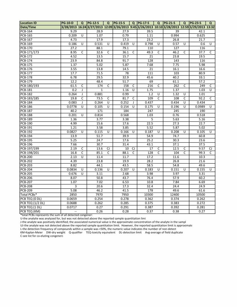
Location ID PG‐10‐D Q PG‐12‐S Q PG‐15‐S Q PG‐17‐S Q PG‐21‐S Q PG‐23‐S QDate/Time 3/28/2013 16:24 3/27/2013 12:09 3/26/2013 9:45 3/26/2013 10:10 3/28/2013 12:59 3/29/2013 13:32PCB‐164 9.29 28.9 27.9 39.5 39 42.1PCB‐165 0.209 U 1.07 0.79 1.11 0.994 0.625PCB‐167 4.73 17.9 17.3 23.2 26.8 21.7PCB‐169 0.186 U 0.531 U 0.419 U 0.798 U 0.57 U 0.6 UPCB‐170 27.2 88.1 79.1 110 127 116PCB‐171/173 8.95 C 32.6 C 36.1 C 49.3 C 46.2 C 37.7 CPCB‐172 4.52 13.5 15.7 21 23.8 19.5PCB‐174 23.9 84.8 91.7 128 143 116PCB‐175 1.37 5.02 5.87 7.68 7.75 5.98PCB‐176 3.55 13.8 14.5 21 16.1 16.6PCB‐177 17.7 71.5 78 111 103 80.9PCB‐178 6.78 29.5 32.9 45.6 40.2 33.1PCB‐179 12.2 48.4 51.7 69 61.1 57.2PCB‐180/193 61.5 C 174 C 158 C 216 C 262 C 249 CPCB‐181 0.2 J 1 1.16 U 1.75 1.37 1.03 UPCB‐182 0.264 J 0.881 0.99 1.2 U 1.32 U 1.01PCB‐183/185 19.8 C 73.5 C 81.7 C 109 C 108 C 92.2 CPCB‐184 0.083 J 0.264 U 0.252 J 0.437 0.434 U 0.434PCB‐186 0.0778 U 0.105 U 0.154 U 0.175 U 0.196 U 0.0989 UPCB‐187 40.2 171 184 247 245 190PCB‐188 0.201 U 0.814 0.568 1.03 0.76 0.518PCB‐189 1.36 3.77 3.38 5 5.63 5.16PCB‐190 4.99 15.6 17.6 22.5 27.3 22.7PCB‐191 1.21 3.58 3.85 5.52 5.87 5.02PCB‐192 0.0827 U 0.115 U 0.166 U 0.187 U 0.208 U 0.105 UPCB‐194 13.9 51.7 39.9 54.9 74.7 60.8PCB‐195 5.25 24.7 17.6 25.2 30.3 23.6PCB‐196 7.66 30.7 31.4 43.1 37.1 37.5PCB‐197/199 2.19 C 13.6 CJ 10 CJ 17 C 12.5 C 9.57 CJPCB‐198/201 16.8 C 85.1 C 88.1 C 128 C 104 C 99.3 CPCB‐200 2.13 U 11.4 11.7 17.2 11.6 10.3PCB‐202 4.39 23.8 19.9 28.2 26.8 21.6PCB‐203 8.82 44.1 43.5 58.5 54.8 49.6PCB‐204 0.0834 U 0.136 U 0.207 U 0.183 U 0.151 U 0.155 UPCB‐205 0.676 U 3.11 2.68 3.98 3.97 3.31PCB‐206 8.07 50.8 43.7 76.4 57.9 60.2PCB‐207 1.07 7.02 6.53 10.8 7.84 6.69PCB‐208 3 20.6 17.3 32.4 24.4 24.9PCB‐209 5.08 46.2 41.5 178 49.6 61.6Total PCBs* 2850 7970 7950 10300 12400 10500PCB TEQ (0 DL) 0.0659 0.254 0.278 0.362 0.374 0.262PCB TEQ (1/2 DL) 0.0688 0.262 0.285 0.375 0.383 0.272PCB TEQ (1 DL) 0.0717 0.27 0.291 0.387 0.392 0.281PCB TEQ (KM) ‐‐ 0.26 0.28 0.37 0.38 0.27*total PCBs represents the sum of all detected congenersU‐the analytie was analyzed for, but was not detected above the reported sample quantitation limiJ‐the analyte was positively identified; the associated numerical value is the approximate concentration of the analyte in the samplUJ‐the analyte was not detected above the reported sample quantitation limit. However, the reported quantitation limit is approximateL‐the detection frequency of compounds within a sample was <50%, the numeric value indicates the number of non‐detectKM‐Kaplan‐Meier DW‐dry weight Q‐qualifier TEQ‐toxicity equivalent DL‐detection limit Avg‐average of field duplicatesC‐see list for co‐eluting congeners

Table E‐3. Summary of Phase II Polychlorinated Biphenyl (PCB) Congener Data (continued).Location ID PG‐27‐S Q PG‐28‐S Q PG‐31‐S Q PG‐34‐S Q PG‐51‐S Q PG‐53‐S QDate/Time 3/28/2013 14:50 3/28/2013 19:36 3/27/2013 14:15 3/26/2013 10:39 4/22/2014 15:21 4/22/2014 9:58PCB Congeners (ng/kg DW)PCB‐001 16.3 1.48 6.42 21.2 7.75 J 12.7PCB‐002 18.8 13.2 10.9 22.7 12.9 9.67PCB‐003 17.1 2.29 5.38 13.9 4.86 J 22.6PCB‐004 25.1 2.17 8.28 26.7 13.8 18.7PCB‐005 0.954 0.212 U 0.259 J 0.829 2.3 U 1.74PCB‐006 10.4 1.33 2.5 10.4 3.74 J 12.1PCB‐007 4.01 0.25 J 1.36 4.67 2.18 U 3.53PCB‐008 71.4 7.55 18.3 74.1 32.8 63.9PCB‐009 2.66 0.367 J 0.666 2.54 2 U 3.23PCB‐010 1.18 0.19 U 0.355 J 1.06 1.89 U 1.07PCB‐011 32.1 13.3 11.2 36 21.3 26.2PCB‐012/013 11.4 C 2.99 C 8.22 CU 10.3 C 10.9 CU 9.33 CPCB‐014 0.986 U 0.188 U 0.405 U 0.91 U 2.2 U 0.617PCB‐015 72.9 13 20.6 81.1 36.3 54.4PCB‐016 29 4.75 5.13 24.5 11.7 48.4PCB‐017 47.7 5.8 9.38 42.1 18 59.1PCB‐018/030 72.2 C 9.95 C 11.4 C 52.4 C 25.6 C 130 CPCB‐019 8.02 1.36 2.95 7.57 3.71 9.46PCB‐020/028 234 C 41.6 C 57.9 C 245 C 117 C 294 CPCB‐021/033 68.9 C 14.1 C 15.3 C 67.2 C 28.4 C 118 CPCB‐022 56.5 11.8 12.3 53.5 24 91.8PCB‐023 0.397 U 0.141 U 0.938 0.224 U 0.113 U 0.24 JPCB‐024 0.794 0.134 U 0.159 J 0.831 0.6 U 1.5PCB‐025 14.4 2.13 3.57 15.5 7.02 16.4PCB‐026/029 26.5 C 4.39 C 6.55 C 28.3 C 13.8 C 36.3 CPCB‐027 7.84 0.961 J 2.13 6.88 4.92 J 10.2PCB‐031 149 28.7 34 142 66.4 236PCB‐032 43.8 4.43 10.6 41.5 26.8 49.1PCB‐034 0.981 0.208 U 1.01 1.15 0.452 0.971PCB‐035 6.36 1.31 1.97 7.19 4.26 5.38PCB‐036 1.21 0.344 J 0.523 1.9 0.912 0.753PCB‐037 86.7 16.2 22.5 93.4 44.7 69.2PCB‐038 0.609 0.133 U 0.352 U 0.672 0.377 J 0.552PCB‐039 1.55 0.26 J 0.434 1.63 0.905 2.66PCB‐040/041/071 102 C 15.9 C 25.1 C 109 C 54.2 C 157 CPCB‐042 56.8 9.1 13.9 57.9 28.1 74.5PCB‐043 5.45 1.22 1.41 6.74 2.81 10.7PCB‐044/047/065 215 C 32.3 C 50.8 C 202 C 104 C 305 CPCB‐045/051 25.9 C 3.64 C 6.64 C 27.9 C 12.9 C 37.3 CPCB‐046 8.04 1.29 U 2.18 9.14 4.45 12.5PCB‐048 33 5.5 7.58 33.6 14 55.4PCB‐049/069 155 C 21.8 C 38.3 C 150 C 72.2 C 193 CPCB‐050/053 24.2 C 3.08 C 5.56 C 23.3 C 11.5 C 30.4 CPCB‐052 256 33.3 52.5 208 104 449PCB‐054 0.307 J 0.121 U 0.64 0.444 0.207 J 0.337 JPCB‐055 4.13 0.549 0.749 3.33 1.74 4.9PCB‐056 113 22.5 27.1 104 57.3 168PCB‐057 1.14 0.211 U 0.342 J 1.22 0.484 0.415 UPCB‐058 1.35 0.219 U 0.279 U 1.34 0.546 0.443 UPCB‐059/062/075 18.5 C 2.79 C 4.57 C 20.2 C 10.1 C 24 CPCB‐060 60.9 10.6 14.5 55.5 31 95.7PCB‐061/070/074/076 479 C 85.6 C 110 C 429 C 218 C 665 CPCB‐063 11.1 1.74 2.69 10.9 5.12 12.6PCB‐064 92.4 14.4 20.8 85 41.3 144PCB‐066 270 53.8 70.3 265 137 307PCB‐067 8 1.33 2.22 9.23 3.96 9.23PCB‐068 2.22 0.444 0.783 2.92 1.46 1.65PCB‐072 3.56 0.553 1.09 4.27 2.25 3.02PCB‐073 0.715 U 0.115 J 0.192 U 1.05 0.0506 U 0.0979 U

Location ID PG‐27‐S LQ PG‐28‐S LQ PG‐31‐S LQ PG‐34‐S LQ PG‐51‐S Q PG‐53‐S QDate/Time 3/28/2013 14:50 3/28/2013 19:36 3/27/2013 14:15 3/26/2013 10:39 4/22/2014 15:21 4/22/2014 9:58PCB‐077 39.1 6.59 11.4 43 24.9 27.8PCB‐078 0.575 U 0.212 U 0.27 U 0.247 U 0.0981 U 0.458 UPCB‐079 6.04 0.707 1.51 5.82 3.17 15.8PCB‐080 0.534 U 0.196 U 0.249 U 0.234 U 0.0899 U 0.421 UPCB‐081 1.62 U 0.21 U 0.537 U 1.55 U 0.87 1.16PCB‐082 47.6 6.92 8.59 J 39.4 35.3 59.2PCB‐083/099 286 C 34.2 C 68.1 C 283 C 166 C 290 CPCB‐084 92.2 9.47 19.5 81.7 43.6 132PCB‐085/116/117 84.9 C 9.86 C 19.4 C 79.8 C 46.5 C 75.5 CPCB‐087/097/108/119/125 284 C 31.8 C 60.4 C 257 C 145 C 409 CPCB‐088/091 57.6 C 5.98 C 14 C 54.6 C 29.4 C 60.7 CPCB‐089 4.23 0.385 J 1.19 4.75 2.68 5.65PCB‐090/101/113 453 C 49 C 101 C 396 C 204 C 1400 CPCB‐092 80.8 9.41 18.9 71.4 40.7 196PCB‐093/095/098/100/102 319 C 34.9 C 68.3 C 270 C 141 C 1250 CPCB‐094 1.8 0.207 U 0.549 2.06 0.923 1.87PCB‐096 2.09 0.269 U 0.628 2.22 1.16 2.2PCB‐103 5.62 0.838 1.84 6.31 3.34 6.56PCB‐104 0.259 U 0.118 U 0.268 U 0.145 U 0.064 J 0.0776 UPCB‐105 202 23.9 48.7 196 111 181PCB‐106 1.08 U 0.279 U 0.348 U 0.449 U 0.302 U 0.75 UPCB‐107/124 17.1 C 1.64 C 3.88 C 16.2 C 9.23 C 16.6 CPCB‐109 35.6 4.5 9.41 39.4 22.6 33PCB‐110/115 502 C 58.2 C 115 C 449 C 248 C 884 CPCB‐111 0.535 U 0.141 U 0.175 U 0.598 0.356 U 0.388 UPCB‐112 0.433 U 0.14 U 0.129 U 0.182 U 0.0744 U 0.162 UPCB‐114 9.19 1.05 2.21 8.47 4.65 10PCB‐118 480 58.8 117 467 270 508PCB‐120 2.76 0.388 J 0.842 3.19 1.88 2.04 UPCB‐121 0.424 U 0.141 U 0.13 U 0.262 U 0.105 U 0.161 UPCB‐122 5.1 0.498 1.07 5.44 3.35 5.59PCB‐123 10.2 0.97 2.67 7.87 5.2 7.34PCB‐126 2.98 0.31 U 1.01 2.85 1.44 1.27 UPCB‐127 1.1 U 0.271 U 0.393 U 0.974 U 0.312 U 0.763 UPCB‐128/166 91.7 C 7.18 C 24.9 C 101 C 69.3 C 186 CPCB‐129/138/160/163 584 C 60.7 C 156 C 637 C 440 C 2150 CPCB‐130 36.6 3.23 9.6 40.6 24.5 73.7PCB‐131 6.5 0.497 1.41 5.65 U 4.05 13.5PCB‐132 173 15.8 41.5 173 110 728PCB‐133 9.58 1.03 2.87 11 6.21 23.4PCB‐134/143 26.3 C 2.17 CU 6.14 C 26.4 C 15.7 C 86 CPCB‐135/151/154 168 C 19.7 C 43.2 C 181 C 102 C 1070 CPCB‐136 50 5.78 12.8 55.9 30.8 405PCB‐137 19 1.65 U 4.5 17.2 12.4 13.4PCB‐139/140 10.2 C 0.92 C 2.74 C 11 C 7.36 C 7.8 CPCB‐141 69.4 8.81 13.9 58.9 35.1 569PCB‐142 1.01 U 0.299 U 0.332 U 0.794 U 0.494 U 1.73 UPCB‐144 19.8 2.37 5.27 21.7 13.5 161PCB‐145 0.349 U 0.169 U 0.142 U 0.171 J 0.12 J 0.0977 UPCB‐146 94.1 11.7 26.6 107 67.5 302PCB‐147/149 403 C 43.3 C 104 C 426 C 291 C 2330 CPCB‐148 1.74 0.211 U 0.34 J 1.52 1.34 U 1.32PCB‐150 1.61 0.168 U 0.59 1.83 0.878 0.955PCB‐152 0.316 J 0.153 U 0.128 U 0.474 0.198 J 0.357 JPCB‐153/168 506 C 53.9 C 141 C 574 C 352 C 2030 CPCB‐155 0.255 U 0.126 U 0.323 U 0.247 J 0.093 J 0.0716 UPCB‐156/157 58.1 C 5.85 C 14.4 C 59.7 C 35.4 C 120 CPCB‐158 51.9 5.04 12.8 53 31.1 176PCB‐159 4.37 U 0.477 1.25 5.5 0.328 U 1.22 UPCB‐161 0.73 U 0.204 U 0.226 U 0.535 U 0.337 U 1.24 UPCB‐162 0.728 U 0.213 U 0.463 U 2.14 0.332 U 1.27 U

Location ID PG‐27‐S LQ PG‐28‐S LQ PG‐31‐S LQ PG‐34‐S LQ PG‐51‐S Q PG‐53‐S QDate/Time 3/28/2013 14:50 3/28/2013 19:36 3/27/2013 14:15 3/26/2013 10:39 4/22/2014 15:21 4/22/2014 9:58PCB‐164 36.7 3.92 8.99 38.6 22.3 168PCB‐165 0.811 U 0.235 U 0.343 U 1.47 U 0.588 U 1.4 UPCB‐167 21.6 2.13 5.8 23.5 14 44PCB‐169 0.74 U 0.207 U 0.233 U 0.634 U 0.31 U 3.17 UPCB‐170 109 12 28.7 122 57.8 623PCB‐171/173 42.8 C 4.06 C 12.2 C 49.3 C 23.1 C 222 CPCB‐172 21.2 2.15 5.45 21.8 10.2 123PCB‐174 117 12.6 34.1 136 66.9 873PCB‐175 6.09 0.585 U 1.96 7.76 3.46 31.5PCB‐176 16.8 1.81 4.75 20.9 10.1 103PCB‐177 83.1 8.76 27.2 110 53.9 465PCB‐178 33.4 2.93 11.1 44.2 20.8 154PCB‐179 55.6 5.37 17.3 71.3 36 346PCB‐180/193 222 C 26.9 C 60.7 C 236 C 112 C 1400 CPCB‐181 0.983 0.191 U 0.281 U 1.6 0.872 2.07PCB‐182 1.05 0.181 U 0.436 U 1.41 0.583 0.231 UPCB‐183/185 92.3 C 8.86 C 26.7 C 110 C 48.2 C 507 CPCB‐184 0.417 U 0.134 U 0.164 U 0.423 0.246 U 0.175 UPCB‐186 0.454 U 0.147 U 0.179 U 0.195 U 0.182 U 0.187 UPCB‐187 200 18.1 64.2 255 153 1030PCB‐188 0.802 0.13 U 0.267 J 0.964 0.434 0.229 UPCB‐189 5.3 0.518 1.5 5.5 2.32 19.1PCB‐190 21.8 2.49 5.96 25.2 10.8 129PCB‐191 5.12 0.426 1.48 5.54 2.12 29.2PCB‐192 0.492 U 0.167 U 0.204 U 0.213 U 0.189 U 0.201 UPCB‐194 58.9 5.17 17.8 63.7 29.2 239PCB‐195 23.4 2.13 U 6.85 31.4 13.7 105PCB‐196 33.3 2.78 11.1 46.3 18 137PCB‐197/199 12 C 0.988 C 3.64 C 16.9 C 8.41 C 43.9 CJPCB‐198/201 96.5 C 6.67 C 31.3 C 133 C 45.2 C 266 CPCB‐200 12.1 0.829 4.17 16.7 7.65 34PCB‐202 21.8 1.36 7.38 30 14.2 46.3PCB‐203 51.4 3.77 15.7 66.6 30.6 164PCB‐204 0.31 U 0.155 U 0.147 U 0.226 J 0.14 U 0.147 UPCB‐205 2.76 0.375 J 1.08 3.94 1.66 11.3PCB‐206 47.7 2.35 17 67.4 30.4 44.8PCB‐207 6.47 0.354 J 2.16 9.2 4.24 7.07PCB‐208 19.2 0.828 6.62 27.9 12.8 12.4PCB‐209 37.7 1.55 16.1 67.6 28.8 10.7Total PCBs* 10000 1260 2530 10200 5550 27600PCB TEQ (0 DL) 0.326 0.00346 0.108 0.312 0.16 0.0298PCB TEQ (1/2 DL) 0.337 0.0221 0.111 0.322 0.162 0.141PCB TEQ (1 DL) 0.348 0.0407 0.115 0.332 0.167 0.252PCB TEQ (KM) 0.33 0.035 L 0.11 0.32 0.16 0.16 L*total PCBs represents the sum of all detected congenersU‐the analytie was analyzed for, but was not detected above the reported sample quantitation limiJ‐the analyte was positively identified; the associated numerical value is the approximate concentration of the analyte in the samplUJ‐the analyte was not detected above the reported sample quantitation limit. However, the reported quantitation limit is approximateL‐the detection frequency of compounds within a sample was <50%, the numeric value indicates the number of non‐detectKM‐Kaplan‐Meier DW‐dry weight Q‐qualifier TEQ‐toxicity equivalent DL‐detection limit Avg‐average of field duplicatesC‐see list for co‐eluting congeners

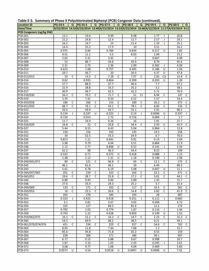
Table E‐3. Summary of Phase II Polychlorinated Biphenyl (PCB) Congener Data (continued).Location ID PG‐54‐S Q PG‐55‐S Q PG‐57‐S Q PG‐58‐S Q PG‐59‐S Q PG‐60‐S QDate/Time 4/22/2014 14:10 4/23/2014 12:40 4/22/2014 13:23 4/22/2014 10:46 4/22/2014 11:17 4/23/2014 9:11PCB Congeners (ng/kg DW)PCB‐001 12.1 19.4 9.49 9.48 1.77 J 20.8PCB‐002 21.2 24.8 12.4 11.7 2.57 J 24.1PCB‐003 16.1 14.7 15 11.4 1.33 J 25.1PCB‐004 14.4 25.2 17.9 10 3.51 34.2PCB‐005 0.975 0.84 0.784 0.834 0.217 U 1.82PCB‐006 9.51 11.1 5.5 8.03 1.04 15.2PCB‐007 2.65 5.31 3.42 2 0.667 4.98PCB‐008 52 86.7 34.6 43.9 8.79 95.6PCB‐009 2.31 2.73 2.36 2.09 0.302 J 4.09PCB‐010 0.623 1.08 0.757 0.495 0.186 U 1.56PCB‐011 29.7 46.7 20 20.4 4.37 U 47.8PCB‐012/013 10 C 14.5 C 7.28 C 7.07 C 2.05 CU 15.8 CPCB‐014 0.62 0.933 0.804 0.399 0.203 U 1.28PCB‐015 57.7 88.9 37.7 40.4 7.7 97.2PCB‐016 22.9 28.8 33.3 25.2 3.2 58.1PCB‐017 30.9 46.7 42.5 31.3 5.71 76.9PCB‐018/030 56.3 C 70.2 C 71.7 C 51 CJ 8.94 C 147 CPCB‐019 5.35 7.41 9.33 4.52 1.57 14.4PCB‐020/028 186 C 266 C 155 C 180 C 26.2 C 372 CPCB‐021/033 66.7 C 76.1 C 54.1 C 78.1 C 6.82 C 126 CPCB‐022 50.5 59.9 43.7 55.1 5.91 96.2PCB‐023 0.134 J 0.247 U 0.322 J 0.14 J 0.0496 U 0.337 JPCB‐024 0.724 0.914 1.72 0.716 0.094 J 1.7PCB‐025 11.7 16.9 9.26 16 1.91 21.7PCB‐026/029 24.8 C 32 C 20.8 C 34.4 C 2.93 C 45.9 CPCB‐027 5.44 9.15 6.43 5.04 0.964 J 12.8PCB‐031 136 156 105 135 14.5 258PCB‐032 30 52.5 33.3 24.9 6.7 76.6PCB‐034 0.813 1.11 0.441 0.91 0.13 J 1.64PCB‐035 5.98 9.79 4.64 3.51 0.864 11.9PCB‐036 1.12 1.77 0.848 U 0.52 0.145 J 2.04PCB‐037 61.2 98 46.3 54.4 8.22 109PCB‐038 0.532 0.71 0.372 U 0.418 0.088 J 1.13PCB‐039 1.48 2.12 1.31 U 1.18 0.198 J 2.98PCB‐040/041/071 89 C 121 C 96.8 C 69 C 12.1 C 173 CPCB‐042 46.1 61.6 46.1 39 6.44 89.2PCB‐043 5.61 6.78 6.19 5.08 0.607 U 11.1PCB‐044/047/065 201 C 239 C 163 C 164 C 22.5 C 371 CPCB‐045/051 19.6 C 28.7 C 25.8 C 17.2 C 3.01 C 44.1 CPCB‐046 6.88 9.93 9.86 5.89 1.35 15.7PCB‐048 27.6 35.9 29.3 25.2 3.7 55.4PCB‐049/069 133 C 171 C 102 C 117 C 16.5 C 261 CPCB‐050/053 18 C 25.5 C 20.6 C 14.8 C 3.82 C 41.9 CPCB‐052 265 278 185 194 28 487PCB‐054 0.333 J 0.425 0.418 0.251 J 0.112 J 0.683PCB‐055 3.1 3.81 3.67 3.65 0.506 4.72PCB‐056 102 127 84.5 81.6 12.2 174PCB‐057 0.792 1.02 0.774 1.87 0.116 J 1.44PCB‐058 0.793 1.15 0.628 0.859 0.149 U 1.52PCB‐059/062/075 16.1 C 21.1 C 16.2 C 14.7 C 2.23 C 31.3 CPCB‐060 54.5 69.9 48.2 38.5 6.21 94.1PCB‐061/070/074/076 451 C 534 C 329 C 357 C 54.6 C 762 CPCB‐063 8.93 11.8 7.44 7.68 1.2 15.7PCB‐064 85.6 94.8 71.8 65.2 9.55 159PCB‐066 228 306 171 186 30.1 397PCB‐067 6.77 9.15 5.88 9.67 0.998 10.7PCB‐068 1.87 3.16 1.05 2.43 0.295 J 3.61PCB‐072 3.08 4.77 1.68 4.04 0.469 5.83PCB‐073 0.0573 U 4.54 0.0518 U 0.0497 U 0.0496 U 7.41

Location ID PG‐54‐S Q PG‐55‐S Q PG‐57‐S Q PG‐58‐S Q PG‐59‐S Q PG‐60‐S QDate/Time 4/22/2014 14:10 4/23/2014 12:40 4/22/2014 13:23 4/22/2014 10:46 4/22/2014 11:17 4/23/2014 9:11PCB‐077 29 48.4 24.6 19 5.53 48.3PCB‐078 0.258 U 0.407 U 0.145 U 0.146 U 0.0632 U 0.466 UPCB‐079 5.81 10.9 4.12 4.29 1.17 10.1PCB‐080 0.234 U 0.373 U 0.132 U 0.132 U 0.0573 U 0.427 UPCB‐081 1.2 1.85 1.08 0.71 0.188 J 2.08PCB‐082 51.9 J 78.2 49 29.2 J 6.94 94.7PCB‐083/099 266 C 375 C 164 C 173 C 37.8 C 437 CPCB‐084 94.5 124 64.9 57.4 12.3 149PCB‐085/116/117 76.3 C 108 C 55.6 C 43.2 C 9.53 C 128 CPCB‐087/097/108/119/125 294 C 375 C 197 C 167 C 35.1 C 449 CPCB‐088/091 55.8 C 76.5 C 35.4 C 36.3 C 7.23 C 85.3 CPCB‐089 4.2 7.01 3.93 2.82 0.565 6.58PCB‐090/101/113 432 C 568 C 253 C 242 C 50.2 C 704 CPCB‐092 82.3 103 44.1 54.6 9.75 136PCB‐093/095/098/100/102 315 C 415 C 195 C 180 C 41.8 C 514 CPCB‐094 1.75 1.79 J 1.19 J 1.14 0.246 U 2.72 JPCB‐096 1.9 2.85 J 1.52 J 1.34 0.235 J 2.99 JPCB‐103 4.14 7.35 2.24 J 3.16 0.768 8.39PCB‐104 0.0609 U 0.131 J 0.0507 U 0.0497 U 0.0496 U 0.12 UPCB‐105 181 249 124 100 22.5 262PCB‐106 0.467 U 1.08 U 0.644 U 0.364 U 0.0909 U 1.02 UPCB‐107/124 16.6 C 22.6 C 11.1 C 8.17 C 2.1 C 25.6 CPCB‐109 32.6 51.1 22.6 20.2 4.45 58PCB‐110/115 480 C 642 C 341 C 291 C 60.4 C 802 CPCB‐111 0.293 J 0.607 U 0.314 U 0.316 U 0.097 U 0.927 JPCB‐112 0.117 U 0.606 U 0.299 U 0.113 U 0.0496 U 0.57 UPCB‐114 8.28 11.3 6.15 5.11 0.937 13.6PCB‐118 440 632 283 262 58.9 712PCB‐120 1.48 3.53 J 0.683 U 1.18 0.334 U 3.67 JPCB‐121 0.121 U 0.606 U 0.297 U 0.116 U 0.0496 U 0.566 UPCB‐122 5.5 7.26 3.59 J 2.87 0.708 8.27PCB‐123 8.15 10.1 5.48 3.6 1.13 12.4PCB‐126 1.4 2.46 1.43 U 0.838 0.495 3.2PCB‐127 0.479 U 1.14 U 0.693 U 0.373 U 0.0933 U 1.09 UPCB‐128/166 108 C 156 C 64.2 C 59.2 C 12.8 C 173 CPCB‐129/138/160/163 708 C 911 C 443 C 400 C 80 C 1040 CPCB‐130 38.8 56.4 27.2 21.2 4.43 60.5PCB‐131 7.71 9.47 3.93 3.87 0.894 11.3PCB‐132 203 249 117 118 19.8 325PCB‐133 7.6 12.7 3.53 J 4.78 1.03 U 15.4PCB‐134/143 27.9 C 38.9 C 18.2 C 16.3 C 2.93 C 48.8 CPCB‐135/151/154 178 C 217 C 99.9 C 109 C 17.3 C 286 CPCB‐136 61.5 75.1 30.1 36.2 5.99 92.8PCB‐137 28 30.1 18.7 15.6 3.13 44.1PCB‐139/140 10.2 C 15.3 C 6.05 C 6.78 C 1.31 C 17.8 CPCB‐141 83 84.3 50.9 49.2 7.76 133PCB‐142 0.421 U 0.588 U 0.941 U 0.562 U 0.212 U 1.18 UPCB‐144 27 30.1 13.6 14.1 2.28 42.3PCB‐145 0.167 J 0.376 J 0.411 U 0.0873 U 0.0576 U 0.371 JPCB‐146 83.3 133 38.1 49.6 10.7 160PCB‐147/149 534 C 595 C 296 C 332 C 53 C 783 CPCB‐148 1.27 J 2.43 0.522 U 0.883 0.138 J 2.29PCB‐150 1.16 1.83 0.639 J 1.01 0.126 J 1.96PCB‐152 0.446 0.511 U 0.365 U 0.353 J 0.0513 U 0.737PCB‐153/168 464 C 740 C 235 C 241 C 55.9 C 856 CPCB‐155 0.175 J 0.212 J 0.108 U 0.109 U 0.0496 U 0.174 JPCB‐156/157 59.4 C 86.6 C 26.5 C 30.2 C 6.56 C 102 CPCB‐158 56.9 74.4 38 31.4 5.91 91.5PCB‐159 0.29 U 0.391 U 2.03 J 0.387 U 0.146 U 0.785 UPCB‐161 0.293 U 0.401 U 0.656 U 0.392 U 0.148 U 0.805 UPCB‐162 0.296 U 0.396 U 0.684 U 0.395 U 0.149 U 0.795 U

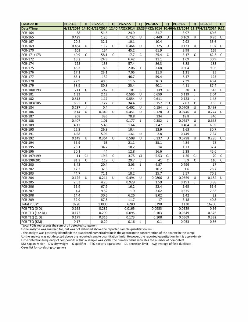
Location ID PG‐54‐S Q PG‐55‐S Q PG‐57‐S Q PG‐58‐S Q PG‐59‐S Q PG‐60‐S QDate/Time 4/22/2014 14:10 4/23/2014 12:40 4/22/2014 13:23 4/22/2014 10:46 4/22/2014 11:17 4/23/2014 9:11PCB‐164 38 51.5 24.9 21.7 3.97 60.6PCB‐165 0.429 1.23 0.732 U 0.449 U 0.169 U 0.93 UPCB‐167 20.2 32.1 10.1 10.4 2.92 35.6PCB‐169 0.484 U 1.12 U 0.464 U 0.325 U 0.133 U 1.07 UPCB‐170 103 134 45.2 61.9 9.98 169PCB‐171/173 40.9 C 58.1 C 17.7 C 25.4 C 3.17 C 62.5 CPCB‐172 18.2 24.9 6.42 11.1 1.69 30.9PCB‐174 125 153 57.4 86.3 8.88 183PCB‐175 4.93 8.6 2.06 J 2.68 0.504 9.05PCB‐176 17.1 23.1 7.05 11.3 1.21 25PCB‐177 85.1 132 46.7 59.4 6.47 125PCB‐178 27.9 49.5 11.6 16.3 2.39 48.4PCB‐179 58.9 80.3 25.4 40.1 4.11 87.4PCB‐180/193 211 C 247 C 101 C 139 C 20 C 345 CPCB‐181 1.33 2.13 0.595 U 0.659 0.119 J 2.04PCB‐182 0.813 1.17 0.554 U 0.611 0.123 J 1.48PCB‐183/185 85.5 C 122 C 34.4 C 0.157 CU 7.07 C 135 CPCB‐184 0.237 J 0.4 0.402 U 0.154 J 0.0709 U 0.498PCB‐186 0.14 U 0.349 U 0.451 U 0.128 U 0.0746 U 0.274 UPCB‐187 208 335 78.8 134 18.8 340PCB‐188 0.407 1.01 0.177 J 0.352 J 0.0657 U 0.653PCB‐189 4.12 5.46 1.64 2.47 0.404 U 6.59PCB‐190 22.9 26.9 10.4 13.9 1.63 30.7PCB‐191 4.68 5.95 1.61 U 2.8 0.449 7.34PCB‐192 0.149 U 0.364 U 0.508 U 0.137 U 0.0798 U 0.285 UPCB‐194 53.9 68 21.1 35.1 4.84 78PCB‐195 23.1 34.7 10.2 14 1.73 32.4PCB‐196 30.1 44 12.8 16.6 2.38 45.6PCB‐197/199 11 CJ 19.6 C 3.75 CJ 5.53 CJ 1.26 CJ 20 CPCB‐198/201 81.2 C 119 C 29.7 C 41 C 5.9 C 110 CPCB‐200 8.43 20.4 3.03 J 4.87 0.796 17PCB‐202 17.2 32.3 7.1 10.2 1.6 28.7PCB‐203 44.7 71.1 18.2 25.7 3.57 70.3PCB‐204 0.125 U 0.214 U 0.494 U 0.0806 U 0.0659 U 0.182 UPCB‐205 2.53 4.25 0.929 1.59 0.193 J 3.88PCB‐206 33.9 67.9 16.2 22.4 3.65 53.6PCB‐207 4.4 9.52 1.9 2.62 0.575 7.63PCB‐208 14.4 30.6 6.26 8.02 1.42 22PCB‐209 32.9 87.8 11.7 17 3.18 40.8Total PCBs* 9720 13000 6280 6390 1130 16200PCB TEQ (0 DL) 0.165 0.282 0.0165 0.0983 0.0529 0.36PCB TEQ (1/2 DL) 0.172 0.299 0.095 0.103 0.0549 0.376PCB TEQ (1 DL) 0.179 0.316 0.173 0.108 0.0569 0.392PCB TEQ (KM) 0.17 0.29 0.16 L 0.1 0.053 0.36*total PCBs represents the sum of all detected congenersU‐the analytie was analyzed for, but was not detected above the reported sample quantitation limiJ‐the analyte was positively identified; the associated numerical value is the approximate concentration of the analyte in the samplUJ‐the analyte was not detected above the reported sample quantitation limit. However, the reported quantitation limit is approximateL‐the detection frequency of compounds within a sample was <50%, the numeric value indicates the number of non‐detectKM‐Kaplan‐Meier DW‐dry weight Q‐qualifier TEQ‐toxicity equivalent DL‐detection limit Avg‐average of field duplicatesC‐see list for co‐eluting congeners

Table E‐3. Summary of Phase II Polychlorinated Biphenyl (PCB) Congener Data (continued).Location ID PG‐61‐S Q PG‐62‐S Q PG‐64‐S Q PG‐65‐S Q PG‐65‐D Q PT‐03‐S QDate/Time 4/23/2014 13:13 4/22/2014 13:46 4/22/2014 12:03 4/23/2014 11:08 4/23/2014 11:08 5/10/2013 13:07PCB Congeners (ng/kg DW)PCB‐001 13.7 6.4 4.4 13.8 7.44 6.3PCB‐002 21.7 11.1 4.37 17.3 9.64 25.1PCB‐003 10.1 9.7 3.65 J 16.9 10.1 6.69PCB‐004 17.9 8.83 10.7 46.6 J 10.8 J 8.55PCB‐005 0.69 0.564 0.246 J 1.05 0.68 0.324 JPCB‐006 8.93 4.98 2.61 10.2 J 6.06 J 4.16PCB‐007 3.62 1.63 1.76 3.72 2.56 1.66PCB‐008 62.4 28.4 22.6 63.1 J 37.6 J 28.9PCB‐009 2.24 1.35 0.763 2.67 1.57 1.11PCB‐010 0.849 0.398 0.616 1.38 0.597 0.441PCB‐011 30.7 19.5 8.14 30.9 19.6 57.2PCB‐012/013 8.22 C 6.07 C 3.46 CUJ 11 CUJ 5.9 CJ 6.04 CPCB‐014 0.64 0.844 U 0.255 J 0.843 0.493 0.699PCB‐015 53.2 33.1 16 51.1 34.9 37.9PCB‐016 19.7 16.5 9.14 33.3 20.7 7.69PCB‐017 31.9 19.5 17.7 46.1 31 11.2PCB‐018/030 47.1 C 38.4 C 24.5 C 90.7 CJ 51.7 CJ 15.8 CPCB‐019 5.09 3.62 5.67 10.3 J 4.64 J 1.85PCB‐020/028 172 C 116 C 57.9 C 211 C 144 C 87.9 CPCB‐021/033 52.6 C 42.1 C 16.3 C 72 C 49.7 C 27.5 CPCB‐022 39.3 32.5 13.5 55.7 38.1 19.7PCB‐023 0.171 U 0.122 U 0.071 U 0.24 U 0.127 U 0.152 UPCB‐024 0.671 0.474 0.335 J 1.08 0.575 0.221 JPCB‐025 10.9 7.35 4.48 12.6 8.52 6.03PCB‐026/029 20.7 C 15.8 C 7.21 C 26.7 C 17.5 C 9.93 CPCB‐027 5.11 3.44 3.2 J 8.49 4.64 2.01PCB‐031 105 88.4 35.1 149 101 50PCB‐032 34.1 18.7 23.4 38.1 25.5 11.8PCB‐034 0.848 0.497 0.233 J 0.913 0.623 0.304 JPCB‐035 5.48 3.97 1.81 5.78 3.48 4.13PCB‐036 1 0.768 0.267 U 0.82 0.5 2.47PCB‐037 55.2 36.4 16.7 59 38.9 32.4PCB‐038 0.467 0.335 J 0.192 J 0.581 0.361 J 0.335 JPCB‐039 1.37 0.979 0.567 1.83 1.17 0.693PCB‐040/041/071 73.3 C 54.8 C 42.5 C 96.8 C 64.4 C 32.3 CPCB‐042 37.5 28.4 21.1 50.2 33.6 14.8PCB‐043 4.67 3.52 2.35 6.08 4.27 1.41PCB‐044/047/065 166 C 121 C 77.7 C 194 C 129 C 56 CPCB‐045/051 17.3 C 12.2 C 11.9 C 23.7 C 16 C 5.79 CPCB‐046 5.8 4.37 5.09 8.03 5.39 2.23PCB‐048 22.1 17.7 11.9 31.9 22 8.3PCB‐049/069 111 C 81.8 C 53.8 C 139 C 91.8 C 37.6 CPCB‐050/053 16.2 C 11.7 C 14.3 C 21.1 C 14.2 C 5.86 CPCB‐052 228 154 91.8 227 150 57.9PCB‐054 0.287 J 0.196 J 0.484 0.407 J 0.216 J 0.13 JPCB‐055 1.96 2.34 1.03 3.08 J 1.83 J 1.02PCB‐056 82.2 64.1 32 104 76.5 35.8PCB‐057 0.502 0.548 0.321 J 0.93 0.489 0.374 JPCB‐058 0.736 0.564 0.345 J 1.01 0.595 0.272 JPCB‐059/062/075 12.9 C 10 C 8.02 C 17.3 C 11.3 C 5.02 CPCB‐060 42.6 36 16.6 54.6 39.6 20.3PCB‐061/070/074/076 371 C 295 C 141 C 430 C 285 C 137 CPCB‐063 7.13 5.82 3.11 8.8 6.15 3.2PCB‐064 64.7 51.9 30.8 83.6 56.7 21.8PCB‐066 195 147 77.4 230 162 83.1PCB‐067 5.3 4.19 2.89 6.71 4.26 2.69PCB‐068 1.79 1.18 0.768 1.99 1.32 0.942PCB‐072 2.87 1.99 1.31 3.27 J 1.91 J 1.21PCB‐073 0.0573 U 0.0645 U 0.0484 U 0.124 U 0.0738 U 0.0801 U

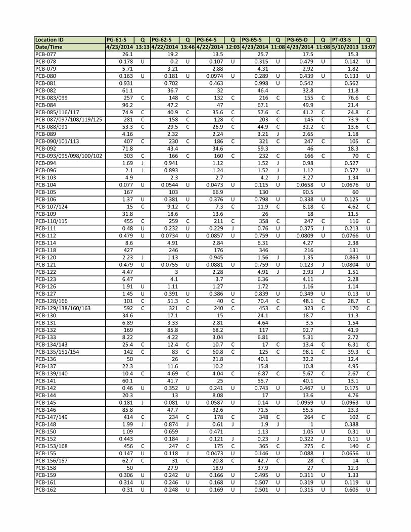
Location ID PG‐61‐S Q PG‐62‐S Q PG‐64‐S Q PG‐65‐S Q PG‐65‐D Q PT‐03‐S QDate/Time 4/23/2014 13:13 4/22/2014 13:46 4/22/2014 12:03 4/23/2014 11:08 4/23/2014 11:08 5/10/2013 13:07PCB‐077 26.1 19.2 13.5 25.7 17.5 15.3PCB‐078 0.178 U 0.2 U 0.107 U 0.315 U 0.479 U 0.142 UPCB‐079 5.71 3.21 2.88 4.31 2.92 1.82PCB‐080 0.163 U 0.181 U 0.0974 U 0.289 U 0.439 U 0.133 UPCB‐081 0.931 0.702 0.463 0.998 U 0.542 0.562PCB‐082 61.1 36.7 32 46.4 32.8 11.8PCB‐083/099 257 C 148 C 132 C 216 C 155 C 76.6 CPCB‐084 96.2 47.2 47 67.1 49.9 21.4PCB‐085/116/117 74.9 C 40.9 C 35.6 C 57.6 C 41.2 C 24.8 CPCB‐087/097/108/119/125 281 C 158 C 128 C 203 C 145 C 73.9 CPCB‐088/091 53.3 C 29.5 C 26.9 C 44.9 C 32.2 C 13.6 CPCB‐089 4.16 2.32 2.24 3.21 J 2.65 1.18PCB‐090/101/113 407 C 230 C 186 C 321 C 247 C 105 CPCB‐092 71.8 43.4 34.6 59.3 46 18.3PCB‐093/095/098/100/102 303 C 166 C 160 C 232 C 166 C 70 CPCB‐094 1.69 J 0.941 1.12 1.52 J 0.98 0.527PCB‐096 2.1 J 0.893 1.24 1.52 J 1.12 0.572 UPCB‐103 4.9 2.3 2.7 4.2 J 3.27 1.34PCB‐104 0.077 U 0.0544 U 0.0473 U 0.115 U 0.0658 U 0.0676 UPCB‐105 167 103 66.9 130 90.5 60PCB‐106 1.37 U 0.381 U 0.376 U 0.798 U 0.338 U 0.125 UPCB‐107/124 15 C 9.12 C 7.3 C 11.9 C 8.18 C 4.62 CPCB‐109 31.8 18.6 13.6 26 18 11.5PCB‐110/115 455 C 259 C 211 C 358 C 247 C 116 CPCB‐111 0.48 U 0.232 U 0.229 J 0.76 U 0.375 J 0.213 UPCB‐112 0.479 U 0.0734 U 0.0857 U 0.759 U 0.0809 U 0.0766 UPCB‐114 8.6 4.91 2.84 6.31 4.27 2.38PCB‐118 427 246 176 346 216 131PCB‐120 2.23 J 1.13 0.945 1.56 J 1.35 0.863 UPCB‐121 0.479 U 0.0755 U 0.0881 U 0.759 U 0.123 J 0.0804 UPCB‐122 4.47 3 2.28 4.91 J 2.93 J 1.51PCB‐123 6.47 4.1 3.7 6.36 4.11 2.28PCB‐126 1.91 U 1.11 1.27 1.72 1.16 1.14PCB‐127 1.45 U 0.391 U 0.386 U 0.839 U 0.349 U 0.13 UPCB‐128/166 101 C 51.3 C 40 C 70.4 C 48.1 C 28.7 CPCB‐129/138/160/163 592 C 321 C 240 C 453 C 323 C 170 CPCB‐130 34.6 17.1 15 24.1 18.7 11.3PCB‐131 6.89 3.33 2.81 4.64 3.5 1.54PCB‐132 169 85.8 68.2 117 92.7 41.9PCB‐133 8.22 4.22 3.04 6.81 5.31 2.72PCB‐134/143 25.4 C 12.4 C 10.7 C 17 C 13.4 C 6.31 CPCB‐135/151/154 142 C 83 C 60.8 C 125 C 98.1 C 39.3 CPCB‐136 50 26 21.8 40.1 32.2 12.4PCB‐137 22.3 11.6 10.2 15.8 10.8 4.95PCB‐139/140 10.4 C 4.69 C 4.04 C 6.87 C 5.67 C 2.67 CPCB‐141 60.1 41.7 25 55.7 40.1 13.1PCB‐142 0.46 U 0.352 U 0.241 U 0.743 U 0.467 U 0.175 UPCB‐144 20.3 13 8.08 17 13.6 4.76PCB‐145 0.181 J 0.081 U 0.0587 U 0.14 U 0.0959 U 0.0963 UPCB‐146 85.8 47.7 32.6 71.5 55.5 23.3PCB‐147/149 414 C 234 C 178 C 348 C 264 C 102 CPCB‐148 1.99 J 0.874 J 0.61 J 1.9 J 1 0.388PCB‐150 1.09 0.659 0.471 1.13 1.05 U 0.31 UPCB‐152 0.443 0.184 J 0.121 J 0.23 J 0.322 J 0.11 UPCB‐153/168 456 C 247 C 175 C 365 C 275 C 140 CPCB‐155 0.147 U 0.118 J 0.0473 U 0.146 U 0.088 J 0.0656 UPCB‐156/157 62.7 C 31 C 20.8 C 42.7 C 28 C 14 CPCB‐158 50 27.9 18.9 37.9 27 12.3PCB‐159 0.306 U 0.242 U 0.166 U 0.495 U 0.311 U 1.33PCB‐161 0.314 U 0.246 U 0.168 U 0.507 U 0.319 U 0.119 UPCB‐162 0.31 U 0.248 U 0.169 U 0.501 U 0.315 U 0.605 U

Location ID PG‐61‐S Q PG‐62‐S Q PG‐64‐S Q PG‐65‐S Q PG‐65‐D Q PT‐03‐S QDate/Time 4/23/2014 13:13 4/22/2014 13:46 4/22/2014 12:03 4/23/2014 11:08 4/23/2014 11:08 5/10/2013 13:07PCB‐164 32.4 18.1 13.5 26.6 19.6 8.7PCB‐165 0.61 U 0.296 J 0.192 U 0.586 U 0.368 U 0.276 JPCB‐167 21.2 11.3 8.77 15.6 9.72 5.85PCB‐169 0.279 U 0.367 U 0.139 U 0.593 U 0.429 U 0.195 UPCB‐170 87.1 74.6 29.7 75.5 52.3 24.5PCB‐171/173 37 C 24 C 9.76 C 27.8 CJ 14.9 CJ 10 CPCB‐172 15.7 13.6 5.28 15.3 J 8.62 J 3.97PCB‐174 93.1 82.3 30.3 84.5 J 47.1 J 24.5PCB‐175 4.84 3.68 1.53 4.06 2.48 1.68PCB‐176 13.3 9.64 3.89 10.8 6.93 3.82PCB‐177 77.3 50.9 23.5 54.7 J 32.8 J 23PCB‐178 27.2 18.8 8.79 21 13.2 10.2PCB‐179 46.1 33.9 14 37.4 25.4 13.8PCB‐180/193 156 C 171 C 61.5 C 163 C 116 C 48.7 CPCB‐181 1.37 0.735 0.32 J 0.755 0.466 U 0.231 JPCB‐182 0.912 0.641 U 0.341 J 0.705 0.45 0.343 JPCB‐183/185 71.6 C 59.2 C 23 C 63.4 CJ 35.7 CJ 21.4 CPCB‐184 0.278 J 0.24 J 0.0908 U 0.226 U 0.122 J 0.102 UPCB‐186 0.131 U 0.113 U 0.0956 U 0.218 U 0.123 U 0.103 UPCB‐187 196 141 59.3 167 J 92.3 J 54PCB‐188 0.507 U 0.283 J 0.162 J 0.335 U 0.265 U 0.194 JPCB‐189 3.69 2.82 1.14 2.99 2.09 1.06PCB‐190 17.9 15.5 4.99 14.4 J 7.26 J 4.43PCB‐191 4.11 3.13 1.17 3.12 J 1.71 J 0.871PCB‐192 0.137 U 0.121 U 0.102 U 0.227 U 0.128 U 0.114 UPCB‐194 38.2 65.7 14.5 43.3 31.2 13PCB‐195 20.5 23.1 4.66 15.4 12.2 5.55PCB‐196 25.6 32.9 9.02 20.2 14.1 7.8PCB‐197/199 11.5 C 12.9 C 2.66 C 8.22 CJ 5.74 C 2.39 CJPCB‐198/201 70.6 C 84.2 C 21.1 C 58.8 CJ 30.9 CJ 24.2 CPCB‐200 10.6 9.26 2.51 8.48 J 4.66 J 3.56PCB‐202 17.9 16.3 5.04 13.3 9.05 6.98PCB‐203 39.2 47.3 10.8 32.8 21.5 10.8PCB‐204 0.111 U 0.082 U 0.077 U 0.208 U 0.114 U 0.0999 UPCB‐205 2.32 2.65 0.633 1.98 1.2 0.8PCB‐206 40.8 30.8 10.7 31.5 21.1 16.6PCB‐207 5.46 4.81 1.44 4.05 2.78 2.53PCB‐208 17 10.4 4.05 12.4 8.17 6.79PCB‐209 43 15.9 7.88 24.2 15.9 20.5Total PCBs* 8650 5620 3590 7890 5430 2790PCB TEQ (0 DL) 0.0238 0.125 0.137 0.191 0.129 0.122PCB TEQ (1/2 DL) 0.123 0.131 0.139 0.2 0.135 0.125PCB TEQ (1 DL) 0.223 0.136 0.141 0.209 0.141 0.128PCB TEQ (KM) 0.22 L 0.13 0.14 0.16 AVG ‐‐ 0.123*total PCBs represents the sum of all detected congenersU‐the analytie was analyzed for, but was not detected above the reported sample quantitation limiJ‐the analyte was positively identified; the associated numerical value is the approximate concentration of the analyte in the samplUJ‐the analyte was not detected above the reported sample quantitation limit. However, the reported quantitation limit is approximateL‐the detection frequency of compounds within a sample was <50%, the numeric value indicates the number of non‐detectKM‐Kaplan‐Meier DW‐dry weight Q‐qualifier TEQ‐toxicity equivalent DL‐detection limit Avg‐average of field duplicatesC‐see list for co‐eluting congeners

Table E‐4. Co‐eluting PCB Congeners.Congener PCB # Co‐elutes With PCB #

3,4'‐DICB 13 C12

2,4,4'‐TRICB 28 C20

2,4,5‐TRICB 29 C26

2,4,6‐TRICB 30 C18

2',3,4‐TRICB 33 C21

2,2',3,4‐TECB 41 C40

2,2',4,4'‐TECB 47 C44

2,2',4,6'‐TECB 51 C45

2,2',5,6'‐TECB 53 C50

2,3,4,6‐TECB 62 C59

2,3,5,6‐TECB 65 C44

2,3',4,6‐TECB 69 C49

2,3',4',5‐TECB 70 C61

2,3',4',6‐TECB 71 C40

2,4,4',5‐TECB 74 C61

2,4,4',6‐TECB 75 C59

2',3,4,5‐TECB 76 C61

2,2',3,4,5'‐PECB 87 C86

2,2',3,4',6‐PECB 91 C88

2,2',3,5',6‐PECB 95 C93

2,2',3',4,5‐PECB 97 C86

2,2',3',4,6‐PECB 98 C93

2,2',4,4',5‐PECB 99 C83

2,2',4,4',6‐PECB 100 C93

2,2',4,5,5'‐PECB 101 C90

2,2',4,5,6'‐PECB 102 C93

2,3,3',4,5'‐PECB 108 C86

2,3,3',5',6‐PECB 113 C90

2,3,4,4',6‐PECB 115 C110

2,3,4,5,6‐PECB 116 C85

2,3,4',5,6‐PECB 117 C85

2,3',4,4',6‐PECB 119 C86

2',3,4,5,5'‐PECB 124 C107

2',3,4,5,6'‐PECB 125 C86

2,2',3,4,4',5'‐HXCB 138 C129

2,2',3,4,4',6'‐HXCB 140 C139

2,2',3,4,5,6'‐HXCB 143 C134

2,2',3,4',5',6‐HXCB 149 C147

2,2',3,5,5',6‐HXCB 151 C135

2,2',4,4',5,6'‐HXCB 154 C135

2,3,3',4,4',5'‐HXCB 157 C156

2,3,3',4,5,6‐HXCB 160 C129

2,3,3',4',5,6‐HXCB 163 C129

2,3,4,4',5,6‐HXCB 166 C128

2,3',4,4',5',6‐HXCB 168 C153

2,2',3,3',4,5,6‐HPCB 173 C171

2,2',3,4,5,5',6‐HPCB 185 C183

2,3,3',4',5,5',6‐HPCB 193 C180

2,2',3,3',4,5,6,6'‐OCCB 199 C1972,2',3,3',4,5,5',6'‐OCCB 201 C198

Port Gardner Regional Background

Phase I Data Tables

Table E‐5. Summary of Phase I Sediment Conventionals, Metals, and Carcinogenic Polycyclic Aromatic Hydrocarbons.Location ID PG‐02‐S Q PG‐02‐D Q PG‐02‐T Q PG‐03‐S Q PG‐06‐S Q PG‐07‐S Q PG‐11‐S QDate/Time 3/26/2013 14:09 3/26/2013 14:09 3/26/2013 14:09 3/27/2013 10:35 3/27/2013 15:40 3/28/2013 17:35 3/27/2013 10:10ConventionalsTotal Organic Carbon 1.4 1.49 0.975 0.347 1.08 0.541 0.973Total Solids 51.72 51.88 82.11 73.76 67.87 72.3 69.69Total Volatile Solids 5.35 5.34 5.36 1.08 3.22 2.53 2.22Preserved Total Solids 48.27 47.63 46.64 74.57 63.54 74.02 60.41Sulfide 2.15 UJ 2.01 UJ 6.81 J 1.3 UJ 1.56 UJ 1.35 UJ 1.64 UJParticle/Grain Size, Phi Scale <‐1 0.3 0.3 0.3 0.1 U 0.1 U 0.1 U 0.1Particle/Grain Size, Phi Scale ‐1 to 0 0.4 0.4 0.4 0.1 0.4 1 0.4Particle/Grain Size, Phi Scale 0 to 1 0.2 0.3 0.3 2 1.4 18.9 2.4Particle/Grain Size, Phi Scale 1 to 2 0.3 0.3 0.3 37.6 16.1 53.2 17.7Particle/Grain Size, Phi Scale 2 to 3 2.9 3 3 50.4 46.6 21.4 31.5Particle/Grain Size, Phi Scale 3 to 4 19.2 19.3 19.2 6.6 11.6 2.4 22.5Particle/Grain Size, Phi Scale 4 to 5 23.6 25.5 25.9 ‐‐ 6.6 ‐‐ 7.8Particle/Grain Size, Phi Scale 5 to 6 13.9 12.5 11.7 ‐‐ 5.1 ‐‐ 3.2Particle/Grain Size, Phi Scale 6 to 7 9.8 9.4 9.6 ‐‐ 4.5 ‐‐ 2.5Particle/Grain Size, Phi Scale 7 to 8 6.6 6.8 6.7 ‐‐ 2.5 ‐‐ 2.4Particle/Grain Size, Phi Scale 8 to 9 5.9 5.7 5.8 ‐‐ 1.4 ‐‐ 2.5Particle/Grain Size, Phi Scale 9 to 10 5.4 5.1 5.3 ‐‐ 1.2 ‐‐ 2.2Particle/Grain Size, Phi Scale >10 11.5 11.3 11.6 ‐‐ 2.4 ‐‐ 4.7Particle/Grain Size, Fines (Silt/Clay) 76.7 76.4 76.7 3.3 * 23.9 3.1 * 25.4Metals (mg/kg DW)Arsenic 8.2 8.1 ‐‐ 4 9 9.8 6.9Cadmium 0.28 J 0.28 J ‐‐ 0.13 U 0.15 U 0.12 U 0.14 UMercury 0.11 0.12 ‐‐ 0.03 U 0.04 0.02 U 0.05carcinogenic PAH (ug/kg DW)Benzo(a)anthracene 20.6 18.7 ‐‐ 0.6 2.23 0.27 J 5.53Chrysene 30.9 28.5 ‐‐ 1.04 4.57 0.47 7.96Benzo(b)fluoranthene 16.6 18.9 ‐‐ 0.76 3.16 0.35 J 26.9Benzo(k)fluoranthene 9.74 11 ‐‐ 0.39 J 1.08 0.16 J 4.3 JTotal Benzofluoranthenes 34.3 38.9 ‐‐ 1.53 5.32 0.932 U 34.7Benzo(a)pyrene 15 18.1 ‐‐ 0.53 1.8 0.19 J 5.75Indeno(1,2,3‐cd)pyrene 9.28 11.4 ‐‐ 0.36 J 1.3 0.15 J 3.8 JDibenz(a,h)anthracene 2.22 J 2.74 J ‐‐ 0.168 U 0.37 J 0.166 U 1.71 UcPAH TEQ (0 DL) 21.2 24.7 ‐‐ 0.751 2.66 0.288 9.88cPAH TEQ (1/2 DL) 21.2 24.7 ‐‐ 0.76 2.66 0.296 9.97cPAH TEQ (1 DL) 21.2 24.7 ‐‐ 0.768 2.66 0.304 10.1cPAH TEQ (KM) 23 AVG ‐‐ ‐‐ 0.8 2.7 0.3 10* Insufficient fines were present for the full determination of silt and clay fractions. Only total fines are reported.






Table E‐5. Summary of Phase I Sediment Conventionals, Metals, and Carcinogenic Polycyclic Aromatic Hydrocarbons (continued).Location ID PG‐13‐S Q PG‐14‐S Q PG‐16‐S Q PG‐18‐S Q PG‐19‐S Q PG‐20‐S Q PG‐22‐S QDate/Time 3/27/2013 15:25 3/27/2013 14:51 3/26/2013 13:21 3/28/2013 18:39 3/27/2013 16:23 3/27/2013 14:32 3/27/2013 11:29ConventionalsTotal Organic Carbon 0.338 0.817 2.53 0.541 0.46 1.56 0.699Total Solids 75.15 66.85 39.74 75.17 70.89 66.96 75.64Total Volatile Solids 1.19 3.37 6.68 3.21 1.55 2.95 1.2Preserved Total Solids 77.23 63.05 35.21 74.6 71.75 61 74.44Sulfide 1.28 UJ 1.57 UJ 20 J 1.31 UJ 1.39 UJ 2.83 J 1.31 UJParticle/Grain Size, Phi Scale <‐1 0.1 U 0.1 0.1 0.1 U 0.1 U 0.1 0.1Particle/Grain Size, Phi Scale ‐1 to 0 1.5 0.2 0.2 1.5 1 0.3 0.4Particle/Grain Size, Phi Scale 0 to 1 22.6 0.5 0.5 20.4 8.8 1.5 7.3Particle/Grain Size, Phi Scale 1 to 2 57.5 1.4 0.6 23.7 33.4 8.6 34.8Particle/Grain Size, Phi Scale 2 to 3 14.4 17.6 0.3 13.4 51.4 46.8 39.7Particle/Grain Size, Phi Scale 3 to 4 1.7 47.9 3.1 3.1 3.9 22.1 13.2Particle/Grain Size, Phi Scale 4 to 5 ‐‐ 16.5 10.7 2.1 ‐‐ 3.4 1Particle/Grain Size, Phi Scale 5 to 6 ‐‐ 4.4 14.7 1.5 ‐‐ 2.7 0.2Particle/Grain Size, Phi Scale 6 to 7 ‐‐ 3 14.3 1.2 ‐‐ 2.8 0.4Particle/Grain Size, Phi Scale 7 to 8 ‐‐ 1.9 13.5 0.9 ‐‐ 2.7 0.4Particle/Grain Size, Phi Scale 8 to 9 ‐‐ 1.5 12.1 0.6 ‐‐ 2.3 0.5Particle/Grain Size, Phi Scale 9 to 10 ‐‐ 1.7 10 0.4 ‐‐ 2.3 0.5Particle/Grain Size, Phi Scale >10 ‐‐ 3.4 19.8 1 ‐‐ 4.4 1.4Particle/Grain Size, Fines (Silt/Clay) 2.2 * 32.4 95.1 7.9 1.4 * 20.6 4.4Metals (mg/kg DW)Arsenic 7.5 6.2 9.7 9.6 7.2 6.7 4Cadmium 0.12 U 0.18 J 0.28 J 0.13 U 0.13 U 0.15 U 0.13 UMercury 0.03 U 0.15 0.13 0.03 U 0.03 U 0.05 0.02 Ucarcinogenic PAH (ug/kg DW)Benzo(a)anthracene 5 7.2 29.9 0.7 0.38 J 9.5 1.77Chrysene 9.65 J 10.1 42.9 1.15 0.66 12.3 3.56Benzo(b)fluoranthene 2.28 7.83 31 0.85 0.47 J 10.6 1.59Benzo(k)fluoranthene 1.51 3.5 J 17.7 0.43 J 0.17 J 4.68 J 1.06Total Benzofluoranthenes 4.92 15.1 63.1 1.7 0.951 U 20.1 3.48Benzo(a)pyrene 1.66 7.02 28.7 0.6 0.27 J 8.37 1.15Indeno(1,2,3‐cd)pyrene 0.78 3.96 J 18.7 0.43 J 0.19 J 4.68 J 0.72Dibenz(a,h)anthracene 0.2 J 1.76 U 4.28 J 0.164 U 0.169 U 1.67 U 0.2 JcPAH TEQ (0 DL) 2.73 9.37 39.3 0.853 0.398 11.4 1.72cPAH TEQ (1/2 DL) 2.73 9.46 39.3 0.861 0.406 11.5 1.72cPAH TEQ (1 DL) 2.73 9.55 39.3 0.869 0.415 11.6 1.72cPAH TEQ (KM) 2.7 9.5 39 0.9 0.4 12 1.7* Insufficient fines were present for the full determination of silt and clay fractions. Only total fines are reported.






Table E‐5. Summary of Phase I Sediment Conventionals, Metals, and Carcinogenic Polycyclic Aromatic Hydrocarbons (continued).Location ID PG‐24‐S Q PG‐25‐S Q PG‐26‐S Q PG‐29‐S Q PG‐30‐S Q PG‐30‐D Q PG‐30‐T QDate/Time 3/26/2013 15:21 3/28/2013 18:55 3/26/2013 16:53 3/26/2013 15:43 3/27/2013 16:04 3/27/2013 16:04 3/27/2013 16:04ConventionalsTotal Organic Carbon 2.19 0.484 2.36 2.01 0.28 ‐‐ ‐‐Total Solids 44.12 71.86 50.97 44.51 77.17 ‐‐ ‐‐Total Volatile Solids 6.54 0.73 6.25 6.72 1.02 ‐‐ ‐‐Preserved Total Solids 39.66 70.09 45.49 40.78 74.15 74.39 75.66Sulfide 74.7 J 1.45 J 20.5 J 16.4 J 3.92 J 1.32 UJ 1.32 UJParticle/Grain Size, Phi Scale <‐1 0.4 0.1 U 0.1 0.1 U 0.1 ‐‐ ‐‐Particle/Grain Size, Phi Scale ‐1 to 0 0.6 0.1 0.1 0.1 1.6 ‐‐ ‐‐Particle/Grain Size, Phi Scale 0 to 1 0.5 2.3 0.2 0.3 17.9 ‐‐ ‐‐Particle/Grain Size, Phi Scale 1 to 2 0.3 18 0.3 0.5 69 ‐‐ ‐‐Particle/Grain Size, Phi Scale 2 to 3 0.4 54.6 1 0.8 8.9 ‐‐ ‐‐Particle/Grain Size, Phi Scale 3 to 4 5.4 20.8 11.8 7.9 0.2 ‐‐ ‐‐Particle/Grain Size, Phi Scale 4 to 5 17.5 ‐‐ 20.6 17.5 ‐‐ ‐‐ ‐‐Particle/Grain Size, Phi Scale 5 to 6 17 ‐‐ 21.8 21.2 ‐‐ ‐‐ ‐‐Particle/Grain Size, Phi Scale 6 to 7 14.8 ‐‐ 14.6 15.2 ‐‐ ‐‐ ‐‐Particle/Grain Size, Phi Scale 7 to 8 11.2 ‐‐ 6.8 11.3 ‐‐ ‐‐ ‐‐Particle/Grain Size, Phi Scale 8 to 9 8.9 ‐‐ 5.7 6.2 ‐‐ ‐‐ ‐‐Particle/Grain Size, Phi Scale 9 to 10 7.7 ‐‐ 5.2 6.6 ‐‐ ‐‐ ‐‐Particle/Grain Size, Phi Scale >10 15.2 ‐‐ 11.9 12.5 ‐‐ ‐‐ ‐‐Particle/Grain Size, Fines (Silt/Clay) 92.4 4.2 * 86.6 90.4 2.3 * ‐‐ ‐‐Metals (mg/kg DW)Arsenic 9.6 12 ‐‐ ‐‐ ‐‐ ‐‐ ‐‐Cadmium 0.3 J 0.13 U ‐‐ ‐‐ ‐‐ ‐‐ ‐‐Mercury 0.13 0.03 U 0.09 0.1 0.03 U 0.03 U ‐‐carcinogenic PAH (ug/kg DW)Benzo(a)anthracene 21.7 0.7 ‐‐ ‐‐ ‐‐ ‐‐ ‐‐Chrysene 29.4 1.25 ‐‐ ‐‐ ‐‐ ‐‐ ‐‐Benzo(b)fluoranthene 27.9 0.65 ‐‐ ‐‐ ‐‐ ‐‐ ‐‐Benzo(k)fluoranthene 11 0.33 J ‐‐ ‐‐ ‐‐ ‐‐ ‐‐Total Benzofluoranthenes 50 1.29 ‐‐ ‐‐ ‐‐ ‐‐ ‐‐Benzo(a)pyrene 20.6 0.4 J ‐‐ ‐‐ ‐‐ ‐‐ ‐‐Indeno(1,2,3‐cd)pyrene 13.8 0.28 J ‐‐ ‐‐ ‐‐ ‐‐ ‐‐Dibenz(a,h)anthracene 3.41 J 0.165 U ‐‐ ‐‐ ‐‐ ‐‐ ‐‐cPAH TEQ (0 DL) 28.7 0.609 ‐‐ ‐‐ ‐‐ ‐‐ ‐‐cPAH TEQ (1/2 DL) 28.7 0.617 ‐‐ ‐‐ ‐‐ ‐‐ ‐‐cPAH TEQ (1 DL) 28.7 0.625 ‐‐ ‐‐ ‐‐ ‐‐ ‐‐cPAH TEQ (KM) 29 0.6 ‐‐ ‐‐ ‐‐ ‐‐ ‐‐* Insufficient fines were present for the full determination of silt and clay fractions. Only total fines are reported.






Table E‐5. Summary of Phase I Sediment Conventionals, Metals, and Carcinogenic Polycyclic Aromatic Hydrocarbons (continued).Location ID PG‐32‐S Q PG‐33‐S Q PG‐35‐S Q PG‐36‐S Q PG‐37‐S Q PG‐38‐S Q PG‐39‐S QDate/Time 3/26/2013 13:46 3/28/2013 17:22 3/27/2013 10:53 3/28/2013 17:50 3/28/2013 18:13 3/28/2013 13:40 3/28/2013 15:11ConventionalsTotal Organic Carbon 1.69 0.467 0.481 ‐‐ ‐‐ ‐‐ ‐‐Total Solids 48.25 73.32 74.1 ‐‐ ‐‐ ‐‐ ‐‐Total Volatile Solids 5.68 1.32 0.9 ‐‐ ‐‐ ‐‐ ‐‐Preserved Total Solids 45.28 74.39 72.86 73.14 73.31 43.71 47.83Sulfide 2.3 UJ 1.32 UJ 1.36 UJ 1.36 UJ 1.36 UJ 9.3 J 5.79 JParticle/Grain Size, Phi Scale <‐1 0.1 U 0.1 0.1 U ‐‐ ‐‐ ‐‐ ‐‐Particle/Grain Size, Phi Scale ‐1 to 0 0.1 1.3 0.2 ‐‐ ‐‐ ‐‐ ‐‐Particle/Grain Size, Phi Scale 0 to 1 0.2 14.6 10 ‐‐ ‐‐ ‐‐ ‐‐Particle/Grain Size, Phi Scale 1 to 2 1.6 50.8 65.2 ‐‐ ‐‐ ‐‐ ‐‐Particle/Grain Size, Phi Scale 2 to 3 1.5 29.4 22.1 ‐‐ ‐‐ ‐‐ ‐‐Particle/Grain Size, Phi Scale 3 to 4 16.1 3 0.4 ‐‐ ‐‐ ‐‐ ‐‐Particle/Grain Size, Phi Scale 4 to 5 19.9 ‐‐ ‐‐ ‐‐ ‐‐ ‐‐ ‐‐Particle/Grain Size, Phi Scale 5 to 6 13.9 ‐‐ ‐‐ ‐‐ ‐‐ ‐‐ ‐‐Particle/Grain Size, Phi Scale 6 to 7 10.6 ‐‐ ‐‐ ‐‐ ‐‐ ‐‐ ‐‐Particle/Grain Size, Phi Scale 7 to 8 8.9 ‐‐ ‐‐ ‐‐ ‐‐ ‐‐ ‐‐Particle/Grain Size, Phi Scale 8 to 9 7.1 ‐‐ ‐‐ ‐‐ ‐‐ ‐‐ ‐‐Particle/Grain Size, Phi Scale 9 to 10 6.7 ‐‐ ‐‐ ‐‐ ‐‐ ‐‐ ‐‐Particle/Grain Size, Phi Scale >10 13.5 ‐‐ ‐‐ ‐‐ ‐‐ ‐‐ ‐‐Particle/Grain Size, Fines (Silt/Clay) 80.5 0.8 * 2.2 * ‐‐ ‐‐ ‐‐ ‐‐Metals (mg/kg DW)Arsenic ‐‐ ‐‐ ‐‐ ‐‐ ‐‐ ‐‐ ‐‐Cadmium ‐‐ ‐‐ ‐‐ ‐‐ ‐‐ ‐‐ ‐‐Mercury 0.11 0.03 U 0.03 U 0.03 U 0.02 U 0.11 0.11carcinogenic PAH (ug/kg DW)Benzo(a)anthracene ‐‐ ‐‐ ‐‐ ‐‐ ‐‐ ‐‐ ‐‐Chrysene ‐‐ ‐‐ ‐‐ ‐‐ ‐‐ ‐‐ ‐‐Benzo(b)fluoranthene ‐‐ ‐‐ ‐‐ ‐‐ ‐‐ ‐‐ ‐‐Benzo(k)fluoranthene ‐‐ ‐‐ ‐‐ ‐‐ ‐‐ ‐‐ ‐‐Total Benzofluoranthenes ‐‐ ‐‐ ‐‐ ‐‐ ‐‐ ‐‐ ‐‐Benzo(a)pyrene ‐‐ ‐‐ ‐‐ ‐‐ ‐‐ ‐‐ ‐‐Indeno(1,2,3‐cd)pyrene ‐‐ ‐‐ ‐‐ ‐‐ ‐‐ ‐‐ ‐‐Dibenz(a,h)anthracene ‐‐ ‐‐ ‐‐ ‐‐ ‐‐ ‐‐ ‐‐cPAH TEQ (0 DL) ‐‐ ‐‐ ‐‐ ‐‐ ‐‐ ‐‐ ‐‐cPAH TEQ (1/2 DL) ‐‐ ‐‐ ‐‐ ‐‐ ‐‐ ‐‐ ‐‐cPAH TEQ (1 DL) ‐‐ ‐‐ ‐‐ ‐‐ ‐‐ ‐‐ ‐‐cPAH TEQ (KM) ‐‐ ‐‐ ‐‐ ‐‐ ‐‐ ‐‐ ‐‐* Insufficient fines were present for the full determination of silt and clay fractions. Only total fines are reported.






Table E‐5. Summary of Phase I Sediment Conventionals, Metals, and Carcinogenic Polycyclic Aromatic Hydrocarbons (continued).Location ID PG‐40‐S Q PG‐41‐S Q PG‐42‐S Q PG‐43‐S Q PG‐44‐S Q PG‐45‐S QDate/Time 3/27/2013 12:50 3/27/2013 9:50 3/28/2013 12:40 3/28/2013 16:59 3/26/2013 12:17 3/28/2013 19:14ConventionalsTotal Organic Carbon ‐‐ ‐‐ ‐‐ ‐‐ ‐‐ ‐‐Total Solids ‐‐ ‐‐ ‐‐ ‐‐ ‐‐ ‐‐Total Volatile Solids ‐‐ ‐‐ ‐‐ ‐‐ ‐‐ ‐‐Preserved Total Solids 61.89 43.95 42.93 74.92 32.7 68.87Sulfide 1.59 UJ 5 J 35.8 J 2.49 J 8.76 J 25 JParticle/Grain Size, Phi Scale <‐1 ‐‐ ‐‐ ‐‐ ‐‐ ‐‐ ‐‐Particle/Grain Size, Phi Scale ‐1 to 0 ‐‐ ‐‐ ‐‐ ‐‐ ‐‐ ‐‐Particle/Grain Size, Phi Scale 0 to 1 ‐‐ ‐‐ ‐‐ ‐‐ ‐‐ ‐‐Particle/Grain Size, Phi Scale 1 to 2 ‐‐ ‐‐ ‐‐ ‐‐ ‐‐ ‐‐Particle/Grain Size, Phi Scale 2 to 3 ‐‐ ‐‐ ‐‐ ‐‐ ‐‐ ‐‐Particle/Grain Size, Phi Scale 3 to 4 ‐‐ ‐‐ ‐‐ ‐‐ ‐‐ ‐‐Particle/Grain Size, Phi Scale 4 to 5 ‐‐ ‐‐ ‐‐ ‐‐ ‐‐ ‐‐Particle/Grain Size, Phi Scale 5 to 6 ‐‐ ‐‐ ‐‐ ‐‐ ‐‐ ‐‐Particle/Grain Size, Phi Scale 6 to 7 ‐‐ ‐‐ ‐‐ ‐‐ ‐‐ ‐‐Particle/Grain Size, Phi Scale 7 to 8 ‐‐ ‐‐ ‐‐ ‐‐ ‐‐ ‐‐Particle/Grain Size, Phi Scale 8 to 9 ‐‐ ‐‐ ‐‐ ‐‐ ‐‐ ‐‐Particle/Grain Size, Phi Scale 9 to 10 ‐‐ ‐‐ ‐‐ ‐‐ ‐‐ ‐‐Particle/Grain Size, Phi Scale >10 ‐‐ ‐‐ ‐‐ ‐‐ ‐‐ ‐‐Particle/Grain Size, Fines (Silt/Clay) ‐‐ ‐‐ ‐‐ ‐‐ ‐‐ ‐‐Metals (mg/kg DW)Arsenic ‐‐ ‐‐ ‐‐ ‐‐ ‐‐ ‐‐Cadmium ‐‐ ‐‐ ‐‐ ‐‐ ‐‐ ‐‐Mercury 0.05 0.13 0.13 0.02 U 0.13 0.04carcinogenic PAH (ug/kg DW)Benzo(a)anthracene ‐‐ ‐‐ ‐‐ ‐‐ ‐‐ ‐‐Chrysene ‐‐ ‐‐ ‐‐ ‐‐ ‐‐ ‐‐Benzo(b)fluoranthene ‐‐ ‐‐ ‐‐ ‐‐ ‐‐ ‐‐Benzo(k)fluoranthene ‐‐ ‐‐ ‐‐ ‐‐ ‐‐ ‐‐Total Benzofluoranthenes ‐‐ ‐‐ ‐‐ ‐‐ ‐‐ ‐‐Benzo(a)pyrene ‐‐ ‐‐ ‐‐ ‐‐ ‐‐ ‐‐Indeno(1,2,3‐cd)pyrene ‐‐ ‐‐ ‐‐ ‐‐ ‐‐ ‐‐Dibenz(a,h)anthracene ‐‐ ‐‐ ‐‐ ‐‐ ‐‐ ‐‐cPAH TEQ (0 DL) ‐‐ ‐‐ ‐‐ ‐‐ ‐‐ ‐‐cPAH TEQ (1/2 DL) ‐‐ ‐‐ ‐‐ ‐‐ ‐‐ ‐‐cPAH TEQ (1 DL) ‐‐ ‐‐ ‐‐ ‐‐ ‐‐ ‐‐cPAH TEQ (KM) ‐‐ ‐‐ ‐‐ ‐‐ ‐‐ ‐‐* Insufficient fines were present for the full determination of silt and clay fractions. Only total fines are reported.






Table E‐5. Summary of Phase I Sediment Conventionals, Metals, and Carcinogenic Polycyclic Aromatic Hydrocarbons (continued).Location ID PG‐46‐S Q PG‐47‐S Q PG‐48‐S Q PG‐49‐S Q PG‐50‐S QDate/Time 3/29/2013 11:10 3/29/2013 11:59 3/29/2013 13:08 3/29/2013 10:52 3/29/2013 11:35ConventionalsTotal Organic Carbon ‐‐ ‐‐ ‐‐ ‐‐ ‐‐Total Solids ‐‐ ‐‐ ‐‐ ‐‐ ‐‐Total Volatile Solids ‐‐ ‐‐ ‐‐ ‐‐ ‐‐Preserved Total Solids 39.09 34.97 50.01 47.77 40.16Sulfide 3.6 5.35 2.46 74.7 5.41Particle/Grain Size, Phi Scale <‐1 ‐‐ ‐‐ ‐‐ ‐‐ ‐‐Particle/Grain Size, Phi Scale ‐1 to 0 ‐‐ ‐‐ ‐‐ ‐‐ ‐‐Particle/Grain Size, Phi Scale 0 to 1 ‐‐ ‐‐ ‐‐ ‐‐ ‐‐Particle/Grain Size, Phi Scale 1 to 2 ‐‐ ‐‐ ‐‐ ‐‐ ‐‐Particle/Grain Size, Phi Scale 2 to 3 ‐‐ ‐‐ ‐‐ ‐‐ ‐‐Particle/Grain Size, Phi Scale 3 to 4 ‐‐ ‐‐ ‐‐ ‐‐ ‐‐Particle/Grain Size, Phi Scale 4 to 5 ‐‐ ‐‐ ‐‐ ‐‐ ‐‐Particle/Grain Size, Phi Scale 5 to 6 ‐‐ ‐‐ ‐‐ ‐‐ ‐‐Particle/Grain Size, Phi Scale 6 to 7 ‐‐ ‐‐ ‐‐ ‐‐ ‐‐Particle/Grain Size, Phi Scale 7 to 8 ‐‐ ‐‐ ‐‐ ‐‐ ‐‐Particle/Grain Size, Phi Scale 8 to 9 ‐‐ ‐‐ ‐‐ ‐‐ ‐‐Particle/Grain Size, Phi Scale 9 to 10 ‐‐ ‐‐ ‐‐ ‐‐ ‐‐Particle/Grain Size, Phi Scale >10 ‐‐ ‐‐ ‐‐ ‐‐ ‐‐Particle/Grain Size, Fines (Silt/Clay) ‐‐ ‐‐ ‐‐ ‐‐ ‐‐Metals (mg/kg DW)Arsenic ‐‐ ‐‐ ‐‐ ‐‐ ‐‐Cadmium ‐‐ ‐‐ ‐‐ ‐‐ ‐‐Mercury 0.11 0.13 0.09 0.11 0.12carcinogenic PAH (ug/kg DW)Benzo(a)anthracene ‐‐ ‐‐ ‐‐ ‐‐ ‐‐Chrysene ‐‐ ‐‐ ‐‐ ‐‐ ‐‐Benzo(b)fluoranthene ‐‐ ‐‐ ‐‐ ‐‐ ‐‐Benzo(k)fluoranthene ‐‐ ‐‐ ‐‐ ‐‐ ‐‐Total Benzofluoranthenes ‐‐ ‐‐ ‐‐ ‐‐ ‐‐Benzo(a)pyrene ‐‐ ‐‐ ‐‐ ‐‐ ‐‐Indeno(1,2,3‐cd)pyrene ‐‐ ‐‐ ‐‐ ‐‐ ‐‐Dibenz(a,h)anthracene ‐‐ ‐‐ ‐‐ ‐‐ ‐‐cPAH TEQ (0 DL) ‐‐ ‐‐ ‐‐ ‐‐ ‐‐cPAH TEQ (1/2 DL) ‐‐ ‐‐ ‐‐ ‐‐ ‐‐cPAH TEQ (1 DL) ‐‐ ‐‐ ‐‐ ‐‐ ‐‐cPAH TEQ (KM) ‐‐ ‐‐ ‐‐ ‐‐ ‐‐* Insufficient fines were present for the full determination of silt and clay fractions. Only total fines are reported.






Table E‐6. Summary of Phase I Dioxin/Furan Congener Data.Location ID PG‐02‐S Q PG‐02‐D Q PG‐03‐S Q PG‐06‐S Q PG‐07‐S Q PG‐11‐S Q PG‐13‐S Q PG‐14‐S QDate/Time 3/26/2013 14:09 3/26/2013 14:09 3/27/2013 10:35 3/27/2013 15:40 3/28/2013 17:35 3/27/2013 10:10 3/27/2013 15:25 3/27/2013 14:51Dioxin/Furan Congeners (ng/kg DW)2,3,7,8‐TCDD 0.244 U 0.233 U 0.0485 U 0.099 U 0.061 U 0.101 U 0.0482 U 0.139 J1,2,3,7,8‐PECDD 0.64 J 0.576 J 0.063 U 0.137 J 0.05 U 0.19 J 0.0482 U 0.26 J1,2,3,4,7,8‐HXCDD 0.832 J 0.769 J 0.078 J 0.215 J 0.051 J 0.225 J 0.0482 U 0.267 J1,2,3,6,7,8‐HXCDD 3.84 J 2.14 J 0.194 J 0.617 J 0.171 U 0.737 J 0.125 U 0.87 J1,2,3,7,8,9‐HXCDD 2.94 1.95 0.169 U 0.851 J 0.147 J 0.785 J 0.114 J 0.788 J1,2,3,4,6,7,8‐HPCDD 33.3 25.4 2.13 9.53 1.61 9.76 1.09 12.1OCDD 255 211 14.2 99.6 14.2 77.5 7.65 99.32,3,7,8‐TCDF 1.77 1.7 0.121 U 0.38 0.23 0.549 0.172 J 1.31,2,3,7,8‐PECDF 0.375 J 0.407 U 0.0485 U 0.095 J 0.0451 U 0.136 U 0.0482 U 0.23 J2,3,4,7,8‐PECDF 0.629 J 0.563 J 0.053 U 0.148 U 0.066 J 0.23 J 0.069 U 0.282 J1,2,3,4,7,8‐HXCDF 0.534 J 0.604 J 0.068 U 0.131 J 0.047 J 0.245 J 0.0482 U 0.251 J1,2,3,6,7,8‐HXCDF 0.406 J 0.358 J 0.0485 U 0.076 J 0.0451 U 0.14 J 0.0482 U 0.181 J1,2,3,7,8,9‐HXCDF 0.056 U 0.0487 U 0.0485 U 0.0485 U 0.0451 U 0.0473 U 0.0482 U 0.0486 U2,3,4,6,7,8‐HXCDF 0.393 J 0.37 J 0.057 U 0.101 J 0.0451 U 0.172 J 0.0482 U 0.193 J1,2,3,4,6,7,8‐HPCDF 5.56 5.02 0.431 J 1.27 0.23 J 2.1 0.183 J 2.031,2,3,4,7,8,9‐HPCDF 0.341 J 0.315 J 0.082 U 0.114 J 0.0451 U 0.137 U 0.0482 U 0.169 JOCDF 11.4 J 8.84 J 0.502 J 2.97 0.432 J 3.08 J 0.273 J 4.9Dx/F TEQ (0 DL) 2.38 1.91 0.0572 0.517 0.0901 0.687 0.0437 1.05Dx/F TEQ (1/2 DL) 2.51 2.03 0.148 0.591 0.162 0.743 0.122 1.05Dx/F TEQ (1 DL) 2.63 2.16 0.238 0.665 0.234 0.798 0.199 1.05Dx/F TEQ (KM) 2.2 AVG ‐‐ 0.14 L11 0.56 0.17 L 0.72 0.15 L11 1.1*total PCBs represents the sum of all detected congeners






Table E‐6. Summary of Phase I Dioxin/Furan Congener Data (continued).Location ID PG‐16‐S Q PG‐18‐S Q PG‐19‐S Q PG‐20‐S Q PG‐22‐S Q PG‐24‐S Q PG‐25‐S QDate/Time 3/26/2013 13:21 3/28/2013 18:39 3/27/2013 16:23 3/27/2013 14:32 3/27/2013 11:29 3/26/2013 15:21 3/28/2013 18:55Dioxin/Furan Congeners (ng/kg DW)2,3,7,8‐TCDD 0.324 U 0.069 U 0.067 U 0.121 J 0.0342 U 0.277 0.083 U1,2,3,7,8‐PECDD 0.934 J 0.087 J 0.05 J 0.258 J 0.0342 U 0.687 J 0.101 J1,2,3,4,7,8‐HXCDD 1.09 0.099 J 0.0491 U 0.271 J 0.05 J 0.82 J 0.071 UJ1,2,3,6,7,8‐HXCDD 4.34 0.285 J 0.186 J 1.17 0.156 U 2.97 0.341 J1,2,3,7,8,9‐HXCDD 3.28 0.254 J 0.173 J 0.998 0.154 J 2.58 0.278 J1,2,3,4,6,7,8‐HPCDD 52.8 3.85 1.63 13.4 1.91 39.9 3.93OCDD 418 33.6 12.9 104 13.7 338 30.22,3,7,8‐TCDF 2.73 0.27 0.273 0.859 0.108 J 2.23 0.5221,2,3,7,8‐PECDF 0.705 J 0.048 U 0.0491 U 0.244 J 0.035 J 0.478 J 0.068 U2,3,4,7,8‐PECDF 1.03 0.092 J 0.071 U 0.292 J 0.045 U 0.698 J 0.099 J1,2,3,4,7,8‐HXCDF 1.17 0.08 U 0.0491 U 0.342 J 0.044 J 0.805 J 0.074 U1,2,3,6,7,8‐HXCDF 0.697 J 0.059 J 0.0491 U 0.209 J 0.0342 U 0.542 J 0.051 J1,2,3,7,8,9‐HXCDF 0.094 J 0.048 U 0.0491 U 0.0484 U 0.0342 U 0.067 J 0.0475 U2,3,4,6,7,8‐HXCDF 0.708 J 0.075 U 0.0491 U 0.198 J 0.0342 U 0.459 J 0.054 J1,2,3,4,6,7,8‐HPCDF 10.8 0.599 J 0.316 J 2.94 0.36 J 7.7 0.727 J1,2,3,4,7,8,9‐HPCDF 0.634 J 0.09 U 0.0491 U 0.174 U 0.0342 U 0.434 J 0.066 UOCDF 21.2 J 1.27 J 0.44 J 4.83 J 0.542 J 17 J 1.43 JDx/F TEQ (0 DL) 3.45 0.266 0.137 1.07 0.0636 2.82 0.311Dx/F TEQ (1/2 DL) 3.61 0.312 0.194 1.08 0.118 2.82 0.364Dx/F TEQ (1 DL) 3.77 0.358 0.251 1.08 0.172 2.82 0.416Dx/F TEQ (KM) 3.6 0.28 0.22 L9 1.1 0.14 L 2.8 0.33*total PCBs represents the sum of all detected congeners






Table E‐7. Summary of Phase I Polychlorinated Biphenyl (PCB) Congener Data.Location ID PG‐02‐S Q PG‐02‐D Q PG‐03‐S Q PG‐06‐S Q PG‐07‐S Q PG‐11‐S QDate/Time 3/26/2013 14:09 3/26/2013 14:09 3/27/2013 10:35 3/27/2013 15:40 3/28/2013 17:35 3/27/2013 10:10PCB Congeners (ng/kg DW)PCB‐001 12.8 14 0.851 U 2.29 UJ 2.33 U 4.18PCB‐002 17.8 14.6 1.59 J 6.65 J 2.88 J 10PCB‐003 12.3 13 1.4 U 2.84 J 2.66 U 3.87PCB‐004 22.4 22.3 1.92 U 3.22 8.94 U 8.98PCB‐005 0.732 0.827 1.12 U 0.254 U 5.9 U 0.224 UPCB‐006 8.01 8.29 0.994 U 1.2 5.06 U 2.14PCB‐007 3.77 3.48 1.01 U 0.321 J 5.17 U 0.985 UPCB‐008 61.2 61.3 2.55 U 6.88 4.57 U 15.7PCB‐009 2.02 2.11 1 U 0.273 J 5.26 U 0.438PCB‐010 1.04 1.02 1.02 U 0.232 U 5.36 U 0.319 JPCB‐011 31.4 30.1 4.14 U 12.3 8.57 U 9.01PCB‐012/013 10.5 CUJ 9.43 CU 1.07 CU 2.87 CUJ 5.18 CU 3.45 CUPCB‐014 1.22 U 0.742 U 1.03 U 0.473 U 5.25 U 0.788 UPCB‐015 62.9 69.5 4.66 15.8 6.07 U 16.8PCB‐016 32.6 27.9 1.07 J 4.8 0.641 J 6.52PCB‐017 43.7 42.2 2.42 U 5.29 0.678 U 12PCB‐018/030 66.4 C 63.8 C 3.44 CJ 11.1 C 1.81 CJ 15.8 CPCB‐019 7.66 7.56 0.66 U 1.53 U 0.684 U 2.34PCB‐020/028 222 C 209 C 12.7 C 35.9 C 9.96 C 51.2 CPCB‐021/033 67.3 C 62.6 C 2.28 CJ 10.9 C 1.8 CU 13.2 CPCB‐022 53.7 50.4 2.77 J 9.34 1.85 J 11.1PCB‐023 0.151 U 0.131 J 0.811 U 0.134 U 0.532 U 0.11 UPCB‐024 1.07 0.729 0.605 U 0.539 U 0.466 UJ 0.2 JPCB‐025 12.9 12 0.698 J 2.06 0.446 U 3.14PCB‐026/029 26.2 C 24.2 C 1.31 CU 3.95 C 1.07 CJ 5.78 CPCB‐027 6.61 J 6.66 0.564 U 0.855 J 0.426 UJ 1.89PCB‐031 145 135 6.79 24.7 4.95 30.5PCB‐032 42.1 38.1 3.21 J 4.08 0.815 J 14.1PCB‐034 0.768 0.853 0.815 U 0.139 J 0.594 U 0.212 JPCB‐035 5.37 5.85 0.789 U 1.14 0.598 U 1.51PCB‐036 1.29 1.3 0.718 U 0.304 J 0.537 U 0.4PCB‐037 72.3 73.8 5.81 13.7 5.05 19.8PCB‐038 0.7 0.64 0.729 U 0.164 U 0.522 U 0.256 JPCB‐039 1.57 1.56 0.73 U 0.171 U 0.511 U 0.398PCB‐040/041/071 107 C 99.1 C 6.4 C 13.1 C 3.21 C 26.2 CPCB‐042 55.7 51.2 2.75 U 7.81 1.54 J 13.7PCB‐043 6.31 5.94 1.12 U 0.698 U 0.859 U 1.45PCB‐044/047/065 203 C 189 C 11.9 C 28.2 C 6.31 C 51.7 CPCB‐045/051 27 C 24 C 1.94 CJ 3.83 C 0.82 CU 8.13 CPCB‐046 9.05 8.27 1.16 U 1.02 0.881 U 2.62PCB‐048 34.7 31 1.92 U 4.23 0.955 U 7.57PCB‐049/069 137 C 129 C 7.87 CU 20.4 C 4.32 C 37 CPCB‐050/053 23.4 C 21.4 C 1.62 CU 4.34 C 0.874 CU 6.92 CPCB‐052 223 213 11.8 32 7.27 54.1PCB‐054 0.294 J 0.283 J 0.0763 U 0.371 U 0.516 U 0.112 UPCB‐055 2.78 2.97 0.965 U 0.931 U 0.773 U 0.782PCB‐056 98.8 96.9 6.03 15.8 4.76 24.3PCB‐057 0.979 U 0.859 0.903 U 0.859 U 0.738 U 0.3 UPCB‐058 0.745 0.886 0.954 U 0.904 U 0.774 U 0.31 UPCB‐059/062/075 18.9 C 17.5 C 0.75 CU 2.27 C 0.601 CU 4.9 CPCB‐060 51.4 51.5 3.13 J 8.03 2.61 J 13PCB‐061/070/074/076 375 C 377 C 22.3 C 59.7 C 18 C 94.2 CPCB‐063 9.16 8.84 0.893 U 1.44 0.723 U 2.4PCB‐064 86 81.2 0.708 U 11.7 2.75 J 20.4PCB‐066 220 221 14 38 11.7 56.2PCB‐067 6.97 6.77 0.825 U 1.06 0.646 U 1.72PCB‐068 2 1.82 0.879 U 0.841 U 0.73 U 0.529PCB‐072 2.85 2.91 0.907 U 0.848 U 0.734 U 0.889PCB‐073 0.0809 U 0.0812 U 0.762 U 0.419 U 0.618 U 0.117 U

Location ID PG‐02‐S Q PG‐02‐D Q PG‐03‐S Q PG‐06‐S Q PG‐07‐S Q PG‐11‐S QDate/Time 3/26/2013 14:09 3/26/2013 14:09 3/27/2013 10:35 3/27/2013 15:40 3/28/2013 17:35 3/27/2013 10:10PCB‐077 30.5 31.6 3.09 J 4.73 2.53 J 10.1PCB‐078 0.369 U 0.252 U 0.966 U 0.847 U 0.799 U 0.296 UPCB‐079 3.73 4.18 0.775 U 0.727 U 0.642 U 1.23 UPCB‐080 0.348 U 0.237 U 0.876 U 0.832 U 0.736 U 0.279 UPCB‐081 1.11 U 1.21 U 0.271 U 0.764 U 0.858 U 0.322 UPCB‐082 33.4 37.6 2.12 UJ 3.11 J 1.11 J 12.2PCB‐083/099 210 C 218 C 14.9 C 26.7 C 7.69 C 67.5 CPCB‐084 71.3 74.7 5.02 7.82 2.25 21.7PCB‐085/116/117 64.2 C 67.2 C 4.25 C 8.62 C 2.56 C 20.3 CPCB‐087/097/108/119/125 210 C 224 C 14.7 C 27 C 8.65 C 63.9 CPCB‐088/091 43.4 C 45 C 2.89 C 5.06 C 1.43 C 14.5 CPCB‐089 3.34 3.84 0.291 J 0.45 0.109 U 1.3PCB‐090/101/113 324 C 336 C 22 C 37.7 C 11.3 C 99.2 CPCB‐092 57.1 61 3.86 7.74 2.07 18.3PCB‐093/095/098/100/102 235 C 246 C 16.1 C 28.2 C 8.05 C 74.3 CPCB‐094 1.65 1.53 U 0.0937 U 0.184 J 0.118 U 0.523PCB‐096 1.63 1.69 0.144 U 0.196 U 0.0796 U 0.566PCB‐103 4.28 4.25 0.325 J 0.71 0.106 J 1.86PCB‐104 0.065 U 0.05 U 0.055 U 0.0662 U 0.075 U 0.067 UPCB‐105 135 144 10.8 17.2 6.88 43.1PCB‐106 0.364 U 0.292 U 0.109 U 0.183 U 0.133 U 0.168 UPCB‐107/124 11.4 C 12.5 C 0.85 C 1.7 C 0.552 C 3.34 CPCB‐109 25 26.7 1.76 3.31 1.13 8.23PCB‐110/115 365 C 383 C 23.4 C 44.8 C 14.3 C 109 CPCB‐111 0.403 0.399 0.0648 U 0.0811 U 0.0788 U 0.192 UPCB‐112 0.104 U 0.114 U 0.0651 U 0.0808 U 0.08 U 0.0849 UPCB‐114 6.68 7.17 0.545 0.899 U 0.339 J 2.01PCB‐118 318 335 24.7 40.3 15.1 101PCB‐120 1.86 2.05 0.0586 U 0.372 J 0.074 U 0.715PCB‐121 0.193 U 0.187 J 0.065 U 0.0846 U 0.0805 U 0.0847 UPCB‐122 3.96 4.05 0.252 U 0.465 U 0.197 J 1.28 UPCB‐123 5.61 6.4 0.513 1.02 U 0.308 U 2.08 UPCB‐126 2.06 1.86 0.247 U 0.403 U 0.183 U 0.744PCB‐127 0.387 U 0.31 U 0.116 U 0.184 U 0.128 U 0.178 UPCB‐128/166 60.9 C 70.9 C 4.16 C 7.45 C 2.24 C 21.5 CPCB‐129/138/160/163 401 C 440 C 25.9 C 50.8 C 12 C 135 CPCB‐130 26.1 29.6 1.75 3.28 0.962 8.75PCB‐131 4.04 4.82 0.235 U 0.368 J 0.148 U 1.4 UPCB‐132 114 130 6.91 12.7 3.21 36PCB‐133 6.28 7.47 0.461 0.898 0.283 J 2.49PCB‐134/143 17.2 C 19.9 C 1.1 C 2.06 C 0.398 C 5.77 CPCB‐135/151/154 116 C 124 C 9.1 C 14.6 C 3.44 C 39.8 CPCB‐136 37 40.4 2.14 4.12 U 0.85 12PCB‐137 12.7 14 0.952 1.92 0.614 3.73PCB‐139/140 6.72 C 7.6 C 0.408 CU 0.973 C 0.174 CU 2.37 CPCB‐141 39.5 47.5 2.76 6.63 1.52 11.9PCB‐142 0.388 U 0.495 U 0.129 U 0.247 U 0.127 U 0.287 UPCB‐144 14.3 15.1 0.786 1.58 0.282 U 4.53PCB‐145 0.129 U 0.204 U 0.065 U 0.112 U 0.0857 U 0.0721 UPCB‐146 65.7 74.6 J 4.45 8.09 1.99 23PCB‐147/149 282 C 306 C 15 C 31.4 C 5.6 C 96.4 CPCB‐148 1.09 1.02 0.0799 U 0.137 U 0.106 U 0.457PCB‐150 1.01 0.959 U 0.0639 U 0.107 U 0.083 U 0.555 UPCB‐152 0.268 U 0.302 J 0.0607 U 0.104 U 0.0801 U 0.107 UPCB‐153/168 356 C 382 C 23.7 C 42.3 C 10.9 C 125 CPCB‐155 0.093 U 0.11 U 0.0536 U 0.0733 U 0.068 U 0.066 JPCB‐156/157 35.2 C 40.7 C 2.65 C 4.51 C 1.4 C 11.6 CPCB‐158 33.8 38 2.07 4.15 1.3 U 10.9PCB‐159 3.82 3.91 0.22 U 0.417 U 0.096 U 1.36PCB‐161 0.271 U 0.346 U 0.0899 U 0.176 U 0.0862 U 0.2 UPCB‐162 1.2 1.37 0.108 J 0.253 J 0.0876 U 0.486 U

Location ID PG‐02‐S Q PG‐02‐D Q PG‐03‐S Q PG‐06‐S Q PG‐07‐S Q PG‐11‐S QDate/Time 3/26/2013 14:09 3/26/2013 14:09 3/27/2013 10:35 3/27/2013 15:40 3/28/2013 17:35 3/27/2013 10:10PCB‐164 24.1 27.8 1.75 3.26 0.924 7.73PCB‐165 0.571 U 0.588 0.102 U 0.193 U 0.0993 U 0.227 UPCB‐167 14 15.5 0.93 1.77 0.6 4.82PCB‐169 0.414 U 0.361 U 0.09 U 0.213 U 0.0806 U 0.206 UPCB‐170 67.3 71.3 4.59 7.77 2.16 23.7PCB‐171/173 23.9 C 27 C 1.33 C 2.72 C 0.726 C 9.09 CPCB‐172 10.7 12.1 0.758 U 1.5 U 0.403 4.01PCB‐174 66.9 74.6 3.88 8.45 1.66 23.6PCB‐175 3.77 4.21 0.233 U 0.365 U 0.115 J 1.47 UPCB‐176 10 11.2 0.574 U 1.05 0.316 U 3.71PCB‐177 52.5 55.8 3.06 5.46 1.26 U 19.5PCB‐178 22.5 23 1.26 2.83 0.669 U 8.41PCB‐179 36.4 37.6 1.98 4.16 0.98 14PCB‐180/193 134 C 141 C 9.55 C 19.2 C 4.49 C 47.3 CPCB‐181 0.795 U 0.85 0.0974 U 0.119 U 0.108 U 0.25 UPCB‐182 0.61 U 0.709 0.0915 U 0.116 U 0.104 U 0.352 JPCB‐183/185 56.9 C 61 C 3.07 C 6.56 C 1.56 C 20.7 CPCB‐184 0.374 U 0.19 U 0.0694 U 0.0878 U 0.0801 U 0.0949 UPCB‐186 0.0767 U 0.113 U 0.0749 U 0.0956 U 0.0866 U 0.103 UPCB‐187 127 141 7.78 16.6 3.69 49PCB‐188 0.415 U 0.399 0.0693 U 0.071 U 0.0738 U 0.266 UPCB‐189 3.04 3.33 U 0.183 U 0.404 U 0.178 U 1.25 UPCB‐190 12.7 14.3 0.681 U 1.41 0.539 4.23PCB‐191 3.02 3.11 0.135 J 0.304 J 0.113 U 1.06PCB‐192 0.084 U 0.124 U 0.082 U 0.101 U 0.092 U 0.112 UPCB‐194 37.4 37.7 2.48 U 4.83 1.18 U 14.2PCB‐195 17.7 17.1 0.913 1.61 0.309 J 5.72 UPCB‐196 23.4 23.6 1.3 U 2.39 0.547 8.07PCB‐197/199 7.66 CJ 7.77 CJ 0.542 C 1.03 CU 0.283 CU 2.51 CPCB‐198/201 64.7 C 65.4 C 3.44 C 8.37 C 1.69 CU 22.2 CPCB‐200 7.2 8.11 0.523 U 0.941 0.237 U 2.89PCB‐202 17.2 16.9 1.02 2.35 0.432 6.15PCB‐203 32.7 34.3 2.01 4.82 0.878 11.6PCB‐204 0.078 U 0.114 U 0.0741 U 0.119 U 0.0729 U 0.0856 UPCB‐205 2.3 2.36 0.18 U 0.371 J 0.0996 U 0.79PCB‐206 37.3 36.6 2.17 6.83 1.04 14.2PCB‐207 5.1 4.98 0.242 U 0.904 0.256 U 1.99PCB‐208 15.3 14.3 0.816 2.44 0.408 5.22PCB‐209 35.4 32.8 1.86 5.32 0.94 12.7Total PCBs* 7520 7750 429 1010 246 2260PCB TEQ (0 DL) 0.225 0.206 0.00151 0.00239 0.000983 0.0803PCB TEQ (1/2 DL) 0.231 0.211 0.0153 0.0259 0.0115 0.0835PCB TEQ (1 DL) 0.237 0.217 0.029 0.0494 0.022 0.0867PCB TEQ (KM) 0.22 AVG 0.026 L 0.043 L6 0.019 L 0.081*total PCBs represents the sum of all detected congenersU‐the analytie was analyzed for, but was not detected above the reported sample quantitation limiJ‐the analyte was positively identified; the associated numerical value is the approximate concentration of the analyte in the samplUJ‐the analyte was not detected above the reported sample quantitation limit. However, the reported quantitation limit is approximateL‐the detection frequency of compounds within a sample was <50%, the numeric value indicates the number of non‐detectKM‐Kaplan‐Meier DW‐dry weight Q‐qualifier TEQ‐toxicity equivalent DL‐detection limit Avg‐average of field duplicatesC‐see list for co‐eluting congeners

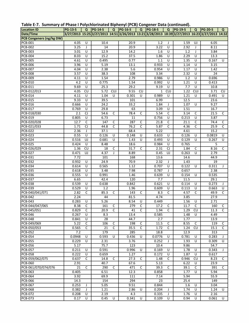
Table E‐7. Summary of Phase I Polychlorinated Biphenyl (PCB) Congener Data (continued).Location ID PG‐13‐S Q PG‐14‐S Q PG‐16‐S Q PG‐18‐S Q PG‐19‐S Q PG‐20‐S QDate/Time 3/27/2013 15:25 3/27/2013 14:51 3/26/2013 13:21 3/28/2013 18:39 3/27/2013 16:23 3/27/2013 14:32PCB Congeners (ng/kg DW)PCB‐001 4.05 U 10.4 20.9 1.2 J 1.59 UJ 6.05PCB‐002 3.25 J 14 20.9 3.22 U 2.92 J 8.11PCB‐003 3.01 U 12.9 14.2 1.6 U 1.2 J 3.84PCB‐004 8.03 U 15.2 37.5 1.86 U 2.29 U 13.3PCB‐005 4.61 U 0.495 0.77 1.1 U 1.35 U 0.167 UPCB‐006 3.96 U 5.19 13.1 0.933 U 1.14 U 3.15PCB‐007 4.04 U 2.38 5.6 0.954 U 1.17 U 1.42PCB‐008 3.57 U 38.3 108 3.34 2.32 U 24PCB‐009 4.11 U 1.54 2.79 0.986 U 1.2 U 0.696PCB‐010 4.2 U 0.775 1.54 0.992 U 1.21 U 0.413PCB‐011 9.69 U 25.3 29.2 9.19 U 7.7 U 10.8PCB‐012/013 4.05 CU 5.72 CUJ 9.55 CU 1 CUJ 1.22 CUJ 3.71 CUPCB‐014 4.11 U 1.04 U 0.301 U 0.989 U 1.21 U 0.491 UPCB‐015 9.33 U 39.5 101 6.99 12.5 23.6PCB‐016 0.666 U 24.2 33.2 1.84 J 1.07 U 9.27PCB‐017 0.769 U 29.8 63 3.09 U 1.51 16.7PCB‐018/030 2.1 CJ 54.6 C 78.4 C 5.54 C 3.14 C 21.5 CPCB‐019 0.805 U 6.73 11 0.756 U 0.213 U 3.87PCB‐020/028 12.7 C 147 C 287 C 21.8 C 21.1 C 74.4 CPCB‐021/033 1.71 CJ 44.8 C 76.2 C 5.87 C 4.36 C 25.9 CPCB‐022 2.36 J 37.1 68.4 5.22 4.61 15.2PCB‐023 0.55 U 0.126 U 0.148 U 0.633 U 0.126 U 0.0819 UPCB‐024 0.516 UJ 0.681 U 1.43 U 0.493 U 0.129 U 0.267 UPCB‐025 0.424 U 8.48 18.6 0.984 U 0.765 5PCB‐026/029 1.36 CU 18 C 31.7 C 2.31 CJ 1.84 C 8.16 CPCB‐027 0.471 UJ 4.37 J 8.89 0.45 UJ 0.263 U 2.79PCB‐031 7.72 101 168 13.6 14.6 44.9PCB‐032 0.932 U 24.9 70.9 2.32 J 1.43 19PCB‐034 0.614 U 0.565 1.12 0.707 U 0.122 U 0.311 JPCB‐035 0.618 U 3.48 7.98 0.787 J 0.657 2.38PCB‐036 0.555 U 0.991 1.46 0.639 U 0.154 U 0.535PCB‐037 6.65 42.4 120 7.7 11.5 29.1PCB‐038 0.539 U 0.638 0.842 0.621 U 0.114 U 0.273 JPCB‐039 0.529 U 1.2 1.96 0.609 U 0.113 U 0.663 UPCB‐040/041/071 2.82 C 85.3 C 143 C 8.3 C 4.57 C 49.9 CPCB‐042 2.24 44 81.5 4.74 3.85 27.9PCB‐043 0.283 U 5.26 8.54 U 0.449 1.56 U 2.71PCB‐044/047/065 8.38 C 161 C 279 C 17.2 C 11.7 C 160 CPCB‐045/051 0.829 C 20.9 C 41 C 1.94 C 1.29 CU 11.3 CPCB‐046 0.267 U 8.3 13.4 0.585 1.48 U 4.49PCB‐048 0.841 U 28 44.7 2.7 1.77 13.9PCB‐049/069 5.22 C 106 C 198 C 11.5 C 8.55 C 119 CPCB‐050/053 0.565 C 21 C 35.5 C 1.72 C 1.24 CU 15.1 CPCB‐052 7.2 179 285 18.8 12.9 313PCB‐054 0.0948 U 0.593 U 0.436 U 0.0776 U 0.781 U 0.283 JPCB‐055 0.229 U 2.31 3.76 0.252 J 1.93 U 0.309 UPCB‐056 5.17 75.7 123 10.4 9.86 54.7PCB‐057 0.211 U 0.591 0.996 U 0.169 U 1.78 U 0.343 JPCB‐058 0.222 U 0.659 1.27 0.172 U 1.87 U 0.617PCB‐059/062/075 0.637 C 14.8 C 27.3 C 1.48 C 0.946 CU 8.23 CPCB‐060 2.91 40.7 67.6 5.13 6.22 U 23.9PCB‐061/070/074/076 21 C 290 C 471 C 39.3 C 39.1 C 391 CPCB‐063 0.405 6.51 12.3 0.858 1.77 U 5.94PCB‐064 3.92 69.9 111 7.14 5.94 55.9PCB‐066 14.3 154 294 23 25.4 149PCB‐067 0.253 J 5.05 9.51 0.844 1.6 U 3.04PCB‐068 0.382 J 1.21 2.86 U 0.204 J 1.74 U 1.24 UPCB‐072 0.208 U 2.19 4.3 0.335 J 1.76 U 2.16PCB‐073 0.17 U 0.45 U 0.341 U 0.109 U 0.94 U 0.061 U

Location ID PG‐13‐S Q PG‐14‐S Q PG‐16‐S Q PG‐18‐S Q PG‐19‐S Q PG‐20‐S QDate/Time 3/27/2013 15:25 3/27/2013 14:51 3/26/2013 13:21 3/28/2013 18:39 3/27/2013 16:23 3/27/2013 14:32PCB‐077 2.28 16.7 54.9 3.24 4.94 U 16.4PCB‐078 0.208 U 0.527 U 0.655 U 0.165 U 1.76 U 0.279 UPCB‐079 0.179 U 2.87 7.18 0.451 1.51 U 5.75PCB‐080 0.205 U 0.518 U 0.622 U 0.157 U 1.72 U 0.263 UPCB‐081 0.173 U 0.868 U 2.04 U 0.175 U 1.82 U 0.884 UPCB‐082 0.946 UJ 21.1 J 58.6 2.19 J 1.84 46.7 JPCB‐083/099 6.9 C 126 C 358 C 16.1 C 11.6 C 282 CPCB‐084 1.51 44.9 117 5.01 2.36 161PCB‐085/116/117 2.15 C 38.3 C 106 C 5.11 C 4.16 CU 88.9 CPCB‐087/097/108/119/125 8.39 C 129 C 316 C 16.2 C 12.6 C 365 CPCB‐088/091 0.979 C 26.5 C 71.1 C 3.17 C 1.81 CU 73.3 CPCB‐089 0.113 U 2.11 7.44 0.253 U 0.229 U 4.38PCB‐090/101/113 9.16 C 203 C 521 C 23.6 C 15.9 C 535 CPCB‐092 1.7 36.1 93.1 4.97 2.78 94.4PCB‐093/095/098/100/102 5.59 C 147 C 365 C 17.7 C 8.93 CU 485 CPCB‐094 0.116 U 1.1 U 3.01 0.096 U 0.235 U 2.1PCB‐096 0.0678 U 1.32 3.21 0.138 J 0.115 U 2.73PCB‐103 0.0946 U 2.51 8.16 0.352 J 0.192 U 4.29PCB‐104 0.068 U 0.058 J 0.134 U 0.0517 U 0.105 U 0.0592 UPCB‐105 6.13 81.6 220 11.2 11 173PCB‐106 0.102 U 0.266 U 0.452 U 0.106 U 0.177 U 0.397 UPCB‐107/124 0.466 C 7.02 C 18.5 C 0.914 C 0.757 CU 15.2 CPCB‐109 0.919 14.8 41.4 2.01 1.54 28PCB‐110/115 12.5 C 225 C 555 C 27.7 C 19.7 C 624 CPCB‐111 0.676 U 0.26 J 0.687 0.0641 U 0.158 U 0.163 UPCB‐112 0.0774 U 0.121 U 0.112 U 0.0651 U 0.157 U 0.123 UPCB‐114 0.294 U 4.49 9.87 0.516 0.537 U 7.23PCB‐118 13.5 188 520 25.7 23.6 415PCB‐120 0.0718 U 1.32 3.52 0.135 J 0.146 U 1.16 UPCB‐121 0.081 U 0.126 U 0.301 U 0.0655 U 0.164 U 0.123 JPCB‐122 0.134 U 2.19 6.42 0.263 U 0.259 U 4.43PCB‐123 0.272 U 3.96 U 9.98 0.604 U 0.508 U 6.49 UPCB‐126 0.113 U 0.984 3.32 U 0.225 J 0.211 U 1.06PCB‐127 0.103 U 0.472 0.42 U 0.101 U 0.178 U 0.422 UPCB‐128/166 1.61 C 29 C 116 C 4.22 C 2.62 C 60.1 CPCB‐129/138/160/163 8.56 C 196 C 727 C 27.6 C 15.9 C 350 CPCB‐130 0.584 12.7 48.9 1.75 0.856 U 23.1PCB‐131 0.1 U 2 6.99 0.2 J 0.332 U 4.86PCB‐132 2.08 55.3 219 7.61 3.75 131PCB‐133 0.177 U 3.4 12.5 0.531 0.314 U 5PCB‐134/143 0.223 CU 8.37 C 34.2 C 1.04 C 0.489 CU 20.1 CPCB‐135/151/154 1.99 C 61.5 C 239 C 7.81 C 3.8 C 95.8 CPCB‐136 0.56 U 17.4 77 2.43 0.768 41.7PCB‐137 0.344 U 7.22 17.2 0.933 0.746 U 15.6PCB‐139/140 0.099 CU 3.36 C 13.3 C 0.431 C 0.3 CU 6.62 CPCB‐141 1.09 27.3 60 3.6 1.87 37PCB‐142 0.098 U 0.245 U 0.88 U 0.173 U 0.324 U 0.368 UPCB‐144 0.171 J 7.77 27.3 0.822 0.418 U 12.4PCB‐145 0.062 U 0.0715 U 0.249 U 0.062 U 0.179 U 0.16 UPCB‐146 1.39 30.3 105 4.94 2.29 46.9PCB‐147/149 3.68 C 137 C 519 C 15 C 8.4 C 253 CPCB‐148 0.0758 U 0.328 J 1.62 0.0766 U 0.218 U 0.385 UPCB‐150 0.0593 U 0.481 U 2.13 0.0601 U 0.171 U 0.765PCB‐152 0.0577 U 0.152 J 0.657 0.058 U 0.166 U 0.384 JPCB‐153/168 7.46 C 173 C 644 C 24.6 C 12.7 C 265 CPCB‐155 0.0517 U 0.123 J 0.227 U 0.048 U 0.129 U 0.095 UPCB‐156/157 1.19 C 18.7 C 61.6 C 2.84 C 2.03 C 31.3 CPCB‐158 0.839 17.6 58.1 2.53 1.49 32PCB‐159 0.0667 U 1.67 6.53 0.207 U 0.22 U 2.22PCB‐161 0.07 U 0.175 U 0.572 U 0.118 U 0.231 U 0.257 UPCB‐162 0.0726 U 0.608 2.44 0.12 U 0.24 U 1.1

Location ID PG‐13‐S Q PG‐14‐S Q PG‐16‐S Q PG‐18‐S Q PG‐19‐S Q PG‐20‐S QDate/Time 3/27/2013 15:25 3/27/2013 14:51 3/26/2013 13:21 3/28/2013 18:39 3/27/2013 16:23 3/27/2013 14:32PCB‐164 0.491 12.2 46.9 1.84 0.873 U 21.7PCB‐165 0.0766 U 0.301 U 1.23 U 0.135 U 0.253 U 0.36 JPCB‐167 0.425 7.08 24.9 1.13 0.663 U 11.5PCB‐169 0.0668 U 0.176 U 0.622 U 0.121 U 0.224 U 0.258 UPCB‐170 1.41 32.2 115 5.86 2.1 43PCB‐171/173 0.533 C 10.4 C 55.8 C 1.86 C 0.525 C 14.6 CPCB‐172 0.285 J 5.94 21.9 1.05 0.536 6.83PCB‐174 1.15 32.8 144 5.22 1.96 U 39PCB‐175 0.0804 U 1.68 8.49 0.205 U 0.19 U 2.18PCB‐176 0.157 J 4.41 23.7 0.606 0.198 U 5.81PCB‐177 0.837 22.2 124 3.78 1.2 30.2PCB‐178 0.378 J 9.94 53.5 1.59 0.534 U 12.3PCB‐179 0.478 14.9 87.5 2.1 0.923 20.3PCB‐180/193 3.03 C 73.9 C 223 C 12.7 C 4.75 C 82.5 CPCB‐181 0.0834 U 0.313 U 1.72 0.0937 U 0.197 U 0.512PCB‐182 0.0809 U 0.335 U 1.42 0.0906 U 0.191 U 0.463PCB‐183/185 0.97 C 26 C 124 C 4.07 C 1.72 C 31.4 CPCB‐184 0.0613 U 0.185 J 0.433 U 0.0698 U 0.145 U 0.113 UPCB‐186 0.0668 U 0.0751 U 0.184 U 0.0755 U 0.158 U 0.116 UPCB‐187 2.3 55.8 300 9.09 3.6 69.4PCB‐188 0.0581 U 0.191 U 0.927 0.071 J 0.138 U 0.275 UPCB‐189 0.128 U 1.31 U 4.51 0.273 U 0.28 U 1.82 UPCB‐190 0.304 J 5.93 25.3 1.07 0.479 U 7.16PCB‐191 0.0643 U 1.29 5.33 0.217 J 0.152 U 1.73PCB‐192 0.0708 U 0.0795 U 0.197 U 0.0802 U 0.167 U 0.126 UPCB‐194 0.669 16.5 54.5 3.2 1.21 22.9PCB‐195 0.247 J 6.15 27.7 1.22 0.391 J 9.07PCB‐196 0.306 J 9.44 43.5 1.76 U 0.577 12.6PCB‐197/199 0.139 CU 2.97 C 16.9 C 0.564 C 0.268 CU 5.13 CPCB‐198/201 0.99 CU 24.5 C 132 C 4.79 C 1.56 CU 34.9 CPCB‐200 0.081 U 3.09 17.1 0.525 0.197 J 3.88PCB‐202 0.282 J 5.81 32.6 1.13 0.438 U 9PCB‐203 0.591 U 13.4 61.2 2.58 1.01 U 17.5PCB‐204 0.0551 U 0.0664 U 0.145 U 0.0719 U 0.154 U 0.105 UPCB‐205 0.0944 U 0.823 4.3 0.186 U 0.258 U 1.16PCB‐206 0.547 15.9 63.7 2.62 0.925 U 20.2PCB‐207 0.208 U 2.17 9.46 0.415 U 0.619 U 2.56PCB‐208 0.23 U 6.49 29.1 0.871 U 0.647 U 8.08PCB‐209 0.533 25.1 67.5 2.11 1.19 U 18.5Total PCBs* 231 4620 12100 582 382 7220PCB TEQ (0 DL) 0.000865 0.109 0.031 0.0241 0.0011 0.127PCB TEQ (1/2 DL) 0.00755 0.112 0.207 0.0259 0.0156 0.131PCB TEQ (1 DL) 0.0142 0.115 0.382 0.0278 0.03 0.135PCB TEQ (KM) 0.012 L6 0.11 0.37 L 0.024 0.023 L8 0.13*total PCBs represents the sum of all detected congenersU‐the analytie was analyzed for, but was not detected above the reported sample quantitation limiJ‐the analyte was positively identified; the associated numerical value is the approximate concentration of the analyte in the samplUJ‐the analyte was not detected above the reported sample quantitation limit. However, the reported quantitation limit is approximateL‐the detection frequency of compounds within a sample was <50%, the numeric value indicates the number of non‐detectKM‐Kaplan‐Meier DW‐dry weight Q‐qualifier TEQ‐toxicity equivalent DL‐detection limit Avg‐average of field duplicatesC‐see list for co‐eluting congeners

Table E‐7. Summary of Phase I Polychlorinated Biphenyl (PCB) Congener Data (continued).Location ID PG‐22‐S Q PG‐24‐S Q PG‐25‐S Q PG‐26‐S Q PG‐29‐S Q PG‐30‐S QDate/Time 3/27/2013 11:29 3/26/2013 15:21 3/28/2013 18:55 3/26/2013 16:53 3/26/2013 15:43 3/27/2013 16:04PCB Congeners (ng/kg DW)PCB‐001 0.876 11.2 1.19 U 6.24 5.21 2.24 UPCB‐002 1.95 18 3.43 17.6 11.8 2.56 UPCB‐003 0.985 U 10.5 1.87 U 7.27 6.45 1.73 UPCB‐004 2.57 17.6 1.31 7.43 7.81 3.64 UPCB‐005 0.213 U 0.585 0.183 U 0.394 J 0.397 J 2.18 UPCB‐006 0.549 U 6.21 0.754 4.04 3.8 1.89 UPCB‐007 0.294 U 3.06 0.25 U 1.36 1.35 1.96 UPCB‐008 3.58 49.1 4.86 22 24.8 4.47PCB‐009 0.19 U 1.66 0.223 U 1.05 0.962 1.88 UPCB‐010 0.199 U 0.724 0.173 U 0.338 U 0.327 J 1.89 UPCB‐011 2.45 U 27.3 11.4 33.3 22.7 6.28PCB‐012/013 5.22 CU 9.48 CUJ 5.2 CUJ 6.65 CU 6.34 CU 13.1 CUPCB‐014 0.191 U 0.586 U 0.239 U 0.508 U 0.418 U 1.96 UPCB‐015 3.27 58.9 14.5 32.9 35 15.1PCB‐016 1.71 18.9 2.1 U 10.2 9.18 2.22 UPCB‐017 2.94 30.9 2.22 14.3 15 2.3 UPCB‐018/030 4.25 C 42.2 C 4.95 C 23.2 C 24.3 C 3.14 CPCB‐019 0.811 5.08 0.519 2.72 2.61 2.02 UPCB‐020/028 9.98 C 165 C 28.8 C 89.4 C 91.8 C 25.1 CPCB‐021/033 2.65 C 46.4 C 8.77 C 29.2 C 29 C 7.21 CPCB‐022 2.23 37.1 8.44 23.6 23.4 7.48PCB‐023 0.0845 U 0.1 U 0.0687 U 0.338 U 0.196 U 1.61 UPCB‐024 0.0661 U 0.511 0.759 U 0.312 J 0.296 J 1.28 UPCB‐025 0.672 9.62 1.57 5.67 5.51 1.36 UPCB‐026/029 1.16 C 17.8 C 3.11 C 11 C 11 C 2.23 CPCB‐027 0.518 J 4.48 J 0.757 UJ 2.45 2.72 1.26 UPCB‐031 5.88 99.1 18.8 58.8 59 13.9PCB‐032 3.82 30.5 2.49 10.4 12.6 1.45 UPCB‐034 0.0803 U 0.748 0.076 U 0.361 J 0.497 1.52 UPCB‐035 0.272 J 5.04 1.2 2.98 3 1.61 UPCB‐036 0.111 U 1.13 0.31 J 0.818 0.839 1.44 UPCB‐037 3.75 65.1 13.5 32.2 35.9 13.2PCB‐038 0.0732 U 0.476 0.132 U 0.317 U 0.351 J 1.51 UPCB‐039 0.092 J 1.15 0.114 U 0.751 U 0.634 1.5 UPCB‐040/041/071 5.97 C 75.5 C 10 C 33.7 C 40.8 C 4.83 CPCB‐042 3.17 41.8 6.15 19.9 22.8 2.7PCB‐043 0.297 U 4.54 0.385 U 1.73 2.58 0.251 UPCB‐044/047/065 11.2 C 149 C 20.6 C 69.3 C 83.4 C 8.82 CPCB‐045/051 1.97 C 19.7 C 2.29 C 8.25 C 9.91 C 0.998 CPCB‐046 0.749 6.4 0.774 2.76 3.28 0.341 JPCB‐048 1.77 23.8 2.54 10.5 13 1.18PCB‐049/069 7.71 C 106 C 13.3 C 51.7 C 60.2 C 5.58 CPCB‐050/053 1.93 C 16.6 C 1.96 C 7.26 C 9.09 C 0.87 CPCB‐052 12.6 164 22.2 80.2 94.6 7.67PCB‐054 0.0635 U 0.307 U 0.263 U 0.334 J 0.163 J 0.132 UPCB‐055 0.114 U 2.67 0.579 U 1.43 1.47 0.207 UPCB‐056 4.84 78.7 14.5 42.7 45.3 8.49PCB‐057 0.105 U 0.731 U 0.565 U 0.481 U 0.431 0.196 UPCB‐058 0.108 U 0.742 U 0.575 U 0.573 0.505 0.203 UPCB‐059/062/075 1.11 C 13.9 C 2.08 C 5.97 C 7.22 C 0.98 CPCB‐060 2.45 40.3 7.67 21.4 22.7 4.51PCB‐061/070/074/076 18.5 C 305 C 55 C 170 C 181 C 26.1 CPCB‐063 0.466 7.62 1.08 3.76 4.27 0.403 JPCB‐064 4.43 61.1 8.34 29.9 34.5 4.32PCB‐066 10.7 185 33.8 102 110 18.6PCB‐067 0.376 5.62 0.982 3.16 3.52 0.457PCB‐068 0.126 J 1.59 0.546 U 1.12 1.12 0.19 UPCB‐072 0.133 U 2.7 0.567 U 1.52 1.63 0.188 JPCB‐073 0.0644 U 0.0731 U 0.269 U 0.365 U 0.362 J 0.137 U

Location ID PG‐22‐S Q PG‐24‐S Q PG‐25‐S Q PG‐26‐S Q PG‐29‐S Q PG‐30‐S QDate/Time 3/27/2013 11:29 3/26/2013 15:21 3/28/2013 18:55 3/26/2013 16:53 3/26/2013 15:43 3/27/2013 16:04PCB‐077 2.09 29.3 5.46 13 15.3 2.39PCB‐078 0.103 U 0.304 U 0.551 U 0.507 U 0.24 U 0.196 UPCB‐079 0.197 J 4.06 0.63 1.94 2.3 0.359 UPCB‐080 0.0971 U 0.287 U 0.523 U 0.472 U 0.222 U 0.181 UPCB‐081 0.112 U 1.07 U 0.59 U 0.566 U 0.555 U 0.189 UPCB‐082 2.24 34 4.5 14.8 20.8 1.22 JPCB‐083/099 15.5 C 198 C 21.5 C 90.6 C 111 C 6.52 CPCB‐084 4.65 65.9 6.26 26.3 35.9 2.05PCB‐085/116/117 4.39 C 60.5 C 7.06 C 27.4 C 35 C 2.4 CPCB‐087/097/108/119/125 13.8 C 190 C 22.9 C 84.7 C 106 C 7.1 CPCB‐088/091 3.03 C 41.2 C 3.76 C 17.7 C 23.6 C 1.26 CPCB‐089 0.293 U 3.92 0.278 J 1.15 1.73 0.222 UPCB‐090/101/113 21.1 C 293 C 32.2 C 133 C 164 C 8.36 CPCB‐092 3.75 54.4 6.07 26.4 32 1.57PCB‐093/095/098/100/102 17 C 218 C 24.2 C 93.4 C 123 C 5.71 CPCB‐094 0.15 U 1.63 0.146 U 0.752 0.795 0.232 UPCB‐096 0.171 U 1.61 0.126 U 0.599 0.95 0.129 UPCB‐103 0.363 4.41 0.411 2.07 2.54 0.186 UPCB‐104 0.0616 U 0.065 U 0.0493 U 0.233 U 0.106 U 0.119 UPCB‐105 8.42 128 18.5 61.2 73.9 6.32PCB‐106 0.112 U 0.22 U 0.118 U 0.626 U 0.308 U 0.261 UPCB‐107/124 0.758 CU 10.5 C 1.6 C 5.25 C 6.21 C 0.505 CPCB‐109 1.64 24.5 2.99 11.7 14 0.911PCB‐110/115 22.2 C 331 C 38.8 C 145 C 192 C 12 CPCB‐111 0.104 U 0.438 0.0569 U 0.312 U 0.217 U 0.159 UPCB‐112 0.104 U 0.116 U 0.0578 U 0.315 U 0.199 U 0.157 UPCB‐114 0.314 6.23 0.873 3.07 3.5 0.388 JPCB‐118 20.1 301 42.1 144 176 13.5PCB‐120 0.133 J 1.98 0.25 J 1.14 1.24 0.147 UPCB‐121 0.104 U 0.204 U 0.0581 U 0.309 U 0.201 U 0.159 UPCB‐122 0.239 U 3.77 0.514 1.72 1.98 0.271 UPCB‐123 0.381 5.91 0.952 U 2.69 3.47 0.305 UPCB‐126 0.136 U 1.82 0.253 J 0.939 U 1.09 0.298 UPCB‐127 0.119 U 0.234 U 0.113 U 0.634 U 0.299 U 0.253 UPCB‐128/166 3.98 C 66.3 C 6.09 C 30.4 C 39.3 C 1.59 CPCB‐129/138/160/163 26.3 C 412 C 37.3 C 194 C 237 C 9 CPCB‐130 1.8 27.7 2.36 12.3 15.2 0.54PCB‐131 0.242 U 4.27 0.298 J 2.14 2.42 0.262 UPCB‐132 7.07 123 9.52 52.5 69.4 2.12PCB‐133 0.478 7.05 0.759 3.85 4.17 0.246 UPCB‐134/143 1.08 CU 18.8 C 1.35 C 6.98 C 10.3 C 0.256 CUPCB‐135/151/154 7.7 C 123 C 10.3 C 56.5 C 69.4 C 1.89 CPCB‐136 2.53 39.7 2.73 16.2 22.1 0.481PCB‐137 0.904 10.8 1.38 7.76 7.23 0.444 UPCB‐139/140 0.461 CU 7.3 C 0.632 C 3.3 C 4.35 C 0.234 CUPCB‐141 2.72 34.4 4.93 22.9 22.4 1.06PCB‐142 0.155 U 0.245 U 0.113 U 0.702 U 0.305 U 0.259 UPCB‐144 0.788 U 14.2 1.05 U 6.11 7.57 0.328 JPCB‐145 0.0868 U 0.103 J 0.0632 U 0.318 U 0.201 U 0.15 UPCB‐146 4.38 68.7 J 6.17 34.1 37.9 1.36PCB‐147/149 18.9 C 296 C 17.3 C 131 C 163 C 4.29 CPCB‐148 0.107 U 1.05 0.086 J 0.879 U 1.11 U 0.188 UPCB‐150 0.086 U 1.02 0.067 U 0.554 U 0.608 0.149 UPCB‐152 0.081 U 0.325 U 0.0591 U 0.288 U 0.234 J 0.136 UPCB‐153/168 24.3 C 361 C 32.5 C 170 C 204 C 6.61 CPCB‐155 0.07 U 0.133 U 0.0475 U 0.225 U 0.147 U 0.113 UPCB‐156/157 2.17 C 35.6 C 3.87 C 17.6 C 21.2 C 1.19 CUPCB‐158 1.91 33.8 3.45 15.2 19 0.976PCB‐159 0.239 U 4.03 0.344 J 1.71 1.89 0.18 UPCB‐161 0.109 U 0.171 U 0.0767 U 0.507 U 0.207 U 0.176 UPCB‐162 0.109 U 1.77 0.143 J 1 U 0.217 U 0.184 U

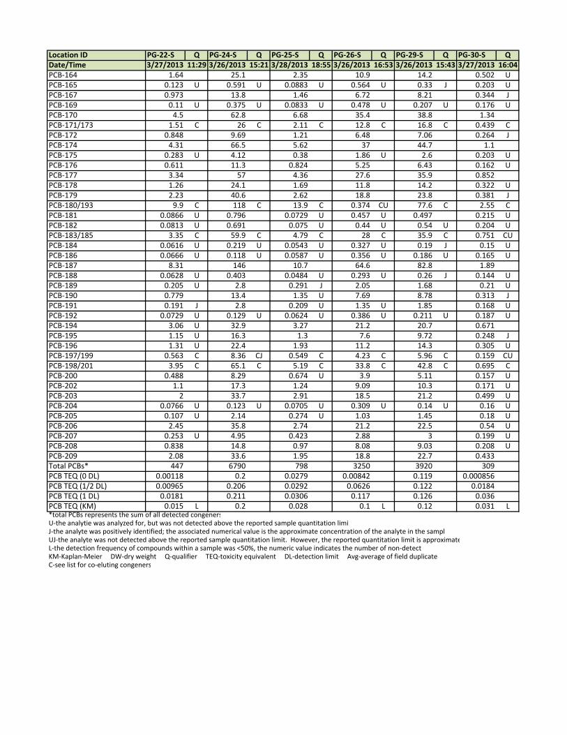
Location ID PG‐22‐S Q PG‐24‐S Q PG‐25‐S Q PG‐26‐S Q PG‐29‐S Q PG‐30‐S QDate/Time 3/27/2013 11:29 3/26/2013 15:21 3/28/2013 18:55 3/26/2013 16:53 3/26/2013 15:43 3/27/2013 16:04PCB‐164 1.64 25.1 2.35 10.9 14.2 0.502 UPCB‐165 0.123 U 0.591 U 0.0883 U 0.564 U 0.33 J 0.203 UPCB‐167 0.973 13.8 1.46 6.72 8.21 0.344 JPCB‐169 0.11 U 0.375 U 0.0833 U 0.478 U 0.207 U 0.176 UPCB‐170 4.5 62.8 6.68 35.4 38.8 1.34PCB‐171/173 1.51 C 26 C 2.11 C 12.8 C 16.8 C 0.439 CPCB‐172 0.848 9.69 1.21 6.48 7.06 0.264 JPCB‐174 4.31 66.5 5.62 37 44.7 1.1PCB‐175 0.283 U 4.12 0.38 1.86 U 2.6 0.203 UPCB‐176 0.611 11.3 0.824 5.25 6.43 0.162 UPCB‐177 3.34 57 4.36 27.6 35.9 0.852PCB‐178 1.26 24.1 1.69 11.8 14.2 0.322 UPCB‐179 2.23 40.6 2.62 18.8 23.8 0.381 JPCB‐180/193 9.9 C 118 C 13.9 C 0.374 CU 77.6 C 2.55 CPCB‐181 0.0866 U 0.796 0.0729 U 0.457 U 0.497 0.215 UPCB‐182 0.0813 U 0.691 0.075 U 0.44 U 0.54 U 0.204 UPCB‐183/185 3.35 C 59.9 C 4.79 C 28 C 35.9 C 0.751 CUPCB‐184 0.0616 U 0.219 U 0.0543 U 0.327 U 0.19 J 0.15 UPCB‐186 0.0666 U 0.118 U 0.0587 U 0.356 U 0.186 U 0.165 UPCB‐187 8.31 146 10.7 64.6 82.8 1.89PCB‐188 0.0628 U 0.403 0.0484 U 0.293 U 0.26 J 0.144 UPCB‐189 0.205 U 2.8 0.291 J 2.05 1.68 0.21 UPCB‐190 0.779 13.4 1.35 U 7.69 8.78 0.313 JPCB‐191 0.191 J 2.8 0.209 U 1.35 U 1.85 0.168 UPCB‐192 0.0729 U 0.129 U 0.0624 U 0.386 U 0.211 U 0.187 UPCB‐194 3.06 U 32.9 3.27 21.2 20.7 0.671PCB‐195 1.15 U 16.3 1.3 7.6 9.72 0.248 JPCB‐196 1.31 U 22.4 1.93 11.2 14.3 0.305 UPCB‐197/199 0.563 C 8.36 CJ 0.549 C 4.23 C 5.96 C 0.159 CUPCB‐198/201 3.95 C 65.1 C 5.19 C 33.8 C 42.8 C 0.695 CPCB‐200 0.488 8.29 0.674 U 3.9 5.11 0.157 UPCB‐202 1.1 17.3 1.24 9.09 10.3 0.171 UPCB‐203 2 33.7 2.91 18.5 21.2 0.499 UPCB‐204 0.0766 U 0.123 U 0.0705 U 0.309 U 0.14 U 0.16 UPCB‐205 0.107 U 2.14 0.274 U 1.03 1.45 0.18 UPCB‐206 2.45 35.8 2.74 21.2 22.5 0.54 UPCB‐207 0.253 U 4.95 0.423 2.88 3 0.199 UPCB‐208 0.838 14.8 0.97 8.08 9.03 0.208 UPCB‐209 2.08 33.6 1.95 18.8 22.7 0.433Total PCBs* 447 6790 798 3250 3920 309PCB TEQ (0 DL) 0.00118 0.2 0.0279 0.00842 0.119 0.000856PCB TEQ (1/2 DL) 0.00965 0.206 0.0292 0.0626 0.122 0.0184PCB TEQ (1 DL) 0.0181 0.211 0.0306 0.117 0.126 0.036PCB TEQ (KM) 0.015 L 0.2 0.028 0.1 L 0.12 0.031 L*total PCBs represents the sum of all detected congenersU‐the analytie was analyzed for, but was not detected above the reported sample quantitation limiJ‐the analyte was positively identified; the associated numerical value is the approximate concentration of the analyte in the samplUJ‐the analyte was not detected above the reported sample quantitation limit. However, the reported quantitation limit is approximateL‐the detection frequency of compounds within a sample was <50%, the numeric value indicates the number of non‐detectKM‐Kaplan‐Meier DW‐dry weight Q‐qualifier TEQ‐toxicity equivalent DL‐detection limit Avg‐average of field duplicatesC‐see list for co‐eluting congeners

Table E‐7. Summary of Phase I Polychlorinated Biphenyl (PCB) Congener Data (continued).Location ID PG‐32‐S Q PG‐33‐S Q PG‐35‐S Q PG‐58‐S QDate/Time 3/26/2013 13:46 3/28/2013 17:22 3/27/2013 10:53 4/22/2014 10:46PCB Congeners (ng/kg DW)PCB‐001 11.9 1.23 U 1.94 U 9.48PCB‐002 15.9 3.26 2.79 J 11.7PCB‐003 11.2 1.45 J 1.27 U 11.4PCB‐004 20.8 13 U 14.4 U 10PCB‐005 0.507 7.31 U 9.95 U 0.834PCB‐006 6.24 6.35 U 8.64 U 8.03PCB‐007 2.97 6.51 U 8.86 U 2PCB‐008 49.1 6 U 8.16 U 43.9PCB‐009 1.5 6.21 U 8.46 U 2.09PCB‐010 0.815 6.08 U 8.27 U 0.495PCB‐011 24.8 7.99 U 9.29 U 20.4PCB‐012/013 8.39 CU 7.26 CU 9.88 CU 7.07 CPCB‐014 0.744 6.64 U 9.03 U 0.399PCB‐015 57 8.33 U 10.8 U 40.4PCB‐016 16.9 4.57 UJ 2.15 U 25.2PCB‐017 31.6 1.59 UJ 1.93 U 31.3PCB‐018/030 44.2 C 2.57 CJ 3.19 C 51 CJPCB‐019 6.11 1.39 U 1.78 U 4.52PCB‐020/028 164 C 13.2 CJ 7.17 C 180 CPCB‐021/033 44 C 2.53 CJ 2.26 CJ 78.1 CPCB‐022 36.9 3.09 J 1.61 U 55.1PCB‐023 0.177 U 1.31 UJ 1.56 U 0.14 JPCB‐024 0.548 U 1.2 UJ 1.46 U 0.716PCB‐025 10.1 1.1 UJ 1.31 U 16PCB‐026/029 18.4 C 1.38 CJ 1.52 CU 34.4 CPCB‐027 6.32 1.07 UJ 1.31 U 5.04PCB‐031 98.8 24.4 J 4.18 135PCB‐032 31.3 3.07 UJ 1.95 U 24.9PCB‐034 0.722 1.25 UJ 1.49 U 0.91PCB‐035 4.85 1.32 UJ 1.57 U 3.51PCB‐036 1.08 1.22 UJ 1.46 U 0.52PCB‐037 65.1 6.48 J 3.14 54.4PCB‐038 0.526 U 1.26 UJ 1.51 U 0.418PCB‐039 1.13 1.25 UJ 1.49 U 1.18PCB‐040/041/071 76 C 3.1 C 4.34 C 69 CPCB‐042 41.6 2.67 2.22 39PCB‐043 4.94 0.298 U 0.782 U 5.08PCB‐044/047/065 151 C 8.06 C 7.46 C 164 CPCB‐045/051 19.4 C 0.842 C 1.6 C 17.2 CPCB‐046 6.21 0.263 U 0.813 U 5.89PCB‐048 23 0.974 1.11 25.2PCB‐049/069 107 C 5.92 C 5.69 C 117 CPCB‐050/053 17.6 C 0.756 C 1.27 C 14.8 CPCB‐052 160 9.65 8.57 194PCB‐054 0.328 J 0.135 U 0.367 U 0.251 JPCB‐055 2.13 0.199 U 0.647 U 3.65PCB‐056 77.7 5.89 3.07 81.6PCB‐057 0.966 0.189 U 0.569 U 1.87PCB‐058 0.917 U 0.196 U 0.621 U 0.859PCB‐059/062/075 14 C 0.581 C 0.797 CU 14.7 CPCB‐060 42.3 3.16 1.54 U 38.5PCB‐061/070/074/076 304 C 24.7 C 11.9 C 357 CPCB‐063 7.69 0.487 0.579 U 7.68PCB‐064 64.4 4.23 3.07 65.2PCB‐066 192 16.7 7.56 186PCB‐067 6.06 0.304 J 0.53 U 9.67PCB‐068 1.99 0.183 U 0.554 U 2.43PCB‐072 2.75 0.189 U 0.552 U 4.04PCB‐073 0.42 0.163 U 0.559 U 0.0497 U

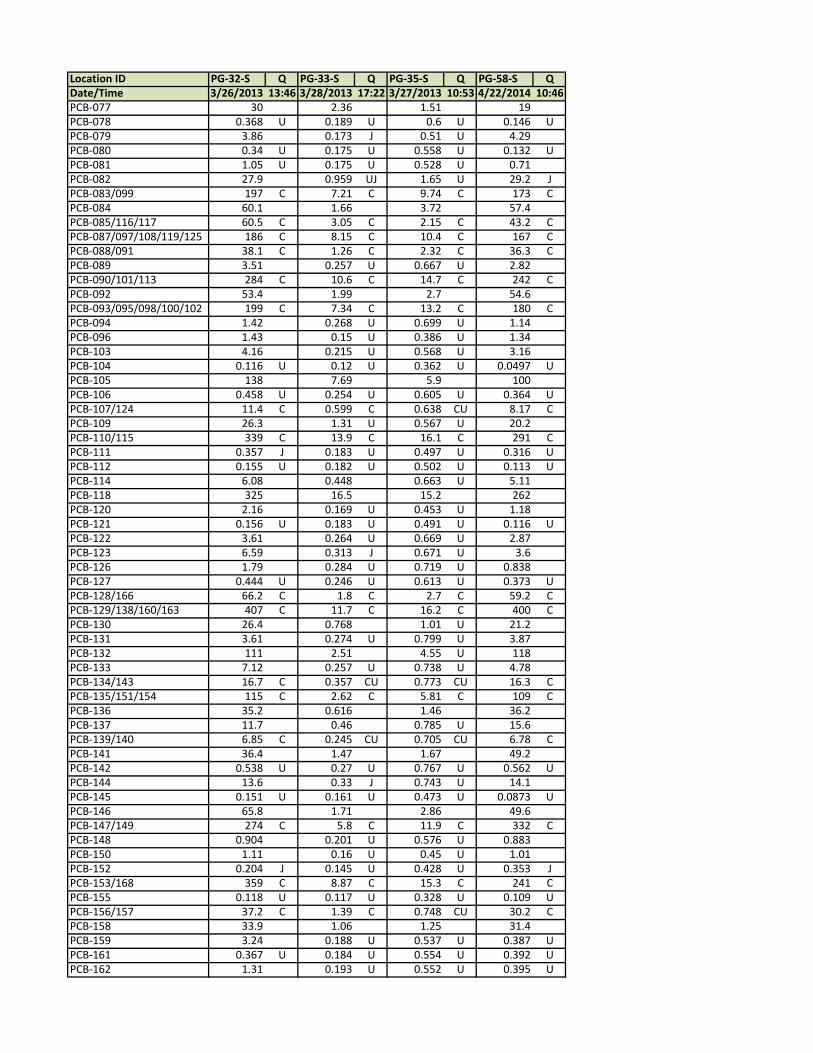
Location ID PG‐32‐S Q PG‐33‐S Q PG‐35‐S Q PG‐58‐S QDate/Time 3/26/2013 13:46 3/28/2013 17:22 3/27/2013 10:53 4/22/2014 10:46PCB‐077 30 2.36 1.51 19PCB‐078 0.368 U 0.189 U 0.6 U 0.146 UPCB‐079 3.86 0.173 J 0.51 U 4.29PCB‐080 0.34 U 0.175 U 0.558 U 0.132 UPCB‐081 1.05 U 0.175 U 0.528 U 0.71PCB‐082 27.9 0.959 UJ 1.65 U 29.2 JPCB‐083/099 197 C 7.21 C 9.74 C 173 CPCB‐084 60.1 1.66 3.72 57.4PCB‐085/116/117 60.5 C 3.05 C 2.15 C 43.2 CPCB‐087/097/108/119/125 186 C 8.15 C 10.4 C 167 CPCB‐088/091 38.1 C 1.26 C 2.32 C 36.3 CPCB‐089 3.51 0.257 U 0.667 U 2.82PCB‐090/101/113 284 C 10.6 C 14.7 C 242 CPCB‐092 53.4 1.99 2.7 54.6PCB‐093/095/098/100/102 199 C 7.34 C 13.2 C 180 CPCB‐094 1.42 0.268 U 0.699 U 1.14PCB‐096 1.43 0.15 U 0.386 U 1.34PCB‐103 4.16 0.215 U 0.568 U 3.16PCB‐104 0.116 U 0.12 U 0.362 U 0.0497 UPCB‐105 138 7.69 5.9 100PCB‐106 0.458 U 0.254 U 0.605 U 0.364 UPCB‐107/124 11.4 C 0.599 C 0.638 CU 8.17 CPCB‐109 26.3 1.31 U 0.567 U 20.2PCB‐110/115 339 C 13.9 C 16.1 C 291 CPCB‐111 0.357 J 0.183 U 0.497 U 0.316 UPCB‐112 0.155 U 0.182 U 0.502 U 0.113 UPCB‐114 6.08 0.448 0.663 U 5.11PCB‐118 325 16.5 15.2 262PCB‐120 2.16 0.169 U 0.453 U 1.18PCB‐121 0.156 U 0.183 U 0.491 U 0.116 UPCB‐122 3.61 0.264 U 0.669 U 2.87PCB‐123 6.59 0.313 J 0.671 U 3.6PCB‐126 1.79 0.284 U 0.719 U 0.838PCB‐127 0.444 U 0.246 U 0.613 U 0.373 UPCB‐128/166 66.2 C 1.8 C 2.7 C 59.2 CPCB‐129/138/160/163 407 C 11.7 C 16.2 C 400 CPCB‐130 26.4 0.768 1.01 U 21.2PCB‐131 3.61 0.274 U 0.799 U 3.87PCB‐132 111 2.51 4.55 U 118PCB‐133 7.12 0.257 U 0.738 U 4.78PCB‐134/143 16.7 C 0.357 CU 0.773 CU 16.3 CPCB‐135/151/154 115 C 2.62 C 5.81 C 109 CPCB‐136 35.2 0.616 1.46 36.2PCB‐137 11.7 0.46 0.785 U 15.6PCB‐139/140 6.85 C 0.245 CU 0.705 CU 6.78 CPCB‐141 36.4 1.47 1.67 49.2PCB‐142 0.538 U 0.27 U 0.767 U 0.562 UPCB‐144 13.6 0.33 J 0.743 U 14.1PCB‐145 0.151 U 0.161 U 0.473 U 0.0873 UPCB‐146 65.8 1.71 2.86 49.6PCB‐147/149 274 C 5.8 C 11.9 C 332 CPCB‐148 0.904 0.201 U 0.576 U 0.883PCB‐150 1.11 0.16 U 0.45 U 1.01PCB‐152 0.204 J 0.145 U 0.428 U 0.353 JPCB‐153/168 359 C 8.87 C 15.3 C 241 CPCB‐155 0.118 U 0.117 U 0.328 U 0.109 UPCB‐156/157 37.2 C 1.39 C 0.748 CU 30.2 CPCB‐158 33.9 1.06 1.25 31.4PCB‐159 3.24 0.188 U 0.537 U 0.387 UPCB‐161 0.367 U 0.184 U 0.554 U 0.392 UPCB‐162 1.31 0.193 U 0.552 U 0.395 U

Location ID PG‐32‐S Q PG‐33‐S Q PG‐35‐S Q PG‐58‐S QDate/Time 3/26/2013 13:46 3/28/2013 17:22 3/27/2013 10:53 4/22/2014 10:46PCB‐164 24 0.69 1.25 U 21.7PCB‐165 0.69 U 0.212 U 0.616 U 0.449 UPCB‐167 14.7 0.445 0.733 10.4PCB‐169 0.359 U 0.181 U 0.526 U 0.325 UPCB‐170 67.9 2.01 2.16 61.9PCB‐171/173 29.4 C 0.737 C 0.857 CU 25.4 CPCB‐172 12.2 0.415 0.658 U 11.1PCB‐174 75.4 1.62 2.11 86.3PCB‐175 4.6 0.233 U 0.608 U 2.68PCB‐176 10.9 0.199 J 0.476 U 11.3PCB‐177 65 1.07 1.94 59.4PCB‐178 26.4 0.525 1.04 U 16.3PCB‐179 42.4 0.73 1.37 U 40.1PCB‐180/193 135 C 4.21 C 4.12 C 139 CPCB‐181 0.981 0.246 U 0.64 U 0.659PCB‐182 0.693 0.233 U 0.616 U 0.611PCB‐183/185 64.6 C 1.09 C 1.93 C 0.157 CUPCB‐184 0.209 J 0.173 U 0.458 U 0.154 JPCB‐186 0.181 U 0.189 U 0.498 U 0.128 UPCB‐187 153 2.84 4.63 134PCB‐188 0.543 0.17 U 0.423 U 0.352 JPCB‐189 2.94 0.257 U 0.686 U 2.47PCB‐190 15.3 0.543 U 0.499 U 13.9PCB‐191 3.34 0.192 U 0.488 U 2.8PCB‐192 0.206 U 0.215 U 0.54 U 0.137 UPCB‐194 37.9 0.957 1.03 U 35.1PCB‐195 17 0.403 J 0.693 U 14PCB‐196 26.6 0.601 U 0.557 16.6PCB‐197/199 10.8 C 0.19 CU 0.41 CU 5.53 CJPCB‐198/201 75.8 C 1.52 C 1.38 C 41 CPCB‐200 8.82 0.189 J 0.396 U 4.87PCB‐202 18 0.381 J 0.524 U 10.2PCB‐203 38.1 0.95 U 0.59 U 25.7PCB‐204 0.162 U 0.19 U 0.411 U 0.0806 UPCB‐205 2.38 0.201 U 0.563 U 1.59PCB‐206 39.6 0.898 U 0.847 U 22.4PCB‐207 5.49 0.262 U 0.671 U 2.62PCB‐208 16.2 0.414 0.71 U 8.02PCB‐209 37.6 0.961 0.749 17Total PCBs* 6840 292 258 6390PCB TEQ (0 DL) 0.198 0.00104 0.000806 0.0983PCB TEQ (1/2 DL) 0.203 0.018 0.0448 0.103PCB TEQ (1 DL) 0.209 0.0349 0.0887 0.108PCB TEQ (KM) 0.2 0.03 L 0.073 L6 0.1*total PCBs represents the sum of all detected congenersU‐the analytie was analyzed for, but was not detected above the reported sample quantitation limiJ‐the analyte was positively identified; the associated numerical value is the approximate concentration of the analyte in the samplUJ‐the analyte was not detected above the reported sample quantitation limit. However, the reported quantitation limit is approximateL‐the detection frequency of compounds within a sample was <50%, the numeric value indicates the number of non‐detectKM‐Kaplan‐Meier DW‐dry weight Q‐qualifier TEQ‐toxicity equivalent DL‐detection limit Avg‐average of field duplicatesC‐see list for co‐eluting congeners

Appendix H. Univariate and Multivariate Investigations of the Port Gardner Bay Data Set

Appendix H: Univariate and Multivariate Investigations of the Port Gardner Bay Data Set

Various statistical methods were used to evaluate the data from Port Gardner Bay. This appendix represents a record of the analyses performed. The analyses in Section H1.0 were conducted to determine the most appropriate distribution for each analyte. All data were evaluated in Section H2.0 to identify if any statistical outliers existed for any of the individual analytes. The bivariate and multivariate exploratory analyses of Sections H3.0 and H4.0 were conducted to further explore patterns in the data and identify any unusual results not obvious from the univariate analysis. Any samples flagged by the analyses of Sections H3.0 and H4.0 were not considered outliers for the purpose of calculating the 90/90 upper tolerance limits (90/90 UTLs).

H.1 Distributional Analysis

The distributions for each analyte were evaluated individually in R (R Core Team 2014) to generate normal-probability plots and in ProUCL 5.0 (USEPA 2013) for formal goodness of fit (GOF) tests against the standard distributions (i.e., normal and gamma). The normal probability plots are shown in Figures H-1 and H-2 for each of the analytes. These plots were used in part to evaluate the shape of the data distribution. The results of the goodness of fit tests (α = 0.05) based on the detected data only, are shown in Table H-1.

Most of the chemical distributions did not deviate significantly from a normal distribution. For cadmium, the distribution could be considered normal with elevated concentrations present, or a skewed gamma distribution provided a good fit to all of the observations. All of the data sets were best described by a normal distribution, except the following:

Dioxin/Furan TEQ – the normal distribution was rejected (Shapiro-Wilks’s test p < 0.03 for detected data), mainly because both tails were shorter than expected for normality (fewer values far out in the tails than expected). The distribution had symmetry like a normal distribution, and no extreme values. Because of the lack of any skewness in these data, the normal distribution was still the best-fitting distribution.

Cadmium – for the detected data, a gamma distribution was the best fit to all of the observations, while a normal distribution was a good fit if location PG-60 was excluded.

H.2 Univariate Investigation of Extreme Values for each Analyte

The term extreme value is used to define a result that deviates from the population mean but may still be representative of background (SCUM II; Ecology 2013). Extreme values are common in data sets that lack sufficient sample sizes to capture the full range of values. Essentially, it is unknown whether an extreme value is an outlier unless more samples are available. The individual analytes were screened for extreme values using a variety of approaches:

Single extreme values were identified using Rosner’s formal outlier test (for n ≥ 25, conducted in ProUCL; α = 0.05) for data that fit a normal distribution (see Table H-1).

Extreme values were also identified when the single highest concentration sample was the difference between a normal and a non-normal distribution (i.e., if the high concentration sample were excluded, the distribution would be normal).

High values were flagged as extreme based on the boxplots for metals in Figure H-3 and the organic analytes in Figure H-4, using Tukey’s rule of thumb1.

Screening for extreme values was done to determine whether specific samples may be skewing the distribution for an individual analyte. A summary of the extreme values for each CoC in the Port Gardner Bay data set follows:

Arsenic and mercury presented no extreme values (Figures H-1 and H-3).

Cadmium presented one extreme value (PG-60) for the formal outlier test (Rosner’s p < 0.05). Tukey’s rule of thumb also identified this sample as extreme (Figure H-3), with a concentration of 0.61 ppm, outside the “whiskers” of the box-and-whisker plot.

cPAH, dioxin/furan, and PCB TEQs presented no extreme values (Figures H-2 and H-4).

Several of the analyte distributions, including the values identified as extreme, were entirely within the range of natural background. If a sample result was identified as extreme, but not outside the range of natural background, there was no need to exclude it from the data set.

H.3 Correlation Between Analyte Concentrations and Conventional Parameters

The following bivariate investigations evaluated the distribution of each analyte in relation to percent fines and percent TOC. Anthropogenic contamination tends to be associated with these conventional parameters, so in urban embayments there is typically a positive correlation with

1 Tukey’s rule of thumb flags values as extreme when they exceed the median ± 1.5 × IQR (IQR = interquartile range = 3rd quartile minus the 1st quartile). These points fall outside the whiskers on the boxplots.

these parameters. Deviations from the general trend can be indicative of a different source, or a different geochemical/depositional environment. This exploratory investigation provided information for understanding some of the possible sediment dynamics in Port Gardner Bay, but was not a deciding factor in excluding samples as outliers.

The correlation between percent fines and percent TOC was strong (Pearson’s r = 0.75, df = 28, p < 0.001). The scatterplot for this correlation is shown in Figure H-5. The 5 labeled samples are discussed in Sections 3.1 and 3.2.

H.3.1 Correlations with Grain Size

The relationships between grain size (as percent fines) and analyte concentrations are presented graphically as scatterplots in Figure H-6. The grain size for the samples in this data set were evenly distributed throughout the observed range of 4 to 97 percent fines, which provided a good description of the relationship between Port Gardner Bay sediment chemistry and percent fines for sediment types ranging from coarse to fine grained. The scatterplots showed strong correlations between each of the analytes and percent fines (correlation coefficients are shown in Table 4, Section 4.1 of main report). However, three samples had concentrations for one or more analytes that were higher than expected for this data set given the moderate level of percent fines observed in these samples:

Sample PG-51 had an arsenic concentration of 11.6 ppm with a grain size of 45 percent fines (Figure H-6). This concentration is not particularly elevated relative to the distribution of arsenic concentrations for this data set (Figures H-1 and H-3), but is higher than expected given this level of percent fines. Concentrations for the other analytes were not elevated in this sample.

Sample PG-60 had an intermediate grain size of 53 percent fines, and relatively elevated concentrations for every analyte measured (Figure H-6). However, only the cadmium concentration was considered a univariate statistical outlier (Section 2.0) and all of these concentrations were consistent with the higher TOC found at this station.

Sample PG-53 had an intermediate grain size of 54 percent fines, and a relatively elevated cPAH TEQ at 51 ppb (Figure H-6).

Further investigation into the pattern of contaminants observed for this data set was done using multivariate analyses (Section 4.0).

H.3.2 Correlations with Total Organic Carbon

The relationships between total organic carbon (as percent TOC) and analyte concentrations are presented graphically as scatterplots in Figure H-7. The TOC for the samples in this data set were fairly evenly distributed throughout the observed range of 0.15 to 2.4 percent. The scatterplots show that there are fairly good correlations (all statistically significant with p < 0.01,

Table 5, Section 4.1 of main report) between each of the analytes and percent TOC. Similar to the correlations between sediment chemistry and grain size, there were several samples with concentrations of one or more analytes that were higher than expected given the amount of TOC in the sediments.

Sample PG-51 stood out with a higher than expected arsenic concentration (11.6 ppm) given the low level of TOC (0.9 percent).

Sample PG-61 had moderate to higher concentrations for all analytes and a relatively low TOC of 0.3 percent (Figure H-7). Consequently, this sample does not follow the positive trends between sediment chemistry and percent TOC displayed by the rest of the samples. However, the percent fines for this sample was relatively high at 83 percent, so the analyte concentrations in this sample were very consistent with the trends between chemistry and grain size (Figure H-6).

Sample PG-34 was another instance where the concentrations were higher than expected for the level of TOC (1.3 percent; Figure H-7), but were consistent with the higher percentage of fines (89 percent; Figure H-6).

H.4 Multivariate Evaluation of Regional and Natural Background

Multivariate outlier analysis was used to determine whether any samples demonstrated unusual sediment chemistry patterns beyond those associated with the physical correlations to grain size and TOC. An exploratory principal components analysis was used to investigate how the chemical patterns varied among the Port Gardner Bay regional background samples and the Bold natural background samples. This analysis was conducted to place Port Gardner Bay sediment chemistry within the context of Puget Sound at large, and to identify which analytes differed between the two populations. However, the multivariate analyses are limited by the fairly small number of analytes for this study.

H.4.1 Multivariate Outlier Analysis

Multivariate outlier investigations used robust Mahalanobis distances. Mahalanobis distance is a metric very similar to Euclidean distance, which is the familiar metric used to calculate the distance between two points on a line. To identify multivariate outliers, the Mahalanobis distance is calculated as the distance between each observation and the center of mass for the remaining observations, scaled to the covariance among the chemical variables. Simply stated, this is a multivariate extension of the idea of expressing distance from the mean by the number of standard deviations.

A large difference in a direction in which the data covary (i.e., are correlated) is less significant than a smaller difference in a direction that lacks correlation. For example, Figure H-8 shows a theoretical relationship between arsenic and mercury, two metals that are highly correlated with the exception of one unusual sample. The blue dot represents the centroid and is located at the means for the two metals. The Euclidean distances between the centroid and points A and B are 0.3 and 8.7, respectively. However, the Mahalanobis distances, which are scaled to the covariances, are 411 and 25, respectively. It is clear that point A is an unusual data point because it is outside the direction of correlation. An observation that falls outside the multi-dimensional cloud of the other data points (e.g., point A for two dimensions in Figure H-8) could be identified as a multivariate outlier. Within the Port Gardner Bay data set, the Mahalanobis distance represents this same comparison of distance from the mean calculated using multiple analytes.

More specifically, the Mahalanobis distance is a sum of the individual distances for the chemical variables considered, and weights the individual distances by an element from the inverse of the covariance matrix, so that a difference in a direction of high correlation (e.g., point B in Figure H-8) has a lower weight than a difference in a direction that lacks correlation (e.g., point A in Figure H-8). In short, the smaller the Mahalanobis distance, the more closely the sample covaries in the same direction as the rest of the data.

The Mahalanobis distances were calculated using robust estimates of location (center of mass) and scale (covariance), thus avoiding skewing the estimates of the centroid by the presence of any extreme values that this method intends to detect. Robust estimates of location and scale utilized the iterated reweighted minimum covariance determinant (MCD) method of Cerioli (2010), which estimates the location and scale from a central subset (e.g., between 50 and 75 percent) of the data whose covariance matrix has the smallest determinant. The cerioli2010.irmcd.test function of the CerioliOutlierDetection package (Green 2014) in R was used to estimate robust location and scale, and identify outlying data points based on the reweighted robust Mahalanobis distances. Samples were identified as multivariate outliers using a multiplicity-adjusted threshold that constrains the family-wise type I error rate to the nominal level (α = 0.05). Samples that are considered unusual for the population are also flagged by using a threshold that constrains the type I error rate for each sample to the nominal level (0.05).

The (squared) Mahalanobis distances were calculated for six analytes using robust MCD estimators of location and scale; the fraction of observations used to compute robust estimates correspond to the maximum breakpoint case of the MCD (in this case, 17 of the 27 samples, or 63 percent of the data). The squared distances asymptotically follow the chi-square distribution, but for anything other than very large sample sizes this approximation can lead to too many samples being identified as outliers (Cerioli 2010, Green and Martin 2014). A scaled Beta or scaled F distribution provide better thresholds for identifying individual outliers in small samples (Cerioli 2010, Hardin and Rocke 2005, Green and Martin 2014). A quantile-quantile plot for the re-weighted Mahalanobis squared distances is shown in Figure H-9, and the sorted distances are presented in Table H-2.

Sample PG-51 had the greatest Mahalanobis distance for the pattern of analytes (Table H-2). However, the Mahalanobis distance of individual samples depends on the choice and number of chemical parameters included in the analysis (changing the list of chemicals affects the nature of the patterns, i.e., the covariance matrix, as well as the degrees of freedom).

Several of the samples identified by the bivariate plots with percent fines and TOC (Figures H-6 and H-7) were identified by the multivariate analysis:

The analysis based on the six analytes identified sample PG-51 as a potential multivariate outlier due to elevated arsenic (11.6 mg/kg) that was inconsistent with the low-to-moderate concentrations for the rest of the analytes in this sample. Sample PG-53 was identified as a potential multivariate outlier using the lower threshold (the nominal alpha) due to high cPAH TEQ (51 μg/kg) that was inconsistent with the concentrations for the other analytes in this sample.

When percent fines and TOC were included in the multivariate analysis, the two dominant samples from Figures H-6 and H-7 (i.e., PG-60 and PG-51) were identified based on relatively unusual relationships between analyte concentrations and sediment conventional parameters. Location PG-60 was near the edge of the multivariate cluster (Figure H-9), but was only statistically significant if fines and TOC were included in the analysis.

H.4.2 Principal Components Analysis

PCA is a statistical method for reducing the complexity of a complex, multivariate data set. In reducing the complexity, PCA groups samples with shared components and reveals underlying patterns in the data that would otherwise go unnoticed based on simple evaluations of individual chemical endpoints.

Data from the Bold natural background (and the Port Gardner Bay Phase II data sets were used in the PCA:

1. Port Gardner Bay included the 27 locations from Port Gardner Bay Phase II data set (Phase II data, Appendix E).

2. Natural Background included the 70 samples from the Bold data set. The “Plus” portion of Bold Plus was not used as not all of the analytes were represented in each sample.

A PCA was run on the combined data set of 97 samples with results for the six chemical endpoints included in the Port Gardner Bay data set (i.e., arsenic, cadmium, mercury, and TEQs for cPAHs, dioxin/furans, and PCBs). The PCA was run twice, substituting non-detected values with 0 or the detection limit to determine the influence of non-detects on the PCA outcomes. The PCA results for these data using substitution at zero for the non-detected values showed nearly identical patterns and results, indicating that the observed results were not driven by the

detection limits. The PCA was run on the correlation matrices of the data to remove the influence of large differences in magnitude of the concentration scales for the different chemicals.

Figure H-10 shows the PCA model outputs for the Port Gardner Bay and natural background data set using substitution at the detection limit for non-detected values. The first principal component was an overall average of all the variables used in the PCA (low values of component 1 were associated with overall higher concentrations), and represented 51 percent of the total variance. The second principal component represented an additional 24 percent of the total variance and was associated with lower concentrations of organics (only cPAH and PCB TEQs) and higher concentrations of metals, predominantly cadmium. The third principal component (not shown) representing 11 percent of the total variance was associated primarily with dioxin/furan TEQ. This component captured the skewness in the dioxin TEQ values driven by three natural background samples (i.e., SS_9, SS_0, and CAR_5).

In the biplot the loading vectors (the red arrows in Figure H-10) overlap for arsenic and mercury, and for cPAH and PCB TEQs, which indicates that these two pairs of chemicals have nearly identical loadings on the first two principal components. Unusual samples were primarily distinguished by higher cadmium in some of the natural background samples (i.e., CAR4, HC2, HOL4; the blue dots in Figure H-10). There is substantial overlap between the two data sets, but the Port Gardner Bay data diverge from the natural background data set generally due to higher levels of organic contaminants and lower concentrations of metals than the Bold natural background samples.

H.4.3 Discussion of Unusual Samples from the Port Gardner Bay Data Set

When sample sizes are small, a sample that looks like an outlier may simply lack sufficient evidence from the field. The precision estimates for the analytes in the Port Gardner Bay Phase II data set were good, ranging from 10 to 19 percent of the mean (Table 5 of main report), indicating relatively little heterogeneity in the sampled data set. The sample design achieved spatial balance across the entire AOI without leaving large areas unsampled. This provides confidence that the collected samples have sufficiently described the general conditions in the AOI. However, small-scale spatial anomalies may still be associated with the unusual sample results. The boxplot comparisons to the natural background analyte distributions (Figures H-3 and H-4) and the PCA (Figure H-10) were conducted to provide context for the concentrations observed in Port Gardner Bay.

The samples identified by the exploratory investigations are discussed below:

PG-51 is located in the most northwestern corner of the AOI, just off the steep shelf from Hat Island (Figure 2 in the main report). The sample contained 45 percent fines, and TOC was 0.9 percent. The arsenic concentration in this sample was the highest within the Port

Gardner Bay data set (11.6 mg/kg), but was not particularly elevated relative to the other Port Gardner Bay samples, nor relative to natural background (Figures H-1 and H-3). No other analytes were elevated or unusual for this sample.

PG-53 is located in the northeastern corner of the AOI, on the western edge of the Snohomish River delta (Figure 2 in the main report). The sample contained 54 percent fines and TOC was 1.5 percent. This sample had moderate concentrations for all analytes except for cPAH TEQ, which was elevated relative to most other samples. The cPAH TEQ concentration (51 mg/kg) was elevated primarily in the context of its relationship to fines and TOC. The cPAH TEQ concentration was also elevated relative to the moderate concentrations of mercury, and PCB and dioxin/furan TEQs. However, it was not the highest cPAH concentration within Port Gardner Bay.

PG-60 contained 53 percent fines and TOC was 2.1 percent. Concentrations from this sample were within the upper tail of the distributions (80th percentile or higher) for every analyte within Port Gardner Bay. It had the highest concentrations in Port Gardner Bay for cadmium and mercury (0.61 mg/kg and 0.16 mg/kg, respectively), but these values were at or near the 90th percentile values for the natural background data set (Bold Plus). PG-60 also had the highest dioxin/furan TEQ value in Port Gardner Bay (3.9 ng TEQ/kg), which was approximately the 95th percentile value for natural background. Concentrations were elevated given the moderate percentage of fines in this sample, but were consistent with the level of TOC (Figures H-6 and H-7).

The concentrations of cadmium, mercury, and dioxin/furans are all within natural background even with this location included. There were other Port Gardner Bay locations with higher concentrations than PG-60 for the other analytes and there was no substantive change to the regional background numbers when this station was excluded.

Samples PG-34 and PG-61 were located in deeper water, to the west and the northeast (respectively) of the DMMP disposal site (Figure 2 in the main report). These samples had concentrations of one or more analytes that were higher than expected given their levels of TOC (Figure H-6). Concentrations for all analytes in sample PG-61 were moderate, but TOC was quite low (0.3 percent). Sample PG-34 had moderate TOC for Port Gardner Bay (1.3 percent), and concentrations that were moderate to high for all analytes, including cPAH TEQ, which was the maximum (55.4 ng TEQ/kg) for Port Gardner Bay. However, the concentrations of analytes for these samples were not elevated relative to the other values in the data set based on the univariate analysis.

H.5 References

Cerioli, A. 2010. Multivariate outlier detection with high-breakdown estimators. Journal of the American Statistical Association. 105(489):147–156.

Ecology. 2013. Draft Sediment Cleanup Users Manual II: Guidance for Implementing the Cleanup Provisions of the Sediment Management Standards, Chapter 173-204 WAC. Draft Report. Prepared by the Washington State Department of Ecology, Lacey, WA. December 2013.

Green, C.G. 2014. CerioliOutlierDetection: Outlier Detection Using the Iterated RMCD Method of Cerioli (2010). R package version 1.0.8. http://CRAN.R-project.org/package=CerioliOutlierDetection.

Green, C.G., D. Martin. 2014. An Extension of a Method of Hardin and Rocke, with an Application to Multivariate Outlier Detection via the IRMCD Method of Cerioli. Working Paper, Department of Statistics, University of Washington, Seattle, Washington. July 28, 2014.

Hardin, J., D.M. Rocke. 2005. The distribution of robust distances. Journal of Computational and Graphical Statistics. 14:928–946.

R Core Team. 2014. R: A Language and Environment for Statistical Computing. R Foundation for Statistical Computing, Vienna, Austria. http://www.R-project.org/.

USEPA. 2013. ProUCL Version 5.0.00. Statistical Software for Environmental Applications for Data Sets With and Without Nondetect Observations. EPA/600/R-07/041. September 2013.

Table H‐7. Best Fit distribution for each analyte in the Port Gardner Bay data set.

Best Fit

Distribution(s)

Correlation Coefficient of the QQ‐Plot for the best fit distribution(s)

Detection Frequency

Arsenic Normal 0.975 27/27

Cadmium Gamma or Normal

0.989 (Gamma)0.971 (Normal)

25/27

Mercury Normal 0.969 25/30

cPAH TEQ Normal 0.980 27/27

Dioxin/Furan TEQ None/Normal 0.961 (Normal) 25/27

PCB TEQ Normal 0.970 22/27

Table H‐2. Mahalanobis distances used to identify multivariate outliers.

Sample

Mahalanobis Distance (analytes)1

Pot

enti

al

Ou

tlie

r

Sample

Mahalanobis Distance (analytes

plus Fines and TOC)2

Pot

enti

al

Ou

tlie

r

PG-51-S 54.3 ** PG-60-S 343.2 **

PG-53-S 11.8 * PG-51-S 73.9 **

PG-60-S 10.7 PG-65 12.6

PG-28-S 9.6 PG-53-S 11.8

PG-65 9.5 PG-61-S 11.6

PG-55-S 8.4 PG-54-S 11.3

PG-10 7.4 PG-12-S 11.1

PG-62-S 7.2 PG-28-S 11.0

PG-54-S 6.9 PG-34-S 10.9

PG-27-S 6.7 PG-27-S 9.4

PG-05-S 6.1 PG-55-S 9.0

PG-59-S 6.1 PG-62-S 8.9

PG-23-S 5.7 PG-10 8.4

PG-21-S 5.5 PG-21-S 7.0

PG-01-S 5.1 PG-01-S 6.6

PG-64-S 4.9 PG-58-S 6.6

PG-57-S 4.8 PG-05-S 6.5

PG-58-S 4.0 PG-59-S 6.2

PG-17-S 3.7 PG-57-S 6.0

PG-09-S 3.7 PG-23-S 5.9

PG-34-S 3.1 PG-64-S 4.8

PG-31-S 2.6 PG-17-S 4.6

PG-12-S 2.2 PG-09-S 3.9

PG-04-S 2.1 PG-31-S 3.7

PG-08-S 2.1 PG-15-S 2.5

PG-61-S 2.0 PG-04-S 2.3

PG-15-S 1.2 PG-08-S 2.1 Notes: 1 - The chemical parameters included in the analysis were the analytes: arsenic, cadmium, mercury, cPAH TEQ, D/F TEQ, and PCB TEQ. 2 – The chemical parameters included in the analysis were the analytes plus % fines, % TOC. ** Sample is an outlier based on the multiplicity adjusted threshold (family-wise error rate constrained to 0.05).

* Sample is an outlier based on the nominal threshold (comparison-wise error rate is 0.05).

Figure H‐1. Normal probability plots for metals in Port Gardner Bay sediments. Note: Censored (non‐detect) data points are shown on the graphs as open circles, their quantiles are estimated from the distribution of the detected data using regression on order statistics. The quantiles observed from the sample data (y‐axis) are plotted against the corresponding quantiles from the standard normal distribution (bottom x‐axis). The top axis and vertical grid lines show the percent chance of exceedance for the normal distribution (e.g., a 5 percent chance of exceedance is the 95th percentile, which intersects the estimated distribution for mercury, represented by the line through the data, at a concentration of approximately 0.152 ppm). When the data points fall along a straight line, they are approximately normally distributed. Extreme values and systematic deviations from normality can be observed on these plots based on where the data points fall relative to the line.

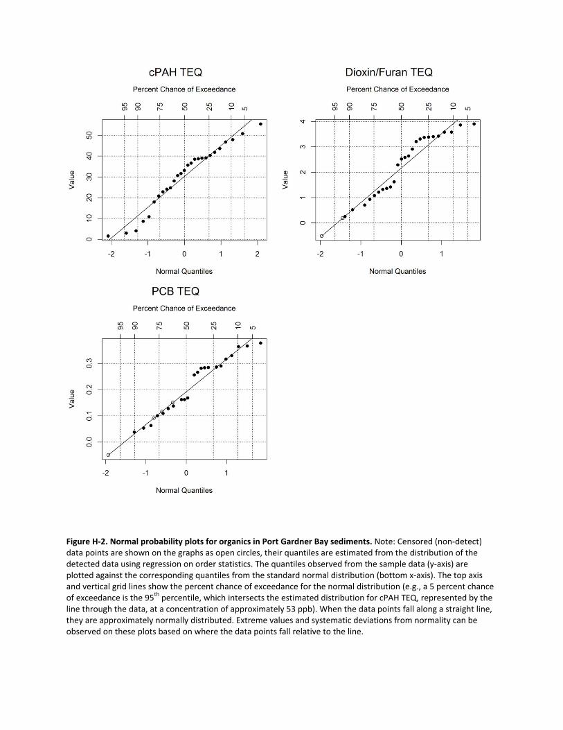
Figure H‐2. Normal probability plots for organics in Port Gardner Bay sediments. Note: Censored (non‐detect) data points are shown on the graphs as open circles, their quantiles are estimated from the distribution of the detected data using regression on order statistics. The quantiles observed from the sample data (y‐axis) are plotted against the corresponding quantiles from the standard normal distribution (bottom x‐axis). The top axis and vertical grid lines show the percent chance of exceedance for the normal distribution (e.g., a 5 percent chance of exceedance is the 95th percentile, which intersects the estimated distribution for cPAH TEQ, represented by the line through the data, at a concentration of approximately 53 ppb). When the data points fall along a straight line, they are approximately normally distributed. Extreme values and systematic deviations from normality can be observed on these plots based on where the data points fall relative to the line.

Figure H‐3. Boxplots showing the distribution of metals concentrations in Port Gardner Bay sediments and Puget Sound natural background (Bold Plus). Note: The 1st, 2nd, and 3rd quartiles are estimated using Kaplan‐Meier for censored data; horizontal lines indicate the level of the highest detection limit. Due to skewness in the cadmium concentrations in the natural background data set, the concentration scale (y‐axis) for cadmium is log‐scaled.

Figure H‐4. Boxplots showing the distribution of organics concentrations in Port Gardner Bay sediments.

Note: The 1st, 2nd, and 3rd quartiles are estimated using Kaplan‐Meier for censored data; horizontal lines indicate the level of the highest detection limit. *The natural background data were incomplete for samples in the Bold Plus data set, so sample sizes for the organic CoCs range from 70 (PCB TEQ) to 91 (dioxin/furan TEQ).

Figure H‐5. Relationship between percent fines and percent total organic carbon in Port Gardner Bay sediments.

Note: The ordinary least squares regression line and its 95 percent confidence interval are shown for these data. Five samples (PG‐34, PG‐51, PG‐53, PG‐60, and PG‐61) are labeled, due to the fact that these samples were identified as unusual by one or more of the methods used in this Appendix H. See text for more details.

Figure H‐6. Relationship between percent fines and each CoC in Port Gardner Bay sediments.

Note: Non‐detected values (turquoise data points) are shown at the reported detection limit. The ordinary least squares regression line is shown for the data in each panel. Five samples (PG‐34, PG‐51, PG‐53, PG‐60, and PG‐61) are labeled, due to the fact that these samples were identified as unusual by one or more of the methods used in this Appendix H. See text for more details.

Figure H‐7. Relationship between percent total organic carbon and each analyte in Port Gardner Bay sediments.

Note: Non‐detected values (turquoise data points) are shown at the reported detection limit. The ordinary least squares regression line is shown for the data in each panel. Five samples (PG‐34, PG‐51, PG‐53, PG‐60, and PG‐61) are labeled, due to the fact that these samples were identified as unusual by one or more of the methods used in this Appendix H. See text for more details.

Figure H‐8. Scatterplot of arsenic versus mercury for a theoretical data set. Note: The centroid is shown as the blue dot, located at the mean concentrations for the two metals. The absolute Euclidean distance from the centroid to Point A (0.3) is smaller but much more unusual than the distance from the centroid to Point B (8.7) due to the direction of covariance/correlation. The Mahalanobis distance is scaled to the covariance and reflects the unexpected result for Point A.

Figure H‐9. QQ‐Plot of the reweighted Mahalanobis squared distances (six CoCs [p = 6]) for the Port Gardner Bay data set. Note: top plot shows the distances for the full dataset (n = 27); bottom plot shows the same data with a truncated y‐axis to illustrate the differences among samples at the lower end of the spectrum (n = 26). Solid horizontal line indicates the threshold for a significant outlier (Sidak adjusted family‐wise type I error rate of 0.05); dashed horizontal line indicates the threshold for outliers at a nominal α (0.05).

Figure H‐10. Principal components analysis (PCA) results for the first two principal components on the combined Port Gardner Bay (n = 27) and Bold (n = 70) data sets, with non‐detects set at the detection limits. The biplot (left) shows both the orientation of the sample points on the first two principal components, and the relationship between the six original chemical variables and these principal components as indicated by the red arrows. The length and direction of a these vectors indicate how the chemical variables are associated with these two principal components. The right plot shows the same orientation of sample points, highlighting the differences between the Port Gardner Bay and Bold data sets.

final data evaluation and summary report

Documents