final analysis of laboratory generated sea waves
TRANSCRIPT
Analysis of Laboratory Generated Sea Waves
Huidong Zhang
M. Sc. Thesis for obtaining the degree of Master of Science in
Naval Architecture and Marine Engineering
Jury
President: Prof. Yordan Garbatov
Supervisor: Prof. Carlos Guedes Soares
Co-Supervisor: Prof. Zhivelina Ivanova Cherneva
Member: Prof. António Alberto Pires Silva
December 2011

Master Thesis Acknowledgements
I
Acknowledgements
This author would like to thank Prof. Carlos Guedes Soares for the general guidance in the
research direction and enough patience to wait for this thesis. The author would also like to
express his great gratitude to Prof. Zhivelina Cherneva who could solve all the author’s problems
and provide a lot of valuable advice throughout the process. Last but not least, the author wants to
give a special thanks to Petya Petrova. Without her help in making MATLAB program, it is not
possible to finish the thesis in such a short time.
Finally, The author would like to thank his family and friends for their understanding and support
in the whole progress of studying abroad.
Huidong Zhang
Lisbon, Portugal
December, 2011
Master Thesis Abstract
II
Abstract
Spectral analysis and statistical analysis are two major methods in analyzing the characteristics of
ocean waves.
In the spectral analysis, both indirect Blackman-Tukey method and direct Cooley-Tukey method
are adopted simultaneously in our work to obtain the wave spectra of wave series in 23 sea states
generated in the laboratory. After comparing the obtained spectra with the standard one proposed
by Goda, and significant wave heights and periods with the corresponding statistical results, it is
drawn that these two methods almost give the same result. Furthermore, some other useful laws
are also summarized at the same time which mainly focus on the spatial variation and relationship
with initial wave steepness for the significant wave height, wave period, spectral moment,
steepness and spectral width parameter.
In the statistical analysis, some relationships about skewness and kurtosis are researched and the
exceedance distributions of wave height, crest and trough in the experiment are compared with
Rayleigh distribution and GC approximation. Typical wave period distributions and joint
distributions in three sea states which are characterized by the initial steepness are also presented
and compared with the theoretical ones. At last, a few characteristics about the maximal wave
height are simply considered in this thesis.
Keywords: surface displacement, wave crest and trough, significant wave height, wave period,
peak frequency, wave basin, wave spectra, spectral moments, Rayleigh distribution, exceedance
distribution, joint distribution of wave period and wave height, maximal wave height.
Master Thesis Resumo
III
Resumo
O análise espectral e análise estatística são os dois métodos principais para a análise das
características das ondas do mar.
Na análise espectral, tanto o método Blackman-Tukey indirecto e método directo Cooley-Tukey
são adoptados simultaneamente no nosso trabalho para obter os espectros de onda da série em 23
estados do mar gerados em laboratório. Depois de comparar os espectros obtidos com o padrão
proposto por Goda, e alturas e períodos com os resultados estatísticos correspondentes, ela é
desenhada que estes dois métodos e quase dão o mesmo resultado. Além disso, algumas outras leis
úteis são também resumidas, ao mesmo tempo que se centram principalmente sobre a variação
espacial e relacionamento com declives na onda inicial para a altura de onda significativa, período
da onda, momento espectral, declive e largura espectral parâmetro.
Na análise estatística, algumas relações sobre assimetria e curtose são pesquisadas e as
distribuições de excedência de altura de onda, crista e calha no experimento são comparados com a
distribuição Rayleigh e aproximação GC. Distribuições de onda típico período e distribuições
conjuntas em três estados do mar, que são caracterizados pela inclinação inicial também são
apresentados e comparados com os teóricos. Por fim, algumas características sobre a altura de
onda máxima são simplesmente considerados nesta tese.
Palavras-chave: deslocamento da superfície, crista da onda e calha, altura de onda
significativa, período de onda, freqüência de pico, onda de bacia, espectros de onda, momentos
espectrais, distribuição de Rayleigh, distribuição de excedência, distribuição conjunta de período
de onda ea altura das ondas, altura de onda máxima.
Master Thesis Contents
IV
Contents
ACKNOWLEDGEMENTS ............................................................................................................................ I
ABSTRACT .............................................................................................................................................. II
RESUMO ............................................................................................................................................... III
CONTENTS ............................................................................................................................................. IV
LIST OF FIGURES .................................................................................................................................... VI
LIST OF TABLES .................................................................................................................................... VIII
CHAPTER 1 INTRODUCTION ............................................................................................................... 1
1.1 MOTIVATION ........................................................................................................................................ 1
1.2 WAVE MEASUREMENT ........................................................................................................................... 2
1.3 SCOPE OF THE PRESENT THESIS ................................................................................................................ 3
CHAPTER 2 BASIC THEORY OF WAVE ANALYSIS ................................................................................... 5
2.1 SPECTRAL ANALYSIS OF SURFACE WAVES .................................................................................................... 5
2.1.1 General ......................................................................................................................................... 5
2.1.2 Sea State Parameters ................................................................................................................... 8
2.1.3 Blackman‐Tukey Method ........................................................................................................... 12
2.1.4 Cooley‐Tukey Method ................................................................................................................. 15
2.2 STATISTICAL ANALYSIS OF SURFACE WAVES ............................................................................................... 19
2.2.1 General ....................................................................................................................................... 19
2.2.2 Surface Displacement ................................................................................................................. 21
2.2.3 Wave Crest and Trough .............................................................................................................. 23
2.2.4 Wave Height ............................................................................................................................... 24
2.2.5 Joint Distribution ........................................................................................................................ 26
CHAPTER 3 EXPERIMENT RESULTS OF WAVE ANALYSIS ...................................................................... 30
3.1 FACILITY AND DATA .............................................................................................................................. 30
3.2 SPECTRAL ANALYSIS ............................................................................................................................. 34
3.2.1 Spectral Comparison .................................................................................................................. 34
3.2.2 Significant Wave Height ............................................................................................................. 37
3.2.3 Wave Period ............................................................................................................................... 40
Master Thesis Contents
V
3.2.4 Zero Spectral Moment and Steepness ........................................................................................ 42
3.2.5 Spectral Width Parameter .......................................................................................................... 44
3.3 STATISTICAL ANALYSIS .......................................................................................................................... 48
3.3.1 Skewness and Kurtosis ............................................................................................................... 48
3.3.2 EDF of Wave Crest Trough and Height ....................................................................................... 51
3.3.3 Wave Period ............................................................................................................................... 55
3.3.4 Joint Distribution ........................................................................................................................ 57
3.3.5 Maximal Wave Height................................................................................................................ 60
3.4 CONCLUSION ...................................................................................................................................... 63
REFERENCE ...................................................................................................................................... 66

Master Thesis List of Figures
VI
List of Figures
Fig. 2.1 Autocorrelation functions .................................................................................................. 15
Fig. 2.2 Error sections in the record of the surface elevation .......................................................... 21
Fig. 2.3 Advantage and disadvantage of filtering wave record ....................................................... 21
Fig. 2.4 three-dimensional and two-dimensional joint distributions in theory for ν=0.1 ................ 29
Fig. 2.5 three-dimensional and two-dimensional joint distributions in theory for ν=0.2 ................ 29
Fig. 2.6 three-dimensional and two-dimensional joint distributions in theory for ν=0.3 ................ 29
Fig. 3.1 Dimensions of offshore basin ............................................................................................ 30
Fig. 3.2 Position of wave gauges .................................................................................................... 30
Fig. 3.3 Time series cut from gauge 1 ............................................................................................. 32
Fig. 3.4 Time series cut from gauge 3 ............................................................................................. 32
Fig. 3.5 Time series cut from gauge 5 ............................................................................................. 32
Fig. 3.6 Wave spectra with initial steepness s0=0.0514 ................................................................... 34
Fig. 3.7 Wave spectra with initial steepness s0=0.1173 ................................................................... 35
Fig. 3.8 Wave spectra with initial steepness s0=0.2084 ................................................................... 35
Fig. 3.9 Normalized wave spectra with initial steepness s0=0.0514 ............................................... 36
Fig. 3.10 Normalized wave spectra with initial steepness s0=0.0879 ............................................. 36
Fig. 3.11 Normalized wave spectra with initial steepness s0=0.1152 .............................................. 37
Fig. 3.12 Normalized wave spectra with initial steepness s0=0.2084 ............................................. 37
Fig. 3.13 Spatial variation of significant wave height in group 1 ................................................... 38
Fig. 3.14 Spatial variation of significant wave height in group 2 ................................................... 39
Fig. 3.15 Spatial variation of significant wave height in group 3 ................................................... 39
Fig. 3.16 Spatial variation of zero-crossing wave period with small initial steepness .................... 40
Fig. 3.17 Spatial variation of zero-crossing wave period with intermediate initial steepness ......... 41
Fig. 3.18 Spatial variation of zero-crossing wave period with large initial steepness ..................... 41
Fig. 3.19 Relationship between relative carrier frequency and initial steepness ............................. 42
Fig. 3.20 Spatial variation of m0 and steepness with small initial steepness .................................. 43
Fig. 3.21 Spatial variation of m0 and steepness with intermediate initial steepness ....................... 43
Fig. 3.22 Spatial variation of m0 and steepness with large initial steepness ................................... 43
Fig. 3.23 Relationship between relative zero spectral moment and initial steepness ...................... 44
Fig. 3.24 Spatial variation of spectral width parameter with small initial steepness ...................... 45
Fig. 3.25 Spatial variation of spectral width parameter with intermediate initial steepness ........... 45
Fig. 3.26 Spatial variation of spectral width parameter with large initial steepness ....................... 46

Master Thesis List of Figures
VII
Fig. 3.27 Relationship between relative spectral width and initial steepness.................................. 46
Fig. 3.28 Distribution of normalized surface displacement in the experiment ................................ 48
Fig. 3.29 Spatial variation of coefficients of skewness and kurtosis in the first test ....................... 49
Fig. 3.30 Spatial variation of coefficients of skewness and kurtosis in the second test .................. 49
Fig. 3.31 Relationship between coefficients of skewness, kurtosis and initial steepness ............... 49
Fig. 3.32 Relationship between coefficient of skewness and wave steepness ................................ 50
Fig. 3.33 Relationship between coefficient of kurtosis and wave steepness ................................... 50
Fig. 3.34 Relationship between coefficient of skewness and kurtosis ............................................ 51
Fig. 3.35 Relationship betweenΛ and appΛ .................................................................................... 52
Fig. 3.36 EDF of wave crest, trough and height for G1 and G3 with small initial steepness ......... 52
Fig. 3.37 EDF of wave crest, trough and height for G4 and G6 with small initial steepness ......... 53
Fig. 3.38 EDF of wave crest, trough and height for G1 and G3 with intermediate initial steepness
................................................................................................................................................. 53
Fig. 3.39 EDF of wave crest, trough and height for G4 and G6 with intermediate initial steepness
................................................................................................................................................. 54
Fig. 3.40 EDF of wave crest, trough and height for G1 and G3 with large initial steepness .......... 54
Fig. 3.41 EDF of wave crest, trough and height for G4 and G6 with large initial steepness .......... 54
Fig. 3.42 Wave period distribution for small wave steepness ......................................................... 56
Fig. 3.43 Wave period distribution for intermediate wave steepness .............................................. 56
Fig. 3.44 Wave period distribution for large wave steepness .......................................................... 56
Fig. 3.45 Joint distribution with small initial wave steepness 1 ...................................................... 58
Fig. 3.46 Joint distribution with small wave steepness 2 ................................................................ 58
Fig. 3.47 Joint distribution with intermediate initial wave steepness 1 ........................................... 58
Fig. 3.48 Joint distribution with intermediate initial wave steepness 2 ........................................... 59
Fig. 3.49 Joint distribution with large initial wave steepness 1 ....................................................... 59
Fig. 3.50 Joint distribution for large initial wave steepness 2 ......................................................... 59
Fig. 3.51 Spatial variation of maximal wave height ........................................................................ 60
Fig. 3.52 Relationship between maximal wave height and the corresponding wave period ........... 61
Fig. 3.53 Relationship between initial steepness and maximal wave steepness .............................. 61

Master Thesis List of Tables
VIII
List of Tables
Table 3.1 Parameters of the wave experiment ................................................................................. 31
Table 3.2 Critical value of initial steepness for the evolution trend of Hs ...................................... 37
Table 3.3 Values of initial steepness for spatial variation ............................................................... 63
Master Thesis Chapter 1 Introduction
1
Chapter 1 Introduction
1.1 Motivation
As soon as people ventured on the sea, waves became important to them. The causes of ocean
waves are various and complicated. In the nature, ocean water is permanently subjected to the
external forces, which dictate what types of waves can be induced in the ocean. Normally, the most
obvious cause of surface waves is an action of wind. As early as 2300 years ago, the ancient
Greeks were well aware of the interaction between the atmosphere and the sea surface. However,
the development of learning about ocean waves was very slow. It was not until into the nineteenth
century that more fundamental knowledge of what caused waves and how they behaved was
accumulated.
Research on ocean waves is really meaningful considering that there are so many fields requiring
wave information. During the World War 2, the requirement to predict wave characteristics for
beach-landing operations generated a major research effort both in the USA and the UK. The
pressure-operated mines which were laid on the sea bed and triggered by the pressure “signature”
of a passing ship must not be triggered by waves.
In the field of coast engineering, waves not only damage breakwaters, but also move sediments.
Taken over long periods of time and considerable stretches of coastline, long-shore drift can fill up
harbors relatively quickly. The interaction of waves with beaches is fascinating but complicated.
The third important application of wave information is ship response to regular and irregular
waves. The pitching and rolling of ships can be very uncomfortable for people. When the motions
get severe, they also slow down the ship, cause cargo to shift, and the associated forces can do
other damage. For warships, it makes it more difficult to operate weapon system accurately, or to
operate aircraft.
Recently, oil companies pay more attention to the forces on the offshore structures which are
Master Thesis Chapter 1 Introduction
2
generated by the ocean waves. In traditional design techniques, the structure is first designed to
withstand the most severe conditions which is likely to meet in 50 or 100 years. However, for
much of the year, it has a significant level of wave activity, and the effects of fatigue must be
allowed for. Thus, as well as an estimate of extreme wave conditions, the statistics of all waves
throughout the year have to be specified. As the development of offshore oil and gas production in
the world, there is a big push for the international companies to gain enough knowledge to ensure
the safety of offshore structures in relation to environment forces.
The last field that will be pointed out is the wave power which is considerable and clean. Wave
power generation will become a widely employed commercial technology in the future.
1.2 Wave Measurement
Normally, the available information on surface waves could be obtained with three methods: field
experiments, laboratory experiments and numerical simulations. In wave experiment under field
conditions, three groups of instruments are used: wave staffs, wave buoys and pressure gauges.
Although field measurement could reflect the wave information directly, it is necessary to consider
the instrument survivability, instrument deployment and retrieval. Moreover, in most cases it is
unavailable to make actual measurements at the site of interest during major storms. Numerical
simulations which include time domain simulation and frequency domain simulation are more and
more concerned by marine engineers and oceanographers due to the interest in directional wave
spectrum. With this method, a lot of money and time could be saved, but there are still some
deviation between simulation and reality which need be further improved.
Laboratory method may be the most common way to obtain the wave information today.
Observations and measurements in laboratory lead to theory being developed to explain it.
Meanwhile, new phenomena predicted by theory lead to experiments being made to verify the
prediction. Thus, discrepancies between theory and measurements stimulate further development
of both. However, correct interpretation of measured results is indeed very difficult. On the one
hand, failure to make correct measurements, or failure to measure the right parameters at the right
spatial location will doom any attempted interpretation for the measurements. On the other hand,
the reliability of laboratory results will depend on the engineer’s understanding of the physical
process as well as the capabilities and limitations of laboratory test equipment and instrumentation.

Master Thesis Chapter 1 Introduction
3
When planning laboratory experiments or model studies, coastal engineers need to know at least
four aspects: the measured physical parameters that could give a meaningful interpretation to the
physical process, the right locations to take measurements, the suitable instruments for the
experiments and the accuracy and reliability of the measurements.
According to different standard, laboratory measurements could be categorized into many different
groups such as geometrical measurements, fluid property measurements, fluid motion
measurements, force and transport measurements and other environmental measurements. The
instruments used to obtain information on surface waves are termed wave gauges which can be
grouped into resistance, capacitance and pressure types. Detailed review of laboratory method
could be found in the book written by Hughes (1993).
1.3 Scope of the Present Thesis
The experiments are carried out in the Technical University of Berlin and the work has been
performed within the project EXTREME SEAS (http://www.mar.ist.utl.pt/extremeseas/), “Design
for Ship Safety in Extreme Seas”, which has been partially financed by the European Union
through its 7th Framework program under contract SCP8-GA-2009-24175.
The job of this thesis is to analyze waves in 23 sea states generated by facility in deep water tank.
The main goal is to investigate and determine the wave parameters which are dependent on the
wave steepness and the distance from the wave maker and to compare the experiment results with
the existed theoretical distributions as well.
In chapter 1, the meaning and motivation of ocean wave research are explained in a brief way from
several perspectives. The methods to obtain wave information are also introduced and mainly
focused on the laboratory experiment.
In chapter 2, the basic theories of wave analysis with spectral method and statistical method are
introduced. In the first section of the theory, besides some concise introductions about sea state
parameters, Blackman-Tukey method and Cooley-Tukey method are explained briefly. In the
second section of the theory, the theoretical distribution models of surface displacement, wave
crest, wave trough, wave period, etc. are described in few words.

Master Thesis Chapter 1 Introduction
4
In chapter 3, in the spectral analysis, the wave spectra are investigated with direct and indirect
methods. The spatial variation of some wave parameters and their relationship with the initial
wave steepness are also researched. In the statistical analysis, the observed distributions of wave
surface displacement crest, trough and height and so on are compared with the theoretical models
and meanwhile the dependence with nonlinearity is also considered .At last, some conclusions are
summarized together and the future work is proposed.
.
Master Thesis Chapter 2 Basic Theory of Wave Analysis
5
Chapter 2 Basic Theory of Wave Analysis
2.1 Spectral Analysis of Surface Waves
2.1.1 General
The waves on the sea surface are not simple sinusoids. They usually exhibit irregular profiles
randomly changing in space and time. In order to describe the characteristics of this random
phenomenon clearly, the concept of stochastic process is introduced. Furthermore, the probabilistic
principles can be used to find the most favorable marginal and joint probabilistic laws applicable
to the desired wave properties: periods, crests, heights, etc...
The stochastic approach spans three domains: time, frequency and probability. Usually, the
derivation of the probability law requires several simplifying assumptions. The statistical
properties of stochastic process are evaluated based on an ensemble, and hence they may or may
not be the same as time progresses. The condition for a stationary stochastic process requires that
the joint distribution be invariant irrespective of time, which is somewhat severe in practice. A
more relaxed condition that is commonly acknowledged called weakly stationary with zero mean
is taken in the analysis of ocean surface waves.
Another very important assumption for the analysis of ocean waves is ergodic process. It is
developed by statisticians with the conditions under which the time average of a single record
(sample mean) is equivalent to the ensemble average. It is taken for granted that the ergodic
property holds for stochastic processes. Therefore, the wave surface displacement pertained to a
single record can be used to instead of an ensemble of data.
Narrow-banded which implies that the amplitude and phase of the process vary slowly and
randomly with time while the frequency retains a constant value is also assumed in the analysis of
continuous-state and continuous-time stochastic processes. In other words, the distribution of wave
energy in the frequency domain is concentrated around some characteristic value, the mode of the
frequency.

Master Thesis Chapter 2 Basic Theory of Wave Analysis
6
Based on the assumptions mentioned above, the function of wave spectra can be deduced and
some useful parameters could be determined. The weak stationarity, also known as the covariance
stationarity, suggests that the mean of the process are constant independent of time and the
autocovariance function of the process depends only on the time-lag for all time.
Let ( )x t represents the free surface elevation oscillating around the mean water level. Then, the
weak stationarity will be expressed as:
[ ]( )E x t x const= = (2.1)
[ ] 2 2var ( ) ( ( ) )x t E x t x constσ⎡ ⎤= − = =⎣ ⎦ (2.2)
1 2 1 2 1 2cov[ ( ), ( )] [( ( ) )( ( ) )] ( , ) ( )x t x t E x t x t B t t Bμ μ τ= − − = = (2.3)
where [ ]E stands for the statistical expectation; 2 1t tτ = − is the time lag; ( )B τ is the
autocovariance, the second order joint central moment of the process.
Similarly to ( )B τ , the second ordinary joint spectral moment, called the autocorrelation function,
can be defined as:
[ ] [ ]1 2 1 2 1 2( ), ( ) ( ) ( ) ( , ) ( )cor x t x t E x t x t R t t R τ= = = (2.4)
The definition in Eq.(2.4) implies that ( )R τ is identical to ( )B τ when the process has zero-mean,
that is 0x = .
It is necessary to point out that according to the mathematical definitions, these statistical variables
mentioned above should be calculated on the basis of the ensemble of the wave records,
{ ( ) }, 1,...iX x t i n= = , given n →∞ . However, for example, gathering data simultaneously at
different points of space covered by the storm is a difficult and almost impossible task. Under the
assumption of being weakly stationary and ergodic, it is possible to substitute the ensemble with a
single record at a fixed point in space. The single sample in this case becomes representative for
the wave population, irrespective of the wave directionality.
The autocorrelation function gives important information in the stochastic analysis for conversion
from the time domain to the frequency domain. For convenience, it is assumed that the Fourier
transform of a random process exists over the entire time domain and the truncated function is also

Master Thesis Chapter 2 Basic Theory of Wave Analysis
7
considered in the analysis. After that, it is possible to find the spectral density function ( )S ω from
the known autocorrelation function ( )R τ by means of the Wiener-Khintchine theorem. The
Wiener-Khintchine theorem represents ( )R τ and ( )S ω as a pair of Fourier transforms.
0
1 1( ) ( ) ( )cos2
iS R e d R dωτω τ τ τ ωτ τπ π
+∞ +∞−
−∞= =∫ ∫ (2.5)
0
( ) ( ) 2 ( )cosiR S e d S dωττ ω ω ω ωτ ω+∞ +∞+
−∞= =∫ ∫ (2.6)
Eq. (2.6) shows the most important property of ( )S ω for 0τ = .
(0) ( )R S dω ω+∞
−∞= ∫ (2.7)
According to the definition of ( )R τ in Eq.(2.4), it results in the equation known as the Parseval
theorem, i.e.
2( ) ( )E x t S dω ω+∞
−∞⎡ ⎤ =⎣ ⎦ ∫ (2.8)
The Parseval theorem specifies the relationship between the wave energy (the variance) of the
process estimated in the time domain (left-handed side of the equation) and the wave energy in the
frequency domain (right-handed side of the equation).
In order to make the above theorem clearly, we measure the elevation of the sea surface at the
origin of the coordinate system (which can be done without loss of generality), then wave profile
will become:
( ) cos( )n n nn
x t a tω θ= +∑ (2.9)
Then
2 ( ) cos( ) cos( )n m n n m mn m
x t a a t tω θ ω θ= + +∑∑ (2.10)
After some computation of trigonometric function, and taking a long-term average, it gives:
2 21( )2 n
nE x t a⎡ ⎤ =⎣ ⎦ ∑ (2.11)
Now with the help of Eq.(2.8), Eq.(2.11), it is much easier to understand that the area under the
wave spectrum is equal to the wave energy. ( )S ω is usually abbreviated to “the omnidirectional
spectrum” or sometimes “the point spectrum”. It is also common practice to refer to it as “the
wave energy spectrum”, but strictly speaking, the energy spectrum would be:
Master Thesis Chapter 2 Basic Theory of Wave Analysis
8
( ) ( )E gSω ρ ω= (2.12)
2.1.2 Sea State Parameters
In the early days of the modern approach, the parameters could only be determined directly from
the time-histories which is now known as deterministic analysis. As the development of digital
computers, spectral analysis by analogue method now becomes more convenient and more reliable.
In the frequency domain, the spectral density function can be described in terms of its moments.
The ordinary spectral moments are determined by the integral:
*
0( )n
nm S dω ω ω+∞
= ∫ (2.13)
In particular, the zeroth-order spectral moment 0m (the area under the spectral density curve)
represents the variance of the surface elevation process. It is also representative for the total energy
of the waves as mentioned above. The second-order spectral moment represents the variance of the
wave elevation velocity and the fourth-order spectral moment represents the variance of the wave
elevation acceleration.
A measurement which is frequently used in the statistical analysis of wave data is the significant
wave height. The significant wave height is a characteristic measurement that defines the level of
severity of the given sea state. According to the statistical definition, it equals the average of
one-third of the largest waves in a sample of wave heights, or the average of the largest waves
having probability of exceedance 1/3. This wave height, 1/ 3H should be close to the average wave
detected visually at sea.
The second definition of significant wave height, more frequently used in Gaussian sea, is based
on the information from the wave spectrum.
0 04.004mH m= (2.14)
For a narrowband spectrum it is expected that 0 1/3mH H≈ , However, normally for the typical sea
state, 0 1/3 00.9 m mH H H< < . Analysis of full-scale data shows that the spectral definition
overestimates by approximately 5% the statistical formulation.
The peak period of the spectrum pT corresponds to the frequency at the mode of the spectral
Master Thesis Chapter 2 Basic Theory of Wave Analysis
9
density, the peak frequency, pω :
2
pp
T πω
= (2.15)
Moreover, some characteristic wave frequencies and periods can be derived from the ordinary
spectral moments. The mean spectral frequency (also could be defined as carrier wave frequency)
and the associated mean spectral period are expressed as:
101
0
mm
ω = (2.16)
001
01 1
2 2 mTm
π πω
= = (2.17)
The average zero-up-crossing angular wave frequency and the associated average zero-up-crossing
period are given as:
2
0z
mm
ω = (2.18)
0
2
2 2zz
mTm
π πω
= = (2.19)
The crest period or the average period between wave crests is represented by:
2
4
2cmTm
π= (2.20)
Another very important measure of the distribution of the frequency components in the sea state is
the spectral bandwidth. Several measures of the width of the spectrum have been defined and used
to validate the assumption of narrow spectrum. One of the parameters commonly used is proposed
by Longuet-Higgins (1975), the spectral width parameter:
1/ 2
0 221
1m mm
ν⎛ ⎞
= −⎜ ⎟⎝ ⎠
(2.21)
which represents the normalized radius of gyration of the spectrum about the mean frequency 01ω .
For describing its derivation, it is convenient to think in mechanical terms. The moment of inertia
about the axis 0ω = is 2m . The moment of inertia about the mean frequency 01ω obtained in
Eq.(2.16), that is, about the centre of gravity, is 22 01 0m mω− . The radius of gyration about the mean
frequency is:

Master Thesis Chapter 2 Basic Theory of Wave Analysis
10
1/ 2 1/ 22
22 01 0 201
0 0
m m mm mω ω
⎛ ⎞ ⎛ ⎞−= −⎜ ⎟ ⎜ ⎟
⎝ ⎠ ⎝ ⎠ (2.22)
Normalizing Eq.(2.22) with the mean frequency 01ω , Eq.(2.21) will be obtained. For a spectrum of
narrow bandwidth, 0ν → . For example, for the Pierson-Moskowitz spectrum, 0.425ν = ; for
JONSWAP spectrum with 3.3γ = , 0.7aσ = , 0.9bσ = , 0.390ν = . The irregularity of the wave
field is reflected in the large estimates ofν . Another parameter is the bandwidth parameter of
Cartwright and Longuet-Higgins (1956):
1/ 22
2
0 4
1 mm m
ε⎛ ⎞
= −⎜ ⎟⎝ ⎠
(2.23)
Again, for a narrowband spectrum, it is expected that 0ε → . Since this parameter depends on the
magnitude of the fourth-order spectral moment, 4m , instead of representing the energy distribution
over the entire frequency range, it only represents the range of frequencies where the dominant
energy exists. Because of this reason, it is rarely used recently.
The last very useful measure for a random sea is the steepness which is defined:
2
02
2 mp
p
HSgTπ
= (2.24)
It has no precise physical meaning. But by analogy with the case of the periodic wave, it can be
considered as the steepness of the sea.
So far, there are several expressions used as standard forms of the frequency spectrum which can
be regarded as having been derived empirically with some theoretical guidance. Probably the most
popular spectrum among all proposed forms is that proposed by Pierson and Moskowitz (1964),
who using the field data and theoretical discoveries of Phillips (1958), showed that:
4
2 5( ) exp gS g BU
ω α ωω
−⎡ ⎤⎛ ⎞= −⎢ ⎥⎜ ⎟
⎝ ⎠⎢ ⎥⎣ ⎦ (2.25)
where 0.0081α = , 0.74B = and U is a wind speed at an elevation of 19.5m above the sea surface.
The shape of the wave spectrum is controlled by a single parameter, wind speed U . The spectrum
of Eq.(2.25) was proposed for fully-developed sea, when phase speed is equal to wind speed. The
experimental spectra given by Pierson and Moskowitz yields
Master Thesis Chapter 2 Basic Theory of Wave Analysis
11
4
2 5 5( ) exp4 p
S g ωω α ωω
−
−⎡ ⎤⎛ ⎞⎢ ⎥= − ⎜ ⎟⎜ ⎟⎢ ⎥⎝ ⎠⎣ ⎦
(2.26)
Some mathematical problems arise when calculating the fourth order spectral moment using
Eq.(2.26).This moment, which physically denotes the mean-squared acceleration measured at a
Eulerian point, is unbounded.
Later, the JONSWAP spectrum extends the Pierson-Moskowitz spectrum to including fetch-limited
seas. This spectrum is based on an extensive wave measurement program (Joint North Sea Wave
Project) carried out in 1968 and 1969 in the North Sea. The JONSWAP spectrum, after publication
in 1973, received almost instant recognition and became very well known in international
literature. The resulting spectral model is taken as the following form (Hasselmann et al.,1973):
4
2 5 5( ) exp4 p
S g δωω α ω γω
−
−⎡ ⎤⎛ ⎞⎢ ⎥= − ⎜ ⎟⎜ ⎟⎢ ⎥⎝ ⎠⎣ ⎦
(2.27)
where2
2 20
( )exp
2p
p
ω ωδ
σ ω⎡ ⎤−
= −⎢ ⎥⎢ ⎥⎣ ⎦
.
Spectrum (2.27) contains five parameters which should be known:α , the Phillips’s constant,
limited by the value 0.0081 in the case of the Pierson-Moskowitz spectrum for fully-developed
seas; pω , the spectral peak frequency; 0 0.07aσ σ= = for pω ω< and 0 0.09bσ σ= = for pω ω> ;
γ the peak enhancement parameter that describes the degree of peakedness of the spectrum.
The term δγ is the peak enhancement factor, added to the Pierson-Moskowitz formulation in order
to represent a narrower and more peaked spectrum which is typical for growing seas. Also,γ is a
random Gaussian variable with mean 3.3 and variance 0.62, such that 3.3γ = represents the mean
JONSWAP spectrum and 1γ = represents the Pierson-Moskowitz spectrum. The width of the
enhancement at the peak region is given by the values of 0σ . The values ofα andγ depend on the
stage of development of the sea.
The alternative formulation of JONSWAP as a function of the significant wave height and peak
frequency was proposed by Goda (1988):

Master Thesis Chapter 2 Basic Theory of Wave Analysis
12
45
* 24
5( ) exp4p p
sS H δω ωω α γω ω
−−
−
⎡ ⎤⎛ ⎞⎢ ⎥= − ⎜ ⎟⎜ ⎟⎢ ⎥⎝ ⎠⎣ ⎦
(2.28)
where
* *0.06240.1850.23 0.0336
1.9
α βγ
γ
=⎡ ⎤
+ −⎢ ⎥+⎣ ⎦
* 1.094 0.01915lnβ γ= − .
The standard formulations in Eq.(2.27) and Eq.(2.28) can be fitted by the measured data. For
example, the values of the significant wave height, peak period and peak factor used in Eq.(2.28)
can be found with the best fit minimizing the sum of squared differences between the smoothed
measured spectrum and the JONSWAP standard formula in Eq.(2.28). As another option to fit the
measured data with the standard JONSWAP formula is to use the Günter method which is given in
detail in Tucker and Pitt (2001). The logic of this method is clear and simple while the values of
parameters computed tends to deviate from the normal ones.
2.1.3 Blackman-Tukey Method
The method proposed by Blackman and Tukey (1959) for the estimation of the wave spectrum is
based on the Wiener-Khintchine theorem. The Blackman-Tukey procedure, also known as the
method of correlogram is an indirect method, since first it requires estimation of the
autocorrelation function and then applies the Fourier transform to it. The procedure is described in
Massel (1996) and it will be repeated briefly below.
a) Transformation of variables
Let the surface elevation process is ( )x t . The total duration of wave recordings isT N t= Δ , where
N is the number of the sampled data and tΔ [s] is the constant interval of data sampling. A new
time series ix , with zero-mean and unit standard deviation could be obtained:
ii
x xxσ−
= (2.29)
b) Estimation of the autocorrelation function
The autocorrelation function, ( )R τ , is directly obtained from the time series, by computing a set
Master Thesis Chapter 2 Basic Theory of Wave Analysis
13
of average products among the sample data values. One of the possible estimators for ( )R τ is
expressed as:
1
1( ) , 0,1, 2,...,N r
n n rn
R r t x x r mN r
−
+
=
Δ = =− ∑ (2.30)
where r stands for the lag number; m is the maximum lag number ( m N ). Selection of the m
value, which provides the optimum estimate for the autocorrelation function, is also very
important. The finite value of m implies that the surface elevations at large time t m t> Δ are
uncorrelated.
c) Suppression of the spectral energy leakage
A window should be used for the autocorrelation function to suppress the spectrum energy leakage.
The window aims at tapering the autocorrelation function, so as to eliminate the discontinuity at
the end of ( )R τ . There are numerous such windows in use. A typical window is the cosine
Hanning window:
1 1 cos , 0,1, 2,...
( ) 20 ,
h
r for r mu r t m
for r m
π⎧ ⎛ ⎞+ =⎪ ⎜ ⎟Δ = ⎝ ⎠⎨⎪ >⎩
(2.31)
Applying the filter in Eq.(2.31) to the autocorrelation function, the latter is recalculated as:
( ) ( ) ( )hR r t R r t u r tΔ = Δ Δ (2.32)
d) Calculation of the frequency spectral density
The spectral density is calculated by numerical integration from the Wiener-Khintchine equations
in Eq.(2.5):
( ) ( ) ( ) ( )1
1
( ) 0 2 cos cosm
kr
t rkS R R r t R m t kmπω π
π
−
=
Δ ⎧ ⎫⎛ ⎞= + Δ + Δ⎨ ⎬⎜ ⎟⎝ ⎠⎩ ⎭
∑ (2.33)
where t dtΔ = in the Wiener-Khintchine integral. The frequencyω [rad/s] corresponding to each
time-lag is expressed as:
, 0,1, 2,...,kkk k m
m tπω ω= Δ = =Δ
(2.34)
The fundamental increment tΔ , also named Nyquist sampling interval, is the maximum interval
required to properly describe the data ( )x t . According to the Nyquist frequency, the maximum
Master Thesis Chapter 2 Basic Theory of Wave Analysis
14
useful frequency in the spectrum is given by:
max N tπω ω= =Δ
(2.35)
The spectral estimate in Eq.(2.33) describes the mean square value2
( )x t⎡ ⎤⎣ ⎦ in terms of frequency
components laying inside the frequency band ( ) ( ){ }2 , 2e eB Bω ω− + , where ( )2eB m tπ= Δ
[rad/s] is the obtained frequency resolution for the chosen sampling interval tΔ . Eq.(2.33) gives
2m independent estimates of the spectrum for the reason that the estimates separated by
frequency increments smaller than 2 N mω are correlated. For a given bandwidth eB , the required
maximum lag number m can be determined as:
2
e
mB tπ
=Δ
(2.36)
e) Smoothing of the spectral estimate
The spectral estimation in Eq.(2.33) exhibits large variance, so it becomes necessary to smooth it
in order to reduce the statistical variability. This can be done by simple block-averaging,
moving-average or by means of weighted averaging. The simple moving average method is
expressed by:
( ) ( ) ( )12 1
p
k k jj p
S Sp
ω ω +=−
=+ ∑ (2.37)
where ( )kS ω is the smoothed spectrum resulting from averaging of ( )kS ω over ( )2 1p +
neighboring values.
In order to further increase the estimate accuracy, some techniques should be used and the
maximal lag number needs to be selected carefully in the procedure. The method taken in this
thesis for the maximum lag is to find the envelope of the autocorrelation function and then to
choose the lag at the position where the envelope reaches its first minimum as shown in Fig. 2.1.

Master Thesis Chapter 2 Basic Theory of Wave Analysis
15
Fig. 2.1 Autocorrelation functions
2.1.4 Cooley-Tukey Method
An alternative method, known as Cooley-Tukey method applies direct Fast Fourier Transform to
the water surface displacements and is basically used lately as a result of saving a lot of
computational time. In the following part, some critical procedures in this method are briefly
explained.
a) Data preprocessing
As mentioned in step 1 of Blackman-Tukey method, a mean value from the digital data needs to be
subtracted. Trend removing and filtering will be processed if they are necessary.
b) Window function selection
In signal processing, there are two bothering problems: the first one is that the signal can only be
measured for a limited time which means nothing could be known about the behavior outside the
measurement interval; the second one is that Fast Fourier Transform is base on the fact that the
signal is periodic which is not true in reality. When the FFT assumes the signal repeats, it will
assume discontinuities that are not really there. Therefore, the spectral leakage will happen. In
order to obtain the periodic signal, the procedure is to multiply the signal within the measurement
time by some function that smoothly reduces the signal to zero at the end point. One of the simple
and useful window functions is Hanning window which should be applied first before FFT. It is
expressed in the following formula:

Master Thesis Chapter 2 Basic Theory of Wave Analysis
16
i i ix x w= ⋅ (2.38)
The Hanning window is defined as follows:
( )2 11 1 cos ; 1...
2i
iw i N
Nπ⎡ ⎤⋅ −⎛ ⎞
= − =⎢ ⎥⎜ ⎟⎢ ⎥⎝ ⎠⎣ ⎦
(2.39)
c) Fast Fourier Transform
The fast Fourier Transform is a DFT with special algorithm developed by Tukey and Cooley (1965)
which reduces the number of computations from something on the order of 2N to ( )logN N .
Although many variants of the FFT algorithm (Oran, 1974) exist, but the critical parts of this
algorithm do not change.
Bit reversed indexing
It is a good choice to reverse the bits of binary representation of i to get the corresponding
array index for the input “time domain” data at the initial stage of the program. Therefore, the
output result will be in the normal order.
Nested loops instead of recursive decimation in time
Three nested loops should be included in the program.
Pass Loop: the outer loop, an 2pN = point transform will perform p ”passes”, indexed by
1,2,...,l p= ;
Block Loop: the inner loop, each pass l has 2 p l− sub-blocks whose size is 2l , indexed by
1, 2,..., 2 p lm −= ;
Butterfly Loop: the middle loop, each sub-block operation will perform 12l− butterflies,
indexed by 11, 2,..., 2ln −= ;
Twiddle factor tricks
In order to avoid the time-consuming work of computing sinusoidal function and cosine
function for every butterfly. In the program, it is convenient to set the step size of twiddle
factor as 2lW . Therefore, the twiddle factors used in each pass should be 12
nlW − , where the term
( )exp 2NW j Nπ= .
Master Thesis Chapter 2 Basic Theory of Wave Analysis
17
Because the input data ix are always real, after fast Fourier transform, the output array iX obeys the
following relationship:
*2 , 2,3,..., 2N i iX X i N− + = = (2.40)
where*denotes complex conjugation. Since N is also even, 1X and 2 1NX + are both real. Thus, only
the first 2 1N + distinct real and complex numbers which should be expressed in the form of
square of absolute value would be useful in the spectrum analysis. These correspond to the
frequencies:
( )1 , 1,2,..., 2 1i i i Nω ω= − Δ = + (2.41)
where the width of a frequency bin is given by
2
N tπωΔ =Δ
(2.42)
The apparent loss of information is explained by the fact that the output consists of complex
numbers while the input is real.
d) Averaging and overlap
If we just compute one estimate of a spectrum with the first three steps described so far, it will be
found that the result is rather variant. It does not help to increase the length N of the FFT and that
only reduces the width of frequency bin without impairing the variance.
The practical remedy is to take the average of k estimates and hence reduce the standard
deviation of the averaged result by a factor of 1 k . However, the precondition is that the
properties of the signal must remain stationary during the average. Thus, it is necessary to select a
suitable value for the length N of the FFT. In conjunction with the use of window functions, this
method of averaging several spectra is known as “Welch’s Overlapped Segmented Average”.
If the original data is split up into several non-overlapping segments of length N and each segment
is processed by a FFT with a window function, some information may be ignored in the analysis
due to the fact that the window function is typically very small or zero near its boundaries. It is
clearly not very good in some situations such as the maximal possible wave height is to be
extracted from it. This situation could be improved by letting the segments overlap. Normally,
different windows need different overlapped segments. For Hanning window which is relatively
Master Thesis Chapter 2 Basic Theory of Wave Analysis
18
wide in the time domain, 50% is a commonly recommended. For narrower window such as
flat-top window, a higher overlap up to 84% may be appropriate. On the other hand, if the overlap
becomes too big, the spectrum estimates from subsequent stretches become strongly correlated,
even if the signal is random. What is worse, it will waste computational efforts.
Sometimes, the confident interval would be used in the estimate. Just keep one thing in mind,
when the overlapping is zero, confident interval will be needed and 95% is the recommend value
in the engineering project.
e) Scaling the result
Now it is time to normalize the results of the FFT. Based on what has been mentioned above and
the use of window function, a new normalized parameter is needed to instead of N :
22
1
N
ii
B w=
= ∑ (2.43)
The power spectral density could be obtained in the following form:
( ) 2
12 max
1 , 1,2,..., 2 1k
i ijj
S X i NkB
ωω =
= = +∑ (2.44)
The factor k comes from the fact that k segments have been summed up together during the whole
process.
f) Smoothing of spectral estimation and Parameters Selection
If a smoothed spectral is needed, the same procedure in step 6 of Blackman-Tukey Method could
be taken and will not be repeated here again.

Master Thesis Chapter 2 Basic Theory of Wave Analysis
19
2.2 Statistical Analysis of Surface Waves
2.2.1 General
Besides the spectral analysis of the ocean surface waves, the statistical distribution of waves are
also very useful in the wave research, especially in ocean engineering. For example, the statistics
of extreme waves plays a very important role in the determination of the design wave height for
offshore and costal structures. In the statistical analysis, wave parameters such as wave height and
wave period are considered as random variables with statistical characteristics.
Normally, the statistics of ocean waves will be considered in a short-term and long-term scale. In
the following parts of this chapter, the short-term statistics based on the Gaussian processes will be
discussed for the distribution of surface displacement. The theoretical distributions of wave height,
crest, trough and wave period are also briefly introduced.
Firstly, it is necessary to explain the thorough procedure for finding the zero-up-crossing points,
wave maxima, wave minima and some practical problems in application.
The points of zero-up crossing of the wave profile are determined by the following criteria:
1
1
0
0i i
i
x x
x+
+
⎧ <⎪⎨
>⎪⎩ (2.45)
where ix denotes the -thi data point of the surface elevation obtained from Eq.(2.29). Then, the
time of the zero-up-crossing is found by linear interpolation between the sampling time of ix and
1ix + . The time difference between one zero-up-crossing point and the successive one in the same
direction gives the zero-up-crossing wave period. The global maximum surface elevation is
defined as the wave crest between two consecutive zero-up-crossing points where
1
1
i i
i i
x x
x x−
+
⎧ <⎪⎨
>⎪⎩ (2.46)
It is suggested that the time and the magnitude of the maximum point should be estimated by
fitting three consecutive points 1ix − , ix and 1ix + with a parabolic equation to avoid the possibility of
underestimating the true maximum value among those discrete sampling points. The parabolic
fitting is given by:
Master Thesis Chapter 2 Basic Theory of Wave Analysis
20
2
max4Bx D
A= − (2.47)
max 2itBt tA
Δ= − (2.48)
where tΔ is the time sampling interval and
( )( )1 12
1 22
i i iA x x xt
− += − +Δ
(2.49)
( )1 11
2 i iB x xt + −= −
Δ (2.50)
iD x= (2.51)
The global minimum wave profile between two consecutive zero-up-crossing points is defined as
the wave trough which is determined in the same procedure as wave crest. And the only difference
is the requirement:
1
1
i i
i i
x x
x x−
+
⎧ >⎪⎨
<⎪⎩ (2.52)
The wave height is defined by the difference between the crest and wave trough in a given wave
cycle.
Sometimes due to the very small time interval and the problem of equipment, the recorded wave
elevation may fluctuate around the mean water lever. It satisfies Eq.(2.45) but is not the desired
point. As a result, the obtained probability of small wave height and wave period will be enlarged.
Therefore, it is necessary to make full use of some techniques to solve this problem such as
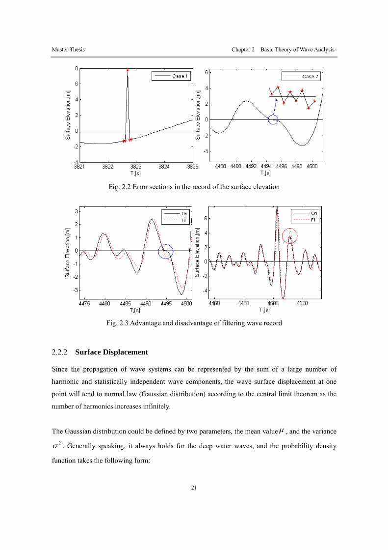
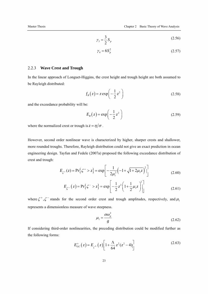
filtering wave data at the beginning or adding more conditions in Eq.(2.45).
For example (see Fig. 2.2), the conditions described in Eq.(2.45) will result in some errors in the
statistical analysis. Fortunately, some functions in MATLAB could be used to filter the undesired
high frequency and low frequency parts in the wave record. However, as shown in Fig. 2.3,
although the error record could be eliminated, some other errors will be induced inevitably due to
the missed information such as the wave height..
Master Thesis Chapter 2 Basic Theory of Wave Analysis
21
Fig. 2.2 Error sections in the record of the surface elevation
Fig. 2.3 Advantage and disadvantage of filtering wave record
2.2.2 Surface Displacement
Since the propagation of wave systems can be represented by the sum of a large number of
harmonic and statistically independent wave components, the wave surface displacement at one
point will tend to normal law (Gaussian distribution) according to the central limit theorem as the
number of harmonics increases infinitely.
The Gaussian distribution could be defined by two parameters, the mean valueμ , and the variance2σ . Generally speaking, it always holds for the deep water waves, and the probability density
function takes the following form:

Master Thesis Chapter 2 Basic Theory of Wave Analysis
22
( ) ( )2
2
1 exp ,22
xf x x
μσπσ
⎡ ⎤−= − −∞ < < +∞⎢ ⎥
⎢ ⎥⎣ ⎦ (2.53)
The mean and variance are equal to the first-order and second-order cumulants respectively, or the
corresponding central moments if the mean is zero.
In most cases, although the distribution of surface displacement is approximately Gaussian, a
small asymmetry and different peakedness are observed. These deviations from the Gaussian
distribution can be expressed in two parameters, coefficients of skewness 3γ and kurtosis 4γ , which
are higher order quantities and related to the nonlinearities in the wave basin.
3 33 3 2 3
2
κ κγκ σ
= = (2.54)
4 44 2 4
2
κ κγκ σ
= = (2.55)
where 2κ , 3κ and 4κ represent second-order, third-order and fourth-order cumulants respectively.
Thus Eq.(2.54) and Eq.(2.55) also represent the normalized third-order and fourth-order cumulants
respectively. Only when coefficients of skewness and kurtosis are both equal to zero at the same
time, the random variable is normally distributed.
The coefficient of skewness measures the steepness in the wave basin or the vertical asymmetry in
the wave profile provoked by second-order effects and is exemplified by the sharp crests and
rounded troughs of gravity waves. The positive coefficient of skewness will mean a bigger
probability of occurrence of large crests and that the empirical distribution will be skewed to the
right with respect to the mode of the Gaussian distribution, such that the mode of the distribution is
located at a value smaller than the mean. On the other hand, although coefficient of kurtosis is
more commonly defined as the fourth cumulants divided by the square of the second cumulants, it
is equal to the fourth order central moment divided by the square of the probability distribution
minus 3. The positive coefficient of kurtosis reflects the total increase of crest-to-trough wave
height, due to third order nonlinear interactions.
For a narrow band unidirectional weakly nonlinear train up to second order, the coefficients of
skewness and kurtosis are related to the steepness pS in Eq.(2.24) (Mori and Janssen, 2006)
Master Thesis Chapter 2 Basic Theory of Wave Analysis
23
3
32 pSγ = (2.56)
24 6 pSγ = (2.57)
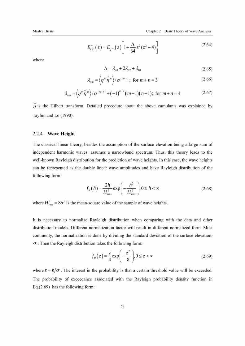
2.2.3 Wave Crest and Trough
In the linear approach of Longuet-Higgins, the crest height and trough height are both assumed to
be Rayleigh distributed:
( ) 21exp2Rf z z z⎛ ⎞= −⎜ ⎟
⎝ ⎠ (2.58)
and the exceedance probability will be:
( ) 21exp2RE z z⎛ ⎞= −⎜ ⎟
⎝ ⎠ (2.59)
where the normalized crest or trough is z η σ= .
However, second order nonlinear wave is characterized by higher, sharper crests and shallower,
more rounded troughs. Therefore, Rayleigh distribution could not give an exact prediction in ocean
engineering design. Tayfun and Fedele (2007a) proposed the following exceedance distribution of
crest and trough:
{ } ( )2
121
1( ) Pr exp 1 1 22
E z z zζ ζ μμ+
+ ⎡ ⎤= > = − − + +⎢ ⎥
⎣ ⎦ (2.60)
( ) { }2
21
1 1Pr exp 12 2
E z z z zζ ζ μ−−
⎡ ⎤⎛ ⎞= > = − +⎢ ⎥⎜ ⎟⎝ ⎠⎢ ⎥⎣ ⎦
(2.61)
where ,ζ ζ+ − stands for the second order crest and trough amplitudes, respectively, and 1μ
represents a dimensionless measure of wave steepness.
2
1p
gσω
μ = (2.62)
If considering third-order nonlinearities, the preceding distribution could be modified further as
the following forms:
( ) ( ) 2 21 ( 4)64GCE z E z z z
ζ+
+Λ⎡ ⎤= + −⎢ ⎥⎣ ⎦
(2.63)
Master Thesis Chapter 2 Basic Theory of Wave Analysis
24
( ) ( ) 2 21 ( 4)64GCE z E z z z
ζ−
−Λ⎡ ⎤= + −⎢ ⎥⎣ ⎦
(2.64)
where
40 22 042λ λ λΛ = + + (2.65)
( )/ ; for 3m n m nnm m nλ η η σ += + = (2.66)
( ) ( )( )/ 2( )/ 1 1 1 ; for 4mm n m nnm m n m nλ η η σ += + − − − + = (2.67)
η is the Hilbert transform. Detailed procedure about the above cumulants was explained by
Tayfun and Lo (1990).
2.2.4 Wave Height
The classical linear theory, besides the assumption of the surface elevation being a large sum of
independent harmonic waves, assumes a narrowband spectrum. Thus, this theory leads to the
well-known Rayleigh distribution for the prediction of wave heights. In this case, the wave heights
can be represented as the double linear wave amplitudes and have Rayleigh distribution of the
following form:
( )2
2 2
2 exp ,0Rrms rms
h hf h hH H
⎛ ⎞= − ≤ < ∞⎜ ⎟
⎝ ⎠ (2.68)
where 2 28rmsH σ= is the mean-square value of the sample of wave heights.
It is necessary to normalize Rayleigh distribution when comparing with the data and other
distribution models. Different normalization factor will result in different normalized form. Most
commonly, the normalization is done by dividing the standard deviation of the surface elevation,σ . Then the Rayleigh distribution takes the following form:
( )2
exp ,04 8Rz zf z z
⎛ ⎞= − ≤ < ∞⎜ ⎟
⎝ ⎠ (2.69)
where z h σ= . The interest in the probability is that a certain threshold value will be exceeded.
The probability of exceedance associated with the Rayleigh probability density function in
Eq.(2.69) has the following form:

Master Thesis Chapter 2 Basic Theory of Wave Analysis
25
( ) ( )2
Pr exp ,08RzE z H z zσ
⎛ ⎞= > = − ≤ < ∞⎜ ⎟
⎝ ⎠ (2.70)
However, it has been reported that Rayleigh exceedance distribution tends to overestimate the
crest-to-trough heights of large waves by about 7%-8% (Tayfun and Fedele, 2007a). This
discrepancy has been found to be mainly caused by the assumption in the Rayleigh theory of the
wave height being double the crest height.
Therefore, some more advanced theories have been presented in the present study. Tayfun and
Fedele (2007a) presented the third-order approximations of wave heights based on the
Gram-Charlier (GC) expansions:
( ) ( ) ( )4 21 32 1281024GC Rf z f z z zΛ⎡ ⎤= ⋅ + − +⎢ ⎥⎣ ⎦
(2.71)
( ) ( ) ( )2 21 161024GC RE z E z z zΛ⎡ ⎤= ⋅ + −⎢ ⎥⎣ ⎦
(2.72)
The wave height here is defined as double the wave envelope. Actually, it differs appreciably from
the crest-to-trough definition height because it ignores the variation of the wave envelope over the
time interval between a wave crest and the following trough in a typical zero-up-crossing cycle.
That variation is ( )νΟ to the leading order, and can be rather significant for relatively broad-band
ocean waves. However, if 0ν → , then the crest-to-trough wave height is approximately equal to
the double wave envelope. Further assuming that 04 22 403λ λ λ→ → as in the case of long-crested
waves, Eq.(2.71) and Eq.(2.72) becomes:
( ) ( ) ( )4 2401 32 128384MER Rf z f z z zλ⎡ ⎤= ⋅ + − +⎢ ⎥⎣ ⎦
(2.73)
( ) ( ) ( )2 2401 16384MER RE z E z z zλ⎡ ⎤= ⋅ + −⎢ ⎥⎣ ⎦
(2.74)
Eq.(2.73) and Eq.(2.74) are identical to formulae given by Mori and Janssen (2006), which are
referred to as a modified Edgeworth-Rayleigh (MER) distribution. Clearly, MER is a special case
for GC. Later we will show that these two exceedance distributions are almost the same in the
experiment for the reason that 408 / 3app λΛ ≈ Λ = .

Master Thesis Chapter 2 Basic Theory of Wave Analysis
26
2.2.5 Joint Distribution
In practice, wave height and wave period may respectively have different distribution types. And
the theory of a multivariate distribution of correlated random variables with different marginal
distribution is still unavailable to solve the practical problems. An alternative method that could
circumvent this difficulty is to use the multivariate normal distribution to describe the joint
probability distribution of correlated random variables.
Longuet-Higgins (1975) proposed the joint distributions of wave heights and periods, he further
modified and improved it with some techniques to make the theoretical distribution agree more
with the reality (Longuet-Higgins, 1983). His theory is based on several assumptions. Firstly, the
amplitudes of waves in deep water are small which allows for linearized superposition. Secondly,
the wave spectrum is assumed to have energy with independent amplitudes and phases for the
different frequencies. Furthermore, the narrow-band hypothesis will be necessary in order to
satisfy the condition that the envelop is a slowly varying function of time, thus the maxima and
minima of wave elevation will lie nearly on the envelope function.
Besides Eq.(2.9), another representation of sea surface profile in complex quantity is:
( ) ( )Re expn n nn
x t a i tω θ⎧ ⎫= +⎡ ⎤⎨ ⎬⎣ ⎦⎩ ⎭∑ (2.75)
With the help of the mean frequency 01ω in Eq.(2.16), the new derivation frequency could be
obtained:
'01n nω ω ω= − (2.76)
Therefore, Eq.(2.75) could be expressed in a new form:
( ) ( ) ( )'01Re exp expn n n
n
x t a i t i tω θ ω⎧ ⎫⎡ ⎤= +⎨ ⎬⎣ ⎦⎩ ⎭∑ (2.77)
If the complex envelope is defined as:
( )'expin n n
ne a i tφρ ω θ⎡ ⎤= +⎣ ⎦∑ (2.78)
then
( ) ( ) ( )( ){ } ( ){ }01 01Re{ exp } Re exp Re expi
envelope carrier
x t e i t i t iφρ ω ρ φ ω ρ χ= = + = (2.79)
Eq.(2.79) is a carrier with fixed frequency modulated by a complex wave envelope of amplitude

Master Thesis Chapter 2 Basic Theory of Wave Analysis
27
ρ and phaseφ which are time-varying random variables. The detailed approach was deduced by
Longuet-Higgins (1975). Finally, the joint density distribution of the envelope amplitude, phase,
and their time derivatives will be
( )( )
2 2 2 2 2
20 20 2
, , , exp exp2 22
f ρ ρ ρ ρ φρ φ ρ φμ μπ μ μ
⎛ ⎞ ⎛ ⎞+= − −⎜ ⎟ ⎜ ⎟
⎝ ⎠⎝ ⎠ (2.80)
Integrating with respect to ρ over ( ),−∞ ∞ and with respect toφ over ( )0,2π , the resulting density
will be:
( )2 2 2 2
20 20 2
, exp exp2 22
f ρ ρ ρ φρ φμ μπμ μ
⎛ ⎞ ⎛ ⎞= − −⎜ ⎟ ⎜ ⎟
⎝ ⎠⎝ ⎠ (2.81)
The definition of the envelope in Eq.(2.78) indicates that ρ andφ will vary slowly if the spectral
energy is concentrated in a small band of frequencies near 01ω , where 'nω is small. As a result, the
wave crests of ( )x t will lie almost on the envelope which leads to a wave height is twice the
amplitude.
2h ρ= (2.82)
The rate of change of the total phase of wave profile
01χ φ ω= + (2.83)
will be almost equal to 01ω for the reason thatφ is small and varies little over a wave period. The
wave period can be approximated by:
01
2 2π πτχ φ ω
= =+
(2.84)
The wave height and period are normalized by
0 08 2
hRm m
ρ= = (2.85)
1
01 1 0
mTT m mτ
φ= =
+ (2.86)
One thing should be noted is that the parameter used to normalize wave height in Eq.(2.85) is not
identical with the one used in Eq.(2.69) for the reason that the joint distribution of experiment data
will be not very good if the normalized wave height is too large comparing with the normalized
period. Applying Jacobian transformation, the resulting density is:
Master Thesis Chapter 2 Basic Theory of Wave Analysis
28
( )22
222
2 1 1, exp 1 1Rf R T RTT νν π
⎧ ⎫⎡ ⎤⎪ ⎪⎛ ⎞= − + −⎢ ⎥⎨ ⎬⎜ ⎟⎝ ⎠⎢ ⎥⎪ ⎪⎣ ⎦⎩ ⎭
(2.87)
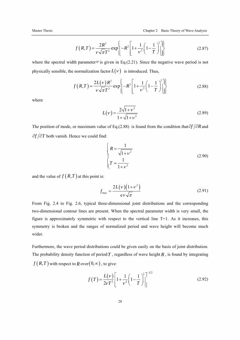
where the spectral width parameterν is given in Eq.(2.21). Since the negative wave period is not
physically sensible, the normalization factor ( )L ν is introduced. Thus,
( ) ( ) 222
22
2 1 1, exp 1 1L R
f R T RTT
ννν π
⎧ ⎫⎡ ⎤⎪ ⎪⎛ ⎞= − + −⎢ ⎥⎨ ⎬⎜ ⎟⎝ ⎠⎢ ⎥⎪ ⎪⎣ ⎦⎩ ⎭
(2.88)
where
( )2
2
2 11 1
L ννν
+=
+ + (2.89)
The position of mode, or maximum value of Eq.(2.88) is found from the condition that f R∂ ∂ and
f T∂ ∂ both vanish. Hence we could find:
2
2
111
1
R
T
ν
ν
⎧ =⎪⎪ +⎨⎪ =⎪ +⎩
(2.90)
and the value of ( ),f R T at this point is:
( )( )2
max
2 1
e
Lf
ν ν
ν π
+= (2.91)
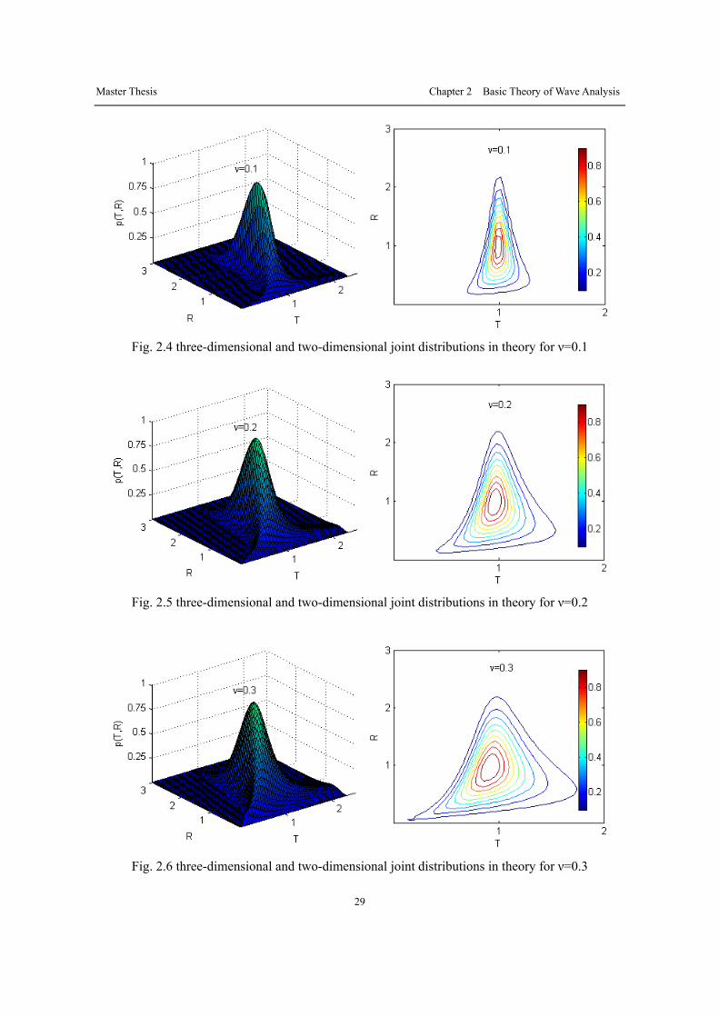
From Fig. 2.4 to Fig. 2.6, typical three-dimensional joint distributions and the corresponding
two-dimensional contour lines are present. When the spectral parameter width is very small, the
figure is approximately symmetric with respect to the vertical line T=1. As it increases, this
symmetry is broken and the ranges of normalized period and wave height will become much
wider.
Furthermore, the wave period distributions could be given easily on the basis of joint distribution.
The probability density function of periodT , regardless of wave height R , is found by integrating
( ),f R T with respect to R over ( )0,∞ , to give:
( ) ( )3 22
2 2
1 11 12L
f TT Tν
ν ν
−⎡ ⎤⎛ ⎞= + −⎢ ⎥⎜ ⎟
⎝ ⎠⎢ ⎥⎣ ⎦ (2.92)
Master Thesis Chapter 2 Basic Theory of Wave Analysis
29
Fig. 2.4 three-dimensional and two-dimensional joint distributions in theory for ν=0.1
Fig. 2.5 three-dimensional and two-dimensional joint distributions in theory for ν=0.2
Fig. 2.6 three-dimensional and two-dimensional joint distributions in theory for ν=0.3

Master T
Ch
3.1
Wave
one en
basin.
offshor
As sho
spaced
the wa
simulta
is 30m
series
Thesis
hapter 3
Facility a
tanks are us
nd. In the exp
The beach a
re basin in th
own in Fig.
d along the w
ave maker an
aneously 10
m now and th
is nearly hal
and Data
sually charac
periment, the
at the oppos
he Technical
F
3.2, the wat
wave basin at
nd the same
meters away
he same exp
lf an hour wi
Exper
cterized as lo
e double-flap
ite side serv
University o
Fig. 3.1 Dim
Fig. 3.2 P
ter surface e
t 20m interv
experiment
y from the w
periment is r
ith sampling
30
riment R
ong, narrow
p wave make
ves to absorb
of Berlin is 1
mensions of o
osition of wa
elevations ha
al. In the firs
is done two
wave make. T
repeated as b
g frequency 1
Chapter 3
Results of
enclosures w
er is installed
b the inciden
152m×30m×5
offshore basin
ave gauges
ave been me
st test, the fi
times. Then
That is, the n
before. The
100Hz. The
Experiment Re
f Wave A
with some k
d at one of th
nt wave ener
5m as show
n
easured by 6
rst gauge is
n the 6 wave
earest gauge
duration of
scale of this
esults of Wave A
Analysis
kind wave-m
he short walls
rgy. The size
in Fig. 3.1.
6 gauges uni
20m far awa
e gauges are
e to the wave
each recorde
experiment
Analysis
s
maker at
s of the
e of the
iformly
ay from
moved
e maker
ed time
is 1:50
Master Thesis Chapter 3 Experiment Results of Wave Analysis
31
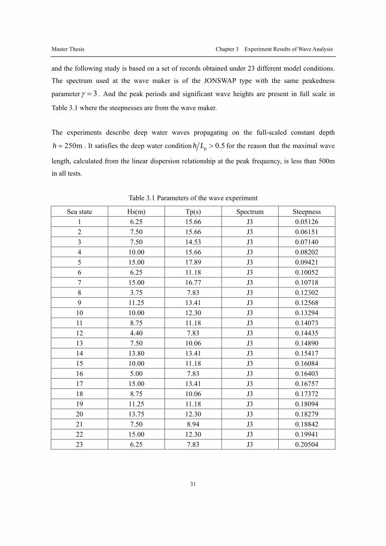
and the following study is based on a set of records obtained under 23 different model conditions.
The spectrum used at the wave maker is of the JONSWAP type with the same peakedness
parameter 3γ = . And the peak periods and significant wave heights are present in full scale in
Table 3.1 where the steepnesses are from the wave maker.
The experiments describe deep water waves propagating on the full-scaled constant depth
250mh = . It satisfies the deep water condition p 0.5h L > for the reason that the maximal wave
length, calculated from the linear dispersion relationship at the peak frequency, is less than 500m
in all tests.
Table 3.1 Parameters of the wave experiment
Sea state Hs(m) Tp(s) Spectrum Steepness 1 6.25 15.66 J3 0.05126 2 7.50 15.66 J3 0.06151 3 7.50 14.53 J3 0.07140 4 10.00 15.66 J3 0.08202 5 15.00 17.89 J3 0.09421 6 6.25 11.18 J3 0.10052 7 15.00 16.77 J3 0.10718 8 3.75 7.83 J3 0.12302 9 11.25 13.41 J3 0.12568
10 10.00 12.30 J3 0.13294 11 8.75 11.18 J3 0.14073 12 4.40 7.83 J3 0.14435 13 7.50 10.06 J3 0.14890 14 13.80 13.41 J3 0.15417 15 10.00 11.18 J3 0.16084 16 5.00 7.83 J3 0.16403 17 15.00 13.41 J3 0.16757 18 8.75 10.06 J3 0.17372 19 11.25 11.18 J3 0.18094 20 13.75 12.30 J3 0.18279 21 7.50 8.94 J3 0.18842 22 15.00 12.30 J3 0.19941 23 6.25 7.83 J3 0.20504

Master Thesis Chapter 3 Experiment Results of Wave Analysis
32
Fig. 3.3 Time series cut from gauge 1
Fig. 3.4 Time series cut from gauge 3
Fig. 3.5 Time series cut from gauge 5

Master Thesis Chapter 3 Experiment Results of Wave Analysis
33
Considering that only 6 wave records are made at a time for each sea state, it is better to present
the results with six gauges each time by the mean value in the same position. The respective mean
results of the six gauges in the first position are denoted as Part A in the following analysis and the
corresponding mean results in the second position are denoted as Part B. The initial steepness
mentioned is the steepness measured at the first gauge in Part A and Part B respectively.
In order to make sure that the initial noise is cut off and that the waves analyzed from 6 gauges are
the same, it is necessary to cut off the wave record at the right position by utilizing the wave group
velocity as done in Fig. 3.3~Fig. 3.5.

Master Thesis Chapter 3 Statistical Analysis of Surface Wave
34
3.2 Spectral Analysis
3.2.1 Spectral Comparison
With the help of Blackman-Tukey method and Cooley-Tukey method mentioned in chapter 2, the
wave record in each gauge generates two wave spectra which are compared with the standard
JONSWAP spectrum described in Eq.(2.28) where significant wave height and peak period are the
expected values from the former two methods. For the purpose of simplicity, only the figures of
Gauge1, Gauge4 and Gauge6 are presented below in three typical sea states which are
characterized by different initial steepness. These three gauges could reflect the spatial variation of
the wave spectra very well, because Gauge1 is the nearest point to the wave maker which shows
what happens at the beginning; Gauge4 is in the middle of the wave basin which shows what
appears at the intermediate position; Gauge6 is the longest distance from the wave maker which
shows what could be present at the end of the wave basin.
As it is shown in the Fig. 3.6, ‘G1’,’G4’ and ’G6’ stands for three gauges respectively. ‘BT’,’CT’
and ‘Sta’ successively denote spectra obtained with Blackman-Tukey Method, Cooley-Tukey
Method and the standard one proposed by Goda (1988). According to the experiment, it is noted
that the two methods do not give two much difference except for the density of peak frequency.
When the initial steepness is very small, the computed wave spectra are exactly the same as the
standard one as shown in Fig. 3.6.
Fig. 3.6 Wave spectra with initial steepness s0=0.0514
When the initial steepness increases, the computed spectra will deviate from the standard one.
With reference to Fig. 3.7, in the sea state with intermediate initial steepness, the computed spectra
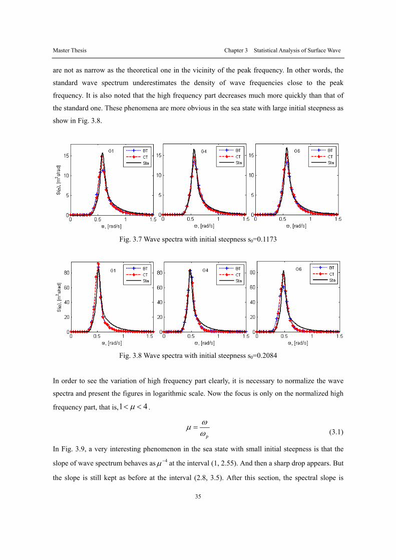
Master Thesis Chapter 3 Statistical Analysis of Surface Wave
35
are not as narrow as the theoretical one in the vicinity of the peak frequency. In other words, the
standard wave spectrum underestimates the density of wave frequencies close to the peak
frequency. It is also noted that the high frequency part decreases much more quickly than that of
the standard one. These phenomena are more obvious in the sea state with large initial steepness as
show in Fig. 3.8.
Fig. 3.7 Wave spectra with initial steepness s0=0.1173
Fig. 3.8 Wave spectra with initial steepness s0=0.2084
In order to see the variation of high frequency part clearly, it is necessary to normalize the wave
spectra and present the figures in logarithmic scale. Now the focus is only on the normalized high
frequency part, that is,1 4μ< < .
p
ωμω
= (3.1)
In Fig. 3.9, a very interesting phenomenon in the sea state with small initial steepness is that the
slope of wave spectrum behaves as 4μ− at the interval (1, 2.55). And then a sharp drop appears. But
the slope is still kept as before at the interval (2.8, 3.5). After this section, the spectral slope is

Master Thesis Chapter 3 Statistical Analysis of Surface Wave
36
steepened to about 6μ− due to the viscous dissipation (Fedele et al., 2010). It plays a major role
when the initial wave steepness is not large enough in the wave basin. In other word, when the
initial steepness is very small, it is the viscous effect that dissipates the high frequency wave
energy.
When the initial steepness increases to 0.0879 as present in Fig. 3.10, wave breaking begins to
dissipate wave energy with the viscous effect. Moreover, since the part of 5μ− increases along the
wave basin, it means more and more energy is dissipated in the propagation.
Fig. 3.9 Normalized wave spectra with initial steepness s0=0.0514
Fig. 3.10 Normalized wave spectra with initial steepness s0=0.0879
As the initial steepness continues to increase, the turning point of spectral slopes moves quickly to
1μ = . This is confirmed explicitly if comparing Fig. 3.11 and Fig. 3.12 together. In Fig. 3.12,
since the initial steepness is really high, the spectral slopes tend to behave as 5μ− above the peak
frequency. In other words, the wave breaking is really severe and dissipates the most energy in the
high frequency part.

Master Thesis Chapter 3 Statistical Analysis of Surface Wave
37
Fig. 3.11 Normalized wave spectra with initial steepness s0=0.1152
Fig. 3.12 Normalized wave spectra with initial steepness s0=0.2084
3.2.2 Significant Wave Height
The change of the significant wave heights (Hs) along the wave basin could be catalogued into
three groups and attributed to two reasons. The major factor that affects the evolution trend is the
initial wave steepness. Normally, if the initial steepness is smaller than one specific value, the
significant wave height will increase along the wave basin while if it is larger than another specific
value, the significant wave height will decrease. Between these two values, the general trend will
maintain level. The critical values of initial steepness found in the experiment are listed in Table
3.2. Initial steepness used below for classification is the mean value of the first steepness in part A
and part B.
Table 3.2 Critical value of initial steepness for the evolution trend of Hs
Group Initial Steepness Trend 1 0.0514 0.1086 Ascended 2 0.1148 0.1680 Level 3 0.1702 0.2100 Descended
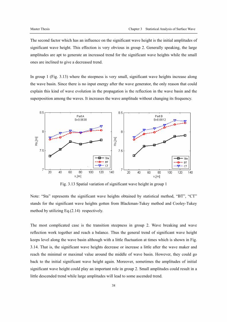
Master Thesis Chapter 3 Statistical Analysis of Surface Wave
38
The second factor which has an influence on the significant wave height is the initial amplitudes of
significant wave height. This effection is very obvious in group 2. Generally speaking, the large
amplitudes are apt to generate an increased trend for the significant wave heights while the small
ones are inclined to give a decreased trend.
In group 1 (Fig. 3.13) where the steepness is very small, significant wave heights increase along
the wave basin. Since there is no input energy after the wave generator, the only reason that could
explain this kind of wave evolution in the propagation is the reflection in the wave basin and the
superposition among the waves. It increases the wave amplitude without changing its frequency.
Fig. 3.13 Spatial variation of significant wave height in group 1
Note: “Sta” represents the significant wave heights obtained by statistical method, “BT”, “CT”
stands for the significant wave heights gotten from Blackman-Tukey method and Cooley-Tukey
method by utilizing Eq.(2.14) respectively.
The most complicated case is the transition steepness in group 2. Wave breaking and wave
reflection work together and reach a balance. Thus the general trend of significant wave height
keeps level along the wave basin although with a little fluctuation at times which is shown in Fig.
3.14. That is, the significant wave heights decrease or increase a little after the wave maker and
reach the minimal or maximal value around the middle of wave basin. However, they could go
back to the initial significant wave height again. Moreover, sometimes the amplitudes of initial
significant wave height could play an important role in group 2. Small amplitudes could result in a
little descended trend while large amplitudes will lead to some ascended trend.
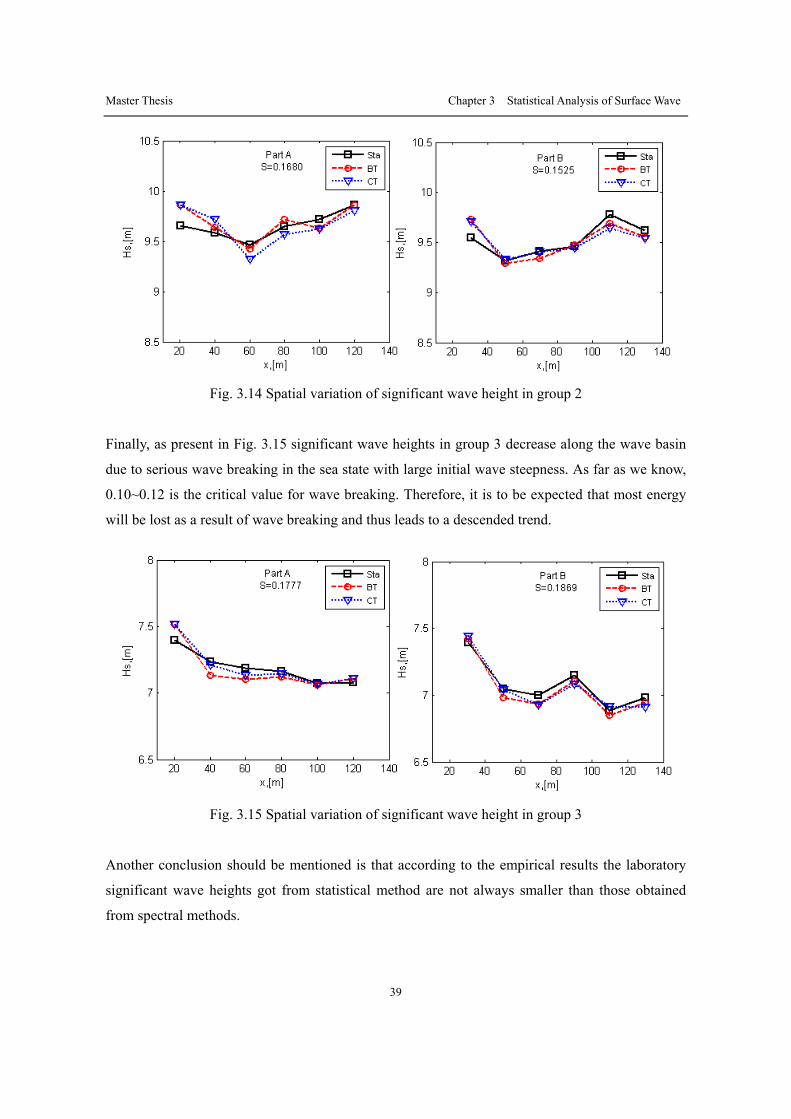
Master Thesis Chapter 3 Statistical Analysis of Surface Wave
39
Fig. 3.14 Spatial variation of significant wave height in group 2
Finally, as present in Fig. 3.15 significant wave heights in group 3 decrease along the wave basin
due to serious wave breaking in the sea state with large initial wave steepness. As far as we know,
0.10~0.12 is the critical value for wave breaking. Therefore, it is to be expected that most energy
will be lost as a result of wave breaking and thus leads to a descended trend.
Fig. 3.15 Spatial variation of significant wave height in group 3
Another conclusion should be mentioned is that according to the empirical results the laboratory
significant wave heights got from statistical method are not always smaller than those obtained
from spectral methods.
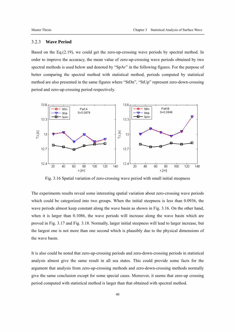
Master Thesis Chapter 3 Statistical Analysis of Surface Wave
40
3.2.3 Wave Period
Based on the Eq.(2.19), we could get the zero-up-crossing wave periods by spectral method. In
order to improve the accuracy, the mean value of zero-up-crossing wave periods obtained by two
spectral methods is used below and denoted by “SpAv” in the following figures. For the purpose of
better comparing the spectral method with statistical method, periods computed by statistical
method are also presented in the same figures where “StDn”, “StUp” represent zero-down-crossing
period and zero-up-crossing period respectively.
Fig. 3.16 Spatial variation of zero-crossing wave period with small initial steepness
The experiments results reveal some interesting spatial variation about zero-crossing wave periods
which could be categorized into two groups. When the initial steepness is less than 0.0936, the
wave periods almost keep constant along the wave basin as shown in Fig. 3.16. On the other hand,
when it is larger than 0.1086, the wave periods will increase along the wave basin which are
proved in Fig. 3.17 and Fig. 3.18. Normally, larger initial steepness will lead to larger increase, but
the largest one is not more than one second which is plausibly due to the physical dimensions of
the wave basin.
It is also could be noted that zero-up-crossing periods and zero-down-crossing periods in statistical
analysis almost give the same result in all sea states. This could provide some facts for the
argument that analysis from zero-up-crossing methods and zero-down-crossing methods normally
give the same conclusion except for some special cases. Moreover, it seems that zero-up crossing
period computed with statistical method is larger than that obtained with spectral method.

Master Thesis Chapter 3 Statistical Analysis of Surface Wave
41
Fig. 3.17 Spatial variation of zero-crossing wave period with intermediate initial steepness
Fig. 3.18 Spatial variation of zero-crossing wave period with large initial steepness
Another very useful wave period in spectral analysis is the mean spectral period as expressed in
Eq.(2.17). Considering that the spatial variation of zero crossing wave periods is almost linear, it is
feasible to measure the change of mean spectral periods during the propagation along the tank by
the ratio between the value measured in the longest distance to the value measured closest to the
wave maker, proposed by Cherneva and Guedes Soares (2011). This ratio is denoted by index (r)
to differ from the relevant parameters.
Since the reciprocal value of the mean spectral period which is known as the carrier frequency has
more physical meaning, the relative carrier frequency as a function of initial steepness for all sea

Master Thesis Chapter 3 Statistical Analysis of Surface Wave
42
states is preferred and plotted in Fig. 3.19. It is certain that the relative frequency is equal or small
than 1. The series with higher nonlinearity characterized by large initial steepness are modulated
more due to the reduction of the spectrum tail in its high frequency part as found previously in
section 3.2.1.
Fig. 3.19 Relationship between relative carrier frequency and initial steepness
3.2.4 Zero Spectral Moment and Steepness
Since we have analyzed the spatial variation of significant wave heights, it is not difficult to
predict the propagation law of the zero spectral moments along the wave basin for the reason that
they have a direct relationship as listed in Eq.(2.14). All the conclusions made in section 3.2.2 still
hold for the zero spectral moment. In the following three figures, “m0” denotes the mean zero
spectral moment obtained by “BT” and “CT” spectral methods. And “steep” stands for the wave
steepness of each gauge. The two independent variables have the same dependent variable which
is the distance from the wave maker. But their values are presented in different vertical axes. The
left one is for zero spectral moment while the right one is for wave steepness.
It is pronounced that the change of wave steepness is almost in direct proportion to the change of
zero spectral moment and also depends on the initial steepness. It is obviously correct in that when
the wave energy is large, that is, large zero spectral moment, it definitely will generate large wave
height and thus results in large steepness at that position. Therefore, the spatial variation of
steepness will be the same as that of significant wave height.

Master Thesis Chapter 3 Statistical Analysis of Surface Wave
43
Fig. 3.20 Spatial variation of m0 and steepness with small initial steepness
Fig. 3.21 Spatial variation of m0 and steepness with intermediate initial steepness
Fig. 3.22 Spatial variation of m0 and steepness with large initial steepness

Master Thesis Chapter 3 Statistical Analysis of Surface Wave
44
For the sake of observing the relationship between the change of wave energy and the initial
steepness clearly, the ratio of the sixth zero spectral moment in the wave basin to the first one
could be used again as a parameter as mentioned by Cherneva and Guedes Soares (2011). One
thing should be kept in mind is that only for large and small initial steepness, Fig. 3.23 could
reflect the change of wave energy well while for the intermediate initial steepness, this method
does not always work due to the irregular variation as shown in Fig. 3.21.
As shown in the experiment, the relative zero spectral moment is larger than 1.0 in the case of
small initial steepness. In other words, the waver energy is increased nearly 10% plausibly because
of the reflection in the wave basin. When initial steepness is larger than 0.1, the increase speed is
not as fast as before which means that the speed of energy dissipation is much faster. As initial
steepness continues to increase, wave breaking plays a more and more important role in the
dissipation of energy and thus leads to a further decrease in relative zero spectral moment. The
largest decrease is nearly 15% and the second critical change point of initial steepness in the
experiment is near to 0.15 where the total wave energy begins to decrease. It is demonstrated in the
value of relative zero spectral moment less than 1.0.
Fig. 3.23 Relationship between relative zero spectral moment and initial steepness
3.2.5 Spectral Width Parameter
One of the most important parameters in spectral analysis is the spectral width parameter described
in Eq.(2.21) and Eq.(2.23). According to the experiment, a very interesting phenomenon is that
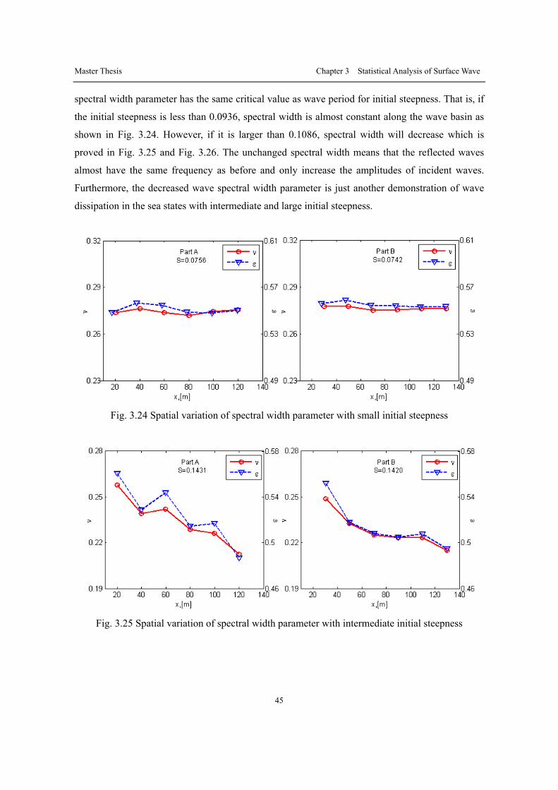
Master Thesis Chapter 3 Statistical Analysis of Surface Wave
45
spectral width parameter has the same critical value as wave period for initial steepness. That is, if
the initial steepness is less than 0.0936, spectral width is almost constant along the wave basin as
shown in Fig. 3.24. However, if it is larger than 0.1086, spectral width will decrease which is
proved in Fig. 3.25 and Fig. 3.26. The unchanged spectral width means that the reflected waves
almost have the same frequency as before and only increase the amplitudes of incident waves.
Furthermore, the decreased wave spectral width parameter is just another demonstration of wave
dissipation in the sea states with intermediate and large initial steepness.
Fig. 3.24 Spatial variation of spectral width parameter with small initial steepness
Fig. 3.25 Spatial variation of spectral width parameter with intermediate initial steepness
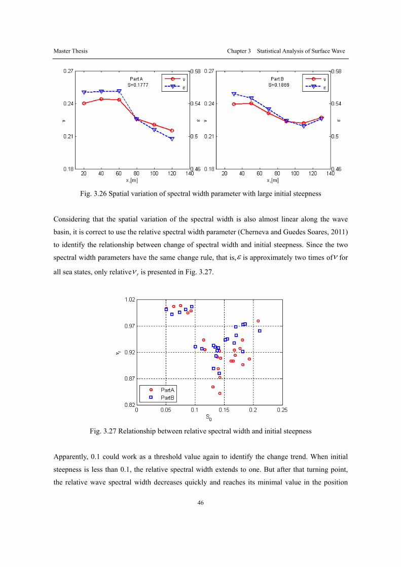
Master Thesis Chapter 3 Statistical Analysis of Surface Wave
46
Fig. 3.26 Spatial variation of spectral width parameter with large initial steepness
Considering that the spatial variation of the spectral width is also almost linear along the wave
basin, it is correct to use the relative spectral width parameter (Cherneva and Guedes Soares, 2011)
to identify the relationship between change of spectral width and initial steepness. Since the two
spectral width parameters have the same change rule, that is,ε is approximately two times ofν for
all sea states, only relative rν is presented in Fig. 3.27.
Fig. 3.27 Relationship between relative spectral width and initial steepness
Apparently, 0.1 could work as a threshold value again to identify the change trend. When initial
steepness is less than 0.1, the relative spectral width extends to one. But after that turning point,
the relative wave spectral width decreases quickly and reaches its minimal value in the position

Master Thesis Chapter 3 Statistical Analysis of Surface Wave
47
where the initial wave steepness is near 0.15. And then, the relative wave spectral width parameter
increases but still smaller than 1.0. Whatever, it could be noted that the averaged decrease is nearly
8% in most cases. The last thing that needs to be emphasized is that all the wave spectral widthsν
are in the range from 0.2 to 0.3 in the experiment which could be considered as narrow band
spectra. It is very strange that the maximal decrease is present in the intermediate sea state rather
than the most serious one.

Master Thesis Chapter 3 Statistical Analysis of Surface Wave
48
3.3 Statistical Analysis
3.3.1 Skewness and Kurtosis
Skewness and kurtosis are two important parameters in statistics analysis. As mentioned above,
only when the kurtosis and skewness are both closed to zero, wave surface displacements could be
considered as Gaussian as presented in (A) of Fig. 3.28. More often than not, the most common
distribution appeared in the experiment is presented in (B) of Fig. 3.28 where the peak value is
located smaller than the mean value zero because of the positive skewness and it is sharper than (A)
due to the large positive kurtosis.
Fig. 3.28 Distribution of normalized surface displacement in the experiment
In the laboratory experiment, only in the case of very small initial steepness, the coefficient of
kurtosis is negative as presented in the first picture of Fig. 3.29 and Fig. 3.30. When the initial
steepness is intermediate or large, it is positive and increases to a maximal value at about 60m
from the wave maker. It is constant in the later propagation. The same spatial variation was
presented by Petrova et al. (2008). At the place near to wave maker, the third order nonlinearity
effect is not very strong because its value is very small. What is more, the largest kurtosis appears
in the sea state with intermediate initial steepness rather than the largest one. That is also what
happens to the decrease of spectral width parameter discussed in section 3.2.5. The coefficient of
skewness is almost positive everywhere and its spatial variation is very small along the wave basin.
It means that the second order nonlinear effect is constant along the wave basin. Moreover, larger
coefficient of skewness is related with larger initial steepness, that is, the severer sea state.
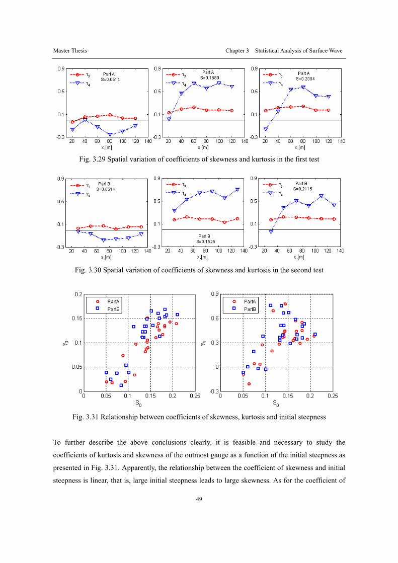
Master Thesis Chapter 3 Statistical Analysis of Surface Wave
49
Fig. 3.29 Spatial variation of coefficients of skewness and kurtosis in the first test
Fig. 3.30 Spatial variation of coefficients of skewness and kurtosis in the second test
Fig. 3.31 Relationship between coefficients of skewness, kurtosis and initial steepness
To further describe the above conclusions clearly, it is feasible and necessary to study the
coefficients of kurtosis and skewness of the outmost gauge as a function of the initial steepness as
presented in Fig. 3.31. Apparently, the relationship between the coefficient of skewness and initial
steepness is linear, that is, large initial steepness leads to large skewness. As for the coefficient of
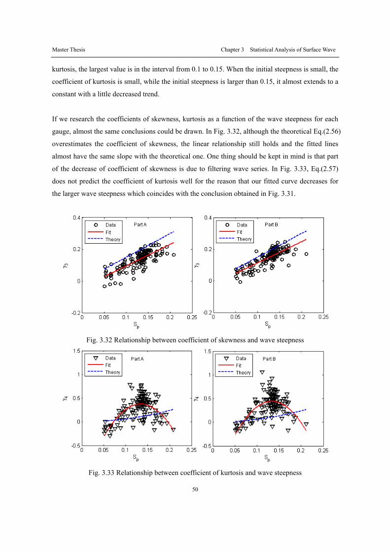
Master Thesis Chapter 3 Statistical Analysis of Surface Wave
50
kurtosis, the largest value is in the interval from 0.1 to 0.15. When the initial steepness is small, the
coefficient of kurtosis is small, while the initial steepness is larger than 0.15, it almost extends to a
constant with a little decreased trend.
If we research the coefficients of skewness, kurtosis as a function of the wave steepness for each
gauge, almost the same conclusions could be drawn. In Fig. 3.32, although the theoretical Eq.(2.56)
overestimates the coefficient of skewness, the linear relationship still holds and the fitted lines
almost have the same slope with the theoretical one. One thing should be kept in mind is that part
of the decrease of coefficient of skewness is due to filtering wave series. In Fig. 3.33, Eq.(2.57)
does not predict the coefficient of kurtosis well for the reason that our fitted curve decreases for
the larger wave steepness which coincides with the conclusion obtained in Fig. 3.31.
Fig. 3.32 Relationship between coefficient of skewness and wave steepness
Fig. 3.33 Relationship between coefficient of kurtosis and wave steepness
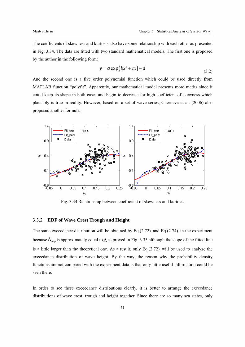
Master Thesis Chapter 3 Statistical Analysis of Surface Wave
51
The coefficients of skewness and kurtosis also have some relationship with each other as presented
in Fig. 3.34. The data are fitted with two standard mathematical models. The first one is proposed
by the author in the following form:
( )3exp bx cxy a d+= + (3.2)
And the second one is a five order polynomial function which could be used directly from
MATLAB function “polyfit”. Apparently, our mathematical model presents more merits since it
could keep its shape in both cases and begin to decrease for high coefficient of skewness which
plausibly is true in reality. However, based on a set of wave series, Cherneva et al. (2006) also
proposed another formula.
Fig. 3.34 Relationship between coefficient of skewness and kurtosis
3.3.2 EDF of Wave Crest Trough and Height
The same exceedance distribution will be obtained by Eq.(2.72) and Eq.(2.74) in the experiment
because appΛ is approximately equal toΛ as proved in Fig. 3.35 although the slope of the fitted line
is a little larger than the theoretical one. As a result, only Eq.(2.72) will be used to analyze the
exceedance distribution of wave height. By the way, the reason why the probability density
functions are not compared with the experiment data is that only little useful information could be
seen there.
In order to see these exceedance distributions clearly, it is better to arrange the exceedance
distributions of wave crest, trough and height together. Since there are so many sea states, only
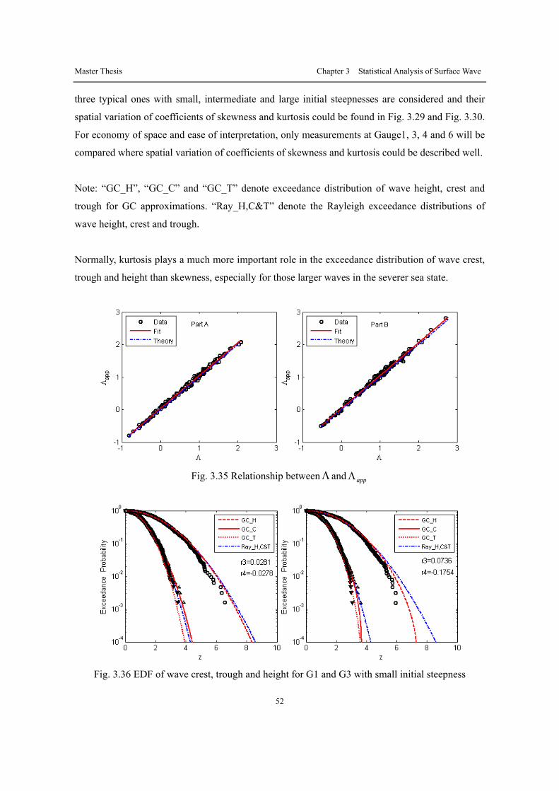
Master Thesis Chapter 3 Statistical Analysis of Surface Wave
52
three typical ones with small, intermediate and large initial steepnesses are considered and their
spatial variation of coefficients of skewness and kurtosis could be found in Fig. 3.29 and Fig. 3.30.
For economy of space and ease of interpretation, only measurements at Gauge1, 3, 4 and 6 will be
compared where spatial variation of coefficients of skewness and kurtosis could be described well.
Note: “GC_H”, “GC_C” and “GC_T” denote exceedance distribution of wave height, crest and
trough for GC approximations. “Ray_H,C&T” denote the Rayleigh exceedance distributions of
wave height, crest and trough.
Normally, kurtosis plays a much more important role in the exceedance distribution of wave crest,
trough and height than skewness, especially for those larger waves in the severer sea state.
Fig. 3.35 Relationship betweenΛ and appΛ
Fig. 3.36 EDF of wave crest, trough and height for G1 and G3 with small initial steepness

Master Thesis Chapter 3 Statistical Analysis of Surface Wave
53
Fig. 3.37 EDF of wave crest, trough and height for G4 and G6 with small initial steepness
In Fig. 3.36 and Fig. 3.37, when the initial steepness is very small, skewness and kurtosis will not
be very large anywhere in the wave basin. Thus leads to that the GC distribution is almost
consistent with the Rayleigh distribution except for a little difference in the middle of the wave
basin where both of them overestimate the larger wave heights. The theoretical modals of wave
crest and trough agree with the experiment data reasonably well and they almost overlap with each
other satisfying the linear wave theory.
Fig. 3.38 EDF of wave crest, trough and height for G1 and G3 with intermediate initial steepness
In Fig. 3.38 and Fig. 3.39, the coefficients of skewness and kurtosis are both positive and very
large in the sea state with intermediate initial steepness. As a result, GC approximations for wave
crest and height largely deviate from the Rayleigh distribution. What is more, GC approximation
could predict the experiment data better in most cases comparing with the Rayleigh distribution.

Master Thesis Chapter 3 Statistical Analysis of Surface Wave
54
The overestimation is due to wave breaking in the offshore basin and filtering wave at the
beginning.
Fig. 3.39 EDF of wave crest, trough and height for G4 and G6 with intermediate initial steepness
Fig. 3.40 EDF of wave crest, trough and height for G1 and G3 with large initial steepness
Fig. 3.41 EDF of wave crest, trough and height for G4 and G6 with large initial steepness

Master Thesis Chapter 3 Statistical Analysis of Surface Wave
55
For the case of large initial steepness as shown in Fig. 3.40 and Fig. 3.41, almost the same rules
could be obtained as the case of intermediate initial steepness except for the very large wave
height and crest. Considering that the more serious sea state generates more wave breaking, it is no
wonder that exceedance probability will drop in larger wave part in Gauge3 and Gauge4 because
of the very large kurtosis. Although GC approximation overestimates the wave crest, it is still
much better than Rayleigh distribution. Cherneva, Tayfun and Guedes Soares (2009) also pointed
out that GC approximation could not fit the empirical data well sometimes. Last, although kurtosis
is negative at the gauge near to the wave maker, GC approximation could predict the exceedance
distribution reasonably well.
Finally, based on what we have discussed above, it is strongly supported that GC approximations
could predict wave crest and height much better than Rayleigh distribution in most cases.
3.3.3 Wave Period
In section 3.2.3, the spatial variation of specified wave periods has been researched with spectral
method for different sea states. Now we will consider the distributions of wave periods in a
statistical view. The theoretical distribution in Eq.(2.92) is only related to the wave spectral width,
and section 3.2.5 has proved that the variation of wave spectral width is not large enough to
apparently affect the theoretical distribution.
From Fig. 3.42 to Fig. 3.44, periods from three represented sea states are chosen where“ν ”and“S ”
stand for the spectral width parameter and the wave steepness for each gauge respectively.
Obviously, the theoretical wave period distribution changes slowly because the spectral width
parameter does not decrease quickly as the sea state changes. However, the distribution of
observed wave period changes rapidly and the shape becomes sharper and narrower as the wave
steepness increases. Therefore, the wave period distribution should be related not only with the
wave spectral width parameter but also with the initial wave steepness. It seems that the wave
periods are asymptotically uniformly distributed around the carrier wave period when the sea state
is mild as described in Fig. 3.42. As the sea state becomes severer, the periods will concentrate on
the peak wave period which is a little larger than the carrier wave period as presented in Fig. 3.43
and Fig. 3.44. Moreover, the wave period will increase along the wave basin as we discussed in
spectral analysis.
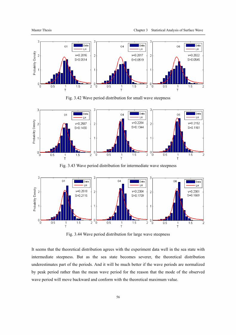
Master Thesis Chapter 3 Statistical Analysis of Surface Wave
56
Fig. 3.42 Wave period distribution for small wave steepness
Fig. 3.43 Wave period distribution for intermediate wave steepness
Fig. 3.44 Wave period distribution for large wave steepness
It seems that the theoretical distribution agrees with the experiment data well in the sea state with
intermediate steepness. But as the sea state becomes severer, the theoretical distribution
underestimates part of the periods. And it will be much better if the wave periods are normalized
by peak period rather than the mean wave period for the reason that the mode of the observed
wave period will move backward and conform with the theoretical maximum value.
Master Thesis Chapter 3 Statistical Analysis of Surface Wave
57
3.3.4 Joint Distribution
From Fig. 3.45 to Fig. 3.50, the theoretical joint distribution and the experiment data are compared
together. In the same manner as wave period distribution, only figures of three typical sea states
are presented below. The symbols “Pomax” and “Ptmax” successively denote observed maximal
probability and theoretical maximal probability. The other symbols are still the same as before.
The black asterisk represents the location of the observed maximal probability which may be not
only one sometimes. In order to describe the comparison clearly, the probabilities are normalized
by the maximal probability respectively when plotting the theoretical contour lines and drawing
the experiment data with different colors.
Apparently, the mean spectral width parameter does not decrease too much and thus the theoretical
joint distribution almost keeps the same shape for all sea states for the reason that spectral width
parameter is the only variable in Eq.(2.88). However, the observed distribution changes greatly as
the wave steepness increases.
For the mild sea state, this theoretical joint distribution does not predict the experiment result well
although the maximal value seems good. The observed shape is more or less like a triangle and it
is obvious that the large wave period and large wave height are not enough to fit the theoretical
distribution. Sharpe (1990) once obtained the same result without explaining the reasons. If we
review the deducing procedure, Longuet-Higgins once assumed the wave frequencies mainly
concentrated on the carrier wave frequency and thus leaded to the bad prediction in the sea state
with small initial steepness considering that Fig. 3.42 presents an approximately flat distribution
for the wave periods rather than a sharp one.
As the sea state becomes serous, the theoretical joint distribution agrees with the observed data
reasonably well. Therefore, the theoretical joint distribution should be not only related to the wave
spectral width parameter but also connected with the initial wave steepness. The theoretical joint
distribution is also based on the linear superposition which may be not suitable in the severe sea
state due to the strong nonlinearity and thus maybe explain the deviation from the observed results.

Master Thesis Chapter 3 Statistical Analysis of Surface Wave
58
Fig. 3.45 Joint distribution with small initial wave steepness 1
Fig. 3.46 Joint distribution with small wave steepness 2
Fig. 3.47 Joint distribution with intermediate initial wave steepness 1

Master Thesis Chapter 3 Statistical Analysis of Surface Wave
59
Fig. 3.48 Joint distribution with intermediate initial wave steepness 2
Fig. 3.49 Joint distribution with large initial wave steepness 1
Fig. 3.50 Joint distribution for large initial wave steepness 2

Master Thesis Chapter 3 Statistical Analysis of Surface Wave
60
If we check the location of the observed maximal probability from Fig. 3.47 to Fig. 3.50, it is very
interesting that the observed positions stay in the bottom right corner of the theoretical location in
most cases. It means that the parameter for normalizing wave periods is too small while the
parameter for normalizing wave heights is too large. Therefore, the peak wave periods may be a
better choice as we have proposed in section 3.3.3. Maybe another smaller parameter should be
chosen to replace the mean-square value of wave height. But the shape of the theoretical
distribution will also be changed at the same time. Apparently, this topic could be further
continued but is out of the scope of this thesis.
3.3.5 Maximal Wave Height
The prediction of location of the maximal wave height in the wave basin will be really useful if we
do some research on the freak waves. But according to the experiment, it is found that the spatial
variation of maximal wave height is rather complicated and irregular. Even for the same sea state,
different experiments normally present different variations. Only in several sea states such as
presented in Fig. 3.51, a general trend could be obtained from the two tests. Therefore, statistical
distribution will be much better for describing the spatial variation of maximal wave height.
Fig. 3.51 Spatial variation of maximal wave height
In Fig. 3.52, the relationship between the maximal wave height and the corresponding period is
researched. “ZeroUp” and “ZeroDn” represent the experiment data obtained from the analysis of
zero-up-crossing wave points and zero-down-crossing points respectively. Apparently, the fitted
lines are nearly overlapped with each other. That is, analysis of zero-up-crossing points or

Master Thesis Chapter 3 Statistical Analysis of Surface Wave
61
zero-down-crossing points does not have too much difference. Moreover, as maximal wave height
increases, the related wave period will increase. What calls for special attentions is that there
seems to be two functions for the maximal wave height and period. One is linear and the other
needs to be further researched to check if it is true.
Fig. 3.52 Relationship between maximal wave height and the corresponding wave period
Fig. 3.53 Relationship between initial steepness and maximal wave steepness
The last very interesting relationship for the maximal wave height in this thesis is shown in Fig.
3.53 where “Data1” and “Data2” are only different in “L” used for the computation of vertical
coordinates. L is obtained from wave period T by the linear dispersion relationship. For “Data1”, T
is the period related with the maximal wave height. And for “Data2”, T represents the peak wave
period. “S0” stands for the initial wave steepness and the black dash line represents the Stockes
Master Thesis Chapter 3 Statistical Analysis of Surface Wave
62
limit. It is obvious that the maximal wave steepness will increase as the initial steepness increases
and reach a maximal value when the initial steepness is around 0.17. After that, it will begin to fall
down due to the serious wave breaking. This change is consistent with the result obtained by
Cherneva and Guedes Soares (2011). One interesting phenomenon is that the red solid line almost
presents the same change rule as the blue dot dash line. In other words, the period corresponding
to maximal wave height is directly proportional to the peak wave period. The blue dot dash line
has more realistic meaning in application because if it could be obtained from a wave basin, it will
be convenient for the researcher to design the wave experiment to obtain the desired maximal
wave height.
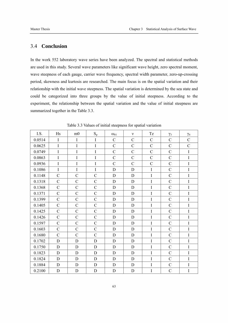
Master Thesis Chapter 3 Statistical Analysis of Surface Wave
63
3.4 Conclusion
In the work 552 laboratory wave series have been analyzed. The spectral and statistical methods
are used in this study. Several wave parameters like significant wave height, zero spectral moment,
wave steepness of each gauge, carrier wave frequency, spectral width parameter, zero-up-crossing
period, skewness and kurtosis are researched. The main focus is on the spatial variation and their
relationship with the initial wave steepness. The spatial variation is determined by the sea state and
could be categorized into three groups by the value of initial steepness. According to the
experiment, the relationship between the spatial variation and the value of initial steepness are
summarized together in the Table 3.3.
Table 3.3 Values of initial steepness for spatial variation
I.S. Hs m0 Sp ω01 ν Tz γ3 γ4 0.0514 I I I C C C C C 0.0625 I I I C C C C C 0.0749 I I I C C C C I 0.0863 I I I C C C C I 0.0936 I I I C C C C I 0.1086 I I I D D I C I 0.1148 C C C D D I C I 0.1318 C C C D D I C I 0.1368 C C C D D I C I 0.1371 C C C D D I C I 0.1399 C C C D D I C I 0.1405 C C C D D I C I 0.1425 C C C D D I C I 0.1426 C C C D D I C I 0.1597 C C C D D I C I 0.1603 C C C D D I C I 0.1680 C C C D D I C I 0.1702 D D D D D I C I 0.1750 D D D D D I C I 0.1823 D D D D D I C I 0.1824 D D D D D I C I 0.1884 D D D D D I C I 0.2100 D D D D D I C I
Master Thesis Chapter 3 Statistical Analysis of Surface Wave
64
“I.S.” stands for the mean value of initial steepnesses in Part A and Part B in the same sea state. “I”,
“C” and “D” represent “increased” , “constant” and “decreased” trends respectively.
As it was discussed before, significant wave height, zero spectral moment and steepness almost
present the same spatial variation in that large wave energy is characterized by large wave height
which definitely will result in large steepness. The carrier wave frequency and spectral width
parameters illustrate the same spatial variation due to the energy dissipation mainly caused by
wave breaking. Considering the direct relationship between zero-up-crossing period and mean
period, it is easy to understand that zero-up-crossing wave period must have the same critical value
of initial steepness as carrier wave frequency which is the reciprocal of mean period. The
coefficient of skewness almost keeps constant along the wave basin and its value increases as the
initial steepness increases. Kurtosis is negative and nearly constant only in two sea states with
small initial steepness. In most cases, it is small near to the wave maker and increases to the
maximal value approximately in the middle of the wave basin which will be kept constant in the
later propagation.
When comparing the experiment data with the theoretical distribution models, the useful
information are summarized into three groups denoted by small, intermediate and large initial
wave steepness. Wave spectra calculated with Blackman-Tukey method and Cooley-Tukey method
are almost the same. Compared with the standard JONSWAP spectrum, only in the sea state with
small initial wave steepness, they coincide. For the large initial wave steepness, the discrepancy
could be apparently observed. It is identified that the high frequency part is tailed from 4μ− to 5μ−
as a result of wave breaking as the initial steepness increases. The observed distributions of wave
crest, trough and height are compared with Rayleigh distribution and GC approximation. As a
result, in most sea states GC model fits the empirical data better than Rayleigh distribution. Wave
periods are also compared with the theoretical distribution which is the marginal distribution of
joint distribution proposed by Longuet-Higgins. The experiment data fit the theoretical distribution
well in the sea state with intermediate steepness. Based on our results it is suggested to normalize
the wave periods with peak period considering that most energy is concentrated on the peak
frequency. The same conclusion could be obtained for the joint distribution. The observed location
of the maximal probability is always in the bottom left corner of the theoretical one. It is shown
that as the initial wave steepness increases, the maximal wave height increases too.
Master Thesis Chapter 3 Statistical Analysis of Surface Wave
65
The goal of the thesis has been achieved successfully, but there are still some problems which need
future work. If we could have some wave data from other tanks, the main conclusion drawn here
could be checked to confirm if they are the same. The results from this experiment also could be
used to compare with that from numerical simulation in the future.
Master Thesis Reference
66
Reference
Blackman, R., Tukey, J.W., 1959. The measurement of power spectra from the point of view of
communications engineering. Dover, New York.
Cartwright, D.E. and Longuet-Higgins, M.S., 1956. The statistical distribution of the maxima of a
random function. Proc. Roy. Soc. A237, 212-232.
Cherneva, Z.I., Guedes Soares, C., Antao, E., 2006. Some characteristics of the largest waves in
the North Sea, Eighth International Conference on Marine Science and Technologies,
Bulgaria, 175-181.
Cherneva, Z.I., Tayfun, M.A., Guedes Soares, C., 2009. Statistics of nonlinear waves generated in
an offshore wave basin. Jour. Geoph. Res. 114, C08005.
Cherneva, Z.I., Guedes Soares, C., 2011. Evolution of wave properties during propagation in a
ship towing tank and an offshore basin. Ocean Engineering.
Cooley, J.W., Tukey, J.W., 1965. An algorithm for the machine calculation of complex Fourier
series. Mathematics of Computation, 19, 297-301.
Fedele, F., Cherneva, Z., Tayfun, M.A., Guedes Soares, C., 2010. Nonlinear wave statistics.
Proceedings of the ASME 2010 29th International Conference on Ocean, Offshore and Arctic
Engineering, Shanghai, Paper OMAE2010-20188.
Goda, Y., 1988. Statistical variability of sea state parameters as a function of a wave spectrum.
Coastal Eng. in Japan 31, 39-52.
Hasselmann, K., Barnett, T.P., Bouws, E., Carlson, H., Cartwright, D.E., Enke, K., Ewing, J.A.,
etc., 1973. Measurements of wind-wave growth and swell decay during the Joint North Sea
Wave Project (JONSWAP). Deutsche Hydr. Zeit. A12, 1-95.
Hughes, S.A., 1993. Physical models and laboratory techniques in coastal engineering. World
Scientific, Singapore, 459-494.
Longuet-Higgins, M.S., 1975. On the joint distribution of the periods and amplitudes of sea waves.
Jour. Geoph. Res. 80, 2688-2694.
Longuet-Higgins, M.S., Fox, F.R.S., 1983. On the joint distribution of wave periods and
amplitudes in a random wave field. Proc. Roy. Soc. A389, 241-258.
Massel, S.R., 1996. Ocean Surface Waves: Their Physics and Prediction. World Scientific,
402-405.
Master Thesis Reference
67
Mori, N., Janssen, P.A.E.M., 2006. On kurtosis and occurrence probability of freak waves. Jour.
Phys. Oceanogr. 36, 1471-1483.
Oran, B.E., 1974. The Fast Fourier Transform. Prentice-Hall, Inc.
Petrova, P., Guedes Soares, C., Cherneva, Z.I., 2008. Influence of the third order nonlinearity on
the distribution of wave height maxima in an offshore basin. Proceedings of the ASME 27th
International Conference on Offshore Mechanics and Arctic Engineering, Portugal, Paper
OMAE2008-58049.
Phillips, O.M., 1958. The equilibrium range in the spectrum of wind-generated waves. Jour. Fluid
Mech. 4, 426-434.
Pierson, W.J., Moskowitz, L., 1964. A proposed spectral form for fully developed wind seas based
on the similarity theory of S.A. Kitaigorodskii. Jour. Geoph. Res. 69, 5181-5190.
Sharpe, M.M., 1990. The distribution of wave heights and periods for seas with unimodal and
bimodal power density spectra, B.S. Thesis.
Tayfun, M.A., Fedele, F., 2007a. Wave-height distributions and nonlinear effects. Ocean Eng. 34,
1631-1649.
Tayfun, M.A., Lo, J.M., 1990. Nonlinear effects on wave envelope and phase. Journal of Waterway,
Port, Coastal, and Ocean Engineering, 116, 79-99.
Tucker, M.J., Pitt, E.G., 2001. Waves in Ocean Engineering. Elsevier Science Ltd, 110-111.