filtering images in the spatial domaingerig/cs6640-f2010/spatial_filtering_opt.pdf · filtering...
TRANSCRIPT

Univ of Utah, CS6640 2009 1
Filtering Images in the SpatialDomain
Ross Whitaker
SCI Institute, School of Computing
University of Utah
Univ of Utah, CS6640 2009 2
Overview
• Correlation and convolution• Linear filtering
– Smoothing, kernels, models– Detection– Derivatives
• Nonlinear filtering– Median filtering– Bilateral filtering– Neighborhood statistics and nonlocal filtering
Univ of Utah, CS6640 2009 3
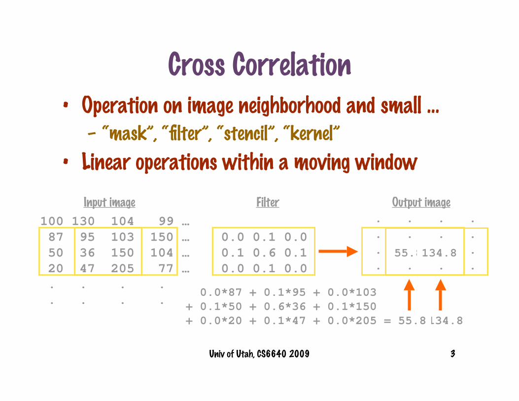
0.0*95 + 0.1*103 + 0.0*150+ 0.1*36 + 0.6*150 + 0.1*104+ 0.0*47 + 0.1*205 + 0.0*77 = 134.8
. . . . . . . . . . . . . . . .
100 130 104 99 … 87 95 103 150 … 50 36 150 104 … 20 47 205 77 … . . . . . . . .
Filter
0.0 0.1 0.00.1 0.6 0.10.0 0.1 0.0
Input image Output image
0.0*87 + 0.1*95 + 0.0*103+ 0.1*50 + 0.6*36 + 0.1*150+ 0.0*20 + 0.1*47 + 0.0*205 = 55.8
Cross Correlation• Operation on image neighborhood and small …
– “mask”, “filter”, “stencil”, “kernel”
• Linear operations within a moving window
55.8134.8

Univ of Utah, CS6640 2009 4
Cross Correlation
• 1D
• 2D

Univ of Utah, CS6640 2009 5
Correlation: Technical Details
• Boundary conditions– Pad image with amount (a,b)
• Constant value or repeat edge values
– Cyclical boundary conditions• Wrap or mirroring

Univ of Utah, CS6640 2009 6
Correlation: Technical Details
• Boundaries– Can also modify kernel – no long correlation
• For analysis– Image domains infinite
– Data compact (goes to zero far away from origin)

Univ of Utah, CS6640 2009 7
Correlation: Properties
• Shift invariant
• Linear
Compact notation

Univ of Utah, CS6640 2009 8
Filters: Considerations
• Normalize– Sums to one
– Sums to zero (some cases, later)
• Symmetry– Left, right, up, down
– Rotational
• Special case: auto correlation

Univ of Utah, CS6640 2009 9
0 0 00 1 00 0 0
1 1 11 1 11 1 1
1/9 *
Examples 1
Univ of Utah, CS6640 2009 10
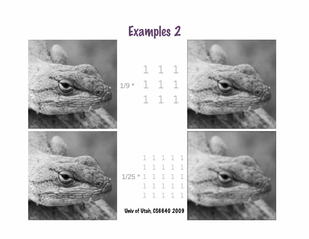
1 1 11 1 11 1 1
1 1 1 1 11 1 1 1 11 1 1 1 11 1 1 1 11 1 1 1 1
1/9 *
1/25 *
Examples 2
Univ of Utah, CS6640 2009 11
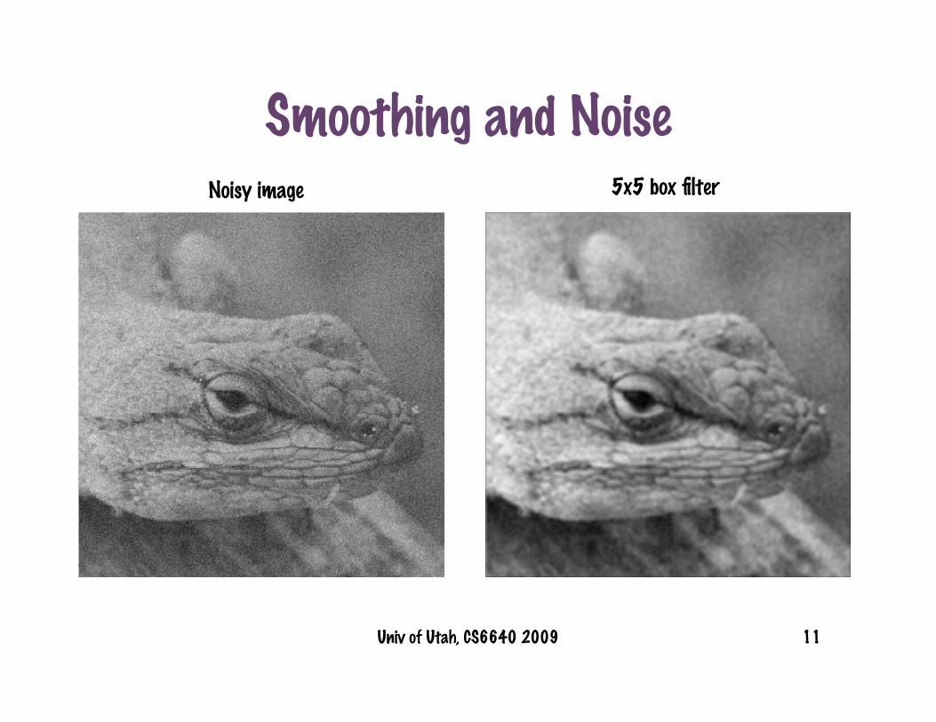
Smoothing and NoiseNoisy image 5x5 box filter
Univ of Utah, CS6640 2009 12
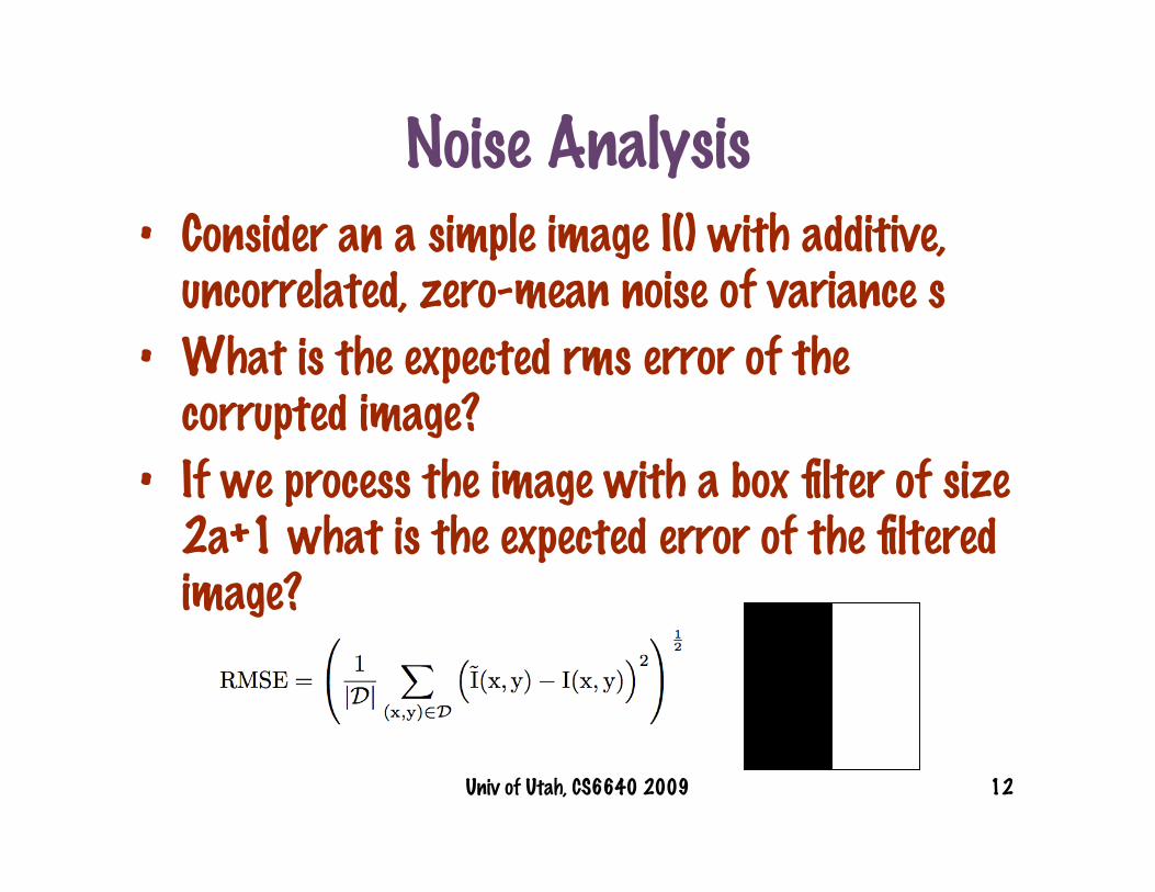
Noise Analysis• Consider an a simple image I() with additive,
uncorrelated, zero-mean noise of variance s
• What is the expected rms error of thecorrupted image?
• If we process the image with a box filter of size2a+1 what is the expected error of the filteredimage?
Univ of Utah, CS6640 2009 13
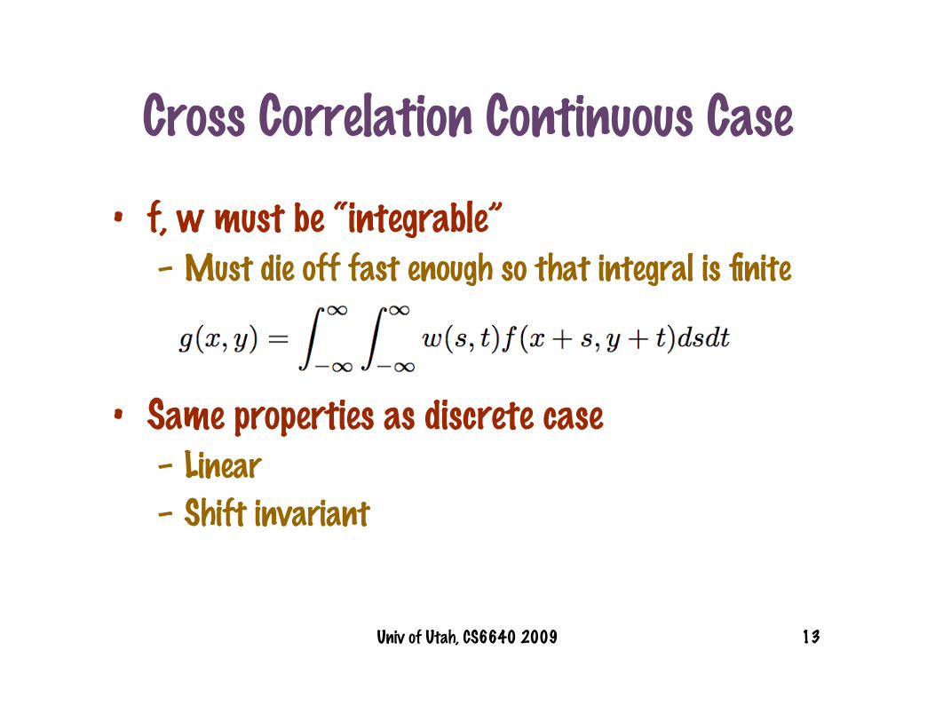
Cross Correlation Continuous Case
• f, w must be “integrable”– Must die off fast enough so that integral is finite
• Same properties as discrete case– Linear
– Shift invariant
Univ of Utah, CS6640 2009 14
Other Filters
• Disk– Circularly symmetric, jagged in discrete case
• Gaussians– Circularly symmetric, smooth for large enough
stdev– Must normalize in order to sum to one
• Derivatives – discrete/finite differences– Operators
Univ of Utah, CS6640 2009 15
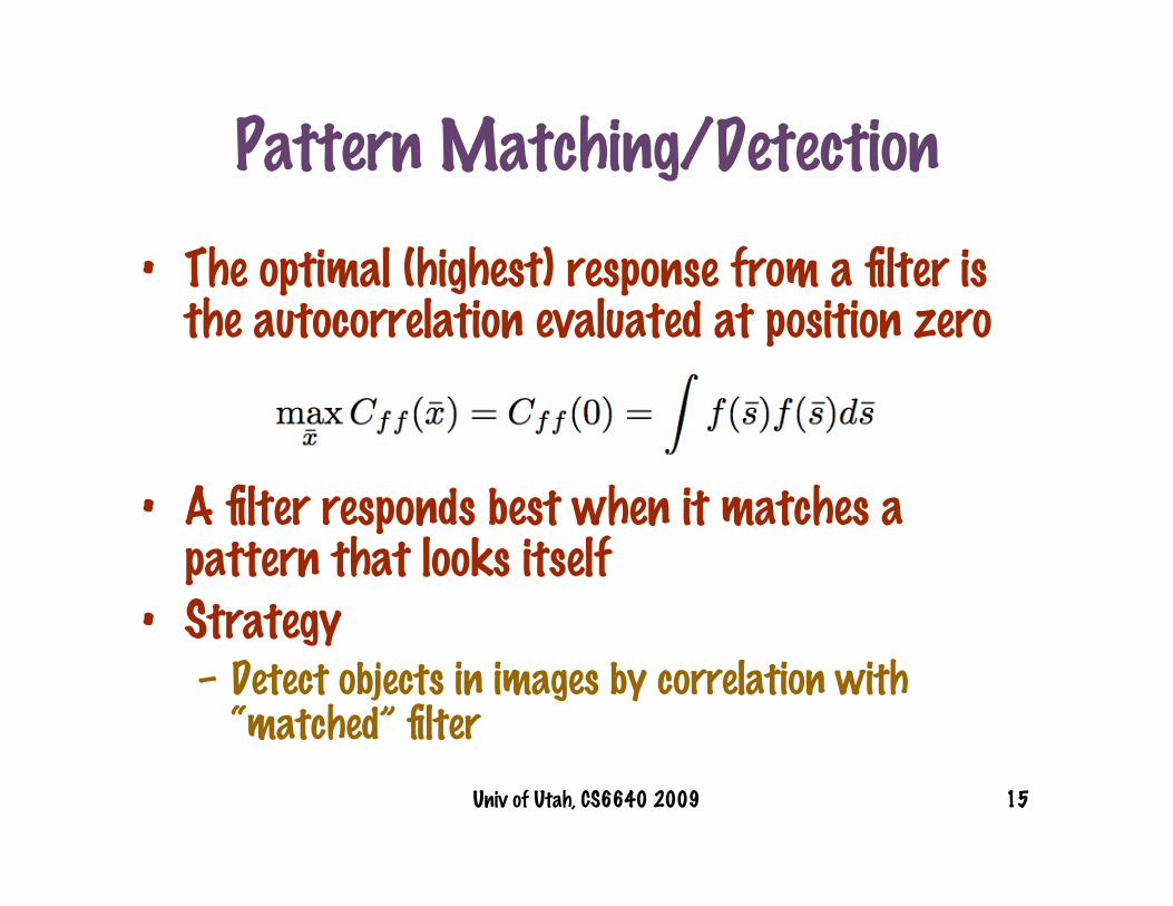
Pattern Matching/Detection
• The optimal (highest) response from a filter isthe autocorrelation evaluated at position zero
• A filter responds best when it matches apattern that looks itself
• Strategy– Detect objects in images by correlation with
“matched” filter

Univ of Utah, CS6640 2009 16
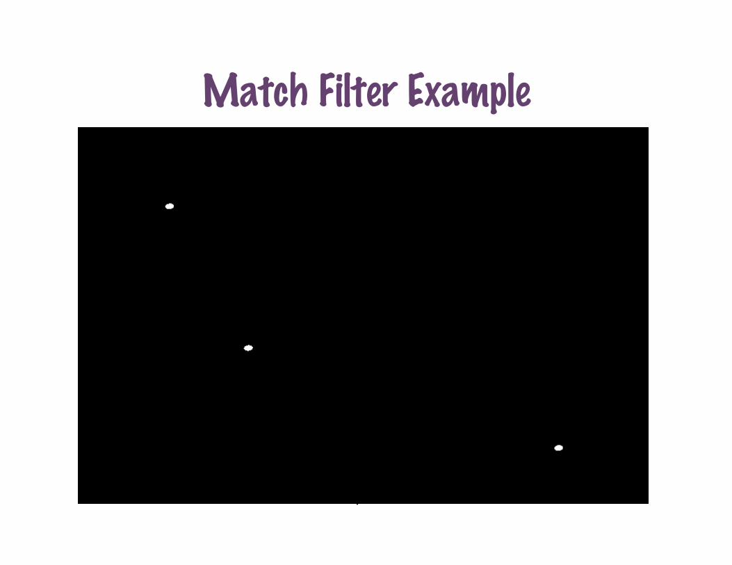
Match Filter Example
Trick: make surekernel sums tozero

Univ of Utah, CS6640 2009 17
Match Filter Example
Univ of Utah, CS6640 2009 18
Match Filter Example
Univ of Utah, CS6640 2009 19
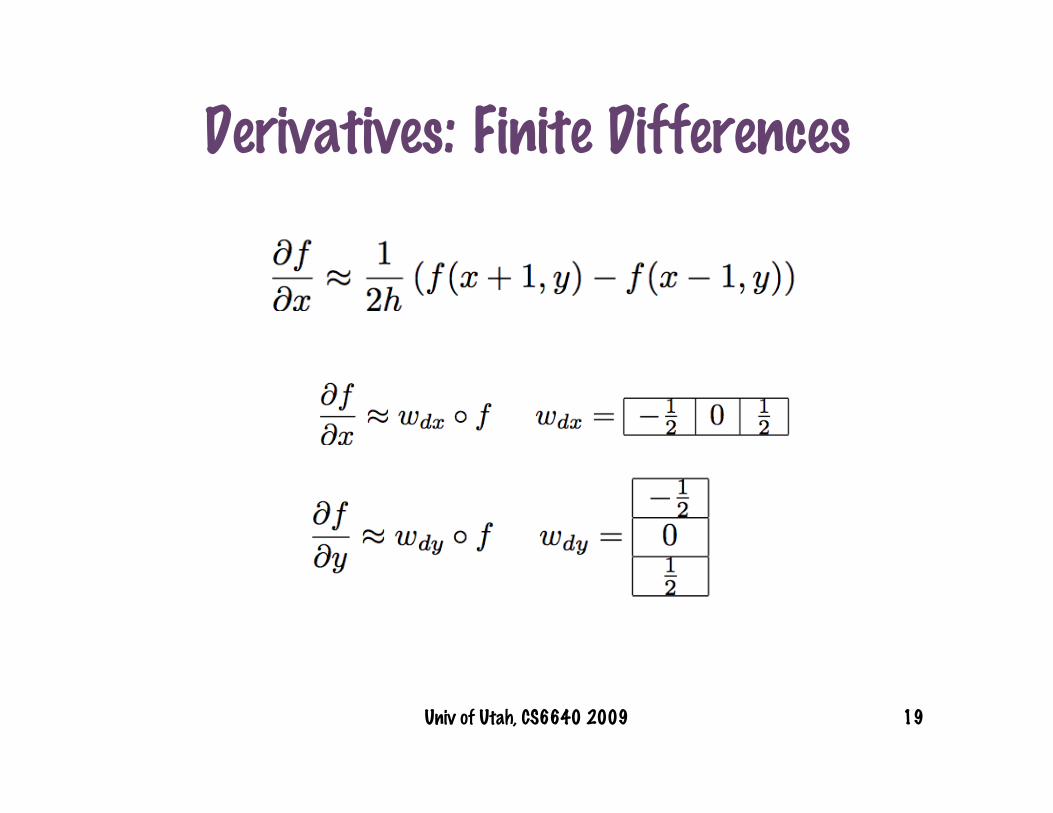
Derivatives: Finite Differences
Univ of Utah, CS6640 2009 20
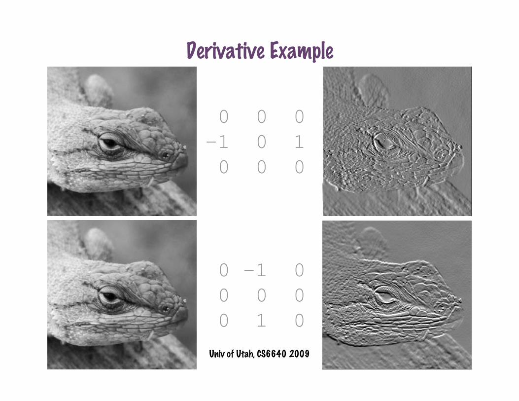
0 -1 0 0 0 0 0 1 0
0 0 0-1 0 1 0 0 0
Derivative Example
Univ of Utah, CS6640 2009 21
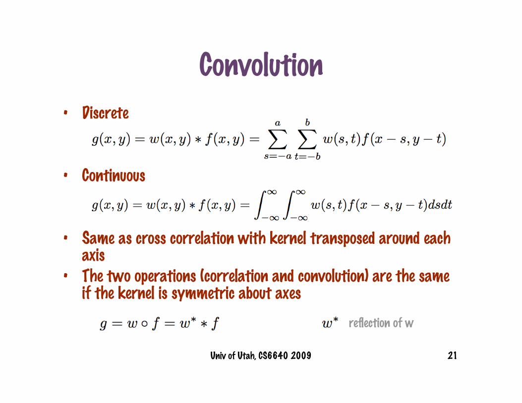
• Discrete
• Continuous
• Same as cross correlation with kernel transposed around eachaxis
• The two operations (correlation and convolution) are the sameif the kernel is symmetric about axes
Convolution
reflection of w

Univ of Utah, CS6640 2009 22
Convolution: Properties
• Shift invariant, linear• Cummutative
• Associative
• Others (discussed later):– Derivatives, convolution theorem, spectrum…

Univ of Utah, CS6640 2009 23
Computing Convolution
• Compute time– MxM mask
– NxN image
• Special case: separable
O(M2N2) “for” loops are nested 4 deep
O(M2N2) O(MN2)
Two 1D kernels
= *
Univ of Utah, CS6640 2009 24
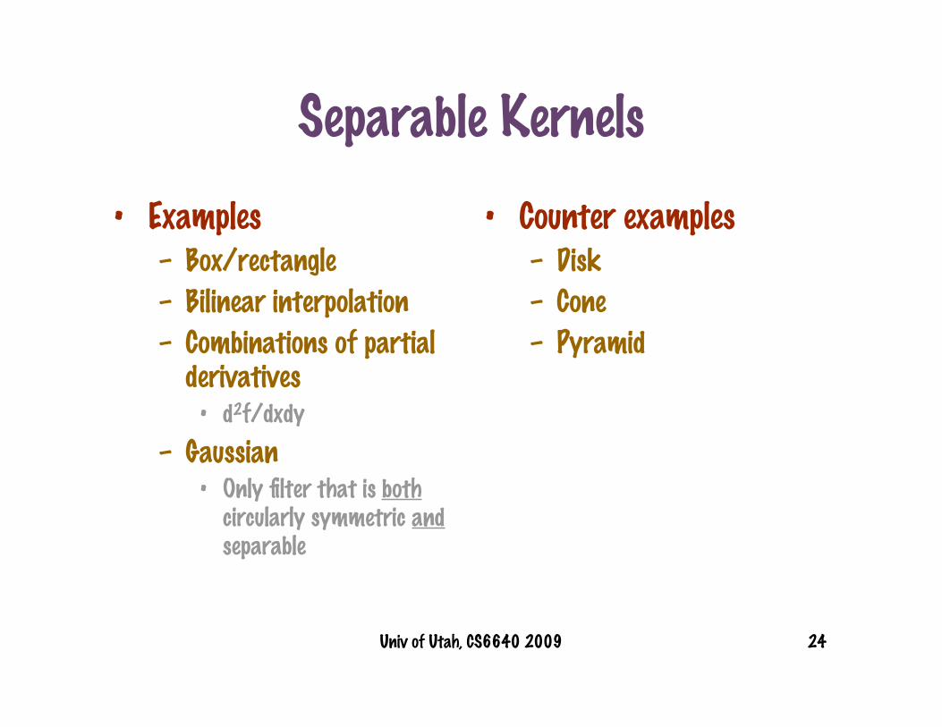
Separable Kernels
• Examples– Box/rectangle
– Bilinear interpolation
– Combinations of partialderivatives
• d2f/dxdy
– Gaussian• Only filter that is both
circularly symmetric andseparable
• Counter examples– Disk
– Cone
– Pyramid

Univ of Utah, CS6640 2009 25
Nonlinear Methods For Filtering
• Median filtering
• Bilateral filtering
• Neighborhood statistics and nonlocal filtering

Univ of Utah, CS6640 2009 26
Median Filtering
• For each neighborhood in image– Sliding window– Usually odd size (symmetric) 5x5, 7x7,…
• Sort the greyscale values• Set the center pixel to the median• Important: use “Jacobi” updates
– Separate input and output buffers– All statistics on the original image old new
Univ of Utah, CS6640 2009 27
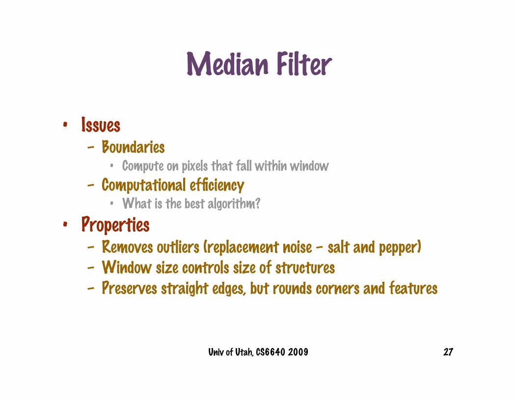
Median Filter
• Issues– Boundaries
• Compute on pixels that fall within window
– Computational efficiency• What is the best algorithm?
• Properties– Removes outliers (replacement noise – salt and pepper)– Window size controls size of structures– Preserves straight edges, but rounds corners and features

Univ of Utah, CS6640 2009 28
Median vs Gaussian
Original + GaussianNoise
3x3 Box3x3 Median

Univ of Utah, CS6640 2009 29
Replacement Noise• Also: “shot noise”, “salt&pepper”
• Replace certain % of pixels with samples from pdf
• Best strategy: filter to avoid outliers
Univ of Utah, CS6640 2009 30
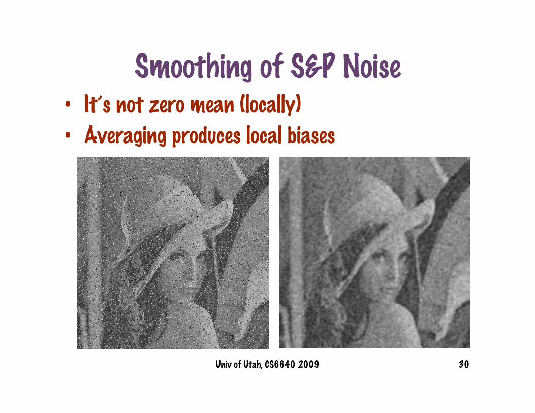
Smoothing of S&P Noise• It’s not zero mean (locally)
• Averaging produces local biases
Univ of Utah, CS6640 2009 31
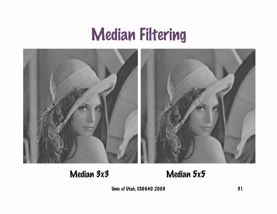
Median Filtering
Median 5x5Median 3x3

Univ of Utah, CS6640 2009 32
Median Filtering
Median 5x5Median 3x3

Univ of Utah, CS6640 2009 33
Median Filtering• Iterate
Median 3x3 2x Median 3x3

Univ of Utah, CS6640 2009 34
Median Filtering
• Image model: piecewise constant (flat)
Ordering
Output
Ordering
Output

Univ of Utah, CS6640 2009 35
Order Statistics• Median is special case of order-statistics filters
• Instead of weights based on neighborhoods, weights are basedon ordering of data
Neighborhood Ordering
Filter
Neighborhood average (box) Median filter
Trimmed average (outlier removal)
Univ of Utah, CS6640 2009 36
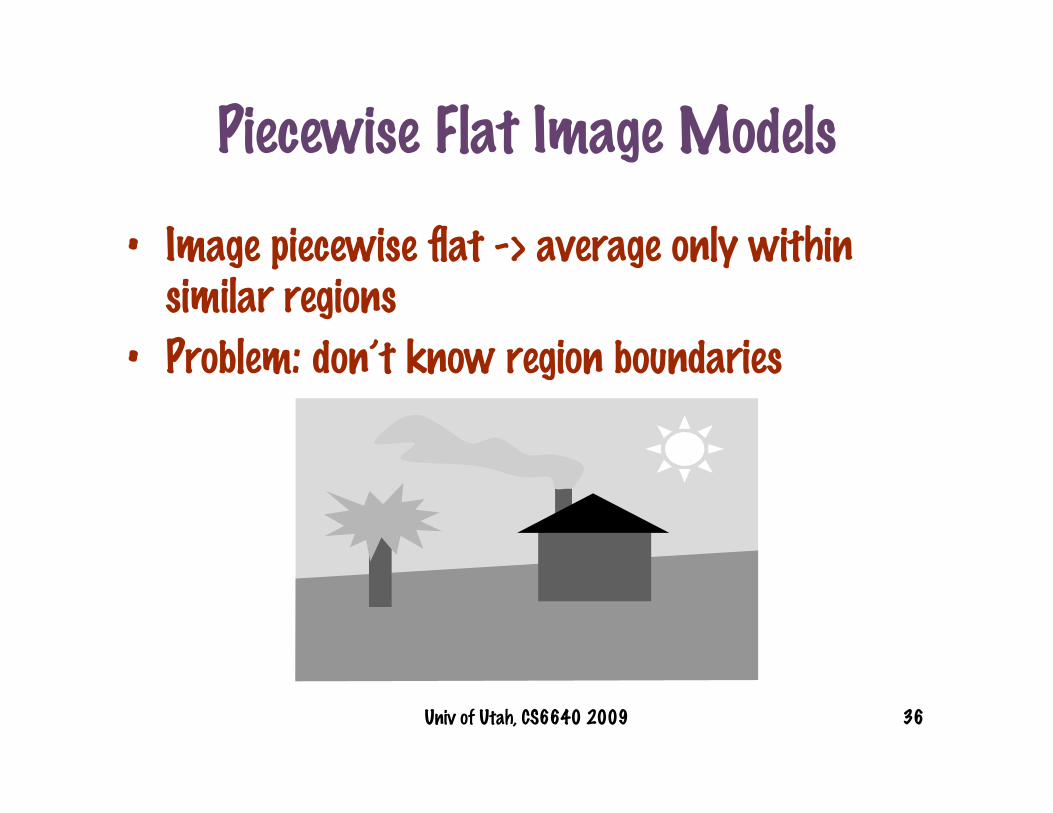
Piecewise Flat Image Models
• Image piecewise flat -> average only withinsimilar regions
• Problem: don’t know region boundaries
Univ of Utah, CS6640 2009 37
Piecewise-Flat Image Models
• Assign probabilities to other pixels in the imagebelonging to the same region
• Two considerations– Distance: far away pixels are less likely to be same
region
– Intensity: pixels with different intensities are lesslikely to be same region
Univ of Utah, CS6640 2009 38
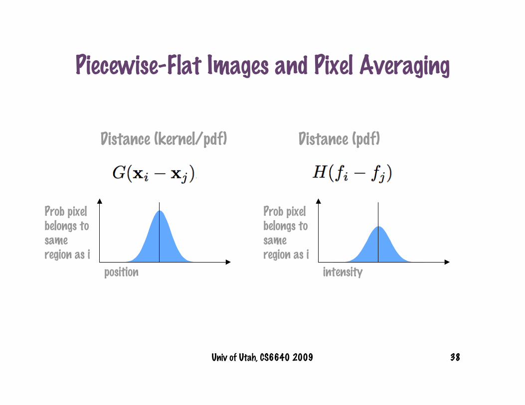
Piecewise-Flat Images and Pixel Averaging
Distance (kernel/pdf) Distance (pdf)
Prob pixelbelongs tosameregion as i
Prob pixelbelongs tosameregion as i
intensityposition

Univ of Utah, CS6640 2009 39
• Neighborhood – sliding window• Weight contribution of neighbors according to:
• G is a Gaussian (or lowpass), as is H, N is neighborhood,– Often use G(rij) where rij is distance between pixels– Update must be normalized for the samples used in this (particular)
summation
• Spatial Gaussian with extra weighting for intensity– Weighted average in neighborhood with downgrading of intensity
outliers
Bilateral Filter

Univ of Utah, CS6640 2009 40
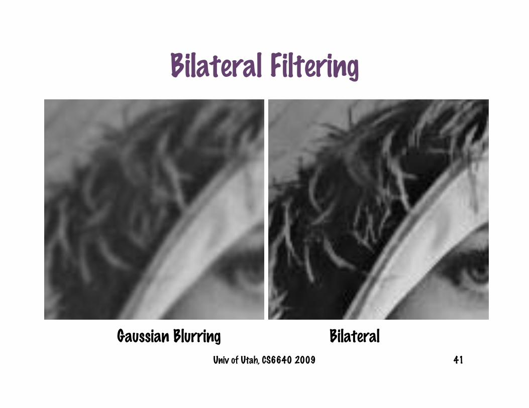
Bilateral Filtering
BilateralGaussian Blurring
Univ of Utah, CS6640 2009 41
Bilateral Filtering
BilateralGaussian Blurring

Univ of Utah, CS6640 2009 42
Nonlocal Averaging
• Recent algorithm– NL-means, Baudes et al., 2005– UINTA, Awate & Whitaker, 2005
• Different model– No need for piecewise-flat– Images consist of pixels with similar neighborhoods
• Scattered around– General area of a pixel– All around
• Idea– Average pixels with similar neighborhoods
Univ of Utah, CS6640 2009 43
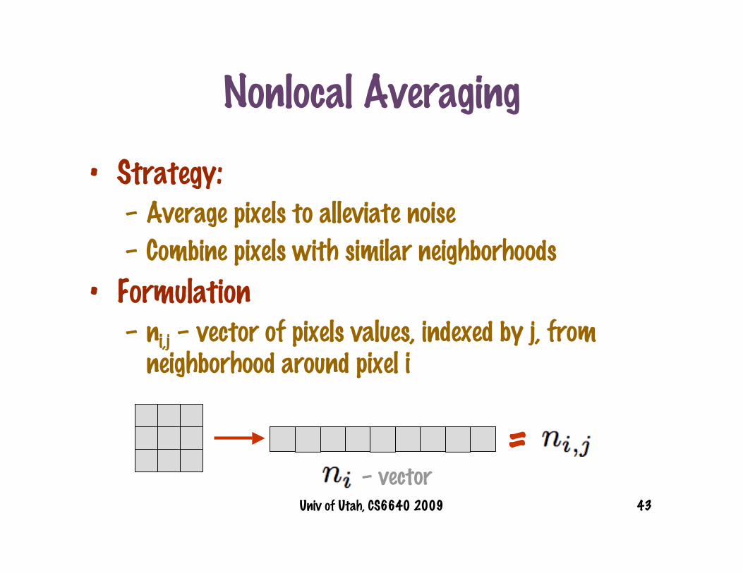
Nonlocal Averaging
• Strategy:– Average pixels to alleviate noise
– Combine pixels with similar neighborhoods
• Formulation– ni,j – vector of pixels values, indexed by j, from
neighborhood around pixel i
=– vector

Univ of Utah, CS6640 2009 44
Nonlocal Averaging Formulation
• Distance between neighborhoods
• Kernel weights based on distances
• Pixel values: fi

Univ of Utah, CS6640 2009 45
Averaging Pixels Based on Weights
• For each pixel, i, choose a set of pixel locations– j = 1, …., M
– Average them together based on neighborhoodweights

Univ of Utah, CS6640 2009 46
Nonlocal Averaging
Univ of Utah, CS6640 2009 47
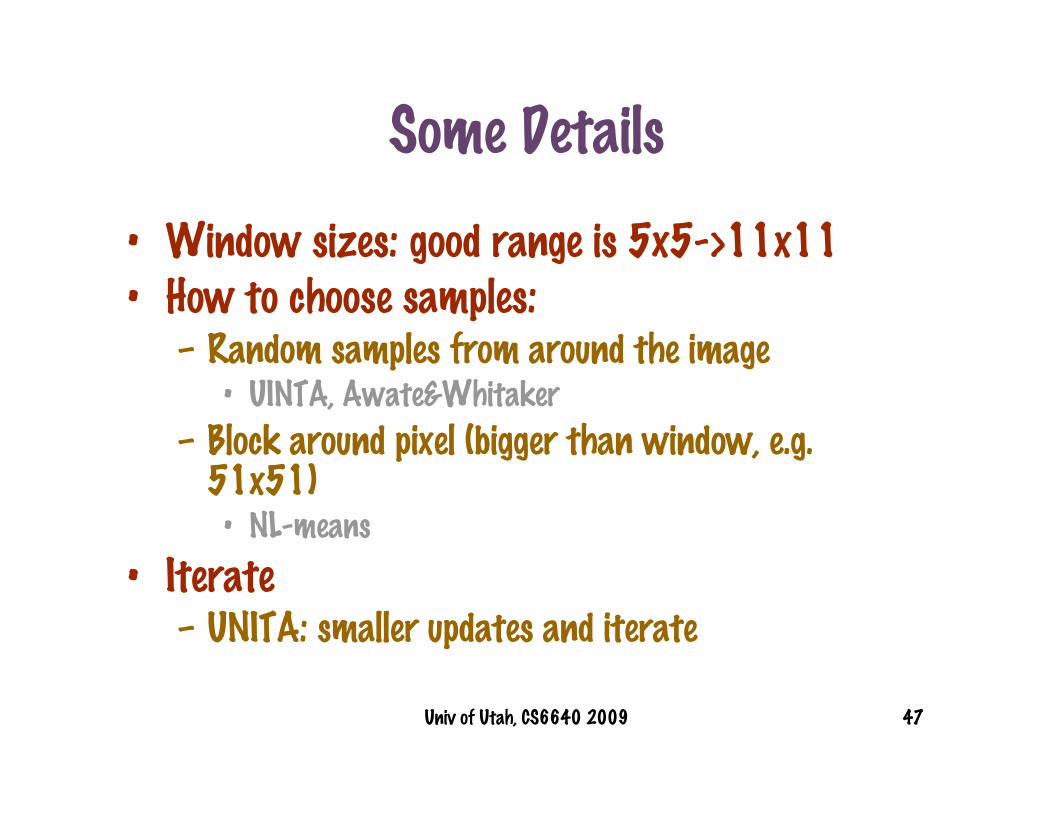
Some Details
• Window sizes: good range is 5x5->11x11• How to choose samples:
– Random samples from around the image• UINTA, Awate&Whitaker
– Block around pixel (bigger than window, e.g.51x51)
• NL-means
• Iterate– UNITA: smaller updates and iterate

Univ of Utah, CS6640 2009 48
NL-Means Algorithm
• For each pixel, p– Loop over set of pixels nearby
– Compare the neighorhoods of those pixels to theneighborhood of p and construct a set of weights
– Replace the value of p with a weighted combinationof values of other pixels
• Repeat… but 1 iteration is pretty good

Univ of Utah, CS6640 2009 49
Results
Noisy image (range 0.0-1.0) Bilateral filter (3.0, 0.1)
Univ of Utah, CS6640 2009 50
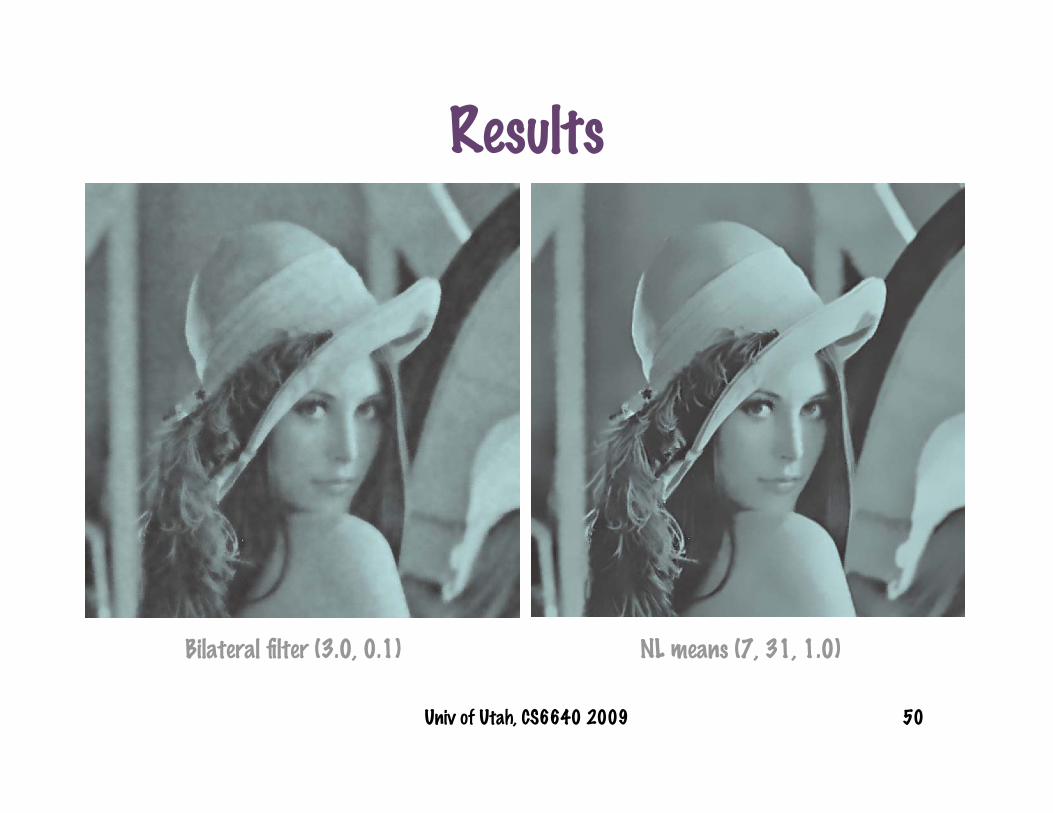
Results
Bilateral filter (3.0, 0.1) NL means (7, 31, 1.0)
Univ of Utah, CS6640 2009 51
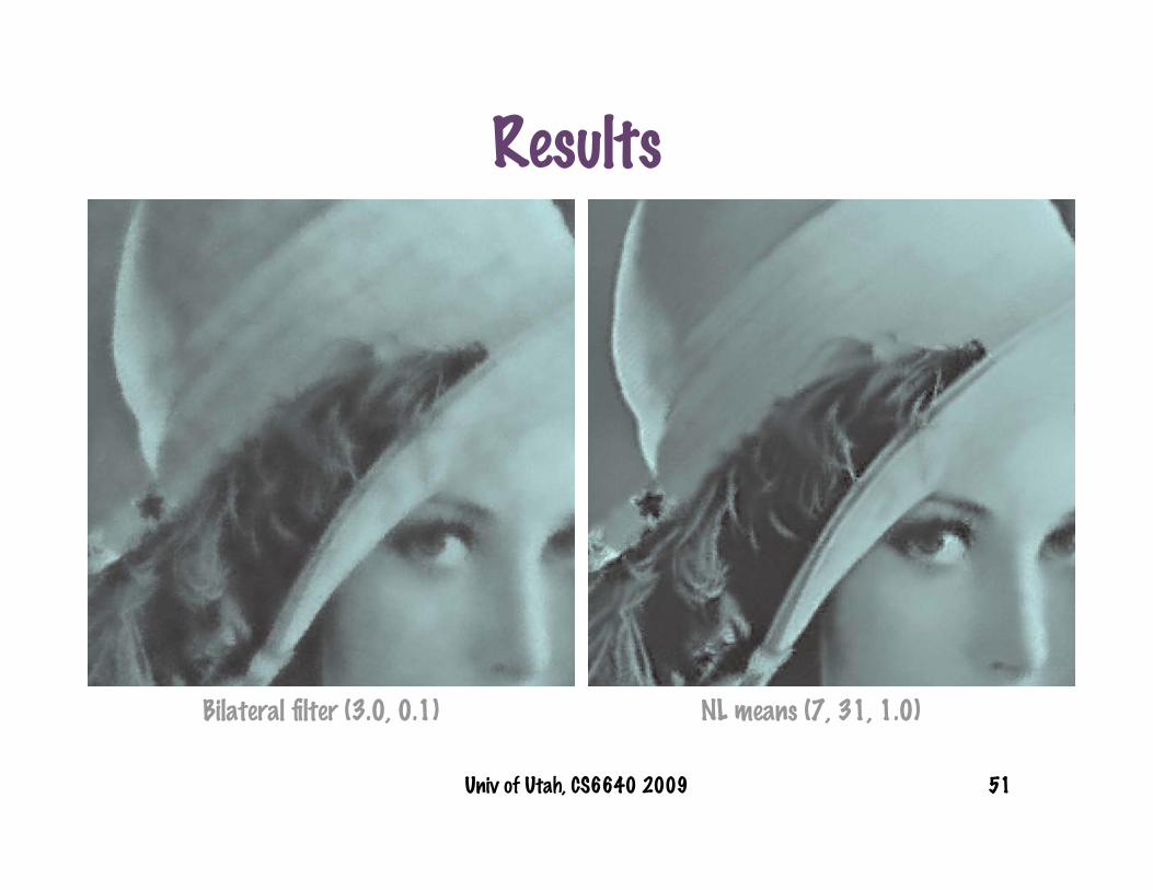
Results
Bilateral filter (3.0, 0.1) NL means (7, 31, 1.0)
Univ of Utah, CS6640 2009 52
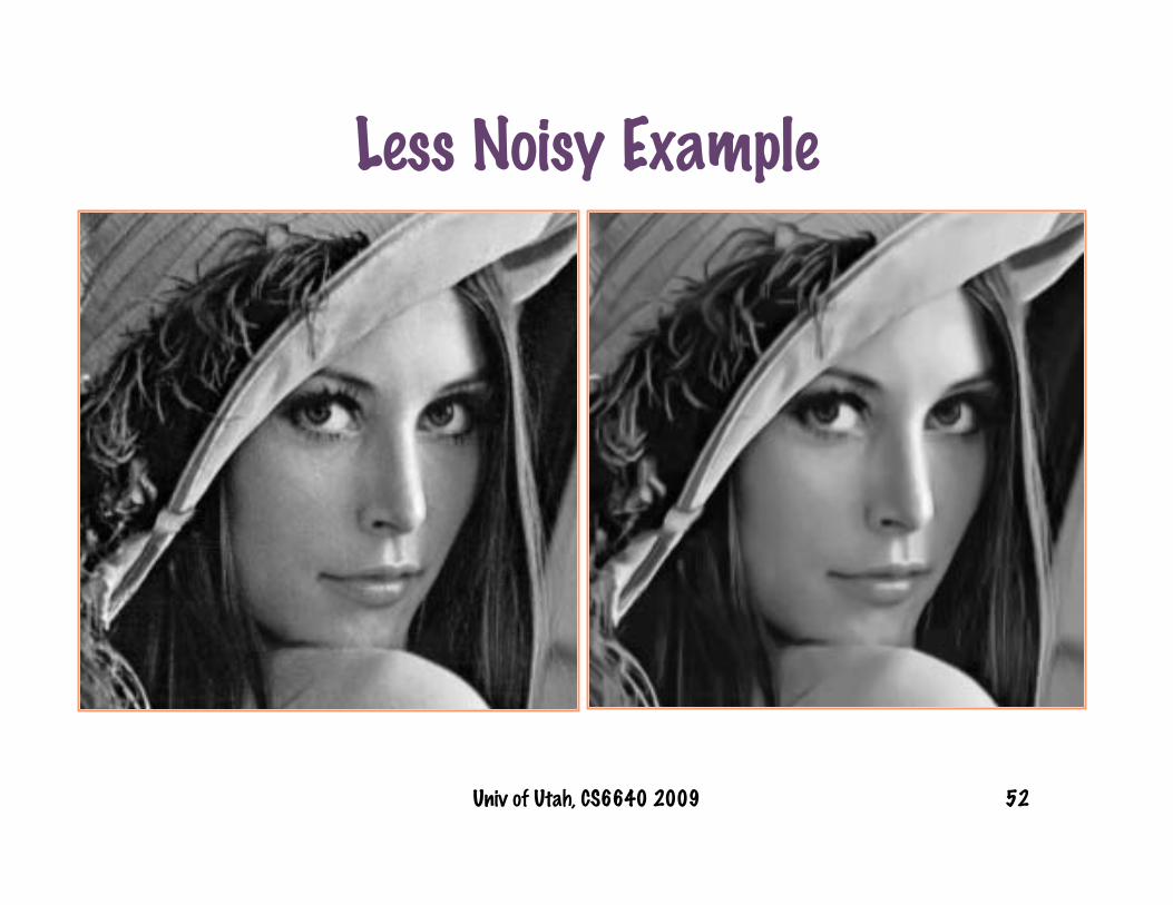
Less Noisy Example

Univ of Utah, CS6640 2009 53
Less Noisy Example

Univ of Utah, CS6640 2009 54
Results
Original Noisy Filtered

Univ of Utah, CS6640 2009 55
Checkerboard With Noise
Original Noisy Filtered
Univ of Utah, CS6640 2009 56
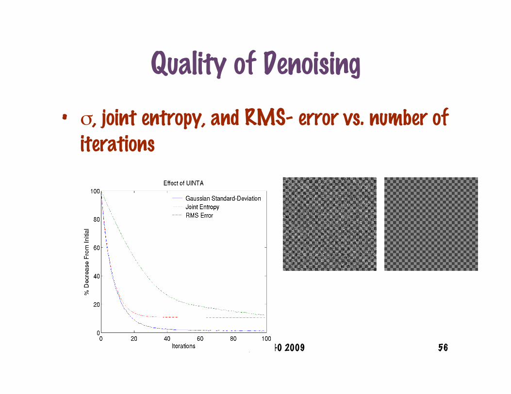
Quality of Denoising
• σ, joint entropy, and RMS- error vs. number ofiterations

Univ of Utah, CS6640 2009 57
MRI Head

Univ of Utah, CS6640 2009 58
MRI Head
Univ of Utah, CS6640 2009 59
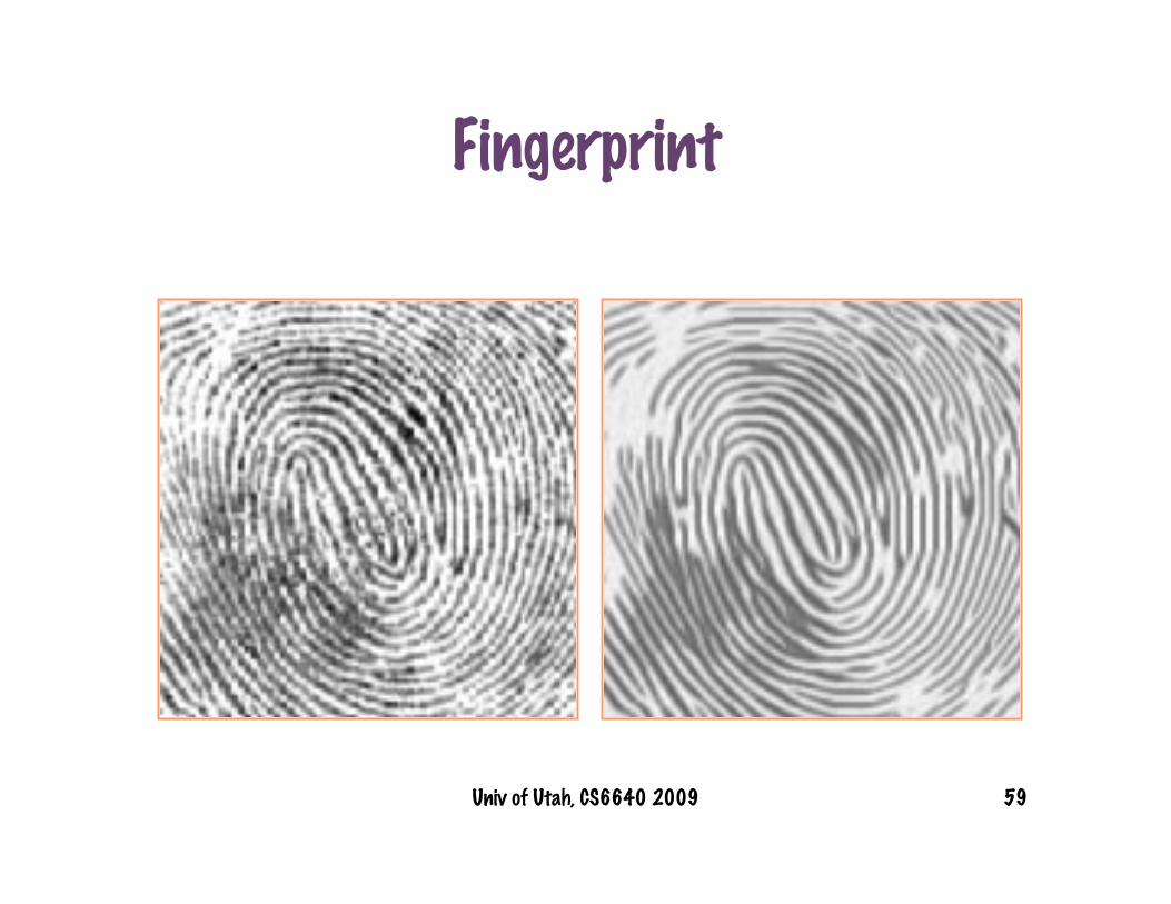
Fingerprint

Univ of Utah, CS6640 2009 60
Fingerprint
Univ of Utah, CS6640 2009 61
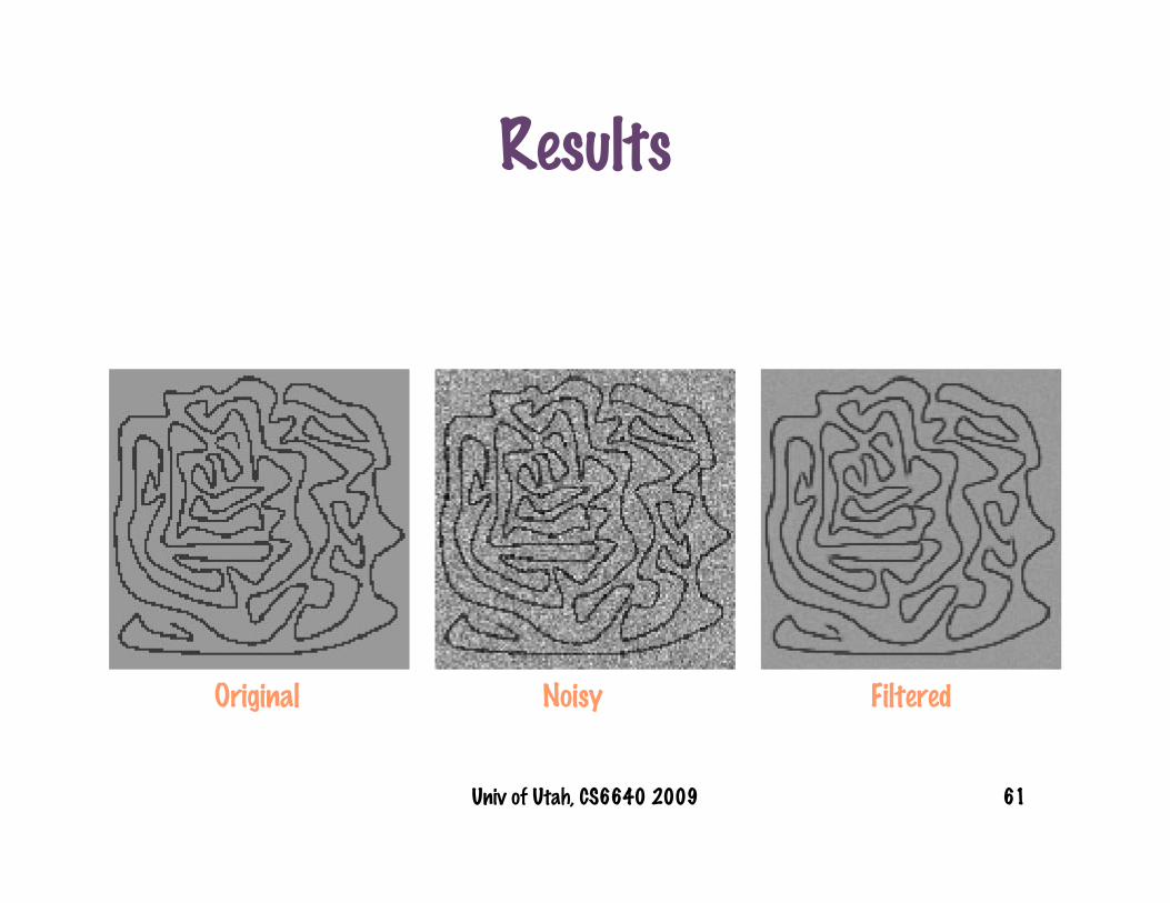
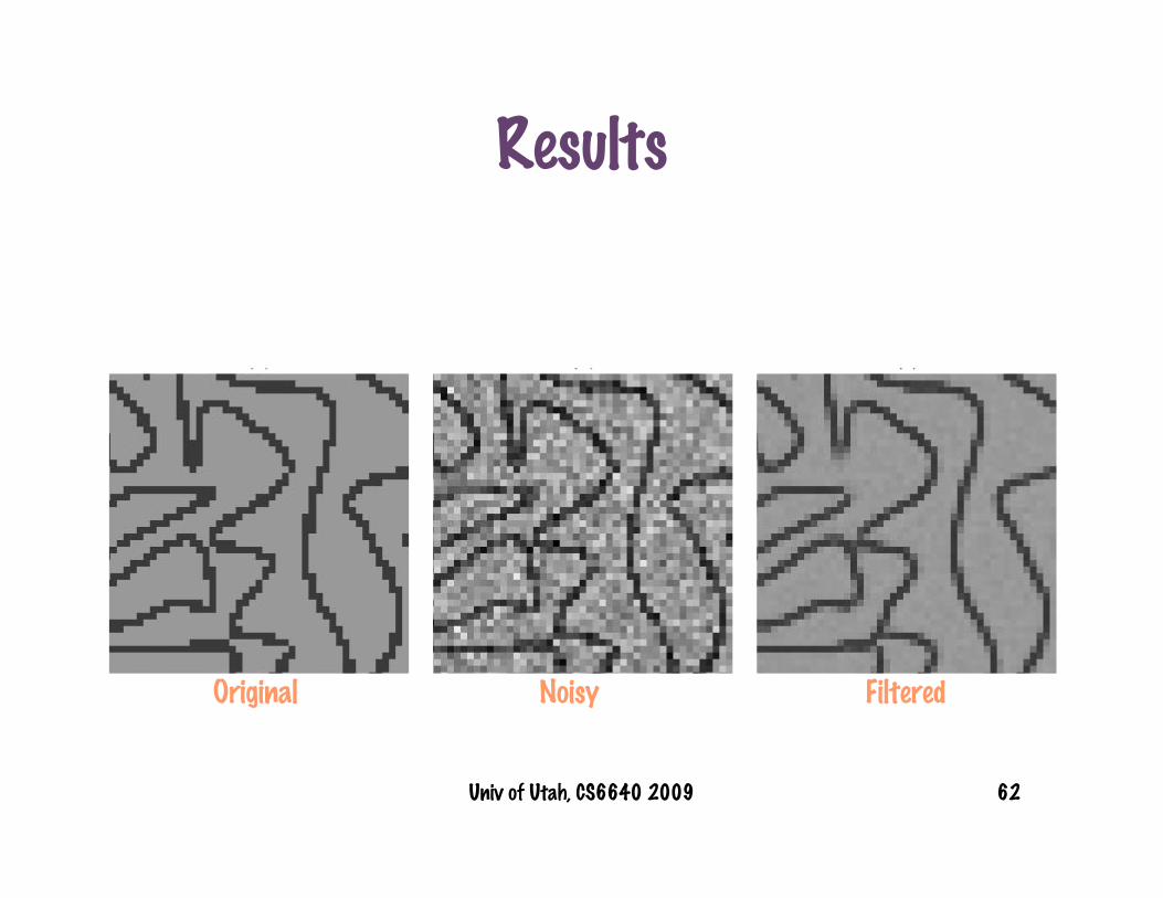
Results
Original Noisy Filtered
Univ of Utah, CS6640 2009 62
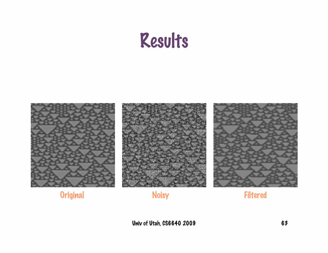
Results
Original Noisy Filtered
Univ of Utah, CS6640 2009 63
Results
Original Noisy Filtered

Univ of Utah, CS6640 2009 64
Fractal
Original Noisy Filtered
Univ of Utah, CS6640 2009 65
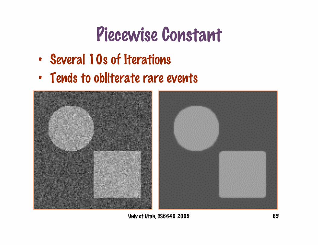
Piecewise Constant• Several 10s of Iterations
• Tends to obliterate rare events
Univ of Utah, CS6640 2009 66
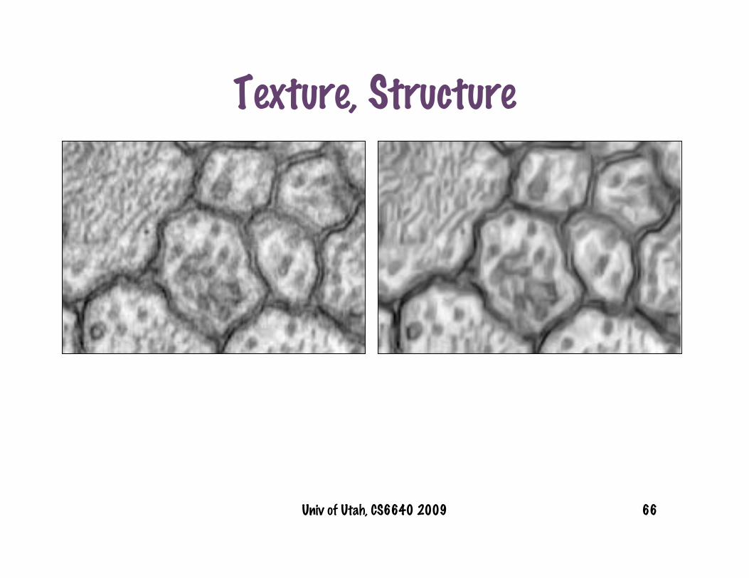
Texture, Structure
Univ of Utah, CS6640 2009 67