fig. 38 insensitivity of wake strength at high (g) numerical and...

(G) Numerical and Experimental Results

To begin, we shall show some data of

R. D. Moser, J. Kim & N. N. Mansour, “Direct numerical simulation of turbulent

flow up to Re! = 590,” Phys. Fluids 11 943-945 (1999)

as analyzed by Panton (2005). The first figure shows data for g0(y+) and the second for the

composite expansion of the stress

!u!v!

u2"

!!!comp

= g0(y+)! !

compared with the data. The third compares the composite expansion for the mean velocity

u(y)u"

!!!comp

= f0(y+) + W0(!)

directly with the data and, in the fourth plot, by the log-law “diagnostic function”

y+ "(u/u")"y+

!!!comp

= y+ df0(y+)dy+ + ! dW0(#)

d#

The expansions work less well for the mean-velocity which is not as highly constrained by the

RANS equations as in the stress.

The question of when one can observe a logarithmic portion in

the velocity profile is addressed by the diagnostic function !(y!):

!"y!du!

dy!(7.21)

A logarithmic portion is indicated when ! takes on the constantvalue !"1/". Figure 42 shows ! for the highest Re

*"590 Ames

channel flow data along with the ! computed for the compositeprofile shown in Fig. 41 with #"0.1. The DNS has no log portionwhile the composite predicts a log portion between y!"65 and95. A comparison of the ! predicted by the composite expansionfor channel flow Reynolds numbers of 500 and 1000 is displayedon Fig. 43. The higher Reynolds number in channel flow increases

the log portion to 65#y!#160.Figure 44 is a low-order composite expansion prediction for

boundary layer flow with #"0.60. In the boundary layer flow thelarger wake component completely obliterates the log portion atRe*

"500. At Re*

"1000 there is a small portion that is almostflat, 60#y!#85, but the level is ""0.379 rather then the value

assumed in the calculation, 0.390. At Re*

"5000 the curve showsa log region with a value ""0.3895. Very close to the 0.390 valueused in the calculation. The region where "$0.385 is located 60#y!#270. According to this model the log region of a boundarylayer begins about y!"60 and extends upward as the Reynoldsnumber increases.

Based on a low-order composite expansion, a log portion

should not be expected until reasonably high Re*are attained. A

larger wake component compounds this effect. This is consistentwith the conclusion of Osterlund et al $66% that significant loga-rithmic overlap is not seen until Re&"6000 'Re*"1500(.

7.5 Power Law Versus Log Law. I regard the issue ‘‘powerlaw versus log law’’ as an artificial question. From the viewpointof composite expansions, the log law is the common part of the

inner and outer functions. It is the limiting form of f as y!!)and of F as Y!0. In principle it is not an equation that approxi-mates the data, the composite expansion theoretically has thatrole. At high enough Re

*the velocity profile does show a neigh-

borhood where the log law is a reasonable data approximation.

Fig. 38 Insensitivity of wake strength at highRe*. Data of Smith and Walker †99‡ correctedby East et al †72‡.

Fig. 39 Reynolds stress wall function forAmes channel flow DNS. Data from Moser et al†102‡.

Applied Mechanics Reviews JANUARY 2005, Vol. 58 Õ 27

Downloaded 21 Apr 2008 to 128.220.254.4. Redistribution subject to ASME license or copyright; see http://www.asme.org/terms/Terms_Use.cfm

Fig. 39 Reynolds stress wall function for Ames channel flow DNS.

.

61

This is easier to observe in pipe flow than in boundary layersflows because pipe flows have a small wake component.Consider the analogous question for the Reynolds stress. The

common part is !!uv"/u*2 "1. Is the value unity a good approxi-

mation for !!uv"/u*2 in some neighborhood of y#? Not really.

At Re*

"10,000 the maximum is !!uv"/u*2 "0.97, 3% low. One

could fit a parabola at the maximum point

ymax# #!Re

*$

(7.22)

!!uv"maxu*2

#1!2

!$ Re*

(7.23)

The parabola would fit much better, however, it would have sev-eral ‘‘constants’’ that depend on the Reynolds number. In essenceit would be a curve fit with no theoretical significance.As noted in the introduction Prandtl used a power law as an

approximating equation for Reynolds numbers less thanUaveD/%$100,000. He assumed a friction law &with power lawform' to derive the power law U/u*"C(y#)n with n"1/7 and Cconstant. Engineers have used a power law anchored at the center,

U/U0"Yn where n is a function of Reynolds number. Theseequations have always been regarded as curve fits.

Barenblatt asserts that a power law is theoretically well-founded and superior the log law for approximating pipe flowvelocity profiles. This idea is presented in his first book, Barenb-latt (25) as a alternative to the log law. In more recent articles, hispower law is claimed to be superior to the log law &Barenblattet al (28–30)'. Specifically he advocates the relation

U&y '

u*

"Cy#n (7.24)

where the coefficients are functions of the pipe Reynolds number,Red :

n&Red'"a

ln Red"

3/2

ln Red(7.25)

C&Red'"b#c ln Red"1

!3#5

2ln Red (7.26)

The choice of the coefficients a, b, and c was based on Ni-kuradse’s data.Barenblatt does not intend that Eq. &7.24' is valid in the center

of the pipe or near the wall.

Barenblatt’s equations have been plotted for Re*"103, 104,105 and 106 on Figs. 45 and 46 in different forms. In the first

Fig. 40 Composite expansion for Reynoldsstress and Ames channel flow DNS. Data fromMoser et al †102‡.

Fig. 41 Composite expansion for velocity andAmes channel flow DNS at Re*Ä590. Data fromMoser et al †102‡.

28 Õ Vol. 58, JANUARY 2005 Transactions of the ASME


Fig. 40 Composite expansion for Reynolds stress and Ames channel flow DNS.

This is easier to observe in pipe flow than in boundary layersflows because pipe flows have a small wake component.Consider the analogous question for the Reynolds stress. The

common part is !!uv"/u*2 "1. Is the value unity a good approxi-

mation for !!uv"/u*2 in some neighborhood of y#? Not really.

At Re*

"10,000 the maximum is !!uv"/u*2 "0.97, 3% low. One

could fit a parabola at the maximum point

ymax# #!Re

*$

(7.22)

!!uv"maxu*2

#1!2

!$ Re*

(7.23)

The parabola would fit much better, however, it would have sev-eral ‘‘constants’’ that depend on the Reynolds number. In essenceit would be a curve fit with no theoretical significance.As noted in the introduction Prandtl used a power law as an

approximating equation for Reynolds numbers less thanUaveD/%$100,000. He assumed a friction law &with power lawform' to derive the power law U/u*"C(y#)n with n"1/7 and Cconstant. Engineers have used a power law anchored at the center,

U/U0"Yn where n is a function of Reynolds number. Theseequations have always been regarded as curve fits.

Barenblatt asserts that a power law is theoretically well-founded and superior the log law for approximating pipe flowvelocity profiles. This idea is presented in his first book, Barenb-latt (25) as a alternative to the log law. In more recent articles, hispower law is claimed to be superior to the log law &Barenblattet al (28–30)'. Specifically he advocates the relation

U&y '

u*

"Cy#n (7.24)

where the coefficients are functions of the pipe Reynolds number,Red :

n&Red'"a

ln Red"

3/2

ln Red(7.25)

C&Red'"b#c ln Red"1

!3#5

2ln Red (7.26)

The choice of the coefficients a, b, and c was based on Ni-kuradse’s data.Barenblatt does not intend that Eq. &7.24' is valid in the center

of the pipe or near the wall.

Barenblatt’s equations have been plotted for Re*"103, 104,105 and 106 on Figs. 45 and 46 in different forms. In the first

Fig. 40 Composite expansion for Reynoldsstress and Ames channel flow DNS. Data fromMoser et al †102‡.

Fig. 41 Composite expansion for velocity andAmes channel flow DNS at Re*Ä590. Data fromMoser et al †102‡.

28 Õ Vol. 58, JANUARY 2005 Transactions of the ASME


Fig. 41 Composite expansion for velocity and Ames channel flow DNS at Re!=590.

62

figure the difference between the power law and the log law is

plotted as a function of y!. The log law coefficients used arethose recommended by Barenblatt !26"; #"0.40 and Ci"5.1. Thepower law starts at a level higher than the log law, comes down

below the log law by about u!"#0.5 and then rises. Choosingdifferent constants # and Ci could make the power law curvesvery closely tangent to the log law, however, this decreases the

approximating ability at larger distances. As the Reynolds number

increases, the region where the power law comes close to the log

law moves outward. Thus, the region of invalidity near the wall

increases in size as Reynolds number increases. But, this invalid

region is in terms of y!.

In Fig. 46 the difference curves are plotted as a function of Y.

This is essentially a wake representation and Coles wake law is

shown for comparison. The power law mimics the first portion of

the wake law and this approximation is better at higher Reynolds

numbers. The power law does not produce a wake component that

is independent of Reynolds number. The major point of Figs. 45

and 46 is that the power law mimics the outer part of the log law

and the beginning of the wake law. When the center of the pipe is

reached, the power law has its maximum slope. There is a region,

especially at high Reynolds numbers, where the power law

roughly approximates $$0.5% the data. The region of a reasonablygood fit is probably larger than that of the log law. However, the

log law is not an approximating formula. In principle the compari-

son should be made with the log law plus the wake law.

The authors of recent pipe flow measurements, Zagarola and

Smits !54" and Toonder and Nieuwstadt !104", have been asked tocompare their data to the power law. Neither set of authors con-

cludes that the power law is a superior representation. Now con-

cerning the claim that the power law has theoretical foundations.

Barenblatt begins his derivation from the equation

Fig. 42 Log law diagnostic function gamma for channel flow.Composite expansion and Ames DNS at Re*Ä590.

Fig. 43 Log law diagnostic function gammafor channel flow. Composite expansion atRe*Ä500 and 1000.

Fig. 44 Log law diagnostic function gammafor boundary layer. Composite expansion atRe*Ä500, 1000, and 5000.

Applied Mechanics Reviews JANUARY 2005, Vol. 58 Õ 29


The same quantity has been analyzed in more recent simulations of

S. Hoyas & J. Jimenez, “Scaling of the velocity fluctuations in turbulent channels

up to Re! = 2003,” Phys. Fluids 18 011702 (2006)

by

J. Jimenez & R. D. Moser, “What are we learning from simulating wall turbulence?”

Philos. Trans. Roy. Soc. A 365 715-732 (2007).

In the first figure, the diagnostic function is plotted in both inner and outer scalings. No clear

plateau is observed. In the second figure a comparison is made with the next-order matched

asymptotics of

N. Afzal & K. Yajnik, “Analysis of turbulent pipe and channel flows at moderately

large Reynolds number,” J. Fluid Mech. 61 23-31 (1973)

which leads to the prediction

y "(u/u")"y = 1

$ + " y+

Re"+ %

Re"

or

y "(u/u")"y = 1

$ + "! + %Re"

63

The agreement seems good with " = 1.0, # = 150, when compared with the DNS and also

experiments of

V. K. Natrajan & K. T. Christansen, “The role of coherent structures in subgrid-

scale energy transfer within the log-layer of wall turbulence,” Phys. Fluids 18

065104 (2006)

refined overlap expressions:

uCi Z

1

kC

b

hC

! "ln yCC

ayC

hCCBi; !4:6"

uCo KuC

c Z1

kC

b

hC

! "ln ~yCa~yCBo: !4:7"

In the context of this analysis, the integration constants Bi and B0 are, ingeneral, Reynolds number-dependent, though k, a and b are not. However, thedata presented below indicates that this Reynolds number dependence shouldnot be strong.

A nearly identical result was obtained by Afzal & Yajnik (1973), though theyretained the possibility of a non-zero f0, by allowing F1 to be singular at zero,which is not considered here because it violates our assumptions of the regularityof the functions at zero. However, such a singular term could arise if a y shift isintroduced in the logarithmic law (Lindgren et al. 2004), which might extend therange of validity of the representation to somewhat smaller y. This possibilitywill not be explored here.

To evaluate the validity of the finite Reynolds number refinement of thelogarithmic law described above, numerical simulations (del Alamo et al. 2004;Hoyas & Jimenez 2006) are used to determine the quantity y!duC=dy", which isplotted versus yC and ~y in figure 6. According to the above analysis, expressionsfor this quantity in inner and outer coordinates are

yvuC

vyZ

1

kC

ayC

hCC

b

hC; !4:8"

yvuC

vyZ

1

kCa~yC

b

hC: !4:9"

In the overlap region where these expressions apply, y!vuC=vy", which wouldbe a constant with value 1/k in a log-layer, will be a line with slope of a/hC whenplotted in inner units. In this way, a log-layer is approached at high hC asthe slope of y!vuC=vy" goes to zero in the overlap. In outer units, the slope ofy!vuC=vy" in the overlap region is independent of hC. In figure 6, it appears thatthe hCZ940 and hCZ2000 channels exhibit a straight region with these

0 500 1000 1500 20002.0

2.5

3.0

3.5

4.0(a) (b)

9405502000

y+

ydu+

dy

0 0.2 0.4 0.6 0.8 1.02.0

2.5

3.0

3.5

4.0

9405502000

y

Figure 6. yduC/dy from direct numerical simulation at hCZ550, 940 and 2000.

725Study of turbulence near walls

Phil. Trans. R. Soc. A (2007)

properties for ~y!0:45 and yCO300, which are thus the limits of applicability ofthe overlap expressions (4.8) and (4.9). The slope of the curves in the overlapregion is az1.0, which is estimated from the hCZ2000 case.

These limits are much larger than those commonly assumed and discussed in §2.However, recent experiments also suggest amuch larger inner limit for the log layer,ranging from yCw200 to 600 (Osterlund et al. 2000; Zanoun et al. 2003; McKeonet al. 2004). Further in Wosnik et al. (2000), a Reynolds number-dependentmesolayer in the range 30!hC!300 is postulated, with a log layer only evidentbeyond yCw300, and Lindgren et al. (2004) propose that the apparent log layerbreaks down for yC!200 owing to a y offset in the logarithmic term.

The extension of the outer limit of the overlap representation to ~yz0:45 issomewhat surprising, but it may be that including the next order term expandsthe range of applicability. For example, in the overlap range, the value ofy!duC=dy", which can be considered the local value of 1/k, varies byapproximately 20% (independent of hC). If one insisted on a region withnegligible variation of k (i.e. a true logarithmic layer), one would likely choose amore limited range of ~y.

The values of k and b in the channel are estimated from the numerical simulationprofiles at hCZ940 and2000 (figure 7a).The lines describedby (4.8) intersect at thepoint yCZKb/azK150, y!duC=dy"Z1=kz2:49. The parameters are thusestimated to be kz0.40 and bz150. These estimates must be consideredpreliminary, since the overlap region is marginal at hCZ940. There are alsostatistical uncertainties in y!duC=dy" at large ~y, estimated to be as high as 0.04 inthe hCZ2000 case, leading to uncertainties of order G0.02,G0.1 andG40 in k, aand b, respectively. The agreement with the standard value of k may thus becoincidental. In addition, (4.8) is shown in figure 7a evaluated for hCZ550, and itdoes not approach the hCZ550 curve. This Reynolds number is too low for the flowto exhibit an overlap region, since, in this case, yCZ300 is at ~yZ0:54O0:45.

Experimental profiles that can be meaningfully differentiated are difficult toobtain, which is probably why the y!duC=dy" diagnostic has not often been used(exceptions include Zanoun et al. (2003); Lindgren et al. (2004)). However, themean velocity data from the experiments of Natrajan & Christensen (2006) are

0 500 10002.0

2.5

3.0

3.5(a) (b)

9405502000

y+

ydu+

dy

200 400 600 800 1000 12002.0

2.5

3.0

3.5

114117472433

y+

Figure 7. Zoomed-in view of y!duC=dy" from (a) direct numerical simulation for Reynolds numbershCZ550, 940 and 2000 and (b) PIV measurements at Reynolds numbers hCZ1141, 1747 and 2433.The thin lines are y!duC=dy" determined from equation (4.8), with constants aZ1.0, bZ150 and1/kZ2.49, which were determined from the simulation data in (a).

J. Jimenez and R. D. Moser726

Phil. Trans. R. Soc. A (2007)

But note that an overlap region seems to exist only for Re! ! 900 and for y+ ! 300!

64

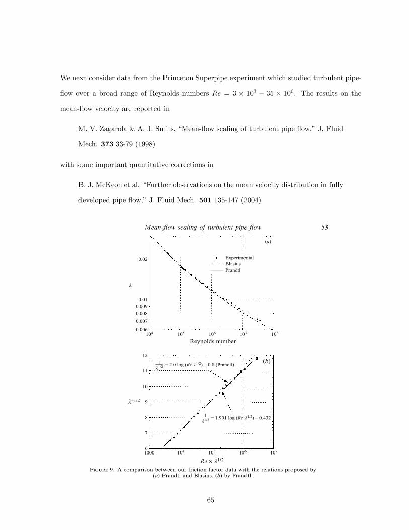
We next consider data from the Princeton Superpipe experiment which studied turbulent pipe-

flow over a broad range of Reynolds numbers Re = 3 " 103 ! 35 " 106. The results on the

mean-flow velocity are reported in

M. V. Zagarola & A. J. Smits, “Mean-flow scaling of turbulent pipe flow,” J. Fluid

Mech. 373 33-79 (1998)

with some important quantitative corrections in

B. J. McKeon et al. “Further observations on the mean velocity distribution in fully

developed pipe flow,” J. Fluid Mech. 501 135-147 (2004)

Mean-flow scaling of turbulent pipe flow 53

0.02

0.010.009

0.008

0.007

0.006104 105 106 107 108

ExperimentalBlasiusPrandtl

(a)

k

Reynolds number

12

11

10

9

8

7

6

k–1/2

(b)

1000 104 105 106 107

1k1/2 = 2.0 log (Re k1/2) – 0.8 (Prandtl)

1k1/2 = 1.901 log (Re k1/2) – 0.432

Re ! k1/2

F!"#$% 9. A comparison between our friction factor data with the relations proposed by(a) Prandtl and Blasius, (b) by Prandtl.

that the constants chosen by Prandtl do not accurately represent our data. A least-squares approximation (no weighting) was used with our data to determine new valuesfor the coe!cient in (25). When all Reynolds numbers are used in the analysis (Case1 in table 3), the new values for the constants are 1!901 and "0!432. The agreementbetween this new curve and the data is satisfactory (see figure 9b), but more accuraterelationships can be found as follows.

As discussed earlier, it seems reasonable to disregard the data below # 100$10!

when determining the coe!cients in (25). Also, there may be a slight roughness e"ectat the very highest Reynolds number. Therefore, the coe!cients in (25) weredetermined using 98$10!%Re% 30$10" (Case 4 in table 3). For comparison withthis Reynolds number range, the analysis was repeated for the di"erent ranges givenin table 3, where R

cis the correlation coe!cient. The results from a least-squares

approximation of Nikuradse’s friction factor data are also given for two di"erentranges of Reynolds numbers. The coe!cients found from Nikuradse’s data for3!1$10!&Re& 3!2$10" are the same as those determined by Prandtl. The values of

65

The first figure (above) shows the results on the friction factor $ = 8(u!/um)2, which are well-

described by the Prandtl logarithmic friction law (with modified coe!cient). The next figure

(below) shows the velocity profiles in inner scaling for 13 di"erent Reynolds numbers.


40

35

30

25

20

15

10

5

0100 101 102 103 104 105 106

y+

U +

U + = 10.41 ln y+ + 5.2

Re = 35 ! 106

10 ! 106

3.1 ! 106

1.0 ! 106

310 ! 106

98 ! 103

31 ! 103

F!"#$% 14. A comparison of the velocity profiles normalized using inner scaling variables for 13di!erent Reynolds numbers between 31!10! and 35!10".

then the near-wall limit of the log law (Mi) should become apparent. If the wall-normal

positions are scaled by outer layer variables, then the core limit of the log law (Mo)

should become apparent.The value of ! was calculated using the value of ! determined from the friction

factor and centreline velocity data (!" 0#436). Data for y!R$ 0#01 were neglected inthis analysis due to the large uncertainty in position and the data at the very highestReynolds number were neglected due to the possibility of roughness e!ects (see figure8). To determine the inner limit, the ! data at each y+ location were averaged. Datafor y!R%M

owere neglected to prevent data in the core region, where !%B, from

increasing the average at a given y+. To determine the outer limit, the ! data at eachy!R location were averaged. Data for y+$M

iwere neglected to prevent data in the

near-wall region, where !$B, from reducing the average at a given y!R. The limitswere adjusted until a consistent value of ! was obtained for some intermediate regiongiven by M

i"!u# $ y$M

oR.

The results are shown in figure 15(a, b). The error bars shown correspond to thestandard error (95% confidence interval) at a given position. These error bars areconsiderably smaller than the uncertainty in B for a single Reynolds number (&0#12)(see figure 8). The large uncertainty in figure 8 is due primarily to the uncertainty in u#

which has a fixed value at a given Reynolds number. When an average is taken overmultiple Reynolds numbers, the random error in u# tends to cancel providing us witha more accurate method to determine B. The values of ! shown in figure 15(a, b) areaverages for data at six to seventeen Reynolds numbers. Inspection of figures 15(a) and15(b) shows that for 600"!u# $ y$ 0#07R (600$ y+$ 0#07R+), ! has a constant valueof 6#15 in both figures.

Our proposed log-law limits are more restrictive than the commonly accepted limitsof 50"!u# $ y$ 0#15R but are consistent with Millikan’s proposal in that a logarithmicoverlap region can only exist for "!u#i yiR or 1i y+iR+. These limits are also

We next show the results for

# # u/u! ! 1$ ln y+

with the value of % inferred from the friction law, % = 0.436. This quantity should equal the

constant B in the logarithmic region. A plateau is observed in the range

600 < y+ < 0.07R+,

smaller than was previously expected.

66

62 M. V. Zagarola and A. J. Smits

7.0

6.5

6.0

5.5

5.0

(a)

101 102 103 104 105

y+

W

B = 6.15

7.0

6.5

6.0

5.5

5.00.01 0.1 1

B = 6.15

y/R

(b)

F!"#$% 15. The di!erence between the velocity profile and the log law as a function of wall-normalposition for !! 0"436. The value of ! was averaged over multiple Reynolds numbers. In (a) the wall-normal positions are normalized using inner scaling variables, and in (b) outer scaling variables.

similar to the ones determined by George et al. (1997) (300# y+# 0"1R+) from asimplified turbulence model. Accepting our proposed limits, a log law cannot exist forR+# 600!0"07! 9$10! which corresponds to a pipe Reynolds number of 400$10!.It is doubtful that other experiments could have defined these limits since to observea log law over an order of magnitude in y+ requires data at a Reynolds number of5$10" which has only been obtained here and in the experiment by Dickinson (1975).

Critics of the log law often point to the Reynolds number dependence of the peakin the Reynolds shear stress, which may occur in the log region, as evidence against theexistence of a log region. This criticism is based on the belief that if the log region istruly an inertial region then the turbulence statistics must be independent of viscouse!ects. We argue that the limits we propose resolve this apparent contradiction. Anequation for the Reynolds shear stress in the log region can be derived from thestreamwise momentum equation as

%u&+! 1%y+

R+%

1

!y+, (41)

where %u&+ is the Reynolds shear stress normalized by u". Equation (41) can be usedto show that the peak in %u&+ occurs at

y+p! 01!R+1#/$. (42)

If a log law is not observed until R+& 9$10!, then the location of the peak isinconsequential since %u&+& 1 and viscous e!ects are negligible. This is not the caseif we use the conventional limits for the log law since a log law would then exist atR+& 50!0"15& 330 and

%u&+! 1%0 4

!R+1#/$! 0"83 (43)

if we let !! 0"41. The proposed log-law limits are consistent with the streamwise

The next figures show that no choice of % succeeds to extend the plateau to y+ < 600 and that

the region is better fit by a power-law

u/u! = 8.70(y+)0.137.

The outer range of the power-law is found to be

y+ = min{500, 0.15R+}

so that the range does not grow for Re! > 3300.

67


D! = 0 (! = 0.436)D! = + 0.002D! = + 0.004D! = – 0.002D! = – 0.004

101 102 103 104 105

y+

7.0

6.5

6.0

5.5

5.0

B = 6.15

W

F!"#$% 16. The di!erence between the velocity profile and the log law as a function of wall-normalposition for di!erent values of !. The value of ! was averaged over multiple Reynolds numbers.

30

25

20

15

10

5

0100 101 102 103 104 105

y+

U+

U+ = y+

U+ = 8.70(y+)0.137 U+ =1

0.436 ln y+ + 6.15

F!"#$% 17. A linear–log plot of the velocity profile data within 0!07R+ of the wall normalizedusing inner scaling variables for 26 di!erent Reynolds numbers from 31"10! to 35"10".

momentum equation while the previously accepted limits appear to create acontradiction between the equations of motion and the overlap argument used toderive the log law.

The new log-law limits were used to determine B for each Reynolds number. Theresults are shown in figure 8 which is described in §5. The additive constant has anaverage value of 6!15 with a standard error of #0!02 when the highest Reynoldsnumber is neglected. No Reynolds number dependence is apparent except at thehighest Reynolds number and, as pointed out in §5, this may be caused by roughness.

So far we have assumed that !$ 0!436. In figure 16 we show ! for !$ 0!436#0!002and #0!004. The data for !$ 0!436 and !$ 0!438 form a horizontal line for y+% 600.For !$ 0!438 the nominal value of B is 6!23. For the other values of !, ! has either

68


20

10101 102 103 104

y+

U+ U+ = 8.70(y+)0.137

F!"#$% 19. A log–log plot of the velocity profile data within 0!07R+ of the all normalized usinginner scaling variables for 26 di!erent Reynolds numbers from 31"10! to 35"10".

We believe that this region, which is closer to the wall than the log region and furtherfrom the wall than the linear region, is better described by a power law than a log law(Zagarola & Smits 1997). The power law is shown in figure 17. The local value of ! canbe evaluated from the slope of the power law using

!# 0y+dU+

dy+ 1!#. (45)

The value of ! varies from 0!49 to 0!36 for 50$ y+$ 500 which is consistent with thevariation observed by many previous investigators (Hinze 1964), and helps explain whyprevious investigators have noted a Reynolds number dependence of the log-lawconstants.

Finding the empirical constants and the limits of a power law are more di"cult thanfor the log law since neither of the constants is readily determined from the frictionfactor data. The inner limit of the power law should scale on inner layer variables, butthe outer limit may scale on inner or outer layer variables depending on whether theReynolds number is large enough for a logarithmic overlap region to exist. Frominspection of figure 17, the inner limit of the power law appears to be at y+% 50 or 60.At Reynolds numbers su"ciently large for a log law to exist (R+% 9"10!), we mayexpect that the outer limit of the power law region is equivalent to the inner limit ofthe log law (y+% 600). At lower Reynolds numbers, we expect viscous e!ects and thepower law scaling to extend beyond where the outer limit of the log law is located(y+% 0!07R+). We can take y+# 0!15R+ as a first approximation since it is theconventional outer limit of the log law.

The empirical constants in the power law were determined using a least-squaresapproximation for the region given by 60$ y+$ 500 or 0!15R+. The data for 500$y+$ 600 are inconsistent with the power law scaling, and we believe that this regionis a transition region between the power law and log law. In figure 19 we plot the U+

data in log–log coordinates in order to emphasize the power law dependence. Thepower law is given by

U+# 8!70(y+)$!#!%. (46)

The U+ data are within &0!72% (# 2"standard deviation) of (46) for 60$ y+$ 500


104

103

102

101

102 103 104 105

R+

y+ @

out

er li

mit

of p

ower

law y+ = 500

y+ = 0.15R+

F!"#$% 20. The outer limit of the power law region as a function of Reynolds number.

or 0!15R+ which is commensurate with the uncertainty in U+ ("0!57%). Themultiplicative constant and the exponent in (46) are very close to the values (8!74,1!7# 0!143) that Prandtl derived (see Durand 1943) from the Blasius friction factorrelation (equation (32)) using the assumption U! # 0!8U

CL, and which Nikuradse

(1932) showed were in good agreement with his low Reynolds number data.In figure 20, we show the outer limit of the power law as a function of R+. The outer

limit was determined as the point where the uncertainty intervals of the U+ data nolonger overlap (46). The outer limit appears to depend on Reynolds number for R+$6%10!, and above this value, it appears to be independent of Reynolds number andconstant at approximately y+& 500. For R+$ 2!7%10!, the outer limit is in reasonableagreement with y+# 0!15R+. For 2!7%10!$R+$ 5%10!, the power law appears toextend considerably further into the outer region (y& 0!3R to 0!6R) than for the otherReynolds numbers. We believe that this anomaly occurs because the slope of thevelocity profile at the outer limit of the power law, which depends on R+, coincides withthe slope near the inner limit of the outer region at these Reynolds numbers. We do notbelieve that the extension of the power law this far from the wall is indicative of aviscous dependence.

8. A new scaling argument for the inner region

The existence of a power law implies that viscosity is still an important parameter fory+$ 500. The viscous dependence suggests that this region is part of the inner region,but since the Reynolds number must be quite large for this region to exist, it could alsobe an overlap region exhibiting incomplete similarity (Zagarola & Smits 1997). Thelowest Reynolds number where the power law exists is Re& 13%10! (R+& 400). Theexistence of an overlap region at this Reynolds number is supported by theinvestigation by Patel & Head (1969) in which they observed an overlap region forRe' 10!. They concluded that the overlap region was logarithmic, but it is doubtfulthat the scaling could be determined at such low Reynolds numbers.

It could also be argued that at su!ciently high Reynolds numbers the power lawbecomes the log law. This scenario is consistent with Prandtl’s speculation (see Durand

69

Finally, we present some results of Zagarola & Smits (1998) on outer scaling. They found that

(uc! um)/u! $ const. as Re$%, consistent with standard theory. On the other hand, better

collapse in outer scaling was obtained by using uc ! um as the velocity scale rather than the

conventional quantity u!.


5.0

4.8

4.6

4.4

4.2

4.0104 105 106 107 108

Reynolds number

(UC

L –

U)/

u s

F!"#$% 22. The di!erence between the average and centreline velocityas a function of Reynolds number.

Barenblatt (1993). Both proposals presume a smooth or gradual variation of thescaling in the overlap region. The proposal by George et al. presumes a smoothvariation of y+dU+!dy+ with y+. The proposal by Barenblatt presumes a smoothvariation of C

!and ! with Reynolds numbers. The variation of y+dU+!dy+ at four

di!erent Reynolds number is shown in figure 21. These proposals clearly di!er in spiritfrom the proposal given here. Despite the abrupt change in scaling, we note that theentire overlap region in our model is still described only in terms of classic inner andouter scales. The functional dependence is observed to change, but the power-law andlog-law regions should not be thought of as two separate overlap regions because theyshare the same scaling variables.

For our overlap proposal to be valid, uomust be proportional to u" at high Reynolds

number. From our analysis, it appears that a reasonable candidate for uo

is UCL

!U! ,which is a true outer velocity scale, in contrast to u", which is a velocity scale associatedwith the near-wall region which is ‘ impressed’ on the outer region. Figure 22 shows thevariation of (U

CL!U! )!u" with Reynolds number. At Reynolds numbers less than

" 300#10", uo!u" is a function of Reynolds number, but at high Reynolds numbers,

uo!u" is independent of Reynolds number (i.e. u

o!u" $ constant). For Reynolds

numbers greater than 300#10", the error bounds for all data overlap a horizontal lineat (U

CL!U! )!u" $ 4%34. If U

CL!U! is the correct outer velocity scale, then it should

collapse the velocity profiles in the outer region for di!erent Reynolds numbers ontoa single curve. A comparison between the velocity profiles in the outer region scaled byU

CL!U! and u" is given in §9.

9. Velocity profile results : Outer scaling

In figure 23(a, b) we plot the velocity profiles scaled by u" and UCL

!U! for sevendi!erent Reynolds numbers between 31#10" and 35#10#. When the velocity profilesare scaled by u", the profiles do not collapse onto a single curve. The poor collapse isparticularly evident for 0%07& y!R& 0%30 which is part of the overlap or core regiondepending on the Reynolds number. When using U

CL!U! to scale the profiles (figure

23b), the collapse of the profiles is much improved for y!R' 0%10. For both scalings,

70


15

10

5

0

(a)

(b)

31 ! 103

98 ! 103

310 ! 103

1.0 ! 106

3.1 ! 106

10 ! 106

35 ! 106

Re

(UC

L –

U)/

us

3

2

1

00.01 0.1 1

y/R

(UC

L –

U)/

(UC

L –

U)

F!"#$% 23. A comparison between the velocity profiles normalized by (a) u! and (b) UCL

!U! forReynolds numbers between 31"10! and 35"10".

the collapse in the overlap region is not very satisfactory. For low Reynolds numbers,this behaviour should be expected because an overlap region which is independent ofReynolds number (log law) does not exist for Re# 400"10!.

The di!erence between the velocity scales is more evident at low Reynolds numberssince at high Reynolds numbers the scales are proportional. Therefore, in figure24(a, b) we plot the velocity profiles normalized by u! and U

CL!U! , respectively, for all

Reynolds numbers investigated between 31"10! and 540"10!. A comparison betweenthe figures 24(a) and 24(b) indicates that the data scaled by U

CL!U! are in much better

agreement for y!R$ 0%07 than the data scaled by u!. The only profile that is not in

We now consider more results from the Superpipe experiments in

M. V. Zagarola, A. E. Perry & A. J. Smits, “Log laws or power laws: the scaling in

the overlap region,” Phys. Fluids 9 2094-2100 (1997)

71

which tested the Barenblatt-Chorin theory. As seen from the first figure, the BC theory (with

constants fit from the old data of Nikuradze) has a decreasing less good fit at increasing Reynolds

numbers. Fitting a power law to their data over the range 40 < y+ < 0.85R+, the authors

found a best fit as u/u! = Cy&+ with

" = 1.085ln Re + 6.535

(ln Re)2

C = 0.1053(lnRe) + 0.3055.

These power-laws gave a reasonable fit to the data, but with larger fractional di"erences than

a fit by a log-law, especially at higher Reynolds numbers.

shown to be logarithmic.11 For incomplete similarity, the ve-

locity gradient depends on one or both length scales, and the

scaling of the velocity profile has been shown to be a power

law using a number of different arguments.2,9,12

II. RESULTS AND DISCUSSION

In Fig. 1, we plot 13 mean velocity profiles measured in

the SuperPipe facility normalized by inner scaling variables.

From an analysis of all 26 velocity profiles, Zagarola and

Smits13 concluded that for y!"0.1R! (y"0.1R), the meanvelocity profile is independent of Reynolds number, or

equivalently, the outer length scale R . In Fig. 2, all 26 ve-

locity profiles are plotted for y!"0.1R! only, and no Rey-

nolds number dependence is evident in this figure. Zagarola

and Smits also proposed that the mean velocity profile con-

sists of two distinct regions: a power-law region for

50"y!"500 or 0.1R!, and a log-law region for

500"y!"0.1R!. The outer limit of the power law is given

by y!!0.1R! if R!"5#103, and by y!!500 if

R!$5#103. The power law is given by

U!%8.70"y!#0.137. "7#

Equation "7# should not be confused with the 1/7 power-lawrelation proposed by Prandtl7 which is an empirical represen-

tation of the entire velocity profile at low Reynolds numbers

(R!"2.4#103). Equation "7# was derived from an overlap

FIG. 5. Comparison between the mean velocity profiles and Eq. "14# for 4different Reynolds numbers between 31#103 and 35#106. The error barsrepresent an uncertainty in U! of &0.57%.

FIG. 6. Plot of the multiplicative constant in the power law given by Eq.

"10# for 26 different Reynolds numbers between 31#103 and 35#106.

FIG. 7. Plot of the exponent in the power law given by Eq. "10# for 26different Reynolds numbers between 31#103 and 35#106.


2096 Phys. Fluids, Vol. 9, No. 7, July 1997 Zagarola, Perry, and Smits

Downloaded¬14¬Apr¬2008¬to¬128.220.254.4.¬Redistribution¬subject¬to¬AIP¬license¬or¬copyright;¬see¬http://pof.aip.org/pof/copyright.jsp

72



















U!%8.70"y!#0.137. "7#





























U!%8.70"y!#0.137. "7#











73



















U!%8.70"y!#0.137. "7#











Barenblatt & Chorin in

G. I. Barenblatt & A. J. Chorin, “Scaling of the intermediate region in wall-bounded

turbulence: the power-law,” Phys. Fluids 10 1043-1044 (1998)

have imputed the disagreement with the Superpipe data at the higher Reynolds numbders to

the e"ects of roughness, which should become more important as Re increases. The issue of

roughness has been addressed by

M. A. Shockling, J. J. Allen & A. J. Smits, “Roughness e"ects in turbulent pipe

flow,” J. Fluid Mech. 564 267-285 (2006)

By performing new experiments with increased k+, the e"ects of roughness were systematically

studied.

74

272 M. A. Shockling, J. J. Allen and A. J. Smits

Tomotor

Pumping section Heatexchanger

Return leg

Flow

FlowDiffusersection

Test pipe

Primary testsection

Test leg Flow conditioningsection

34 m

1.5 m

Figure 1. Princeton/ONR Superpipe facility.

0.20

(a) (b)

0.15

0.10

0.05

0 0.05 0.10x (mm)

z (m

m)

0.15 0.20 0.25

3.0

2.5

2.0

1.5

1.0

0.5

0–0.5 0

Amplitude (µm)P

DF

(am

plit

ude)

0.5 1.0

Figure 2. (a) Two-dimensional surface plot of the original Superpipe. Area shown is about0.2mm ! 0.25 mm, and the amplitudes are in µm. (b) Probability density function of surfaceelevation.

The test pipe is located inside the closed-return pressure vessel, and it is approx-imately 0.129 m in diameter and 25.9 m in length, so that the length-to-diameter ratioexceeds 200. Two test ports are available at 160D and 196D downstream of thecontraction, and all profiles were measured at the downstream location during theseexperiments. The pipe was constructed using 5 in. (129 mm) ID, 1/2 in. (12.7mm)thick drawn aluminum tube. Six sections of tube, approximately 4.6 m in length, wereconnected and the centreline axis was aligned to within ±1.25 mm over a distanceof 30 m using the alignment procedure described by Zagarola (1996). Since the pipesections were connected during honing, the maximum step measured at each jointduring installation was about ±0.025 mm over the entire length of the pipe, negligiblysmall according to Zagarola (1996).

The pipe surface roughness was designed to be geometrically similar to the surfaceused by Zagarola & Smits (1998) and McKeon et al. (2004) while preserving a lowkrms/D. A machined surface roughness is typically described using the roughness andr.m.s. amplitudes, defined respectively as Ra =

! L

0 |y/L| dx, and Rq =(! L

0 (y/L)2 dx)1/2,where y is the surface height deviation from the mean level. For the original Superpipesurface, comparator plates indicated that Ra " 0.15 µm. To better define the geometryof the surface roughness, a non-interfering, two-dimensional optical measurement wasmade of the original Superpipe surface, as shown in figure 2. From this image, it is

Roughness e!ects in turbulent pipe flow 273

1.0

(a)

0.5

0 0.5x (mm)

z (m

m)

1.0

0.16

0.12

0.08

0.04

0–5 0

Amplitude (µm)

PD

F (

ampl

itud

e)

5 10

(b)

Figure 3. (a) Two-dimensional surface plot of the new rough pipe. Area shown is about0.8mm ! 1.2 mm, and the amplitudes are in µm. (b) Probability density function of surfaceelevation.

clear that a particular wavelength has been imparted to the surface as a result of thehoning process. However, it can also be seen that the probability density function ofthe surface elevation closely resembles a normal distribution, with a skewness of only"0.31, and a flatness of 3.6. The data give Ra = 0.116 µm and Rq =0.15 µm, in goodagreement with the original comparator plate measurements.

One other useful measure that is relevant to the pipe surface design is the highspot count (HSC), which is the number of peaks per unit length that exceed a certainthreshold. Using a threshold value for the peak counts equal to Rq results in a meanwavelength, defined as !HSC = 1/HSC of 0.01 mm. Therefore the ratio of roughnessheight to wavelength was very small in the original Superpipe experiments (#1/62),and raises the question as to whether traditional concepts such as form drag behinddiscrete objects can be used to describe the flow field over such a surface.

The new rough pipe was designed using the Colebrook roughness function so thatthe flow was expected to be smooth up to ReD # 500 ! 103, and fully rough forReD > 8 ! 106. A surface with an equivalent sandgrain roughness value of ks = 7.6 µmappeared to satisfy these requirements. Using ks # 3krms , as suggested by Zagarola &Smits (1998), gives krms = 2.5 µm, and the new pipe was honed to obtain this roughnessand an appropriately scaled !HSC.

Figure 3 shows a two-dimensional plot of the surface elevation, generated using anoptical scanner of the new surface. For this surface, Rq =2.5 µm and Ra =1.92 µm.The surface skewness was Sk = 0.31 and the flatness was 3.43. Again, these resultssuggest that the roughness distribution is close to being Gaussian. Using a thresholdvalue for the peak counts equal to Rq gives !HSC = 90 µm, and an amplitude-to-wavelength ratio of # 1/37. Although the rough surface is not geometrically identicalto the original Superpipe smooth surface, it is expected that the roughness scaling forthis surface will reflect closely the behaviour of the smooth Superpipe at equivalentk+

s conditions since both surfaces show nearly Gaussian roughness distributions.

5. Measurement techniquesMean velocity profiles were taken 196D downstream of the test pipe inlet. A

removable oval shaped plug, 100 mm ! 50 mm wide was inserted into the test pipe,

75

A first result is shown for the friction factor $ = 8(u!/um)2, which shows no e"ects of

roughness for Re < 106, in agreement with original claims of Zagarola & Smits. The friction

coe!cient is non-monotonic in the Reynolds number, showing a “belly” qualitatively similar to

that seen in the old data of Nikuradze.


105 107106

0.008

0.010

0.012

0.014

0.016

0.018

0.020

0.022

ReD

!

McKeon SmoothColebrook RoughNikuradse, R/ks = 507Rough pipe

Figure 6. Friction factor ! for the present surface, compared with the rough-all relationsof Colebrook (1939) for the same ks , the smooth-wall relation of McKeon et al. (2005)(equation (2.4)), and the results for the smallest sandgrain roughness used by Nikuradse(1933).

105 106 1070.010

0.012

0.014

0.016

0.018

0.020

ReD

!

CorrectedUncorrected

Figure 7. Friction factor ! for the present surface, comparing the data using corrections asdescribed in § 6 and the data without any corrections.

friction factor begins to depart from the smooth curve, reaching a local minimum of!! 0.0106 in the region 3.1 " 106 <ReD < 4.0 " 106. The friction factor then rises to aconstant value of != 0.0108 for ReD > 10 " 106. The equivalent sandgrain roughnessfor this surface, defined by the friction factor in the fully rough regime, is ks = 7.4 µm= 3krms , in good agreement with Zagarola & Smits’s (1998) estimate ks ! 3krms for thesmooth pipe data.

Figure 7 shows a comparison of the friction factor as calculated with the prescribedPitot and static corrections to the friction factor without any corrections applied (for

76

Shockling et al. have also studied the downward velocity profile shift with roughness, which has

been observed in previous studies as well. There are no e"ects of roughness in the new rough

pipe for k+s < 3.5, again bolstering their previous claims about the lack of roughness e"ects in

the smooth-pipe experiment.


100 101 102

1

2

3

4

5

6

7

8

9

10

ks+

B!

Rough pipeNikuradse (1933)B! = 5.5 + 5.75 log(k+)B! = 8.48

Figure 16. The velocity profile shift according to Nikuradse’s roughness scaling, showingsmooth, transitional, and fully rough regimes.

10–2 10–1 1000

5

10

15

! = y/R ! = y/R

(UC

L –

U)/

U"

0.2 0.4 0.6 0.8 1.00

5

10

15

Figure 17. Outer scaling for 349 ! 103 ! ReD ! 21.2 ! 106. Solid line: "(1/0.421) ln ! + 1.20.

slightly lower roughness Reynolds number, k+s , which may be an e!ect of the random

variation in surface elevation; honed roughness has a nearly Gaussian roughnessdistribution, whereas the roughness elements used by Ligrani & Mo!at (1986) andNikuradse (1933) had an extremely narrow bandwidth and would not necessarilypossess a Gaussian distribution.

7.3. Velocity profiles: outer scaling

Figure 17 shows a collection of velocity profiles for Re " 349 ! 103 scaled on outerflow coordinates, y/R. It appears that the velocity profiles collapse well, as expectedaccording to Townsend’s outer flow similarity hypothesis for rough-wall flows. Thecollapse in outer layer coordinates is comparable to that demonstrated by Zagarola& Smits (1998) for the smooth Superpipe data and by Flack et al. (2005) in theirrough-wall boundary layer studies.

77

Finally, Shockling et al. have verified Townsend’s “outer layer similarity hypothesis,” which

states that there should be no e"ect of roughness in the outer layer, except for the change

in friction velocity uk. The authors observe excellent scaling of the velocity profiles in outer

scaling for the smooth and rough pipe experiments.


100 101 102

1

2

3

4

5

6

7

8

9

10

ks+

B!

Rough pipeNikuradse (1933)B! = 5.5 + 5.75 log(k+)B! = 8.48

Figure 16. The velocity profile shift according to Nikuradse’s roughness scaling, showingsmooth, transitional, and fully rough regimes.

10–2 10–1 1000

5

10

15

! = y/R ! = y/R

(UC

L –

U)/U

"

0.2 0.4 0.6 0.8 1.00

5

10

15

Figure 17. Outer scaling for 349 ! 103 ! ReD ! 21.2 ! 106. Solid line: "(1/0.421) ln ! + 1.20.

slightly lower roughness Reynolds number, k+s , which may be an e!ect of the random

variation in surface elevation; honed roughness has a nearly Gaussian roughnessdistribution, whereas the roughness elements used by Ligrani & Mo!at (1986) andNikuradse (1933) had an extremely narrow bandwidth and would not necessarilypossess a Gaussian distribution.

7.3. Velocity profiles: outer scaling

Figure 17 shows a collection of velocity profiles for Re " 349 ! 103 scaled on outerflow coordinates, y/R. It appears that the velocity profiles collapse well, as expectedaccording to Townsend’s outer flow similarity hypothesis for rough-wall flows. Thecollapse in outer layer coordinates is comparable to that demonstrated by Zagarola& Smits (1998) for the smooth Superpipe data and by Flack et al. (2005) in theirrough-wall boundary layer studies.

78

fig. 38 insensitivity of wake strength at high (g) numerical and...

Documents