feynman motives of banana graphsmarcolli/bananamot.pdfresults in a change of sign to one of the...
TRANSCRIPT
FEYNMAN MOTIVES OF BANANA GRAPHS
PAOLO ALUFFI AND MATILDE MARCOLLI
Abstract. We consider the infinite family of Feynman graphs known as the “bananagraphs” and compute explicitly the classes of the corresponding graph hypersurfacesin the Grothendieck ring of varieties as well as their Chern–Schwartz–MacPhersonclasses, using the classical Cremona transformation and the dual graph, and a blowupformula for characteristic classes. We outline the interesting similarities between theseoperations and we give formulae for cones obtained by simple operations on graphs.We formulate a positivity conjecture for characteristic classes of graph hypersurfacesand discuss briefly the effect of passing to noncommutative spacetime.
1. Introduction
Since the extensive study of [15] revealed the systematic appearance of multiple zetavalues as the result of Feynman diagram computations in perturbative quantum field the-ory, the question of finding a direct relation between Feynman diagrams and periods ofmotives has become a rich field of investigation. The formulation of Feynman integralsthat seems most suitable for an algebro-geometric approach is the one involving Schwingerand Feynman parameters, as in that form the integral acquires directly an interpretationas a period of an algebraic variety, namely the complement of a hypersurface in a projectivespace constructed out of the combinatorial information of a graph. These graph hyper-surfaces and the corresponding periods have been investigated in the algebro-geometricperspective in the recent work of Bloch–Esnault–Kreimer ([10], [11]) and more recently,from the point of view of Hodge theory, in [12] and [26]. In particular, the question ofwhether only motives of mixed Tate type would arise in the quantum field theory contextis still unsolved. Despite the general result of [8], which shows that the graph hypersur-faces are general enough from the motivic point of view to generate the Grothendieck ringof varieties, the particular results of [15] and [11] point to the fact that, even though thevarieties themselves are very general, the part of the cohomology that supports the periodof interest to quantum field theory might still be of the mixed Tate form.
One complication involved in the algebro-geometric computations with graph hyper-surfaces is the fact that these are typically singular, with a singular locus of small codi-mension. It becomes then an interesting question in itself to estimate how singular thegraph hypersurfaces are, across certain families of Feynman graphs (the half open laddergraphs, the wheels with spokes, the banana graphs etc.). Since the main goal is to de-scribe what happens at the motivic level, one wants to have invariants that detect howsingular the hypersurface is and that are also somehow adapted to its decomposition inthe Grothendieck ring of motives. In this paper we concentrate on a particular exampleand illustrate some general methods for computing such invariants based on the theory ofcharacteristic classes of singular varieties.
Part of the purpose of the present paper is to familiarize physicists working in pertur-bative quantum field theory with some techniques of algebraic geometry that are usefulin the analysis of graph hypersurfaces. Thus, we try as mush as possible to spell outeverything in detail and recall the necessary background.
1

2 ALUFFI AND MARCOLLI
In §1, we begin by recalling the general form of the parametric Feynman integrals fora scalar field theory and the construction of the associated projective graph hypersurface.We recall the relation between the graph hypersurface of a planar graph and that ofthe dual graph via the standard Cremona transformation. We then present the specificexample of the infinite family of “banana graphs”. We formulate a positivity conjecturefor the characteristic classes of graph hypersurfaces.
For the convenience of the reader, we recall in §2 some general facts and results, bothabout the Grothendieck ring of varieties and motives, and about the theory of characteristicclasses of singular algebraic varieties. We outline the similarities and differences betweenthese constructions.
In §3 we give the explicit computation of the classes in the Grothendieck ring of thehypersurfaces of the banana graphs. We conclude with a general remark on the relationbetween the class of the hypersurface of a planar graph and that of a dual graph.
In §4 we obtain an explicit formula for the Chern–Schwartz–MacPherson classes ofthe hypersurfaces of the banana graphs. We first prove a general pullback formula forthese classes, which is necessary in order to compute the contribution to the CSM class ofthe complement of the algebraic simplex in the graph hypersurface. The formula is thenobtained by assembling the contribution of the intersection with the algebraic simplex andof its complement via inclusion–exclusion, as in the case of the classes in the Grothendieckring.
We give then, in §5, a formula for the CSM classes of cones on hypersurfaces anduse them to obtain formulae for graph hypersurfaces obtained from known one by simpleoperations on the graphs, such as doubling or splitting an edge, and attaching single-edgeloops or trees to vertices.
Finally, in §6, we look at the deformations of ordinary φ4 theory to a noncommutativespacetime given by a Moyal space. We look at the ribbon graphs that correspond tothe original banana graphs in this noncommutative quantum field theory. We explainthe relation between the graph hypersurfaces of the noncommutative theory and of theoriginal commutative one. We show by an explicit computation of CSM classes that innoncommutative QFT the positivity conjecture fails for non-planar ribbon graphs.
Acknowledgment. The first author is partially supported by NSA grant H98230-07-1-0024. The second author is partially supported by NSF grant DMS-0651925. We thankthe Max–Planck–Institute and Florida State University, where part of this work was done.We also thank Abhijnan Rej for exchanges of numerical computations of CSM classes ofgraph hypersurfaces.
1.1. Parametric Feynman integrals. We briefly recall some well known facts (cf. §6-2-3of [23], §18 of [9], and §6 of [27]) about the parametric form of Feynman integrals.
Given a scalar field theory with Lagrangian written in Euclidean signature as
(1.1) L(φ) =1
2(∂φ)2 +
m2
2φ2 + Lint(φ),
where the interaction part is a polynomial function of φ, a one-particle-irreducible (1PI)Feynman graph of the theory is a connected graph Γ which cannot be disconnected byremoving a single edge, and with the following properties. All vertices in V (Γ) havevalence equal to the degree of one of the monomials in the Lagrangian. The set of edgesE(Γ) = Eint(Γ) ∪ Eext(Γ) consists of internal edges having two end vertices and externalones having only one vertex. A Feynman graph without external edges is called a vacuumbubble.
In perturbative quantum field theory, the Feynman integrals associated to the loopnumber expansion of the effective action for a scalar field theory are labeled by the 1PI
BANANA MOTIVES 3
Feynman graphs of the theory, each contributing a corresponding integral of the form
(1.2) U(Γ, p) =Γ(n − D`/2)
(4π)`D/2
∫
[0,1]n
δ(1 −∑
i ti)
ΨΓ(t)D/2VΓ(t, p)n−D`/2dt1 · · · dtn.
Here n = #Eint(Γ) is the number of internal edges of the graph Γ, D ∈ N is the spacetimedimension in which the scalar field theory is considered, and ` = b1(Γ) is the number ofloops in the graph, i.e. the rank of H1(Γ, Z). The function ΨΓ is a polynomial of degree` = b1(Γ). It is given by the Kirchhoff polynomial
(1.3) ΨΓ(t) =∑
T⊂Γ
∏
e/∈E(T )
te,
where the sum is over all the spanning trees T of Γ. The function VΓ(t, p) is a rationalfunction of the form
(1.4) VΓ(t, p) =PΓ(t, p)
ΨΓ(t),
where PΓ is a homogeneous polynomial of degree ` + 1 = b1(Γ) + 1 of the form
(1.5) PΓ(p, t) =∑
C⊂Γ
sC
∏
e∈C
te,
Here the sum is over the cut-sets C ⊂ Γ, i.e. the collections of b1(Γ) + 1 edges that dividethe graph Γ in exactly two connected components Γ1∪Γ2. The coefficient sC is a functionof the external momenta attached to the vertices in either one of the two components
(1.6) sC =
∑
v∈V (Γ1)
Pv
2
=
∑
v∈V (Γ2)
Pv
2
,
where the Pv are defined as
(1.7) Pv =∑
e∈Eext(Γ),t(e)=v
pe,
where the pe are incoming external momenta attached to the external edges of Γ andsatisfying the conservation law
(1.8)∑
e∈Eext(Γ)
pe = 0.
The divergence properties of the integral (1.2) can be estimated in terms of the “superfi-cial degree of divergence”, which is measured by the quantity n−D`/2. The integral (1.2)is called logarithmically divergent when n−D`/2 = 0. The example of the banana graphswe concentrate on below has n = `+ 1, so that we find n−D`/2 = (1−D/2)`+1 < 0 forD > 2 and ` ≥ 2. In this case, we write the integral (1.2) in the form
(1.9) U(Γ, p) =Γ(n − D(n − 1)/2)
(4π)(n−1)D/2
∫
σn
PΓ(p, t)−n+D(n−1)/2 ωn
ΨΓ(t)n(−1+D/2),
where ωn is the volume form and the domain of integration is the topological simplex
(1.10) σn = (t1, . . . , tn) ∈ Rn+ |∑
i
ti = 1.
The 1PI condition on Feynman graphs comes from the fact of considering the pertur-bative expansion of the effective action in quantum field theory, which reduces the combi-natorics of graphs to just those that are connected and 1PI. In terms of the expression ofthe Feynman integral, the 1PI condition is reflected in the fact that only the propagatorsfor internal edges appear. The parametric form we described above therefore depends on

4 ALUFFI AND MARCOLLI
this assumption. However, for the algebro-geometric arguments that constitute the maincontent of this paper, the 1PI condition is not strictly necessary.
1.2. Feynman graphs, varieties, and periods. The graph polynomial ΨΓ(t) of (1.3)also admits a description as determinant
(1.11) ΨΓ(t) = det MΓ(t)
of an ` × `-matrix MΓ(t) associated to the graph ([27], §3 and [9], §18), of the form
(1.12) (MΓ)kr(t) =
n∑
i=1
tiηikηir,
where the n × `-matrix ηik is defined in terms of the edges ei ∈ E(Γ) and a choice of abasis for the first homology group, lk ∈ H1(Γ, Z), with k = 1, . . . , ` = b1(Γ), by setting
(1.13) ηik =
+1 edge ei ∈ loop lk, same orientation
−1 edge ei ∈ loop lk, reverse orientation
0 otherwise,
after choosing an orientation of the edges.Notice how the result is independent of the choice of the orientation of the edges and
of the choice of the basis of H1(Γ, Z). In fact, a change of orientation in a given edgeresults in a change of sign to one of the columns of the matrix ηki, which is compensatedby the change of sign in the corresponding row of the matrix ηir , so that the determinantdet MΓ(t) is unaffected. Similarly, a change in the choice of the basis of H1(Γ, Z) has theeffect of changing MΓ(t) 7→ AMΓ(t)A−1 for some A ∈ GL(`, Z) and the determinant isagain unchanged.
The graph hypersurface XΓ is by definition the zero locus of the Kirchhoff polynomial,
(1.14) XΓ = t = (t1 : . . . : tn) ∈ Pn−1 |ΨΓ(t) = 0.
Since ΨΓ is homogeneous, it defines a hypersurface in projective space.The domain of integration σn defines a cycle in the relative homology Hn−1(P
n−1, Σn),where Σn is the algebraic simplex (the union of the coordinate hyperplanes, see (1.16)below). The Feynman integral (1.2), (1.9) then can be viewed ([11],[10]) as the evaluationof an algebraic cohomology class in Hn−1(Pn−1 r XΓ, Σ r Σ ∩ XΓ) on the cycle definedby σn. In this sense, it can be viewed as the evaluation of a period of the algebraicvariety given by the complement of the graph hypersurface. To understand the natureof this period, one is faced with two main problems. One is eliminating divergences(regularization and renormalization of Feynman integrals), and the other is understandingwhat kind of motives are involved in the part of the hypersurface complement Pn−1 r XΓ
that is involved in the evaluation of the period, hence what kind of transcendental numbersone expects to find in the evaluation of the corresponding Feynman integrals. A detailedanalysis of these problems was carried out in [11]. The examples we concentrate on inthis paper are not especially interesting from the motivic point of view, since they areexpressible in terms of pure Tate motives (cf. [10]), but they provide us with an infinitefamily of graphs for which all computations are completely explicit.
1.3. Dual graphs and Cremona transformation. In the case of planar graphs, thereis an interesting relation between the hypersurface of the graph and the one of the dualgraph. This will be especially useful in the explicit calculation we perform below in thespecial case of the banana graphs. We recall it here in the general case of arbitrary planargraphs.

BANANA MOTIVES 5
The standard Cremona transformation of Pn−1 is the map
(1.15) C : (t1 : · · · : tn) 7→
(
1
t1: · · · :
1
tn
)
.
This is a priori defined away from the algebraic simplex of coordinate axes
(1.16) Σn = (t1 : · · · : tn) ∈ Pn−1 |∏
i
ti = 0 ⊂ Pn−1,
though we see in Lemma 1.2 below that it is well defined also on the general point of Σn,its locus of indeterminacies being only the singularity subscheme of Σn.
Let G(C) denote the closure of the graph of C. Then G(C) is a subvariety of Pn−1×Pn−1
with projections
(1.17) G(C)
π1
π2
??
????
?
Pn−1 C//______ Pn−1
Lemma 1.1. Using coordinates (s1 : · · · : sn) for the target Pn−1, the graph G(C) hasequations
(1.18) t1s1 = t2s2 = · · · = tnsn.
In particular, this describes G(C) as a complete intersection of n − 1 hypersurfaces inPn−1 × Pn−1 with equations tisi = tnsn, for i = 1, . . . , n − 1.
Proof. The equations (1.18) clearly cut out G(C) over the open set U ⊂ Pn where all t-coordinates are nonzero. Since every component of a scheme defined by n−1 equations hascodimension ≤ n−1, it suffices to show that equations (1.18) define a set of codimension >n−1 over the complement of U . Now assume that at least one of the t-coordinates equal 0.Without loss of generality, suppose tn = 0. Intersecting with the locus defined by (1.18)determines the set with equations
t1s1 = · · · = tn−1sn−1 = tn = 0 ,
which has codimension n > n − 1, as promised.
It is not hard to see that the variety G(C) has singularities in codimension 3. It isnonsingular for n = 2, 3, but singular for n ≥ 4.
The open set U as above is the complement of the divisor Σn of (1.16). The inverseimage of Σn in G(C) can be described easily. It consists of the points
((t1 : · · · : tn), (s1 : · · · : sn))
such thati | ti = 0 ∪ j | sj = 0 = 1, . . . , n .
This locus consists of 2N − 2 components of dimension n − 2: one component for eachnonempty proper subset I of 1, . . . , n. The component corresponding to I is the set ofpoints with ti = 0 for i ∈ I and sj = 0 for j 6∈ I .
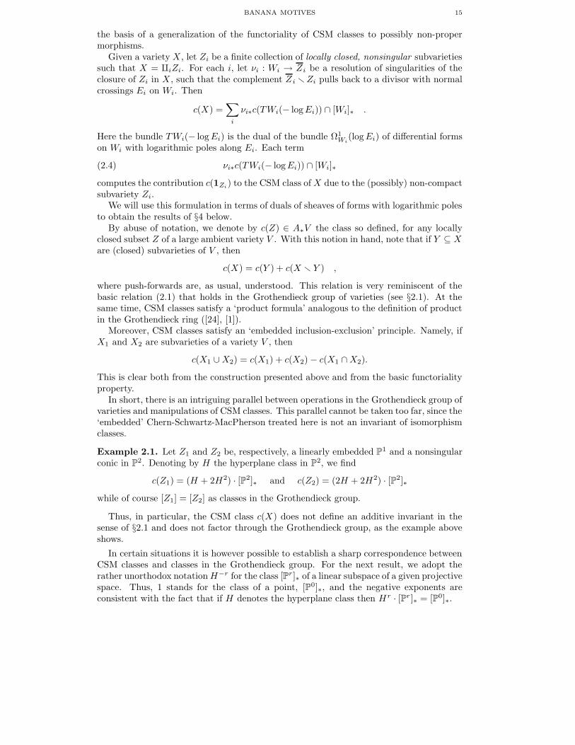
The situation for n = 3 is well represented by the famous picture of Figure 1. Thethree zero-dimensional strata of Σ3 are blown up in G(C) as we climb the diagram fromthe lower left to the top. The proper transforms of the one dimensional strata are blowndown as we descend to the lower right. The horizontal rational map is an isomorphismbetween the complements of the triangles. The inverse image of Σ3 consists of 23 − 2 = 6components, as expected.
Of course the situation is completely symmetric: the algebraic simplex (1.16) may beembedded in the target Pn as well (with equation
∏
i si = 0). One has π−11 (Σn) = π−1
2 (Σn).

6 ALUFFI AND MARCOLLI
Figure 1. The Cremona transformation in the case n = 3.
Let Sn ⊂ Pn−1 be the subscheme defined by the ideal
(1.19) ISn= (t1 · · · tn−1, t1 · · · tn−2tn, . . . , t1t3 · · · tn, t2 · · · tn).
The scheme Sn is the singularity subscheme of the divisor with simple normal crossingsΣn of (1.16), given by the union of the coordinate hyperplanes. We can place Sn in boththe source and target Pn−1. Finally, let L be the hyperplane defined by the equation
(1.20) L = (t1 : · · · : tn) ∈ Pn−1 | t1 + · · · + tn = 0.
We then can make the following observations.
Lemma 1.2. Let C, G(C), Sn, and L be as above.
(1) Sn is the subscheme of indeterminacies of the Cremona transformation C.(2) π1 : G(C) → Pn−1 is the blow-up along Sn.(3) L intersects every component of Sn transversely.(4) Σn cuts out a divisor with simple normal crossings on L.
Proof. (1) Notice that the definition (1.15) of the Cremona transformation, which is apriori defined on the complement of Σn still makes sense on the general point of Σn.Thus, the indeterminacies of the map (1.15) are contained in the singularity locus Sn ofΣn defined by (1.19). It consists in fact of all of Sn since after ‘clearing denominators’,the components of the map defining C given in (1.15) can be rewritten as:
(1.21) (t1 : · · · : tn) 7→ (t2 · · · tn : t1t3 · · · tn : · · · : t1 · · · tn−1) ,
so that one sees that the indeterminacies are precisely those defined by the ideal (1.19).(2) Using (1.21), the map π1 : G(C) → Pn may be identified with the blow-up of Pn
along the subscheme Sn defined by the ideal ISnof (1.19). The generators of this ideal are
the partial derivatives of the equation of the algebraic simplex. Thus, Sn is the singularitysubscheme of Σn. It consists of the union of the closure of the dimension n − 2 strata ofΣn. Again, note that the situation is entirely symmetrical: we can place Sn in the targetPn as well, and view π2 as the blow-up along Sn.
(3) and (4) are immediate from the definitions.

BANANA MOTIVES 7
dual graph
dual graph
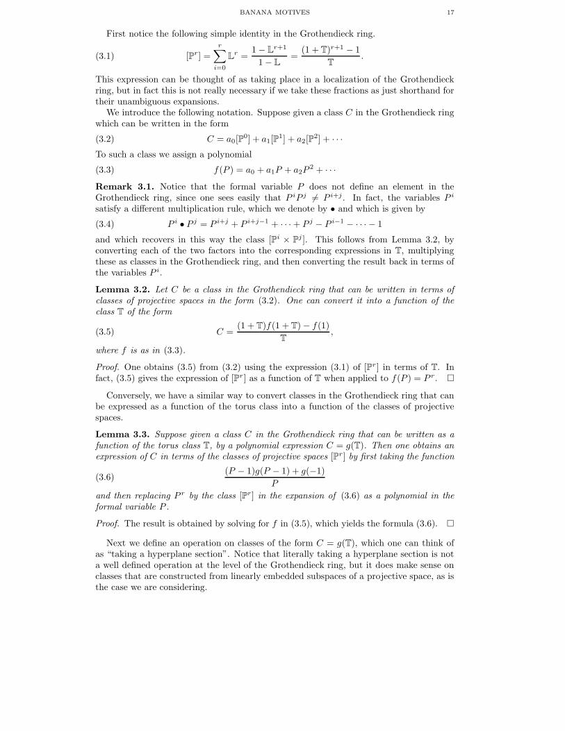
Figure 2. Dual graphs of different planar embeddings of the same graph.
Given a connected planar graph Γ, one defines its dual graph Γ∨ by fixing an embeddingof Γ in R2 ∪ ∞ = S2 and constructing a new graph in S2 that has a vertex in eachcomponent of S2rΓ and one edge connecting two such vertices for each edge of Γ that is inthe common boundary of the two regions containing the vertices. Thus, #E(Γ∨) = #E(Γ)and #V (Γ∨) = b0(S
2 r Γ). The dual graph is in general non-unique, since it depends onthe choice of the embedding of Γ in S2, see e.g. Figure 2.
We recall here a well known result (see e.g. [10], Proposition 8.3), which will be veryuseful in the following.
Lemma 1.3. Suppose given a planar graph Γ with #E(Γ) = n, with dual graph Γ∨. Thenthe graph polynomials satisfy
(1.22) ΨΓ(t1, . . . , tn) = (∏
e∈E(Γ)
te) ΨΓ∨(t−11 , . . . , t−1
n ),
hence the graph hypersurfaces are related by the Cremona transformation C of (1.15),
(1.23) C(XΓ ∩ (Pn−1 r Σn)) = XΓ∨ ∩ (Pn−1 r Σn).
Proof. This follows from the combinatorial identity
ΨΓ(t1, . . . , tn) =∑
T⊂Γ
∏
e/∈E(T ) te
= (∏
e∈E(Γ) te)∑
T⊂Γ
∏
e∈E(T ) t−1e
= (∏
e∈E(Γ) te)∑
T ′⊂Γ∨
∏
e/∈E(T ′) t−1e
= (∏
e∈E(Γ) te)ΨΓ∨(t−11 , . . . , t−1
n ).
The third equality uses the fact that #E(Γ) = #E(Γ∨) and #V (Γ∨) = b0(S2 rΓ), so that
deg ΨΓ + deg ΨΓ∨ = #E(Γ), and the fact that there is a bijection between complementsof spanning tree T in Γ and spanning trees T ′ in Γ∨ obtained by shrinking the edges of Tin Γ and taking the dual graph of the resulting connected graph.
Written in the coordinates (s1 : · · · : sn) of the target Pn−1 of the Cremona transfor-mation, the identity (1.22) gives
ΨΓ(t1, . . . , tn) = (∏
e∈E(Γ∨)
s−1e )ΨΓ∨(s1, . . . , sn)
from which (1.23) follows.
We then have the following simple geometric observation, which follows directly fromLemma 1.2 and Lemma 1.3 above.

8 ALUFFI AND MARCOLLI
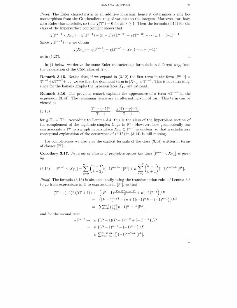
Γ Γ Γ3 4 5
Figure 3. Examples of banana graphs
Corollary 1.4. The graph hypersurface of the dual graph is XΓ∨ = π2(π−11 (XΓ)), with
πi : G(C) → Pn−1, for i = 1, 2, as in (1.17). The Cremona transformation C restricts to a(biregular) isomorphism
(1.24) C : XΓ r Σn → XΓ∨ r Σn.
The map π2 : G(C) → Pn−1 of (1.17) restricts to an isomorphism
(1.25) π2 : π−11 (XΓ r Σn) → XΓ∨ r Σn.
Notice that the formula (1.22) can be used as a source of examples of combinatoriallyinequivalent graphs that have the same graph hypersurface. In fact, the graph polynomialΨΓ∨(s1, . . . , sn) is the same independently of the choice of the embedding of the planargraph Γ in the plane, while the dual graph Γ∨ depends on the choice of the embeddingof Γ in the plane. Thus, different embeddings that give rise to different graphs Γ∨ pro-vide examples of combinatorially inequivalent graphs with the same graph hypersurface.This has direct consequences, for example, on the question of lifting the Connes–KreimerHopf algebra of graphs [17] at the level of the graph hypersurfaces or their classes in theGrothendieck ring of motives. An explicit example of combinatorially inequivalent graphswith the same graph hypersurface, obtained as dual graphs of different planar embeddingsof the same graph, is given in Figure 2.
We see a direct application of this general result for planar graphs in §3.1 below, wherewe derive a relation between the classes in the Grothendieck ring. In general, this relationalone is too weak to give explicit formulae, but the example we concentrate on in the nextsection shows a family of graphs for which a complete description of both the class inthe Grothendieck ring and the CSM class follows from the special form that the result ofCorollary 1.4 takes.
1.4. An example: the banana graphs. In this paper we concentrate on a particularexample, for which we can carry out complete and explicit calculations. We consider aninfinite family of graphs called the “banana graphs”. The n-th term Γn in this family isa vacuum bubble Feynman graph for a scalar field theory with an interaction term of theform Lint(φ) = φn. The graph Γn has two vertices and n parallel edges between them, asin Figure 3.

BANANA MOTIVES 9
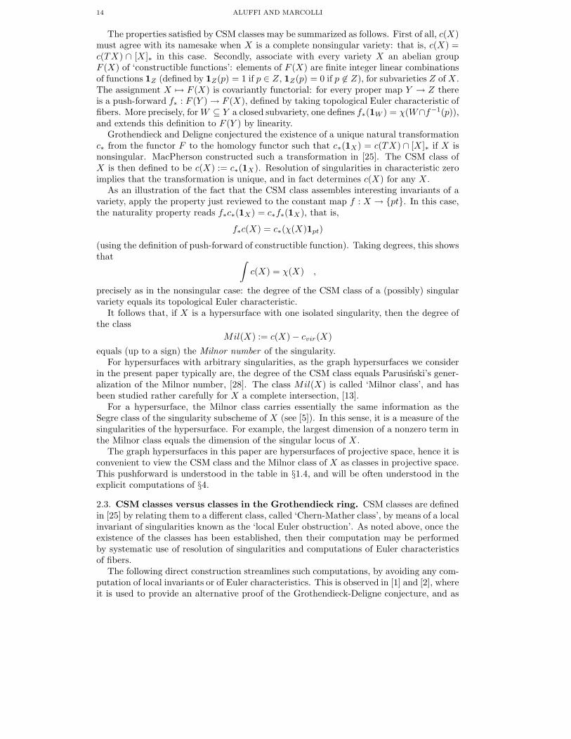
A direct computation using the Macaulay2 program [20] for characteristic classes de-veloped in [4] shows, for the first three examples in this series of graphs depicted in Figure3, the following invariants (see §2 for precise definitions).
n 3 4 5
ΨΓ t1t2 + t2t3 + t1t3 t1t2t3 + t1t2t4+ t1t2t3t4 + t1t2t3t5+t1t3t4 + t2t3t4 t1t2t4t5 + t1t3t4t5 + t2t3t4t5
c(XΓ) 2H2 + 2H 5H3 + 3H2 + 3H 4H4 + 14H3 + 4H2 + 4H
Mil(XΓ) 0 −4H3 60H4 − 10H3
χ(XΓ) 2 5 4
Here H denotes the hyperplane class and c(XΓ) is the Chern–Schwartz–MacPhersonclass of the hypersurface pushed forward to the ambient projective space. We also show theMilnor class, which measures the discrepancy between the Chern–Schwartz–MacPhersonclass and the Fulton class, that is, between the characteristic class of the singular hyper-surface XΓ = ΨΓ = 0 and the class of a smooth deformation. We also display the valueof the Euler characteristic, which one can read off the CSM class. The reader can pausemomentarily to consider the CSM classes reported in the three examples above and noticethat they suggest a general formula for this family of graphs, where the coefficient of Hk
in the CSM class for the n-th hypersurface XΓnis given by the formula
(1.26)
(
n
k
)
−
(
n − 1
k
)
=
(
n − 1
k − 1
)
if k is even
(
n
k
)
+
(
n − 1
k
)
if k is odd
for 1 < k < n, and n − 1 for k = 1. Thus, for example, for n ≥ 3 the Euler characteristicχ(XΓn
) of the n-th banana hypersurface fits the pattern
(1.27) χ(XΓn) = n + (−1)n.
This is indeed the correct formula for the CSM class that will be proved in §4 below.The sample case reported here already exhibits an interesting feature, which we encounteragain in the general formula of §4 and which seems confirmed by computations carried outalgorithmically on other sample graphs from different families of Feynman graphs, namelythe unexpected positivity of the coefficients of the Chern–Schwartz–MacPherson classes.Notice that a similar instance of positivity of the CSM classes arises in another case ofvarieties with a strong combinatorial flavor, namely the case of the Schubert varietiesconsidered in [7]. At present we do not have a conceptual explanation for this positivityphenomenon, but we can state the following tentative guess, based on the sparse numericaland theoretical evidence gathered so far.
Conjecture 1.5. The coefficients of all the powers Hk in the CSM class of an arbitrarygraph hypersurface XΓ are non-negative.

10 ALUFFI AND MARCOLLI
For the general element Γn in the family of the banana graphs, the graph hypersurfaceXΓn
in Pn−1 is defined by the vanishing of the graph polynomial
(1.28) ΨΓn= t1 · · · tn(
1
t1+ · · · +
1
tn).
This is easily seen, since in this case spanning trees consist of a single edge connecting thetwo vertices. Equivalently, one can see this in terms of the matrix MΓ(t).
Lemma 1.6. For the n-th banana graph Γn, the matrix MΓn(t) is of the form
(1.29) MΓn(t) =
t1 + t2 −t2 0 0 · · · 0−t2 t2 + t3 −t3 0 00 −t3 t3 + t4 −t4 00 0 −t4 t4 + t5 0...
......
0 0 0 0 · · · tn−1 + tn
.
Proof. In fact, if we choose as a basis of the first cohomology of the graph Γn the obviousone consisting of the ` = n− 1 loops ei ∪−ei+1, with i = 1, . . . , n− 1, we obtain that then × (n − 1)-matrix ηik is of the form
ηik =
1 0 0 0 0 · · ·−1 1 0 0 0 · · ·
0 −1 1 0 0 · · ·0 0 −1 1 0 · · ·0 0 0 −1 1 · · ·
.
Thus, the matrix (MΓ)rk(t) =∑
i tiηriηik has the form (1.29). It is easy to check that thisindeed has determinant given by (1.28). In fact, from (1.29) one sees that the determinantsatisfies
det MΓn(t) = (tn−1 + tn) det MΓn−1
(t) − t2n−1 det MΓn−2(t).
It then follows by induction that the determinant satisfies the recursive relation
(1.30) det MΓn(t) = tn det MΓn−1
(t) + t1 · · · tn−1.
In fact, assuming the above for n − 1 we obtain
det MΓn(t) = tn det MΓn−1
(t) + t2n−1 det MΓn−2(t) + t1 · · · tn−1 − t2n−1 det MΓn−2
(t).
It is then clear that det MΓn(t) = ΨΓn
(t), with the latter given by the formula (1.28),since this also clearly satisfies the same recursion (1.30).
The dual graph Γ∨n is just a polygon with n vertices and we can identify the hypersurface
XΓ∨
nin Pn−1 with the hyperplane L defined in (1.20).
We rephrase here the statement of Corollary 1.4 in the special case of the banana graphs,since it will be very useful in our explicit computations of §§3 and 4 below.
Lemma 1.7. The n-th banana graph hypersurface is XΓn= π2(π
−11 (L)), with πi : G(C) →
Pn−1, for i = 1, 2, as in (1.17). The Cremona transformation C restricts to a (biregular)isomorphism
(1.31) C : L r Σn → XΓnr Σn.
The map π2 : G(C) → Pn−1 of (1.17) restricts to an isomorphism
(1.32) π2 : π−11 (L r Σn) → XΓn
r Σn.

BANANA MOTIVES 11
Figure 4. Banana graphs with external edges
In order to compute the Feynman integral (1.9), we view the banana graphs Γn not asvacuum bubbles, but as endowed with a number of external edges, as in Figure 4. It doesnot matter how many external edges we attach. This will depend on which scalar fieldtheory the graph belongs to, but the resulting integral is unaffected by this, as long as wehave nonzero external momenta flowing through the graph.
Lemma 1.8. The Feynman integral (1.9) for the banana graphs Γn is of the form
(1.33) U(Γ, p) =Γ((1 − D/2)(n − 1) + 1)C(p)
(4π)(n−1)D/2
∫
σn
(t1 · · · tn)(D
2−1)(n−1)−1 ωn
ΨΓ(t)(D
2−1)n
,
with the function of the external momenta given by C(p) = (∑
Pv)2, with v being eitherone of the two vertices of the graph Γn and Pv =
∑
e∈Eext(Γn),t(e)=v pe.
Proof. The result is immediate from (1.9), using n = ` + 1 and the fact that the onlycut-set for the banana graph Γn consists of the union of all the edges, so that
PΓ(t, p) = C(p) t1 · · · tn.
For example, in the case with n = 2 and D ∈ 2N, D ≥ 4, the integral (up to a divergentGamma factor Γ(2−D/2)4π−D/2) reduces to the computation of the convergent integral
∫
[0,1]
(t(1 − t))D/2−2dt =((D
2 − 2)!)2
(D − 3)!.
In general, apart from poles of the Gamma function, divergences may arise from theintersections of the domain of integration σn with the graph hypersurface XΓn
.
Lemma 1.9. The intersection of the domain of integration σn with the graph hypersurfaceXΓn
happens along σn ∩ Sn in the algebraic simplex Σn.
Proof. The polynomial ΨΓ(t) ≥ 0 for t ∈ Rn+ and by the explicit form (1.28) of the
polynomial, one can see that zeros will only occur when at least two of the coordinatesvanish, i.e. along the intersection of σn with the scheme of singularities Sn of Σn (cf.Lemma 3.8 below).
One procedure to deal with this source of divergences is to work on blowups of Pn−1
along this singular locus (cf. [11], [10]). In [26] another possible method of regularizationfor integrals of the form (1.33) which takes care of the singularities of the integral on σn
(the pole of the Gamma function needs to be addressed separately) was proposed, basedon replacing the integral along σn with an integral that goes around the singularities alongthe fibers of a circle bundle. In general, this type of regularization procedures requires adetailed knowledge of the singularities of the hypersurface XΓ to be carried out, and thatis one of the reasons for introducing invariants of singular varieties in the study of graphhypersurfaces.
12 ALUFFI AND MARCOLLI
2. Characteristic classes and the Grothendieck ring
In order to understand the nature of the part of the cohomology of the graph hy-persurface complement that supports the period corresponding to the Feynman integral(ignoring divergence issues momentarily), one would like to decompose Pn−1 r XΓ intosimpler building blocks. As in §8 of [11], this can be done by looking at the class [XΓ] ofthe graph hypersurface in the Grothendieck ring of motives. One knows by the general re-sult of Belkale–Brosnam [8] that the graph hypersurfaces generate the Grothendieck ring,hence they are quite arbitrarily complex as motives, but one still needs to understandwhether the part of the decomposition that is relevant to the computation of the Feynmanintegral might in fact be of a very special type, e.g. a mixed Tate motive as the evidencesuggests. The family of graphs we consider here is very simple in that respect. In fact,one can see very explicitly that their classes in the Grothendieck ring are combinationsof Tate motives (cf. the formula (3.13) below). One can see this also by looking at theHodge structure. For the graph hypersurfaces of the banana graphs this is described in §8of [10].
Here we describe two ways of analyzing the graph hypersuraces through an additiveinvariant, one as above using the class [XΓ] in the Grothendieck ring, and the other usingthe pushforward of the Chern–Schwartz–MacPherson class of XΓ to the Chow group (orhomology) of the ambient projective space Pn−1. While the first does not depend on anambient space, the latter is sensitive to the specific embedding of XΓ in the projectivespace Pn−1, hence it might conceivably carry a little more information that is useful inrelation to the computation of the Feynman integral on Pn−1 r XΓ. We recall here belowa few basic facts about both constructions. The reader familiar with these generalities canskip directly to the next section.
2.1. The Grothendieck ring. Let VK denote the category of algebraic varieties over afield K. The Grothendieck ring K0(VK) is the abelian group generated by isomorphismclasses [X ] of varieties, with the relation
(2.1) [X ] = [Y ] + [X r Y ],
for Y ⊂ X closed. It is made into a ring by the product [X × Y ] = [X ][Y ].An additive invariant is a map χ : VK → R, with values in a commutative ring R,
satisfying χ(X) = χ(Y ) if X ∼= Y are isomorphic, χ(X) = χ(Y ) + χ(X r Y ) for Y ⊂ Xclosed, and χ(X × Y ) = χ(X)χ(Y ). The Euler characteristic is the prototype exampleof such an invariant. Assigning an additive invariant with values in R is equivalent toassigning a ring homomorphism χ : K0(VK) → R.
Let MK be the pseudo-abelian category of (Chow) motives over K. We write theobjects of MK in the form (X, p, m), with X a smooth projective variety over K, p =p2 ∈ End(X) a projector, and m ∈ Z accounting for the twist by powers of the Tate motiveQ(1). Let K0(MK) denote the Grothendieck ring of the category MK of motives. Theresults of [19] show that, for K of characteristic zero, there exists an additive invariantχ : VK → K0(MK). This assigns to a smooth projective variety X the class χ(X) =[(X, id, 0)] ∈ K0(MK), while for X a general variety it assigns a complex W (X) in thecategory of complexes over MK , which is homotopy equivalent to a bounded complexwhose class in K0(MK) defines the value χ(X). This defines a ring homomorphism
(2.2) χ : K0(VK) → K0(MK).
If L denotes the class L = [A1] ∈ K0(VK) then its image in K0(MK) is the Lefschetzmotive L = Q(−1) = [(Spec(K), id,−1)]. Since the Lefschetz motive is invertible inK0(MK), its inverse being the Tate motive Q(1), the ring homomorphism (2.2) induces a

BANANA MOTIVES 13
ring homomorphism
(2.3) χ : K0(VK)[L−1] → K0(MK).
Thus, in the following we can either regard the classes [XΓ] of the graph hypersurfaces inthe Grothendieck ring of varieties K0(VK) or, under the homomorphism (2.2), as elementsin the Grothendieck ring of motives K0(MK). We will no longer make this distinctionexplicit in the following.
2.2. CSM classes as a measure of singularities. The Chern class of a nonsingularcomplete variety V is the ‘total homology Chern class’ of its tangent bundle. We writec(V ) := c(TV ) ∩ [V ]∗ to indicate the result of applying the Chern class of the tangentbundle of V to the fundamental class [V ]∗ of V . (We use the notation [V ]∗ rather than themore common [V ] in order to avoid any confusion with the class of V in the Grothendieckgroup.)
The class c(V ) resides naturally in the Chow group A∗V . For the purpose of this paper,the reader will miss nothing by replacing A∗V with ordinary homology.
The Chern class of a variety V is a class of evident geometric significance: for ex-ample, the degree of its zero-dimensional component agrees with the topological Eulercharacteristic of V . This follows essentially from the Poincare-Hopf theorem:
∫
c(TV ) ∩ [V ]∗ = χ(V ) .
It is natural to ask whether there are analogs of the Chern class defined for possiblysingular varieties, for which a tangent bundle is not necessarily available.
Somewhat surprisingly, one finds that there are several possible definitions, each ‘natu-ral’ for different reasons, and all agreeing with each other in the nonsingular case. If X isa complete intersection in a nonsingular variety V , it is reasonable to consider the Fultonclass
cvir(X) :=c(TV )
c(NXV )∩ [X ]∗ ,
where NXV denotes the normal bundle to X in V . Up to natural identifications, this isthe Chern class of a smoothing of X (when a smoothing exists), and in particular it agreeswith c(X) if X is nonsingular. It is an interesting fact that this class is independent ofthe realization of X as a complete intersection: that is, it is independent of the ambient
nonsingular variety V . In other words, c(TV )c(NXV ) behaves as the class of a ‘virtual tangent
bundle’ to X . Its definition can in fact be extended (and in more than one way) toarbitrary varieties, see §4.2.6 in [18].
The class cvir(X) is in a sense unaffected by the singularities of X : for a hypersurfaceX in a nonsingular variety V , it is determined by the class of X as a divisor in V .
A much more refined invariant is the Chern-Schwartz-MacPherson (CSM) class of X ,which depends more crucially on the singularities of X , and which we will use as a measureof the singularities by comparison with cvir(X).
The name of the class retains some of its history. In the mid-60s, M.-H. Schwartz([29], [30]) introduced a class extending to singular varieties Poincare-Hopf-type results,by studying tangent frames emanating radially from the singularities. Independently ofSchwartz’ work, Grothendieck and Deligne conjectured a theory of characteristic classesfitting a tight functorial prescription, and in the early 70s R. MacPherson constructed aclass satisfying this requirement ([25]). It was later proved by J.-P. Brasselet and M.-H. Schwartz ([14]) that the classes agree.
In this paper we denote the Chern-Schwartz-MacPherson class of a singular variety Xsimply by c(X) (the notation cSM (X) is frequently used in the literature).
14 ALUFFI AND MARCOLLI
The properties satisfied by CSM classes may be summarized as follows. First of all, c(X)must agree with its namesake when X is a complete nonsingular variety: that is, c(X) =c(TX) ∩ [X ]∗ in this case. Secondly, associate with every variety X an abelian groupF (X) of ‘constructible functions’: elements of F (X) are finite integer linear combinationsof functions 1Z (defined by 1Z(p) = 1 if p ∈ Z, 1Z(p) = 0 if p 6∈ Z), for subvarieties Z of X .The assignment X 7→ F (X) is covariantly functorial: for every proper map Y → Z thereis a push-forward f∗ : F (Y ) → F (X), defined by taking topological Euler characteristic offibers. More precisely, for W ⊆ Y a closed subvariety, one defines f∗(1W ) = χ(W∩f−1(p)),and extends this definition to F (Y ) by linearity.
Grothendieck and Deligne conjectured the existence of a unique natural transformationc∗ from the functor F to the homology functor such that c∗(1X) = c(TX) ∩ [X ]∗ if X isnonsingular. MacPherson constructed such a transformation in [25]. The CSM class ofX is then defined to be c(X) := c∗(1X). Resolution of singularities in characteristic zeroimplies that the transformation is unique, and in fact determines c(X) for any X .
As an illustration of the fact that the CSM class assembles interesting invariants of avariety, apply the property just reviewed to the constant map f : X → pt. In this case,the naturality property reads f∗c∗(1X) = c∗f∗(1X ), that is,
f∗c(X) = c∗(χ(X)1pt)
(using the definition of push-forward of constructible function). Taking degrees, this showsthat
∫
c(X) = χ(X) ,
precisely as in the nonsingular case: the degree of the CSM class of a (possibly) singularvariety equals its topological Euler characteristic.
It follows that, if X is a hypersurface with one isolated singularity, then the degree ofthe class
Mil(X) := c(X) − cvir(X)
equals (up to a sign) the Milnor number of the singularity.For hypersurfaces with arbitrary singularities, as the graph hypersurfaces we consider
in the present paper typically are, the degree of the CSM class equals Parusinski’s gener-alization of the Milnor number, [28]. The class Mil(X) is called ‘Milnor class’, and hasbeen studied rather carefully for X a complete intersection, [13].
For a hypersurface, the Milnor class carries essentially the same information as theSegre class of the singularity subscheme of X (see [5]). In this sense, it is a measure of thesingularities of the hypersurface. For example, the largest dimension of a nonzero term inthe Milnor class equals the dimension of the singular locus of X .
The graph hypersurfaces in this paper are hypersurfaces of projective space, hence it isconvenient to view the CSM class and the Milnor class of X as classes in projective space.This pushforward is understood in the table in §1.4, and will be often understood in theexplicit computations of §4.
2.3. CSM classes versus classes in the Grothendieck ring. CSM classes are definedin [25] by relating them to a different class, called ‘Chern-Mather class’, by means of a localinvariant of singularities known as the ‘local Euler obstruction’. As noted above, once theexistence of the classes has been established, then their computation may be performedby systematic use of resolution of singularities and computations of Euler characteristicsof fibers.
The following direct construction streamlines such computations, by avoiding any com-putation of local invariants or of Euler characteristics. This is observed in [1] and [2], whereit is used to provide an alternative proof of the Grothendieck-Deligne conjecture, and as
BANANA MOTIVES 15
the basis of a generalization of the functoriality of CSM classes to possibly non-propermorphisms.
Given a variety X , let Zi be a finite collection of locally closed, nonsingular subvarietiessuch that X = qiZi. For each i, let νi : Wi → Zi be a resolution of singularities of theclosure of Zi in X , such that the complement Zi r Zi pulls back to a divisor with normalcrossings Ei on Wi. Then
c(X) =∑
i
νi∗c(TWi(− logEi)) ∩ [Wi]∗ .
Here the bundle TWi(− log Ei) is the dual of the bundle Ω1Wi
(log Ei) of differential formson Wi with logarithmic poles along Ei. Each term
(2.4) νi∗c(TWi(− logEi)) ∩ [Wi]∗
computes the contribution c(1Zi) to the CSM class of X due to the (possibly) non-compact
subvariety Zi.We will use this formulation in terms of duals of sheaves of forms with logarithmic poles
to obtain the results of §4 below.By abuse of notation, we denote by c(Z) ∈ A∗V the class so defined, for any locally
closed subset Z of a large ambient variety V . With this notion in hand, note that if Y ⊆ Xare (closed) subvarieties of V , then
c(X) = c(Y ) + c(X r Y ) ,
where push-forwards are, as usual, understood. This relation is very reminiscent of thebasic relation (2.1) that holds in the Grothendieck group of varieties (see §2.1). At thesame time, CSM classes satisfy a ‘product formula’ analogous to the definition of productin the Grothendieck ring ([24], [1]).
Moreover, CSM classes satisfy an ‘embedded inclusion-exclusion’ principle. Namely, ifX1 and X2 are subvarieties of a variety V , then
c(X1 ∪ X2) = c(X1) + c(X2) − c(X1 ∩ X2).
This is clear both from the construction presented above and from the basic functorialityproperty.
In short, there is an intriguing parallel between operations in the Grothendieck group ofvarieties and manipulations of CSM classes. This parallel cannot be taken too far, since the‘embedded’ Chern-Schwartz-MacPherson treated here is not an invariant of isomorphismclasses.
Example 2.1. Let Z1 and Z2 be, respectively, a linearly embedded P1 and a nonsingularconic in P2. Denoting by H the hyperplane class in P2, we find
c(Z1) = (H + 2H2) · [P2]∗ and c(Z2) = (2H + 2H2) · [P2]∗
while of course [Z1] = [Z2] as classes in the Grothendieck group.
Thus, in particular, the CSM class c(X) does not define an additive invariant in thesense of §2.1 and does not factor through the Grothendieck group, as the example aboveshows.
In certain situations it is however possible to establish a sharp correspondence betweenCSM classes and classes in the Grothendieck group. For the next result, we adopt therather unorthodox notation H−r for the class [Pr]∗ of a linear subspace of a given projectivespace. Thus, 1 stands for the class of a point, [P0]∗, and the negative exponents areconsistent with the fact that if H denotes the hyperplane class then Hr · [Pr]∗ = [P0]∗.

16 ALUFFI AND MARCOLLI
Proposition 2.2. Let X be a subset of projective space obtained by unions, intersections,differences of linearly embedded subspaces. With notation as above, assume
c(X) =∑
aiH−i .
Then the class of X in the Grothendieck group of varieties equals
[X ] =∑
aiTi,
where T = [Gm] is the class of the multiplicative group, see §3.
Thus, adopting a variable T = H−1 in the CSM environment, and T = T in theGrothendieck group environment, the classes corresponding to subsets as specified in thestatement would match precisely.
Proof. The formula holds for a linearly embedded X = Pr, since
c(Pr) = ((1 + H)r+1 − Hr+1) · [Pr]∗ = ((1 + H)r+1 − Hr+1) · H−r =(1 + H−1)r+1 − 1
H−1
and (see (3.1) below)
[Pr] =(1 + T)r+1 − 1
T.
Since embedded CSM classes and classes in the Grothendieck group both satisfy inclusion-exclusion, this relation extend to all sets obtained by ordinary set-theoretic operationsperformed on linearly embedded subspaces, and the statement follows.
Proposition 2.2 applies, for example, to the case of hyperplane arrangements in PN : fora hyperplane arrangement, the information carried by the class in the Grothendieck groupof varieties is precisely the same as the information carried by the embedded CSM class.These classes reflect in a subtle way the combinatorics of the arrangement.
In a more general setting, it is still possible to enhance the information carried by theCSM class in such a way as to establish a tight connection between the two environments.For example, CSM classes can be treated within a framework with strong similarities withmotivic integration, [3].
In any case, one should expect that, in many examples, the work needed to compute aCSM class should also lead to a computation of a class in the Grothendieck group. Thecomputations in §3 and §4 in this paper will confirm this expectation for the hypersurfacescorresponding to banana graphs.
3. Banana graphs and their motives
In this section we give an explicit formula for the classes [XΓn] of the banana graph
hypersurfaces XΓnin the Grothendieck ring. The procedure we adopt to carry out the
computation is the following. We use the Cremona transformation of (1.17). Consider thealgebraic simplex Σn placed in the Pn−1 on the right-hand-side of the diagram (1.17). Thecomplement of this Σn in the graph hypersurface XΓn
is isomorphic to the complement ofthe same union Σn in the corresponding hyperplane L in the Pn−1 on the left-hand-sideof (1.17), by Lemma 1.7 above. So this provides the easy part of the computation, andone then has to give explicitly the classes of the intersections of the two hypersurfaceswith the union of the coordinate hyperplanes. The final formula for the class [XΓn
] has asimple expression in terms of the classes of tori Tk, with T := [A1] − [A0] the class of themultiplicative group Gm. Then Tn−1 is the class of the complement of Σn inside Pn−1.
In the following we let 1 denote the class of a point [A0]. We use the standard notationL for the class [A1] of the affine line (the Lefschetz motive). We also denote, as above, byΣn the union of coordinate hyperplanes in Pn−1 and by Sn its singularity locus.
BANANA MOTIVES 17
First notice the following simple identity in the Grothendieck ring.
(3.1) [Pr] =
r∑
i=0
Lr =1 − Lr+1
1 − L=
(1 + T)r+1 − 1
T.
This expression can be thought of as taking place in a localization of the Grothendieckring, but in fact this is not really necessary if we take these fractions as just shorthand fortheir unambiguous expansions.
We introduce the following notation. Suppose given a class C in the Grothendieck ringwhich can be written in the form
(3.2) C = a0[P0] + a1[P
1] + a2[P2] + · · ·
To such a class we assign a polynomial
(3.3) f(P ) = a0 + a1P + a2P2 + · · ·
Remark 3.1. Notice that the formal variable P does not define an element in theGrothendieck ring, since one sees easily that P iP j 6= P i+j . In fact, the variables P i
satisfy a different multiplication rule, which we denote by • and which is given by
(3.4) P i • P j = P i+j + P i+j−1 + · · · + P j − P i−1 − · · · − 1
and which recovers in this way the class [Pi × Pj ]. This follows from Lemma 3.2, byconverting each of the two factors into the corresponding expressions in T, multiplyingthese as classes in the Grothendieck ring, and then converting the result back in terms ofthe variables P i.
Lemma 3.2. Let C be a class in the Grothendieck ring that can be written in terms ofclasses of projective spaces in the form (3.2). One can convert it into a function of theclass T of the form
(3.5) C =(1 + T)f(1 + T) − f(1)
T,
where f is as in (3.3).
Proof. One obtains (3.5) from (3.2) using the expression (3.1) of [Pr] in terms of T. Infact, (3.5) gives the expression of [Pr] as a function of T when applied to f(P ) = P r.
Conversely, we have a similar way to convert classes in the Grothendieck ring that canbe expressed as a function of the torus class into a function of the classes of projectivespaces.
Lemma 3.3. Suppose given a class C in the Grothendieck ring that can be written as afunction of the torus class T, by a polynomial expression C = g(T). Then one obtains anexpression of C in terms of the classes of projective spaces [Pr] by first taking the function
(3.6)(P − 1)g(P − 1) + g(−1)
P
and then replacing P r by the class [Pr] in the expansion of (3.6) as a polynomial in theformal variable P .
Proof. The result is obtained by solving for f in (3.5), which yields the formula (3.6).
Next we define an operation on classes of the form C = g(T), which one can think ofas “taking a hyperplane section”. Notice that literally taking a hyperplane section is nota well defined operation at the level of the Grothendieck ring, but it does make sense onclasses that are constructed from linearly embedded subspaces of a projective space, as isthe case we are considering.

18 ALUFFI AND MARCOLLI
Lemma 3.4. The transformation
(3.7) H : g(T) 7→g(T) − g(−1)
T + 1
gives an operation on the set of classes in the Grothendieck ring that are polynomial func-tions of the torus class T. In terms of classes [Pr] it corresponds to mapping [P0] to zeroand [Pr] to [Pr−1] for r ≥ 1.
Proof. One can see that, for g(T) = [Pr] = (1+T)r+1−1
T, we have
g(T) − g(−1)
T + 1=
(1+T)r+1−1
T− 1
T + 1=
(1 + T)r − 1
T= [Pr−1],
or 0 if r = 0, so that the operation (3.7) indeed corresponds to taking a hyperplane section.The operation is linear in g, viewed as a linear combination of classes of projective spaces,so it works for arbitrary g.
We then have the following preliminary result.
Lemma 3.5. The class of Σr+1 ⊂ Pr in the Grothendieck ring is of the form
(3.8) [Σr+1] =(1 + T)r+1 − 1 − Tr+1
T=
r∑
i=1
(
r + 1
i
)
Tr−i.
Intersecting with a transversal hyperplane L then gives
(3.9) [L ∩ Σr+1] =(1 + T)r − 1
T− Tr−1 + Tr−2 − Tr−3 + · · · ± 1.
Proof. The class of the complement of Σr+1 in Pr is the torus class Tr. In fact, thecomplement of Σr+1 consists of all (r + 1)-tuples (1: ∗ : · · · :∗), where each ∗ is a nonzeroelement of the ground field. It then follows directly that the class of Σr+1 has the form(3.8), using the expression (3.1) for the class [Pr]. One then applies the transformation Hof (3.7) to obtain
[L ∩ Σr+1] =(
(1+T)r+1−1−T
r+1
T− −1−(−1)r+1
−1
)
/(T + 1)
= (1+T)r−1
T− T
r−(−1)r
T+1
from which (3.9) follows.
Definition 3.6. The trace Σ′r+1 ⊂ Pr−1 of the algebraic simplex Σr+1 ⊂ Pr is the in-
tersection of Σr+1 with a general hyperplane. It is a union of r + 1 hyperplanes in Pr−1
meeting with normal crossings.
For instance, Σ′4 consists of the transversal union of four lines as in Figure 5 and by
(3.9) its class is
[Σ′4] =
(1 + T)3 − 1
T− T2 + T − 1 = 4T + 2.
The first part of the computation of the class of the graph hypersurface XΓnfor the
banana graph Γn is then given by the following result.
Proposition 3.7. Let XΓn⊂ Pn−1 be the hypersurface of the n-th banana graph Γn. Then
(3.10) [XΓnr Σn] = Tn−2 − Tn−3 + Tn−4 − · · · + (−1)n.

BANANA MOTIVES 19
Figure 5. The trace Σ′4 ⊂ P2 of the algebraic simplex Σ4 ⊂ P3
Proof. We know by Lemma 1.7 that XΓnrΣn
∼= LrΣn via the Cremona transformation,with L = Pn−2 the hyperplane (1.20). This hyperplane intersects Σn transversely, so that(3.9) applies and gives
[L r Σn] = [L] − [L ∩ Σn] =Tn−1 − (−1)n−1
T + 1.
Next we examine how the graph hypersurface XΓnintersects the algebraic simplex Σn.
Lemma 3.8. The graph hypersurface XΓnintersects the algebraic simplex Σn ⊂ Pn−1
along the singularity subscheme Sn of Σn.
Proof. One can see this directly by comparing the defining equation (1.28) of XΓnwith
the ideal ISnof (1.19) of the singularity subscheme Sn of Σn.
The class in the Grothendieck ring of the singular locus Sn of Σn is given by thefollowing result.
Lemma 3.9. The class of Sr+1 ⊂ Pr is given by
(3.11) [Sr+1] = [Σr+1] − (r + 1)Tr−1 =
r∑
i=2
(
r + 1
i
)
Tr−i.
Proof. Each coordinate hyperplane Pr−1 in Σr+1 ⊂ Pr intersects the others along its ownalgebraic simplex Σr. Thus, to obtain the class of Sr+1 from the class of Σr+1 in theGrothendieck ring we just need to subtract the class of the r + 1 complements of Σr inthe r + 1 components of Σr+1. We then have
[Sr+1] = [Σr+1] − (r + 1)Tr−1 =(1 + T)r+1 − 1 − (r + 1)Tr − Tr+1
T.
This gives the formula (3.11).
We then have the following result.

20 ALUFFI AND MARCOLLI
Theorem 3.10. The class in the Grothendieck ring of the graph hypersurface XΓnof the
banana graph Γn is given by
(3.12) [XΓn] =
(1 + T)n − 1
T−
Tn − (−1)n
T + 1− n Tn−2.
Proof. We write the class [XΓn] in the form
[XΓn] = [XΓn
r Σn] + [Sn].
Using the results of Lemma 3.9 and Proposition 3.7 we write this as
=Tn−1 − (−1)n−1
T + 1+
(1 + T)n − 1 − nTn−1 − Tn
T,
from which (3.12) follows.
The formula (3.12) expresses the class [XΓn] as
[XΓn] = [Σ′
n] − nTn−2,
i.e. as the class of the union Σ′n of n hyperplanes meeting with normal crossings (as in
Definition 3.6), corrected by n times the class of an n − 2-dimensional torus.
Example 3.11. In the case n = 3 of Figure 3, (3.12) shows that the class of the hyper-surface XΓ3
⊂ P2 is equal to the class of the union of four transversal lines, minus threetimes a 1-dimensional torus, i.e. that we have
[XΓ3] = 4T + 2 − 3T = T + 2 = [P1].
This can also be seen directly from the fact that the equation
ΨΓ3= t1t2 + t2t3 + t1t3 = 0
defines a nonsingular conic in the plane.
Example 3.12. In the case n = 4 of Figure 3, the hypersurface XΓ4is a cubic surface in
P3 with four singular points. The class in the Grothendieck ring is
[XΓ4] = T2 + 5T + 5.
In terms of the Lefschetz motive L, the formula (3.12) reads equivalently as
(3.13) [XΓn] =
Ln − 1
L − 1−
(L − 1)n − (−1)n
L− n (L − 1)n−2.
In the context of parametric Feynman integrals, it is the complement of the graphhypersurface in Pn−1 that supports the period computed by the Feynman integral. Thus,in general, one is interested in the explicit expression for the motive of the complement.It so happens that in the particular case of the banana graphs the expression for the classof the hypersurface complement is in fact simpler than that of the hypersurface itself.
Corollary 3.13. The class of the hypersurface complement Pn−1 r XΓnis given by
(3.14)[Pn−1 r XΓn
] = Tn−(−1)n
T+1 + n Tn−2
= Tn−1 + (n − 1)Tn−2 + Tn−3 − Tn−4 + Tn−5 + · · · ± 1.
Proof. By (3.1) we see that the first term in (3.12) is in fact the class [Pn−1], hence theclass [Pn−1 r XΓn
] = [Pn−1] − [XΓn] is given by (3.14)
Corollary 3.14. The Euler characteristic of XΓnis given by the formula (1.27).
BANANA MOTIVES 21
Proof. The Euler characteristic is an additive invariant, hence it determines a ring ho-momorphism from the Grothendieck ring of varieties to the integers. Moreover, tori havezero Euler characteristic, so that χ(Tr) = 0 for all r ≥ 1. Then the formula (3.14) for theclass of the hypersurface complement shows that
χ(Pn−1 r XΓn) = χ(Tn−1) + (n − 1)χ(Tn−2) + χ(Tn−3) − · · · ± 1 = (−1)n−1.
Since χ(Pn−1) = n we obtain
χ(XΓn) = χ(Pn−1) − χ(Pn−1 r XΓn
) = n + (−1)n
as in (1.27).
In §4 below, we derive the same Euler characteristic formula in a different way, fromthe calculation of the CSM class of XΓn
.
Remark 3.15. Notice that, if we expand in (3.12) the first term in the form [Pn−1] =Tn−1+nTn−2+. . . , we see that the dominant term in [XΓn
] is Tn−2. This is not surprising,since for the banana graphs the hypersurfaces XΓn
are rational.
Remark 3.16. The previous remark explains the appearance of a term nTn−2 in theexpression (3.14). The remaining terms are an alternating sum of tori. This term can beviewed as
(3.15)Tn − (−1)n
T + 1=
g(T) − g(−1)
T + 1,
for g(T) = Tn. According to Lemma 3.4, this is the class of the hyperplane section ofthe complement of the algebraic simplex Σn+1 in Pn. However, how geometrically onecan associate a Pn to a graph hypersurface XΓn
⊂ Pn−1 is unclear, so that a satisfactoryconceptual explanation of the occurrence of (3.15) in (3.14) is still missing.
For completeness we also give the explicit formula of the class (3.14) written in termsof classes [Pr].
Corollary 3.17. In terms of classes of projective spaces the class [Pn−1 r XΓn] is given
by
(3.16) [Pn−1 r XΓn] =
n−1∑
k=0
(
n + 1
k + 2
)
(−1)n−1−k [Pk] + n
n−2∑
k=0
(
n − 1
k + 1
)
(−1)n−2−k [Pk].
Proof. The formula (3.16) is obtained easily using the transformation rules of Lemma 3.3to go from expressions in T to expressions in [Pr], so that
(Tn − (−1)n)/(T + 1) 7→(
(P − 1) (P−1)n−(−1)n
P + n(−1)n−1)
/P
=(
(P − 1)n+1 − (n + 1)(−1)nP − (−1)n+1)
/P 2
=∑n−1
k=0
(
n+1k+2
)
(−1)n−1−k [Pk],
and for the second term
n Tn−2 7→ n(
(P − 1)(P − 1)n−2 + (−1)n−2)
/P
= n(
(P − 1)n−1 − (−1)n−1)
/P
= n∑n−2
k=0
(
n−1k+1
)
(−1)n−2−k [Pk].

22 ALUFFI AND MARCOLLI
3.1. Classes of dual graphs. In the result obtained above, we used essentially the rela-tion between the graph hypersurface XΓn
and the hypersurface of the dual graph, which is,in this case, a hyperplane. More generally, although one cannot obtain an explicit formula,one can observe that for any given planar graph the relation between the hypersurface XΓ
of the graph and that of the dual graph XΓ∨ gives a relation between the classes in theGrothendieck ring, which can be expressed as follows.
Proposition 3.18. Let Γ be a planar graph with n = #E(Γ) and let Γ∨ be a dual graph.Then the classes in the Grothendieck ring satisfy
(3.17) [XΓ] − [XΓ∨ ] = [Σn ∩ XΓ] − [Σn ∩ XΓ∨ ].
Proof. The result is a direct consequence of Corollary 1.4.
4. CSM classes for banana graphs
We now give an explicit formula for the Chern–Schwartz–MacPherson class of the hy-persurfaces of the banana graphs, for an arbitrary number of edges.
The computation of the CSM class is substantially more involved than the computationof the class in the Grothendieck ring we obtained in the previous section, although the twocarry strong formal similarities, due to the fact that both are based on a similar inclusion–exclusion principle. In fact, the information carried by the CSM class is more refined thanthe decomposition in the Grothendieck ring of varieties, as it captures more sophisticatedinformation on how the building blocks are embedded in the ambient space. This will beillustrated rather clearly by our explicit computations. In particular, the explicit formulafor the CSM class uses in an essential way a special formula for pullbacks of differentialforms with logarithmic poles.
In order to avoid any possible confusion between homology classes and classes in theGrothendieck ring (even though the context should suffice to distinguish them), we usehere as in §2.2 the notation [Pr]∗ for homology classes or classes in the Chow group (inan ambient Pn−1), while reserving the symbol [Pr] for the class in the Grothendieck ring,as already used in §3 above. The homology class [Pr]∗ can be expressed in terms of thehyperplane class H and the ambient Pn−1 as [Pr]∗ = Hn−1−r[Pn−1]∗.
4.1. Characteristic classes of blowups. Let D be a divisor with simple normal cross-ings and nonsingular components Di, i = 1, . . . , r, in a nonsingular variety M . ThenTM(− log(D)) denotes the sheaf of vector fields with logarithmic zeros (i.e. the dual ofthe sheaf Ω1
M (log D) of 1-forms with logarithmic poles). In terms of Chern classes one has(cf. e.g. [3])
c(TM(− logD)) =c(TM)
(1 + D1) · · · (1 + Dr).
This formula has useful applications in the calculation of CSM classes, especially becauseit behaves nicely under pushforwards as shown in [3] and [2]. What we need here is a moresurprising pullback formula, which can be stated as follows.
Theorem 4.1. Let π : W → V be the blowup of a nonsingular variety V along a nonsin-gular subvariety B, with exceptional divisor F . Let Ej , j ∈ J , be nonsingular irreduciblehypersurfaces of V , meeting with normal crossings. Assume that B is cut out by some ofthe Ej ’s. Denote by Fj the proper transform of Ej in W . Then the sheaf of 1-forms withlogarithmic poles along E is preserved by the pullback, namely
(4.1) Ω1M (log(F +
∑
Fj)) = π∗Ω1M (− log(
∑
Ej)).

BANANA MOTIVES 23
Proof. There is an inclusion π∗Ω1M (log(
∑
Ej)) ⊂ Ω1M (log(F +
∑
Fj)), and it suffices tosee that this is an equality locally analytically. To this purpose, choose local coordinatesx1, . . . , xn in V , so that Ej is given by (xj), j = 1, . . . , k. Assume B has ideal (x1, . . . , x`),and choose local parameters y1, . . . , yn in W so that π is expressed by
x1 = y1
x2 = y1y2
· · ·
x` = y1y`
x`+1 = y`+1
· · ·
xn = yn
Then local sections of π∗Ω1(log(∑
Ej)) are spanned by
dy1
y1,
dy1
y1+
dy2
y2, · · · ,
dy1
y1+
dy`
y`,
dy`+1
y`+1, · · · ,
dyn
yn
These clearly span the whole of Ω1(log(F +∑
Fj)), as claimed. Thus, we obtain (4.1).
One derives directly from this result the following formula for Chern classes.
Corollary 4.2. Under the same hypothesis as Theorem 4.1, the Chern classes satisfy
(4.2)c(TW )
(1 + F )∏
j∈J (1 + Fj)∩ [W ] = π∗
(
c(TV )∏
j∈J (1 + Ej)∩ [V ]
)
.
In other words, if B is cut out by a selection of the components Ej , then the pullback ofthe total Chern class of the bundle of vector fields with logarithmic zeros along E equalsthe one of the analogous bundle upstairs.
The main consequence of Theorem 4.1 and Corollary 4.2 which is relevant to the caseof graph hypersurfaces is given by the following application.
Definition 4.3. Let V be a nonsingular variety, and let Ej , j ∈ J , be nonsingular divisorsmeeting with normal crossings in V . A proper birational map π : W → V is a blowupadapted to the divisor with normal crossings if it is the blowup of V along a subvarietyB ⊂ V cut out by some of the Ej ’s.
Notice that W carries a natural divisor with normal crossings, that is, the union of theexceptional divisor F and of the proper transforms Fj of the divisors Ej . The blowupmaps the complement of W to this divisor isomorphically to the complement in V of thedivisor ∪Ej . It makes sense then to talk about a sequence of adapted blowups, by which wemean that each blowup in the sequence is adapted to the corresponding normal crossingdivisor. We then have the following consequence of Theorem 4.1 and Corollary 4.2 above.
Corollary 4.4. Let V be a nonsingular variety, and Ej be nonsingular divisors meetingwith normal crossings in V . Let U denote the complement of the union E = ∪j∈JEj . Letπ : W → V be a proper birational map dominated by a sequence of adapted blowups. Inparticular, π maps π−1(U) isomorphically to U . Then
(4.3) c(1π−1(U)) = π∗c(1U ).
Proof. Let π : V → V be a sequence of adapted morphisms dominating π:
Vα
//
π
@@@@
@@@@
W
π
V
24 ALUFFI AND MARCOLLI
The divisor E = π−1(∪Ej) is then a divisor with normal crossings, and π−1(U) is its
complement in V . By Corollary 4.2, we have the identity
c(T V (− log E)) ∩ [V ] = π∗(c(TV (− log E)) ∩ [V ]) = α∗π∗(c(TV (− log E)) ∩ [V ]).
As in (2.4) of §2.3, this is saying that
c(1π−1(U)) = α∗π∗(c(1U )).
The statement then follows by pushing forward through α (applying MacPherson’s theo-rem), since α∗α
∗ = 1 as α is proper and birational.
The identity of CSM classes happens in the homology (or Chow group) of W . Noticethat we are not assuming here that W is nonsingular. One also has π∗c(1π−1(U)) = c(U)in the homology (Chow group) of V , by MacPherson’s theorem [25] on functoriality ofCSM classes. What is surprising about (4.3) is that for this class of morphisms one cando for pullbacks what functoriality usually does for pushforward.
4.2. Computing the characteristic classes. In this section we give the explicit formulafor the CSM class of the graph hypersurface XΓn
of the banana graph Γn. The procedureis somewhat similar conceptually to the one we used in the computation of the class inthe Grothendieck ring, namely we will use the inclusion–exclusion property of the Chernclass and separate out the contributions of the part of XΓn
that lies in the complementof the algebraic simplex Σn ⊂ Pn−1 and of the intersection XΓn
∩Σn, using the Cremonatransformation to compute the contribution of the first and inclusion-exclusion again tocompute the class of the latter.
As above, let Sn be the singularity subscheme of Σn. We begin by the following pre-liminary result.
Proposition 4.5. The CSM class of Sn is given by
(4.4) c(Sn) = ((1 + H)n − 1 − nH − Hn) · [Pn−1]∗.
Proof. Since Sn is defined by the ideal (1.19) of the codimension two intersections of thecoordinate planes of Pn−1, one can use the inclusion-exclusion property to compute (4.4).Equivalently, one can use the result of [1], which shows that, for a locus that is a union oftoric orbits, the CSM class is a sum of the homology classes of the orbit closures. Thus,one can write the CSM class of Pn−1 as the sum of the CSM class of Sn, the homologyclasses of the coordinate hyperplanes, and the homology class of the whole Pn−1, i.e.
c(Pn−1) = (c(Sn) + nH + 1) · [Pn−1]∗,
where the two latter terms correspond to the classes of the closures of the higher dimen-sional orbits. Since c(Pn−1) = ((1 + H)n − Hn) · [Pn−1]∗, this gives (4.4).
We now concentrate on the complement XΓnrΣn. We again use Lemma 1.7 to describe
this, via the Cremona transformation, in terms of L r Σn, with L the hyperplane (1.20).We have the following result.
Lemma 4.6. Let π1 : G(C) → Pn−1 be as in (1.17). Then
(4.5) c(π−11 (L r Σn)) = π∗
1(c(L r Σn)).
Proof. By Corollary 4.4, it suffices to show that the restriction of π1 to π−1(L) is adaptedto L ∩ Σn. By (2) and (3) of Lemma 1.2, we know that π−1
1 (L) is the blowup of L alongL ∩ Sn, that is, the singularity subscheme of L ∩ Σn. The blowup of a variety alongthe singularity subscheme of a divisor with simple normal crossings is dominated by thesequence of blowups along the intersections of the components of the divisor, in increasingorder of dimension. This sequence is adapted, hence the claim follows. Equivalently, notice

BANANA MOTIVES 25
that π1 : G(C) → Pn−1 is itself dominated by a sequence adapted to Σn. Moreover, L andits proper transform intersect all centers of the blowups in the sequence transversely. Thisalso shows that the restriction of π1 to π−1
1 (L) is adapted to L ∩ Σn.
We have the following result for the CSM class of L r Σn in terms of the homology(Chow group) classes [Pr]∗.
Lemma 4.7. The CSM class of L r Σn is given by
(4.6) c(L r Σn) = [Pn−2]∗ − [Pn−3]∗ + · · · + (−1)n[P0]∗.
Let h denote the homology class of the hyperplane section in the source Pn−1 of diagram(1.17). Then (4.6) is written equivalently as
(4.7) c(L r Σn) = (1 + h)−1h · [Pn−1]∗.
Proof. The divisor Σn has n components with homology class h, hence so does L ∩ Σn.Since the CSM class of a divisor with normal crossings is computed by the Chern class ofthe bundle of vector fields with logarithmic zeros along the components of the divisor, wefind
c(L r Σn) =c(TL) ∩ [L]∗
(1 + h)n=
(1 + h)n−1
(1 + h)nh · [Pn−1]∗.
We then have the following result that gives the formula for c(XΓn).
Theorem 4.8. The (push-forward to Pn−1 of the) CSM class of the banana graph hyper-surface XΓn
is given by
(4.8) c(XΓn) = ((1 + H)n − (1 − H)n−1 − nH − Hn) · [Pn−1]∗.
Proof. Using inclusion-exclusion for CSM classes we have
c(XΓn) = c(XΓn
∩ Σn) + c(XΓnr Σn).
By Lemma 3.8, we know that XΓn∩Σn = Sn, hence the first term is given by (4.4). Thus,
we are reduced to showing that
(4.9) c(XΓnr Σn) = (1 − (1 − H)n−1) · [Pn−1]∗.
Combining Lemmata 4.6 and 4.7, we find
c(XΓnr Σn) = π2∗π
∗1
(
∑n−1i=1 (−1)i−1hi · [Pn−1]∗
)
= π2∗
(
∑n−1i=1 (−1)i−1hi · [G(C)]∗
)
,
where we view h as a divisor class on G(C), suppressing the pullback notation. Let Hdenote the hyperplane class in the target Pn−1 of diagram (1.17), as well as its pullbackto G(C). Notice that, by (1.18), G(C) is a complete intersection of n − 1 hypersurfaces ofhomology class h + H in Pn−1 × Pn−1. Thus, we obtain
c(XΓnr Σn) = π2∗
(
n−1∑
i=1
(−1)i−1hi(h + H)n−1 · [Pn−1 × Pn−1]∗
)
.
Finally, we have to evaluate the pushforward via π2. We can write
c(XΓnr Σn) =
n−1∑
i=1
aiHi · [Pn−1]∗,
where we need to evaluate the integers ai. Since
ai =
∫
Hn−1−i · c(XΓnr Σn),

26 ALUFFI AND MARCOLLI
by the projection formula we obtain
ai =
∫
Hn−1−in−1∑
i=1
(−1)i−1hi(h + H)n−1 · [Pn−1 × Pn−1]∗.
In Pn−1 ×Pn−1, the only nonzero monomial in h, H of degree 2n− 2 is hn−1Hn−1, whichevaluates to 1. Therefore, we have
ai = (−1)i−1 · coefficient of hn−1−iH i in (h + H)n−1 = (−1)i−1
(
n − 1
i
)
.
We then obtain
c(XΓnr Σn) =
∑n−1i=1 aiH
i · [Pn−1]∗
=∑n−1
i=1 (−1)i−1(
n−1i
)
H i · [Pn−1]∗
= (1 − (1 − H)n−1) · [Pn−1]∗.
This gives a different way of computing the topological Euler characteristic of XΓn,
which we already derived from the class in the Grothendieck ring in Corollary 3.14.
Corollary 4.9. The Euler characteristic of the banana graph hypersurface XΓnis given
by the formula (1.27).
Proof. For a projective hypersurface X the value of the Euler characteristic χ(X) can beread off the CSM class as the coefficient of the top degree term. Thus, from (4.8) weobtain χ(XΓn
) = n + (−1)n.
Remark 4.10. The coefficient of Hk in the CSM class is as prescribed in (1.26). Inparticular, these coefficients are positive for all n ≥ 2 and 1 ≤ k ≤ n − 1. Thus, bananagraphs provide an infinite family of graphs for which Conjecture 1.5 holds.
Remark 4.11. As pointed out in §2.3, CSM classes are defined (as classes in the Chowgroup of an ambient variety) for locally closed subsets. It follows from Theorem 4.8 thatthe CSM class of the complement of XΓn
in Pn−1 is
c(Pn−1 r XΓn) = ((1 − H)n−1 + nH) ∩ [Pn−1]∗.
4.3. The CSM class and the class in the Grothendieck ring. We discuss here theformal similarity, as well as the discrepancy, between the expression for the CSM class andthe formula for the class in the Grothendieck ring of the graph hypersurface XΓn
.As noted in Propostion 2.2, the CSM class and the class in the Grothendieck group
carry the same information for subsets of projective space consisting of unions of linearsubspaces. The algebraic simplex, as well as its trace on a transversal hyperplane, aresubsets of this type. Thus, some of the work performed in §§3 and 4 is redundant.
The class [XΓn] of the graph hypersurface XΓn
of the banana graph Γn can be separatedinto two parts, only one of which –the part that comes from the simplex– is linearlyembedded. These two parts are responsible, respectively, for the formal similarity and forthe discrepancy between the expression for the class [XΓn
] and the one for c(XΓn).
In fact, denoting the unorthodox H−1 of Proposition 2.2 by a variable T , the CSM classof XΓn
has the form
(4.10) c(XΓn) =
(1 + T )n − 1
T− (T − 1)n−1 − n T n−2.

BANANA MOTIVES 27
The central term is the one that differs from the expression (3.12). Adopting the samevariable T for the class T of a torus, the discrepancy is measured by the amount
T n − (−1)n
T + 1− (T − 1)n−1.
5. Classes of cones
We make here a general observation which may be useful in other computations of CSMclasses and classes in the Grothendieck ring for graph hypersurfaces. One can observethat often the graph hypersurfaces XΓ happen to be cones over hypersurfaces in smallerprojective spaces.
There are simple operations one can perform on a given graph, which ensure that theresulting graph will correspond to a hypersurface that is a cone. Here is a list:
• Subdividing an edge.• Connecting two graphs by a pair of edges.• Appending a tree to a vertex (in this case the resulting graph will not be 1PI).
One can see easily that in each of these cases the resulting hypersurface is a cone, since inthe first two cases the resulting graph polynomial ΨΓ will depend on two of the variablesonly through their linear combination ti + tj , while in the last case ΨΓ does not dependon the variables of the edges in the tree.
It may then be useful to provide an explicit formula for computing the CSM class andthe class in the Grothendieck ring for cones. The result can be seen as a generalization ofthe simple formula for the Euler characteristic.
Lemma 5.1. Let Ck(X) be a cone in Pn+k of a hypersurface X ⊂ Pn. Then the Eulercharacteristic satisfies
χ(Ck(X)) = χ(X) + k.
Proof. Consider first the case of C(X) = C1(X). We have
C(X) = (X × P1)/(X × pt) = (X × A1) ∪ pt,
from which, by the inclusion-exclusion property of the Euler characteristic we immediatelyobtain χ(C(X)) = χ(X) + 1. The result then follows inductively.
The case of the CSM class is given by the following result.
Proposition 5.2. Let i : X → Pm be a subvariety, and let j : C(X) → Pm+1 be the coneover X. Let H denote the hyperplane class and let
i∗c(X) = f(H) ∩ [Pm]∗
be the CSM class of X expressed in the Chow group (homology) of the ambient Pm. Thenthe CSM class of the cone (in the ambient Pm+1) is given by
(5.1) j∗c(C(X)) = (1 + H)f(H) ∩ [Pm+1]∗ + [P0]∗.
Proof. Let j∗c(C(X)) = g(H) ∩ [Pm+1]∗. Notice that X may be viewed as a generalhyperplane section of C(X). Then, by Claim 1 of [6] we have
f(H) ∩ [Pm]∗ = i∗c(X) = H · (1 + H)−1 ∩ j∗c(C(X)) = H(1 + H)−1g(H) ∩ [Pm+1]∗.
This implies
(5.2) (1 + H)f(H) ∩ [Pm]∗ = g(H) ∩ [Pm]∗.
This determines all the coefficients in g(H) with the exception of the coefficient of Hm+1.The latter equals the Euler characteristic of C(X), hence by Lemma 5.1 this is χ(C(X)) =χ(X) + 1. Thus, we have
coefficient of Hm+1 in g(H) = 1 + coefficient of Hm in f(H) .
28 ALUFFI AND MARCOLLI
Together with (5.2), this implies (5.1).
This result applies to some of the operations on graphs described above. Here, as inthe rest of the paper, we suppress the explicit pushfoward notation i∗ and j∗ in writingCSM classes in the Chow group or homology of the ambient projective space.
Corollary 5.3. Let Γ be a graph with n edges, and let Γ be the graph obtained by subdi-viding an edge or by attaching a tree consisting of a single edge to one of the vertices. Ifthe CSM class of the hypersurface XΓ is of the form c(XΓ) = f(H) ∩ [Pn−1]∗, with f apolynomial of deg(f) ≤ n − 1 in the hyperplane class, then the class of XΓ is given by
c(XΓ) = ((1 + H)f(H) + Hn) ∩ [Pn]∗ .
Proof. The result follows immediately from Proposition 5.2, since in the first case thegraph polynomial ΨΓ depends on a pair of variables ti, tj only through their sum ti + tj ,hence XΓ is a cone over XΓ inside Pn. In the second case the graph polynomial ΨΓ isindependent of the variable of the additional edge and the result follows by the sameargument, since XΓ is then also a cone over XΓ.
The case of attaching an arbitrary tree to a vertex of the graph is obtained by iteratingthe second case of Corollary 5.3.
There are further cases of simple operations on a graph which can be analyzed as aneasy consequence of the formulae for cones:
• Adjoining a loop made of a single edge connecting a vertex to itself.• Doubling a disconnecting edge in a non-1PI graph.
In these cases the resulting graph hypersurface is obtained by first taking a cone over theoriginal hypersurface in one extra dimension and then taking the union with a transversalhyperplane, respectively given by the vanishing of the coordinate corresponding to theloop edge or by the vanishing of the sum ti + tj coming from the pair of parallel edges.We then have the following result.
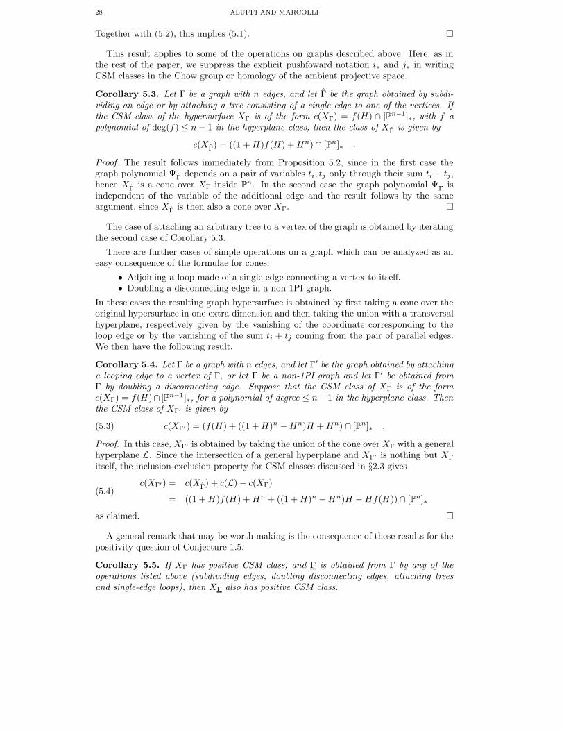
Corollary 5.4. Let Γ be a graph with n edges, and let Γ′ be the graph obtained by attachinga looping edge to a vertex of Γ, or let Γ be a non-1PI graph and let Γ′ be obtained fromΓ by doubling a disconnecting edge. Suppose that the CSM class of XΓ is of the formc(XΓ) = f(H)∩ [Pn−1]∗, for a polynomial of degree ≤ n− 1 in the hyperplane class. Thenthe CSM class of XΓ′ is given by
(5.3) c(XΓ′) = (f(H) + ((1 + H)n − Hn)H + Hn) ∩ [Pn]∗ .
Proof. In this case, XΓ′ is obtained by taking the union of the cone over XΓ with a generalhyperplane L. Since the intersection of a general hyperplane and XΓ′ is nothing but XΓ
itself, the inclusion-exclusion property for CSM classes discussed in §2.3 gives
(5.4)c(XΓ′) = c(XΓ) + c(L) − c(XΓ)
= ((1 + H)f(H) + Hn + ((1 + H)n − Hn)H − Hf(H)) ∩ [Pn]∗
as claimed.
A general remark that may be worth making is the consequence of these results for thepositivity question of Conjecture 1.5.
Corollary 5.5. If XΓ has positive CSM class, and Γ is obtained from Γ by any of theoperations listed above (subdividing edges, doubling disconnecting edges, attaching treesand single-edge loops), then XΓ also has positive CSM class.

BANANA MOTIVES 29
1t
t 2
1Γ2Γ
Figure 6. Joining two 1PI graphs by a pair of edges.
The case of joining two graphs by a pair of edges operation mentioned above generalizesthe one of doubling a disconnecting edge but is more difficult to deal with explicitly. Givena pair of 1PI graphs Γ1 and Γ2 and two additional edges joining them as in Figure 6, thegraph polynomial becomes of the form(5.5)ΨΓ(t) = (t1 + t2)ΨΓ1
(t3, . . . , tn1+2)ΨΓ2(tn1+3, . . . , tn1+n2+2) + ΨΓ1,Γ2
(t3, . . . , tn1+n2+2),
where n1 = #E(Γ1) and n2 = #E(Γ2). Here the first term corresponds to the spanningtrees of Γ that contain either the edge t1 or t2, while the second term comes from thespanning trees that contain both of the additional edges t1 and t2. The resulting hyper-surface XΓ ⊂ Pn1+n2+1 is once again a cone since it depends on the variables t1 and t2only through their sum. However, in this case one does not have a direct control on theform of the CSM class in terms of those of XΓ1
⊂ Pn1−1 and XΓ2⊂ Pn2−1. Thus, we do
not treat this case here.
We can proceed similarly to give the relation between classes in the Grothendieck ring.This is in fact easier than the case of CSM classes.
Proposition 5.6. With notation as in Corollaries 5.3 and 5.4, we have
(5.6)[XΓ] = (1 + T) · [XΓ] + [P0]
[XΓ′ ] = T · [XΓ] + [Pn−1] + [P0].
Proof. The class of a cone in the Grothendiek ring is just
[C(X)] = [(X × A1) ∪ pt] = [X ][A1] + [A0].
The result then follows immediately.
As we have already noticed in our computation of the class in the Grothendieck ring andof the CSM class in the special case of the banana graphs, the formulae look nicer whenwritten in terms of the hypersurface complement, rather than of the hypersurface itself.The same happens here. When we reformulate the above in terms of the complementsof the hypersurfaces in projective space we find the following immediate consequence ofadditivity and of the formulae obtained previously.
Corollary 5.7. With notation as in Corollaries 5.3 and 5.4, assume that c(Pn−1 rXΓ) =g(H) ∩ [Pn−1]∗. Then
(5.7)c(Pn r XΓ) = (1 + H)g(H) ∩ [Pn]∗
c(Pn r XΓ′) = g(H) ∩ [Pn]∗
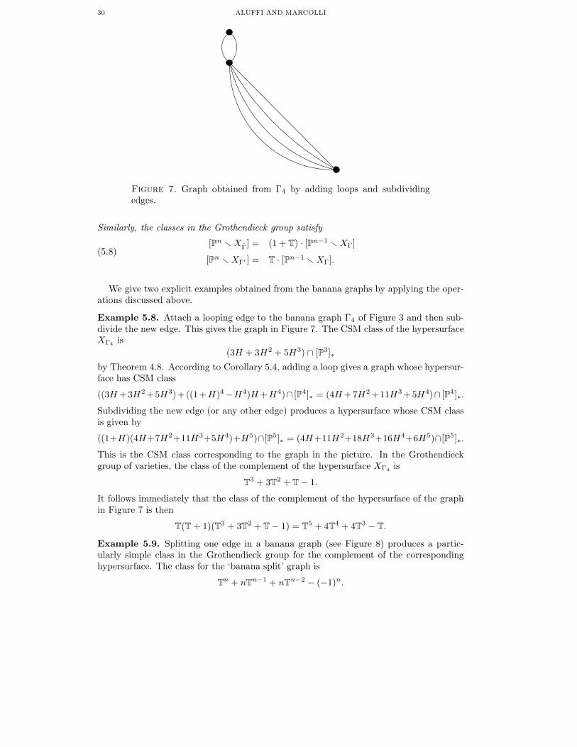
30 ALUFFI AND MARCOLLI
Figure 7. Graph obtained from Γ4 by adding loops and subdividingedges.
Similarly, the classes in the Grothendieck group satisfy
(5.8)[Pn r XΓ] = (1 + T) · [Pn−1 r XΓ]
[Pn r XΓ′ ] = T · [Pn−1 r XΓ].
We give two explicit examples obtained from the banana graphs by applying the oper-ations discussed above.
Example 5.8. Attach a looping edge to the banana graph Γ4 of Figure 3 and then sub-divide the new edge. This gives the graph in Figure 7. The CSM class of the hypersurfaceXΓ4
is
(3H + 3H2 + 5H3) ∩ [P3]∗
by Theorem 4.8. According to Corollary 5.4, adding a loop gives a graph whose hypersur-face has CSM class
((3H +3H2 +5H3)+((1+H)4−H4)H +H4)∩ [P4]∗ = (4H +7H2 +11H3 +5H4)∩ [P4]∗.
Subdividing the new edge (or any other edge) produces a hypersurface whose CSM classis given by
((1+H)(4H+7H2+11H3+5H4)+H5)∩[P5]∗ = (4H+11H2+18H3+16H4+6H5)∩[P5]∗.
This is the CSM class corresponding to the graph in the picture. In the Grothendieckgroup of varieties, the class of the complement of the hypersurface XΓ4
is
T3 + 3T2 + T − 1.
It follows immediately that the class of the complement of the hypersurface of the graphin Figure 7 is then
T(T + 1)(T3 + 3T2 + T − 1) = T5 + 4T4 + 4T3 − T.
Example 5.9. Splitting one edge in a banana graph (see Figure 8) produces a partic-ularly simple class in the Grothendieck group for the complement of the correspondinghypersurface. The class for the ‘banana split’ graph is
Tn + nTn−1 + nTn−2 − (−1)n.

BANANA MOTIVES 31
Figure 8. Banana split graph.
6. Banana graphs in Noncommutative QFT
Recently there has been growing interest in investigating the renormalization propertiesand the perturbative theory for certain quantum field theories on noncommutative space-times. These arise, for instance, as effective limits of string theory [16], [31]. In particular,in dimension D = 4, when the underlying R4 is made noncommutative by deformation toR4
θ with the Moyal product, it is known that the φ4 theory behaves in a very interestingway. In particular, the Grosse–Wulkenhaar model was proved to be renormalizable to allorders in perturbation theory (for an overview see [21]). We do not recall here the mainaspects of noncommutative field theory, as they are beyond the main purpose of this paper,but we mention the fact, which is very relevant to us, that a parametric representation forthe Feynman integrals exists also in the noncommutative setting (cf. [22], [32]). When theunderlying spacetime becomes noncommutative, the usual Feynman graphs are replacedby ribbon graphs, which account for the fact that, in this case, in the Feynman rulesthe contribution of each vertex depends on the cyclic ordering of the edges, cf. [21]. Forexample, in the ordinary commutative case, among the banana graphs Γn we consider inthis paper the only ones that can appear as Feynman graphs of the φ4 theory are the oneloop case (with two external edges at each vertex), the two loop case (with one externaledge at each vertex) and the three loop case as a vacuum bubble. Excluding the vacuumbubble because of the presence of the polynomial PΓ(t), we see that the effect of makingthe underlying spacetime noncommutative turns the remaining two graphs into the graphsof Figure 9. Notice how the two loop ribbon graph now has two distinct versions, only oneof which is a planar graph. The usual Kirchhoff polynomial ΨΓ(t) of the Feynman graph,as well as the polynomial PΓ(t, p), are replaced by new polynomials involving pairs ofspanning trees, one in the graph itself and one in another associated graph which is a dualgraph in the planar case and that is obtained from an embedding of the ribbon graph ona Riemann surface in the more general case. Unlike the commutative case, these polyno-mials are no longer homogeneous, hence the corresponding graph hypersurface only makessense as an affine hypersurface. The relation of the hypersurface for the noncommutativecase and the one of the original commutative case (also viewed as an affine hypersurface)is given by the following statement.
Proposition 6.1. Let Γ be a ribbon graph in the noncommutative φ4-theory that cor-responds in the ordinary φ4-theory to a graph Γ with n internal edges. Then instead ofa single graph hypersurface XΓ one has a one-parameter family of affine hypersurfacesXΓ,s ⊂ An, where the parameter s ∈ R+ depends upon the deformation parameter θ of
the noncommutative R4θ and on the parameter Ω of the harmonic oscillator term in the
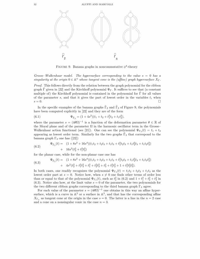
32 ALUFFI AND MARCOLLI
Γ Γ2 3
∼ ∼
Figure 9. Banana graphs in noncommutative φ4-theory
Grosse–Wulkenhaar model. The hypersurface corresponding to the value s = 0 has asingularity at the origin 0 ∈ An whose tangent cone is the (affine) graph hypersurface XΓ.
Proof. This follows directly from the relation between the graph polynomial for the ribbongraph Γ given in [22] and the Kirchhoff polynomial ΨΓ. It suffices to see that (a constant
multiple of) the Kirchhoff polynomial is contained in the polynomial for Γ for all valuesof the parameter s, and that it gives the part of lowest order in the variables ti whens = 0.
In the specific examples of the banana graphs Γ2 and Γ3 of Figure 9, the polynomialshave been computed explicitly in [22] and they are of the form
(6.1) ΨΓ2= (1 + 4s2)(t1 + t2 + t21t2 + t1t
22),
where the parameter s = (4θΩ)−1 is a function of the deformation parameter θ ∈ R ofthe Moyal plane and of the parameter Ω in the harmonic oscillator term in the Grosse–Wulkenhaar action functional (see [21]). One can see the polynomial ΨΓ2
(t) = t1 + t2appearing as lowest order term. Similarly for the two graphs Γ3 that correspond to thebanana graph Γ3 one has ([22])
(6.2)ΨΓ3
(t) = (1 + 8s2 + 16s4)(t1t2 + t2t3 + t1t3 + t21t2t3 + t1t22t3 + t1t2t
23)
+ 16s2(t22 + t21t23)
for the planar case, while for the non-planar case one has
(6.3)ΨΓ3
(t) = (1 + 8s2 + 16s4)(t1t2 + t2t3 + t1t3 + t21t2t3 + t1t22t3 + t1t2t
23)
+ 4s2(t22 + t21t23 + t21 + t22t
23 + t23 + t21t
22 + 1 + t21t
22t
23).
In both cases, one readily recognizes the polynomial ΨΓ3(t) = t1t2 + t2t3 + t1t3 as the
lowest order part at s = 0. Notice how, when s 6= 0 one finds other terms of order lessthan or equal to that of the polynomial ΨΓ3
(t), such as t22 in (6.2) and 1 + t21 + t22 + t23 in(6.3). Notice also how, at the limit value s = 0 of the parameter, the two polynomials forthe two different ribbon graphs corresponding to the third banana graph Γ3 agree.
For each value of the parameter s = (4θΩ)−1 one obtains in this way an affine hyper-surface, which is a curve in A2 or a surface in A3, and that has the corresponding affineXΓn
as tangent cone at the origin in the case s = 0. The latter is a line in the n = 2 caseand a cone on a nonsingular conic in the case n = 3.

BANANA MOTIVES 33
As a further example of why it is useful to compute invariants such as the CSM classesfor the graph hypersurfaces, we show that the CSM class of the hypersurface defined bythe polynomial (6.2) detects the special values of the deformation parameter s = (4θΩ)−1
where the hypersurface XΓ3becomes more singular and gives a quantitative estimate of
the amount by which the singularities change.The CSM class is naturally defined for projective varieties. In the case of an affine
hypersurface defined by a non-homogeneous equation, one can choose to compactify it inprojective space by adding an extra variable and making the equation homogeneous andthen computing the CSM class of the corresponding projective hypersurface. However, indoing so one should be aware of the fact that the CSM class of an affine variety, defined bychoosing an embedding in a larger compact ambient variety, depends on the choice of theembedding. An intrinsic definition of CSM classes for non-compact varieties which doesnot depend on the embedding was given in [2], [1]. However, for our purposes here it sufficesto take the simpler viewpoint of making the equation homogeneous and then computingCSM classes. If we adopt this procedure, then by numerical calculations performed withthe Macaulay2 program of [4] we obtain the following result.
Proposition 6.2. Let XΓ3⊂ P3 denote the affine surface defined by the equation (6.2)
and let XΓ3⊂ P3 be the hypersurface obtained by making the equation (6.2) homogeneous.
For general values of the parameter s = (4θΩ)−1 the CSM class is given by
(6.4) c(XΓ3) = 14H3 + 4H.
For the special value s = 1/2 of the parameter, the CSM class becomes of the form
(6.5) c(XΓ3)|s=1/2 = 5H3 + 5H2 + 4H,
while in the limit s → 0 one has
(6.6) c(XΓ3)|s=0 = 11H3 + 4H.
It is also interesting to notice that, when we consider the second equation (6.3) forthe non-planar ribbon graph associated to the third banana graph Γ3, we see an examplewhere the graph hypersurfaces of the non-planar graphs of noncommutative field theory nolonger satisfy the positivity property of Conjecture 1.5 that appears to hold for the graphhypersurfaces of the commutative field theories. In fact, as in the case of the equation forthe planar graph (6.2), we now find the following result.
Proposition 6.3. Let XΓ3⊂ P3 denote the affine surface defined by the equation (6.3)
and let XΓ3⊂ P3 be the hypersurface obtained by making the equation (6.3) homogeneous.
For general values of the parameter s = (4θΩ)−1 the CSM class is given by
(6.7) c(XΓ3) = 33H3 − 9H2 + 6H.
The special case s = 1/2 is given by
(6.8) c(XΓ3)|s=1/2 = 9H3 − 3H2 + 6H
Notice that, in the case of ordinary Feynman graphs of commutative scalar field theories,all the examples where the CSM classes of the corresponding hypersurfaces have beencomputed explicitly (either theoretically or numerically) are planar graphs. Although itseems unlikely that planarity will play a role in the conjectured positivity of the coefficientsof the CSM classes in the ordinary case, the example above showing that CSM classes ofgraph hypersurfaces of non-planar ribbon graphs in noncommutative field theories canhave negative coefficients makes it more interesting to check the case of non-planar graphsin the ordinary case as well. It is well known that, for an ordinary graph to be non-planar,it has to contain a copy of either the complete graph K5 on five vertices or the complete

34 ALUFFI AND MARCOLLI
bipartite graph K3,3 on six vertices. Either one of these graphs corresponds to a graphpolynomial that is currently beyond the reach of the available Macaulay2 routine anda theoretical argument that provides a more direct approach to the computation of thecorresponding CSM class does not seem to be easily available. It remains an interestingquestion to compute these CSM classes, especially in view of the fact that the originalcomputations of [15] of Feynman integrals of graphs appear to indicate that the non-planarity of the graph is somehow related to the presence of more interesting periods (e.g.multiple as opposed to simple zeta values). It would be interesting to see whether it alsohas an effect on invariants such as the CSM class.
References
[1] P. Aluffi, Classes de Chern des varietes singulieres, revisitees. C. R. Math. Acad. Sci. Paris 342(2006), no. 6, 405–410.
[2] P. Aluffi, Limits of Chow groups, and a new construction of Chern-Schwartz-MacPherson
classes. Pure Appl. Math. Q. 2 (2006), no. 4, 915–941.[3] P. Aluffi, Modification systems and integration in their Chow groups. Selecta Math. (N.S.) 11
(2005), no. 2, 155–202.[4] P. Aluffi, Computing characteristic classes of projective schemes. J. Symbolic Comput. 35 (2003),
no. 1, 3–19.[5] P. Aluffi, Chern classes for singular hypersurfaces. Trans. Amer. Math. Soc. 351 (1999), no. 10,
3989–4026.
[6] P. Aluffi, MacPherson’s and Fulton’s Chern classes of hypersurfaces, Internat. Math. Res. No-tices, Vol.11 (1994) 455–465.
[7] P. Aluffi, L.C. Mihalcea, Chern classes of Schubert cells and varieties, arXiv:math/0607752. Toappear in Journal of Algebraic Geometry.
[8] P. Belkale, P. Brosnan, Matroids, motives, and a conjecture of Kontsevich, Duke Math. Journal,Vol.116 (2003) 147–188.
[9] J. Bjorken, S. Drell, Relativistic Quantum Mechanics, McGraw-Hill, 1964, and Relativistic Quan-
tum Fields, McGraw-Hill, 1965.[10] S. Bloch, Motives associated to graphs, Japan J. Math., Vol.2 (2007) 165–196.[11] S. Bloch, E. Esnault, D. Kreimer, On motives associated to graph polynomials, Commun. Math.
Phys., Vol.267 (2006) 181–225.[12] S. Bloch, D. Kreimer, Mixed Hodge structures and renormalization in physics, arXiv:0804.4399.[13] J.-P. Brasselet, D. Lehmann, J. Seade, T. Suwa, Milnor classes of local complete intersections,
Trans. Amer. Math. Soc., Vol.354(2002) N.4, 1351–1371.[14] J.P. Brasselet, M.H. Schwartz, Sur les classes de Chern d’un ensemble analytique complexe, in
“The Euler-Poincare characteristic”, Asterisque, Vol.83, pp.93–147, Soc. Math. France, 1981.[15] D. Broadhurst, D. Kreimer, Association of multiple zeta values with positive knots via Feynman
diagrams up to 9 loops, Phys. Lett. B, Vol.393 (1997) 403–412.[16] A.Connes, M.Douglas, A.Schwarz, Noncommutative geometry and matrix theory: compactifica-
tion on tori. JHEP 9802 (1998) 3–43.[17] A. Connes, D. Kreimer, Renormalization in quantum field theory and the Riemann–Hilbert
problem I. The Hopf algebra structure of graphs and the main theorem, Comm. Math. Phys.,Vol.210 (2000) 249–273.
[18] W. Fulton, Intersection theory. Ergebnisse der Mathematik und ihrer Grenzgebiete (3) 2.Springer-Verlag, 1984. xi+470 pp.
[19] H. Gillet, C.Soule, Descent, motives and K-theory. J. Reine Angew. Math. 478 (1996), 127–176.[20] D.R. Grayson, M.E. Stillman, Macaulay 2, a software system for research in algebraic geometry,
available at http://www.math.uiuc.edu/Macaulay2/
[21] H. Grosse, R. Wulkenhaar, Renormalization of noncommutative quantum field theory, in “Aninvitation to Noncommutative Geometry” pp.129–168, World Scientific, 2008.
[22] R. Gurau, V. Rivasseau, Parametric Representation of Noncommutative Field Theory, Commun.Math. Phys. Vol. 272 (2007) N.3, 811–835
[23] C. Itzykson, J.B. Zuber, Quantum Field Theory, Dover Publications, 2006.[24] M. Kwiecinski, Formule du produit pour les classes caracteristiques de Chern-Schwartz-
MacPherson et homologie d’intersection, C. R. Acad. Sci. Paris Ser. I Math., 314(1992) N.8,625–628.

BANANA MOTIVES 35
[25] R.D. MacPherson, Chern classes for singular algebraic varieties. Ann. of Math. (2) 100 (1974),423–432.
[26] M. Marcolli, Motivic renormalization and singularities, arXiv:0804.4824.[27] N. Nakanishi Graph Theory and Feynman Integrals. Gordon and Breach, 1971.[28] A. Parusinski, A generalization of the Milnor number, Math. Ann. Vol.281 (1988) N.2, 247–254.[29] M.H. Schwartz, Classes caracteristiques definies par une stratification d’une variete analytique
complexe. I. C. R. Acad. Sci. Paris Vol.260 (1965) 3262–3264.[30] M.H. Schwartz, Classes caracteristiques definies par une stratification d’une variete analytique
complexe, C. R. Acad. Sci. Paris, Vol.260 (1965) 3535–3537.[31] N. Seiberg, E. Witten, String theory and noncommutative geometry, JHEP 9909 (1999) 32–131.[32] A. Tanasa, Overview of the parametric representation of renormalizable non-commutative field
theory, arXiv:0709.2270.
Department of Mathematics, Florida State University, Tallahassee, FL 32306, USA
E-mail address: [email protected]
E-mail address: [email protected]
Max–Planck Institut fur Mathematik, Vivatsgasse 7, Bonn, D 53111, Germany
E-mail address: [email protected]
E-mail address: [email protected]