fertility and female labor force participation: evidence...

Fertility and Female Labor Force Participation: Evidence from

the One-Child Policy in China

Hui Wang∗

[email protected]

December 3, 2014

Abstract

Unlike in the United States where fertility is found to be negatively correlated with femalelabor force participation, China has witnessed a decrease in both fertility and female laborforce participation since the 1980s. Does fertility play a different role in female labor forceparticipation in China than in the U.S.? To answer this question, this paper exploits plausiblyexogenous variations in fertility created by the affirmative One-Child Policy in China to estimatethe effect of having two or more children on the mother’s labor force participation. Using a largedata set from the 1990 Population Census, I find that OLS underestimates the negative effectsof fertility, and 2SLS estimates imply that conditional on having one child, additional childrendecreases mother’s female labor force participation by 8-15 percentage points in rural China.Recently, there has been a call for relaxation of the One-Child Policy in China, our finding hereprovides a perspective for the potential effects of such policy relaxations on female labor supply.

Keywords: Fertility; Female Labor Force Participation; the One-Child Policy; China

JEL Classification: J13; J22; O15

∗Department of Economics, Department of Agricultural, Food and Resource Economics, Michigan State University.The author is grateful to Todd Elder, Songqing Jin, Leah Lakdawala, Steven Haider, Scott Imberman, Jeffrey M.Wooldridge, James J. Heckman, Xiaobao Zhang, Karen Eggleston and all participants in Applied Economics Seminarat Michigan State University, and China Meeting of Econometric Society for helpful comments. The author claimsresponsibility for the remaining shortcomings of the paper.

1

1 Introduction

Inspired in part by a contemporaneous increase in female labor force participation and a decrease in

fertility in the U.S. (Figure 1), many economists have investigated the effects of number of children on

mother’s labor supply (Klerman (1999), Angrist and Evans (1998), and Bailey (2006) etc.). Angrist

and Evans (1998) and many others find negative effects of fertility on female labor force participation

in the U.S.1 On the other side of the world, China has implemented the One-Child Policy since 1979

aiming at curbing its fast population growth; however, surprisingly, with fewer children, it appears

that women in China participate less in the labor force (Figure 2). In this study, I examine the

effects of fertility on female labor force participation in rural China.2 Are the effects of fertility in

China the same as found in the U.S., or are they opposite, as suggested by the information found

in Figure 1 and Figure 2? This paper can help us answer this question.

[Insert Figure 1 Here.]


Empirically analyzing the effect of fertility on female labor force participation is challenging

due to the endogeneity of fertility decisions with respect to labor supply. Willis (1974) shows that

female labor force participation and fertility are always jointly determined. For example, if omitted

variables such as women’s preferences for work are negatively correlated with their preferences for

having more children, or if the time and effort spent on work discourages fertility (generating reverse

causality), then the estimates of the effect of number of children on female labor supply would be

biased downward. The bias could also go in the opposite direction; for example, some have found

that fertility in developing countries is determined through a collective bargaining process at the

household level and household members with more bargaining power have more influence on the

total number of children (Rasul, 2008). In addition, men are generally found to prefer more children

than women in developing countries (Mason and Taj, 1987). If women with less bargaining power

are forced to work as well as have more children, then naive OLS regressions will underestimate the

negative impact of children on mother’s labor force participation.

To address this endogeneity problem, economists have exploited various sources of exogenous

variation in family size such as twinning (Rosenzweig and Wolpin (1980), Jacobsen et al. (1999)),

1A negative correlation between fertility and female labor force participation has been found both over time andcross countries (Aguero and Marks, 2011).

2I exploit two sources of variation in fertility that arise due to the One-Child Policy: gender at first birth andethnicity. Since gender at first birth is relevant for the implementation of the OCP only in rural areas (Qian, 2009), Ifocus on rural China for this study. Moreover since the penalties imposed on those who exceed their quota in urbanareas may involve job loss, the OCP may directly affect labor force participation in these areas and thus I excludeurban areas from this analysis.

2

sex composition of the first two births (Angrist and Evans, 1998),3 state-level access to contraception

(Bailey, 2006), and state-level abortion laws (Klerman (1999), Levine et al. (1999), and Angrist and

Evans (2000)). All of these U.S.-based studies found solid evidence of a negative effect of fertility

on female labor supply.

In contrast, studies based on developing countries show mixed results on the effect of fertility

on maternal labor supply. Using data from a randomized social experiment in Matlab, Bangladesh,

Schultz (2009) found a negative effect for family planning programs (which lead to lower fertility) on

the likelihood of “work for pay” for women. Using son-preference4 as an instrument, Ebenstein (2009)

indentified negative effects of fertility on maternal labor force participation in Taiwan. Based on data

from Demographic and Health Surveys covering 59 developing countries (excluding China), using

son-preference, the sex composition of first and second born children, and twinning as instruments,

Porter and King (2010) reported that while in many developing countries women are less likely to

work when they have more children, in some countries, mothers with more children are more likely

to work due to reasons such as the financial costs of raising more children. Combining data from

Demographic and Health Surveys with abortion legislation documents in each country, Bloom et al.

(2009) confirmed these mixed results on the effects of fertility. In a cross-country study, Aguero and

Marks (2011) analyzed 26 low- and middle-income countries, and using infertility as an instrument

for family size. They found that number of children has no effect on labor force participation and

work intensity.

I am aware of only one existing study on the impact of fertility on female labor supply in the

context of China. Based on information from 1,315 women from the China Health and Nutrition

Survey conducted in 1993, Lee (2002) used the sex of the first child as an instrument5 and found

no significant effects of fertility on rural female labor supply in China.6 The main concern when

using son-preference as an instrument for total fertility is that the gender of the first-born child may

not satisfy the exclusion restriction condition, since previous work has shown that children’s gender

affects mothers’ labor supply directly (Cruces and Galiani, 2007).

In order to curb rapid population growth, the Chinese government has implemented the One-

Child Policy (OCP) since 1979, possibly the largest social experiment in human history. Under this

3They found parents of two children of the same sex have higher probability of having a third birth than parentsof one boy and one girl.

4In east Asian countries, families are found to have strong preference for male children. In particular, families withtwo girls have higher probability to have third child.

5With strong son-preference, the parents in China are found to have more children when they have no sons yet(Ebenstein, 2009).

6Lee (2002) also attempted to use the One-Child Policy, in particular, “local family planning rules” as instruments,but he admitted this instrument was potentially endogenous. I discuss this in more detail in Section 3.3.

3

policy, a married couple can have only one child in most areas of the country. However, there are

several important exceptions. The first is that the OCP was not applied to non-Han Chinese until

1988. The second exception arose when, in some areas, it was observed that the OCP was associated

with female infanticide, forced abortion and forced sterilization. To prevent these extreme cases, 19

provinces adopted the “1-boy-2-girl” rule in 1984, which stated that rural couples in these provinces

were allowed to have a second child if the first child was a girl (Qian, 2009).

In this paper, I exploit two sources of exogenous variation in fertility generated by the One-Child

Policy in China. More specifically, I use the differences in the policy’s implementation between the

Han and non-Han Chinese, as well as between rural couples with first-born girls and those with first-

born boys in the 19 provinces that adopted the “1-boy-2-girl” rule to instrument for the likelihood a

woman has two or more children. Thus the identification comes from variation in fertility generated

by the OCP across cohorts of women (those affected and not affected by the policy during their fertile

years), ethnicities (Han and non-Han), and families based on the gender of their first-born children.

Assuming that without the variation in the OCP the differences between women in the unaffected

(old) and affected (young) cohorts would be the same for the Han and non-Han, the differences-

in-differences estimates based on ethnicity will capture the exogenous variation of fertility due to

the variation in the OCP. Similarly, under the assumption that the differences between women in

different age cohorts would be the same for women with either first-born boys or first-born girls

without the variation in the OCP, DID estimates based on gender of first birth can capture the

exogenous variations of fertility generated by the OCP. Using a large random sample from the 1990

China Population Census, the results show that OLS regressions underestimate the discouraging

effects of children on female labor force participation. After accounting for the endogeneity of

fertility, the likelihood of labor force participation for mothers with two or more children is 8 to 15

percentage points lower than for mothers with only one child in rural China in 1990.

This paper makes several contributions. First, it aims to fill the knowledge gap on effects of

fertility on female labor supply in China, the most populous country in the world with a controversial

population control. Along with the substantial drop in fertility experienced over the last 30 years,

China witnessed a decline in female labor force participation, raising doubts as to whether the

observed negative relationship between fertility and female labor force participation observed in

developed countries extends to the developing country setting. By identifying the causal effects of

fertility on female labor force participation in China, this research can enrich our understanding of

the effects of fertility on female labor supply.

Second, the majority of past research focused on the effects of an additional child for the select

4

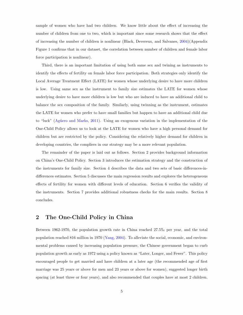
sample of women who have had two children. We know little about the effect of increasing the

number of children from one to two, which is important since some research shows that the effect

of increasing the number of children is nonlinear (Black, Devereux, and Salvanes, 2004)(Appendix

Figure 1 confirms that in our dataset, the correlation between number of children and female labor

force participation is nonlinear).

Third, there is an important limitation of using both same sex and twining as instruments to

identify the effects of fertility on female labor force participation. Both strategies only identify the

Local Average Treatment Effect (LATE) for women whose underlying desire to have more children

is low. Using same sex as the instrument to family size estimates the LATE for women whose

underlying desire to have more children is low but who are induced to have an additional child to

balance the sex composition of the family. Similarly, using twinning as the instrument, estimates

the LATE for women who prefer to have small families but happen to have an additional child due

to “luck” (Aguero and Marks, 2011). Using an exogenous variation in the implementation of the

One-Child Policy allows us to look at the LATE for women who have a high personal demand for

children but are restricted by the policy. Considering the relatively higher demand for children in

developing countries, the compliers in our strategy may be a more relevant population.

The remainder of the paper is laid out as follows. Section 2 provides background information

on China’s One-Child Policy. Section 3 introduces the estimation strategy and the construction of

the instruments for family size. Section 4 describes the data and two sets of basic differences-in-

differences estimates. Section 5 discusses the main regression results and explores the heterogeneous

effects of fertility for women with different levels of education. Section 6 verifies the validity of

the instruments. Section 7 provides additional robustness checks for the main results. Section 8

concludes.

2 The One-Child Policy in China

Between 1962-1970, the population growth rate in China reached 27.5h per year, and the total

population reached 816 million in 1970 (Yang, 2004). To alleviate the social, economic, and environ-

mental problems caused by increasing population pressure, the Chinese government began to curb

population growth as early as 1972 using a policy known as “Later, Longer, and Fewer”. This policy

encouraged people to get married and have children at a later age (the recommended age of first

marriage was 25 years or above for men and 23 years or above for women), suggested longer birth

spacing (at least three or four years), and also recommended that couples have at most 2 children.

5

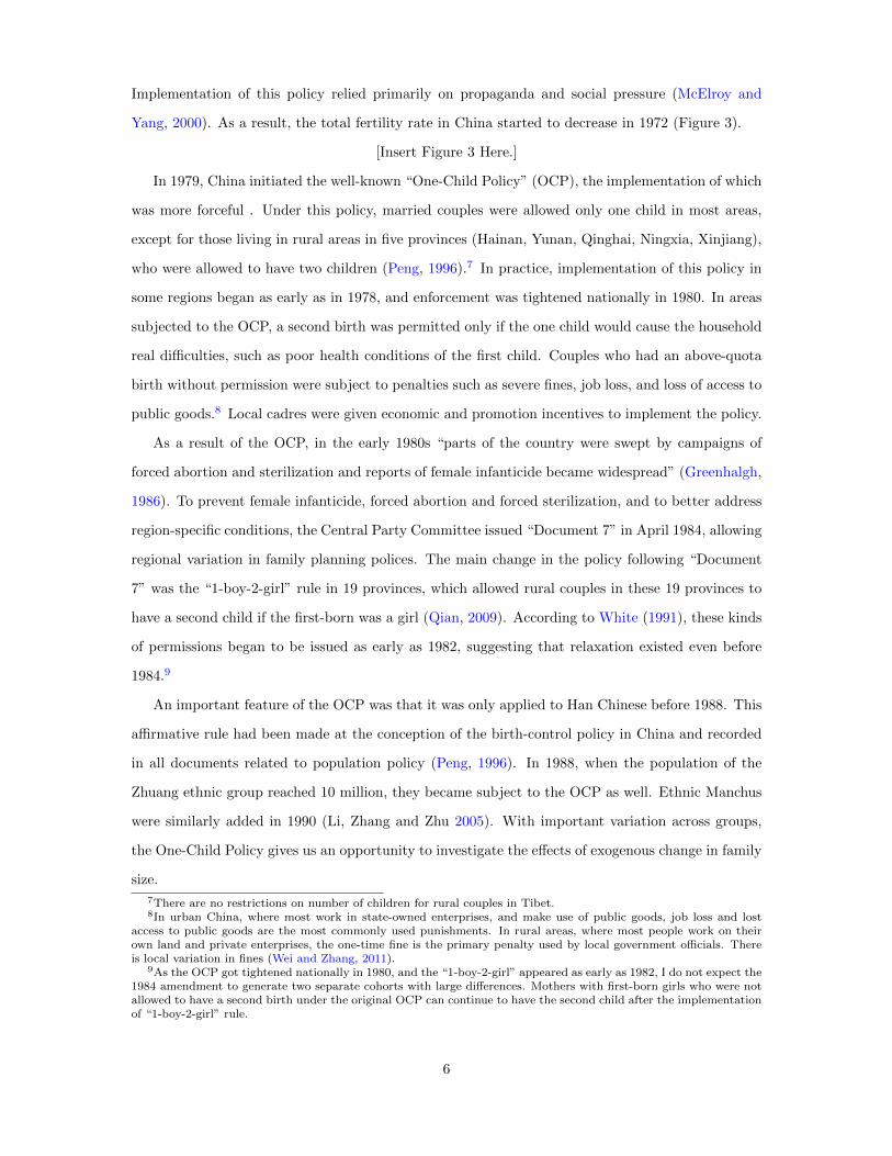
Implementation of this policy relied primarily on propaganda and social pressure (McElroy and

Yang, 2000). As a result, the total fertility rate in China started to decrease in 1972 (Figure 3).


In 1979, China initiated the well-known “One-Child Policy” (OCP), the implementation of which

was more forceful . Under this policy, married couples were allowed only one child in most areas,

except for those living in rural areas in five provinces (Hainan, Yunan, Qinghai, Ningxia, Xinjiang),

who were allowed to have two children (Peng, 1996).7 In practice, implementation of this policy in

some regions began as early as in 1978, and enforcement was tightened nationally in 1980. In areas

subjected to the OCP, a second birth was permitted only if the one child would cause the household

real difficulties, such as poor health conditions of the first child. Couples who had an above-quota

birth without permission were subject to penalties such as severe fines, job loss, and loss of access to

public goods.8 Local cadres were given economic and promotion incentives to implement the policy.

As a result of the OCP, in the early 1980s “parts of the country were swept by campaigns of

forced abortion and sterilization and reports of female infanticide became widespread” (Greenhalgh,

1986). To prevent female infanticide, forced abortion and forced sterilization, and to better address

region-specific conditions, the Central Party Committee issued “Document 7” in April 1984, allowing

regional variation in family planning polices. The main change in the policy following “Document

7” was the “1-boy-2-girl” rule in 19 provinces, which allowed rural couples in these 19 provinces to

have a second child if the first-born was a girl (Qian, 2009). According to White (1991), these kinds

of permissions began to be issued as early as 1982, suggesting that relaxation existed even before

1984.9

An important feature of the OCP was that it was only applied to Han Chinese before 1988. This

affirmative rule had been made at the conception of the birth-control policy in China and recorded

in all documents related to population policy (Peng, 1996). In 1988, when the population of the

Zhuang ethnic group reached 10 million, they became subject to the OCP as well. Ethnic Manchus

were similarly added in 1990 (Li, Zhang and Zhu 2005). With important variation across groups,

the One-Child Policy gives us an opportunity to investigate the effects of exogenous change in family

size.

7There are no restrictions on number of children for rural couples in Tibet.8In urban China, where most work in state-owned enterprises, and make use of public goods, job loss and lost

access to public goods are the most commonly used punishments. In rural areas, where most people work on theirown land and private enterprises, the one-time fine is the primary penalty used by local government officials. Thereis local variation in fines (Wei and Zhang, 2011).

9As the OCP got tightened nationally in 1980, and the “1-boy-2-girl” appeared as early as 1982, I do not expect the1984 amendment to generate two separate cohorts with large differences. Mothers with first-born girls who were notallowed to have a second birth under the original OCP can continue to have the second child after the implementationof “1-boy-2-girl” rule.

6

3 Estimation Strategy

Following the literature, the main regression model we are interested in can be written as:

LFPict = βkids2ict + X′ictδ + α1 + γt + ψc + εict (1)

where LFPict is the labor force participation indicator for woman i in county c, age cohort t. Follow

Maurer-Fazio, Hughes and Zhang (2005), LFPict = 1 if the woman had a job on the day of the

census or if she was unemployed but was coded as “waiting for work”. It would be ideal if we can

measure women supply in both extensive margin and intensive margin. However, with the limited

information provided in 1990 China Population Census, I focus only on the extensive margin in this

study. kids2ict is a dummy variable equal to 1 if the woman has two or more children;10 Xict is a

vector of woman i’s characteristics, including her age, age at first birth, ethnicity, gender of the first

child, and education levels for both her and her husband;11 γt is the age cohort fixed effect, and ψc

denotes the county fixed effect. We use the dummy variable kids2ict to measure fertility rather than

number of children, since our DID estimates only apply to the discrete change from one child to two

or more children. Angrist and Imbens (1995) indicates that the resulting estimated effects will be

bigger than the true average per-unit effect when the treatment variable is incorrectly parameterized

as binary, while the sign of the Average Causal Effect is still consistently estimated. As the effects

of children on female labor supply are likely to be non-linear (Appendix Figure 1), we take caution

in interpreting our estimates of the coefficient on kids2ict.

Women’s labor force participation may affect fertility decisions and there might be unobserved

factors (e.g. health) that affect LFPict and kids2ict simultaneously. For these reasons and others, we

believe that the condition cov (kids2ict, εict) = 0 does not hold. As a result, the OLS estimator of β is

not consistent. To address this endogeneity problem, I use two sets of differences-in-differences (DID)

strategies to construct exogenous variation in fertility, and then use this variation to instrument

kids2ict in Equation (1). The first DID strategy exploit the differences in the probability of having

two or more children between Han and non-Han Chinese, for women affected and unaffected by the

OCP; while the second strategy compares the differences between women with first-born girls and

women with first-born boys, for affected and unaffected cohorts.

10All women in our sample have at least one child; therefore, kids2ict = 0 means the woman has only one child.11Table 1 reports the definition of the key variables (dependent variables, covariates, and instruments).

7

3.1 DID using ethnicity

As described in Section 2, before 1988 only Han Chinese were subject to the strict One-Child Policy,

while non-Han couples were allowed to have two children. One attractive estimation strategy, there-

fore, is to use ethnicity to capture the exogenous variations in number of children. Unfortunately,

knowledge about China as well as summary statistics shown in Section 4 suggest that there are

many systematic differences between Han and non-Han Chinese. Therefore, one would worry that

ethnicity might directly affect women’s labor force participation decisions, and thus the exclusion

restriction will not hold if we use ethnicity alone as an instrument.

Using DID can help remove the first order differences between Han and non-Han Chinese. The

DID method can be simply expressed as (nonHan, After − Han, After) − (nonHan, Before −

Han, Before). Under the assumption that without the OCP, the difference in female labor force

participation between affected and unaffected cohorts would be the same for Han and non-Han

individuals, DID estimates will capture the exogenous variations of kids2ict due to the variation in

the OCP, which affects different ethnic groups differently.

Here, we use After to represent females restricted by the OCP, that is, the young cohorts in

our sample. Before denotes the cohort not constrained by the OCP, that is, the old cohorts who

probably had two or more children already before 1979/1980. Though the One-Child Policy was

announced in 1979, there is no simple distinction between exposed/treated and non-exposed/non-

treated individuals, as people choose their fertility timing differently. Appendix Figure 3a depicts

the cumulative distribution of age at second birth for the restricted provinces sample. It shows that

over 90% of women with two or more children gave birth to their second child before the age of 30.

Considering 1980 as the year that the OCP became nationally implemented, I assume that women

older than 30 in 1980 were relatively less-constrained by the OCP. The cutoff age of 30 in 1980 means

that the cutoff age is 40 in 1990. Thus, women older than 40 in the 1990 census will be regarded as

Before cohorts, while women age 40 or younger will be the After cohorts. In regressions, rather

than arbitrarily dividing the women into these two cohorts, I use age cohort dummies to allow

for the most flexibility in the effect of the OCP on fertility. Using DID to capture the exogenous

variation in fertility caused by exogenous variation in policy change is fundamentally equivalent to

using interaction terms. Hence, the first stage regression of kids2ict on the interaction terms will

have the following form:

kids2ict =

44∑l=16

(nonHanict · dl) ρl + X′ictκ+ α2 + dt + θc + uict (2)

8

where dl, l = 16 to 44 are age dummies from 16 to 44 years of age.12

3.2 DID using gender of first-birth

In 1984, to prevent female infanticide, forced abortion and forced sterilization, an amendment to

the original OCP was implemented in 19 provinces in 1984. Under the amendment, a rural couple is

allowed to have a second child if their first child is a girl, also known as the “1-boy-2-girl” rule. This

amendment provides us with another DID strategy to construct the exogenous variation in fertility.

Cruces and Galiani (2007) find that the gender of children directly affects women’s labor supply

in Mexico and Argentina. This might be true in Asia, especially in China, as well. In rural China,

where the preference for sons is strong, boys are valued more highly than girls. It might be expected

that the mothers with sons would spend more time on childcare than mothers with daughters. In

this case, the gender of children will directly affect a mother’s labor supply. However, we can remove

the direct effect of first-born gender on female labor supply using DID. The DID method can be

expressed as (First-Born Girl, After − First-Born Boy, After) − (First-Born Girl, Before −

First-Born Boy, Before). As above, After represents the treated or young cohort, while Before

denotes the control or old cohort. In all regressions, I include age cohort dummies. The key

assumption in this DID strategy is that without the variation in the OCP, the difference in female

labor force participation decision between treatment and control cohorts would be the same for

women whose first child is a son and those whose first child is a daughter. My first stage regression

using interaction terms of age cohorts and gender of first birth is thus:

kids2ict =

44∑l=22

(First-Born Girlict · dl)φl + X′ictµ+ α3 + dt + πc + vict (3)

where dl, l = 16 to 44 are age dummies from 16 to 44 years of age.

3.3 Other research using the OCP to construct instruments for fertility

Although there exists only one study exploring the effects of fertility on female labor force partic-

ipation in China, the strategy of using the variation in implementation of the OCP to instrument

for fertility has been widely adopted in several studies exploring the effects of fertility on other

outcomes in China. Short and Zhai (1998) show that in practice, the implementation of the OCP

varied geographically. Some of the research tries to exploit these spatial variation in the imple-

mentation of the One-Child Policy. For example, in her study of the effects of number of children

12Reasons for using these cohorts are discussed in Section 4.

9

on school enrollment of the first-born, Qian (2009) used the implementation of the “1-boy-2-girl”

rule at county level interacted with year and gender of first birth as instruments for number of

children. However, when Lee (2002) tries to use local family planning rules as instruments for two

or more children, he finds that the implementation of the “1-boy-2-girl” rules at the county level is

significantly correlated with community location and infrastructure. Communities located far away

from cities and/or with poor infrastructure are more likely to implement this rule. Therefore, these

local rules may be endogenous to local labor market, so we do not use them as an instrument in our

study.13

In other related studies, researchers use the year of the first birth to instrument for fertility. To

estimate the effect of number of children on elderly parents’ health, Islam and Smyth (2010) use the

interaction terms of a rural/urban indicator and three period dummies corresponding to the year

of the first birth. When investigating the effects of fertility on parent’s saving behavior, Banerjee,

Meng and Qian (2010) use a dummy for whether the first birth was before 1972 to capture the effect

of the “Later, Longer, Fewer” policy on the number of children. The potential problem with this IV

strategy is that the year of the first birth for a given woman is determined by the couple, and thus

can be endogenous.14

To examine the impact of family size on mothers’ health, Wu and Li (2011) use the interactions

of a non-Han dummy and a measure of time exposure to the OCP. This strategy is similar to the

one implemented in this paper. In particular, they assume that the effects of exposure to the policy

is linear15 and they choose an arbitrary year when the policy starts to take effect. Using our data,

I can show that allowing for more flexible effects of the OCP on each age cohorts generates similar

but different results from using their strategy (Appendix Table 1 indicate that using identification

strategy in Wu and Li (2011) generates less precise estimate for the effect of children on female LFP,

and Appendix Table 2 shows the regression results when using a modified strategy based on gender

of the first-born, with the confidence interval for β2SLS as wide as (-1.70, -0.019), surpassing the

13Lee (2002) mainly exploited three local rules, i.e., under three different scenarios, whether a community allowsa couple to have a second child or not. The three scenarios are: 1) the first born child is a girl; 2) both husbandand wife are from a one-child family; 3) one parent has “dangerous” job. Only first rule satisfies “relevance” as aninstrument. However, when using both the first rule and gender of first child as instruments, Lee finds different resultsfrom using gender of first child as the only instrument. As a result, over-identification test is rejected. Assuminggender of first-birth is exogenous, Lee claimed that the implementation of the “first rule” at the county level is not avalid IV. He also tried to put “first rule” directly in OLS regression of number of children, and generated a significantlynegative coefficients. In addition, he found that county-level “first rule” implementation is significantly correlated withcommunity location and infrastructure. Communities located far away from cities and/or with poor infrastructuresare more likely to implement this rule. Put all these together, he claimed local “1-boy-2-girl” rule at the county levelis endogenous to the local labor market.

14In the sample we use in this paper, IV results are very different when using year of first birth dummies insteadof age cohort dummies, even after controlling for the mother’s age at first birth. Regression results available uponrequests.

15Figure 5a shows this is not true, especially when including very young age cohorts.

10

limit of -1).

Our DID method using ethnicity is motivated by a study by Li et al. (2005). In order to measure

the effect of the OCP on fertility,16 Li et al. (2005) use the interactions of a mother’s birth cohorts

and a Han dummy to identify the exogenous variation in number of children due to the OCP. Their

robustness tests show that changes in other household decisions, such as marriage and the decisions

whether to have any children, are not systematically different between Han and non-Han people

during this period.

4 Data and Descriptive Statistics

The data used in this paper comes from a 1% sample of the 1990 China Population Census, the fourth

census in China. For studies on fertility and labor supply, census data has the distinct advantages

of large sample size and national representation. For this study, which relies on exposure to the

One-Child Policy, the 1990 Census has three particular advantages. First, if we use the 2000 census

to do the analysis, our control cohorts would be 50 years old at the time of the survey. Though 55

is the official retirement age for women in China, many women retire as early as 50 (Maurer-Fazio

et al., 2011). As a result, the decision of whether or not to work and how it relates to fertility is not

likely to be relevant for the control group. 17 Second, though there was a 1982 Census, some aspects

of the OCP and important exceptions (including the 1-boy-2-girl rule) were not implemented until

after 1982. Third, before the 1990s, the household mobility in China was almost zero due to the

very strict household registration (Hukou) system. This helps to reduce the concern that families

endogenously migrate in response to the OCP.

The 1990 China Population Census contains limited but essential information at the household

and the individual level, including: age, sex, ethnicity, relationship to the household head, geographic

location (at county level), education, employment status, marital status, and childbearing status.

Detailed information about the census can be found in Wang (2000). Only three labor supply related

questions are included in 1990 censuses: employment status, industry and occupation. I follow

Maurer-Fazio et al. (2005) to define my dependent variable, the female labor force participation

(LFP ). LFPict = 1 if a woman has a job on the day of the census or if she is unemployed but is

coded as “waiting to be employed”.18 Two types of childbearing questions were asked for women

16They use DID directly, rather than apply it as IV.17The effects of number of children on female LFP depend heavily on the age group. Angrist and Evans (1998)

shows that the negative effects of children on female labor supply will disappear for children age 13 or older.18For individuals aged 15 and above, 1990 Population Census first asked their industries and occupations. For those

who did not answer these two, they were asked questions further about their non-employment status, with choiceslisted as: 1. currently enrolled; 2. student; 3. housework; 4. waiting for schooling; 5. waiting to be employed; 6.

11

aged 15 to 64: the birth history in the previous year and the number of sons and daughters ever born

and the number of surviving. No other retrospective fertility information is collected in the 1990

Census. Similar to Angrist and Evans (1998), I match children to mothers within the households to

get detailed information for the children.

The differences between urban and rural areas in China are huge. As noted in Section 2, the

implementation of the One-Child Policy in urban areas may have direct impacts on female labor

demand (as the most commonly-used penalty for above-quota birth is the job loss), which might

confound the 2SLS estimates. Therefore, this paper will focus on the effects of family size on

female labor force participation in rural China only. I include the households that are registered as

agricultural households and also resided in the countryside in the study sample.19 In order to link

the children to their parents, the sample is restricted to women who are heads of the households or

spouses of the household heads, with at least one child. I discard a small number of observations

for which the age of the mother at first birth was under 15, as well as the observations for which the

age of the first-born child is less than 1 (Angrist and Evans (1998), Cruces and Galiani (2007)). As

older children are more likely to leave the household, existing literature usually restricts the sample

to women less than or equal to 35 years old (Angrist and Evans (1998), Cruces and Galiani (2007)).

Unfortunately, I cannot follow that rule here. In order to implement differences-in-differences I have

to include control cohort mothers who were older than 29 in 1980. This control cohort is aged 40 or

older in 1990. Therefore, instead of 35, this study extends the upper bound for mother’s age to 45.

Angrist and Evans (1998) show that their results are not sensitive to increasing the upper bound

age from 35 years old to 45 years old, and they found their results are not sensitive to that sample

selection rule. In our sample, Appendix Figure 2 shows that in the 1990 census for rural China, the

average number of children is 3.3 for women aged 45. This is consistent with the trends of total

fertility rates shown in Figure 3, implying that the moving-out of children for mothers younger than

45 should not be a big concern. In addition, mothers for whom the number of linked children did

not match the reported number of surviving children are excluded.20

With the restrictions above, I obtained a sample of 824,609 women in 29 provinces. Table 1

reports the definitions of the key variables (dependent variables, covariates, and instruments) and

their summary statistics for the whole sample. The data show that a typical rural Chinese mother

retired/resigned; 7. lost ability to work; 8.other.19See two criteria for classifying the population into rural versus urban in Wang (2000). Here I use both.20This might cause a sample selection problem. To avoid sample selection issues, we can use the total reported

fertility (survey question asked of all women) regardless of whether the children still live at home. The cost of thisstrategy which does not need to match mothers with their children is that I cannot get information for gender of thefirst-born. I tried this strategy for ethnicity DID, and the regression results are very similar to our main results whenusing DID based on ethnicity. Regression results available upon requests.

12

aged between 16 and 45 had an average 2.22 children in 1990. More than 75% of mothers in ru-

ral China at that time had two or more children. Among them, 9% are minority ethnic groups.

And about 48% of the first-born children are girls. About 78% of these rural women have no

more than primary school education, and the average education level of the rural women is lower

than that of their husbands. The labor force participation of rural women is over 92%, which

is higher than the findings in Maurer-Fazio et al. (2005), where the rural female LFP for women

over 15 years old in 1990 is found to be 80.3%. The reason for the higher female LFP in this

study is that we focus on women 45 or younger who have a relatively higher LFP rate. China

is observed to have the highest female labor force participation in the world. People may think

this is the result of the highly restricted population policy, however, as shown in Figure 2, the

female labor force participation was even higher in the 1970s before the One-Child Policy. There

are at least two possible reasons for the historically high level of female labor force participation

in China.21 One possibility is that under the Communist rule in China, women were granted

equal status to men through a series of laws. The other possibility is that individual labor alloca-

tion was not an individual choice before 1978. For example, in rural areas, people were assigned

to work in collective agriculture by the village collectives; thus almost every adult had to work.

For more details about the labor force participation in China, refer to Maurer-Fazio et al. (2005).

[Insert Table 1 Here.]

As described in Section 2, different provinces in China enforced the One-Child Policy in different

ways; thus I further divide this whole sample into three subsamples subject to different policy

implementations. The first subsample is the “2-children provinces”, which consist of five provinces

(Hainan, Yunan, Qinghai, Ningxia, Xinjiang) where all rural couples are allowed to have two children.

In these provinces, there should be no differences between Han and non-Han couples and first-born

boy and first-born girl couples in probability of having two children. This allows us to perform

placebo tests using observations from this subsample to validate our instruments. Second, “1-boy-2-

girl provinces” are the 19 provinces with an amended OCP, allowing rural couples to have a second

child if the first child is a girl. We can employ the DID strategy along the dimension of the gender

of the first-born child for this subsample. Third, “1-child provinces” include three municipalities

(Beijing, Shanghai, and Tianjin) and the remaining two provinces (Jiangsu and Sichuan). In these

provinces of high population density, all non-minority rural families are allowed to have only one

child, without exception. In both the second and third groups (restricted provinces, hereafter),

21In 2010, the female labor force participation rate in China was 67%, ranked first out of 35 countries (Hilda L. Solis,2012).

13

regardless of the “1-boy-2-girls” rule, the OCP is more strictly applied to ethnically Han Chinese, so

I perform the DID according to ethnicity on this combined subsample. Table 2 gives the summary

statistics of major variables for each sample, and Table 3 further compares the characteristics of Han

and non-Han mothers in restricted provinces (“1-boy-2-girl provinces” and “1-child provinces”), as

well as characteristics of mothers with first-born girls and first-born boys in “1-son-2-girl provinces”.

If people are allowed to move, couples with a stronger preference for a bigger family size might

move to “1-boy-2-girl provinces” or even “2-children-provinces”, and this will contaminate our es-

timates of the effects of OCP on fertility and therefore the estimates of the effects of family size

on female LFP. This is not likely a concern in our sample. Due to the strict household registration

(Hukou) system, people were prevented from moving in general before 1990. In the 1990 Census,

people were asked about their permanent residence in 1985 and 99.13% of the rural sample reported

to live in the same province as in 1990 (97.76% reported to live in the same county). Therefore,

we do not believe our analysis suffers from endogeneity caused by people’s preference and selective

migration.



Table 2 shows that, compared to the 1-boy-2-girl provinces, there are more minorities in the

2-children provinces, and fewer minorities in the 1-child provinces. In terms of the average number

of children and the probability of having two or more children, 2-children provinces have a higher

average and probability than 1-boy-2-girl provinces, which have a higher average and probability than

the 1-child provinces. 1-child provinces, meanwhile, have higher female labor force participation than

2-children provinces (though not significantly), and 2-children provinces have higher female labor

force participation than 1-boy-2-girl provinces.

Table 3 shows that non-Han Chinese have more children and a higher probability of having

two or more children than Han Chinese in the 1-child and 1-boy-2-girl provinces, while mothers

with first-born girls are more likely to have additional children and bigger families in 1-boy-2-girl

provinces. There are no significant differences in the age patterns of giving birth for mothers in these

groups, especially for the timing of the second child, thus the interaction terms in the regression will

mainly capture the variations due to the policy change rather than the differences in birth timing

preferences (also seen in Appendix Figure 3a). In general, however, Han and non-Han women have

some different features. For example, the average education level for Han people is significantly

higher than for non-Han people. DID is needed, therefore, to remove these level differences.


14


Table 4 and Table 5 show our basic DID estimates of having two or more children and labor force

participation, based on ethnicity and gender of first-birth respectively. Though the One-Child Policy

had an explicit implementation date of 1980, there is no simple distinction between no treatment

and treatment for each individual, as people choose their fertility timing differently. As discussed

in Section 3, I categorize mothers into treated and pre-treatment cohorts based on their ages. The

cutoff age of 30 in 1980 means that the cutoff age is 40 in 1990. Women older than 40 but younger

than 46 in 1990 census will be regarded as “Old (Pre-treatment) Cohorts”. On the other side,

the “Young (Treatment) Cohorts” in Table 4 and Table 5 include mothers 40 years old or younger

in 1990, i.e., age cohorts 16 to 40. The lower bound is 16, because we exclude women who had

children when less than 15 years old and women whose first child was less than 1. This distinction

of treatment status is consistent with the results from the regressions with a full set of age cohort

dummies in Section 5.

Table 4 shows that the probability of having two or more children decreases for both Han and

non-Han Chinese after the One-Child Policy, but decreases significantly more for Han people by 3.7

percentage points. Although the fertility of the non-Han population was not officially constrained

to only one child, there are other factors such as increased income, a monetary bonus for one-child

families, and easier access to family planning services, that might have reduced overall fertility in

this period, regardless of ethnicity. The right panel of Table 4 shows that the DID estimate of the

reduced form effect of the OCP on the labor force participation rate is -0.029. Similarly, Table 5

shows that for both mothers of first-born girls and first-born boys, fertility decreased after the One-

Child Policy took effect. In addition, the decline in the probability of having two or more children is

larger for couples with first-born boys. On the other hand, the increase in labor force participation

during this period is smaller for mothers with first-born girls.

One thing to notice from Table 4 and Table 5 is that the One-Child Policy did not lead to a large

number of families with only one child in rural China. Even for the young cohorts with first-born

boys, more than 70% still have more than one child. This fact may make exposure to the OCP a

weak instrument for fertility, yet the huge sample size can resolve this problem to some extent. On

the other side, weak enforcement of the OCP does not affect the validity of the instrument.22 There

are several possible reasons for the low compliance rate in rural China. First, with the relaxation

of the OCP in 1984, many rural households with first-born girls were allowed to have a second

22All our 2SLS regressions pass the Cragg-Donald weak instrument test at at least 5% level.

15

child.23 Second, it may be difficult to fully enforce the One-Child Policy in rural China, as the the

only severe punishment in rural areas for above-quota births is a one-off fine. Moreover, even the

fine may not be very effective in rural areas, because many poor farmers cannot afford to pay (Li

et al., 2005). Third, rural households have strong incentives to disobey the One-Child Policy, as

children are valued inputs to farm labor (Schultz and Zeng, 1995) and for providing old age support,

since social security and pension systems in rural China are very limited. However, in the urban

areas where social security system are better developed, no farm labor is needed, and more severe

punishments are implemented, so the probability of having two or more children is much lower.

From the data in the 1990 Population Census, only about 30% of the urban couples have more than

one child.

5 Regression Results

5.1 OLS estimates of the effect of additional children on female LFP

Panel A of Table 6 show the results of estimating equation (1) using OLS. All regressions include

age cohort dummies, mother’s age at first birth, education levels for both parents, and county fixed

effects. Standard errors are clustered at the county level. Columns (1) and (2) are based on samples

of observations from restricted provinces (1-child provinces and 1-boy-2-girl provinces) and 1-boy-

2-girl provinces respectively. Both regressions show no significant effects of additional children

on women’s labor force participation. Column (3) and Column (4) are based on observations in

restricted provinces and 1-boy-2-girl provinces, except for mothers whose first birth occurred later

than 1981. Chen, Li and Meng (2013) show that there was a jump in both the abortion rate and the

sex ratio in 1982 (Appendix Figure 4), though the sex ratio for first-birth looks stable over years.

To be conservative here, I drop all samples with possibly non-exogenous first-born gender. More

details about this sample selection rule are discussed in Section 6. In this highly skewed sample, both

women and their children are older, so we expect the effects of children on mother’s labor supply

to be smaller (Angrist and Evans, 1998). The OLS estimates in Column (3) and (4) suggest that

compared to mothers with only one child, mothers with two or more children have 1.3-1.5 percentage

points higher probability to work. These OLS estimates are very different from the research findings

in developed countries such as the U.S., where Angrist and Evans (1998) report their OLS estimates

of the effect of three or more children on female LFP to be around -15%.

23This one does not explain why households with firstborn boys have more than one child.

16


5.2 First Stage: the effects of the One Child Policy on fertility

As discussed in Section 3, OLS estimator of β in Equation (1) is likely to be inconsistent due to the

endogeneity of fertility with respect to female labor force participation. The implementation of the

One-Child Policy allows us to isolate the exogenous variation in fertility. Doing DID to capture the

exogenous variations in fertility caused by exogenous variations in policy change is fundamentally

equivalent to using corresponding interaction terms in a regression for the probability of having two

or more children. Column (1) in Table 7 displays our first stage regression coefficients of “More than

one child” (kids2ict) on the interaction terms of age cohorts and ethnicity (ρl in Equation (2)). Since

OCP was nationally implemented in 1980, and most women with two or more children completed

their second birth at or before age 30, only “Treatment (Young) Cohorts” who were at or under age

30 in 1980 would be restricted by the OCP and thus most likely to change their family size because

of the restriction from the OCP. Therefore, we expect the interactions to be significantly positive in

the first stage for cohorts younger than 40, but not significant for older age cohorts. This is exactly

what we find: only interactions for age cohorts 40 or younger are positive, and only interactions

for age cohorts 38 or younger are significantly positive. For women around 30 years old in 1990

the One-Child Policy decreased the probability of having additional children by about 8 percentage

points more for Han women than it did for non-Han women. Notice here that some very young

cohort dummies are not significant. There are two possible reasons for this: first, the small number

of observations in those cohorts, and second, they are too young to have finished their life time

fertility. The coefficients from Column (1) in Table 7 are plotted in Figure 5a (the blue line).


Our second sets of DID estimates are based on the different policies on second births for Han

couples with first-born girls and first-born boys in the 1-boy-2-girl provinces. Column (1) in Table

8 displays our first stage regression coefficients on the interaction terms of age cohorts and whether

the first-born was a girl (φl in Equation (3)). Similar to our findings in Table 7, interactions are

only positive for cohorts younger than 40. For women around 30 years old, the One-Child Policy

decreased fertility for mothers with a first-born boy by about 5 percentage points more than mothers

with a first-born girl. The coefficients from Column (1) in Table 8 are plotted in Figure 5b (the blue

line).


17

5.3 Reduced form: the effects of the One-Child Policy on female FLP

The reduced form regressions can be expressed as:

LFPict =

44∑l=16

(nonHanict · dl) τl + X′ictζ + α4 + dt + ωc + uict (4)

LFPict =

44∑l=16

(First-Born Girlict · dl) ηl + X′ictν + α5 + dt + σc + vict (5)

where dl, l = 16 to 44 are age dummies from 16 to 44 years of age. Individuals aged 45 in 1990 form

the control group, and are omitted from the regression. One useful check of instrument validity is to

see its effect on the untreated group. As the fertility of the “pre-treatment cohorts” are not affected

by OCP, the coefficients τl and ηl are expected to be 0 for l > 40. Our findings in Column (1) of

Table 9 and Table 10 are close to this. For Column (1) in Table 9, the interaction terms of age cohorts

and non-Han are only significantly negative for women aged 41 or younger. And for Column (1) in

Table 10, the interaction terms of age cohorts and First-Born Girl are rarely significantly negative

for women over 40. For women around age 30, compared to women at age 45, the decline of Han

mothers’ LFP is about 3 percentage points larger than that for non-Han mothers, and the decline in

first-born boy mothers’ LFP is about 2.3 percentage points larger for mothers with first-born boys

than for mothers with first-born girls. The coefficients from Column (1) in Table 9 and Table 10 are

plotted in Figure 5a (the orange line) and Figure 5b (the orange line) respectively.



5.4 2SLS estimates of the effect of additional children on female LFP

Panel B in Table 6 reports the 2SLS estimates of the effect of additional children on female labor force

participation in rural China. Using DID based on ethnicity (gender of first birth) as instruments,

the results show that, other things equal, for mothers under 46 years old and with one child, having

additional children will decrease the possibility of working by 15.3% (8.4%) in rural China in 1990.

These two estimates are close to the estimated effects of three or more children on female LFP in

the U.S. (between -9.2% and -12% in Angrist and Evans (1998)), Mexico and Argentina (between

-6.31% and -9.58% in Cruces and Galiani (2007)), and Taiwan (-12.6% in Ebenstein (2009)).

While the two instruments yield different effect sizes, the two coefficients are not statistically

different from each other. Why do the two sets of IV generate such different estimates? The

18

different powers of the two IV sets might be one reason. When using son-preference to estimate the

effects of family size on female labor supply in Taiwan, Ebenstein (2009) shows that IV estimates

will drop when the instrument is weaker. Based on simulated data from the structural model,24

he shows that the estimates based on weaker instruments are smaller than the true average causal

effect, and the stronger the instruments, the closer to the average causal effect the estimates are.

The Cragg-Donald Wald F Statistic show that our instrument from DID based on gender of the

first-birth is weaker than the instrument from DID based on ethnicity. Differences local average

treatment effects estimated by the two sets of IV and different sample for estimation might also be

the reason.

Hausman tests show that the 2SLS estimates using DID based on ethnicity (gender of first birth)

are statistically different from OLS estimates at 1% (5%) level. Our 2SLS estimates suggest a larger

negative effect of children on female labor supply than OLS estimates. This differs from most of

the findings reported in the previous literature. There are at least two possible reasons for this

finding. First, as in many other developing countries, the fertility of rural households in China

might be determined through a collective bargaining process, in which only individuals with more

bargaining power can decide the total number of children (Rasul, 2008). In this case, if women with

less bargaining power are forced to work more as well as have more children, then the OLS estimates

will underestimate the negative impacts of number of children on labor force participation. Second,

controlling for the endogeneity of fertility removes the possible factors that promote fertility and

female LFP simultaneously. For example, in rural China, if people with a higher earning capacity

can afford to have more children financially and also have more opportunities to work, then this

simultaneity will bias the OLS estimates up (Fang et al., 2010).

5.5 Heterogeneous Effects

In this section I explore whether the female labor force participation response to fertility is uniform

or varies by mothers’ education. Extending Gronau’s (1977) model of market and home production,

Angrist and Evans (1998) incorporate child quality effects to the model of fertility and female labor

supply. Their model predicts that the labor supply of more educated women is more sensitive to

fertility, and thus the negative effects of additional children on LFP is larger for women with higher

education levels. Here we use exogenous variation in fertility brought by the OCP as instruments to

explore how the labor market consequences of childbearing would vary with mothers’ education. This

24a model of a mothers joint determination of fertility and labor supply allowing for unobserved heterogeneity inboth the benefits and costs of children

19

is done by running separate regressions on women with at most primary school education (73.48%

of the restricted provinces sample, 73.24% of the 1-boy-2-girl provinces sample), and women with at

least junior high school education (26.52% of the restricted provinces sample, 26.76% of the 1-boy-2-

girl provinces sample). Figure 6a depicts the first stage and reduced form coefficients of interaction

terms when using DID on ethnicity as instruments. It shows the effect of the OCP on fertility is

larger for women with at least a junior high school education. On the other hand, the reduced form

regression coefficients are close for women with different education levels. Figure 6b represents the

coefficients of interaction terms when using DID on gender of first birth as instruments, and it shows

similar trend as Figure 6a. Since Wald estimates equals to the ratio of reduced form coefficients to

first stage coefficients, these results suggest that women with lower education to have larger negative

2SLS estimates of the effect of fertility. The 2SLS estimates in Table 14 confirm this, though the

difference between estimates for lower and higher educated women is not statistically significant.



These results contradict the predictions of the theoretical model, yet are consistent with the

empirical findings in Angrist and Evans (1998), which suggest that the labor supply consequences of

childbearing are smaller for more educated women. The results presented here are merely descrip-

tive and should not be over-interpreted because many estimates are insignificant and education is

correlated with other individual preferences that may affect the labor supply decisions.

6 Validity of Instruments

The key assumption underlying my DID estimation framework is that the instruments do not affect

female labor supply through channels other than fertility. In other words, I assume that differences

in female LFP between pre-treatment and treated non-Han minorities (mothers with first-born girls)

should be the same as the differences between the pre-treatment and treated Han mothers (mothers

with first-born boys) in the absence of the OCP. The validity of our DID instruments are extensively

discussed and tested in this section.

6.1 DID using ethnicity

First, if the differential implementation of the One-Child Policy between Han and non-Han Chinese is

endogenous, then the DID strategy in terms of ethnicity is not valid. Drawing on research in science

studies and early documents in China, Greenhalgh (2003) concluded that the decision to exclude

20

non-Han people from the One-Child Policy was driven by pure political considerations rather than by

differential fertility rates or other economic factors. Therefore, we regard the exemption of non-Han

people to be exogenous.

Second, if around the same time as the OCP there are other policies that altered the preferences

and/or labor demands for Han and non-Han people differently, then the DID instruments will pick

up those effects and violate the exclusion restriction. I am aware of only one ethnically-divided

policy from 1978-1984 that may lead to such a concern. In March 1981, the State Council released

the “Report on the 1981 National College Enrollment Conference”. According to the report, ethnic

minorities were able to enter college with lower grades and lower tuition fees. This preferential

policy was accompanied by other local education policies favoring non-Han populations. These

policy changes might have promoted the education levels of non-Han Chinese relative to the Han

Chinese. This in turn might reduce the labor force participation for young non-Han Chinese, who

might choose to go to school rather than work after the policy change. To test this possibility, I

examined the change in education levels for non-Han people relative to Han people through the

following regression:

Educict =

44∑l=16

(nonHanict · dl)λl + α6 + dt + ωc + uict (6)

Where Educict is the years of education for women i, in county c, age cohort t. Column (1) in Table

11 shows the estimates of λl. The estimates indicate that the education level of non-Han was not

promoted by the preferential policies. On the contrary, compared to women aged 45, the education

disadvantage for non-Han relative to Han people was even bigger for the very young cohorts. Though

I cannot explain why that is the case in this paper, I tried to exclude the young cohorts from the

main regression and test the robustness of my findings. Appendix Table 3 reports the effects of

fertility on female LFP using DID using ethnicity as IV when excluding mothers younger than 27

(for the younger cohorts, non-Han mothers have significantly widened disadvantages in education).

The results are similar to the main results in Table 7 and Table 9, with 2SLS estimates dropping a

little from -0.153 to -0.139, and these two estimates are not statistically different.


The third concern is that in order to have more than one child, some Han couples may have

changed their ethnicity to non-Han after the implementation of the One-Child Policy. Although

there is some anecdotal evidence of people changing their ethnicity (Scharping, 2003), such re-

identification is not popular in China (Li et al., 2005). In fact, before the year 1981, when the State

21

Council announced the Circular of Restoring and Correcting Ethnicity, it was almost impossible

for people to change their registered ethnicity. Therefore, we can do a robustness check excluding

mothers with first birth after 1981.25 Column (3) and (4) in Table 6, and Column (2) in Table 7

- Table 10 are the regression results based on this restricted sample. This truncated sample has

older children than that used in main regressions, and thus we may expect smaller negative effects

of fertility on mother’s labor force participation.26 However, the 2SLS estimates in Table 6 show no

significant differences between the truncated and the main regression samples.

6.2 DID using gender of the first-birth

The “missing girl” problem is a big challenge for China’s population. Since the 1980s, after the

implementation of the OCP, the sex imbalance of children has increasingly favored boys (Li et al.,

2011). Given this, we might be concerned that the sex of first-born children is endogenous due to

sex selection. Though endogeneity might be true for the high parity births, for the gender of the

first birth the threat is much less severe. Chen et al. (2013) find that access to the B-ultrasound is

not associated with any significant change in the sex ratio of first births, while the increased local

access to ultrasound technology is found to substantially increase the sex ratio. Their data from the

1992 Chinese Children Survey also implies that the abortion rate is really low for the first birth,

and the sex ratio of the first birth is rather stable both before and after the implementation of the

One-Child Policy. Figure 4 depicts the percentage of girl births by the age of the first-born children

in the 1990 Census. The first vertical line is for children age 6, who were born in 1984, the year of

the relaxation of the OCP. The second vertical line denotes children age 11, who were born when

the OCP was first announced in 1979. For all three subsamples of provinces, we do not see any

significant change in sex ratio before and after the OCP or the the relaxation of the OCP.


Another way to test the effects of the OCP on sex ratio is to run DID regressions of first-born

gender on ethnicity. As non-Han families are allowed to have two children, they do not have an

additional incentive to have the first-born be a boy after the implementation of the OCP. Given no

sex selection of the first-born for non-Han families due to the OCP, we can compare the first-born

gender between Han and non-Han people. If there is no significant difference between them, then

we are more confident that the gender of the first-birth in 1-boy-2-girl provinces is not endogenous

25Ideally, we should test with mothers older than 30 in 1981, but that would lead to a very small treatment group,so we compromise to exclude women with first-birth after 1981 only. The idea is that, it would be much more difficultto change ethnicity for both parents and child in the household.

26I check the age of youngest child in this sample, find that the average age of youngest child is 6.6, and over 50%of them are less than 6 years old.

22

after the implementation of OCP. The DID regressions can be expressed as:

First-Born Girlict =

44∑l=16

(nonHanict · dl) ξl + α7 + dt + ωc + uict (7)

Column (2) in Table 11 is the estimates of ξl, which are not statistically significant for all age cohorts.

This provides evidence for the exogeneity of the gender of first birth.

Chen, Li and Meng (2013) show that there was a jump in both abortion rate and sex ratio in 1982

(Appendix Figure 4), though the sex ratio for first-birth looks stable over years. To be conservative

here, we can drop all samples with possibly non-exogenous first-born gender, and run a robustness

check on the truncated sample excluding mothers with first-born after 1981. The regression results

are reported in Column (3) and (4) in Table 6, and Column (2) in Table 7 - Table 10. As explained

above, the robustness checks on the restricted sample generate results that are very similar to the

results from the main regression.

6.3 Placebo tests on 2-Children provinces

If there are policy shocks or changes in social-economic variables other than the OCP in the same

period that have affected the female labor force participation, then the DID method may confound

the effect of these policies or changes. As a falsification test, we can run the first stage and reduced

form regressions for observations in the “2-children provinces”, where all couples are allowed to have

2 children. As there is no variation in terms of the eligibility of having a second child between Han

and non-Han mothers, or mothers with first-born girls and first-born boys, we expect the interaction

terms of non-Han (First-Born Girl) and age cohorts to be zero for both first stage and reduced

form regressions.

Table 12 and Table 13 show the regression results in the “2-children provinces”. Table 12 displays

the first-stage and reduced-form coefficients when using DID based on ethnicity as IV, and Table

13 shows the coefficients of interaction terms when using DID based on gender of first birth as

instruments. We can find that, interaction terms of age cohorts and non-Han/gender of first birth

are rarely significant,27 for both first stage and reduced form. Thus we find no evidence that the

trends in fertility and female labor force participation for Han (first-born girl) and non-Han (first-

born boy) mothers are different in these placebo provinces.

27The interactions of age cohort and non-Han are significantly positive for age cohorts younger than 28. Doingfurther investigations into the data, I find that might due to the earlier births for non-Han in 2-Children provinces.Appendix Figure 3b shows the different time patterns of second birth for Han and non-Han in 2-Children provinces,indicating non-Han usually have a second birth earlier in these placebo provinces. Meanwhile, Appendix Figure 3ashows that’s not a concern for restricted provinces.

23



Figure 5a shows the coefficients of interaction terms, nonHanict · dt, by age cohorts in first stage

and reduced form regressions. The solid lines are from first stages, while dashed ones are from

reduced forms. For the restricted provinces denoted by thicker lines, both first-stage and reduced-

form coefficients are around zero for cohorts aged older than 41, and then they depart from each

other as the age becomes younger. For 2-children provinces represented by thinner lines, both first-

stage and reduced form coefficients are around zero for all cohorts, especially for the reduced forms.

Similarly, the coefficients of interaction terms, First-Born Girlict · dt, by age cohorts, for both first

stage and reduced form regressions are depicted by Figure 5b. While it shows similar patterns to

Figure 5a in the first stage coefficients, the decline of coefficients of reduced-form interactions for

younger cohorts seem to be smaller. That’s why our 2SLS estimate of effects on female LFP based

on this set of IVs is in smaller magnitude.


7 Robustness Check

7.1 Using triple differences as instrument

If the trends of Han and non-Han Chinese (or mothers with first-born boys versus first-born girls)

in terms of female labor supply are different in the absence of the OCP, then the instruments based

on ethnicity (or first-born gender) will not be valid. However, we can still use the triple differences,

[(fb girl, After, Han − fb boy, Before, Han) − (fb boy, After, Han − fb boy, Before, Han)] −

[(fb girl, After, nonHan−fb girl, Before, nonHan)−(fb boy, After, nonHan−fb boy, Before, nonHan)]

to capture the exogenous variation in fertility caused by exogenous variation in the policy change. In

this triple difference strategy, the assumption we need is the difference in trends of Han and non-Han

Chinese is the same for mothers with first-born girls and first-born boys. This assumption is weaker

as the effect of the OCP is identified off of differences across ethnicities, gender of the firstborn child,

24

and cohort. The first stage regression can be expressed as:

kids2ict =

44∑l=22

(nonHanict · First-Born Girlict · dl) ζl +

44∑l=22

(nonHanict · dl)ϑl

+

44∑l=22

(First-Born Girlict · dl)σl + nonHanict · First-Born Girlict · τ

+X′ictν + α8 + dt + ϕc + wict (8)

The instruments here are the triple interactions of dummy variables for whether the household

members are Han Chinese, whether the first born is a girl and age cohort. We can only run this on

the sample of 1-boy-2-girl provinces. Column (2) in Table 15 is the 2SLS regression results using

triple difference as instruments. Appendix Table 4 implies that the triple difference is not very

powerful in the first stage. As a result, we don not have a significant 2SLS estimates in Table 15.

Though the estimate is not precise, the point estimate is still negative and larger than the OLS

estimates in magnitude.


7.2 Use twinning as instrument

Some research use twinning as an instrument to deal with endogenous family size. For example,

Angrist and Evans (1998) use both same-sex and multiple births as instruments for having three or

more children. They find smaller negative effects of fertility on maternal labor supply using multi-

birth as instrument, which they attribute to the fact that a third child due to twinning is older

than third children in other cases. Additionally, “twinning” itself may affect mother’s labor force

participation (Rosenzweig and Wolpin, 2000).

To provide an additional robustness check, I also try to estimate the effects of additional children

on female labor force participation using multi-birth as instrument. Month of birth is reported in

the 1990 China Population Census, so I use this information to identify multi-births. In the whole

sample, 0.38 percent of first births are multi-births. In the 1-boy-2-girl subsample, the incidence

of multi-birth in first birth is similar, 0.39 percent. This occurrence rate is lower than the findings

in Angrist and Evans (1998),28 which implies that the manipulation of multi-birth was relatively

low in rural China at that time. Column (3) in Table 15 displays the regression results when using

multi-birth as instrument. The 2SLS estimate is statistically significant at 5% level, but smaller

than the coefficients from the main regression using DID estimators as instruments. It implies that

28In their 1980 married sample, identified by quarter of birth, the probability of multi-birth is 0.83 percent.

25

for mothers with one child, the additional children due to “twinning” will decrease their labor force

participation by 6.9 percentage points. The validity of the “twining” instruments and the differences

in the local average treatment effects may contribute to the smaller effects I find here.

8 Conclusion

The importance of children in female labor supply decisions has long been recognized by economists.

This paper examines the effect of having two of more children on mother’s labor force participation in

rural China. It resolves the endogeneity problem by instrumenting fertility with exogenous variations

caused by the One-Child Policy. By exploiting variation in the policy’s implementation across

ethnicities and gender of first-born children, I construct two sets of differences-in-differences. The

DID estimates indicate that the One-Child Policy has negative effects on fertility for the targeted

populations. Using these two sets of DID estimates as instruments, I find that having two or more

children decreases the mother’s labor force participation by 8-15 percentage points in rural China in

1990. Comparing data from three China Population Censuses (1982, 1990, and 2000), Maurer-Fazio

et al. (2011) suggest that due to increased levels of income and more freedom of choice for labor

allocation, the negative effects of young children on female labor supply have increased in China. If

that is the case, the discouraging effects of children on female labor supply may be even larger now.

Recently there has been a call for the relaxation of the One-Child Policy (Feng, 2010). In Novem-

ber 2013, the Chinese Communist Party released “Decision on Major Issues Concerning Compre-

hensively Deepening Reforms”, stating that “China will start to implement the two-child policy for

the couples where either the husband or wife is from a single child family”. This paper provides a

perspective for the potential effects of such policy relaxations on female labor supply. With two or

more children, women will be more likely to stay at home, rather than work, at least in rural areas.

26

References

Aguero, J. M. and M. S. Marks (2011). Motherhood and female labor supply in the developing world

evidence from infertility shocks. Journal of Human Resources 46 (4), 800–826.

Angrist, J. D. and W. N. Evans (1998). Children and their parents’ labor supply: Evidence from

exogenous variation in family size. American Economic Review , 450–477.

Angrist, J. D. and W. N. Evans (2000). Schooling and labor market consequences of the 1970 state

abortion reforms. Research in Labor Economics 18, 75–113.

Angrist, J. D. and G. W. Imbens (1995). Two-stage least squares estimation of average causal

effects in models with variable treatment intensity. Journal of the American statistical Associa-

tion 90 (430), 431–442.

Bailey, M. J. (2006). More power to the pill: the impact of contraceptive freedom on women’s life

cycle labor supply. The Quarterly Journal of Economics, 289–320.

Banerjee, A., X. Meng, and N. Qian (2010). The life cycle model and household savings: Micro

evidence from urban china. Working Paper.

Black, S. E., P. G. Devereux, and K. G. Salvanes (2004). The more the merrier? the effect of family

composition on children’s education. Working Paper.

Bloom, D. E., D. Canning, G. Fink, and J. E. Finlay (2009). Fertility, female labor force participa-

tion, and the demographic dividend. Journal of Economic Growth 14 (2), 79–101.

Chen, Y., H. Li, and L. Meng (2013). Prenatal sex selection and missing girls in china: Evidence

from the diffusion of diagnostic ultrasound. Journal of Human Resources 48 (1), 36–70.

Cruces, G. and S. Galiani (2007). Fertility and female labor supply in latin america: New causal

evidence. Labour Economics 14 (3), 565–573.

Ebenstein, A. (2009). When is the local average treatment close to the average? evidence from

fertility and labor supply. Journal of Human Resources 44 (4), 955–975.

Fang, H., K. N. Eggleston, J. A. Rizzo, and R. J. Zeckhauser (2010). Female employment and fertility

in rural china. Technical report, Harvard University, John F. Kennedy School of Government.

Feng, W. (2010). China’s population destiny: The looming crisis. Current History 109 (728), 244–

251.

27

Greenhalgh, S. (1986). Shifts in china’s population policy, 1984-86: Views from the central, provin-

cial, and local levels. Population and Development Review , 491–515.

Greenhalgh, S. (2003). Science, modernity, and the making of china’s one-child policy. Population

and Development Review 29 (2), 163–196.

Gronau, R. (1977). Leisure, home production, and work-the theory of the allocation of time revisited.

The Journal of Political Economy 85 (6), 1099–1123.

Hilda L. Solis, J. M. G. (Ed.) (2012). Charting International Labor Comparisons (2012 Edition ed.).

U.S. Department of Labor, Bureau of Labor Statistics.

Islam, A. and R. Smyth (2010). Children and parental health: Evidence from china. Working Paper.

Jacobsen, J. P., J. W. Pearce III, and J. L. Rosenbloom (1999). The effects of childbearing on

married women’s labor supply and earnings: using twin births as a natural experiment. Journal

of Human Resources, 449–474.

Klerman, J. A. (1999). Us abortion policy and fertility. The American Economic Review 89 (2),

261–264.

Lee, D. (2002). Fertility and female labor supply in rural china. Working Paper.

Levine, P., D. Staiger, T. Kane, D. Zimmerman, et al. (1999). Roe v wade and american fertility.

American Journal of Public Health 89 (2), 199.

Li, H., J. Yi, and J. Zhang (2011). Estimating the effect of the one-child policy on the sex ratio

imbalance in china: identification based on the difference-in-differences. Demography 48 (4), 1535–

1557.

Li, H., J. Zhang, and Y. Zhu (2005). The effect of the one-child policy on fertility in china: identi-

fication based on differences-in-differences. Working Paper.

Mason, K. O. and A. M. Taj (1987). Differences between women’s and men’s reproductive goals in

developing countries. Population and Development Review , 611–638.

Maurer-Fazio, M., R. Connelly, L. Chen, and L. Tang (2011). Childcare, eldercare, and labor force

participation of married women in urban china, 1982–2000. Journal of Human Resources 46 (2),

261–294.

28

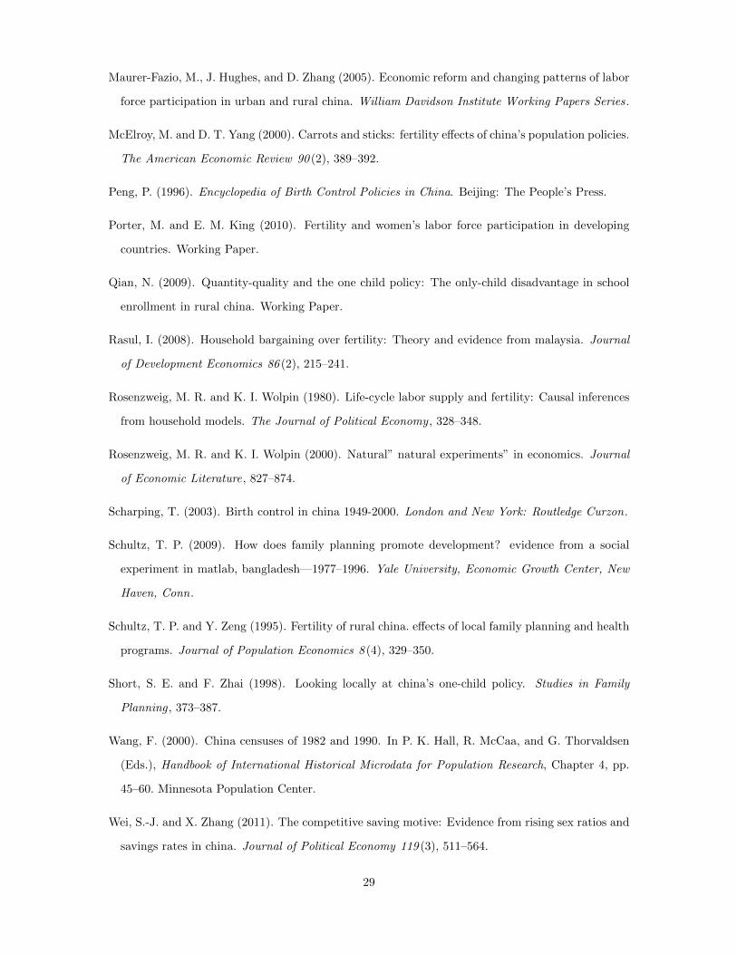
Maurer-Fazio, M., J. Hughes, and D. Zhang (2005). Economic reform and changing patterns of labor

force participation in urban and rural china. William Davidson Institute Working Papers Series.

McElroy, M. and D. T. Yang (2000). Carrots and sticks: fertility effects of china’s population policies.

The American Economic Review 90 (2), 389–392.

Peng, P. (1996). Encyclopedia of Birth Control Policies in China. Beijing: The People’s Press.

Porter, M. and E. M. King (2010). Fertility and women’s labor force participation in developing

countries. Working Paper.

Qian, N. (2009). Quantity-quality and the one child policy: The only-child disadvantage in school

enrollment in rural china. Working Paper.

Rasul, I. (2008). Household bargaining over fertility: Theory and evidence from malaysia. Journal

of Development Economics 86 (2), 215–241.

Rosenzweig, M. R. and K. I. Wolpin (1980). Life-cycle labor supply and fertility: Causal inferences

from household models. The Journal of Political Economy , 328–348.

Rosenzweig, M. R. and K. I. Wolpin (2000). Natural” natural experiments” in economics. Journal

of Economic Literature, 827–874.

Scharping, T. (2003). Birth control in china 1949-2000. London and New York: Routledge Curzon.

Schultz, T. P. (2009). How does family planning promote development? evidence from a social

experiment in matlab, bangladesh—1977–1996. Yale University, Economic Growth Center, New

Haven, Conn.

Schultz, T. P. and Y. Zeng (1995). Fertility of rural china. effects of local family planning and health

programs. Journal of Population Economics 8 (4), 329–350.

Short, S. E. and F. Zhai (1998). Looking locally at china’s one-child policy. Studies in Family

Planning , 373–387.

Wang, F. (2000). China censuses of 1982 and 1990. In P. K. Hall, R. McCaa, and G. Thorvaldsen

(Eds.), Handbook of International Historical Microdata for Population Research, Chapter 4, pp.

45–60. Minnesota Population Center.

Wei, S.-J. and X. Zhang (2011). The competitive saving motive: Evidence from rising sex ratios and

savings rates in china. Journal of Political Economy 119 (3), 511–564.

29

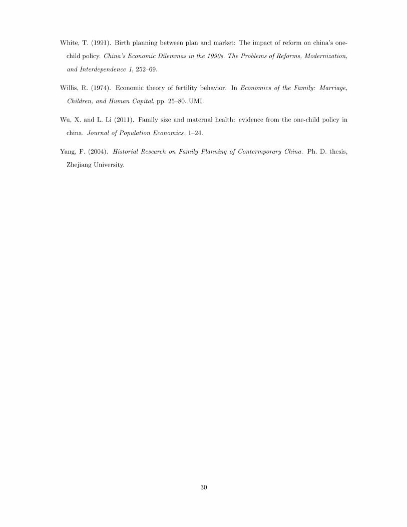
White, T. (1991). Birth planning between plan and market: The impact of reform on china’s one-

child policy. China’s Economic Dilemmas in the 1990s. The Problems of Reforms, Modernization,

and Interdependence 1, 252–69.

Willis, R. (1974). Economic theory of fertility behavior. In Economics of the Family: Marriage,

Children, and Human Capital, pp. 25–80. UMI.

Wu, X. and L. Li (2011). Family size and maternal health: evidence from the one-child policy in

china. Journal of Population Economics, 1–24.

Yang, F. (2004). Historial Research on Family Planning of Contermporary China. Ph. D. thesis,

Zhejiang University.

30

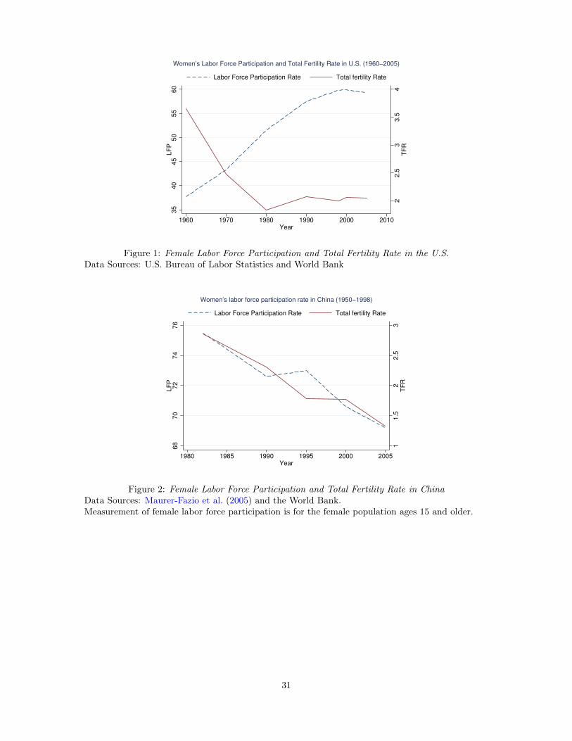
22

.53

3.5

4T

FR

35

40

45

50

55

60

LF

P

1960 1970 1980 1990 2000 2010Year

Labor Force Participation Rate Total fertility Rate

Women’s Labor Force Participation and Total Fertility Rate in U.S. (1960−2005)

Figure 1: Female Labor Force Participation and Total Fertility Rate in the U.S.Data Sources: U.S. Bureau of Labor Statistics and World Bank

11

.52

2.5

3T

FR

68

70

72

74

76

LF

P

1980 1985 1990 1995 2000 2005Year

Labor Force Participation Rate Total fertility Rate

Women’s labor force participation rate in China (1950−1998)

Figure 2: Female Labor Force Participation and Total Fertility Rate in ChinaData Sources: Maurer-Fazio et al. (2005) and the World Bank.Measurement of female labor force participation is for the female population ages 15 and older.

31

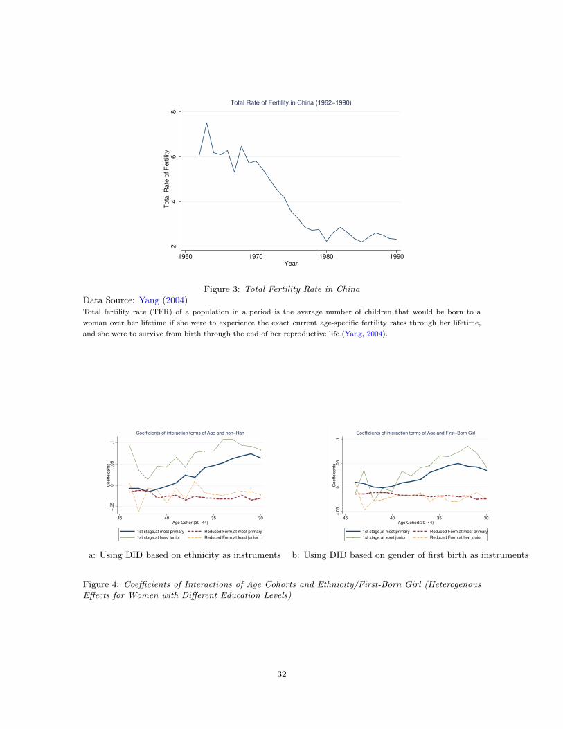
24

68

To

tal R

ate

of

Fe

rtili

ty

1960 1970 1980 1990Year

Total Rate of Fertility in China (1962−1990)

Figure 3: Total Fertility Rate in ChinaData Source: Yang (2004)Total fertility rate (TFR) of a population in a period is the average number of children that would be born to a

woman over her lifetime if she were to experience the exact current age-specific fertility rates through her lifetime,

and she were to survive from birth through the end of her reproductive life (Yang, 2004).

−.0

50

.05

.1C

oe

ffe

ice

nts

30354045Age Cohort(30−44)

1st stage,at most primary Reduced Form,at most primary

1st stage,at least junior Reduced Form,at least junior

Coefficients of interaction terms of Age and non−Han

−.0

50

.05

.1C

oe

ffe

ice

nts

30354045Age Cohort(30−44)

1st stage,at most primary Reduced Form,at most primary

1st stage,at least junior Reduced Form,at leat junior

Coefficients of interaction terms of Age and First−Born Girl

a: Using DID based on ethnicity as instruments b: Using DID based on gender of first birth as instruments

Figure 4: Coefficients of Interactions of Age Cohorts and Ethnicity/First-Born Girl (HeterogenousEffects for Women with Different Education Levels)

32

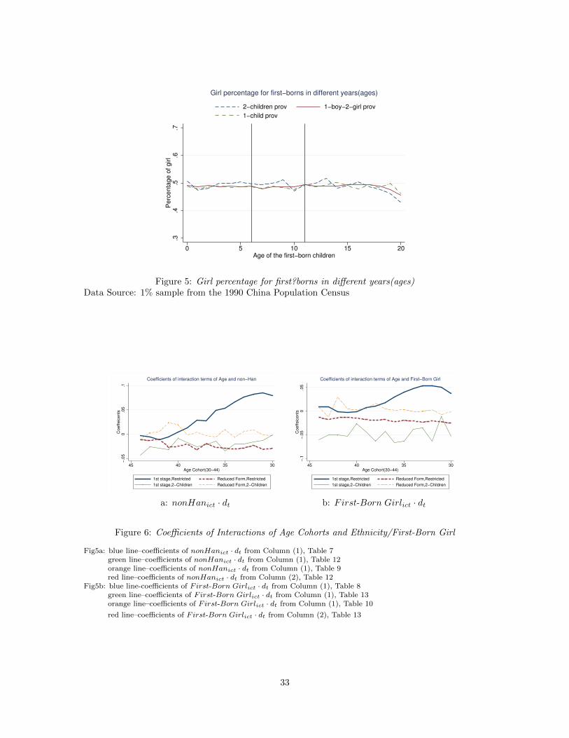
.3.4

.5.6

.7P

erc

en

tag

e o

f g

irl

0 5 10 15 20Age of the first−born children

2−children prov 1−boy−2−girl prov

1−child prov

Girl percentage for first−borns in different years(ages)

Figure 5: Girl percentage for first?borns in different years(ages)Data Source: 1% sample from the 1990 China Population Census

−.0

50

.05

.1C

oe

ffe

ice

nts

30354045Age Cohort(30−44)

1st stage,Restricted Reduced Form,Restricted

1st stage,2−Children Reduced Form,2−Children

Coefficients of interaction terms of Age and non−Han

−.1

−.0

50

.05

Co

eff

eic

en

ts

30354045Age Cohort(30−44)

1st stage,Restricted Reduced Form,Restricted

1st stage,2−Children Reduced Form,2−Children

Coefficients of interaction terms of Age and First−Born Girl

a: nonHanict · dt b: First-Born Girlict · dt

Figure 6: Coefficients of Interactions of Age Cohorts and Ethnicity/First-Born Girl

Fig5a: blue line–coefficients of nonHanict · dt from Column (1), Table 7green line–coefficients of nonHanict · dt from Column (1), Table 12orange line–coefficients of nonHanict · dt from Column (1), Table 9red line–coefficients of nonHanict · dt from Column (2), Table 12

Fig5b: blue line-coefficients of First-Born Girlict · dt from Column (1), Table 8green line–coefficients of First-Born Girlict · dt from Column (1), Table 13orange line–coefficients of First-Born Girlict · dt from Column (1), Table 10

red line–coefficients of First-Born Girlict · dt from Column (2), Table 13

33

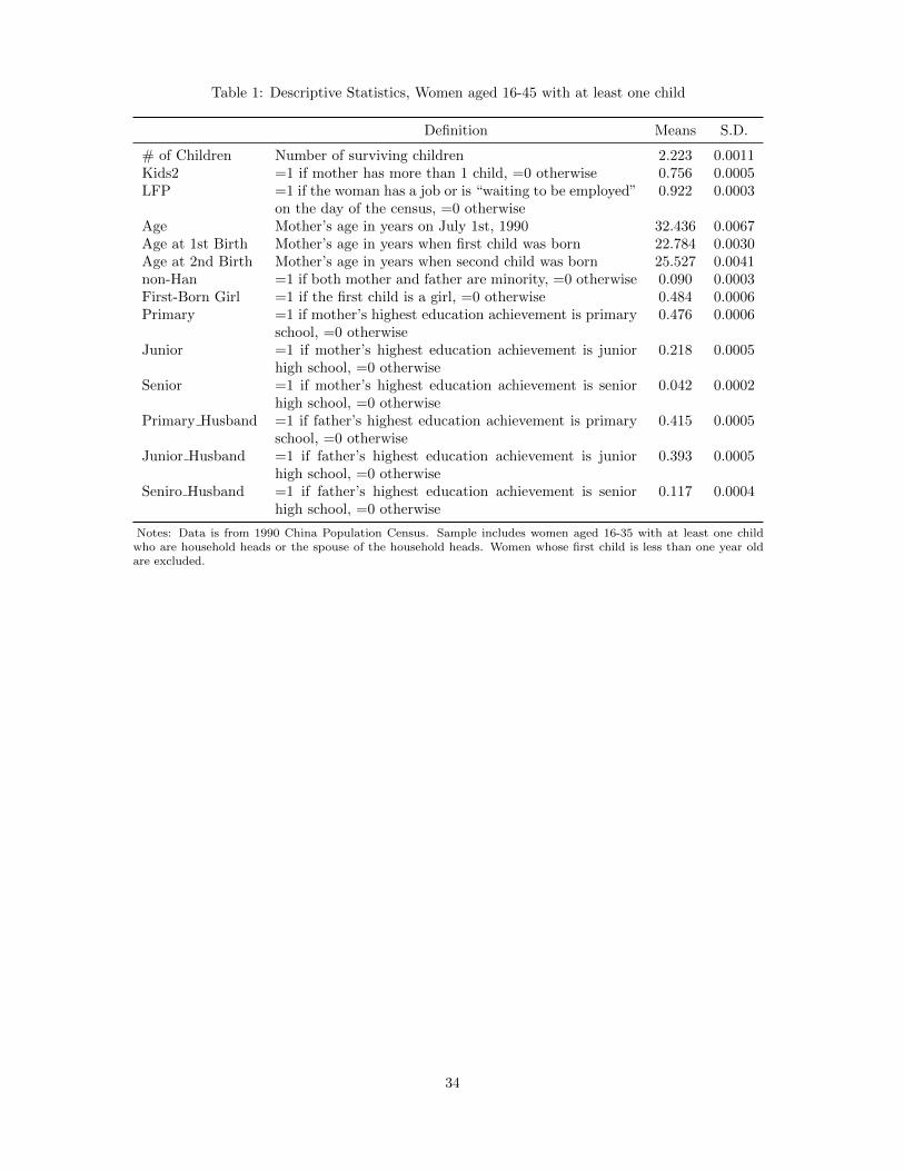
Table 1: Descriptive Statistics, Women aged 16-45 with at least one child

Definition Means S.D.

# of Children Number of surviving children 2.223 0.0011Kids2 =1 if mother has more than 1 child, =0 otherwise 0.756 0.0005LFP =1 if the woman has a job or is “waiting to be employed”

on the day of the census, =0 otherwise0.922 0.0003

Age Mother’s age in years on July 1st, 1990 32.436 0.0067Age at 1st Birth Mother’s age in years when first child was born 22.784 0.0030Age at 2nd Birth Mother’s age in years when second child was born 25.527 0.0041non-Han =1 if both mother and father are minority, =0 otherwise 0.090 0.0003First-Born Girl =1 if the first child is a girl, =0 otherwise 0.484 0.0006Primary =1 if mother’s highest education achievement is primary

school, =0 otherwise0.476 0.0006

Junior =1 if mother’s highest education achievement is juniorhigh school, =0 otherwise

0.218 0.0005

Senior =1 if mother’s highest education achievement is seniorhigh school, =0 otherwise

0.042 0.0002

Primary Husband =1 if father’s highest education achievement is primaryschool, =0 otherwise

0.415 0.0005

Junior Husband =1 if father’s highest education achievement is juniorhigh school, =0 otherwise

0.393 0.0005

Seniro Husband =1 if father’s highest education achievement is seniorhigh school, =0 otherwise

0.117 0.0004

Notes: Data is from 1990 China Population Census. Sample includes women aged 16-35 with at least one childwho are household heads or the spouse of the household heads. Women whose first child is less than one year oldare excluded.

34

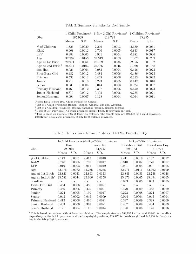
Table 2: Summary Statistics for Each Sample

1-Child Provinces1 1-Boy-2-Girl Provinces3 2-Children Provinces2

Obs. 165,969 612,785 45,855Means S.D. Means S.D. Means S.D.

# of Children 1.826 0.0020 2.296 0.0013 2.689 0.0061Kids2 0.608 0.0012 0.790 0.0005 0.843 0.0017LFP 0.984 0.0003 0.901 0.0004 0.981 0.0006Age 32.992 0.0153 32.319 0.0078 31.973 0.0289Age at 1st Birth 22.971 0.0061 22.789 0.0035 22.047 0.0132Age at 2nd Birth4 26.074 0.0103 25.486 0.0046 24.621 0.0158non-Han 0.024 0.0004 0.083 0.0004 0.416 0.0023First-Born Girl 0.482 0.0012 0.484 0.0006 0.486 0.0023Primary 0.533 0.0012 0.469 0.0006 0.353 0.0022Junior 0.218 0.0010 0.223 0.0005 0.142 0.0016Senior 0.039 0.0005 0.044 0.0003 0.024 0.0007Primary Husband 0.469 0.0012 0.397 0.0006 0.450 0.0023Junior Husband 0.379 0.0012 0.405 0.0006 0.285 0.0021Senior Husband 0.094 0.0007 0.128 0.0004 0.064 0.0011

Notes: Data is from 1990 China Population Census.1 List of 1-Child Provinces: Hainan, Yunnan, Qinghai, Ningxia, Xinjiang.2 List of 2-Children Provinces: Beijing, Shanghai, Tianjin, Jiangsu, Sichuan.3 1-Boy-2-Girl Provinces: All other provinces except Tibet, 19 provinces in total.4 This is based on mothers with at least two children. The sample sizes are 100,478 for 1-child provinces,482,842 for 1-boy-2-girl provinces, 38,597 for 2-children provinces.

Table 3: Han Vs. non-Han and First-Born Girl Vs. First-Born Boy

1-Child Provinces+1-Boy-2-Girl Provinces 1-Boy-2-Girl ProvincesHan non-Han First-born Girl First-Born Boy

Obs. 723,949 54,805 296,183 315,777Means S.D. Means S.D. Means S.D. Means S.D.

# of Children 2.179 0.0011 2.413 0.0048 2.411 0.0019 2.187 0.0017Kids2 0.748 0.0005 0.797 0.0017 0.810 0.0007 0.770 0.0007LFP 0.919 0.0003 0.911 0.0012 0.901 0.0005 0.901 0.0005Age 32.476 0.0072 32.286 0.0268 32.271 0.0111 32.362 0.0109Age at 1st Birth 22.823 0.0031 22.893 0.0123 22.841 0.0051 22.738 0.0048Age at 2nd Birth1 25.581 0.0044 25.666 0.0158 25.476 0.0065 25.494 0.0065non-Han n.a. n.a. n.a. n.a. 0.083 0.0005 0.083 0.0005First-Born Girl 0.484 0.0006 0.485 0.0021 n.a. n.a. n.a. n.a.Primary 0.486 0.0006 0.439 0.0021 0.470 0.0009 0.468 0.0009Junior 0.224 0.0005 0.199 0.0017 0.223 0.0008 0.224 0.0007Senior 0.043 0.0002 0.045 0.0009 0.044 0.0004 0.045 0.0004Primary Husband 0.412 0.0006 0.416 0.0021 0.397 0.0009 0.398 0.0009Junior Husband 0.403 0.0006 0.361 0.0021 0.407 0.0009 0.404 0.0009Senior Husband 0.121 0.0004 0.116 0.0014 0.128 0.0006 0.128 0.0006

1 This is based on mothers with at least two children. The sample sizes are 539,737 for Han and 43,583 for non-Hanrespectively in the 1-child provinces and the 1-boy-2-girl provinces, 239,597 for first-born girl and 242,830 for first-bornboy in the 1-boy-2-girl provinces.

35

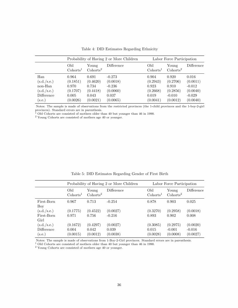
Table 4: DID Estimates Regarding Ethnicity

Probability of Having 2 or More Children Labor Force Participation

OldCohorts1

YoungCohorts2

Difference OldCohorts1

YoungCohorts2

Difference

Han 0.964 0.691 -0.273 0.904 0.920 0.016(s.d./s.e.) (0.1851) (0.4620) (0.0018) (0.2943) (0.2706) (0.0011)non-Han 0.970 0.734 -0.236 0.923 0.910 -0.012(s.d./s.e.) (0.1707) (0.4418) (0.0060) (0.2668) (0.2856) (0.0040)Difference 0.005 0.043 0.037 0.019 -0.010 -0.029(s.e.) (0.0026) (0.0021) (0.0065) (0.0041) (0.0012) (0.0040)

Notes: The sample is made of observations from the restricted provinces (the 1-child provinces and the 1-boy-2-girlprovinces). Standard errors are in parenthesis.1 Old Cohorts are consisted of mothers older than 40 but younger than 46 in 1990.2 Young Cohorts are consisted of mothers age 40 or younger.

Table 5: DID Estimates Regarding Gender of First Birth

Probability of Having 2 or More Children Labor Force Participation

OldCohorts1

YoungCohorts2

Difference OldCohorts1

YoungCohorts2

Difference

First-BornBoy

0.967 0.713 -0.254 0.878 0.903 0.025

(s.d./s.e.) (0.1775) (0.4522) (0.0027) (0.3270) (0.2958) (0.0018)First-BornGirl

0.971 0.756 -0.216 0.893 0.902 0.008

(s.d./s.e.) (0.1672) (0.4297) (0.0027) (0.3085) (0.2975) (0.0020)Difference 0.004 0.042 0.039 0.015 -0.001 -0.016(s.e.) (0.0015) (0.0012) (0.0038) (0.0028) (0.0008) (0.0027)

Notes: The sample is made of observations from 1-Boy-2-Girl provinces. Standard errors are in parenthesis.1 Old Cohorts are consisted of mothers older than 40 but younger than 46 in 1990.2 Young Cohorts are consisted of mothers age 40 or younger.

36

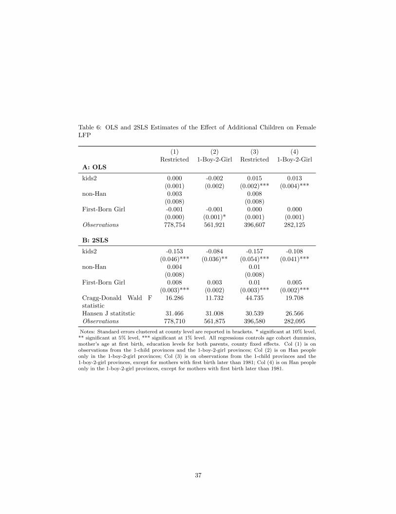
Table 6: OLS and 2SLS Estimates of the Effect of Additional Children on FemaleLFP

(1) (2) (3) (4)Restricted 1-Boy-2-Girl Restricted 1-Boy-2-Girl

A: OLS

kids2 0.000 -0.002 0.015 0.013(0.001) (0.002) (0.002)*** (0.004)***

non-Han 0.003 0.008(0.008) (0.008)

First-Born Girl -0.001 -0.001 0.000 0.000(0.000) (0.001)* (0.001) (0.001)

Observations 778,754 561,921 396,607 282,125

B: 2SLS

kids2 -0.153 -0.084 -0.157 -0.108(0.046)*** (0.036)** (0.054)*** (0.041)***

non-Han 0.004 0.01(0.008) (0.008)

First-Born Girl 0.008 0.003 0.01 0.005(0.003)*** (0.002) (0.003)*** (0.002)***

Cragg-Donald Wald Fstatistic

16.286 11.732 44.735 19.708

Hansen J statitstic 31.466 31.008 30.539 26.566Observations 778,710 561,875 396,580 282,095

Notes: Standard errors clustered at county level are reported in brackets. * significant at 10% level,** significant at 5% level, *** significant at 1% level. All regressions controls age cohort dummies,mother’s age at first birth, education levels for both parents, county fixed effects. Col (1) is onobservations from the 1-child provinces and the 1-boy-2-girl provinces; Col (2) is on Han peopleonly in the 1-boy-2-girl provinces; Col (3) is on observations from the 1-child provinces and the1-boy-2-girl provinces, except for mothers with first birth later than 1981; Col (4) is on Han peopleonly in the 1-boy-2-girl provinces, except for mothers with first birth later than 1981.

37

Table 7: Coefficients of Interaction Terms for the 1st Stage Regresssions Regarding Ethnicity

(1) (2) (1) (2)

age16*non-Han -0.028 age31*non-Han 0.085 0.082(0.070) (0.014)*** (0.012)***

age17*non-Han 0.001 age32*non-Han 0.081 0.084(0.054) (0.014)*** (0.011)***


age19*non-Han 0.072 age34*non-Han 0.066 0.079(0.039)* (0.013)*** (0.011)***


age21*non-Han 0.036 age36*non-Han 0.048 0.061(0.021)* (0.012)*** (0.009)***

age22*non-Han 0.039 age37*non-Han 0.027 0.042(0.020)** (0.012)** (0.009)***

age23*non-Han 0.068 0.712 age38*non-Han 0.028 0.035(0.019)*** (0.263)*** (0.011)** (0.009)***

age24*non-Han 0.049 0.096 age39*non-Han 0.012 0.019(0.019)*** (0.042)** (0.011) (0.009)**

age25*non-Han 0.052 0.087 age40*non-Han 0.004 0.01(0.019)*** (0.020)*** (0.011) (0.008)

age26*non-Han 0.058 0.099 age41*non-Han -0.006 0.006(0.019)*** (0.022)*** (0.011) (0.008)

age27*non-Han 0.057 0.037 age42*non-Han -0.012 -0.005(0.019)*** (0.022)* (0.011) (0.008)



age30*non-Han 0.079 0.053(0.016)*** (0.015)*** Observations 778,754 396,607

Notes: Standard errors clustered at county level are reported in brackets. * significant at 10% level, **significant at 5% level, *** significant at 1% level. All regressions controls age cohort dummies, ethnicitydummies, gender of first birth, mother’s age at first birth, education levels for both parents, county fixedeffects. Col (1) is on observations from the 1-child provinces and the 1-boy-2-girl provinces; Col (2) is onobservations from the 1-child provinces and the 1-boy-2-girl provinces, except for mothers with first birthlater than 1981.

38

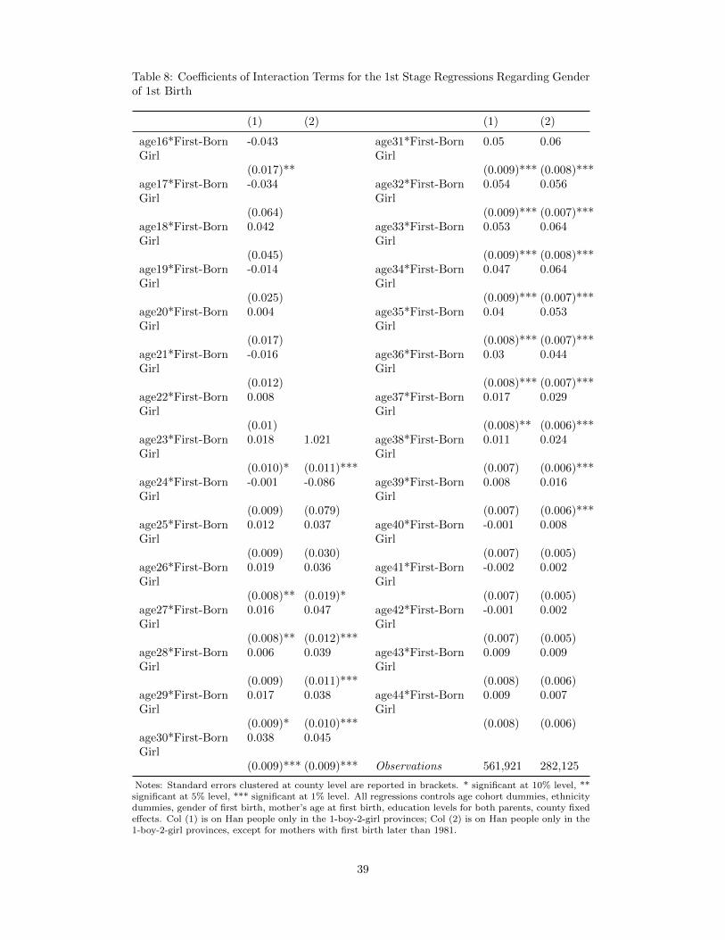
Table 8: Coefficients of Interaction Terms for the 1st Stage Regressions Regarding Genderof 1st Birth

(1) (2) (1) (2)

age16*First-BornGirl

-0.043 age31*First-BornGirl

0.05 0.06

(0.017)** (0.009)*** (0.008)***age17*First-BornGirl


0.054 0.056

(0.064) (0.009)*** (0.007)***age18*First-BornGirl

0.042 age33*First-BornGirl

0.053 0.064



0.047 0.064



0.04 0.053



0.03 0.044



0.017 0.029

(0.01) (0.008)** (0.006)***age23*First-BornGirl

0.018 1.021 age38*First-BornGirl

0.011 0.024

(0.010)* (0.011)*** (0.007) (0.006)***age24*First-BornGirl

-0.001 -0.086 age39*First-BornGirl

0.008 0.016

(0.009) (0.079) (0.007) (0.006)***age25*First-BornGirl


-0.001 0.008

(0.009) (0.030) (0.007) (0.005)age26*First-BornGirl


-0.002 0.002

(0.008)** (0.019)* (0.007) (0.005)age27*First-BornGirl


-0.001 0.002

(0.008)** (0.012)*** (0.007) (0.005)age28*First-BornGirl


0.009 0.009

(0.009) (0.011)*** (0.008) (0.006)age29*First-BornGirl


0.009 0.007

(0.009)* (0.010)*** (0.008) (0.006)age30*First-BornGirl

0.038 0.045

(0.009)*** (0.009)*** Observations 561,921 282,125

Notes: Standard errors clustered at county level are reported in brackets. * significant at 10% level, **significant at 5% level, *** significant at 1% level. All regressions controls age cohort dummies, ethnicitydummies, gender of first birth, mother’s age at first birth, education levels for both parents, county fixedeffects. Col (1) is on Han people only in the 1-boy-2-girl provinces; Col (2) is on Han people only in the1-boy-2-girl provinces, except for mothers with first birth later than 1981.

39

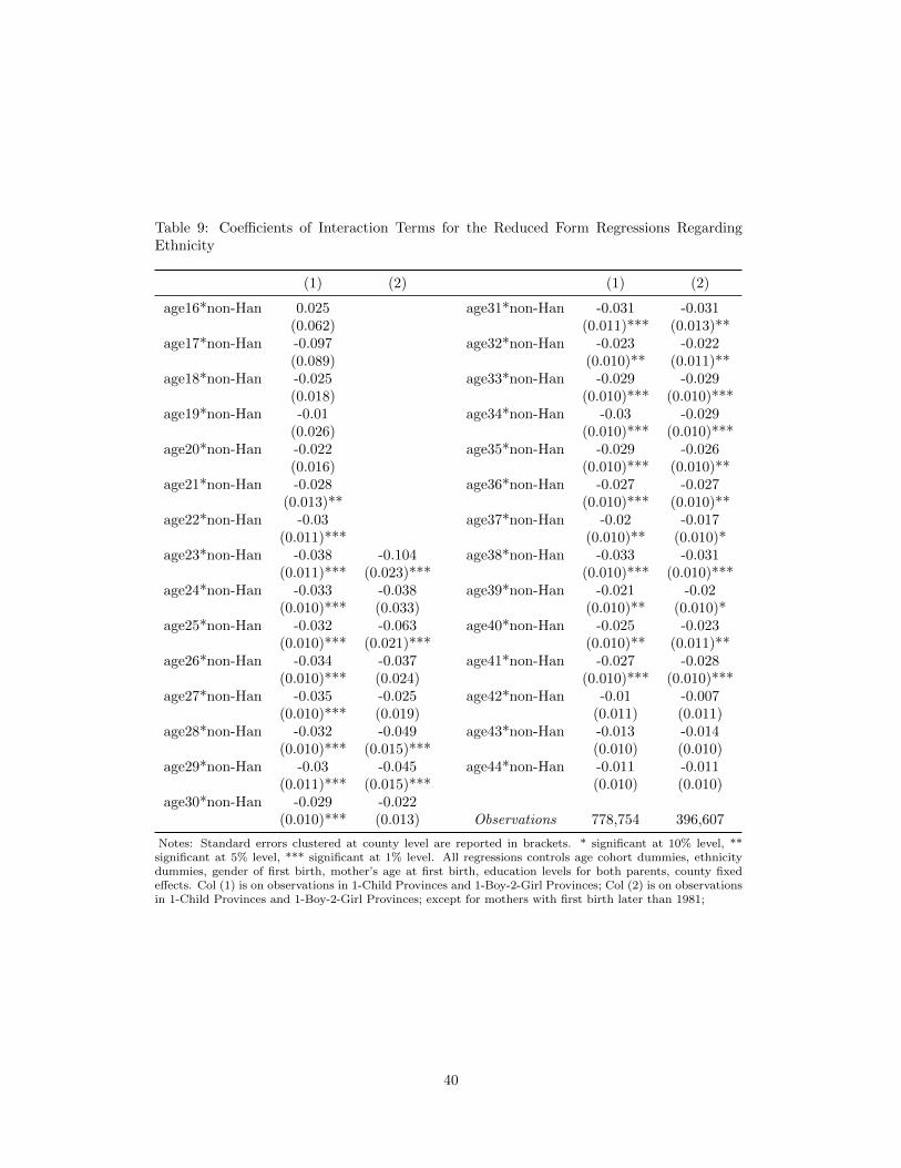
Table 9: Coefficients of Interaction Terms for the Reduced Form Regressions RegardingEthnicity

(1) (2) (1) (2)

age16*non-Han 0.025 age31*non-Han -0.031 -0.031(0.062) (0.011)*** (0.013)**

age17*non-Han -0.097 age32*non-Han -0.023 -0.022(0.089) (0.010)** (0.011)**

age18*non-Han -0.025 age33*non-Han -0.029 -0.029(0.018) (0.010)*** (0.010)***

age19*non-Han -0.01 age34*non-Han -0.03 -0.029(0.026) (0.010)*** (0.010)***

age20*non-Han -0.022 age35*non-Han -0.029 -0.026(0.016) (0.010)*** (0.010)**

age21*non-Han -0.028 age36*non-Han -0.027 -0.027(0.013)** (0.010)*** (0.010)**

age22*non-Han -0.03 age37*non-Han -0.02 -0.017(0.011)*** (0.010)** (0.010)*

age23*non-Han -0.038 -0.104 age38*non-Han -0.033 -0.031(0.011)*** (0.023)*** (0.010)*** (0.010)***

age24*non-Han -0.033 -0.038 age39*non-Han -0.021 -0.02(0.010)*** (0.033) (0.010)** (0.010)*

age25*non-Han -0.032 -0.063 age40*non-Han -0.025 -0.023(0.010)*** (0.021)*** (0.010)** (0.011)**

age26*non-Han -0.034 -0.037 age41*non-Han -0.027 -0.028(0.010)*** (0.024) (0.010)*** (0.010)***

age27*non-Han -0.035 -0.025 age42*non-Han -0.01 -0.007(0.010)*** (0.019) (0.011) (0.011)

age28*non-Han -0.032 -0.049 age43*non-Han -0.013 -0.014(0.010)*** (0.015)*** (0.010) (0.010)

age29*non-Han -0.03 -0.045 age44*non-Han -0.011 -0.011(0.011)*** (0.015)*** (0.010) (0.010)

age30*non-Han -0.029 -0.022(0.010)*** (0.013) Observations 778,754 396,607

Notes: Standard errors clustered at county level are reported in brackets. * significant at 10% level, **significant at 5% level, *** significant at 1% level. All regressions controls age cohort dummies, ethnicitydummies, gender of first birth, mother’s age at first birth, education levels for both parents, county fixedeffects. Col (1) is on observations in 1-Child Provinces and 1-Boy-2-Girl Provinces; Col (2) is on observationsin 1-Child Provinces and 1-Boy-2-Girl Provinces; except for mothers with first birth later than 1981;

40

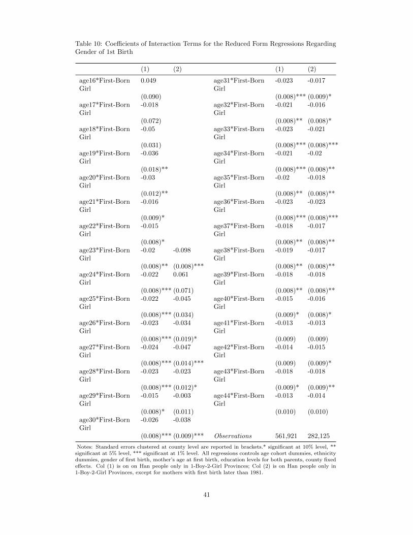
Table 10: Coefficients of Interaction Terms for the Reduced Form Regressions RegardingGender of 1st Birth

(1) (2) (1) (2)

age16*First-BornGirl


-0.023 -0.017

(0.090) (0.008)*** (0.009)*age17*First-BornGirl


-0.021 -0.016

(0.072) (0.008)** (0.008)*age18*First-BornGirl


-0.023 -0.021



-0.021 -0.02

(0.018)** (0.008)*** (0.008)**age20*First-BornGirl


-0.02 -0.018

(0.012)** (0.008)** (0.008)**age21*First-BornGirl


-0.023 -0.023

(0.009)* (0.008)*** (0.008)***age22*First-BornGirl


-0.018 -0.017

(0.008)* (0.008)** (0.008)**age23*First-BornGirl


-0.019 -0.017

(0.008)** (0.008)*** (0.008)** (0.008)**age24*First-BornGirl

-0.022 0.061 age39*First-BornGirl

-0.018 -0.018

(0.008)*** (0.071) (0.008)** (0.008)**age25*First-BornGirl


-0.015 -0.016

(0.008)*** (0.034) (0.009)* (0.008)*age26*First-BornGirl


-0.013 -0.013

(0.008)*** (0.019)* (0.009) (0.009)age27*First-BornGirl


-0.014 -0.015

(0.008)*** (0.014)*** (0.009) (0.009)*age28*First-BornGirl


-0.018 -0.018

(0.008)*** (0.012)* (0.009)* (0.009)**age29*First-BornGirl


-0.013 -0.014

(0.008)* (0.011) (0.010) (0.010)age30*First-BornGirl

-0.026 -0.038

(0.008)*** (0.009)*** Observations 561,921 282,125

Notes: Standard errors clustered at county level are reported in brackets.* significant at 10% level, **significant at 5% level, *** significant at 1% level. All regressions controls age cohort dummies, ethnicitydummies, gender of first birth, mother’s age at first birth, education levels for both parents, county fixedeffects. Col (1) is on on Han people only in 1-Boy-2-Girl Provinces; Col (2) is on Han people only in1-Boy-2-Girl Provinces, except for mothers with first birth later than 1981.

41

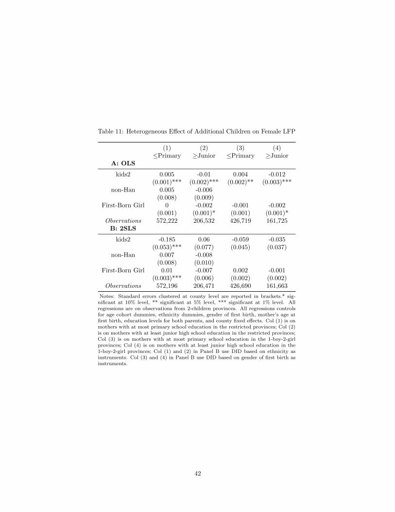
Table 11: Heterogeneous Effect of Additional Children on Female LFP

(1) (2) (3) (4)≤Primary ≥Junior ≤Primary ≥Junior

A: OLS

kids2 0.005 -0.01 0.004 -0.012(0.001)*** (0.002)*** (0.002)** (0.003)***

non-Han 0.005 -0.006(0.008) (0.009)

First-Born Girl 0 -0.002 -0.001 -0.002(0.001) (0.001)* (0.001) (0.001)*

Observations 572,222 206,532 426,719 161,725B: 2SLS

kids2 -0.185 0.06 -0.059 -0.035(0.053)*** (0.077) (0.045) (0.037)

non-Han 0.007 -0.008(0.008) (0.010)

First-Born Girl 0.01 -0.007 0.002 -0.001(0.003)*** (0.006) (0.002) (0.002)

Observations 572,196 206,471 426,690 161,663

Notes: Standard errors clustered at county level are reported in brackets.* sig-nificant at 10% level, ** significant at 5% level, *** significant at 1% level. Allregressions are on observations from 2-children provinces. All regressions controlsfor age cohort dummies, ethnicity dummies, gender of first birth, mother’s age atfirst birth, education levels for both parents, and county fixed effects. Col (1) is onmothers with at most primary school education in the restricted provinces; Col (2)is on mothers with at least junior high school education in the restricted provinces;Col (3) is on mothers with at most primary school education in the 1-boy-2-girlprovinces; Col (4) is on mothers with at least junior high school education in the1-boy-2-girl provinces; Col (1) and (2) in Panel B use DID based on ethnicity asinstruments. Col (3) and (4) in Panel B use DID based on gender of first birth asinstruments.

42

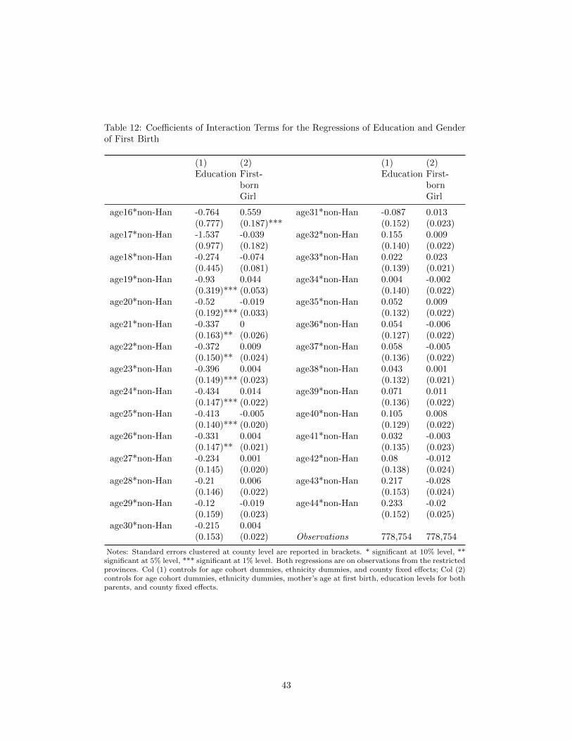
Table 12: Coefficients of Interaction Terms for the Regressions of Education and Genderof First Birth

(1) (2) (1) (2)Education First-

bornGirl

Education First-bornGirl

age16*non-Han -0.764 0.559 age31*non-Han -0.087 0.013(0.777) (0.187)*** (0.152) (0.023)

age17*non-Han -1.537 -0.039 age32*non-Han 0.155 0.009(0.977) (0.182) (0.140) (0.022)

age18*non-Han -0.274 -0.074 age33*non-Han 0.022 0.023(0.445) (0.081) (0.139) (0.021)

age19*non-Han -0.93 0.044 age34*non-Han 0.004 -0.002(0.319)*** (0.053) (0.140) (0.022)

age20*non-Han -0.52 -0.019 age35*non-Han 0.052 0.009(0.192)*** (0.033) (0.132) (0.022)

age21*non-Han -0.337 0 age36*non-Han 0.054 -0.006(0.163)** (0.026) (0.127) (0.022)

age22*non-Han -0.372 0.009 age37*non-Han 0.058 -0.005(0.150)** (0.024) (0.136) (0.022)

age23*non-Han -0.396 0.004 age38*non-Han 0.043 0.001(0.149)*** (0.023) (0.132) (0.021)

age24*non-Han -0.434 0.014 age39*non-Han 0.071 0.011(0.147)*** (0.022) (0.136) (0.022)

age25*non-Han -0.413 -0.005 age40*non-Han 0.105 0.008(0.140)*** (0.020) (0.129) (0.022)

age26*non-Han -0.331 0.004 age41*non-Han 0.032 -0.003(0.147)** (0.021) (0.135) (0.023)

age27*non-Han -0.234 0.001 age42*non-Han 0.08 -0.012(0.145) (0.020) (0.138) (0.024)

age28*non-Han -0.21 0.006 age43*non-Han 0.217 -0.028(0.146) (0.022) (0.153) (0.024)

age29*non-Han -0.12 -0.019 age44*non-Han 0.233 -0.02(0.159) (0.023) (0.152) (0.025)

age30*non-Han -0.215 0.004(0.153) (0.022) Observations 778,754 778,754

Notes: Standard errors clustered at county level are reported in brackets. * significant at 10% level, **significant at 5% level, *** significant at 1% level. Both regressions are on observations from the restrictedprovinces. Col (1) controls for age cohort dummies, ethnicity dummies, and county fixed effects; Col (2)controls for age cohort dummies, ethnicity dummies, mother’s age at first birth, education levels for bothparents, and county fixed effects.

43

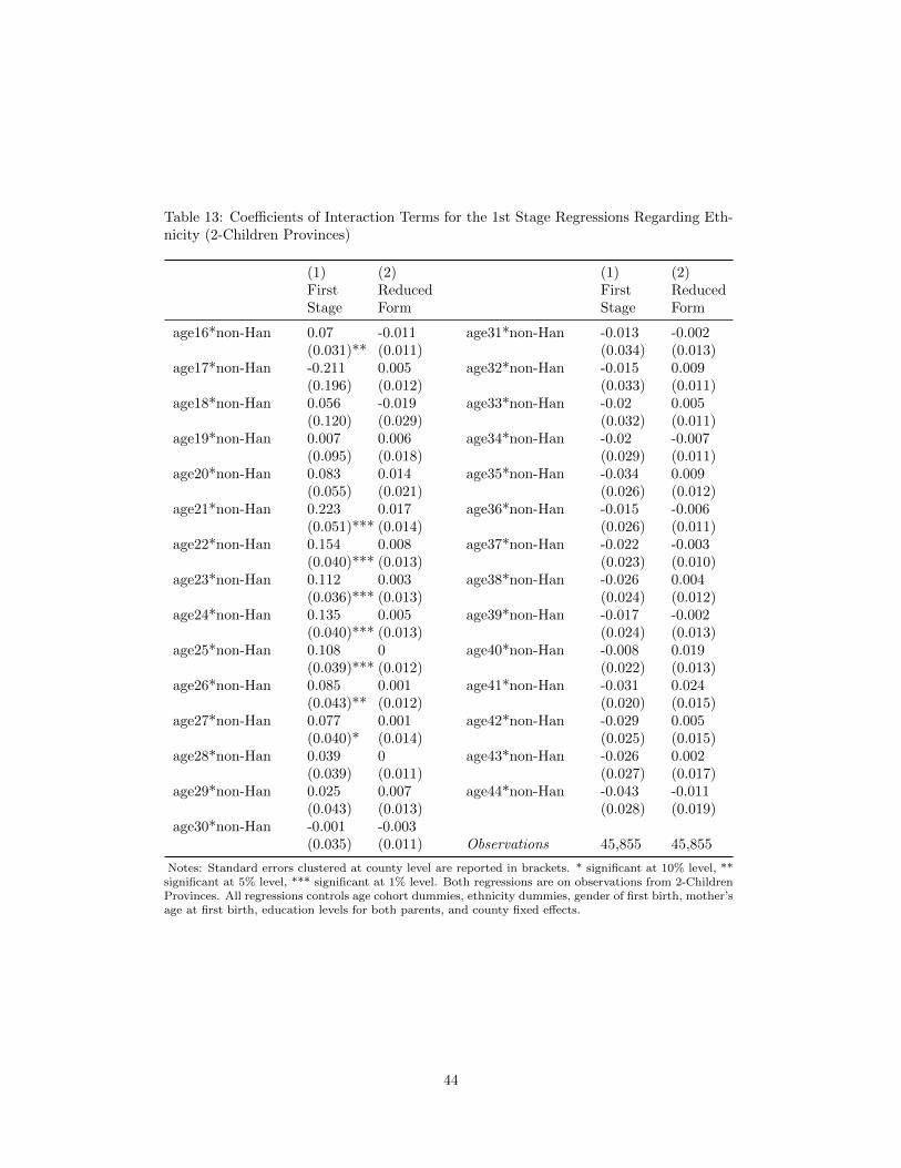
Table 13: Coefficients of Interaction Terms for the 1st Stage Regressions Regarding Eth-nicity (2-Children Provinces)

(1) (2) (1) (2)FirstStage

ReducedForm

FirstStage

ReducedForm

age16*non-Han 0.07 -0.011 age31*non-Han -0.013 -0.002(0.031)** (0.011) (0.034) (0.013)

age17*non-Han -0.211 0.005 age32*non-Han -0.015 0.009(0.196) (0.012) (0.033) (0.011)

age18*non-Han 0.056 -0.019 age33*non-Han -0.02 0.005(0.120) (0.029) (0.032) (0.011)

age19*non-Han 0.007 0.006 age34*non-Han -0.02 -0.007(0.095) (0.018) (0.029) (0.011)

age20*non-Han 0.083 0.014 age35*non-Han -0.034 0.009(0.055) (0.021) (0.026) (0.012)

age21*non-Han 0.223 0.017 age36*non-Han -0.015 -0.006(0.051)*** (0.014) (0.026) (0.011)


age23*non-Han 0.112 0.003 age38*non-Han -0.026 0.004(0.036)*** (0.013) (0.024) (0.012)


age25*non-Han 0.108 0 age40*non-Han -0.008 0.019(0.039)*** (0.012) (0.022) (0.013)

age26*non-Han 0.085 0.001 age41*non-Han -0.031 0.024(0.043)** (0.012) (0.020) (0.015)

age27*non-Han 0.077 0.001 age42*non-Han -0.029 0.005(0.040)* (0.014) (0.025) (0.015)

age28*non-Han 0.039 0 age43*non-Han -0.026 0.002(0.039) (0.011) (0.027) (0.017)

age29*non-Han 0.025 0.007 age44*non-Han -0.043 -0.011(0.043) (0.013) (0.028) (0.019)

age30*non-Han -0.001 -0.003(0.035) (0.011) Observations 45,855 45,855

Notes: Standard errors clustered at county level are reported in brackets. * significant at 10% level, **significant at 5% level, *** significant at 1% level. Both regressions are on observations from 2-ChildrenProvinces. All regressions controls age cohort dummies, ethnicity dummies, gender of first birth, mother’sage at first birth, education levels for both parents, and county fixed effects.

44

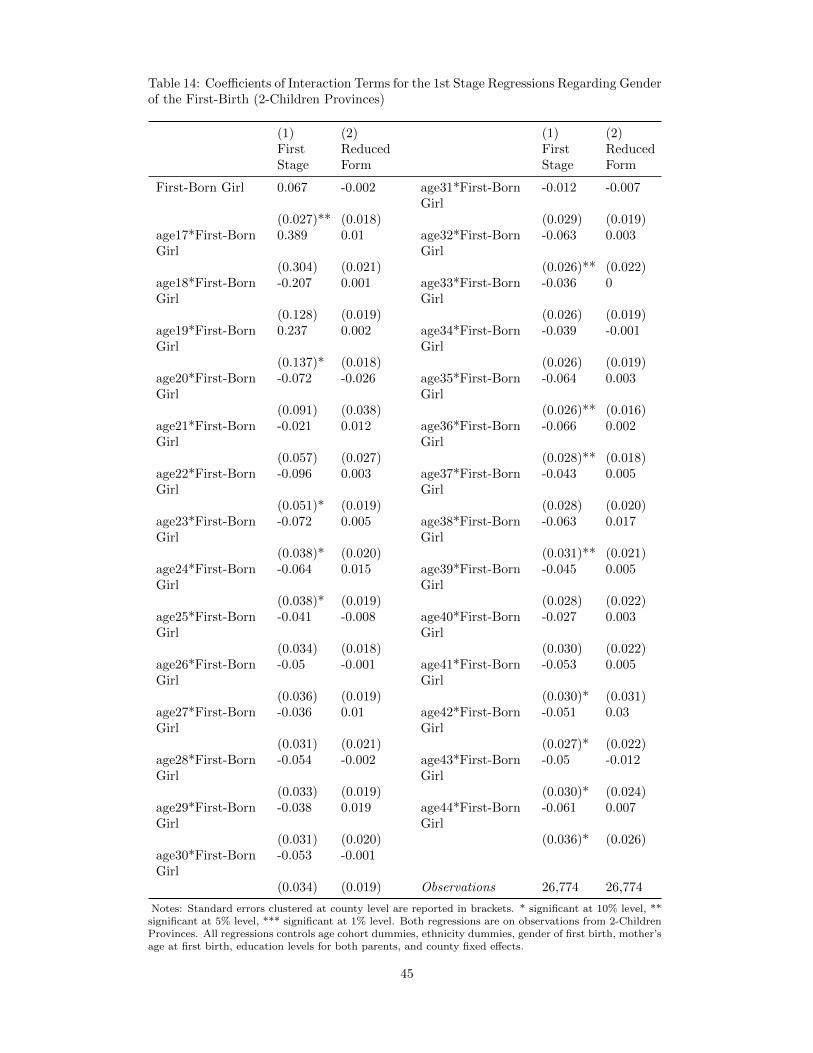
Table 14: Coefficients of Interaction Terms for the 1st Stage Regressions Regarding Genderof the First-Birth (2-Children Provinces)


ReducedForm

FirstStage

ReducedForm

First-Born Girl 0.067 -0.002 age31*First-BornGirl

-0.012 -0.007

(0.027)** (0.018) (0.029) (0.019)age17*First-BornGirl


-0.063 0.003

(0.304) (0.021) (0.026)** (0.022)age18*First-BornGirl


-0.036 0



-0.039 -0.001



-0.064 0.003



-0.066 0.002



-0.043 0.005



-0.063 0.017

(0.038)* (0.020) (0.031)** (0.021)age24*First-BornGirl


-0.045 0.005



-0.027 0.003



-0.053 0.005

(0.036) (0.019) (0.030)* (0.031)age27*First-BornGirl


-0.051 0.03



-0.05 -0.012



-0.061 0.007


-0.053 -0.001

(0.034) (0.019) Observations 26,774 26,774

Notes: Standard errors clustered at county level are reported in brackets. * significant at 10% level, **significant at 5% level, *** significant at 1% level. Both regressions are on observations from 2-ChildrenProvinces. All regressions controls age cohort dummies, ethnicity dummies, gender of first birth, mother’sage at first birth, education levels for both parents, and county fixed effects.

45

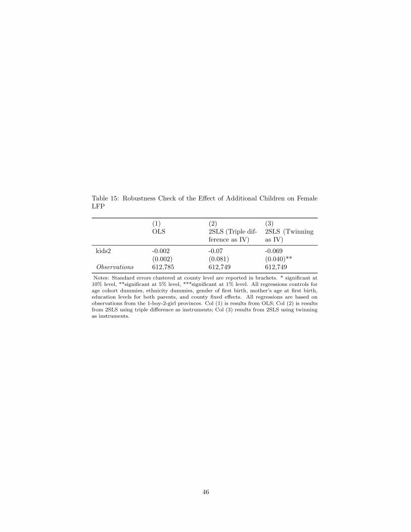
Table 15: Robustness Check of the Effect of Additional Children on FemaleLFP

(1) (2) (3)OLS 2SLS (Triple dif-

ference as IV)2SLS (Twinningas IV)

kids2 -0.002 -0.07 -0.069(0.002) (0.081) (0.040)**

Observations 612,785 612,749 612,749

Notes: Standard errors clustered at county level are reported in brackets. * significant at10% level, **significant at 5% level, ***significant at 1% level. All regressions controls forage cohort dummies, ethnicity dummies, gender of first birth, mother’s age at first birth,education levels for both parents, and county fixed effects. All regressions are based onobservations from the 1-boy-2-girl provinces. Col (1) is results from OLS; Col (2) is resultsfrom 2SLS using triple difference as instruments; Col (3) results from 2SLS using twinningas instruments.

46

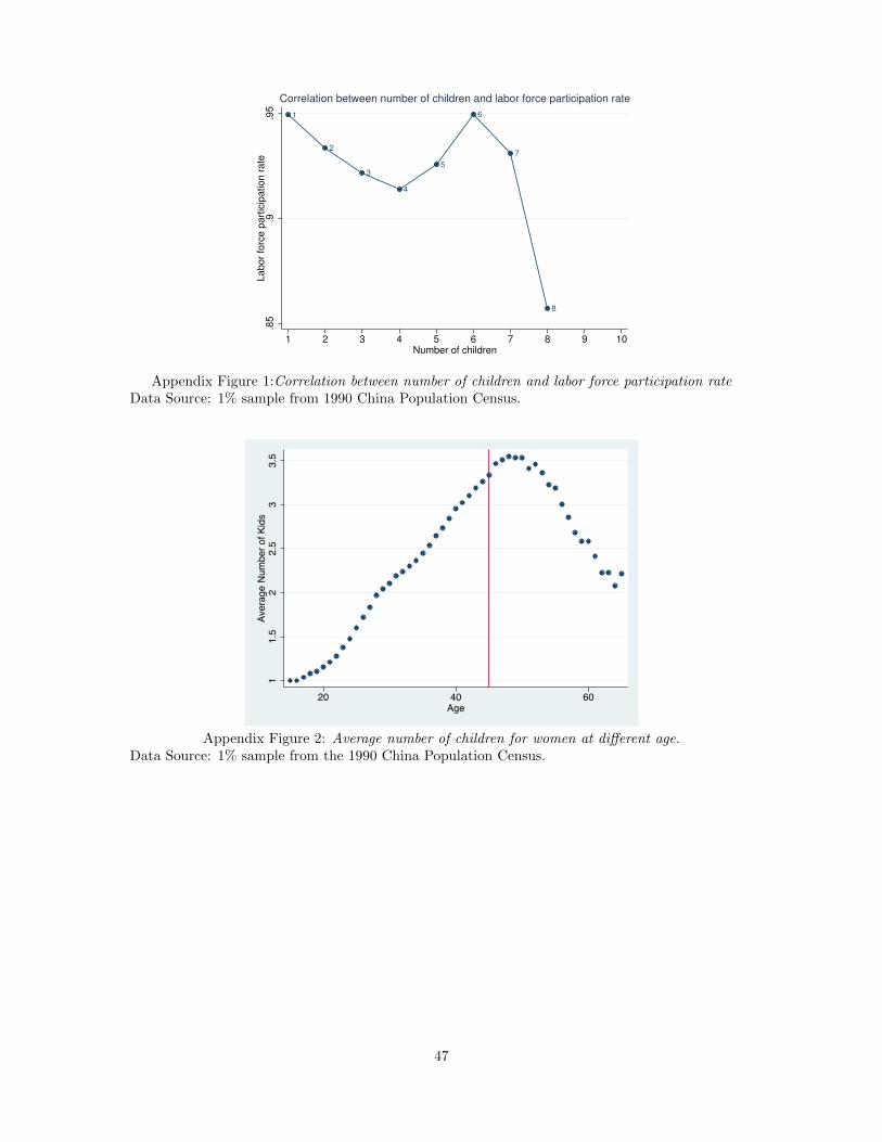
1

2

3

4

5

6

7

8

.85

.9.9

5L

ab

or

forc

e p

art

icip

atio

n r

ate

1 2 3 4 5 6 7 8 9 10Number of children

Correlation between number of children and labor force participation rate

Appendix Figure 1:Correlation between number of children and labor force participation rateData Source: 1% sample from 1990 China Population Census.

11.

52

2.5

33.

5Av

erag

e N

umbe

r of K

ids

20 40 60Age

Appendix Figure 2: Average number of children for women at different age.Data Source: 1% sample from the 1990 China Population Census.

47

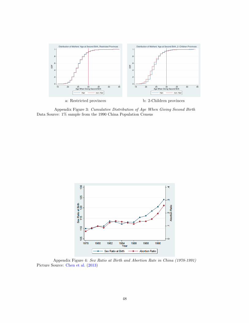
0

.2

.4

.6

.8

1

CD

F

15 20 25 30 35 40 45Age When Giving Second Birth

Han non−Han

Distribution of Mothers’ Age at Second Birth_Restricted Provinces

0

.2

.4

.6

.8

1

CD

F

15 20 25 30 35 40 45Age When Giving Second Birth

Han non−Han

Distribution of Mothers’ Age at Second Birth_2−Children Provinces

a: Restricted provinces b: 2-Children provinces

Appendix Figure 3: Cumulative Distribution of Age When Giving Second BirthData Source: 1% sample from the 1990 China Population Census

Appendix Figure 4: Sex Ratio at Birth and Abortion Rate in China (1978-1991)Picture Source: Chen et al. (2013)

48

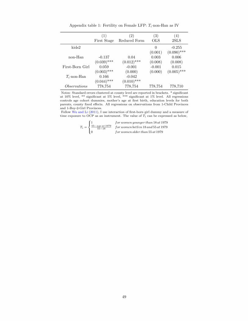
Appendix table 1: Fertility on Female LFP: Ti·non-Han as IV

(1) (2) (3) (4)First Stage Reduced Form OLS 2SLS

kids2 0 -0.255(0.001) (0.090)***

non-Han -0.137 0.04 0.003 0.006(0.039)*** (0.012)*** (0.008) (0.008)

First-Born Girl 0.059 -0.001 -0.001 0.015(0.003)*** (0.000) (0.000) (0.005)***

Ti·non-Han 0.166 -0.042(0.044)*** (0.010)***

Observations 778,754 778,754 778,754 778,710

Notes: Standard errors clustered at county level are reported in brackets. * significantat 10% level, ** significant at 5% level, *** significant at 1% level. All regressionscontrols age cohort dummies, mother’s age at first birth, education levels for bothparents, county fixed effects. All regressions on observations from 1-Child Provincesand 1-Boy-2-Girl Provinces.Follow Wu and Li (2011), I use interaction of first-born girl dummy and a measure of

time exposure to OCP as an instrument. The value of Ti can be expressed as below,

Ti =

1 for women younger than 18 at 197955−age at 1979

55−18for women betIen 18 and 55 at 1979

0 for women older than 55 at 1979

49

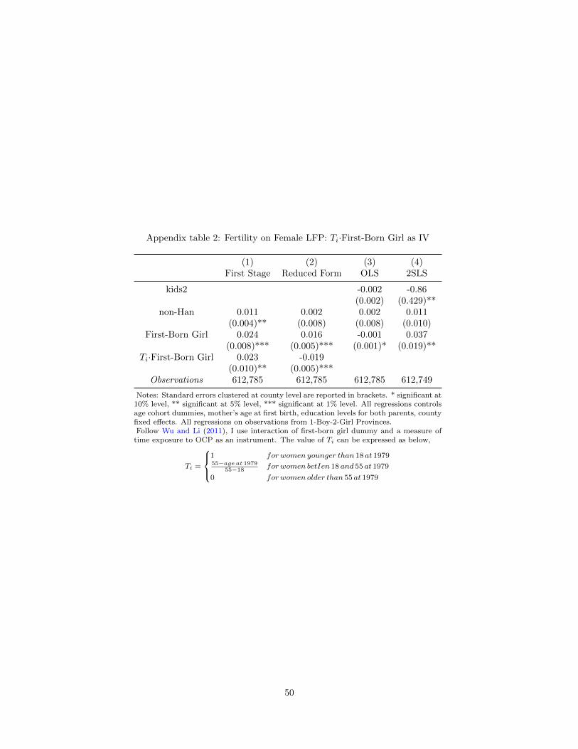
Appendix table 2: Fertility on Female LFP: Ti·First-Born Girl as IV

(1) (2) (3) (4)First Stage Reduced Form OLS 2SLS

kids2 -0.002 -0.86(0.002) (0.429)**

non-Han 0.011 0.002 0.002 0.011(0.004)** (0.008) (0.008) (0.010)

First-Born Girl 0.024 0.016 -0.001 0.037(0.008)*** (0.005)*** (0.001)* (0.019)**

Ti·First-Born Girl 0.023 -0.019(0.010)** (0.005)***

Observations 612,785 612,785 612,785 612,749

Notes: Standard errors clustered at county level are reported in brackets. * significant at10% level, ** significant at 5% level, *** significant at 1% level. All regressions controlsage cohort dummies, mother’s age at first birth, education levels for both parents, countyfixed effects. All regressions on observations from 1-Boy-2-Girl Provinces.Follow Wu and Li (2011), I use interaction of first-born girl dummy and a measure of

time exposure to OCP as an instrument. The value of Ti can be expressed as below,

Ti =

1 for women younger than 18 at 197955−age at 1979

55−18for women betIen 18 and 55 at 1979

0 for women older than 55 at 1979

50

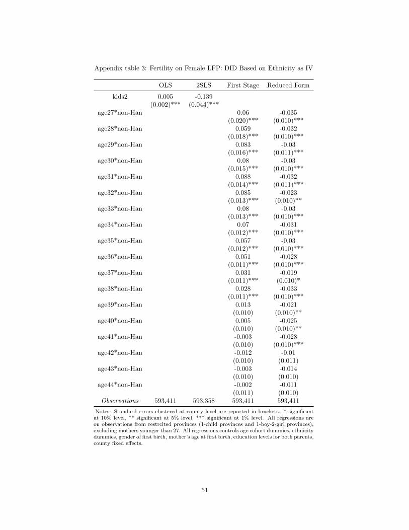
Appendix table 3: Fertility on Female LFP: DID Based on Ethnicity as IV

OLS 2SLS First Stage Reduced Form

kids2 0.005 -0.139(0.002)*** (0.044)***

age27*non-Han 0.06 -0.035(0.020)*** (0.010)***

age28*non-Han 0.059 -0.032(0.018)*** (0.010)***

age29*non-Han 0.083 -0.03(0.016)*** (0.011)***

age30*non-Han 0.08 -0.03(0.015)*** (0.010)***

age31*non-Han 0.088 -0.032(0.014)*** (0.011)***

age32*non-Han 0.085 -0.023(0.013)*** (0.010)**

age33*non-Han 0.08 -0.03(0.013)*** (0.010)***

age34*non-Han 0.07 -0.031(0.012)*** (0.010)***

age35*non-Han 0.057 -0.03(0.012)*** (0.010)***

age36*non-Han 0.051 -0.028(0.011)*** (0.010)***

age37*non-Han 0.031 -0.019(0.011)*** (0.010)*

age38*non-Han 0.028 -0.033(0.011)*** (0.010)***

age39*non-Han 0.013 -0.021(0.010) (0.010)**

age40*non-Han 0.005 -0.025(0.010) (0.010)**

age41*non-Han -0.003 -0.028(0.010) (0.010)***

age42*non-Han -0.012 -0.01(0.010) (0.011)

age43*non-Han -0.003 -0.014(0.010) (0.010)

age44*non-Han -0.002 -0.011(0.011) (0.010)

Observations 593,411 593,358 593,411 593,411

Notes: Standard errors clustered at county level are reported in brackets. * significantat 10% level, ** significant at 5% level, *** significant at 1% level. All regressions areon observations from restrcited provinces (1-child provinces and 1-boy-2-girl provinces),excluding mothers younger than 27. All regressions controls age cohort dummies, ethnicitydummies, gender of first birth, mother’s age at first birth, education levels for both parents,county fixed effects.

51

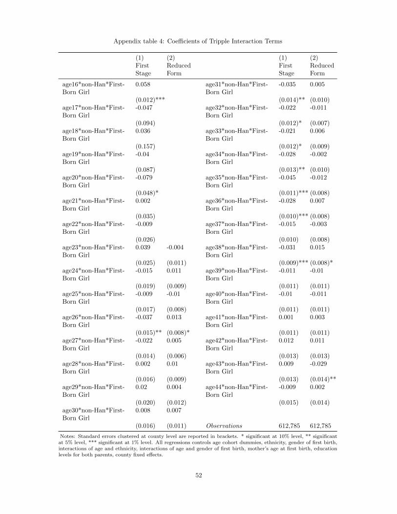
Appendix table 4: Coefficients of Tripple Interaction Terms


ReducedForm

FirstStage

ReducedForm

age16*non-Han*First-Born Girl

0.058 age31*non-Han*First-Born Girl

-0.035 0.005

(0.012)*** (0.014)** (0.010)age17*non-Han*First-Born Girl

-0.047 age32*non-Han*First-Born Girl

-0.022 -0.011

(0.094) (0.012)* (0.007)age18*non-Han*First-Born Girl


-0.021 0.006

(0.157) (0.012)* (0.009)age19*non-Han*First-Born Girl


-0.028 -0.002

(0.087) (0.013)** (0.010)age20*non-Han*First-Born Girl


-0.045 -0.012

(0.048)* (0.011)*** (0.008)age21*non-Han*First-Born Girl


-0.028 0.007

(0.035) (0.010)*** (0.008)age22*non-Han*First-Born Girl


-0.015 -0.003

(0.026) (0.010) (0.008)age23*non-Han*First-Born Girl

0.039 -0.004 age38*non-Han*First-Born Girl

-0.031 0.015

(0.025) (0.011) (0.009)*** (0.008)*age24*non-Han*First-Born Girl

-0.015 0.011 age39*non-Han*First-Born Girl

-0.011 -0.01

(0.019) (0.009) (0.011) (0.011)age25*non-Han*First-Born Girl

-0.009 -0.01 age40*non-Han*First-Born Girl

-0.01 -0.011



0.001 0.003

(0.015)** (0.008)* (0.011) (0.011)age27*non-Han*First-Born Girl


0.012 0.011


0.002 0.01 age43*non-Han*First-Born Girl

0.009 -0.029

(0.016) (0.009) (0.013) (0.014)**age29*non-Han*First-Born Girl

0.02 0.004 age44*non-Han*First-Born Girl

-0.009 0.002


0.008 0.007

(0.016) (0.011) Observations 612,785 612,785

Notes: Standard errors clustered at county level are reported in brackets. * significant at 10% level, ** significantat 5% level, *** significant at 1% level. All regressions controls age cohort dummies, ethnicity, gender of first birth,interactions of age and ethnicity, interactions of age and gender of first birth, mother’s age at first birth, educationlevels for both parents, county fixed effects.

52

fertility and female labor force participation: evidence...

Documents