ferroelectric hysteresis measurement &...
TRANSCRIPT
NPL Report CMMT(A) 152
Ferroelectric HysteresisMeasurement & Analysis
M. Stewart & M. G. CainNational Physical LaboratoryD. A. HallUniversity of Manchester
May 1999

Ferroelectric Hysteresis Measurement & Analysis
M. Stewart & M. G. CainCentre for Materials Measurement and Technology
National Physical LaboratoryTeddington, Middlesex, TW11 0LW, UK.
D. A. HallManchester Materials Science CentreUniversity of Manchester and UMIST
Manchester, M1 7HS, UK.
Summary
It has become increasingly important to characterise the performance of piezoelectric materialsunder conditions relevant to their application. Piezoelectric materials are being operated atever increasing stresses, either for high power acoustic generation or high load/stressactuation, for example. Thus, measurements of properties such as, permittivity (capacitance),dielectric loss, and piezoelectric displacement at high driving voltages are required, which canbe used either in device design or materials processing to enable the production of anenhanced, more competitive product. Techniques used to measure these properties have beendeveloped during the DTI funded CAM7 programme and this report aims to enable a user toset up one of these facilities, namely a polarisation hysteresis loop measurement system.
The report describes the technique, some example hardware implementations, and thesoftware algorithms used to perform the measurements. A version of the software is includedwhich, although does not allow control of experimental equipment, does include all theanalysis features and will allow analysis of data captured independently.

Crown copyright 1999Reproduced by permission of the Controller of HMSO
ISSN 1368-6550
May 1999
National Physical LaboratoryTeddington, Middlesex, United Kingdom, TW11 0LW
Extracts from this report may be reproduced provided the source is acknowledged.
Approved on behalf of Managing Director, NPL, by Dr C Lea, Head, Centre for MaterialsMeasurement and technology

Ferroelectric Hysteresis Measurement and Analysis
Contents1. POLARISATION-FIELD (P-E LOOPS) AND STRAIN-FIELD (S-E) MEASUREMENTS FORPIEZOELECTRIC CERAMICS................................................................................................................... 1
1.1 INTRODUCTION....................................................................................................................................... 11.2 PIEZOELECTRIC CHARACTERISATION........................................................................................................ 21.3 P-E LOOP MEASUREMENT........................................................................................................................ 4
2. HARDWARE FOR P-S-E LOOP MEASUREMENTS ............................................................................ 6
2.1 INTRODUCTION....................................................................................................................................... 62.2 HARDWARE SYSTEM................................................................................................................................ 62.3 CHOOSING HV AMPLIFIERS ..................................................................................................................... 72.4 CHOOSING DISPLACEMENT MEASUREMENT SYSTEMS FOR S-E MEASUREMENTS .......................................... 8
2.4.1 Fibre optic probe ........................................................................................................................... 82.4.2 Capacitance probe......................................................................................................................... 92.4.3 Laser interferometry ...................................................................................................................... 92.4.4 Strain gauges ............................................................................................................................... 10
2.5 CHARGE MEASUREMENT FOR P-E LOOP MEASUREMENTS......................................................................... 102.6 SUMMARY ............................................................................................................................................ 12
3. THEORETICAL BASIS FOR P-E LOOP ANALYSIS SOFTWARE................................................... 14
3.1 INTRODUCTION..................................................................................................................................... 143.2 MEASUREMENT ROUTINES..................................................................................................................... 143.3 CONSTRUCTION OF P-E AND S-E HYSTERESIS LOOPS............................................................................... 153.4 DETERMINATION OF EQUIVALENT HIGH FIELD DIELECTRIC COEFFICIENTS................................................. 173.5 RAYLEIGH LAW REPRESENTATION OF DIELECTRIC BEHAVIOUR IN PIEZOELECTRIC MATERIALS ................... 193.6 REPRESENTATION OF A LOSSY DIELECTRIC AS A PARALLEL CR NETWORK TO MODEL PE LOOPS................. 22
4. OVERVIEW OF THE SOFTWARE PACKAGE................................................................................... 23
4.1 GENERAL INFORMATION........................................................................................................................ 234.2 STARTUP AND MAIN PANEL................................................................................................................... 234.3 READ DATA FILES................................................................................................................................. 254.4 SHOW PLOTS ........................................................................................................................................ 26
4.4.1 Main Plot Window........................................................................................................................ 264.4.2 Plot Options................................................................................................................................. 27
4.5 P-E ANALYSIS...................................................................................................................................... 294.6 PROCESS DATA FILE ............................................................................................................................. 304.7 DATA ACQUISITION .............................................................................................................................. 31
4.7.1 Main Data Acquisition Window.................................................................................................... 314.7.2 Generator Setup** ........................................................................................................................ 324.7.3 Setup Inputs** ............................................................................................................................. 334.7.4 Ageing Measurements** .............................................................................................................. 35
4.8 ANALYSIS OPTIONS .............................................................................................................................. 364.9 RECALL / SAVE SETUP........................................................................................................................... 374.10 HARDWARE SUPPORT AND SETUP**..................................................................................................... 374.11 PRINTING ........................................................................................................................................... 38
5. REFERENCES......................................................................................................................................... 39
6. APPENDIX............................................................................................................................................... 40
6.1 INSTALLING THE SOFTWARE .................................................................................................................. 406.1.1 Requirements ............................................................................................................................... 406.1.2 Installing the PEHys software ...................................................................................................... 406.1.3 Running PEHys software.............................................................................................................. 406.1.4 Uninstalling the PEHys software.................................................................................................. 40

6.2 SOME EXAMPLE FILES ........................................................................................................................... 416.2.1 File: Capb.txt............................................................................................................................... 416.2.2 File: PC5H_13.hyz....................................................................................................................... 426.2.3 File: Rayleigh.txt ......................................................................................................................... 43
6.3 FILE FORMATS...................................................................................................................................... 436.3.1 Configuration File : Peconfig.txt.................................................................................................. 436.3.2 P-E and P-S-E Data Files ............................................................................................................ 47
6.4 TROUBLESHOOTING .............................................................................................................................. 496.5 RESTRICTIONS AND COPYRIGHT ............................................................................................................ 51
6.5.1 Version 1.9 CD release ................................................................................................................ 516.5.2 Licence Agreement....................................................................................................................... 51

NPL Report CMMT(A)152
1
1. Polarisation-Field (P-E loops) and Strain-Field (S-E)measurements for Piezoelectric Ceramics
1.1 Introduction
Since there is little explicit information on how to perform and interpret P-E loopmeasurements there has been a tendency to regard the measurement as somewhat academicand difficult. In fact the method is remarkably simple, and there is a lot of valuable informationthat can be gained from the measurements that can be applied by all users of piezoelectricceramics.
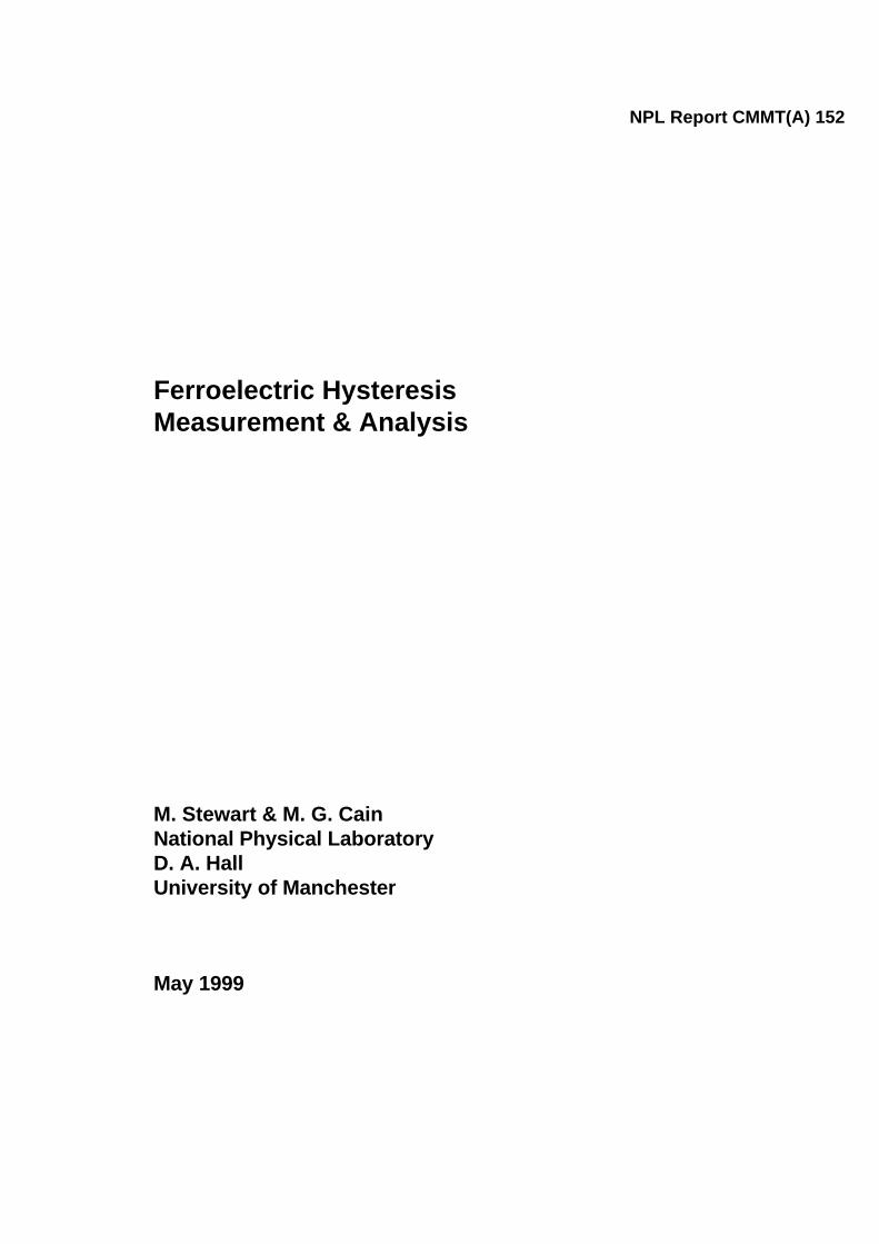
A P-E loop for a device is a plot of the charge or polarisation* (P) developed, against the fieldapplied to that device (E) at a given frequency. The significance of this measurement can bemore easily understood by examining the P-E loops for some simple linear devices. The P-Eloop for an ideal linear capacitor is a straight line whose gradient is proportional to the
* Charge and Polarisation are strictly speaking different but for materials with a high relativepermittivity we can assume they are equal.
-25
0
25
-4 0 4
Field kV/mm
Pola
risa
tion
µC
/cm
2
-25
0
25
-4 0 4
Field kV/mm
Pola
risa
tion
µC
/cm
2
Figure 1c): Lossy capacitor response Figure 1d): Non-linear ferroelectric response
-25
0
25
-4 0 4
Field kV/mm
Pola
risa
tion
µC
/cm
2
-25
0
25
-4 0 4
Field kV/mm
Pola
risa
tion
µC
/cm
2
Figure 1a): Ideal linear capacitor response Figure 1b) Ideal resistor response
NPL Report CMMT(A)152
2
capacitance (figure 1a). This is because for an ideal capacitor the current leads the voltage by90 degrees, and therefore the charge (the integral of the current with time) is in phase with thevoltage. For an ideal resistor the current and voltage are in phase and so the P-E loop is acircle with the centre at the origin (figure 1b). If these two components are combined inparallel we get the P-E loop in figure 1c which is in effect a lossy capacitor, where the areawithin the loop is proportional to the loss tangent of the device, and the slope proportional tothe capacitance. If we now consider less ideal devices such as non linear ferroelectric materialswe would get a P-E loop such as figure 1d.
The nature of piezoelectric materials is that a change in its polarisation state is coupled with apiezoelectric strain, which is the most used functional response of the material. At the timethat PE loop measurement systems were first developed, the simultaneous measurement ofthis strain (S) was difficult because of the limited availability of data capture and sensitivestrain measurement techniques. More recently, with modern computer based data acquisitionand a plethora of highly sensitive displacement measurement devices, the measurement ofstrain field (S-E) loops is more common, as is simultaneous polarisation-strain-field, (P-S-E).
1.2 Piezoelectric characterisation
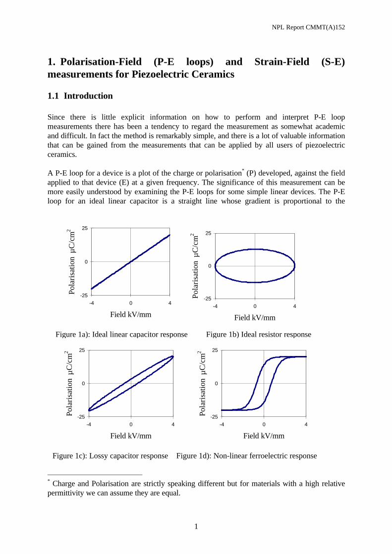
So what can the P-E loop tell us about the behaviour of a piezoelectric ceramic or device? TheIEEE standard 180 defines several reference points on the curve which enable numericcomparisons of materials. Figure 2 shows some of these; Ec, the Coercive field, Pr remanentpolarization, and Ps saturation polarisation. For a better understanding of these terms a morecomplete description of ferroelectric terminology is needed, see for example [1,2]. Theseparameters are most likely to be of interest to the material manufacturer and will give themsome indication of the poling conditions to use for the ceramic, and a better understanding ofthe material behaviour.
-25
0
25
-4 0 4
Field (Kv/mm)
Pola
risa
tion
(C
/cm
2 )
+Psat
-Psat
+Ec
-Ec
+Pr
-Pr
Figure 2. P-E hysteresis loop parameters for a ferroelectricmaterial
NPL Report CMMT(A)152
3
For the piezoelectric ceramic user there is much to be learnt from a qualitative look at the PEloop. For example the degree of non linearity of behaviour can be seen. At low fields the P-Eloop will resemble that of figure 1c for a lossy capacitor, but the loops will only begin to openout at much higher drive fields as saturation is neared (figure 1d). For achieving a controlleddisplacement with a piezoelectric actuator it may be better to confine the fields to valueswhere the behaviour is less hysteretic. The polarisation is related to the strain and since smallcurrents are somewhat simpler to measure than small displacements the P-E loop can providea means of investigating displacement behaviour. Indeed the charge can be used in a feedbackloop to drive the piezoelectric with a non linear field to give a linear displacement [3].
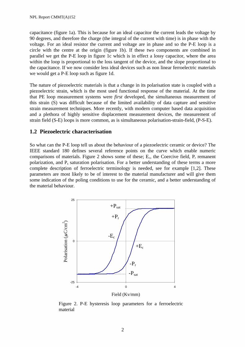
The measurement of strain field loops S-E is obviously important for actuation applications.The slope of the S-E loop is the piezoelectric coefficient, d33, one of the most important designparameters for use as actuators. The behaviour of many piezoelectric materials with respect toapplied field is highly non linear and this phenomenon can be studied with a S-E measurementsystem. The S-E loop can also show the amount of hysteresis in the strain output which isimportant when using the materials for accurate positioning applications. For high levels ofhysteresis this might mean having to use a biopolar rather than unipolar drive to return theactuator to the zero position. Measurement of S-E loops also allows investigation of theonset of massive non linearity in the strain with the appearance of the ‘butterfly loop’, figure 3.
0
50
100
150
200
250
300
350
400
450
-4 0 4
Field (Kv/mm)
Stra
in (
stra
in)
Figure 3 Schematic of a S-E loop exhibiting a butterfly loop. This schematic was simplyderived by squaring the Polarisation data from figure 2. (The strain is often, but not always,proportional to the square of the polarisation)
Using a more quantitative approach to the P-E loop it is possible to derive the capacitance andloss of the device at high fields and at different frequencies - information that is needed fortuning the drive electronics and determining the self heating effect of components.Examination of S-E loops also gives the opportunity to quantify the hysteresis in a mannersimilar to the dielectric loss, giving in effect the mechanical loss.

NPL Report CMMT(A)152
4
In some applications, such as thin film ferroelectric memories the hysteresis of the material isput to good use, and measurement of the P-E loop helps define the drive parameters and canbe used to investigate the long and short term performance.
There is an implication from definitions of parameters such as Ps, and Ec that in hysteresismeasurements the field must always be driven to saturation. However, we have seen thatvaluable information can be gained from measurements at fields well below this. Conversely,measurements need not stop at saturation, and the field can be increased until breakdownoccurs. This gives the opportunity to study breakdown behaviour, and it may even be possibleto determine a pre-breakdown characteristic.
The origin of the ‘ferro’ in ferroelectric comes from the similarity in hysteresis loop behaviourbetween ferroelectric and ferromagnetic materials, and not because they contain iron.Ferromagnetic materials can be classified as either hard or soft, dependent on their hysteresisloop behaviour. This terminology has also transferred to ferroelectric materials, where a softPZT is characterised by its low coercive field and a squareish hysteresis loop, whereas a hardPZT has a much higher coercive field and is consequently more difficult to pole and de-pole.
CSample
Cintegrating capacitorR2
R1
Oscilloscope
Figure 4 Schematic of a Sawyer Tower circuit for P-E loop measurements
1.3 P-E loop measurement
So far we have discussed the properties and significance of a hysteresis loop, but not how tomake the measurements. The measurement methods used have been developed over the yearswith advances in electronics hardware and software. The most often quoted method ofhysteresis loop measurement is based on a paper by Sawyer and Tower [4] which includedsome seminal measurements on Rochelle salt. A schematic of the experimental setup is shownin figure 4. Here the field applied across the sample is attenuated by a resistive divider, and thecurrent is integrated into charge by virtue of a large capacitor in series with the sample. Boththese voltages are then fed into the X and Y axes of an oscilloscope to generate the P-E loop.The applied voltage was usually a sinusoid at mains frequency as this was the simplest methodto generate the required voltage and current. Recording these traces using photographs of theoscilloscope screen meant that subsequent numerical analysis was difficult. As a result, severalyears later, this circuit was modified by Diamant et al [5] to include variable resistive andcapacitative components to compensate for sample conductivity and capacitance, leaving only

NPL Report CMMT(A)152
5
the non linear part. Although the use of this method proliferated the adjustment of the variablecomponents was often subjective and results unreliable.
With the advent of modern integrated circuitry the method of charge measurement haschanged from using a large capacitor, to using a virtual ground operational amplifier as acurrent to voltage converter with an integrating capacitor to convert the current to charge [6]( a more detailed examination of charge measurement methods are given later). Also, aroundthis time, the introduction of microprocessors meant that the acquisition and control was mademuch simpler, and the compensation was carried out in software rather than hardware [7].Concurrent advances in solid state high voltage electronics has meant there are commerciallyavailable high voltage amplifiers which allow frequencies other than those tied to the mainsfrequency and also enabled waveforms other than sine waves to be used. Sine waves are mostoften used since these are easily produced, however a triangle wave drive is more attractivefor frequency dependent measurements since dE/dt is constant.
The availability of cheap PC hardware, in particular digital data acquisition, has meant that themeasurement of the P-E loops has become simpler and more attention can be paid to the dataanalysis using software routines. However, there have been a few recent innovativeapproaches to the measurement of P-E loops that are worth noting. Firstly, Dickens et al [8]used a non standard drive field to isolate the non-linear components. The approach usesbipolar and unipolar fields and relies on the fact that switching only occurs in bipolar fieldswhen the field is reversed. By comparison of the various P-E loops, the resistive, capacitativeand non-linear terms can be calculated. A similar method has been used by Dias and Das-Gupta [9] but using hardware rather than software subtraction and addition of the terms. Theyuse three nominally identical samples, one sees the full bipolar field, whereas the other twosamples see respectively a positive and negative unipolar field.
The IEEE 180 standard comes the closest to defining a standard procedure for making P-Eloops but since it is only a definition of terms it is not very explicit. Most of the currentferroelectric workers describe their measurement setup for P-E loops simply as a modifiedSawyer-Tower circuit and rarely detail the compensation methods if any are used.
NPL Report CMMT(A)152
6
2. Hardware for P-S-E loop measurements
2.1 Introduction
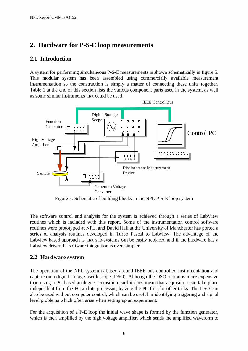
A system for performing simultaneous P-S-E measurements is shown schematically in figure 5.This modular system has been assembled using commercially available measurementinstrumentation so the construction is simply a matter of connecting these units together.Table 1 at the end of this section lists the various component parts used in the system, as wellas some similar instruments that could be used.
The software control and analysis for the system is achieved through a series of LabViewroutines which is included with this report. Some of the instrumentation control softwareroutines were prototyped at NPL, and David Hall at the University of Manchester has ported aseries of analysis routines developed in Turbo Pascal to Labview. The advantage of theLabview based approach is that sub-systems can be easily replaced and if the hardware has aLabview driver the software integration is even simpler.
2.2 Hardware system
The operation of the NPL system is based around IEEE bus controlled instrumentation andcapture on a digital storage oscilloscope (DSO). Although the DSO option is more expensivethan using a PC based analogue acquisition card it does mean that acquisition can take placeindependent from the PC and its processor, leaving the PC free for other tasks. The DSO canalso be used without computer control, which can be useful in identifying triggering and signallevel problems which often arise when setting up an experiment.
For the acquisition of a P-E loop the initial wave shape is formed by the function generator,which is then amplified by the high voltage amplifier, which sends the amplified waveform to
IEEE Control Bus
Control PC
Digital StorageScopeFunction
Generator
Displacement MeasurementDeviceSample
High VoltageAmplifier
Current to VoltageConverter
Figure 5. Schematic of building blocks in the NPL P-S-E loop system

NPL Report CMMT(A)152
7
the sample. Again the external function generator can be replaced by an internal PC digital toanalogue converter to reduce the cost. The computer control of the function generator ismainly for convenience, and for the timed ageing experiments, but it is possible to trigger thePE loops manually.
The current passing through the sample is then converted to a voltage, which is captured on adigital storage oscilloscope, along with the monitor output from the high voltage amplifier,and waveforms from any displacement measuring devices connected. The captured waveformsare then sent to the PC for subsequent analysis.
2.3 Choosing HV amplifiers
The choice of high voltage amplifier must be made based on several factors:
• high voltage specification• maximum drive frequency that can be maintained at the power amplification stated
(thus the transfer characteristics are important)• maximum current that can be delivered into a resistive and capacitative load• amplification linearity and distortion• input and output impedance• circuitry protection• cost
The typical operating fields of ceramic piezoelectric materials can extend to 500V/mm andeven 1kV/mm for some hard compositions, and so, depending on the sample thickness,voltages in excess of several kV are necessary. For strain measurements in order to generatesufficient displacement that can be measured using most of the commercially availablemeasurement devices, a voltage of the order of hundreds of volts, or even kilovolts needs tobe applied to the sample. Typical gains for amplifiers used for these types of experiments are100, and 1000 times, and are usually controlled by a function generator capable of only 10 voltoutputs. Depending on the capacitance of the device and the required frequency the maximumcurrent of the amplifier can quickly become limiting. The gain of the amplifiers are often fixed.However, when the sample begins to draw too much current the gain is reduced. Normally thisis not a problem, as the actual voltage is measured by means of a resistor divider networkincorporated in the amplifier, which is fixed at the amplifier gain setting. However the clippingof the amplifier as the device pulls to much current introduces unwanted harmonics, and issometimes difficult to spot. A divide by 10 or 100 oscilloscope probe can be used to doublecheck the voltage at the sample. This can also highlight poor connections to the sample, aswith high voltages it is possible to create a small air gap which quickly breaks down.
The operating frequency is usually much lower than the bandwidth of the amplifier, thelimiting factor is usually the current limit, consequently there is a possibility of introducinghigh frequency noise from driving the saturated amplifier. In acoustic emission experiments onpiezoelectrics this noise can be a problem as the high bandwidth detector can pass thesefrequencies on to the measurement system. This high frequency component is removed byadding a resistor in series with the sample (capacitor), with a value chosen such that the timeconstant is much longer than the driving frequency. For strain experiments the mechanical

NPL Report CMMT(A)152
8
noise generated by the amplifier is less of a problem than the much lower frequencyenvironmental mechanical vibration. Care must be taken to exclude the effect of this additionalcomponent in the measurements, i.e. the voltage drop is measured across the sample only.
2.4 Choosing displacement measurement systems for S-E measurements
The displacement generated by the piezoelectric effect on typical sized piezoceramic samplesis of the order of micrometres, or perhaps tens of micrometres for large multilayer stacks.Consequently, the displacement measurement method chosen must be capable of measuringthese small displacements with the necessary resolution and accuracy. Four methods that haveroutinely been used for these types of measurements are discussed further; fibre optic probe,capacitance probe, laser interferometry and strain gauges.
2.4.1 Fibre optic probe
The fibre optic probe consists of a bundle of fibres where one end of the bundle sees andilluminates the target. The other end of the bundle is split in two such that one half goes to alight source for the illumination, and the other half goes to a photodetector to measure thereflected light intensity.
The displacement of the target from the end of the fibre optic probe is measured by monitoringthe amount of light returned. The characteristic curve shows an initial region of increasinglight intensity with displacement which peaks and then asymptotically decreases to zero as thedisplacement increases further. The lower displacement region of the characteristic curve istermed the front slope region, and the higher displacement region of the characteristic curvethe back slope region. Both regions are close to linear over restricted but useful ranges ofdisplacement, and can be used for displacement measurement. For piezoelectric materials theforward measurement region is normally used, as this has the necessary high sensitivity formeasurement.
The fibre optic probe is sensitive to the reflectivity of the target and the system needs to becalibrated for each target by moving the target to find the optical peak and adjusting theoutput to some predetermined level, usually the maximum output. For experiments onpiezoceramics the electrode can be polished to improve reflectivity of the target, although inpractice it is simpler to attach a small mirror with double sided adhesive tape. The probe isalso sensitive to tilt of the target, and it is important that the target surface does not tilt duringoperation.
The major advantages of using fibre optic probes for piezoelectric displacement measurementare its simplicity, the fact that it is non contact, and the high bandwidth. The bandwidth can gointo the 100 kHz range and speed is limited by the amplification electronics. A consequence offast data acquisition is that the signal to noise ratio decreases, and so the signal must befiltered or larger samples must be used.
2.4.2 Capacitance probe
NPL Report CMMT(A)152
9
The principle of the capacitance displacement probe is very simple. Two metal plates aremounted on either side of the gap whose separation is to be measured. The plates act as acapacitor whose capacitance is inversely proportional to the gap between the plates accordingto the normal relationship. The probe plates are normally fitted with guard rings to eliminateerrors from edge effects. If a constant alternating current is passed through the capacitanceprobe, then the amplitude of the voltage generated is proportional to the gap distance.
In commercial devices the capacitance gauge can be realised by either making two isolatedsensors, with one attached to the piezoceramic, or having one sensor with the sample beingthe ground electrode. The former is usually the more accurate as it improves the signal tonoise ratio, but it does have the disadvantage that a sensor needs to be attached to the sample.The latter method is non contact as one face of the ceramic can be used as the groundelectrode.
Capacitance probes have excellent resolution particularly for small gaps. They offer a costeffective solution to displacement measurement, but the bandwidth is limited due to theexcitation signal needed to measure the capacitance. Also, the small stand off which is used tomeasure the displacement can, in failure conditions, cause flashover damaging the sensitiveelectronics of the capacitance gauge.
2.4.3 Laser interferometry
There are many variants of laser interferometric measurement systems but most are based onthe Michelson interferometer. The displacement is measured by splitting a monochromaticlight source (usually a helium neon laser) into two beams. One beam acts as a reference beamfollowing a fixed path, and the second measuring beam goes to the sample and returns to jointhe reference beam. The interference fringes created are used to determine the displacement.Usually the output from the interferometer is in the form of two signals, a sine and cosine,which describe a circle as the sample is moved. This corresponds to some integer multiple ofthe laser wavelength. For small movements it is sufficient to use analogue to digital conversionto determine the displacement. However, for fast movements over greater distances, it isnecessary to use counting techniques to determine the number of revolutions as well as eachpart of the circle. For greater velocities still, laser doppler vibrometers can be used, but thefrequencies these are usually used for are outside the scope of this guide.
Laser interferometers probably have the highest resolution of the four measurementtechniques, and almost infinite range. However they tend to be expensive and very difficult toset up. For piezoelectric ceramics it will be necessary to attach a mirror to the sample whichcan sometimes cause problems at higher frequencies. The small lateral size and high resolutionof the measurement system will be able to detect any movement in the mirror if it is not firmlyattached to the ceramic, and if it is very firmly attached will detect the movement caused bythe d31 motion.
Most Michelson interferometers are sensitive to mechanical vibrations and air movementsbetween the measurement head and the sample. One way to overcome this is to use a commonpath setup, such as a Jamin interferometer, where the reference beam closely follows thesample beam. This means any noise or air movement is also experienced by the reference beamand the noise is cancelled out.

NPL Report CMMT(A)152
10
Rather than measure the movement of just one face of the piezoceramic, a differential setupcan be devised whereby the interferometer interrogates the sample with two beams, one oneither face, thus measuring the change in thickness. Although this is obviously preferable, inpractice these systems are even more expensive and difficult to set up.
The traceable calibration of a laser interferometer is in essence very simple, all that is neededis a traceable measurement of the laser wavelength. This calibration factor is then included inthe measurement software associated with the interferometer.
2.4.4 Strain gauges
Strain gauges use the change in resistance of fine wires as they are strained to determine thestrain in the material to which they are bonded. The change in resistance is very small, and toform a useable measurement system the change in resistance of the gauge is measured using aWheatstone bridge. As the change in resistance is also sensitive to temperature often all fourarms of the bridge are made with strain gauges, where three gauges perform the temperaturecompensation, and only one gauge sees the strain.
Strain gauges are mostly used in static applications, but with suitable amplification they can beused in more dynamic situations into the kHz region. The large size of even the smallest straingauges makes it difficult to measure strain in samples less than 5mm thick, which forpiezoceramic samples can be a problem, and tend to make them more useful for measuringstrain in the d31 mode. Sample preparation for strain gauges can also be difficult, and incorrectplacement can lead to considerable errors.
The calibration of the strain gauge can be difficult in order to perform traceable measurements.Usually calibration is provided by the manufacturer in the form of a gauge factor, which is theaverage calibration of a sample of gauges of a similar batch. There are many reasons why thecalibration can be different from the manufacturer’s quoted gauge factor, such as temperature,gauge alignment, and the stress state of the sample. Individual gauges can always be calibratedin situ by comparison with a traceable method, however if this can be done it makes using thestrain gauge redundant.
2.5 Charge measurement for P-E loop measurements
For a P-E hysteresis loop system the measurement of field is very simple, usually needing nomore than a resistive potential divider. The measurement of charge is not very difficult butthere are several options that present themselves.
The simplest method is to use a large capacitor in series with the sample as in the conventionalSawyer-Tower circuit. This integrates the current and so the voltage measured across thiscapacitor is proportional to the charge. The only problem with this method is in choosing thecorrect value low loss capacitor for the particular conditions of voltage, current andfrequency.
Another approach is to use operational amplifiers used as current to voltage converters whichhave a capacitor in the feedback loop to integrate the current, to get the charge. This

NPL Report CMMT(A)152
11
technique is used in many commercial charge amplification systems. The main drawback is thatthe system is liable to drift if there is a zero offset and some careful design is needed for thesesystems.Since the data collection will be carried out by computer and there is bound to be some furtherdata manipulation, a simpler method is to measure the current rather than the charge, and usethe computer to integrate the current with respect to the time. This means that in the simplestcase, the current can be determined by measuring the voltage drop across a resistor placed inseries with the sample. This is usually only practical for currents in the mA range and for lowercurrents some further amplification systems are needed.
For simple self build construction it is easier to use an operational amplifier current to voltageconverter and perform the integration to charge at a later stage, usually in software. Figure 6shows the setup for an op amp current to voltage converter, where the current input goes tothe inverting input and the gain of the converter depends on the value of the feedback resistor,such that the current at any instant I is:
IV
Rout
st
= (where Rst = reference, or ‘standard’, resistor).
In this configuration, without the integrating capacitor, the zero offset does not present such aproblem. This means that a general purpose operational amplifier such as a 741 will proveequal to some of the more expensive high quality op amps. Depending on the gain of thecircuit a great deal of noise can be introduced into the output, and although the integration tocharge removes some of this, it is often found a capacitor is needed in the feedback loop. Thiscapacitor acts as a filter to remove some of the high frequency noise that is often present, thevalue of this capacitor depends on the gain resistor. Usually the time constant of this filterCstRst must be adjusted to at least two orders of magnitude smaller than the period of the
applied voltage. Too large a value of Cst can lead to a spurious phase shift in the currentwaveform, leading to an apparently lossy P-E loop.
Although this circuit is simple to build there is only one gain setting. It is a simple matter tointroduce various gain settings by switching in various resistors. It is also necessary to addswitchable filtering capacitors when changing gain or frequency. If it is necessary to controlthese settings via a PC, in the case of PC acquisition systems, it is probably more cost effectiveto purchase a purpose built current amplifier which produce a voltage output proportional tothe current flowing through them.
Figure 6 Operational Amplifier Current-to-Voltage Converter

NPL Report CMMT(A)152
12
One minor drawback with the current to voltage converter approach is that should there be afault condition such as sample breakdown or flashover, then the converter will receive a highvoltage spike which, without protection, willdestroy the circuitry. For the case of the self built741 based amplifier this will simply cost the fewpence for the replacement IC. However, for thecommercial kit this may involve the cost of externalrepair and recalibration of the unit. In order toprevent this a protection circuit consisting of twoback to back diodes connected between the inputand ground, and an optional current limitingresistor can be incorporated (figure 7). The criticalcharacteristics of these diodes are they should be able to withstand the high voltage and thatthe reverse current leakage should be as small as possible so as not to affect the measuredcurrent. Suitable diodes, which have been used successfully are 1N4007 although it is alwaysbest to compare P-E curves with and without protection to establish the effect of theadditional components.
2.6 Summary
The modular approach, using commercial equipment and Labview software means that thesystem is versatile and can be used with a variety of different building blocks. Proving testshave shown that the system gives very similar results to those obtained using a commercialpiezoelectric test system, and with the addition of capacitance and loss measurements at highvoltage is in fact more capable. The main drawback in going for this modular approach will bein the safety and electrical noise pollution aspects. This must be investigated by the builder ofsuch a system which is already catered for in a commercial system.
Figure 7 Protection Circuitry forCurrent-to-Voltage converter
NPL Report CMMT(A)152
13
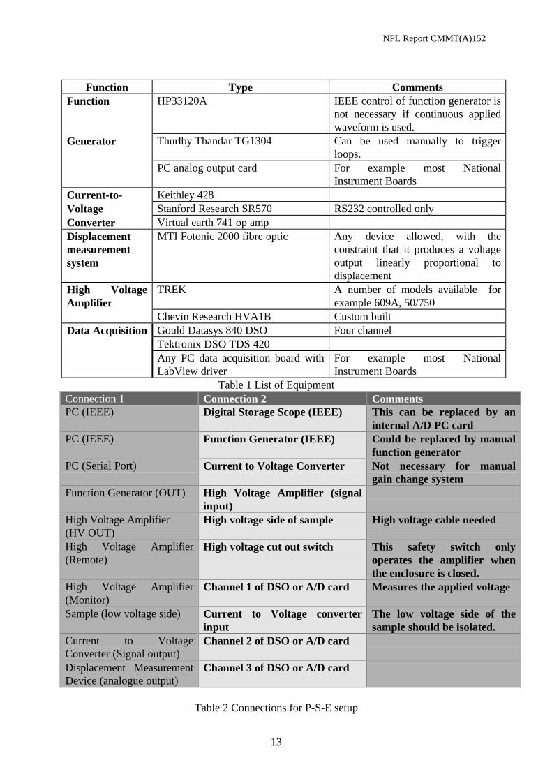
Function Type CommentsFunction HP33120A IEEE control of function generator is
not necessary if continuous appliedwaveform is used.
Generator Thurlby Thandar TG1304 Can be used manually to triggerloops.
PC analog output card For example most NationalInstrument Boards
Current-to- Keithley 428Voltage Stanford Research SR570 RS232 controlled onlyConverter Virtual earth 741 op ampDisplacementmeasurementsystem
MTI Fotonic 2000 fibre optic Any device allowed, with theconstraint that it produces a voltageoutput linearly proportional todisplacement
High VoltageAmplifier
TREK A number of models available forexample 609A, 50/750
Chevin Research HVA1B Custom builtData Acquisition Gould Datasys 840 DSO Four channel
Tektronix DSO TDS 420Any PC data acquisition board withLabView driver
For example most NationalInstrument Boards
Table 1 List of EquipmentConnection 1 Connection 2 CommentsPC (IEEE) Digital Storage Scope (IEEE) This can be replaced by an
internal A/D PC cardPC (IEEE) Function Generator (IEEE) Could be replaced by manual
function generatorPC (Serial Port) Current to Voltage Converter Not necessary for manual
gain change systemFunction Generator (OUT) High Voltage Amplifier (signal
input)High Voltage Amplifier(HV OUT)
High voltage side of sample High voltage cable needed
High Voltage Amplifier(Remote)
High voltage cut out switch This safety switch onlyoperates the amplifier whenthe enclosure is closed.
High Voltage Amplifier(Monitor)
Channel 1 of DSO or A/D card Measures the applied voltage
Sample (low voltage side) Current to Voltage converterinput
The low voltage side of thesample should be isolated.
Current to VoltageConverter (Signal output)
Channel 2 of DSO or A/D card
Displacement MeasurementDevice (analogue output)
Channel 3 of DSO or A/D card
Table 2 Connections for P-S-E setup
NPL Report CMMT(A)152
14
3. Theoretical basis for P-E loop analysis software
3.1 IntroductionThis section covers some of the theoretical basis for the software in order to help understandand use it. For further information on the development of this software and the behaviour offerroelectric ceramics under high field conditions see references [10-12].
3.2 Measurement routines
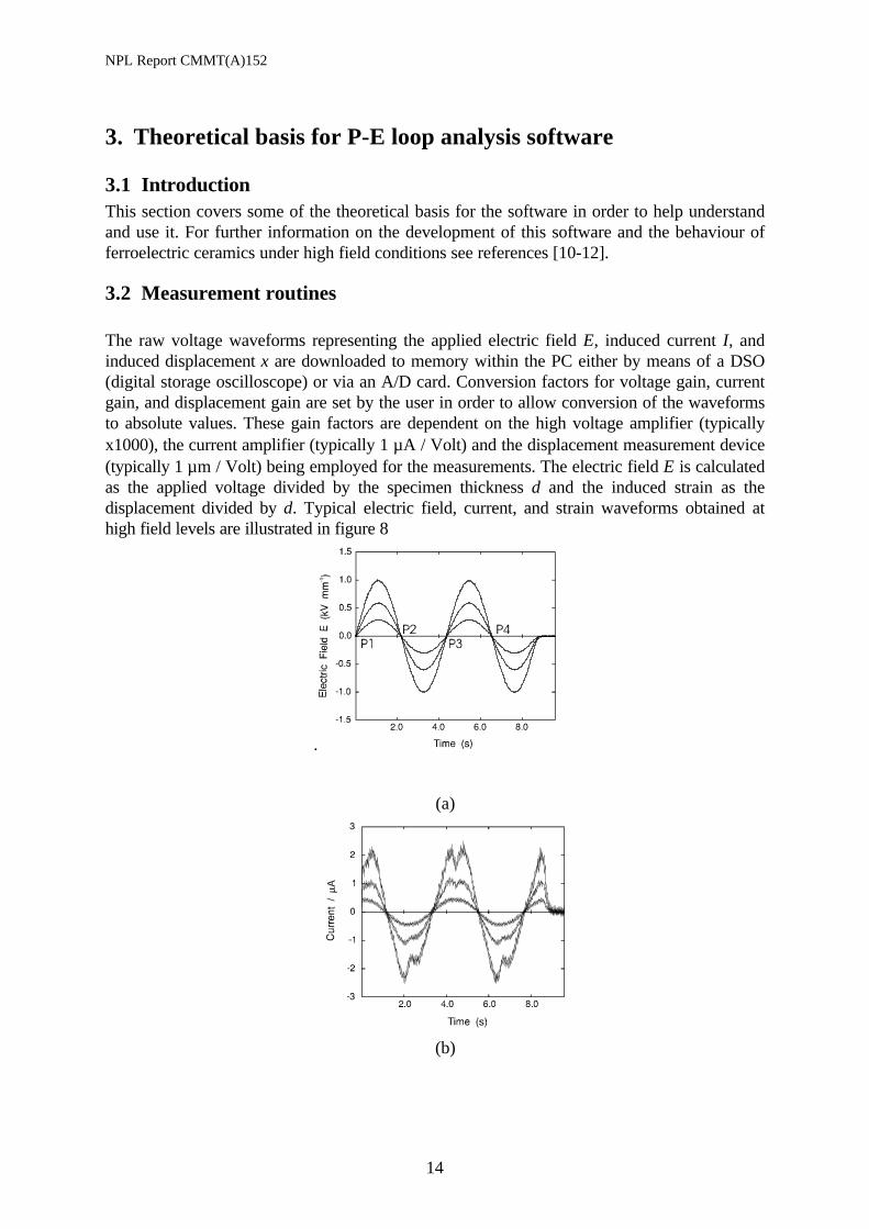
The raw voltage waveforms representing the applied electric field E, induced current I, andinduced displacement x are downloaded to memory within the PC either by means of a DSO(digital storage oscilloscope) or via an A/D card. Conversion factors for voltage gain, currentgain, and displacement gain are set by the user in order to allow conversion of the waveformsto absolute values. These gain factors are dependent on the high voltage amplifier (typicallyx1000), the current amplifier (typically 1 µA / Volt) and the displacement measurement device(typically 1 µm / Volt) being employed for the measurements. The electric field E is calculatedas the applied voltage divided by the specimen thickness d and the induced strain as thedisplacement divided by d. Typical electric field, current, and strain waveforms obtained athigh field levels are illustrated in figure 8
.
(a)
(b)

NPL Report CMMT(A)152
15
(c)
Figure 8. (a) Electric field, (b) current and (c) strain waveforms obtained for PZ26 ceramicwith an applied electric field amplitude of 3.5 kV mm-1.
3.3 Construction of P-E and S-E hysteresis loops
It is necessary to select a set of data representing a single cycle of the electric field waveform,which can then be used to construct the P-E and S-E loops. The data points corresponding tothe start and end points of the loop are identified using a ‘threshold’ routine, which detectswhen the electric field waveform crosses the horizontal time axis with either a positive ornegative slope. Thus, various zero positions can be identified, denoted as points P1, P2, P3,etc in figure 8(a). The user has the option of specifying which of these zero points will be usedto define the range of data used to construct the P-E and S-E loops. For example, for the datashown above in figure 8(a) the loops could be plotted using the data range from points P1 toP3 or points P2 to P4. For measurements made using a ‘burst’ waveform (as shown here), it isusually advisable to avoid the first half cycle of data since irreversible effects can give rise toincomplete hysteresis loops. The zero points and the threshold level can be set in the “AnalysisOptions” subroutine of the software. The threshold is initially set from the configuration filePECONFIG.TXT, usually set at 1%, although the value depends on the level of noise on thefield signal. The greater the noise the larger the value of this threshold value needs to be tocorrectly identify the crossover points.
Once the required data points have been identified, the charge Q stored by the test specimen atany given time t is calculated by numeric integration of the current data I:
Q t Idtt
t
( ) = ∫1
2
(1)
The dielectric displacement D is calculated as the surface charge density:
D tQ t
A( )
( )= (2)
where A = specimen surface area.
NPL Report CMMT(A)152
16
It is assumed that the specimen is cylindrical in shape and so:
A r= π 2(3)
where r = specimen radius.
In most cases, for high permittivity ferroelectrics, the polarisation P at a given time is verynearly equal to the dielectric displacement D. However, a small correction is needed in orderto give accurate results for low permittivity dielectrics:
D t P t E t( ) ( ) ( )= + ε0 (4)
and so:
P t D t E t( ) ( ) ( )= − ε0 (5)
The remaining problem is to define the baseline for the polarisation values. It is very difficult inpractise to determine the absolute value of polarisation, since only changes in charge (andhence polarisation) are measured. The polarisation at zero electric field strength is not alwayszero, since this can represent a positive or negative remanence Pr. As a simple solution to thisproblem, it is assumed that the maximum and minimum polarisation values, Pmax and Pmin
respectively, should be equal in magnitude
i.e. | | | |max minP P P= = 0 (6)
where P0 is the amplitude of the polarisation waveform.
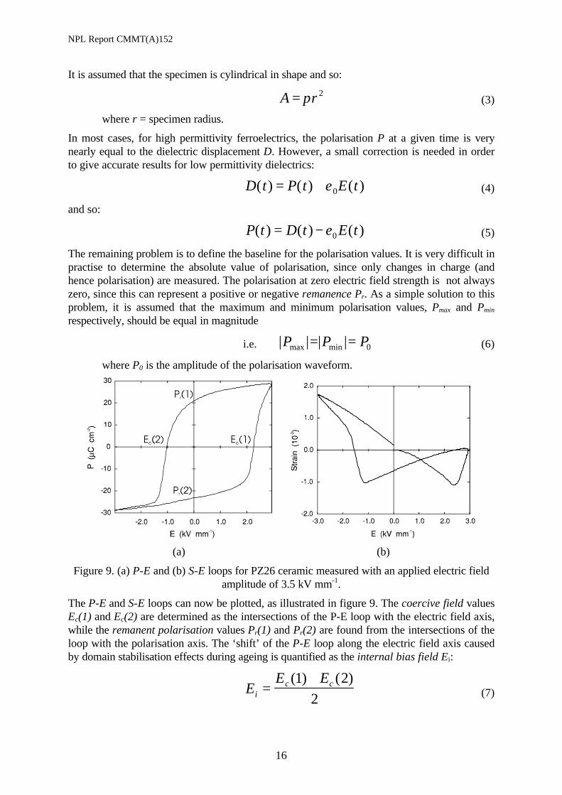
(a) (b)
Figure 9. (a) P-E and (b) S-E loops for PZ26 ceramic measured with an applied electric fieldamplitude of 3.5 kV mm-1.
The P-E and S-E loops can now be plotted, as illustrated in figure 9. The coercive field valuesEc(1) and Ec(2) are determined as the intersections of the P-E loop with the electric field axis,while the remanent polarisation values Pr(1) and Pr(2) are found from the intersections of theloop with the polarisation axis. The ‘shift’ of the P-E loop along the electric field axis causedby domain stabilisation effects during ageing is quantified as the internal bias field Ei:
EE E
ic c=
+( ) ( )1 2
2 (7)
NPL Report CMMT(A)152
17
Finally, the hysteresis loss UH is determined as the area enclosed within the P-E loop bynumerical integration:
U PdEHt
t
= ∫1
2
(8)
3.4 Determination of equivalent high field dielectric coefficients
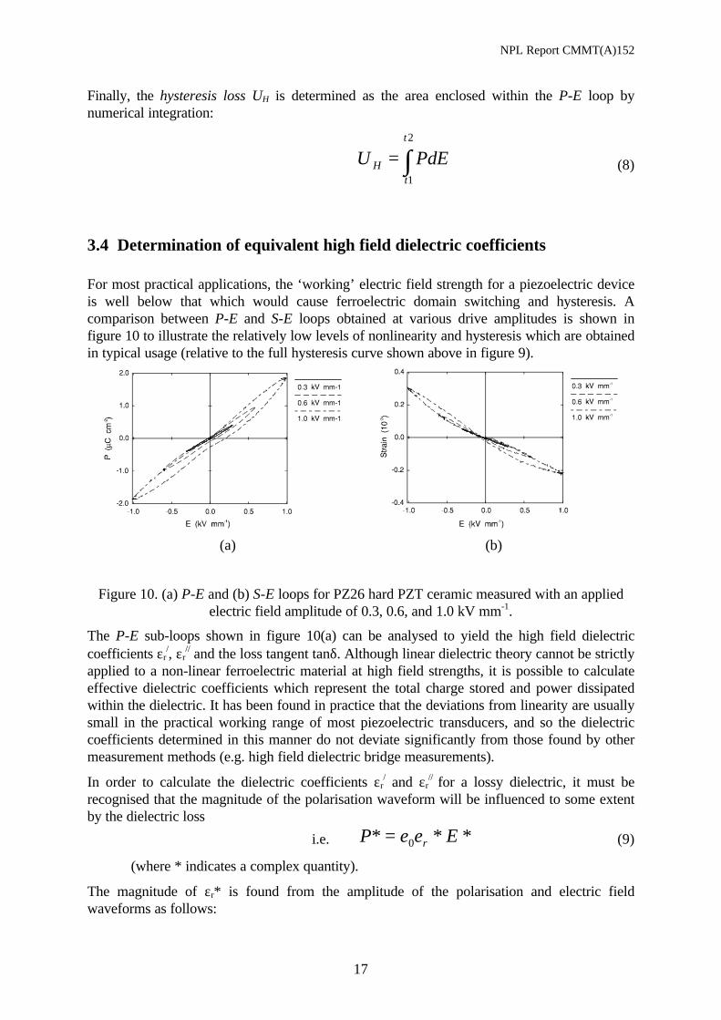
For most practical applications, the ‘working’ electric field strength for a piezoelectric deviceis well below that which would cause ferroelectric domain switching and hysteresis. Acomparison between P-E and S-E loops obtained at various drive amplitudes is shown infigure 10 to illustrate the relatively low levels of nonlinearity and hysteresis which are obtainedin typical usage (relative to the full hysteresis curve shown above in figure 9).
(a) (b)
Figure 10. (a) P-E and (b) S-E loops for PZ26 hard PZT ceramic measured with an appliedelectric field amplitude of 0.3, 0.6, and 1.0 kV mm-1.
The P-E sub-loops shown in figure 10(a) can be analysed to yield the high field dielectriccoefficients εr
/, εr// and the loss tangent tanδ. Although linear dielectric theory cannot be strictly
applied to a non-linear ferroelectric material at high field strengths, it is possible to calculateeffective dielectric coefficients which represent the total charge stored and power dissipatedwithin the dielectric. It has been found in practice that the deviations from linearity are usuallysmall in the practical working range of most piezoelectric transducers, and so the dielectriccoefficients determined in this manner do not deviate significantly from those found by othermeasurement methods (e.g. high field dielectric bridge measurements).
In order to calculate the dielectric coefficients εr/ and εr
// for a lossy dielectric, it must berecognised that the magnitude of the polarisation waveform will be influenced to some extentby the dielectric loss
i.e. P Er* * *= ε ε0 (9)
(where * indicates a complex quantity).
The magnitude of εr* is found from the amplitude of the polarisation and electric fieldwaveforms as follows:
NPL Report CMMT(A)152
18
| *|| *|
| *|ε
εr
P
E=
0(10)
The well-known expression for the power dissipated in a lossy capacitor is:
Power dissipated = 12 0
2ω δCV tan (11)
where ω = angular frequencyC = capacitance
and V0 = amplitude of applied voltage waveform.
By introducing the specimen dimensions and substituting the electric field E for the appliedvoltage V, this expression is modified to give:
Power dissipated = π ε εf Er0 02/ /
(12)
where f is the frequency of the applied AC signal.
This equation yields the energy loss per cycle, which is the hysteresis loss UH:
U EH r= πε ε0 02/ /
(13)
Subsequently, the real part of permittivity εr/ is found from these two values :
ε ε εr r r/ //(| *|) ( )= −2 2
(14)
The dielectric loss tangent tanδ is simply the ratio of εr// to εr
/ :
tan/ /
/δεε
= r
r(15)
The relationship between the applied electric field E* and the induced strain S* is analogous tothe dielectric relationship given above (equation 9), with the piezoelectric strain coefficient d*replacing the absolute dielectric permittivity ε0εr*. Therefore, the values of d/, d// and thepiezoelectric loss tangent tanδd are found as follows:
| *|| *|
| *|d
S
E= (16)
Piezoelectric ‘loss’ U SdE d Edt
t
= =∫ π / /02
1
2
(17)
d d d/ / /(| *|) ( )= −2 2(18)
and tan/ /
/δd
d
d= (19)
NPL Report CMMT(A)152
19
3.5 Rayleigh law representation of dielectric behaviour in piezoelectricmaterials
The linear nature of the εr/ vs E0 plot for PC5H is a good example of the Rayleigh law, which
is a well-known phenomenon in ferromagnetic materials [13]. The application of thisrelationship to the direct piezoelectric effect in ferroelectric PZT ceramics has been describedin some detail in a recent series of articles by Damjanovic et al. [14-16]. The form of thehysteretic relationship is thought to arise from the hindrance of domain wall motion by randomdefects (either lattice or microstructural defects). In the case of the dielectric behaviour, theRayleigh law in ferroelectrics will have the form:
ε ε αr rE E/ /( ) ( )0 00= + (20)
where εr/(0) is the value of permittivity in the low field region and α is the Rayleigh coefficient
(equal to the gradient of the εr/ vs E0 plot). In more recent work the above relationship has
been extended to include a threshold field limit below which the behaviour does not follow theRayleigh Law, however this has not been taken into account in the present implementation ofthe software. For more information on this see [12].
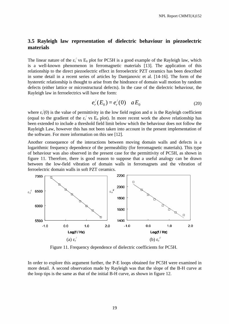
Another consequence of the interactions between moving domain walls and defects is alogarithmic frequency dependence of the permeability (for ferromagnetic materials). This typeof behaviour was also observed in the present case for the permittivity of PC5H, as shown infigure 11. Therefore, there is good reason to suppose that a useful analogy can be drawnbetween the low-field vibration of domain walls in ferromagnets and the vibration offerroelectric domain walls in soft PZT ceramics.
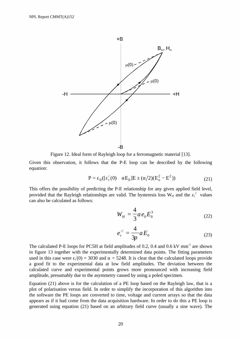
In order to explore this argument further, the P-E loops obtained for PC5H were examined inmore detail. A second observation made by Rayleigh was that the slope of the B-H curve atthe loop tips is the same as that of the initial B-H curve, as shown in figure 12.
(a) εr/ (b) εr
//
Figure 11. Frequency dependence of dielectric coefficients for PC5H.
NPL Report CMMT(A)152
20
Figure 12. Ideal form of Rayleigh loop for a ferromagnetic material [13].
Given this observation, it follows that the P-E loop can be described by the followingequation:
P E E E Er o= + ± −ε ε α α0 02 20 2([ ( ) ] ( )( ))/
(21)
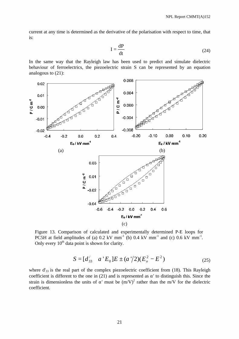
This offers the possibility of predicting the P-E relationship for any given applied field level,provided that the Rayleigh relationships are valid. The hysteresis loss WH and the εr
// valuescan also be calculated as follows:
W EH =4
3 0 03αε (22)
επ
αr E/ / =4
3 0 (23)
The calculated P-E loops for PC5H at field amplitudes of 0.2, 0.4 and 0.6 kV mm-1 are shownin figure 13 together with the experimentally determined data points. The fitting parametersused in this case were εr
/(0) = 3030 and α = 5248. It is clear that the calculated loops providea good fit to the experimental data at low field amplitudes. The deviation between thecalculated curve and experimental points grows more pronounced with increasing fieldamplitude, presumably due to the asymmetry caused by using a poled specimen.
Equation (21) above is for the calculation of a PE loop based on the Rayleigh law, that is aplot of polarisation versus field. In order to simplify the incorporation of this algorithm intothe software the PE loops are converted to time, voltage and current arrays so that the dataappears as if it had come from the data acquisition hardware. In order to do this a PE loop isgenerated using equation (21) based on an arbitrary field curve (usually a sine wave). The
NPL Report CMMT(A)152
21
current at any time is determined as the derivative of the polarisation with respect to time, thatis:
IdP
dt= (24)
In the same way that the Rayleigh law has been used to predict and simulate dielectricbehaviour of ferroelectrics, the piezoelectric strain S can be represented by an equationanalogous to (21):
S d E E E Eo= + ± −[ ' ] ( ' )( )/33 0
2 22α α (25)
where d'33 is the real part of the complex piezoelectric coefficient from (18). This Rayleighcoefficient is different to the one in (21) and is represented as α' to distinguish this. Since thestrain is dimensionless the units of α' must be (m/V)2 rather than the m/V for the dielectriccoefficient.
(a) (b)
(c)
Figure 13. Comparison of calculated and experimentally determined P-E loops forPC5H at field amplitudes of (a) 0.2 kV mm-1 (b) 0.4 kV mm-1 and (c) 0.6 kV mm-1.Only every 10th data point is shown for clarity.

NPL Report CMMT(A)152
22
3.6 Representation of a lossy dielectric as a parallel CR network to modelPE loops.
At fields below which ferroelectric switching occurs piezoelectric materials can be thought ofas a lossy linear dielectric and can simulated by a parallel resistor capacitor (RC) networkwhere the resistor R represents the dielectric loss across an ideal capacitor C. This means thecurrent across the RC model can be represented by the following:
IVR
CdVdt
= + (26)
The simulation subroutine of the software can create time, voltage current curves based on(26) given an arbitrary voltage waveform, and user input of C and R. This can be used as alearning tool for the understanding of the significance of PE loops, but can also be used tocheck the hardware system. For instance, by using a very low loss polypropylene capacitor inparallel with a high voltage resistor, measurements can be made and compared with the PEloops produced using (26). Also given that for the parallel RC circuit the dielectric loss isgiven by
tanδω
=1
RC (27)
the tan δ calculated by the software can be compared with that expected from (27).
NPL Report CMMT(A)152
23
4. Overview of the software package
4.1 General informationThe software was designed as a fully integrated set of measurement and analysis routines forthe electrical characterisation of piezoelectric ceramic materials under high field conditions. Atthe outset of the CAM7 project, it was envisaged that most emphasis would be placed ondetermination of the effective high field dielectric properties of ferroelectric ceramics atintermediate field levels (0<E0<Ec), and the saturated ferroelectric hysteresis characteristics(for E0<Ec), by the acquisition and analysis of P-E (polarisation-electric field) data. During thecourse of the software development, it became evident that it would also be important toincorporate routines for the measurement and analysis of S-E (strain-field) data, therebyenabling a calculation of the effective high field piezoelectric coefficients. Within the program,a boolean switch (P-E/P-S-E) is used as a selector to include or exclude the strain-field data.
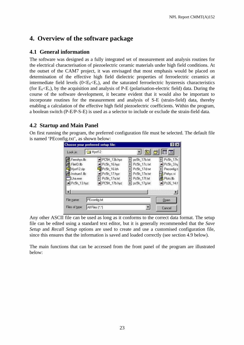
4.2 Startup and Main PanelOn first running the program, the preferred configuration file must be selected. The default fileis named ‘PEconfig.txt’, as shown below:
Any other ASCII file can be used as long as it conforms to the correct data format. The setupfile can be edited using a standard text editor, but it is generally recommended that the SaveSetup and Recall Setup options are used to create and use a customised configuration file,since this ensures that the information is saved and loaded correctly (see section 4.9 below).
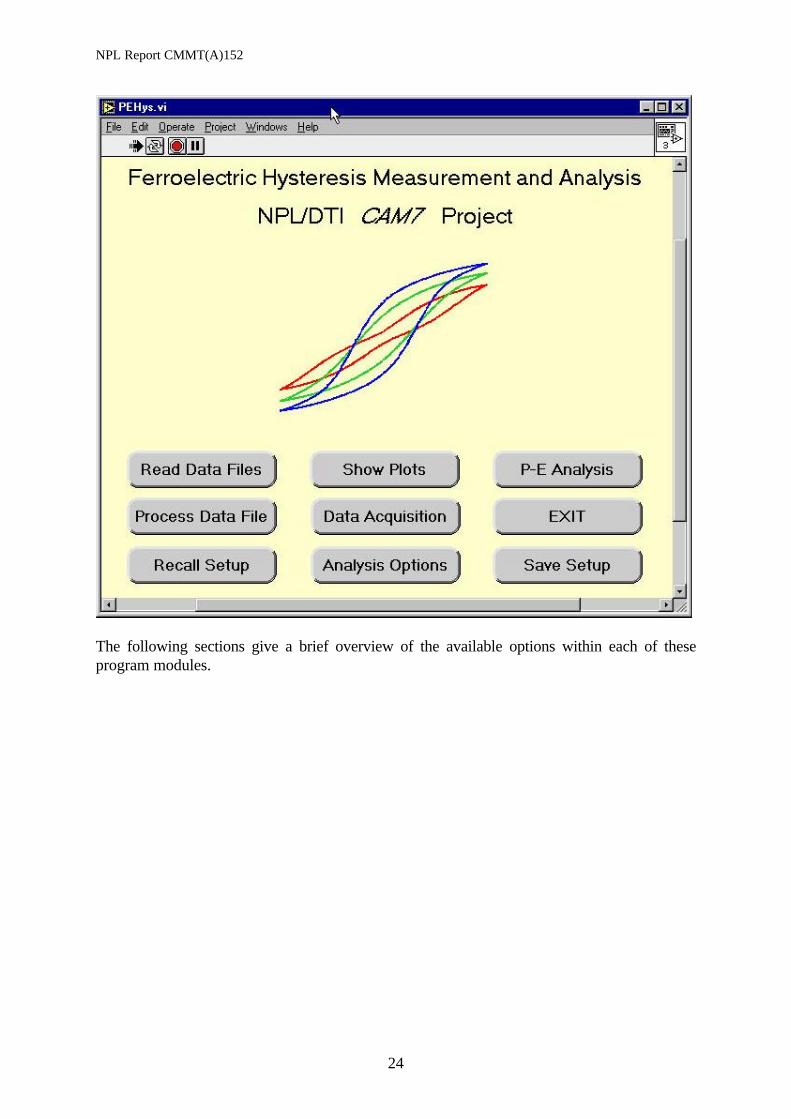
The main functions that can be accessed from the front panel of the program are illustratedbelow:
NPL Report CMMT(A)152
24
The following sections give a brief overview of the available options within each of theseprogram modules.
NPL Report CMMT(A)152
25
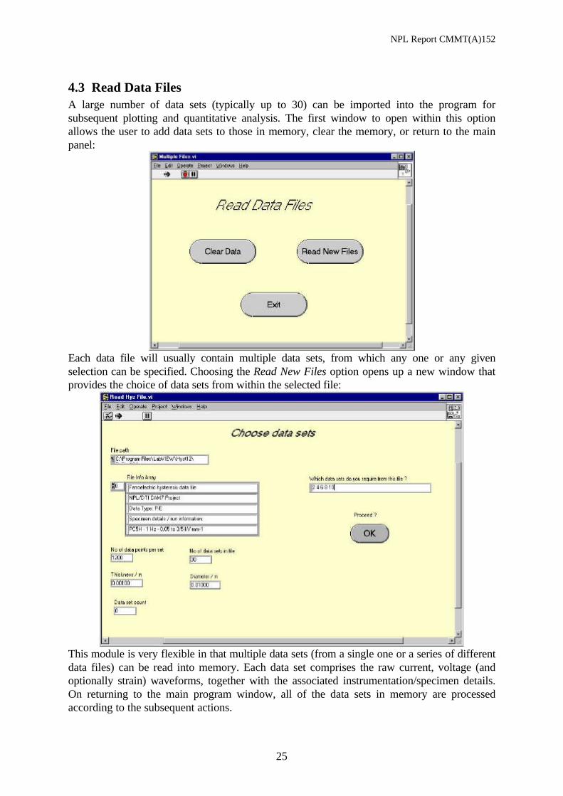
4.3 Read Data FilesA large number of data sets (typically up to 30) can be imported into the program forsubsequent plotting and quantitative analysis. The first window to open within this optionallows the user to add data sets to those in memory, clear the memory, or return to the mainpanel:
Each data file will usually contain multiple data sets, from which any one or any givenselection can be specified. Choosing the Read New Files option opens up a new window thatprovides the choice of data sets from within the selected file:
This module is very flexible in that multiple data sets (from a single one or a series of differentdata files) can be read into memory. Each data set comprises the raw current, voltage (andoptionally strain) waveforms, together with the associated instrumentation/specimen details.On returning to the main program window, all of the data sets in memory are processedaccording to the subsequent actions.
NPL Report CMMT(A)152
26
4.4 Show Plots
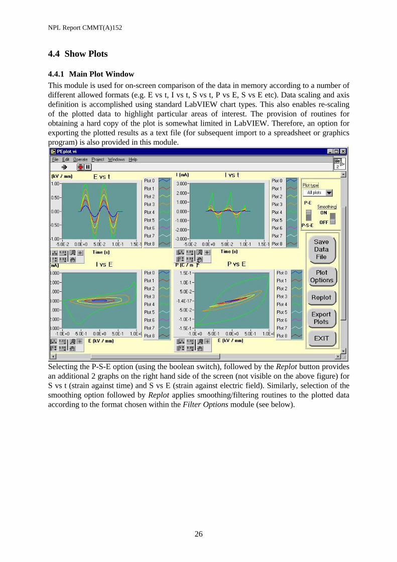
4.4.1 Main Plot WindowThis module is used for on-screen comparison of the data in memory according to a number ofdifferent allowed formats (e.g. E vs t, I vs t, S vs t, P vs E, S vs E etc). Data scaling and axisdefinition is accomplished using standard LabVIEW chart types. This also enables re-scalingof the plotted data to highlight particular areas of interest. The provision of routines forobtaining a hard copy of the plot is somewhat limited in LabVIEW. Therefore, an option forexporting the plotted results as a text file (for subsequent import to a spreadsheet or graphicsprogram) is also provided in this module.
Selecting the P-S-E option (using the boolean switch), followed by the Replot button providesan additional 2 graphs on the right hand side of the screen (not visible on the above figure) forS vs t (strain against time) and S vs E (strain against electric field). Similarly, selection of thesmoothing option followed by Replot applies smoothing/filtering routines to the plotted dataaccording to the format chosen within the Filter Options module (see below).
NPL Report CMMT(A)152
27
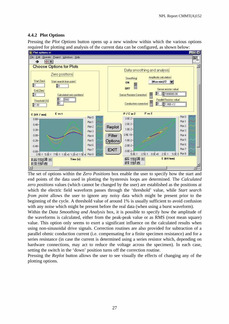
4.4.2 Plot OptionsPressing the Plot Options button opens up a new window within which the various optionsrequired for plotting and analysis of the current data can be configured, as shown below:
The set of options within the Zero Positions box enable the user to specify how the start andend points of the data used in plotting the hysteresis loops are determined. The Calculatedzero positions values (which cannot be changed by the user) are established as the positions atwhich the electric field waveform passes through the ‘threshold’ value, while Start searchfrom point allows the user to ignore any noisy data which might be present prior to thebeginning of the cycle. A threshold value of around 1% is usually sufficient to avoid confusionwith any noise which might be present before the real data (when using a burst waveform).Within the Data Smoothing and Analysis box, it is possible to specify how the amplitude ofthe waveforms is calculated, either from the peak-peak value or as RMS (root mean square)value. This option only seems to exert a significant influence on the calculated results whenusing non-sinusoidal drive signals. Correction routines are also provided for subtraction of aparallel ohmic conduction current (i.e. compensating for a finite specimen resistance) and for aseries resistance (in case the current is determined using a series resistor which, depending onhardware connections, may act to reduce the voltage across the specimen). In each case,setting the switch in the ‘down’ position turns off the correction routine.Pressing the Replot button allows the user to see visually the effects of changing any of theplotting options.
NPL Report CMMT(A)152
28
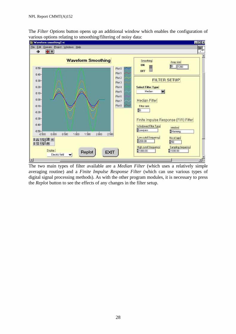
The Filter Options button opens up an additional window which enables the configuration ofvarious options relating to smoothing/filtering of noisy data:
The two main types of filter available are a Median Filter (which uses a relatively simpleaveraging routine) and a Finite Impulse Response Filter (which can use various types ofdigital signal processing methods). As with the other program modules, it is necessary to pressthe Replot button to see the effects of any changes in the filter setup.
NPL Report CMMT(A)152
29
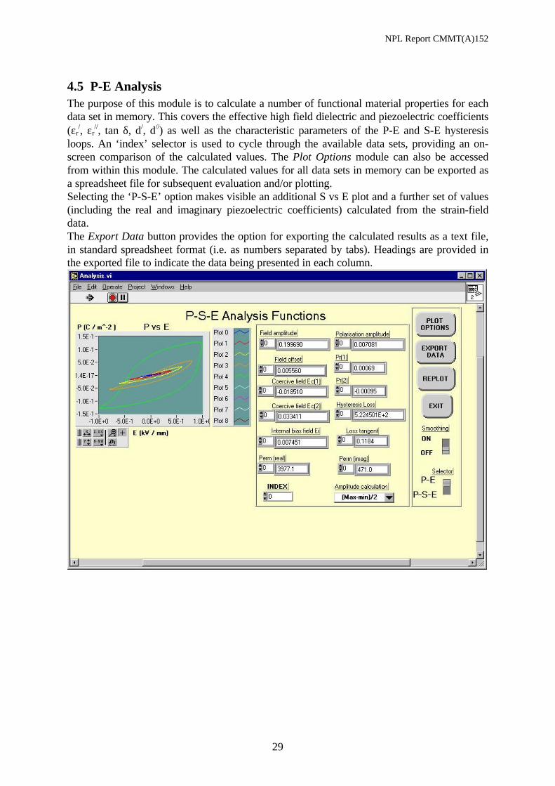
4.5 P-E AnalysisThe purpose of this module is to calculate a number of functional material properties for eachdata set in memory. This covers the effective high field dielectric and piezoelectric coefficients(εr
/, εr//, tan δ, d/, d//) as well as the characteristic parameters of the P-E and S-E hysteresis
loops. An ‘index’ selector is used to cycle through the available data sets, providing an on-screen comparison of the calculated values. The Plot Options module can also be accessedfrom within this module. The calculated values for all data sets in memory can be exported asa spreadsheet file for subsequent evaluation and/or plotting.Selecting the ‘P-S-E’ option makes visible an additional S vs E plot and a further set of values(including the real and imaginary piezoelectric coefficients) calculated from the strain-fielddata.The Export Data button provides the option for exporting the calculated results as a text file,in standard spreadsheet format (i.e. as numbers separated by tabs). Headings are provided inthe exported file to indicate the data being presented in each column.
NPL Report CMMT(A)152
30
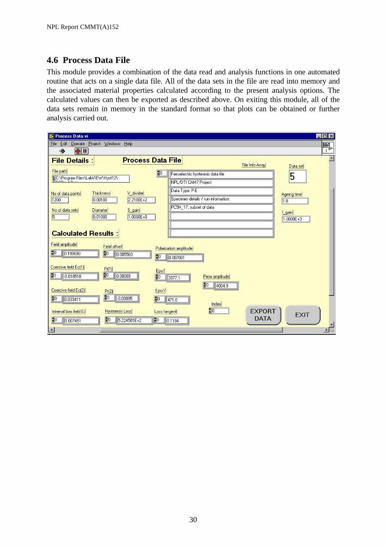
4.6 Process Data FileThis module provides a combination of the data read and analysis functions in one automatedroutine that acts on a single data file. All of the data sets in the file are read into memory andthe associated material properties calculated according to the present analysis options. Thecalculated values can then be exported as described above. On exiting this module, all of thedata sets remain in memory in the standard format so that plots can be obtained or furtheranalysis carried out.

NPL Report CMMT(A)152
31
4.7 Data Acquisition
4.7.1 Main Data Acquisition WindowThe routines for instrument control and data capture are all provided in this module, withinwhich a wide range of instrumentation options and signal characteristics can be set up by theuser. Upon ‘capturing’ a set of waveforms from an A/D card or DSO, the data set can be‘added’ into the memory, where it can then be processed according to all of the actionsdescribed previously. Alternatively, once the required number of data sets has been added tothe memory they can be saved together in a single data file. The memory can then be cleared ifnecessary and further data sets acquired in a similar manner. A routine is also provided forautomatic acquisition of data during an ‘ageing’ experiment.
The data collection in the version of the software provided with this report has been disabledto allow it to run on all machines. Accessing some of the buttons on this menu require datacollection hardware and a message noting this will appear.
The data collection routines have been replaced by the simulation routines discussed earlier.Thus selecting Capture or Trigger and Capture will lead to a screen which enables simulationbased on either the Rayleigh Law or a parallel CR circuit.
The thickness and diameter of the specimen, as well as the number of data points required,should all be entered into the data boxes. Similarly, the current gain and the voltage divider ofthe equipment being used for data acquisition should be entered before any data sets are addedto the memory. The number of data points acquired and the time interval between points arealso indicated here.
Selecting the P-S-E option makes visible further information relating to the field-induceddisplacement data, and an additional plot of the strain-field data.
NPL Report CMMT(A)152
32
4.7.2 Generator Setup**
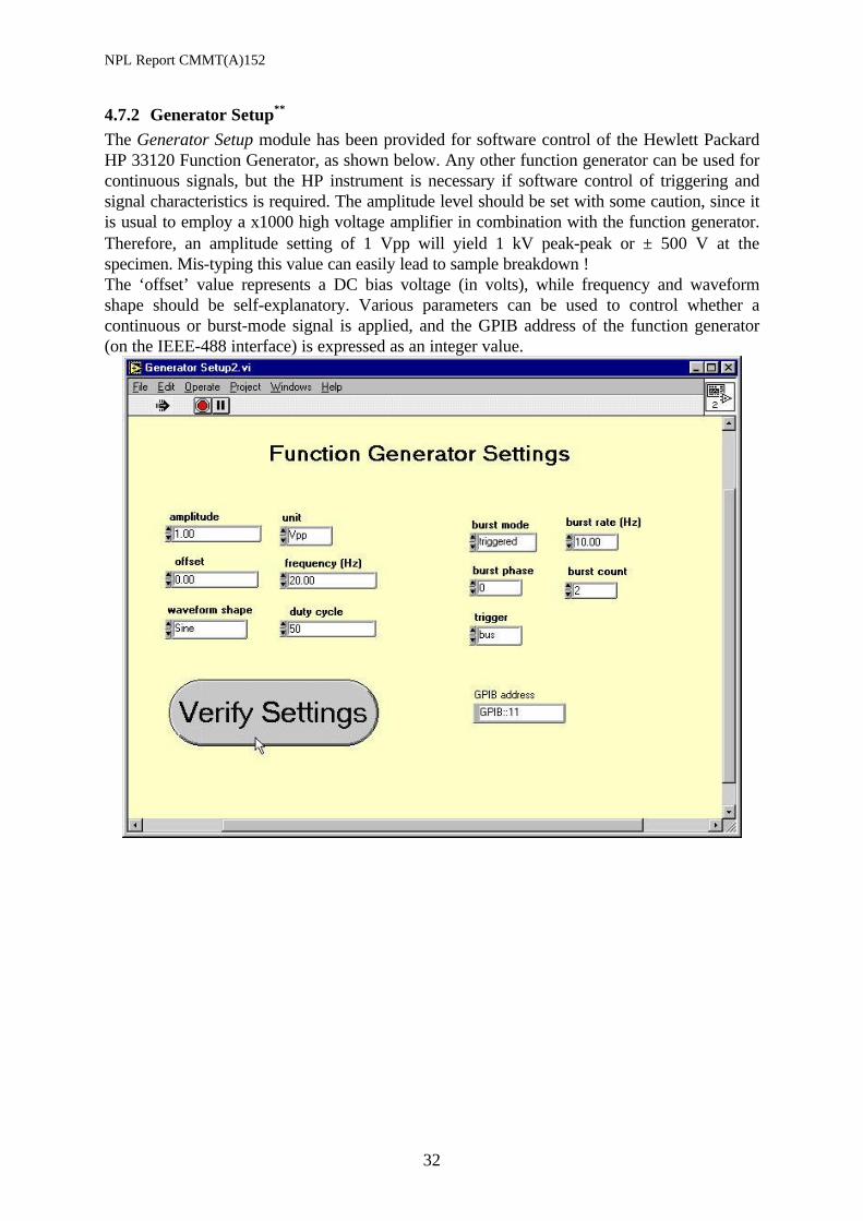
The Generator Setup module has been provided for software control of the Hewlett PackardHP 33120 Function Generator, as shown below. Any other function generator can be used forcontinuous signals, but the HP instrument is necessary if software control of triggering andsignal characteristics is required. The amplitude level should be set with some caution, since itis usual to employ a x1000 high voltage amplifier in combination with the function generator.Therefore, an amplitude setting of 1 Vpp will yield 1 kV peak-peak or ± 500 V at thespecimen. Mis-typing this value can easily lead to sample breakdown !The ‘offset’ value represents a DC bias voltage (in volts), while frequency and waveformshape should be self-explanatory. Various parameters can be used to control whether acontinuous or burst-mode signal is applied, and the GPIB address of the function generator(on the IEEE-488 interface) is expressed as an integer value.
NPL Report CMMT(A)152
33
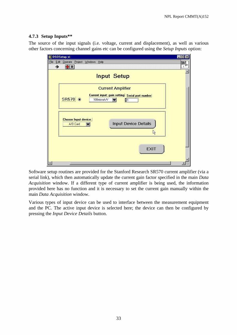
4.7.3 Setup Inputs**The source of the input signals (i.e. voltage, current and displacement), as well as variousother factors concerning channel gains etc can be configured using the Setup Inputs option:
Software setup routines are provided for the Stanford Research SR570 current amplifier (via aserial link), which then automatically update the current gain factor specified in the main DataAcquisition window. If a different type of current amplifier is being used, the informationprovided here has no function and it is necessary to set the current gain manually within themain Data Acquisition window.
Various types of input device can be used to interface between the measurement equipmentand the PC. The active input device is selected here; the device can then be configured bypressing the Input Device Details button.
NPL Report CMMT(A)152
34
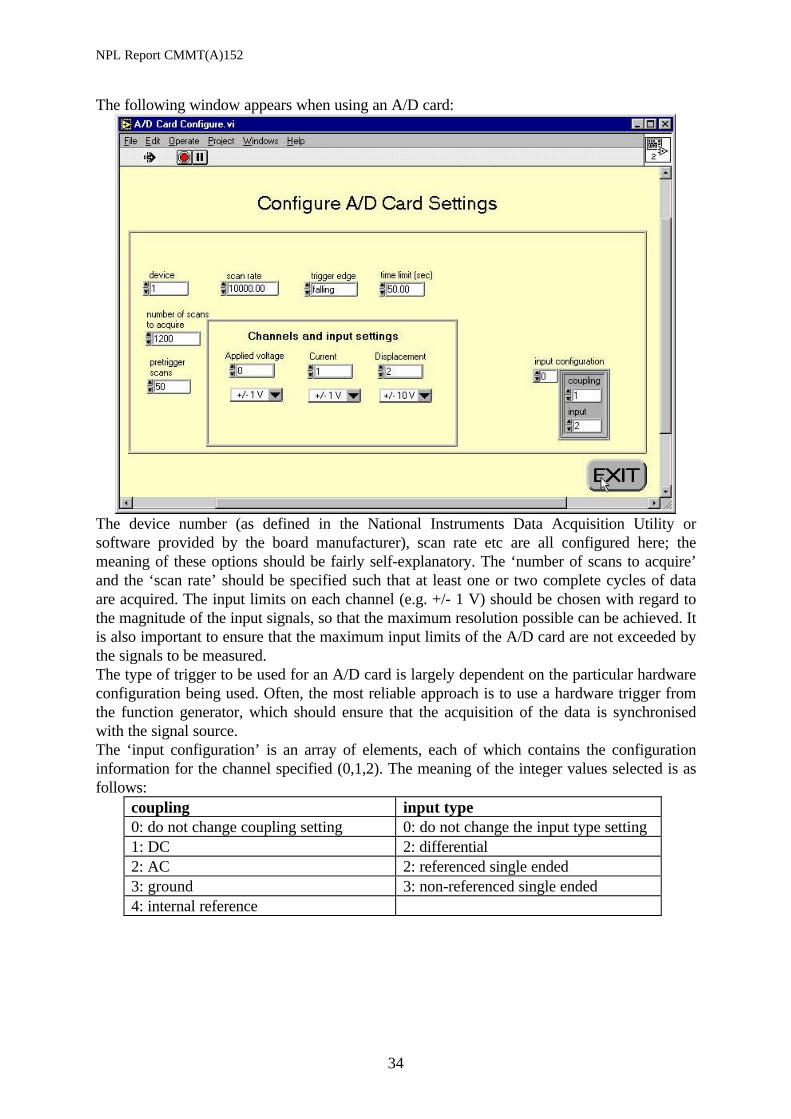
The following window appears when using an A/D card:
The device number (as defined in the National Instruments Data Acquisition Utility orsoftware provided by the board manufacturer), scan rate etc are all configured here; themeaning of these options should be fairly self-explanatory. The ‘number of scans to acquire’and the ‘scan rate’ should be specified such that at least one or two complete cycles of dataare acquired. The input limits on each channel (e.g. +/- 1 V) should be chosen with regard tothe magnitude of the input signals, so that the maximum resolution possible can be achieved. Itis also important to ensure that the maximum input limits of the A/D card are not exceeded bythe signals to be measured.The type of trigger to be used for an A/D card is largely dependent on the particular hardwareconfiguration being used. Often, the most reliable approach is to use a hardware trigger fromthe function generator, which should ensure that the acquisition of the data is synchronisedwith the signal source.The ‘input configuration’ is an array of elements, each of which contains the configurationinformation for the channel specified (0,1,2). The meaning of the integer values selected is asfollows:
coupling input type0: do not change coupling setting 0: do not change the input type setting1: DC 2: differential2: AC 2: referenced single ended3: ground 3: non-referenced single ended4: internal reference
NPL Report CMMT(A)152
35
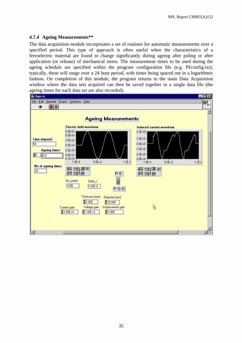
4.7.4 Ageing Measurements**The data acquisition module incorporates a set of routines for automatic measurements over aspecified period. This type of approach is often useful when the characteristics of aferroelectric material are found to change significantly during ageing after poling or afterapplication (or release) of mechanical stress. The measurement times to be used during theageing schedule are specified within the program configuration file (e.g. PEconfig.txt);typically, these will range over a 24 hour period, with times being spaced out in a logarithmicfashion. On completion of this module, the program returns to the main Data Acquisitionwindow where the data sets acquired can then be saved together in a single data file (theageing times for each data set are also recorded).

NPL Report CMMT(A)152
36
4.8 Analysis OptionsCertain options used throughout the program for plotting and analysis of data can be setwithin this module, as illustrated below. The waveform search options specify which datapoints from the electric field waveform are used to construct the I-E, P-E and S-E loops (thesame data points are then also used in the calculation of the effective dielectric andpiezoelectric coefficients). Analysis options include the method of determining the amplitudesof the waveforms (as peak-peak or rms values), the inclusion of strain data, use of datafiltering routines (smoothing) and the reference point for the strain waveform. In addition,correction routines are provided to subtract a parallel conduction current and to correct theapplied voltage signal in the event that a series ‘sense’ resistor is used for measuring theinduced current. The latter correction is not necessary when a ‘virtual earth’ current amplifieris employed (as used throughout the CAM 7 project), but has been used successfully for highfrequency measurements using a sense resistor.
NPL Report CMMT(A)152
37
4.9 Recall / Save SetupAs a whole, the program incorporates a large number of options for data acquisition, plottingand analysis, most of which can be configured by the user within the various modules. Anygiven experimental setup will require customisation of many of these options. It would behighly undesirable if the program required the user to reset these values every time that it wasrun. Therefore, the majority of the options available to the user have been incorporated withina configuration file (default config.txt) which is loaded automatically each time that theprogram is re-started (as described above). A configuration file can be created with theexisting settings simply be selecting the Save Setup action. Also, it is possible to edit aconfiguration file using any word processor, since it is formatted as standard ASCII text.Different program settings can be loaded at any time by choosing the Load Setup action fromthe front panel, which reads in any selected configuration file.
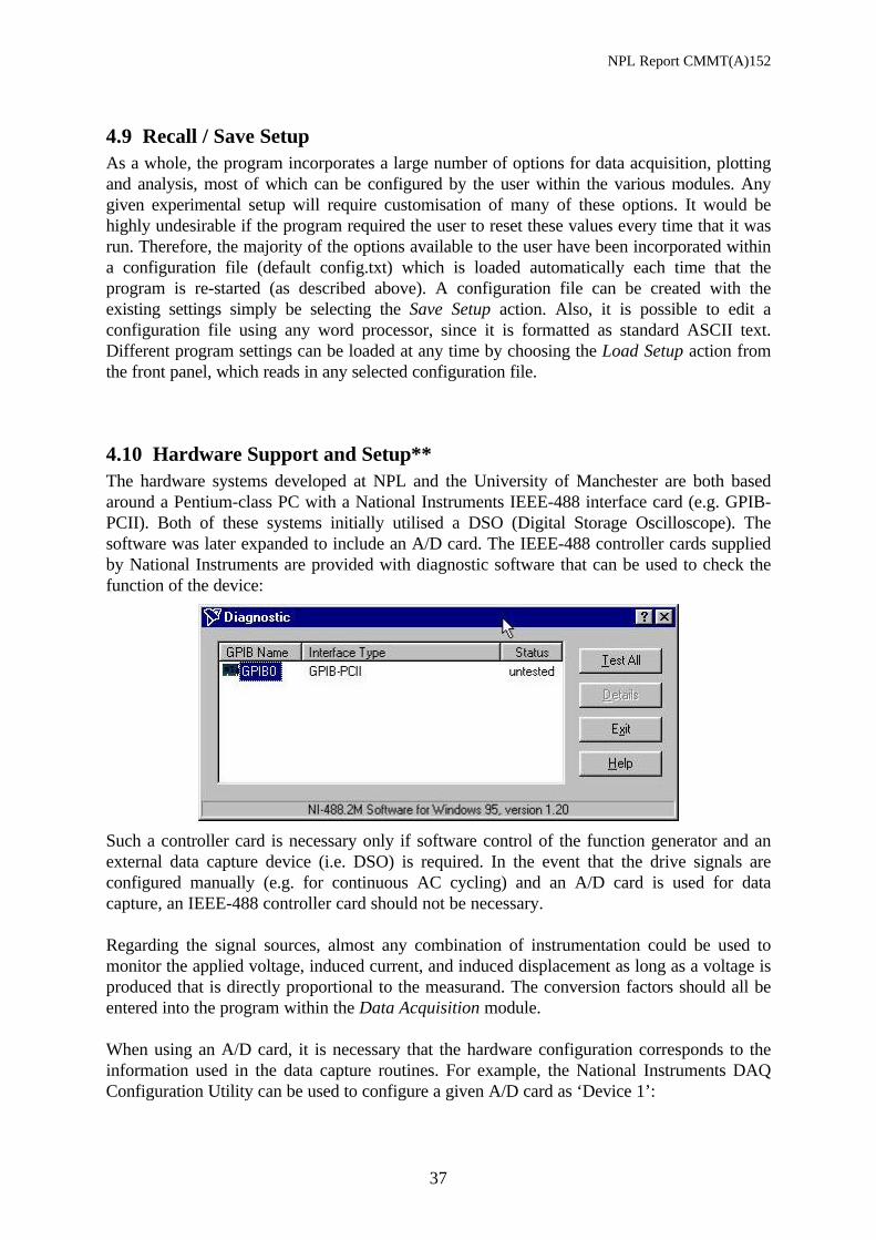
4.10 Hardware Support and Setup**The hardware systems developed at NPL and the University of Manchester are both basedaround a Pentium-class PC with a National Instruments IEEE-488 interface card (e.g. GPIB-PCII). Both of these systems initially utilised a DSO (Digital Storage Oscilloscope). Thesoftware was later expanded to include an A/D card. The IEEE-488 controller cards suppliedby National Instruments are provided with diagnostic software that can be used to check thefunction of the device:
Such a controller card is necessary only if software control of the function generator and anexternal data capture device (i.e. DSO) is required. In the event that the drive signals areconfigured manually (e.g. for continuous AC cycling) and an A/D card is used for datacapture, an IEEE-488 controller card should not be necessary.
Regarding the signal sources, almost any combination of instrumentation could be used tomonitor the applied voltage, induced current, and induced displacement as long as a voltage isproduced that is directly proportional to the measurand. The conversion factors should all beentered into the program within the Data Acquisition module.
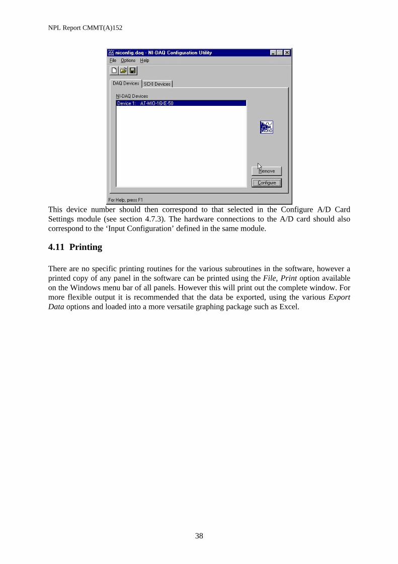
When using an A/D card, it is necessary that the hardware configuration corresponds to theinformation used in the data capture routines. For example, the National Instruments DAQConfiguration Utility can be used to configure a given A/D card as ‘Device 1’:
NPL Report CMMT(A)152
38
This device number should then correspond to that selected in the Configure A/D CardSettings module (see section 4.7.3). The hardware connections to the A/D card should alsocorrespond to the ‘Input Configuration’ defined in the same module.
4.11 Printing
There are no specific printing routines for the various subroutines in the software, however aprinted copy of any panel in the software can be printed using the File, Print option availableon the Windows menu bar of all panels. However this will print out the complete window. Formore flexible output it is recommended that the data be exported, using the various ExportData options and loaded into a more versatile graphing package such as Excel.
NPL Report CMMT(A)152
39
5. References
[1] B Jaffe, W R Cook, and H Jaffe, Piezoelectric Ceramics, New York, Academic Press,1971.
[2] IEEE 180-1986 Standard Definitions of Primary Ferroelectric Terms.[3] J A Main, E Garcia, and D V Newton, Proc. SPIE, 2441, 1995, 243.[4] C B Sawyer and C H Tower, Phys Rev , 35, 1930, 269.[5] H Diamant, K Drenck, and R Pepinsky, Rev Sci Instr, 28, 1957, 30.[6] A M Glazer, P Groves, and D T Smith, J Phys. E, 17, 1984, 95.[7] V R Yarberry and I J Fritz, Rev Sci Instr, 50, 1979, 595.[8] B Dickens, E Balizer, A S DeReggi and S C Roth, J Appl Phys, 72, 1992, 4258.[9] C J Dias and D K Das-Gupta, J Appl Pys, 74, 1993, 6317.[10] D.A. Hall, P.J. Stevenson and T.R. Mullins, Brit. Cer. Proc. 57, 1997, 197-211.
[11] D.A. Hall, M.M. Ben-Omran and P.J. Stevenson, J. Phys: Condensed Matter 10, 1998,461-476.
[12] D.A. Hall and P.J. Stevenson, “High field dielectric properties of ferroelectric ceramics”,Ferroelectrics (in press).
[13] D Jiles, Introduction to Magnetic Materials, Chapman and Hall (1991).
[14] M Demartin and D Damjanovic, Appl. Phys. Lett., 68, 1996, 3046-3048.
[15] Damjanovic and M Demartin, J. Phys. D: Appl. Phys. 29, 1997, 2057-2060.
[16] D Damjanovic, Rep. Prog. Phys. 61, 1998, 1267-1324.

NPL Report CMMT(A)152
40
6. Appendix
6.1 Installing the software
6.1.1 RequirementsThis software has been written and tested on systems running Microsoft Windows 95 andshould be able to run on any PC running Windows 95, although a high specification machine ispreferable. Most of the testing has been done on a 150 MHz Pentium PC and 32 MB of RAM,but it will run satisfactorily on a 100 MHz Pentium with 16 MB RAM. It will not work withWindows 3.1. It has not been fully tested with Windows 98 or Windows NT.
6.1.2 Installing the PEHys softwareThe software should run the main menu when the CD is placed in the drive, and there is anoption on the main menu page to install the software. However should this fail to occur thesoftware can be manually installed using the following procedure.
Use explorer to find the file \disks\setup.exe on the CD-ROM and double click on it, oralternatively use the Start, Run, (CD-ROM drive letter):\disks\setup.exe.The setup program gives the option to install the software anywhere using browse, with thedefault location being C:\Program Files\PEHys. When the location has been chosen pressFinish. The installer will also install the National Instruments Labview Run-Time engine.Should the installation fail before the LabVIEW run-time is installed this component can beseparately installed by running the installation program (CD-ROM driveletter):\disks\RunTime\setup.exe.
6.1.3 Running PEHys softwareThe installation program will set up a program group called NPL PEHys, and the software canbe run by using Start. Programs, PEHys, PEHys.exe.When the program has been started it will display a licence agreement, followed by a requestfor a configuration file, Peconfig.txt. This file is located in the same folder as PEHys.exe. Seethe appendix for the contents of this file and how it affects the software.
6.1.4 Uninstalling the PEHys softwareTo uninstall the NPL PEHys software there are two components that need to be removed,
1) NPL PE loop softwareThere is an uninstall program where the PEHys software is installed. The defaultinstallation occurs in \Program Files\PEHys, so the uninstall program will be \ProgramFiles\PEHys\uninst.exe. Either use Start, Run C: \Program Files\PEHys\uninst.exe orgo to the directory with explorer and double click on uninst.exe. Ignore any messagesregarding erasing read only files and press yes.
2) Labview 5.1 Runtime EngineTo remove this part run Start, Settings, Control Panel, Add/Remove programs andselect NI LabVIEW Run-Time Engine 5.1. Click Add/Remove to remove thissoftware. Removing this software may cause other Labview software not to run, if inany doubt leave this section installed.
NPL Report CMMT(A)152
41
6.2 Some Example files
6.2.1 File: Capb.txtThis file contains 3 PE loops taken at 10, 100 and 500 Hz of a low loss polypropylenecapacitor in parallel with a high voltage resistor. This file can be used to explore the ParallelCR simulation section of the software.
1) Load the software and use “Read Data Files”, “Read New Files”, and choose thefile “capb.txt” which should be in the Data directory.2) There are 3 sets of data in the file (see field “No of data sets in file”), each takenat a different frequency. To select the second curve (100Hz) enter the number 2 inthe field (Which data sets do you require from this file?). And then press OK. Besure not to enter any other characters such as space or carriage return after thenumber or the program will crash. (see troubleshooting).3) Return to the main menu by pressing “Exit” on the Read Data Files subroutine.4) The Data can now be viewed using “Show Plots” or analysed in the “P-EAnalysis” section. If the curves are not displayed see troubleshooting section.5) To calculate simulated P-E loops select “Data Acquisition”.6) Select “Capture”. On the Rayleigh Law or Parallel CR button select Parallel CR.The value of the capacitor can either be set by choosing Capacitance or Permittivity.Choose the Capacitance option and enter the following values, resistance 1.3e+7,capacitance 0.5, voltage 460, frequency 100Hz, and choose sine wave. Press OK toproceed.7) The PE loop should be displayed, and the current-time waveform, however thefield waveform will be a straight line. This is because the acquired waveforms are allon the same full scale and simulates the data seen on an oscilloscope screen. Toexpand the data experiment by changing the current gain from 1e+6 to 1e+3, andrepeating the “Capture” process above. The field and current waveforms shouldnow both be visible. The strain waveform will now be visible as a straight line. Thisis because there is no strain channel in the Parallel CR simulation. Switch the P-E P-S-E button to P-E, and repeat the capture process. There should now only be twowaveforms present, field and current.8) There should be one data set in memory (the experimental data loaded fromcapb.txt). Press “Add data to memory” to store the simulated data, and the no ofdata sets in memory should rise to 2.9) Press “exit” to return to the main menu.10) The Data can now be viewed using “Show Plots” or analysed in the “P-EAnalysis”. The two curves, simulated (red) and experimental (blue) should bealmost identical.11) This process can now be repeated for the 10Hz case, either by adding onto thetwo PE loops stored in memory, or by clearing the memory and starting again.12) To clear memory select, “Read Data Files”, “Clear Data”.13) To examine the 10Hz data, load curve number 3 from capb.txt, and to createsimulated data use the identical settings in step 6 except using a frequency of 10Hz.
NPL Report CMMT(A)152
42
6.2.2 File: PC5H_13.hyz
This file contains a series of 30 PE loops obtained experimentally on a PC 5H material alltaken at 1Hz, with fields increasing from 0.05 to 3.5kV/mm. This file can be used toinvestigate the Rayleigh law simulation subroutine of the software and examine how thebehaviour deviates from the Rayleigh law at high fields.
1) Load the software and use “Read Data Files”, “Read New Files”, and choose thefile “pc5H_13.hyz” which should be in the Data directory.2) There are 30 sets of data in the file (see field “No of data sets in file”), taken atincreasing voltages. Select the ninth curve (400volts) enter the number 9 in thefield (Which data sets do you require from this file?). And then press OK. Be surenot to enter any other characters such as space or carriage return after the numberor the program will crash. (see troubleshooting).3) Return to the main menu by pressing “Exit” on the Read Data Files subroutine.4) The Data can now be viewed using “Show Plots” or analysed in the “P-EAnalysis” section. If the curves are not displayed see troubleshooting section.5) To calculate simulated P-E loops select “Data Acquisition”.6) Select “Capture”. On the Rayleigh Law or Parallel CR button select RayleighLaw. Enter the following values, relative permittivity 3030, alpha 7e-3, voltage 400,frequency 1Hz, and choose sine wave. We are not interested in the strain channel soleave the d33 at 600 and d33 alpha at 0. Press OK to proceed.7) The PE loop should be displayed, the current-time waveform, however the fieldand strain waveform will be comparatively small. This is because the acquiredwaveforms are all on the same full scale and simulates the data seen on anoscilloscope screen. To expand the data experiment by changing the current gainfrom 1e+6 to 1e+5, and hide the strain data by switching the P-E P-S-E button toP-E. Then repeat the “Capture” process above. The field and current waveformsshould now both be visible.8) There should be one data set in memory (the experimental data loaded frompc5H_13.hyz). Press “Add data to memory” to store the simulated data, and the noof data sets in memory should rise to 2.9) Press “exit” to return to the main menu.10) The Data can now be viewed using “Show Plots” or analysed in the “P-EAnalysis”. The two curves, simulated (red) and experimental (blue) should bealmost identical. On close examination of the current time curves there is reasonableagreement on the positive voltage side, but there is a larger deviation on thenegative going cycle. This is because the experimental data comes from a poledsample which has a directionality. The Rayleigh law will always predict symmetricalnegative and positive behaviour.11) This process can now be repeated for the lower and higher field curves, either byadding onto the two PE loops stored in memory, or by clearing the memory andstarting again.12) To clear memory select, “Read Data Files”, “Clear Data”.13) To examine more data use “Read Data Files”, “Read New Data”.
NPL Report CMMT(A)152
43
6.2.3 File: Rayleigh.txt
This file contains some simulated PSE data obtained using the current PE loop software andsaving the data as if it were experimental curves. The data simulated is at 100Hz on a 10mmdiameter 1mm thick disc, with the Rayleigh law parameters permittivity=3000, aplha=5.0e-3,d33=600 and d33 alpha=5.0e-4. There are 5 loops at voltages from 200 to 1000 volts. The filecan be used to investigate the analysis routine in more detail, and the effect of d33 alpha on thepiezoelectric coefficient and piezoelectric loss tangent.
1) Load the software and use “Read Data Files”, “Read New Files”, and choose thefile “rayleigh.txt” which should be in the Data directory.2) There are 5 sets of data in the file (see field “No of data sets in file”), taken atincreasing voltages. Select all the curves, enter the number 1 2 3 4 5 in the field(Which data sets do you require from this file?). And then press OK. Be sure toseparate each number with a space and not to enter any other characters such asspace or carriage return after the last number or the program will crash. (seetroubleshooting).3) Return to the main menu by pressing “Exit” on the Read Data Files subroutine.4) The Data can now be analysed in the “P-E Analysis” section.5) If the curves are not displayed see troubleshooting section.6) To view the results for the individual curves change the index number, either bypressing the up and down arrow, or by entering a number. All the parameters forthe PE loop will be displayed. Careful that this index starts at zero, so PE loop 1will have an index of 0, and for 5 curves the last index is 4. For a value of indexgreater than the number of PE loops all the parameter boxes will be ‘greyed out’.7) The parameters for all five PE loops can be saved for retrieval into say aspreadsheet by selecting “Export Data” button. The data is in ASCII text format.8) The effect of using RMS rather than peak to peak values can be investigating byselecting this option. In order for the changed option to come into effect the“Replot” button must be pressed after each change. If the data is exported for eachcase the differences can be quantified. Similarly the effect of data smoothing can beinvestigated by selecting “Plot Options” to change the data smoothing parameters.
6.3 File Formats
6.3.1 Configuration File : Peconfig.txtThe following file listing is the peconfig.txt file that comes with the PEHys software, shouldany changes be accidentally made to the file causing errors this version, found on the CDshould return normal operation. The configuration file is broken down into several sections,some of which have little or no effect on the operation of the hardware control disabledversion supplied with this report.
New versions of this file can be created by using the “Save Setup” command from the mainmenu, and loaded using “Recall Setup”. There is limited error checking on loading this file soerrors in the file may not be immediately obvious until unexpected results occur in the output.
*** DATA ACQUISITION OPTIONS ***

NPL Report CMMT(A)152
44
All the items prior to Serial port in this section will affect the operation of the software. Acommon mistake is to load a file other than peconfig.txt which may lead to gains of zero, andnumber of points acquired zero. This will only affect the data acquisition section of thesoftware and should not affect the loading previously saved of data files and subsequentplotting and analysis.
The Ageing measurement times is used to automatically capture P-S-E loops at a series offixed times. This will not work in the hardware disabled version.
*** FUNCTION GENERATOR OPTIONS ***This section deals with data capture using a function generator to generate the applied voltagesignal and has no affect on operation of the hardware disabled version.
*** SMOOTHING/FILTERING OPTIONS ***These section affects the values in the “Filter Options” sub section of “Plot Options” in either“P-E Analysis” or “Show Plots”. These will only effect the data if the smoothing option hasbeen selected, either by switching the button or having the value TRUE in Waveformsmoothing (boolean):.
*** PLOTTING/ANALYSIS OPTIONSThese values affect the way the zero crossover is found in order to identify a single hysteresisloop, and also switch on the correction factors for using a sense resistor to measure current.These options can be accessed either through “Analysis Options” on the main menu or the“Plot Options” sub menu of either “P-E Analysis” or “Show Plots.
****** DATA READ OPTIONS ***The contents of this section can change the operation of the current version. Obviously thenumber of data sets and points should not be less than the data files that are being loaded orcaptured. These number affect the amount of memory needed for the program to store data,and can be reduced if the program reports memory errors, although obviously the amount ofdata allowed will be reduced.
*** A/D Card Options ***This section deals with data capture using a National Instruments A/D card and has no effecton operation of the hardware disabled version.
PEHys Configuration FileNPL/DTI CAM7 Project
*** DATA ACQUISITION OPTIONS ***Number of points required:1200Voltage divider:1.000000E+3Displacement gain (Volts/micron):1.000000E+0Current gain (Volts/amp):
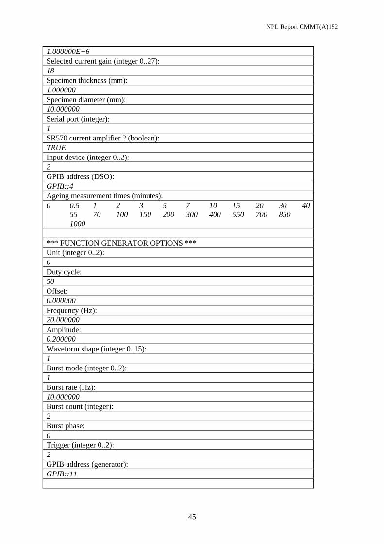
NPL Report CMMT(A)152
45
1.000000E+6Selected current gain (integer 0..27):18Specimen thickness (mm):1.000000Specimen diameter (mm):10.000000Serial port (integer):1SR570 current amplifier ? (boolean):TRUEInput device (integer 0..2):2GPIB address (DSO):GPIB::4Ageing measurement times (minutes):0 0.5 1 2 3 5 7 10 15 20 30 40
55 70 100 150 200 300 400 550 700 8501000
*** FUNCTION GENERATOR OPTIONS ***Unit (integer 0..2):0Duty cycle:50Offset:0.000000Frequency (Hz):20.000000Amplitude:0.200000Waveform shape (integer 0..15):1Burst mode (integer 0..2):1Burst rate (Hz):10.000000Burst count (integer):2Burst phase:0Trigger (integer 0..2):2GPIB address (generator):GPIB::11

NPL Report CMMT(A)152
46
*** SMOOTHING/FILTERING OPTIONS ***Waveform smoothing (boolean):FALSEFilter Rank (integer for averaging routine):6Select filter type (integer 0..1):0Windowed filter type (integer 0..3):0Window (integer 0..8):1Number of taps (integer):50Pass frequency (Hz):200.000000Stop frequency (Hz):1000.000000Sampling frequency (Hz):1000.000000
*** PLOTTING/ANALYSIS OPTIONS ***Threshold value (%):1.000000Start search (integer):0Sense resistor correction (boolean):FALSEConduction correction (boolean):FALSEPlot type (integer 0..7):0Start zero (integer):1End zero (integer):3Find amplitude switch (integer 0..1):0PE/PSE switch (boolean):FALSE
*** DATA READ OPTIONS ***Maximum number of data sets (integer):30Maximum number of points (integer):2500Maximum number of zeros (integer):

NPL Report CMMT(A)152
47
30Strain zero analysis option (boolean):TRUE
*** A/D Card Options ***Device number (integer):1Pretrigger Scans (integer):0Trigger edge (integer 0..2):2Time limit / s (real):50.000000Applied voltage channel (integer):0Voltage channel limits (integer 0..3):3Induced current channel (integer):1current channel limits (integer 0..3):3induced strain channel (integer):2strain channel limits (integer 0..3):3Input configuration definition Channel0 (Coupling, input):1 2Input configuration definition Channel1 (Coupling, input):1 2Input configuration definition Channel2 (Coupling, input):1 2Number of scans to acquire (integer):1200Scan rate (per second):5000.000000
6.3.2 P-E and P-S-E Data Files
The format for the data files is ASCII text and the contents of each line are given below. Thefile names can have any extension name, but it is convenient to call them .txt so that they canbe viewed easily with Notepad or WordPad in Windows95. P-E files are purely field andcurrent data, whereas P-S-E files also include the strain channel.
P-E Data Files
Line1 Ferroelectric hysteresis data file (+version details)

NPL Report CMMT(A)152
48
2 NPL/DTI CAM7 project3 Data Type: P-E4 Specimen details / run information:5 Info line 16 Info line 27 Info line 38 Info line 49 Specimen geometry (thickness and diameter / m):10 Thick Diam11 Generator details (frequency, wave, burst mode):12 frequency wave type burst/continuous13 Filter details:14 Low pass High pass15 Number of data sets and number of points per set:16 No_sets No_points17 Data:18 Set[1] Age_time[1] Current_gain[1] Volts_gain[1]19 t[1,1] Volts_E[1,1] Volts_I[1,1]20 t[1,2] Volts_E[1,2] Volts_I[1,2]21 .22 .. t[1,N] Volts_E[1,N] Volts_I[1,N]. Set[2] Age_time[2] Volts_gain[2] Current_gain[2]. t[2,1] Volts_E[2,1] Volts_I[2,1]. t[2,2] Volts_E[2,2] Volts_I[2,2]. .P-S-E Data FilesLine1 Ferroelectric hysteresis data file (+version details)2 NPL/DTI CAM7 project3 Data Type: P-S-E4 Specimen details / run information:5 Info line 16 Info line 27 Info line 38 Info line 49 Specimen geometry (thickness and diameter / m):10 Thick Diam11 Generator details (frequency, wave, burst mode):12 frequency wave type burst/continuous13 Filter details:14 Low pass High pass15 Number of data sets and number of points per set:16 No_sets No_points17 Data:18 Set[1] Age_time[1] Current_gain[1] Volts_gain[1] Strain_gain[1]

NPL Report CMMT(A)152
49
19 t[1,1] Volts_E[1,1] Volts_I[1,1] Volts_S[1,1]. t[1,2] Volts_E[1,2] Volts_I[1,2] Volts_S[1,2]. .. .. t[1,N] Volts_E[1,N] Volts_I[1,N] Volts_S[1,N]. Set[2] Age_time[2] Volts_gain[2] Current_gain[2] Strain_gain[2]. t[2,1] Volts_E[2,1] Volts_I[2,1] Volts_S[2,1]
t[2,2] Volts_E[2,2] Volts_I[2,2] Volts_S[2,2]. .. .
6.4 Troubleshooting
Unable to locate the LabVIEW runtime engine?The Labview runtime engine has not been properly installed during the installation. Thiscomponent can be separately installed by running the setup program in the disks\RunTimedirectory on the CD.
Program hangs when I close a window?It is possible to exit individual windows using the normal windows exit modes such as clickingon the x in the right hand corner. However if this is done while the program is expecting inputwithin this window then it is impossible to continue. To prevent this the user should exit eachsubmenu using the required continuation button, usually Exit. To recover from this conditionthe user will need to exit the program, by clicking File, Exit, and then restart the program.
Program hangs when loading data from a file?When loading files using the “Read New Files” subroutine be sure not to enter any othercharacters after the final number. A list of numbers should be entered in increasing numericalorder separated by spaces, but characters such as space or carriage return after the finalcharacter will cause an endless loop. Decreasing numerical sequences will also cause the sameendless loop. The Data set being read will keep increasing endlessly. The user will need to exitthe program, by clicking File, Exit, and then restart the program.
Incorrect results for different sample sizes?The data structure for the saved files is such that the sample dimensions are held at thebeginning of the file and all the rest of the data in the file will implicitly be assigned the samedimensions. Therefor although it is possible to mix results from different samples in one file,this will lead to incorrect results if they are of different dimensions.
No curves or only partial curves on graph?Sometimes the scaling on the graphs may not display the curve correctly. The simplest way toreset the scaling is to press the buttons marked X and Y underneath the graph in question. Thegraph can also be zoomed using the magnifying glass button, and moved by using the handbutton.
No curves on graph?

NPL Report CMMT(A)152
50
A common mistake is to forget to click “Add data to memory” after data capture. The Dataacquisition will always display the last data set captured, but this has to be added to memoryfor use in the rest of the program. The number of data sets in memory should increase by onewhen the “add data to memory button” is pressed.
Strange results when doing data capture/simulation?The configuration file peconfig.txt is a text file containing information such as current gain,voltage gain etc, which is loaded at the beginning of the program. There is limited errorchecking on this file and it is possible to load any file at this point, and the software will usewhatever settings it determines from this file. This is indicated by current gains of zero, andnumber of points required 0. To reload the correct configuration select “recall setup” on themain menu, and load the file Peconfig.txt. If this file has been corrupted by accidentally savingwith “save setup”, then reload the original peconfig.txt data file from the data directory on theCD.
Memory Full Problems?Try closing down any other applications that you may have running. Decrease the amount ofdata loaded by reducing the number of curves loaded simultaneously, and reduce the size ofsimulated data by reducing the number of points required.

NPL Report CMMT(A)152
51
6.5 Restrictions and Copyright
6.5.1 Version 1.9 CD releaseThis software was designed and developed by David Hall at the University of Manchester, andMark Stewart at the National Physical Laboratory as part of the UK DTI funded projectCAM7. In this version the hardware control subroutines have been disabled and replaced bysimulated data. If you are interested in the version with hardware control please contact theauthors at NPL.
6.5.2 Licence Agreement
This demonstration Software is provided AS IS and without any warranty. You may installthis copy of the Software on a stand-alone machine or on a network and use it freely forevaluation purposes.
The demonstration Software is owned by the National Physical Laboratory (UK). All Softwareare protected by English law and international treaty provisions.
You may not copy any written material provided with the Software. You may not rent, lease,sublicense, transfer, sell or resell the Software. You may not reverse engineer, decompile, ordisassemble the Software.
To the maximum extent permitted by applicable law, in no event shall the owners of theSoftware or their suppliers be liable for any damages whatsoever (including, withoutlimitation, damages for loss of business profits, business interruption, loss of businessinformation, or other pecuniary loss) arising out of the use or inability to use the Software.
This software has not been fully subjected to NPL's Quality Assurance procedures. Nowarranty or guarantee applies to this software, and therefore any users should satisfythemselves that it meets their requirements.
This application has been built using Labview. Copyright © 1999 National InstrumentsCorporation. All Rights Reserved. ** The hardware control subroutines in this version have been disabled, so the following section may notfunction as described, however these notes have been left to summarise the full version.