feedback fundamentals - caltech computingmurray/courses/cds101/fa02/caltech/a... · ration of the...

5

Feedback Fundamentals

5.1 Introduction

Fundamental properties of feedback systems will be investigated in thisChapter. We begin in Section 5.2 by discussing the basic feedback loop andtypical requirements. This includes the ability to follow reference signals,effects of load disturbances and measurement noise and the effects of pro-cess variations. It turns out that these properties can be captured by aset of six transfer functions, called the Gang of Six. These transfer func-tions are introduced in Section 5.3. For systems where the feedback isrestricted to operate on the error signal the properties are characterizedby a subset of four transfer functions, called the Gang of Four. Propertiesof systems with error feedback and the more general feedback configura-tion with two degrees of freedom are also discussed in Section 5.3. It isshown that it is important to consider all transfer functions of the Gangof Six when evaluating a control system. Another interesting observationis that for systems with two degrees of freedom the problem of responseto load disturbances can be treated separately. This gives a natural sepa-ration of the design problem into a design of a feedback and a feedforwardsystem. The feedback handles process uncertainties and disturbances andthe feedforward gives the desired response to reference signals.

Attenuation of disturbances are discussed in Section 5.4 where it isdemonstrated that process disturbances can be attenuated by feedbackbut that feedback also feeds measurement noise into the system. It turnsout that the sensitivity function which belongs to the Gang of Four givesa nice characterization of disturbance attenuation. The effects of processvariations are discussed in Section 5.5. It is shown that their effects arewell described by the sensitivity function and the complementary sensi-tivity function. The analysis also gives a good explanation for the fact that

177

Richard Murray

From _Control System Design_ by Karl Johan Åström, 2002

Richard Murray

Copyright 2002, Karl Johan Åström. All rights reserved. Do not duplicate or redistribute.

Chapter 5. Feedback Fundamentals

F C P

−1

Σ Σ Σr e u v

d

x

n

y

Controller Process

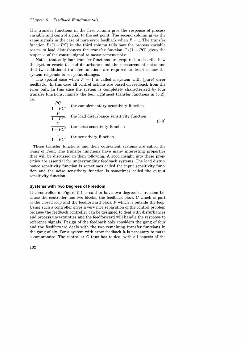
Figure 5.1 Block diagram of a basic feedback loop.

control systems can be designed based on simplified models. When dis-cussing process variations it is natural to investigate when two processesare similar from the point of view of control. This important nontrivialproblem is discussed in Section 5.6. Section 5.7 is devoted to a detailedtreatment of the sensitivity functions. This leads to a deeper understand-ing of attenuation of disturbances and effects of process variations. Afundamental result of Bode which gives insight into fundamental limi-tations of feedback is also derived. This result shows that disturbancesof some frequencies can be attenuated only if disturbances of other fre-quencies are amplified. Tracking of reference signals are investigated inSection 5.8. Particular emphasis is given to precise tracking of low fre-quency signals. Because of the richness of control systems the emphasison different issues varies from field to field. This is illustrated in Sec-tion 5.10 where we discuss the classical problem of design of feedbackamplifiers.

5.2 The Basic Feedback Loop

A block diagram of a basic feedback loop is shown in Figure 5.1. The sys-tem loop is composed of two components, the process P and the controller.The controller has two blocks the feedback block C and the feedforwardblock F. There are two disturbances acting on the process, the load distur-bance d and the measurement noise n. The load disturbance representsdisturbances that drive the process away from its desired behavior. Theprocess variable x is the real physical variable that we want to control.Control is based on the measured signal y, where the measurements arecorrupted by measurement noise n. Information about the process variablex is thus distorted by the measurement noise. The process is influencedby the controller via the control variable u. The process is thus a systemwith three inputs and one output. The inputs are: the control variable

178

5.2 The Basic Feedback Loop

C

P yuzw

Figure 5.2 An abstract representation of the system in Figure 5.1. The input urepresents the control signal and the input w represents the reference r, the loaddisturbance d and the measurement noise n. The output y is the measured variablesand z are internal variables that are of interest.

u, the load disturbance d and the measurement noise n. The output isthe measured signal. The controller is a system with two inputs and oneoutput. The inputs are the measured signal y and the reference signal rand the output is the control signal u. Note that the control signal u is aninput to the process and the output of the controller and that the mea-sured signal is the output of the process and an input to the controller. InFigure 5.1 the load disturbance was assumed to act on the process input.This is a simplification, in reality the disturbance can enter the processin many different ways. To avoid making the presentation unnecessar-ily complicated we will use the simple representation in Figure 5.1. Thiscaptures the essence and it can easily be modified if it is known preciselyhow disturbances enter the system.

More Abstract Representations

The block diagrams themselves are substantial abstractions but higherabstractions are sometimes useful. The system in Figure 5.1 can be rep-resented by only two blocks as shown in Figure 5.2. There are two typesof inputs, the control u, which can be manipulated and the disturbancesw = (r, d, n), which represents external influences on the closed loopsystems. The outputs are also of two types the measured signal y andother interesting signals z = (e, v, x). The representation in Figure 5.2allows many control variables and many measured variables, but it showsless of the system structure than Figure 5.1. This representation can beused even when there are many input signals and many output signals.Representation with a higher level of abstraction are useful for the devel-opment of theory because they make it possible to focus on fundamentalsand to solve general problems with a wide range of applications. Caremust, however, be exercised to maintain the coupling to the real worldcontrol problems we intend to solve.

179


Disturbances

Attenuation of load disturbances is often a primary goal for control. This isparticularly the case when controlling processes that run in steady state.Load disturbances are typically dominated by low frequencies. Considerfor example the cruise control system for a car, where the disturbances arethe gravity forces caused by changes of the slope of the road. These distur-bances vary slowly because the slope changes slowly when you drive alonga road. Step signals or ramp signals are commonly used as prototypes forload disturbances disturbances.

Measurement noise corrupts the information about the process vari-able that the sensors delivers. Measurement noise typically has high fre-quencies. The average value of the noise is typically zero. If this was notthe case the sensor will give very misleading information about the pro-cess and it would not be possible to control it well. There may also bedynamics in the sensor. Several sensors are often used. A common situa-tion is that very accurate values may be obtained with sensors with slowdynamics and that rapid but less accurate information can be obtainedfrom other sensors.

Actuation

The process is influenced by actuators which typically are valves, motors,that are driven electrically, pneumatically, or hydraulically. There are of-ten local feedback loops and the control signals can also be the referencevariables for these loops. A typical case is a flow loop where a valve iscontrolled by measuring the flow. If the feedback loop for controlling theflow is fast we can consider the set point of this loop which is the flowas the control variable. In such cases the use of local feedback loops canthus simplify the system significantly. When the dynamics of the actua-tors is significant it is convenient to lump them with the dynamics of theprocess. There are cases where the dynamics of the actuator dominatesprocess dynamics.

Design Issues

Many issues have to be considered in analysis and design of control sys-tems. Basic requirements are

• Stability

• Ability to follow reference signals

• Reduction of effects of load disturbances

• Reduction of effects of measurement noise

• Reduction of effects of model uncertainties

180

5.3 The Gang of Six

The possibility of instabilities is the primary drawback of feedback. Avoid-ing instability is thus a primary goal. It is also desirable that the processvariable follows the reference signal faithfully. The system should alsobe able to reduce the effect of load disturbances. Measurement noise isinjected into the system by the feedback. This is unavoidable but it is es-sential that not too much noise is injected. It must also be considered thatthe models used to design the control systems are inaccurate. The proper-ties of the process may also change. The control system should be able tocope with moderate changes. The focus on different abilities vary with theapplication. In process control the major emphasis is often on attenuationof load disturbances, while the ability to follow reference signals is theprimary concern in motion control systems.

5.3 The Gang of Six

The feedback loop in Figure 5.1 is influenced by three external signals,the reference r, the load disturbance d and the measurement noise n.There are at least three signals x, y and u that are of great interestfor control. This means that there are nine relations between the inputand the output signals. Since the system is linear these relations can beexpressed in terms of the transfer functions. Let X , Y, U , D, N R be theLaplace transforms of x, y, u, d, n r, respectively. The following relationsare obtained from the block diagram in Figure 5.1

X = P1+ PC

D − PC1+ PC

N + PCF1+ PC

R

Y = P1+ PC

D + 11+ PC

N + PCF1+ PC

R

U = − PC1+ PC

D − C1+ PC

N + CF1+ PC

R.

(5.1)

To simplify notations we have dropped the arguments of all Laplace trans-forms. There are several interesting conclusions we can draw from theseequations. First we can observe that several transfer functions are thesame and that all relations are given by the following set of six transferfunctions which we call the Gang of Six.

PCF1+ PC

PC1+ PC

P1+ PC

CF1+ PC

C1+ PC

11+ PC

,(5.2)

181


The transfer functions in the first column give the response of processvariable and control signal to the set point. The second column gives thesame signals in the case of pure error feedback when F = 1. The transferfunction P/(1 + PC) in the third column tells how the process variablereacts to load disturbances the transfer function C/(1 + PC) gives theresponse of the control signal to measurement noise.

Notice that only four transfer functions are required to describe howthe system reacts to load disturbance and the measurement noise andthat two additional transfer functions are required to describe how thesystem responds to set point changes.

The special case when F = 1 is called a system with (pure) errorfeedback. In this case all control actions are based on feedback from theerror only. In this case the system is completely characterized by fourtransfer functions, namely the four rightmost transfer functions in (5.2),i.e.

PC1+ PC

, the complementary sensitivity function

P1+ PC

, the load disturbance sensitivity function

C1+ PC

, the noise sensitivity function

11+ PC

, the sensitivity function

(5.3)

These transfer functions and their equivalent systems are called theGang of Four. The transfer functions have many interesting propertiesthat will be discussed in then following. A good insight into these prop-erties are essential for understanding feedback systems. The load distur-bance sensitivity function is sometimes called the input sensitivity func-tion and the noise sensitivity function is sometimes called the outputsensitivity function.

Systems with Two Degrees of Freedom

The controller in Figure 5.1 is said to have two degrees of freedom be-cause the controller has two blocks, the feedback block C which is partof the closed loop and the feedforward block F which is outside the loop.Using such a controller gives a very nice separation of the control problembecause the feedback controller can be designed to deal with disturbancesand process uncertainties and the feedforward will handle the response toreference signals. Design of the feedback only considers the gang of fourand the feedforward deals with the two remaining transfer functions inthe gang of six. For a system with error feedback it is necessary to makea compromise. The controller C thus has to deal with all aspects of the

182

5.3 The Gang of Six

0 10 20 30

0

0.5

1

1.5

0 10 20 30

0

0.5

1

1.5

0 10 20 30

0

0.5

1

1.5

0 10 20 30

0

0.5

1

1.5

0 10 20 30

0

0.5

1

1.5

0 10 20 30

0

0.5

1

1.5

PCF/(1 + PC) PC/(1+ PC)

C/(1+ PC)

P/(1 + PC)

CF/(1+ PC) 1/(1+ PC)

Figure 5.3 Step responses of the Gang of Six for PI control k = 0.775, Ti = 2.05of the process P(s) = (s + 1)−4. The feedforward is designed to give the transferfunction (0.5s+ 1)−4 from reference r to output y.

problem.To describe the system properly it is thus necessary to show the re-

sponse of all six transfer functions. The transfer functions can be repre-sented in different ways, by their step responses and frequency responses,see Figures 5.3 and 5.4.

Figures 5.3 and 5.4 give useful insight into the properties of the closedloop system. The time responses in Figure 5.3 show that the feedforwardgives a substantial improvement of the response speed. The settling timeis substantially shorter, 4 s versus 25 s, and there is no overshoot. This isalso reflected in the frequency responses in Figure 5.4 which shows thatthe transfer function with feedforward has higher bandwidth and that ithas no resonance peak.

The transfer functions CF/(1 + PC) and −C/(1 + PC) represent thesignal transmission from reference to control and from measurement noiseto control. The time responses in Figure 5.3 show that the reduction inresponse time by feedforward requires a substantial control effort. Theinitial value of the control signal is out of scale in Figure 5.3 but thefrequency response in 5.4 shows that the high frequency gain of PCF/(1+PC) is 16, which can be compared with the value 0.78 for the transferfunction C/(1+ PC). The fast response thus requires significantly largercontrol signals.

There are many other interesting conclusions that can be drawn fromFigures 5.3 and 5.4. Consider for example the response of the output to

183


10−1

100

101

10−1

100

10−1

100

101

10−1

100

10−1

100

101

10−1

100

10−1

100

101

100

101

10−1

100

101

100

101

10−1

100

101

100

101

PCF/(1 + PC) PC/(1+ PC)

C/(1+ PC)

P/(1 + PC)

CF/(1+ PC) 1/(1+ PC)

Figure 5.4 Gain curves of frequency responses of the Gang of Six for PI controlk = 0.775, Ti = 2.05 of the process P(s) = (s+1)−4 where the feedforward has beendesigned to give the transfer function (0.5s+ 1)−4 from reference to output.

load disturbances expressed by the transfer function P/(1 + PC). Thefrequency response has a pronounced peak 1.22 at ω max = 0.5 the corre-sponding time function has its maximum 0.59 at tmax = 5.2. Notice thatthe peaks are of the same magnitude and that the product of ω maxtmax =2.6.

The step responses can also be represented by two simulations of theprocess. The complete system is first simulated with the full two-degree-of-freedom structure. The simulation begins with a step in the referencesignal, when the system has settled to equilibrium a step in the load dis-turbance is then given. The process output and the control signals arerecorded. The simulation is then repeated with a system without feedfor-ward, i.e. F = 1. The response to the reference signal will be differentbut the response to the load disturbance will be the same as in the firstsimulation. The procedure is illustrated in Figure 5.5.

A Remark

The fact that 6 relations are required to capture properties of the basicfeedback loop is often neglected in literature. Most papers on control onlyshow the response of the process variable to set point changes. Such acurve gives only partial information about the behavior of the system. Toget a more complete representation of the system all six responses shouldbe given. We illustrate the importance of this by an example.

184

5.3 The Gang of Six

0 10 20 30 40 50 600

0.5

1

1.5

2Process variable

0 10 20 30 40 50 60−0.5

0

0.5

1

1.5Control signal

Figure 5.5 Representation of properties of a basic feedback loop by step responsesin the reference at time 0, and at the process input at time 30. The dashed full linesshow the response for a system with error feedback F = 1, and the dashed linesshow responses for a system having two degrees of freedom.

EXAMPLE 5.1—ASSESSMENT OF A CONTROL SYSTEM

A process with the transfer function

P(s) = 1(s+ 1)(s+ 0.02)

is controlled using error feedback with a controller having the transferfunction

C(s) = 50s+ 150s

The loop transfer function is

L(s) = 1s(s+ 1)

Figure 5.6 shows that the responses to a reference signal look quite rea-sonable. Based on these responses we could be tempted to conclude thatthe closed loop system is well designed. The step response settles in about10 s and the overshoot is moderate.

To explore the system further we will calculate the transfer functionsof the Gang of Six, we have

P(s)C(s)1+ P(s)C(s) =

1s2 + s+ 1

P(s)1+ P(s)C(s) =

s(s+ 0.02)(s2 + s+ 1)

C(s)1+ P(s)C(s) =

(s+ 0.02)(s+ 1)s2 + s+ 1

11+ P(s)C(s) =

s(s+ 1)s2 + s+ 1

185


0 2 4 6 8 10 12 14 16 18 200

0.2

0.4

0.6

0.8

1

1.2

1.4

0 2 4 6 8 10 12 14 16 18 20−0.2

0

0.2

0.4

0.6

0.8

1

1.2

yu

t

Output

Control

Figure 5.6 Response of output y and control u to a step in reference r.

The responses of y and u to the reference r are given by

Y(s) = 1s2 + s+ 1

R(s), U (s) = (s+ 1)(s+ 0.02)s2 + s+ 1

R(s)

and the responses of y and u to the load disturbance d are given by

Y(s) = s(s+ 0.02)(s2 + s+ 1)D(s), U (s) = − 1

s2 + s+ 1D(s)

Notice that the process pole s = 0.02 is cancelled by a controller zero.This implies that the loop transfer function is of second order even if theclosed loop system itself is of third order. The characteristic equation ofthe closed loop system is

(s+ 0.02)(s2 + s+ 1) = 0

where the the pole s = −0.02 corresponds the process pole that is canceledby the controller zero. The presence of the slow pole s = −0.02 which ap-pears in the response to load disturbances implies that the output decaysvery slowly, at the rate of e−0.02t. The controller will not respond to the

186

5.3 The Gang of Six

0 20 40 60 80 100 120 140 160 180 2000

0.2

0.4

0.6

0.8

1

1.2

1.4

0 20 40 60 80 100 120 140 160 180 200−1.4

−1.2

−1

−0.8

−0.6

−0.4

−0.2

0

yu

t

Output

Control

Figure 5.7 Response of output y and control u to a step in the load disturbance.Notice the very slow decay of the mode e−0.02t. The control signal does not respondto this mode because the controller has a zero s = −0.02.

signal e−0.02t because the zero s = −0.02 will block the transmission of thissignal. This is clearly seen in Figure 5.7, which shows the response of theoutput and the control signals to a step change in the load disturbance.Notice that it takes about 200 s for the disturbance to settle. This canbe compared with the step response in Figure 5.6 which settles in about10s.

The behavior illustrated in the example is typical when there are cancel-lations of poles and zeros in the transfer functions of the process and thecontroller. The canceled factors do not appear in the loop transfer functionand the sensitivity functions. The canceled modes are not visible unlessthey are excited. The effects are even more drastic than shown in theexample if the canceled modes are unstable. This has been known amongcontrol engineers for a long time and a there has been a design rule thatcancellation of slow or unstable modes should be avoided. Another viewof cancellations is given in Section 3.7.

187


u yolxr = 0

d n

C PΣ Σ

C P

−1

Σ ΣΣr = 0 e u

d

x

n

ycl

Figure 5.8 Open and closed loop systems subject to the same disturbances.

5.4 Disturbance Attenuation

The attenuation of disturbances will now be discussed. For that purposewe will compare an open loop system and a closed loop system subject tothe disturbances as is illustrated in Figure 5.8. Let the transfer function ofthe process be P(s) and let the Laplace transforms of the load disturbanceand the measurement noise be D(s) and N(s) respectively. The output ofthe open loop system is

Yol = P(s)D(s) + N(s) (5.4)and the output of the closed loop system is

Ycl = P(s)D(s) + N(s)1+ P(s)C(s) = S(s)(P(s)D(s) + N(s)) (5.5)

where S(s) is the sensitivity function, which belongs to the Gang of Four.We thus obtain the following interesting result

Ycl(s) = S(s)Yol(s) (5.6)The sensitivity function will thus directly show the effect of feedback onthe output. The disturbance attenuation can be visualized graphically bythe gain curve of the Bode plot of S(s). The lowest frequency where thesensitivity function has the magnitude 1 is called the sensitivity crossoverfrequency and denoted by ω sc. The maximum sensitivity

Ms = maxωhS(iω )h = max

ω

∣∣∣ 11+ P(iω )C(iω )

∣∣∣ (5.7)

188

5.4 Disturbance Attenuation

10−2

10−1

100

101

10−2

10−1

100

101

ω

hS(iω)h

Figure 5.9 Gain curve of the sensitivity function for PI control (k = 0.8, ki = 0.4)of process with the transfer function P(s) = (s + 1)−4. The sensitivity crossoverfrequency is indicated by + and the maximum sensitivity by o.

0 10 20 30 40 50 60 70 80 90 100−30

−20

−10

0

10

20

30

t

y

Figure 5.10 Outputs of process with control (full line) and without control (dashedline).

is an important variable which gives the largest amplification of the dis-turbances. The maximum occurs at the frequency ω ms.

A quick overview of how disturbances are influenced by feedback isobtained from the gain curve of the Bode plot of the sensitivity function.An example is given in Figure 5.9. The figure shows that the sensitivitycrossover frequency is 0.32 and that the maximum sensitivity 2.1 occurs atω ms = 0.56. Feedback will thus reduce disturbances with frequencies lessthan 0.32 rad/s, but it will amplify disturbances with higher frequencies.The largest amplification is 2.1.

If a record of the disturbance is available and a controller has beendesigned the output obtained under closed loop with the same disturbancecan be visualized by sending the recorded output through a filter with thetransfer function S(s). Figure 5.10 shows the output of the system withand without control.

189


1/Ms ω ms

ω sc

−1

Figure 5.11 Nyquist curve of loop transfer function showing graphical interpre-tation of maximum sensitivity. The sensitivity crossover frequency ω sc and the fre-quency ω ms where the sensitivity has its largest value are indicated in the figure.All points inside the dashed circle have sensitivities greater than 1.

The sensitivity function can be written as

S(s) = 11+ P(s)C(s) =

11+ L(s) . (5.8)

Since it only depends on the loop transfer function it can be visualizedgraphically in the Nyquist plot of the loop transfer function. This is illus-trated in Figure 5.11. The complex number 1+ L(iω ) can be representedas the vector from the point −1 to the point L(iω ) on the Nyquist curve.The sensitivity is thus less than one for all points outside a circle withradius 1 and center at −1. Disturbances of these frequencies are attenu-ated by the feedback. If a control system has been designed based on agiven model it is straight forward to estimated the potential disturbancereduction simply by recording a typical output and filtering it through thesensitivity function.

Slow Load Disturbances

Load disturbances typically have low frequencies. To estimate their effectson the process variable it is then natural to approximate the transferfunction from load disturbances to process output for small s, i.e.

Gxd(s) = P(s)1+ P(s)C(s) � c0 + c1s+ c2s2 + ⋅ ⋅ ⋅ (5.9)

190

5.5 Process Variations

The coefficients ck are called stiffness coefficients. This means that theprocess variable for slowly varying load disturbances d is given by

x(t) = c0d(t) + c1dd(t)

dt+ c2

d2d(t)dt2 + ⋅ ⋅ ⋅

For example if the load disturbance is d(t) = v0t we get

x(t) = c0v0t+ c1v0

If the controller has integral action we have c0 = 0 and x(t) = c1v0.


Control systems are designed based on simplified models of the processes.Process dynamics will often change during operation. The sensitivity of aclosed loop system to variations in process dynamics is therefore a funda-mental issue.

Risk for Instability

Instability is the main drawback of feedback. It is therefore of interestto investigate if process variations can cause instability. The sensitivityfunctions give a useful insight. Figure 5.11 shows that the largest sen-sitivity is the inverse of the shortest distance from the point −1 to theNyquist curve.

The complementary sensitivity function also gives insight into allow-able process variations. Consider a feedback system with a process P anda controller C. We will investigate how much the process can be perturbedwithout causing instability. The Nyquist curve of the loop transfer func-tion is shown in Figure 5.12. If the process is changed from P to P + ∆Pthe loop transfer function changes from PC to PC + C∆P as illustratedin the figure. The distance from the critical point −1 to the point L ish1 + Lh. This means that the perturbed Nyquist curve will not reach thecritical point −1 provided that

hC∆Ph < h1+ Lh

This condition must be valid for all points on the Nyquist curve. Thecondition for stability can be written as

h∆P(iω )hhP(iω )h <

1hT(iω )h (5.10)

191


−1

1+ L

C∆P

Figure 5.12 Nyquist curve of a nominal loop transfer function and its uncertaintycaused by process variations ∆P.

A technical condition, namely that the perturbation ∆P is a stable trans-fer function, must also be required. If this does not hold the encirclementcondition required by Nyquist’s stability condition is not satisfied. Alsonotice that the condition (5.10) is conservative because it follows fromFigure 5.12 that the critical perturbation is in the direction towards thecritical point −1. Larger perturbations can be permitted in the other di-rections.

This formula (5.10) is one of the reasons why feedback systems workso well in practice. The mathematical models used to design control sys-tem are often strongly simplified. There may be model errors and theproperties of a process may change during operation. Equation (5.10) im-plies that the closed loop system will at least be stable for substantialvariations in the process dynamics.

It follows from (5.10) that the variations can be large for those fre-quencies where T is small and that smaller variations are allowed forfrequencies where T is large. A conservative estimate of permissible pro-cess variations that will not cause instability is given by

h∆P(iω )hhP(iω )h <

1Mt

where Mt is the largest value of the complementary sensitivity

Mt = maxωhT(iω )h = max

ω

∣∣∣ P(iω )C(iω )1+ P(iω )C(iω )

∣∣∣ (5.11)

The value of Mt is influenced by the design of the controller. For exampleif Mt = 2 gain variations of 50% and phase variations of 30○ are permitted

192


without making the closed loop system unstable. The fact that the closedloop system is robust to process variations is one of the reason why controlhas been so successful and that control systems for complex processes canindeed be designed using simple models. This is illustrated by an example.

EXAMPLE 5.2—MODEL UNCERTAINTY

Consider a process with the transfer function

P(s) = 1(s+ 1)4

A PI controller with the parameters k = 0.775 and Ti = 2.05 gives a closedloop system with Ms = 2.00 and Mt = 1.35. The complementary sensitivityhas its maximum for ω mt = 0.46. Figure 5.13 shows the Nyquist curveof the transfer function of the process and the uncertainty bounds ∆P =hPh/hT h for a few frequencies. The figure shows that

• Large uncertainties are permitted for low frequencies, T(0) = 1.

• The smallest relative error h∆P/Ph occurs for ω = 0.46.

• For ω = 1 we have hT(iω )h = 0.26 which means that the stabilityrequirement is h∆P/Ph < 3.8

• For ω = 2 we have hT(iω )h = 0.032 which means that the stabilityrequirement is h∆P/Ph < 31

The situation illustrated in the figure is typical for many processes, mod-erately small uncertainties are only required around the gain crossoverfrequencies, but large uncertainties can be permitted at higher and lowerfrequencies. A consequence of this is also that a simple model that de-scribes the process dynamics well around the crossover frequency is suf-ficient for design. Systems with many resonance peaks are an exceptionto this rule because the process transfer function for such systems mayhave large gains also for higher frequencies.

Variations in Closed Loop Transfer Function

So far we have investigated the risk for instability. The effects of smallvariation in process dynamics on the closed loop transfer function willnow be investigated. To do this we will analyze the system in Figure 5.1.For simplicity we will assume that F = 1 and that the disturbances dand n are zero. The transfer function from reference to output is given by

YR= PC

1+ PC= T (5.12)

193


Figure 5.13 Nyquist curve of a nominal process transfer function P(s) = (s+1)−4

shown in full lines. The circles show the uncertainty regions h∆Ph = 1/hT h obtainedfor a PI controller with k = 0.775 and Ti = 2.05 for ω = 0, 0.46 and 1.

Compare with (5.2). The transfer function T which belongs to the Gangof Four is called the complementary sensitivity function. Differentiating(5.12) we get

dTdP

= C(1+ PC)2 =

PC(1+ PC)(1+ PC)P = S

TP

Henced log Td log P

= dTdP

PT= S (5.13)

This equation is the reason for calling S the sensitivity function. Therelative error in the closed loop transfer function T will thus be smallif the sensitivity is small. This is one of the very useful properties offeedback. For example this property was exploited by Black at Bell labsto build the feedback amplifiers that made it possible to use telephonesover large distances.

A small value of the sensitivity function thus means that disturbancesare attenuated and that the effect of process perturbations also are negli-gible. A plot of the magnitude of the complementary sensitivity functionas in Figure 5.9 is a good way to determine the frequencies where modelprecision is essential.

194


Constraints on Design

Constraints on the maximum sensitivities Ms and Mt are important toensure that closed loop system is insensitive to process variations. Typicalconstraints are that the sensitivities are in the range of 1.1 to 2. This hasimplications for design of control systems which are illustrated by anexample.

EXAMPLE 5.3—SENSITIVITIES CONSTRAIN CLOSED LOOP POLES

PI control of a first order system was discussed in Section 4.4 whereit was shown that the closed loop system was of second order and thatthe closed loop poles could be placed arbitrarily by proper choice of thecontroller parameters. The process and the controller are characterizedby

Y(s) = bs+ a

U (s)

U (s) = −kY(s) + ki

s(R(s) − Y(s))

where U , Y and R are the Laplace transforms of the process input, outputand the reference signal. The closed loop characteristic polynomial is

s2 + (a+ bk)s+ bki

requiring this to be equal to

s2 + 2ζ ω 0s+ω 20

we find that the controller parameters are given by

k = 2ζ ω 0 − 1b

ki = ω 20

b

and there are no apparent constraints on the choice of parameters ζ andω 0. Calculating the sensitivity functions we get

S(s) = s(s+ a)s2 + 2ζ ω 0s+ω 2

0

T(s) = (2ζ ω 0 − a)s+ω 20

s2 + 2ζ ω 0s+ω 20

195


10−2

10−1

100

101

102

10−4

10−2

100

102

ω

hS(iω)h

10−2

10−1

100

101

102

10−3

10−2

10−1

100

101

ω

hS(iω)h

Figure 5.14 Magnitude curve for bode plots of the sensitivity function (above) andthe complementary sensitivity function (below) for ζ = 0.7, a = 1 and ω0/a = 0.1(dashed), 1 (solid) and 10 (dotted).

Figure 5.14 shows clearly that the sensitivities will be large if the pa-rameter ω 0 is chosen smaller than a. The equation for controller gainalso gives an indication that small values of ω 0 are not desirable becauseproportional gain then becomes negative which means that the feedbackis positive.

Sensitivities and Relative Damping

For simple low order control systems we have based design criteria on thepatterns of the poles and zeros of the complementary transfer function. Torelate the general results on robustness to the analysis of the simple con-trollers it is of interest to find the relations between the sensitivities andrelative damping. The complementary sensitivity function for a standardsecond order system is given by

T(s) = ω 20

s2 + 2ζ ω 0s+ω 20

This implies that the sensitivity function is given by

S(s) = 1− T(s) = s(s+ 2ζ ω 0)s2 + 2ζ ω 0s+ω 2

0

196

5.6 When are Two Processes Similar?

0 0.2 0.4 0.6 0.8 1 1.2 1.4 1.6 1.8 21

1.5

2

2.5

3

Ms,

Mt

ζ

Figure 5.15 Maximum sensitivities Ms (full line) and Mt (dashed line) as func-

tions of relative damping for T(s) = ω 20

s2+2ζ ω0s+ω 20

and S(s) = s(s+2ζ ω0)s2+2ζ ω0s+ω 2

0.

Straight forward but tedious calculations give.

Ms =√

8ζ 2 + 1+ (4ζ 2 + 1)√

8ζ 2 + 1

8ζ 2 + 1+ (4ζ 2 − 1)√

8ζ 2 + 1

wms = 1+√

8ζ 2 + 12

ω 0

Mt =1/(2ζ

√1− ζ 2) if ζ ≤

√2/2

1 if ζ >√

2/2

ω mt =ω 0

√1− 2ζ 2 if ζ ≤

√2/2

0 if ζ >√

2/2

(5.14)

The relation between the sensitivities and relative damping are shown inFigure 5.15. The values ζ = 0.3, 0.5 and 0.7 correspond to the maximumsensitivities Ms = 1.99, 1.47 and 1.28 respectively.


A fundamental issue is to determine when two processes are close. Thisseemingly innocent problem is not as simple as it may appear. When dis-cussing the effects of uncertainty of the process on stability in Section 5.5we used the quantity

δ (P1, P2) = maxωhP1(iω ) − P2(iω )h (5.15)

197


0 1 2 3 4 5 6 7 80

200

400

600

800

1000

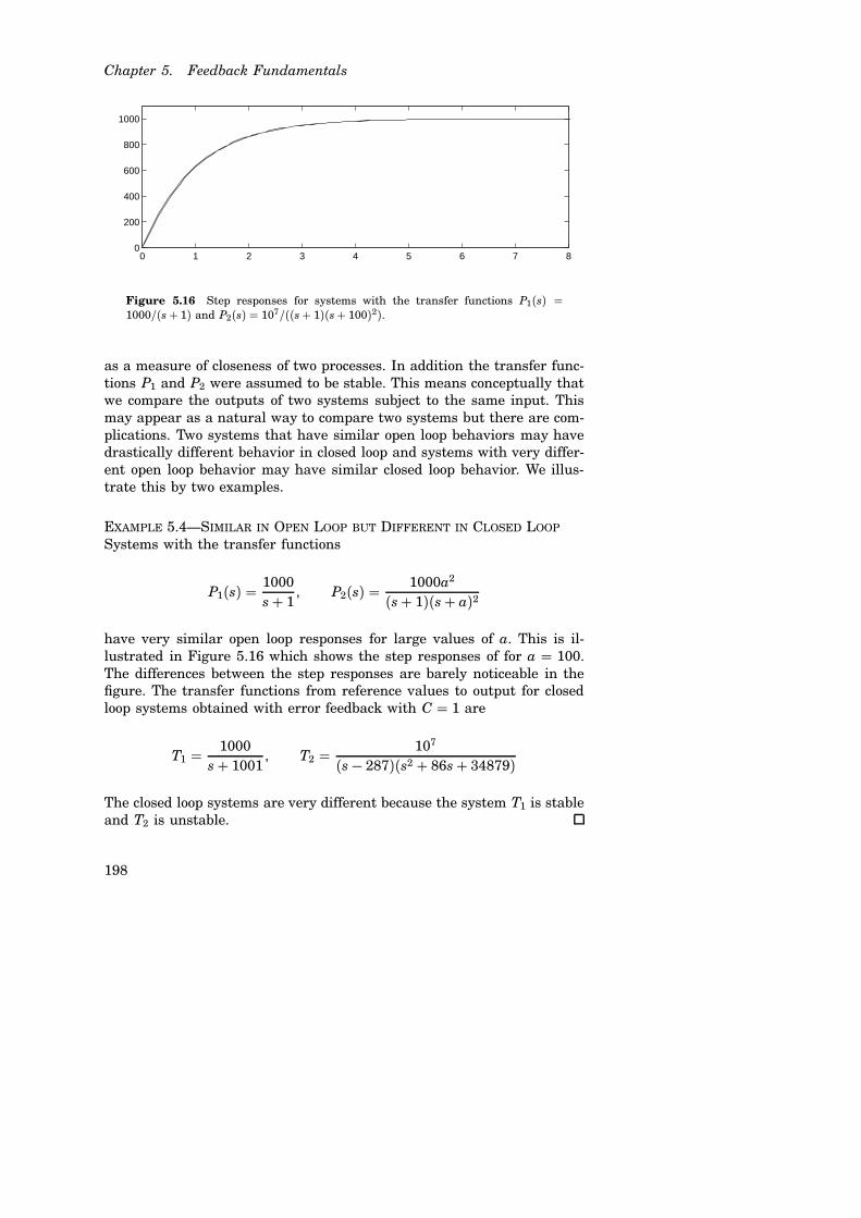
Figure 5.16 Step responses for systems with the transfer functions P1(s) =1000/(s+ 1) and P2(s) = 107/((s+ 1)(s+ 100)2).

as a measure of closeness of two processes. In addition the transfer func-tions P1 and P2 were assumed to be stable. This means conceptually thatwe compare the outputs of two systems subject to the same input. Thismay appear as a natural way to compare two systems but there are com-plications. Two systems that have similar open loop behaviors may havedrastically different behavior in closed loop and systems with very differ-ent open loop behavior may have similar closed loop behavior. We illus-trate this by two examples.

EXAMPLE 5.4—SIMILAR IN OPEN LOOP BUT DIFFERENT IN CLOSED LOOP

Systems with the transfer functions

P1(s) = 1000s+ 1

, P2(s) = 1000a2

(s+ 1)(s+ a)2

have very similar open loop responses for large values of a. This is il-lustrated in Figure 5.16 which shows the step responses of for a = 100.The differences between the step responses are barely noticeable in thefigure. The transfer functions from reference values to output for closedloop systems obtained with error feedback with C = 1 are

T1 = 1000s+ 1001

, T2 = 107

(s− 287)(s2 + 86s+ 34879)

The closed loop systems are very different because the system T1 is stableand T2 is unstable.

198


EXAMPLE 5.5—DIFFERENT IN OPEN LOOP BUT SIMILAR IN CLOSED LOOP

Systems with the transfer functions

P1(s) = 1000s+ 1

, P2(s) = 1000s− 1

have very different open loop properties because one system is unstableand the other is stable. The transfer functions from reference values tooutput for closed loop systems obtained with error feedback with C = 1are

T1(s) = 1000s+ 1001

T2(s) = 1000s+ 999

which are very close.

These examples show clearly that to compare two systems by investigatingtheir open loop properties may be strongly misleading from the pointof view of feedback control. Inspired by the examples we will insteadcompare the properties of the closed loop systems obtained when twoprocesses P1 and P2 are controlled by the same controller C. To do thisit will be assumed that the closed loop systems obtained are stable. Thedifference between the closed loop transfer functions is

δ (P1, P2) =∣∣∣ P1C1+ P1C

− P2C1+ P2C

∣∣∣ = ∣∣∣ (P1 − P2)C(1+ P1C)(1+ P2C)

∣∣∣ (5.16)

This is a natural way to express the closeness of the systems P1 and P2,when they are controlled by C. It can be verified that δ is a proper normin the mathematical sense. There is one difficulty from a practical pointof view because the norm depends on the feedback C. The norm has someinteresting properties.

Assume that the controller C has high gain at low frequencies. Forlow frequencies we have

δ (P1, P2) � P1 − P2

P1P2C

If C is large it means that δ can be small even if the difference P1− P2 islarge. For frequencies where the maximum sensitivity is large we have

δ (P1, P2) � Ms1Ms2hC(P1 − P2)h

For frequencies where P1 and P2 have small gains, typically for highfrequencies, we have

δ (P1, P2) � hC(P1 − P2)h

199


This equation shows clearly the disadvantage of having controllers withlarge gain at high frequencies. The sensitivity to modeling error for highfrequencies can thus be reduced substantially by a controller whose gaingoes to zero rapidly for high frequencies. This has been known empiricallyfor a long time and it is called high frequency roll off.

5.7 The Sensitivity Functions

We have seen that the sensitivity function S and the complementary sen-sitivity function T tell much about the feedback loop. We have also seenfrom Equations (5.6) and (5.13) that it is advantageous to have a smallvalue of the sensitivity function and it follows from (5.10) that a smallvalue of the complementary sensitivity allows large process uncertainty.Since

S(s) = 11+ P(s)C(s) and T(s) = P(s)C(s)

1+ P(s)C(s)it follows that

S(s) + T(s) = 1 (5.17)This means that S and T cannot be made small simultaneously. The looptransfer function L is typically large for small values of s and it goes tozero as s goes to infinity. This means that S is typically small for small sand close to 1 for large. The complementary sensitivity function is closeto 1 for small s and it goes to 0 as s goes to infinity.

A basic problem is to investigate if S can be made small over a largefrequency range. We will start by investigating an example.

EXAMPLE 5.6—SYSTEM THAT ADMITS SMALL SENSITIVITIES

Consider a closed loop system consisting of a first order process and aproportional controller. Let the loop transfer function

L(s) = P(s)C(s) = ks+ 1

where parameter k is the controller gain. The sensitivity function is

S(s) = s+ 1s+ 1+ k

and we have

hS(iω )h =√

1+ω 2

1+ 2k+ k2 +ω 2

200

5.7 The Sensitivity Functions

This implies that hS(iω )h < 1 for all finite frequencies and that the sensi-tivity can be made arbitrary small for any finite frequency by making ksufficiently large.

The system in Example 5.6 is unfortunately an exception. The key featureof the system is that the Nyquist curve of the process lies in the fourthquadrant. Systems whose Nyquist curves are in the first and fourth quad-rant are called positive real. For such systems the Nyquist curve neverenters the region shown in Figure 5.11 where the sensitivity is greaterthan one.

For typical control systems there are unfortunately severe constraintson the sensitivity function. Bode has shown that if the loop transfer haspoles pk in the right half plane and if it goes to zero faster than 1/s forlarge s the sensitivity function satisfies the following integral∫ ∞

0log hS(iω )hdω =

∫ ∞

0log

1h1+ L(iω )hdω = π

∑Re pk (5.18)

This equation shows that if the sensitivity function is made smaller forsome frequencies it must increase at other frequencies. This means thatif disturbance attenuation is improved in one frequency range it will beworse in other. This has been been called the water bed effect.

Equation (5.18) implies that there are fundamental limitations to whatcan be achieved by control and that control design can be viewed as aredistribution of disturbance attenuation over different frequencies.

For a loop transfer function without poles in the right half plane (5.18)reduces to ∫ ∞

0log hS(iω )hdω = 0

This formula can be given a nice geometric interpretation as shown inFigure 5.17 which shows log hS(iω )h as a function of ω . The area over thehorizontal axis must be equal to the area under the axis.

Derivation of Bode’s Formula*

This is a technical section which requires some knowledge of the theoryof complex variables, in particular contour integration. Assume that theloop transfer function has distinct poles at s = pk in the right half planeand that L(s) goes to zero faster than 1/s for large values of s. Considerthe integral of the logarithm of the sensitivity function S(s) = 1/(1 +L(s)) over the contour shown in Figure 5.18. The contour encloses theright half plane except the points s = pk where the loop transfer functionL(s) = P(s)C(s) has poles and the sensitivity function S(s) has zeros. Thedirection of the contour is counter clockwise.

201


0 0.5 1 1.5 2 2.5 3−3

−2

−1

0

1

ω

loghS(iω)h

Figure 5.17 Geometric interpretation of Bode’s integral formula (5.18).

pk

Figure 5.18 Contour used to prove Bode’s theorem.

∫Γ

log(S(s))ds =∫ −iω

iωlog(S(s))ds+

∫R

log(S(s))ds+∑

k

∫γ

log(S(s))ds

= I1 + I2 + I3 = 0

where R is a large semi circle on the right and γ k is the contour startingon the imaginary axis at s = Im pk and a small circle enclosing the polepk. The integral is zero because the function log S(s) is regular inside thecontour. We have

I1 = −i∫ iR

−iRlog(S(iω ))dω = −2i

∫ iR

0log(hS(iω )h)dω

because the real part of log S(iω ) is an even function and the imaginary

202

5.8 Reference Signals

part is an odd function. Furthermore we have

I2 =∫

Rlog(S(s))ds =

∫R

log(1+ L(s))ds �∫

RL(s)ds

Since L(s) goes to zero faster than 1/s for large s the integral goes tozero when the radius of the circle goes to infinity. Next we consider theintegral I3, for this purpose we split the contour into three parts X+, γand X− as indicated in Figure 5.18. We have∫

γlog(S(s))ds =

∫X+

log(S(s))ds+∫

γlog(S(s))ds+

∫X−

log(S(s))ds

The contour γ is a small circle with radius r around the pole pk. Themagnitude of the integrand is of the order log r and the length of thepath is 2π r. The integral thus goes to zero as the radius r goes to zero.Furthermore we have∫

X+log(S(s))ds+

∫X−

log(S(s))ds

=∫

X+

(log(S(s)) − log(S(s− 2π i))ds = 2π pk

Letting the small circles go to zero and the large circle go to infinity andadding the contributions from all right half plane poles pk gives

I1 + I2 + I3 = −2i∫ iR

0log(hS(iω )h)dω +

∑k

2π pk = 0.

which is Bode’s formula (5.18).


The response of output y and control u to reference r for the systems inFigure 5.1 having two degrees of freedom is given by the transfer functions

Gyr = PCF1+ PC

= FT

Gur = CF1+ PC

First we can observe that if F = 1 then the response to reference signalsis given by T . In many cases the transfer function T gives a satisfactory

203


response but in some cases it may be desirable to modify the response. Ifthe feedback controller C has been chosen to deal with disturbances andprocess uncertainty it is straight forward to find a feedforward transferfunction that gives the desired response. If the desired response fromreference r to output y is characterized by the transfer function M thetransfer function F is simply given by

F = MT= (1+ PC)M

PC(5.19)

The transfer function F has to be stable and it therefore follows that allright half plane zeros of C and P must be zeros of M . Non-minimum phaseproperties of the process and the controller therefore impose restrictionson the response to reference signals. The transfer function given by (5.19)can also be complicated so it may be useful to approximate the transferfunction.

Tracking of Slowly Varying Reference Signals

In applications such as motion control and robotics it may be highly de-sirable to have very high precision in following slowly varying referencesignals. To investigate this problem we will consider a system with errorfeedback. Neglecting disturbances it follows that

E(s) = S(s)R(s)

To investigate the effects of slowly varying reference signals we make aTaylor series expansion of the sensitivity function

S(s) = e0 + e1s+ e2s2 + . . . .

The coefficients ek are called error coefficients. The output generated byslowly varying inputs is thus given by

y(t) = r(t) − e0r(t) − e1dr(t)

dt− e2

d2r(t)dt2 + . . . (5.20)

Notice that the sensitivity function is given by

S(s) = 11+ P(s)C(s)

The coefficient e0 is thus zero if P(s)C(s) � 1/s for small s, i.e. if theprocess or the controller has integral action.

204


EXAMPLE 5.7—TRACKING A RAMP SIGNALS

Consider for example a ramp input

r(t) = v0t.

It follows from (5.20) that the output is given by

y(t) = v0t− e0v0t− e1v0.

The error grows linearly if e0 �= 0. If e0 = 0 there is a constant error whichis equal to e1v0 in the steady state.

The example shows that a system where the loop transfer function hasan integrator there will be a constant steady state error when trackinga ramp signal. The error can be eliminated by using feedforward as isillustrated in the next example.

EXAMPLE 5.8—REDUCING TRACKING ERROR BY FEEDFORWARD

Consider the problem in Example 5.7. Assume that e0 = 0. Introducingthe feedforward transfer function

F = 1+ f1s (5.21)

we find that the transfer function from reference to output becomes

Gyr(s) = F(s)T(s) = F(s)(1− S(s))= (1+ f1s)(1− e0 − e1s− e2s2 − . . .)= 1− e0 + ( f1(1− e0) − e1)s+ (e2 − f1e2)s2 + . . .

If the controller has integral action it follows that e0 = 0. It then followsthat the tracking error is zero if f1 = e1. The compensator (5.21) impliesthat the feedforward compensator predicts the output. Notice that twocoefficients have to be matched.

The error in tracking ramps can also be eliminated by introducing anadditional integrator in the controller as is illustrated in the next example.

EXAMPLE 5.9—REDUCING TRACKING ERROR BY FEEDBACK

Choosing F = 1 and a controller which gives a loop transfer function withtwo integrators we have

L(s) � ks2

for small s. This implies that e0 = e1 = 0 and e2 = 1/k and it follows from(5.20) that there will be no steady state tracking error. There is, however,

205


0 1 2 3 4 5 6 7 8 9 100

0.2

0.4

0.6

0.8

1

1.2

1.4

0 1 2 3 4 5 6 7 8 9 100

2

4

6

8

10

Ste

pre

spon

seR

amp

resp

onse

Time

Time

Figure 5.19 Step (above) and ramp (below) responses for a system with errorfeedback having e0 = e1 = 0.

one disadvantage with a loop transfer function having two integratorsbecause the response to step signals will have a substantial overshoot.The error in the step response is given by

E(s) = S(s)1s

The integral of the error is

E(s)s

= S(s) 1s2

Using the final value theorem we find that

limt→∞

∫ t

0e(τ )dτ = lim

s→0

sS(s)s2 = 0

Since the integral of the error for a step in the reference is zero it meansthat the error must have an overshoot. This is illustrated in Figure 5.19.This is avoided if feedforward is used.

The figure indicates that an attempt to obtain a controller that givesgood responses to step and ramp inputs is a difficult compromise if the

206

5.9 Fundamental Limitations

controller is linear and time invariant. In this case it is possible to resolvethe compromise by using adaptive controllers that adapt their behaviorto the properties of the input signal.

Constraints on the sensitivities will, in general, give restrictions on theclosed loop poles that can be chosen. This implies that when controllersare designed using pole placements it is necessary to check afterwardsthat the sensitivities have reasonable values. This does in fact apply to alldesign methods that do not introduce explicit constraints on the sensitivityfunctions.


In any field it is important to be aware of fundamental limitations. In thissection we will discuss these for the basic feedback loop. We will discusshow quickly a system can respond to changes in the reference signal.Some of the factors that limit the performance are

• Measurement noise

• Actuator saturation

• Process dynamics

Measurement Noise and Saturations

It seems intuitively reasonable that fast response requires a controllerwith high gain. When the controller has high gain measurement noise isalso amplified and fed into the system. This will result in variations inthe control signal and in the process variable. It is essential that the fluc-tuations in the control signal are not so large that they cause the actuatorto saturate. Since measurement noise typically has high frequencies thehigh frequency gain Mc of the controller is thus an important quantity.Measurement noise and actuator saturation thus gives a bound on thehigh frequency gain of the controller and therefore also on the responsespeed.

There are many sources of measurement noise, it can caused by thephysics of the sensor, in can be electronic. In computer controlled systemsit is also caused by the resolution of the analog to digital converter. Con-sider for example a computer controlled system with 12 bit AD and DAconverters. Since 12 bits correspond to 4096 it follows that if the highfrequency gain of the controller is Mc = 4096 one bit conversion error willmake the control signal change over the full range. To have a reasonablesystem we may require that the fluctuations in the control signal dueto measurement noise cannot be larger than 5% of the signal span. This

207


means that the high frequency gain of the controller must be restrictedto 200.

Dynamics Limitations

The limitations caused by noise and saturations seem quite obvious. Itturns out that there may also be severe limitations due to the dynamicalproperties of the system. This means that there are systems that areinherently difficult or even impossible to control. It is very importantfor designers of any system to be aware of this. Since systems are oftendesigned from static considerations the difficulties do not show up becausethey are dynamic in nature. A brief summary of dynamic elements thatcause difficulties are summarized briefly.

It seems intuitively clear that time delay cause limitations in the re-sponse speed. A system clearly cannot respond in times that are shorterthan the time delay. It follows from

e−sTd � 1− sTd/21+ sTd/2 =

s− 2/Td

s+ 2/Td= s− z

s+ z(5.22)

that a zero in the right half plane z can be approximated with a timedelay Td = 2/z and we may thus expect that zeros in the right half planealso cause limitations. Notice that a small zero corresponds to a long timedelay.

Intuitively it also seems reasonable that instabilities will cause lim-itations. We can expect that a fast controller is required to control anunstable system.

Summarizing we can thus expect that time delays and poles and zerosin the right half plane give limitations. To give some quantitative resultswe will characterize the closed loop system by the gain crossover frequencyω nc. This is the smallest frequency where the loop transfer function hasunit magnitude, i.e. hL(iω nc)h. This parameter is approximately inverselyproportional to the response time of a system. The dynamic elements thatcause limitations are time delays and poles and zeros in the right halfplane. The key observations are:

• A right half plane zero z limits the response speed. A simple rule ofthumb is

ω nc < 0.5z (5.23)Slow RHP zeros are thus particularly bad.

• A time delay Td limits the response speed. A simple rule of thumbis

ω ncTd < 0.4 (5.24)

208


• A right half plane pole p requires high gain crossover frequency. Asimple rule of thumb is

ω nc > 2p (5.25)Fast unstable poles require a high crossover frequency.

• Systems with a right half plane pole p and a right half plane zero zcannot be controlled unless the pole and the zero are well separated.A simple rule of thumb is

p > 6z (5.26)

• A system with a a right half plane pole and a time delay Td cannotbe controlled unless the product pTd is sufficiently small. A simplerule of thumb is

pTd < 0.16 (5.27)

We illustrate this with a few examples.

EXAMPLE 5.10—BALANCING AN INVERTED PENDULUM

Consider the situation when we attempt to balance a pole manually. Aninverted pendulum is an example of an unstable system. With manualbalancing there is a neural delay which is about Td = 0.04 s. The transferfunction from horizontal position of the pivot to the angle is

G(s) = s2

s2 − nQ

where n = 9.8 m/s2is the acceleration of gravity and Q is the length of thependulum. The system has a pole p =

√n/Q. The inequality (5.27) gives

0.04√n/Q = 0.16

Hence, Q = 0.6 m. Investigate the shortest pole you can balance.

EXAMPLE 5.11—BICYCLE WITH REAR WHEEL STEERING

The dynamics of a bicycle was derived in Section 4.3. To obtain the modelfor a bicycle with rear wheel steering we can simply change the sign of thevelocity. It then follows from (4.9) that the transfer function from steeringangle β to tilt angle θ is

P(s) = mV0Qb

Js2 −mnl−as+ V0

209


Notice that the transfer function depends strongly on the forward velocityof the bicycle. The system thus has a right half plane pole at p =

√mnQ/J

and a right half plane zero at z = V0/a, and it can be suspected that thesystem is difficult to control. The location of the pole does not depend onvelocity but the the position of the zero changes significantly with velocity.At low velocities the zero is at the origin. For V0 = a

√mnQ/J the pole and

the zero are at the same location and for higher velocities the zero is tothe right of the pole. To draw some quantitative conclusions we introducethe numerical values m = 70 kg, Q = 1.2 m, a = 0.7, J = 120 kgm2 andV = 5 m/s, give z = V/a = 7.14 rad/s and p = ω 0 = 2.6 rad/s we findthat p = 2.6. With V0 = 5 m/s we get z = 7.1, and p/z = 2.7. To have asituation where the system can be controlled it follows from (5.26) thatto have z/p = 6 the velocity must be increased to 11 m/s. We can thusconclude that if the speed of the bicycle can be increased to about 10 m/sso rapidly that we do not loose balance it can indeed be ridden.

The bicycle example illustrates clearly that it is useful to assess the funda-mental dynamical limitations of a system at an early stage in the design.If this had been done the it could quickly have been concluded that thestudy of rear wheel steered motor bikes in 4.3 was not necessary.

Remedies

Having understood factors that cause fundamental limitations it is inter-esting to know how they should be overcome. Here are a few suggestions.

Problems with sensor noise are best approached by finding the rootsof the noise and trying to eliminate them. Increasing the resolution ofa converter is one example. Actuation problems can be dealt with in asimilar manner. Limitations caused by rate saturation can be reduced byreplacing the actuator.

Problems that are caused by time delays and RHP zeros can be ap-proached by moving sensors to different places. It can also be beneficial toadd sensors. Recall that the zeros depend on how inputs and outputs arecoupled to the states of a system. A system where all states are measuredhas no zeros.

Poles are inherent properties of a system, they can only be modifiedby redesign of the system.

Redesign of the process is the final remedy. Since static analysis cannever reveal the fundamental limitations it is very important to make anassessment of the dynamics of a system at an early stage of the design.This is one of the main reasons why all system designers should have abasic knowledge of control.

210

5.10 Electronic Amplifiers

V1

R2R1+R2 Σ −A

R1R1+R2

V V2

Figure 5.20 Block diagram of the feedback amplifier in Figure 2.9. Compare withFigure 2.10


There are many variations on the prototype problem discussed in Sec-tion 5.2. To illustrate this we will discuss electronic amplifiers. Examplesof such amplifiers have been given several times earlier, see Section 1.8and Example 2.3.

The key issues in amplifier design are gain, noise and process varia-tions. The purpose of an electronic amplifier is to provide a high gain anda highly linear input output characteristics. The main disturbance is elec-trical noise which typically has high frequencies. There are variations inthe components that create nonlinearities and slow drift that are causedby temperature variations. A nice property of feedback amplifiers thatdiffer from many other processes is that many extra signals are availableinternally.

The difficulty of finding a natural block diagram representation of asimple feedback amplifier was discussed in Example 2.3. Some alternativeblock diagram representations were given in Figure 2.10. In particularwe noted the difficulty that there was not a one to one correspondencebetween the components and the blocks. We will start by showing yetanother representation. In this diagram we have kept the negative gainof the feedback loop in the forward path and the standard −1 block hasbeen replaced by a feedback. It is customary to use diagrams of this typewhen dealing with feedback amplifiers. The generic version of the diagramis shown in Figure 5.21. The block A represents the open loop amplifier,block F the feedback and block H the feedforward. The blocks F and Hare represented by passive components.

211


R2R1+R2

−A

R1R1+R2

ΣΣV1 V

n

V2

Figure 5.21 Generic block diagram of a feedback amplifier.

For the circuit in Figure 5.20 we have

F = R1

R1 + R2

H = R2

R1 + R2

notice that both F and H are less than one.

The Gain Bandwidth Product

The input-output relation for the system in Figure 5.21 is given by

LV2

LV1= −G

where

G = AH1+ AF

(5.28)The transfer function of an operational amplifier can be approximated by

A(s) = bs+ a

The amplifier has gain b/a and bandwidth a. The gain bandwidth productis b. Typical numbers for a simple operational amplifier that is often usedto implement control systems, LM 741, are a = 50 Hz, b = 1 MHz. Otheramplifiers may have gain bandwidth products that are several orders ofmagnitude larger.

Furthermore we have

F = R1

R1 + R2, H = R2

R1 + R2

212


10−2

10−1

100

101

102

103

104

105

106

100

102

104

106

ω

Gai

n

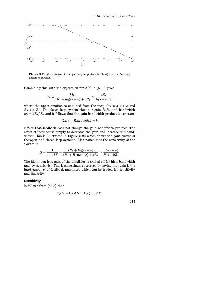
Figure 5.22 Gain curves of the open loop amplifier (full lines) and the feedbackamplifier (dashed)

Combining this with the expression for A(s) in (5.28) gives

G = bR2

(R1 + R2)(s+ a) + bR1� bR2

R2s+ bR1

where the approximation is obtained from the inequalities b >> a andR2 >> R1. The closed loop system thus has gain R2 R1 and bandwidthω 0 = bR1/R2 and it follows that the gain bandwidth product is constant

Gain� Bandwidth = b

Notice that feedback does not change the gain bandwidth product. Theeffect of feedback is simply to decrease the gain and increase the band-width. This is illustrated in Figure 5.22 which shows the gain curves ofthe open and closed loop systems. Also notice that the sensitivity of thesystem is

S = 11+ AF

= (R1 + R2)(s+ a)(R1 + R2)(s+ a) + bR1

� R2(s+ a)R2s+ bR1

The high open loop gain of the amplifier is traded off for high bandwidthand low sensitivity. This is some times expressed by saying that gain is thehard currency of feedback amplifiers which can be traded for sensitivityand linearity.

Sensitivity

It follows from (5.28) that

log G = log AH − log (1+ AF)

213


Differentiating this expression we find that

d log Gd log A

= 11+ AF

d log Gd log F

= − AF1+ AF

d log Gd log H

= 1

The loop transfer function is normally large which implies that it is onlythe sensitivity with respect the amplifier that is small. This is, how-ever, the important active part where there are significant variations.The transfer functions F and H typically represent passive componentsthat are much more stable than the amplifiers.

Signal to Noise Ratio

The ratio between signal and noise is an important parameter for anamplifier. Noise is represented by the signals n1 and n2 in Figure 5.21.Noise entering at the amplifier input is more critical than noise at theamplifier output. For an open loop system the output voltage is given by

Vol = N2 − A(N1 + HV1)

For a system with feedback the output voltage is instead given by

Vcl = 11+ AF

(N2 − A(N1 + HV1)

) = 11+ AF

Vol

The signals will be smaller for a system with feedback but the signal tonoise ratio does not change.

5.11 Summary

Having got insight into some fundamental properties of the feedback loopwe are in a position to discuss how to formulate specifications on a controlsystem. It was mentioned in Section 5.2 that requirements on a controlsystem should include stability of the closed loop system, robustness tomodel uncertainty, attenuation of measurement noise, injection of mea-surement noise ability to follow reference signals. From the results givenin this section we also know that these properties are captured by six

214

5.11 Summary

transfer functions called the Gang of Six. The specifications can thus beexpressed in terms of these transfer functions.

Stability and robustness to process uncertainties can be expressed bythe sensitivity function and the complementary sensitivity function

S = 11+ PC

, T = PC1+ PC

.

Load disturbance attenuation is described by the transfer function fromload disturbances to process output

Gyd = P1+ PC

= PS.

The effect of measurement noise is be captured by the transfer function

−Gun = C1+ PC

= CS,

which describes how measurement noise influences the control signal. Theresponse to set point changes is described by the transfer functions

Gyr = FPC1+ PC

= FT , Gur = FC1+ PC

= FCS

Compare with (5.1). A significant advantage with controller structurewith two degrees of freedom is that the problem of set point response canbe decoupled from the response to load disturbances and measurementnoise. The design procedure can then be divided into two independentsteps.

• First design the feedback controller C that reduces the effects ofload disturbances and the sensitivity to process variations withoutintroducing too much measurement noise into the system

• Then design the feedforward F to give the desired response to setpoints.

215

feedback fundamentals - caltech computingmurray/courses/cds101/fa02/caltech/a... · ration of the...

Documents