FEDERAL RURAL UNIVERSITY OF PERNAMBUCO

DEPARTMENT OF ANIMAL SCIENCE

GRADUATE PROGRAM IN ANIMAL SCIENCE

STABLE ISOTOPES IN THE RUMINANT DIETARY IDENTIFICATION

JOSE DIOGENES PEREIRA NETO

RECIFE-PE

JULY 2017

JOSE DIOGENES PEREIRA NETO

STABLE ISOTOPES IN THE RUMINANT DIETARY IDENTIFICATION

Thesis presented to the graduate

program in animal science of

Federal Rural University of

Pernambuco, required to obtain,

partially, the Master degree of

sciences.

Committee:

Prof. PhD. Jose Carlos Batista Dubeux Junior - Chair

Prof. PhD. Mercia Virginia Ferreira dos Santos – Co-chair

Prof. PhD. Francisco Fernando Ramos de Carvalho – Co-chair

RECIFE-PE

JULY 2017

JOSE DIOGENES PEREIRA NETO

Stable isotopes in the ruminant dietary identification

Thesis defended and approved by the examination committee in 28 July 2017.

Examination Committee:

________________________________________

Prof. PhD. Jose Carlos Batista Dubeux Junior

Federal Rural University of Pernambuco

Animal Science Department

Chair

________________________________________

Prof. PhD. Everardo Valadares de Sá Barretto Sampaio

Federal University of Pernambuco

Nuclear Energy Department

________________________________________

Prof. PhD. Dulciene Karla de Andrade Silva

Federal Rural University of Pernambuco

UAG/Animal Science Department

RECIFE-PE

JULY 2017

ACKNOWLEDGMENTS

My GOD, my LORD. You are my strength, happiness, and reason to live.

The Federal Rural University of Pernambuco, CNPq, and Graduate program in animal science,

for this opportunity.

My parents, Carlos and Suely

My Family, wife Bruna, and my son Lucas, which are a piece of me. I love you.

I would like to thank my Mother in law, for prays.

I would like to thank my advisor Professor Jose Carlos Batista Dubeux Junior (Jose Dubeux).

Thank you for everting, you made it happen.

My co-Advisor, Professor Mercia V. F. dos Santos, for all the support, and my co-advisor

Professor, since my undergraduate, Francisco F. R. de Carvalho, which was always ready to

help me.

I would like to thank Professor Nicolas DiLorenzo and Martin Ruiz-Moreno, thanks for your

support in this thesis, for your knowledge, and for the sample analyses. I extend this gratitude

to all the professors and staff, from UFRPE and UF-IFAS NFREC.

I would like to thank all my friends, that helped me in the field trial, thanks a lot. All of you

from DZ-UFRPE are amazing. Thanks also to Pedro and Jonas (Lebre) for the support with the

animals.

I would like to thank all my friends from the graduate program, such as Michelle Siqueira,

Carol Vasco, Elayne Soares, Nubia Meirely, Joao Vitor, Luiz Wilker, Karen Abreu, Marina

Almeida, Tony Carvalho, Janaina Lima, Wandenberg Rocha, Heraclito Lima, Fernanda

Dantas, Rayanne Souza, Thamires Quiniro, Karina Miranda, and all the people, thanks for the

friendship.

I would like to thank all my friends from Marianna - FL, NFREC, my second house. Erick

Rodrigo (a brother), David Jaramillo (a little brother), Pedro Levy (a Big Brother), Gleise

Medeiros (a sister), Nicky Oosthuizen (my little fish), Luana Mayara, Liza Garcia, Jose

Rolando, Marco Goyzueta, Hiran Marcelo (big master) and Joyce Patu. Thanks for make my

journey pleasant.

Thanks…

Have not I commanded you? Be strong and of a good courage; be not afraid, neither be you

dismayed: for the LORD your God is with you wherever you go.

Joshua 1:9

SUMMARY

Page

List of Tables ……………………………………………………………………... iiiv

List of Figures ………………………………………………………………..…... ix

Chapter 1…………………………………………………………………………. 10

Introduction ……...………………………………………………………………. 11

Literature Review …………..…………………………………………………….. 13

1. Grassland ………………………………………………………………….. 13

2. Mixed grass-legume pastures ……………………………………………… 14

2.1 Legume Pasture………………………………………………………… 14

3. Intake ………………………………………………………………………. 16

3.1 Forage Intake……….………………………………………………….. 16

3.2 Methods to estimate forage intake ……………………………………… 17

3.2.1 Direct methods …………….…………………………………… 17

3.2.2 Indirect methods………………………………………………... 18

3.2.3 Fecal output estimate ……….…………………………………. 18

3.2.4 Forage digestibility ……………………………………………. 20

4. Stable Isotopes……………………………………………………................ 21

4.1 Stable Isotope Definition ……………………………………………….. 21

4.2 Isotope Notation ……………………………………………………….. 21

4.3 Isotope measurement ……………………………………….…………. 23

4.4 Isotope Samples…………………………………………..……………. 24

4.5 Isotope technique and field analysis …………………..……………….. 24

5 Carbon Stable isotopes ………………………………………………………… 25

5.1 Stable Isotope Carbon Natural Abundance …………………………… 26

5.2 C3 and C4 plants 12C/13C discrimination ………………………………. 27

6 Carbon stable isotopes and the reconstruction of animal diets……………….. 28

6.1 Carbon analysis technique for animal diet …………………………… 28

6.2 Back calculation of animal diets using stable isotopes……..………..… 29

6.3 Difference between dietary and animal tissue δ13C……………………. 30

6.3.1. Diet-animal sample discrimination…….………………………… 30

6.3.2 Fecal endogenous contamination ………………………………… 31

6.3.3 Different digestibility and δ13C value of animal dietary ………… 32

7 Discrimination of δ13C in different plant tissues ……………………………….. 32

References ………………………………………………………………………... 34

Chapter II ……………………………………………………..…………………... 40

Resumo……………….………………………………………………………..…................. 41

Abstract ……………….…………………………………………………………................. 42

Introduction ………………………………………………………………………………… 43

Material and Methods …………………………………………………………………….. 45

Results and Discussion ……………………………………………………………………. 50

Conclusion ………………….…………………………………………….......................... 63

References ……………………………….………………………………………... 64

LIST OF TABLES

Chapter II

page

Table 1. Chemical composition of Alfalfa and Tifton 85 hay at different

inclusion levels

46

Table 2. Intake (g DM head-1 d-1 and %BW), legume and grass intake (g DM

head-1 d-1), and total fecal output (g DM head-1 d-1) of sheep fed by different

levels of Alfalfa and Tifton 85 hay

57

Table 3. Total apparent digestibility (g kg-1), and Alfalfa and Tifton 85 apparent

digestibility (g kg-1) on sheep fed by different levels of alfalfa and Tifton 85 hay

53

Table 4. Dietary and fecal δ13C (‰) and discrimination (‰) based on total

sample C and iNDF treated samples

56

Table 5. Models using total sample carbon and iNDF δ13C to trace back the diet

of ruminants

60

LIST OF FIGURES

Chapter II

page

Figure 1. Proportion of C4 plant in the diet predicted by models, using total

carbon values

61

Figure 2. Proportion of C4 plant in the diet predicted by models, using iNDF

values

62

Chapter 1

Utilization of carbon stable isotopes in the ruminant dietary identification

11

1

Introduction 2

3

Animal production is based on nutrition. Pastures are the major components in many 4

livestock production systems, and in most cases, they are solely composed by grass. As an 5

alternative to reduce the costs, mitigate the impacts of inorganics fertilizers, and improve forage 6

quality, the combination of grass and legume in the pasture, has been used around the world 7

(Muir et al., 2011; Lüscher et al., 2014). In addition, legumes can, also, improve the 8

digestibility of grasses, when consumed in legume-grass mixtures (Muir et al., 2014). 9

The forage consumption is very important to animal production. There are several 10

methods to determine the forage intake, and many of them are based on total fecal output and 11

forage digestibility (Minson, 1990; Burns et al., 1994). The forage digestibility is also an 12

important factor to estimate the intake, thus the digestibility assessment has to be accurate, 13

which is not always an easy task in grazing trials. 14

When grazing occurs in grass-legume mixed pastures, digestibility determination is 15

more challenging because of animal selection. Different proportions of grass and legume affect 16

directly the digestibility. Stable isotopes have been used as a tool, for decades, to find out the 17

digestibility of mixed diets (Jones et al., 1979; Martinez del Rio et al., 2009; Wolf et al., 2009). 18

The carbon stable isotope ratio (13C:12C) can be used to identify plants that have different 19

photosynthetic pathway, such as C3, C4, and CAM, and can be used to evaluate their presence 20

in the diet, by analyses of the feces (Martinez del Rio et al., 2009). 21

Legumes and tropical grasses have different δ13C. The grass has a δ13C value range of 22

-9‰ to -17‰, and the legume from -20‰ to -32‰ (Ballentine et al., 1998). These values can 23

be used to identify the proportions of legume and grass in the feces. Therefore, it is possible to 24

estimate the proportion of C3 and C4 species consumed by livestock grazing grass-legume 25

12

pastures. Fecal δ13C values are often more depleted than the dietary values because of 26

discrimination against the heavy isotope. The use of feces and diet to find the proportions of 27

legume and grass need to be validated because it is species specific. 28

The objective of this research is to validate the use of the carbon stable isotope ratio 29

(δ13C) to determine the proportions of C3 and C4 species in the diet based on fecal δ13C 30

determination, evaluating the prediction models using indigestible neutral detergent fiber 31

(iNDF) procedure and untreated samples. 32

13

Literature Review 33

34

35

1. Grassland 36

Grassland is the land and the vegetation growing on it devoted to the production of 37

introduced or indigenous forages, including grasses, legumes and other forbs, and at times other 38

woody species (Allen et al., 2011). Grasslands are one of the largest terrestrial agroecosystems. 39

They cover approximately 40.5 percent of the terrestrial area on Earth, except the poles, 40

equating to 52.5 million km2. Grasslands provide ecosystem services (ES) such as provision of 41

forage for domestic livestock, carbon (C) sequestration, water catchment and filtration, habitat 42

for wildlife, nutrient cycling, and many others (Dubeux et al., 2014). Provisional ES have a 43

direct economic impact, benefiting many millions of farmers to produce meat, milk, wool and 44

other animal commodities (White et al., 2000). Forage obtained from grasslands provides feed 45

and nutrients to animals at lower cost than concentrate feeds, though forages can vary in 46

nutritive value due to differences in species, environment, and timing of harvest (Givens et al., 47

2000). In many cases, it is more economically feasible to let animals graze rather than to 48

provide supplementation, since profits may be reduced by providing supplements (Redmon & 49

Hendrickson, 2007). 50

Grazing can potentially be a sustainable activity that does not burden the environment. 51

Specific subsystems such as sowed pasture and natural pasture need special attention to avoid 52

losses in economic and environmental contributions due to negative management (Rótolo et 53

al., 2007). Intensification of the grazing system is generally linked to nutrient inputs via 54

commercial fertilizers and supplement feed to animals. Excess of nutrients deposited in 55

intensive grazing systems by fertilizer and animal wastes can cause environmental disturbance. 56

Areas where animals congregate such as feedlots and dairy farms are even more problematic 57

14

regarding nutrient losses to the environment (Vendramini et al., 2007). In conventional grass-58

only pastures, the grass production depends on the use of synthetic nitrogen (N) fertilizer, in 59

order to provide a high-quality forage, but this supply has a cost, that influences cattle 60

production. Incorporating legumes into grass pastures has potential to supply N, reducing 61

production costs (Butler et al., 2012). Some economic and environment factors affect pasture 62

management. Rational use of grasslands and grass-legume mixtures are an important option to 63

improve management (Muir et al., 2011). 64

2. Mixed grass-legume pastures 65

2.1 Legume pasture 66

Improvement of soil N and the potential increase on sward production with reduced N 67

fertilizer application are advantages of using legumes in grazing systems, considering that 68

legumes are recognized as a source of biologically fixed N (Ledgard & Steele, 1992). These 69

facts are essential to understand the role of legumes in the production system and their 70

contribution to ruminant livestock production. Due to their nutritive value and ability to fix 71

atmospheric N2 via association with soil microorganisms, legumes have been used in many 72

grassland systems around the world (Rochon et al., 2004). Ledgard (2001) reported that many 73

studies indicate inputs of 200 to 400 kg N ha-1 yr-1 by forage legumes to the soil-plant-animal. 74

Field studies, however, demonstrate limitations that reduce this potential fixation to 20 to 200 75

kg N ha-1 yr-1. Rotz et al. (2005) obtained mean annual N2-fixation rates of white clover ranging 76

from 0 to 166 kg N ha-1. Cadisch et al. (1994) considered sufficient to sustain the productivity 77

of the mixed pasture system 60 to 117 kg N ha-1 year-1, and reported that the inclusion of 78

persistent legumes can improve the sustainability of pasture production. 79

Industrial fertilizers contribute indirectly to enhance soil C via increase in primary 80

productivity; however, during the manufacturing process of fertilizers, there is a release of CO2 81

15

to atmosphere (Schlesinger, 2009). Pastures with 25% of nodulating legumes in their botanical 82

composition fixing 60 kg N ha-1 year-1 were equivalent to pastures receiving 100 kg N ha-1 83

year-1 of inorganic fertilization (Lira et al. 2006). Mixed grass-legume systems, can contribute 84

with 10-75 kg N ha-1 year-1 to grass, via legume (Nyfeler et al., 2011). The establishment of N-85

fixing legumes provides benefits, such as improvement of soil organic matter (Deyn et al., 86

2011). Therefore, including forage legumes and reducing the use of industrial N fertilizer will 87

mitigate the carbon footprint of livestock production systems, contributing to reduce the 88

greenhouse effect. 89

Legumes contribute to enhance soil fertility and increase pasture production. 90

Furthermore, they can also be an excellent source of N for animal nutrition, depending on their 91

nutritive value. Sleugh et al. (2000) evaluated seasonal yield distribution and forage quality of 92

grass-legume mixtures. They observed that grass-legume mixtures can improve the nutritive 93

value and seasonal distribution of forage yield, reducing the need for livestock 94

supplementation. Cantarutti et al. (2002) evaluated the effect of a legume (Desmodium 95

ovalifolium) in swards of Brachiaria humidicola. The presence of legume significantly 96

increased herbage N concentration and N recycled via litter deposition, ranging from 42 to 155 97

kg N ha-1 year -1 for 4 and 2 head ha-1, respectively. Muir et al. (2011) performed a meta-98

analysis and observed that, for warm-season grass, minimum crude protein (CP) concentration 99

was 78 ± 9 g kg-1 and for legume was 151 ± 9 g kg-1. They concluded that the most important 100

nutritional contribution from legumes to grass-legume mixture is to provide CP for ruminants. 101

In grass-legume mixtures, grazing animals can build their diet selecting different forage species 102

and varying nutrient concentration, reaching their nutritional requirement (Gregorini et al., 103

2015). 104

105

106

16

3. Intake 107

3.1 Forage intake 108

Feed intake is essential for animal nutrition, in order to ingest the necessary nutrients 109

for maintenance and performance (Van Soest, 1994). Intake is defined by Mertens (1994) as 110

the absolute amount of dry matter (DM) ingested per unit of time. Intake is often measured 111

over a period of 5 to 10 days, and it is expressed as daily quantity per unit of body weight 112

(BW). Intake and digestibility are considered the major components determining ruminant 113

production (Mertens, 2007). 114

Factors such as animal, forage, and environmental conditions can control forage intake. 115

Under grazing, however, some factors are unique, such as preference, bite size, water content 116

of forage, herbage mass, herbage accumulation, herbage allowance, and sward heterogeneity 117

(Minson, 1990; Minson and Wilson, 1994). Grazing factors can influence the intake 118

measurement, due to the possibility of animals to select parts of the plant or plant species. 119

Selection indicate preferential consumption of a feed subcomponent, such as parts of plant and 120

plants within a specific physiological state (Mertens, 1994). Through selective grazing, animals 121

are free to search for feed and select the diet, increasing its nutritional diet. In order to achieve 122

this goal, they develop their own feeding strategy (Baumont et al., 2000). 123

The measurement of DM intake (DMI) for grazing animals can be laborious and time 124

consuming. Handling the animal intake and the fecal output collection are more difficult to 125

accomplish in pastures than housed animals. As a result, these measurements, under grazing 126

conditions, are hard to obtain with accuracy (Van Soest, 1994; Gregorini et al., 2015). In mixed 127

pastures and rangelands, the problem might become worst because of the heterogeneity of the 128

vegetation (Oltjen et al., 2015). Estimating diet selection is not a simple task in complex 129

grazing situation, such as rangelands, with several forage species (Baumont et al., 2000). 130

131

17

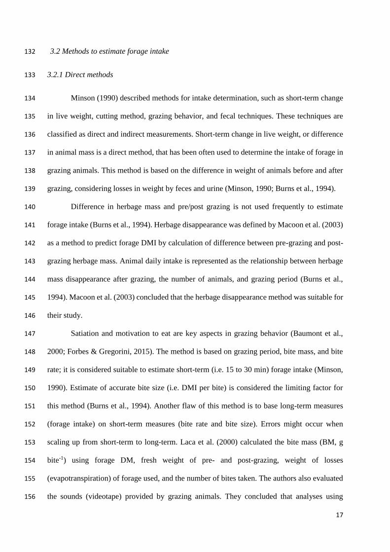
3.2 Methods to estimate forage intake 132

3.2.1 Direct methods 133

Minson (1990) described methods for intake determination, such as short-term change 134

in live weight, cutting method, grazing behavior, and fecal techniques. These techniques are 135

classified as direct and indirect measurements. Short-term change in live weight, or difference 136

in animal mass is a direct method, that has been often used to determine the intake of forage in 137

grazing animals. This method is based on the difference in weight of animals before and after 138

grazing, considering losses in weight by feces and urine (Minson, 1990; Burns et al., 1994). 139

Difference in herbage mass and pre/post grazing is not used frequently to estimate 140

forage intake (Burns et al., 1994). Herbage disappearance was defined by Macoon et al. (2003) 141

as a method to predict forage DMI by calculation of difference between pre-grazing and post-142

grazing herbage mass. Animal daily intake is represented as the relationship between herbage 143

mass disappearance after grazing, the number of animals, and grazing period (Burns et al., 144

1994). Macoon et al. (2003) concluded that the herbage disappearance method was suitable for 145

their study. 146

Satiation and motivation to eat are key aspects in grazing behavior (Baumont et al., 147

2000; Forbes & Gregorini, 2015). The method is based on grazing period, bite mass, and bite 148

rate; it is considered suitable to estimate short-term (i.e. 15 to 30 min) forage intake (Minson, 149

1990). Estimate of accurate bite size (i.e. DMI per bite) is considered the limiting factor for 150

this method (Burns et al., 1994). Another flaw of this method is to base long-term measures 151

(forage intake) on short-term measures (bite rate and bite size). Errors might occur when 152

scaling up from short-term to long-term. Laca et al. (2000) calculated the bite mass (BM, g 153

bite-1) using forage DM, fresh weight of pre- and post-grazing, weight of losses 154

(evapotranspiration) of forage used, and the number of bites taken. The authors also evaluated 155

the sounds (videotape) provided by grazing animals. They concluded that analyses using 156

18

grazing sounds can solve some problems related with measurements of grazing intake. Forbes 157

and Gregorini (2015) presented feed intake (g day-1) as a function of meal frequency (meals 158

day-1) and meal size (g meal-1). 159

3.2.2 Indirect methods 160

A variety of indirect and complex techniques has been evolved, due to difficulty of 161

measuring forage DMI in grazing animals (Burns et al., 1994; Van Soest, 1994). In past 162

decades, the technique to estimate the forage intake of grazing animals by determining total 163

fecal output was described. The method is simple, using bags to collect feces and the apparent 164

digestibility of the forage, obtained by animals in feedlot (Minson, 1990). In order to calculate 165

the DMI of grazing animals, it is necessary to know the fecal output (FO) and digestibility. The 166

equation to estimate DMI was described by Minson (1990) and Carvalho et al. (2007) as: 167

168

Intake (g DM/day)= Feces output/(1-DM forage digestibility ) 169

170

3.2.3 Fecal output estimate 171

There are two ways to obtain the fecal output, direct and indirect. The direct way 172

involves total fecal collection using collection bags placed on animals. Indirect estimate using 173

markers is less invasive. Burns et al. (1994) indicated that total fecal output can be estimated 174

by the ratio between the quantity of a marker dosed to an animal and its concentration in the 175

feces. 176

177

Markers are classified as internal or external, due to the difference of nature of the 178

compound and application, because, the external marker needs to be ingested by the animal, 179

which is an invasive method. External markers are indigestible components added in the diet 180

19

to be retrieved from the feces, or dosed in the animal. This method is indicated for animals 181

under grazing conditions. Examples of external markers used in studies include, n-alkane, 182

chromium oxide, polyethylene glycol (PEG), and LIPE® (Carvalho et al., 2007; Azevedo et 183

al., 2014; Benvenutti et al., 2014). Pulse-dose marker is a method that permit the inert marker 184

application just once, with frequent collections thereafter (Burns et al., 1994; Macoon et al. 185

2003). 186

Chromium-mordant fiber is another approach to use chromium as a marker. Hand-187

plucked forage samples are necessary to simulate the grazing and represent the forage used as 188

source of fiber to bind with the chromium (Macoon et al., 2003). The n-alkanes are used as an 189

internal (plant) and external (dosed) marker to provide an estimate of diet composition, forage 190

intake, and fecal production (Dove and Mayes, 2005). The n-alkane marker was used by 191

Azevedo et al. (2014), and reported the importance of a rigorous methodology to collect 192

samples, especially from pasture, in order to obtain a representative plant portion, as well as 193

the fecal estimative. The daily-dose marker is a method in which markers are administered 194

twice per day; it is considered a laborious technique, and can cause stress on animals (Burns et 195

al., 1994). Daily doses are applied according to the animal weight, approximately 0.5 to 1 g for 196

sheep and 5 to 10 g for cattle (Carvalho et al., 2007). Feces collection to determine marker 197

concentration can be conducted directly from the animal, by rectum grab, during weighing, 198

milking, or any other routine procedure with the animals. Another approach to collect the feces 199

is by observing animals in the pasture and collecting fecal samples right after defecation 200

(Macoon et al., 2003). 201

202

Internal markers are compounds found in the feed that are indigestible. Fecal protein, 203

indigestible dry matter (iDM), indigestible neutral detergent fiber (iNDF), and indigestible acid 204

detergent fiber (iADF) are examples of internal markers that have been used in many studies 205

20

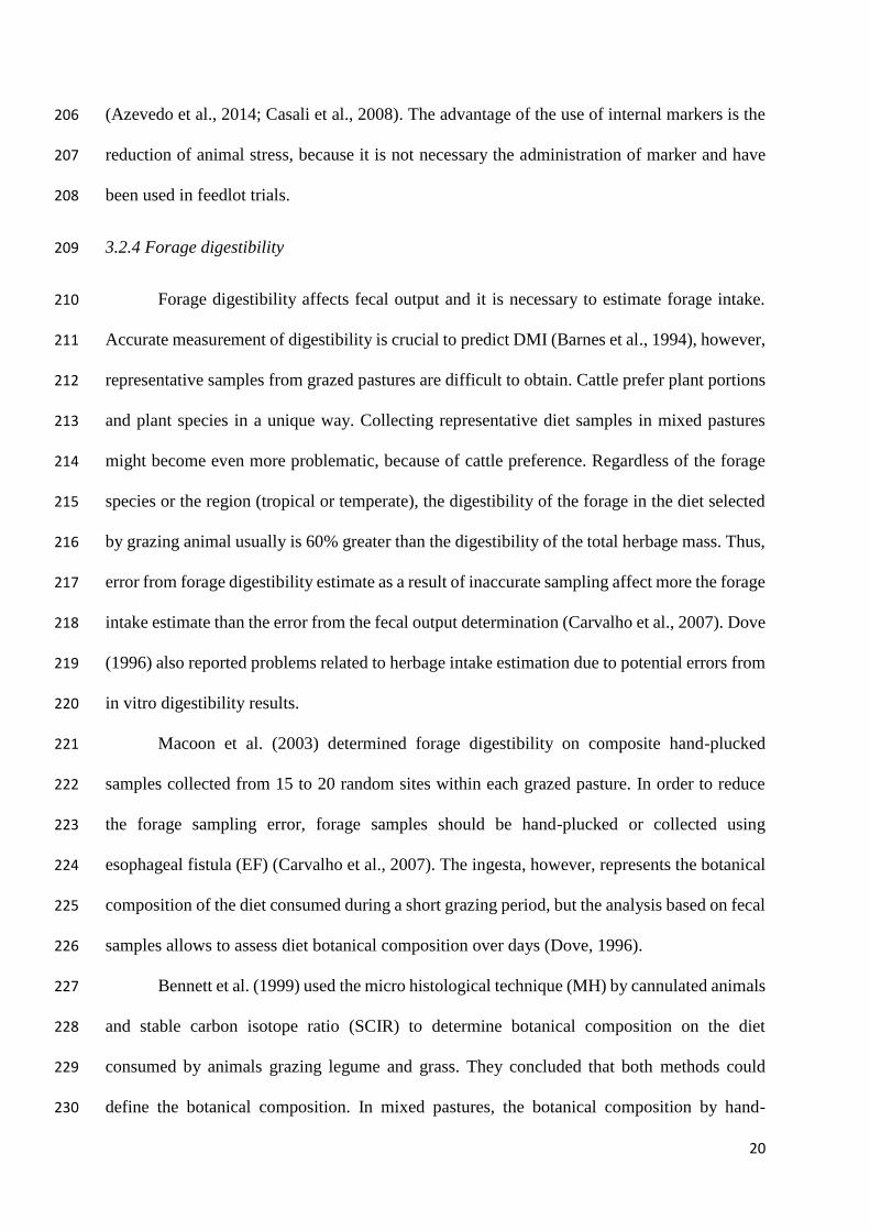
(Azevedo et al., 2014; Casali et al., 2008). The advantage of the use of internal markers is the 206

reduction of animal stress, because it is not necessary the administration of marker and have 207

been used in feedlot trials. 208

3.2.4 Forage digestibility 209

Forage digestibility affects fecal output and it is necessary to estimate forage intake. 210

Accurate measurement of digestibility is crucial to predict DMI (Barnes et al., 1994), however, 211

representative samples from grazed pastures are difficult to obtain. Cattle prefer plant portions 212

and plant species in a unique way. Collecting representative diet samples in mixed pastures 213

might become even more problematic, because of cattle preference. Regardless of the forage 214

species or the region (tropical or temperate), the digestibility of the forage in the diet selected 215

by grazing animal usually is 60% greater than the digestibility of the total herbage mass. Thus, 216

error from forage digestibility estimate as a result of inaccurate sampling affect more the forage 217

intake estimate than the error from the fecal output determination (Carvalho et al., 2007). Dove 218

(1996) also reported problems related to herbage intake estimation due to potential errors from 219

in vitro digestibility results. 220

Macoon et al. (2003) determined forage digestibility on composite hand-plucked 221

samples collected from 15 to 20 random sites within each grazed pasture. In order to reduce 222

the forage sampling error, forage samples should be hand-plucked or collected using 223

esophageal fistula (EF) (Carvalho et al., 2007). The ingesta, however, represents the botanical 224

composition of the diet consumed during a short grazing period, but the analysis based on fecal 225

samples allows to assess diet botanical composition over days (Dove, 1996). 226

Bennett et al. (1999) used the micro histological technique (MH) by cannulated animals 227

and stable carbon isotope ratio (SCIR) to determine botanical composition on the diet 228

consumed by animals grazing legume and grass. They concluded that both methods could 229

define the botanical composition. In mixed pastures, the botanical composition by hand-230

21

plucked samples can be very different from the diet selected by grazing animals, because the 231

animal consumes specific proportions, not represented by hand-plucked samples. Therefore, 232

the use of SCIR have been recommended, once that the proportion of the plant selected by 233

animal is presented in the feces. Dove (1996) reported that SCIR have proved useful to identify 234

plant photosynthetic pathway. Thus, in pasture with a mixture of C3 and C4 plants, in which it 235

is difficult to estimate the animal selectivity, SCIR can be a tool to estimate the botanical 236

composition of the animal diet, using fecal samples. 237

4. Stable Isotopes 238

4.1 Stable Isotope Definition 239

As a reference to the periodic table, the word “isotope” comes from Greek and means 240

that one isotope of an element occupies the same (iso) place (topos) in the periodic table 241

(Dawson and Brooks, 2001; Fry, 2006). Thus, isotopes are defined as the same element that 242

differ in number of neutrons in the nucleus; they can be stable and radioactive (Fry, 2006; 243

Sulzman, 2007). 244

The 13C isotope, for example, has 6 protons and 7 neutrons, while the 12C has 6 protons 245

and 6 neutrons, and both carbon isotopes are used for the same purpose and have the same 246

functions. Therefore, the atomic weight is different, due to the extra neutron. This extra neutron 247

makes the nucleus heavier, but does not affect most of its chemistry (Fry, 2006). The heavier 248

molecules or ions have a stronger bond, so more energy is necessary to break it, and they react 249

slower than the lightest ones (Freitas et al, 2010). 250

4. 2. Isotope Notation 251

The isotope ratios have been expressed by delta (δ) notation, which is the difference, 252

relative to internationally accepted standards (Fry, 2006). Because of the high price, one or 253

more internal working standards are used in the laboratories, which are compared against the 254

22

international standard (Ehleringer and Rundel, 1989; Sulzman 2007). The standard for 255

hydrogen and oxygen is Standard Mean Ocean Water (SMOW), for carbon, it is a fossil, the 256

PeeDee Belemnite (PDB), for nitrogen it is air (AIR) and for sulfur it is Canyon Diablo 257

meteorite (CD) (Ehleringer and Rundel, 1989; Hayes, 2004; Fry, 2006). 258

The δ values are commonly expressed in per mil (‰) (Tcherkez et al., 2011), which is 259

not a unit, but actually a deviation from the ratio of heavy to light isotopes in the sample by the 260

same ratio from the standard, considered to have δ value equal to 0. The symbol ‰ (permil, 261

from the Latin per mille by analogy with per centum, percent, 10-3) is used to simplify, and it 262

implies the factor of 1000, which is equivalent to express either δ -25‰ or δ -0.025 (Farquhar 263

et al., 1989; Dawson and Brooks, 2001; Hayes, 2004). The δ calculation is summarized in the 264

following equation: 265

𝛿𝑀𝐸 = [(𝑅𝑆𝑎𝑚𝑝𝑙𝑒

𝑅𝑆𝑡𝑎𝑛𝑑𝑎𝑟𝑑⁄ ) − 1] ∗ 1000 266

Where E denotes the element, M is the mass of the heavy isotope, R is the ratio of the 267

heavy to light isotope. Thus, the ratio of 13C:12C is expressed as δ13C and 15N:14N becomes δ15N 268

(Ehleringer & Rundel, 1989; Dawson & Brooks, 2001; Crawford et al., 2008). The final δ value 269

is expressed as the amount of the rarest to commonest isotope in the sample, the higher δ values 270

indicate greater proportion of the least common isotope (Dawson et al., 2002). 271

The natural abundance is the range of δ between -100 and +50‰ for natural samples. 272

Samples with greater proportion of the least common isotope in relation to the standard, are 273

commonly referred to as being ‘enriched’, and samples with proportionally less are referred to 274

as ‘depleted’ (Dawson et al., 2002; Fry, 2006; Crawford, 2008). 275

276

277

23

4. 3. Isotope measurement 278

Isotope abundance in any sample, enriched or not, is measured, with precision, using a 279

isotope ratio mass spectrometer (Dawson et al., 2002), after chemical derivatization (Peterson 280

and Fry, 1987; Fernandez et al., 1996). The mass spectrometer was invented by J.J. Thompson 281

in 1910 (Sulzman, 2007), and it is an instrument which generates ions from either inorganic or 282

organic compounds, and separate these ions by their mass-to-charge ratio (m/z), detecting them 283

qualitatively and quantitatively by their respective m/z and abundance (Gross, 2004). Most 284

mass spectrometers can measure only low molecular weight compounds, usually with molecule 285

mass less than 64 (Ehleringer and Rundel 1989). Current-generation isotope ratio mass 286

spectrometers (IRMS) have three or more Faraday cups, positioned to capture specific masses 287

(e.g., 44, 45, 46) simultaneously (Sulzman, 2007). 288

The IRMS is required for accurate detection of small differences and gaseous samples 289

required for the isotopic determinations (Peterson and Fry, 1987; Dawson and Brooks, 2001). 290

The objective of this analysis is to convert a sample quantitatively to a suitable purified gas 291

(typically CO2, N2, or H2) that the IRMS can analyze. These samples are usually organic, which 292

must be initially dried and ground to a fine powder (Michener and Lajtha, 2007), and then 293

combusted until it emerges as a simple gas (Fry, 2006). The samples are introduced into the 294

IRMS via inlet system as a gas, under ambient conditions, where would naturally move into 295

the IRMS by molecular flow and if they were of different masses, fractionation would occur 296

(Dawson & Brooks, 2001). The difference in the signal between the sample and the standard 297

gases is used to calculate the isotope ratio for the sample (Ehleringer and Rundel, 1989). 298

The IRMS consists of an inlet system, an ion source, an analyzer for ion separation, 299

and a detector for ion registration (Brand, 2004). There are two types of IRMS, the dual-inlet 300

(DI-IRMS) which has a higher precision and the continuous flow (CF-IRMS). In the 301

24

continuous flow, it is possible to introduce multiple component samples (atmospheric air, soil, 302

leaves), and obtain isotopic composition for individual elements or compounds within the 303

mixture; all differences between them are in the inlet component (Sulzman, 2007). The DI-304

IRMS requires a skilled operator, takes more time to run one sample than CF-IRMS, and are 305

more expensive (Dawson and Brooks, 2001). Most ecologists currently use dual CN isotope 306

measurement made with elemental analyzers coupled to mass spectrometers (Fry, 2006). 307

4. 4. Isotope samples 308

Many materials can be used, such as wool, blood (Kristensen et al., 2011; Martins et 309

al., 2012; Norman et al., 2009), food (Deniro and Epstein, 1978; Hwang et al., 2007; Martins 310

et al., 2012; Norman et al., 2009), milk (Braun et al., 2013), soil (Hall and Penner, 2013), plant 311

material (Ballentine et al., 1998; Fernandez et al., 2003; Gessler et al., 2008), minerals 312

(Michener and Lajtha, 2007), seawater (Peterson et al.,1985; Fry, 1991), tooth, bone collagen 313

(Sponheimer et al.,2003), and feces (Jones et al., 1979; Botha and Stock, 2005; Hwang et al., 314

2007; Norma et al.,2009; Kristensen et al., 2011; Martins et al.,2012). Many elements have two 315

or more naturally occurring stable isotopes (Crawford et al., 2008) and are used in isotope 316

analysis, such as carbon (C), nitrogen (N), sulfur (S), hydrogen (H) and oxygen (O), where 317

CNS elements are more related to organic matter cycling and HO elements are more related to 318

the hydrological cycle (Fry, 2006). The use of C, N, O, and H to study physiological processes 319

has increased exponentially in the last thirty years (Marshall et al., 2007). 320

4.5. Isotope technique and field analysis 321

Stable isotope chemistry was once the domain of the earth sciences, but the use was 322

largely inaccessible to biologists, due to difficulty with the technique. The situations has 323

changed in the past two decades with the improvement of the tool (Martínez del rio et al., 324

2009). Stable isotopes may serve as potentially useful markers of ecosystem process studies 325

25

(Ehleringer and Rundel, 1989; Brazier, 1997). They might also be useful in studies of animal 326

ecology (Gannes et al., 1997) and geochemistry cycles (Freitas et al., 2010). 327

Access to isotope ratio mass spectrometers has increased and the costs for sample 328

analysis have decreased in recent years. As a result, researchers of different fields have 329

increasingly added stable isotope analysis as additional tool in their investigation (Michener 330

and Lajtha, 2007). Stable isotope analyses have an important contribution to animal ecology 331

and food chains. The foods that animals eat often shows specific isotopic composition (Gannes 332

et al., 1997). Carbon isotopes can be used to back calculate the diet of small ruminants (Norman 333

et al., 2009), cattle (Jones et al., 1979), and wild herbivores (Botha and Stock, 2005). Likewise, 334

15N in feces can be useful to reconstruct animal diet (Hwang et al., 2007) and the sulfur isotope 335

34S as an additional tool for salt marshes and estuaries studies (Peterson et al., 1985). Stable 336

isotopes have been also used to identify sources of pollutants, heterotrophic nitrification, and 337

to estimate rates (e.g. soil C turnover). They can also be used to evaluate models derived from 338

other techniques, to corroborate, reject, or restrict results from other analyses (Sulzman, 2007). 339

5. Carbon Stable Isotopes 340

The carbon cycle is defined by exchanges of CO2 between atmosphere and terrestrial 341

ecosystems (Fry, 2006). In the nature, there are two stable isotopes of carbon, the 12C and 13C; 342

the 12C corresponds to approximately 99% of the total C, while the 13C about 1% (Ludlow et 343

al., 1976; O’Leary et al. 1988, Farquhar et al., 1989). 344

The δ13C of atmospheric CO2 is decreasing due to inputs of depleted CO2 from fossil 345

fuel burning and decomposition (Fry, 2006). In the absence of industrial activity, the δ 13C 346

value of atmospheric CO2 is -8‰ (O’Leary et al.1988). Plants contain less 13C than the 347

atmospheric CO2 on which they depend for photosynthesis; therefore, plants are “depleted” of 348

13C relative to the atmosphere. This occurs because enzymatic and physical processes 349

26

discriminate against 13C in favor of 12C (Marshall et al., 2007; Farquhar et al., 1989). Different 350

discrimination occurs between plant physiological groups. This information can be used to 351

specify plants that use different photosynthetic pathways (O’Leary et al., 1988). Stable carbon 352

isotopes (12C and 13C) at natural abundance is a tool to assess physiological, ecological, and 353

biogeochemical processes related to ecosystems (Tcherkez et al. 2011). 354

5. 1. Stable Isotope Carbon Natural Abundance 355

The C3 plants, that photosynthesize exclusively via the Calvin photosynthetic cycle, 356

and C4 plants that have C4 carbon cycle are different in leaf anatomy (Taiz and Zeiger, 2002) 357

and have different photosynthetic pathways. Therefore, 13C discrimination varies between 358

these two physiological groups (Marshall et al., 2007). Soil organic matter is depleted in 13C 359

compared to atmospheric CO2 and the standard. Ratios are reported in the differential notation 360

relative to the PDB standard (Focken, 2004), that is a Cretaceous belemnite, Belemnitella 361

americana, from the Pee Dee Formation of South Carolina (Craig, 1957; Lerman,1975; Hayes, 362

2004). Because the PDB is no longer available, a new reference standard, Vienna-PDB (VPDB) 363

has been defined (Sulzman, 2007), and recent reports often present values of δVPDB equal to 364

values of δPDB (Hayes, 2004). 365

In the literature, it is possible to find a variety of δ13C signatures. O’Leary et al. (1988) 366

mentioned the δ13C value of C3 near -28‰ and C4 approximately -14‰, while Fernandez et al. 367

(2003) reported the value of C3 ranging from -26‰ to -29‰ and the C4 plants commonly 368

ranging from -12‰ to -14‰. Ballentine et al. (1998) observed a variety of C3 plants with δ13C 369

value ranging from -20‰ to -32‰, and the C4 plants from -9‰ to -17‰. Thus, the 13C 370

composition in photosynthetic products vary between plants species, plant developmental 371

stages, and environmental conditions (Ghashghaie and Tcherkez, 2013). 372

373

27

5. 2. C3 and C4 plants 12C/13C discrimination 374

The atmospheric CO2 is transported through the boundary layer and the stomata into 375

the internal gas space to dissolve in the cell, and then diffuses to the chloroplast, where the 376

carboxylation occurs (O’Leary et al., 1988). The atmospheric CO2 transported is composed of 377

12C and 13C. The intra cell diffusion has an apparent fractionation (Δδ) of about 4.4‰ due to 378

the slower motion of the heavier 13C (Marshall et al., 2007). The atmospheric CO2 379

transportation process is reversible; however, the carboxylation step is irreversible and after 380

this event the isotope fractionation does not change (O’Leary et al.,1988). If diffusion 381

exclusively limits photosynthesis and the stomatal resistance is high, the fractionation would 382

reflect only the diffusive processes, where the Δδ is about 4‰. Whether the diffusion has no 383

limitation, the stomatal diffusion is quick, the fractionation would be equivalent to the 384

enzymatic step, then the Δδ is about 29‰ (Farquhar et al., 1982; O’Leary et al., 1988; Marshall 385

et al., 2007). 386

The CO2 diffusion in air and aqueous solution have a small fractionation, Δδ 4.4 and 387

0.7‰ and the enzyme ribulose bisphosphate carboxylase/oxygenase (rubisco) discriminates 388

against the 13C and with a fractionation of 29‰ (O’Leary et al.,1988; Marshall et al., 2007). In 389

C3 plants, CO2 uptake is more limited by the rate of rubisco than by diffusion (O’Leary et al., 390

1988). The average total organic matter is depleted in 13C by nearly 20‰ compared with 391

atmospheric CO2 (Tcherkez et al., 2011). Thus during photosynthesis, a fractionation of 20‰ 392

occurs between the source atmospheric CO2 at -8‰ and the -28‰ plant sugar product, that is 393

formed from atmospheric CO2 (Fry, 2006). 394

For C4 plants, the Δδ is about 4‰ due to the involvement of the CO2-concentrating 395

mechanism involving the phosphoenolpyruvate carboxylase (PEPc) (Ghashghaie & Tcherkez, 396

2013). The CO2 diffuses through stomata to the mesophyll cells, where it dissolves and is 397

28

converted to bicarbonate (HCO3–), which is in equilibrium with CO2 in 13C concentrations 398

(O’Leary, 1988; Farquhar et al., 1989). Thus, the isotopic fractionation in C4 is the result from 399

the fixation of 13C enriched HCO3 – by PEPc. Therefore, the products from the Calvin cycle 400

simply reflect the net effect of CO2 fixation by the PEPc and are about 4‰ depleted compared 401

with atmospheric CO2 (Tcherkez et al., 2011), thereby the predicted δ 13C value is -12 ‰. The 402

steps that are significant for isotope fractionation are stomatal diffusion and PEPc, where the 403

diffusion is the first limiting in C4 plants (O’Leary,1988). 404

6. Carbon stable isotopes and the reconstruction of animal diets 405

6. 1. Carbon analysis technique for animal diet 406

The carbon stable isotope method is based on fractionation of 13C by plants in the 407

photosynthesis pathway (Botha and Stock, 2005), and has been used to provide a quantitative 408

description of the diet where different sources can be analyzed from a single sampling 409

(Crawford et al., 2008). Diet isotopic composition can be similar as that of animal tissues 410

(Gannes et al., 1997). Materials such as hair, blood, and feces are suitable, due to non-411

destructive collection (Hwang et al., 2007), and provide dietary information with different 412

temporal scale. Fecal samples from animals that are fed with different proportions of C3 and C4 413

plants reflect short-term dietary changes and the collection is easier than plasma samples 414

(Norman et al., 2009), allowing to assess diet selectivity over short-time scales (Botha and 415

Stock, 2005). 416

Fecal δ13C changes within few days of consumption, whereas the changes in hair 417

samples δ13C provides longer-term assessment (Sponheimer et al., 2003a; Martins et al., 2012). 418

Therefore, this technique has been used to study diet selection by animals. Analysis of feces 419

can be an irreplaceable tool for field ecologists to study diet variations (Codron & Codron, 420

29

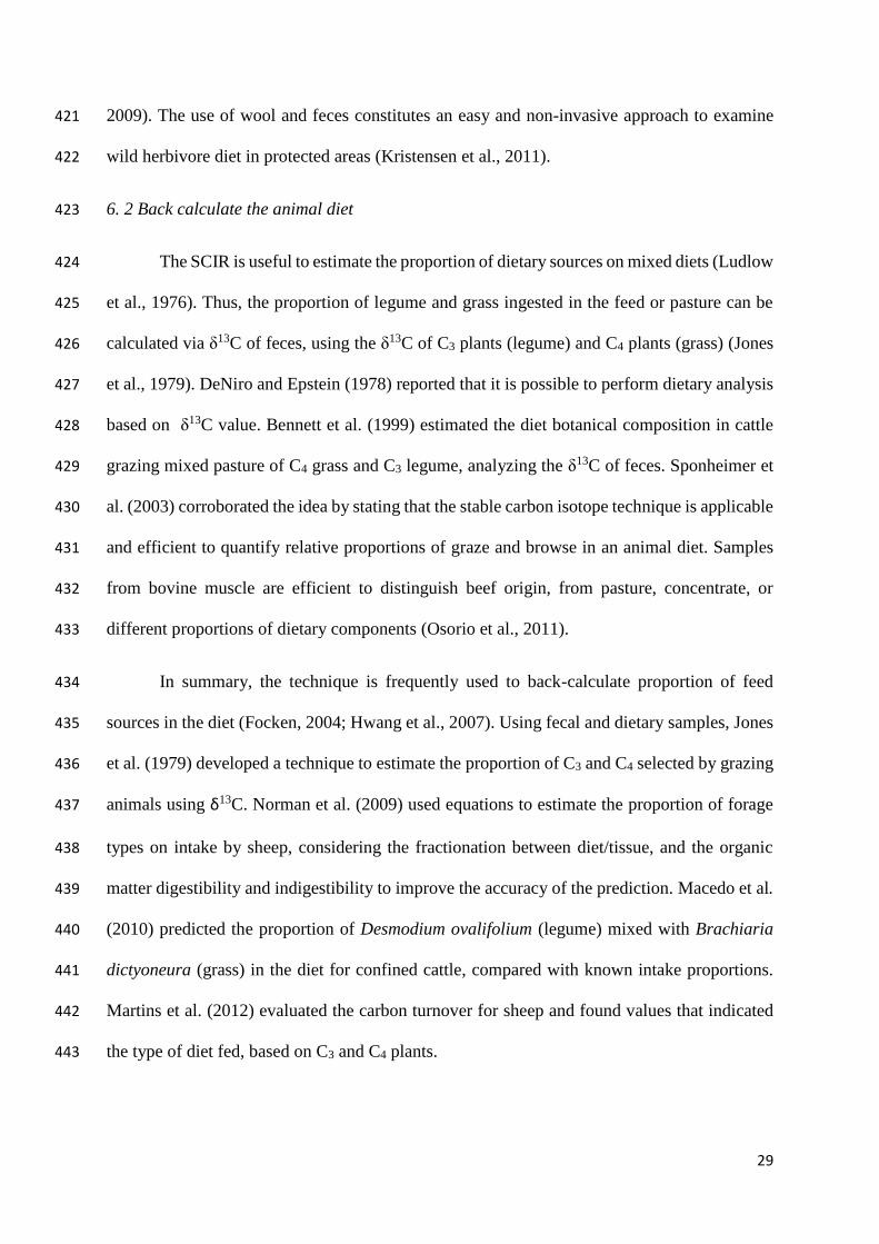
2009). The use of wool and feces constitutes an easy and non-invasive approach to examine 421

wild herbivore diet in protected areas (Kristensen et al., 2011). 422

6. 2 Back calculate the animal diet 423

The SCIR is useful to estimate the proportion of dietary sources on mixed diets (Ludlow 424

et al., 1976). Thus, the proportion of legume and grass ingested in the feed or pasture can be 425

calculated via δ13C of feces, using the δ13C of C3 plants (legume) and C4 plants (grass) (Jones 426

et al., 1979). DeNiro and Epstein (1978) reported that it is possible to perform dietary analysis 427

based on δ13C value. Bennett et al. (1999) estimated the diet botanical composition in cattle 428

grazing mixed pasture of C4 grass and C3 legume, analyzing the δ13C of feces. Sponheimer et 429

al. (2003) corroborated the idea by stating that the stable carbon isotope technique is applicable 430

and efficient to quantify relative proportions of graze and browse in an animal diet. Samples 431

from bovine muscle are efficient to distinguish beef origin, from pasture, concentrate, or 432

different proportions of dietary components (Osorio et al., 2011). 433

In summary, the technique is frequently used to back-calculate proportion of feed 434

sources in the diet (Focken, 2004; Hwang et al., 2007). Using fecal and dietary samples, Jones 435

et al. (1979) developed a technique to estimate the proportion of C3 and C4 selected by grazing 436

animals using δ13C. Norman et al. (2009) used equations to estimate the proportion of forage 437

types on intake by sheep, considering the fractionation between diet/tissue, and the organic 438

matter digestibility and indigestibility to improve the accuracy of the prediction. Macedo et al. 439

(2010) predicted the proportion of Desmodium ovalifolium (legume) mixed with Brachiaria 440

dictyoneura (grass) in the diet for confined cattle, compared with known intake proportions. 441

Martins et al. (2012) evaluated the carbon turnover for sheep and found values that indicated 442

the type of diet fed, based on C3 and C4 plants. 443

30

Likewise, Focken (2004) back-calculated the proportion of mixed diet of fish 444

(controlled condition) via linear interpolation between the fish on the two sources used, 445

compared to the condition in which it was applied individually. Bruckental et al. (1985) 446

determined the digestibility of hay (C3) and grain (C4), individually, used to feed rams in 447

different proportions of the diet, using fecal δ13C value. 448

6. 3. Difference between dietary and animal tissue δ13C 449

The isotopic reconstruction of the diet from δ13C value from animal tissue or feces is 450

based on the hypothesis that there is a known constant relationship between the δ13C of the 451

forage and the tissue or feces (Wittmer et al., 2010). Norman et al. (2009) found a positive 452

relationship between δ13C values of samples, such as feces, plasma, rumen solids, rumen liquor, 453

urine and wool and the δ13C of the diet. However, the animal isotopic signal incorporation rate 454

from the diet differs among organisms and tissue, individually (Martínez Del Rio et al., 2009; 455

Wolf et al., 2009). Different digestibility or fractionation during assimilation and metabolic 456

processes can change the stable isotopic relationship between diet and animal (tissue) (Gannes 457

et al. 1997; McCutchan Jr et al. 2003, and DeNiro and Epstein 1978). This relationship depends 458

on both the type of tissue and the nature of the diet. The accuracy of this relation is limited by 459

the seasonal variation of δ13C of the diet, and the random intake of plants in the field (DeNiro 460

and Epstein 1978). 461

6. 3. 1. Diet-animal sample discrimination 462

The isotopic difference between tissue and diet is known as tissue-diet discrimination, 463

and is presented as Δ (Δ = δ tissue – δ diet) (Wolf et al., 2009). Some authors present the 464

calculations, models or expression based on tissue, but this can be also applied to feces (Jones 465

et al., 1976; Botha and Stock, 2005; Hwang et al., 2007; Norma et al., 2009; Kristensen et al., 466

2011; Martins et al., 2012), ruminal fluid (Norman et al., 2009), and breath (CO2) (Ayliffe et 467

31

al., 2004; Passey et al., 2005). The δ13C information is related to the type of animal sample or 468

product analyzed; for instance, feces or samples from gut represent the diet information in a 469

short-time scale, while animal tissue represents the long-term scale (Tieszen et al., 1983). 470

The relationship determined by DeNiro and Epstein (1978) between the δ13C of the 471

animal and the diet ingested, was about 1‰ compared with the diet, where the δ13C value 472

obtained from the whole animal was considered enriched. Wittmer et al. (2010) assessed the 473

relationship among forage, feces, and wool of sheep under grazing. They found that the δ13C 474

of feces and diet was 0.6‰, feces and wool -4.3‰, as well as wool and diet -3.9‰. In feces, 475

Jones et al. (1976) obtained -0.4 (grass) and -2.0 ‰ (legume) for δ13C between herbivore diets 476

and fecal samples. Sponheimer et al. (2003) also examined the δ13C of diet-feces for herbivores 477

fed with alfalfa and bermudagrass (Cynodon dactylon) and observed the mean δ13C of -0.8‰ 478

for both diets, where the alfalfa (-0.6‰) δ13C was less depleted than bermudagrass (-1.0‰). 479

The δ13C diet-feces found by Norman et al. (2009) was -0.94‰ for sheep fed on plants with C3 480

and C4 photosynthetic pathways. 481

Some authors have assumed this discrimination as constant to estimate the proportion 482

of different sources in the diet (e.g., Sponheimer et al., 2003; Codron et al., 2007, 2011; Norman 483

et al, 2009). The diet–tissue discrimination factors can vary. Thus, using fixed discrimination 484

factors, and (or) discrimination factors that are not diet-dependent, obtained from literature, 485

might result in error in the determination of mixed diet composition (Caut et al., 2008). 486

6. 3. 2. Fecal endogenous contamination 487

The variation between δ13C value of feces and diet might also be explained by 488

endogenous contamination, as tissue or fluid from the gut is expelled and results in an over-489

estimation of the quantity of a source in the diet, due to the fact that the δ13C is different (more 490

depleted) from the δ13C value ingested (Jones et al., 1976). Thus, contamination of the feces 491

32

by endogenous material could be related with the discrimination diet-feces (Martins et al. 492

2012). The fecal is composed mainly of bacterial and some endogenous matter (Van Soest, 493

1994). Sponheimer et al. (2003) found a negative fractionation between feces and herbivores 494

diet, where feces had a greater proportion of acid detergent fiber, enriched in 13C, compared 495

with the diet. They expected a δ13C value more positive, but assuming that after the use of acid 496

detergent the microbiota was removed from feces, the δ13C value should increase, therefore, 497

the hypothesis of the influence of microbiota was not supported. 498

6. 3. 3 Different digestibility and δ13C of animal diet 499

Different plant digestibility that are part of the animal diet can be related also with the 500

δ13C value between diet and feces (Jones et al., 1979). The δ13C diet-feces is influenced by the 501

difference between the digestibility of the mixed diet, where the less digestible component is 502

overestimated in the feces (Botha and Stock, 2005). Norman et al. (2009) classified the 503

difference in the organic matter digestibility of the C3 and C4 components of the diet as one of 504

the possible factors that contribute to errors in diet reconstruction, and the use of digestibility 505

can improve the accuracy of the method. However, Wittmer et al. (2010) did not find influence 506

of different digestibility of C3 and C4 species, for grazing animals. Thus, the different 507

digestibility of sources did not affect the diet reconstruction from fecal δ13C values 508

(Sponheimer et al., 2003). 509

7. Discrimination of δ13C in different plant tissue 510

In general, the analysis of δ13C values are made on leaves, however, there are variation 511

in δ13C value among organs in the plants (O’leary, 1981). This variation is caused due to genetic 512

and environment factors, linked with gas exchange by morphological and plant responses 513

(Dawson et al., 2002). The tissues that are photosynthetic inefficient, such as stems and roots, 514

are more enriched in 13C than leaf tissue (O’Leary, 1988). In normal conditions, Ramírez et al. 515

33

(2015) found a δ13C over 2‰ of leaves and tuber of three genotypes of potato. Differences 516

among chemical components of plant tissue also influence the δ13C of plants, as lignin that is 517

1- 2 ‰ lighter than the total plant (Marshall et al., 2007). Fernandez et al. (2003) observed that 518

the lignin is depleted in 13C compared to cellulose. 519

Difference in the δ13C between lipid and the bulk material ranges from 5 to 10‰, being 520

the lipid depleted in 13C (O’leary, 1981). Ballentine et al. (1998) in a study with three C4 plant 521

genotypes found a discrimination between whole plant and lipid of sugar cane δ13C of 5‰; in 522

Cenchrus ciliaris the discrimination was 7‰ and in Antephoras pubescence it was 9‰. 523

Sponheimer et al. (2003) evaluated the discrimination between plant material and acid-524

detergent fiber (ADF) in Cynodon dactylon and found -1.4 ‰, while alfalfa did not show 525

significant difference. Thus, it is clear that different parts, compound and nutrients of a plant 526

express a particular δ13C value. 527

528

References 529

Allen, V.G., Batello, C., Berretta, E.J., Hodgson, J., Kothmann, M., Li, X., McIvor, J., Milne, 530 J., Morris, C., Peeters, A., Sanderson, M., 2011. An international terminology for 531

grazing lands and grazing animals. Grass Forage Sci. 66, 2–28. 532

Ayliffe, L.K., Cerling, T.E., Robinson, T., West, A.G., Sponheimer, M., Passey, B.H., 533 Hammer, J., Roeder, B., Dearing, M.D., Ehleringer, J.R., 2004. Turnover of carbon 534 isotopes in tail hair and breath CO2 of horses fed an isotopically varied diet. Oecologia 535

139, 11–22. 536

Azevedo, E.B., Poli, C.H.E.C., David, D.B., Amaral, G.A., Fonseca, L., Carvalho, P.C.F., 537

Fischer, V., Morris, S.T., 2014. Use of faecal components as markers to estimate intake 538 and digestibility of grazing sheep. Livest. Sci. 165, 42–50. 539

Ballentine, D.C., Macko, S.A., Turekian, V.C., 1998. Variability of stable carbon isotopic 540

compositions in individual fatty acids from combustion of C 4 and C 3 plants: 541 implications for biomass burning. Chem. Geol. 151–161. 542

Baumont, R., Prache, S., Meuret, M., Morand-Fehr, P., 2000. How forage characteristics 543 influence behaviour and intake in small ruminants: A review. Livest. Prod. Sci. 64, 15–544 28. 545

Bennett, L.L., Hammond, A.C., Williams, M.J., Chase, C.C., Kunkle, W.E., 1999. Diet 546

34

selection by steers using microhistological and stable carbon isotope ratio analyses. J. 547

Anim. Sci. 77, 2252–2258. 548

Benvenutti, M.A., Coates, D.B., Bindelle, J. , Poppi, D.P., Gordon, I.J., 2014. Can faecal 549 markers detect a short term reduction in forage intake by cattle? Anim. Feed Sci. 550 Technol. 194, 44–57. 551

Botha, M.S., Stock, W.D., 2005. Stable isotope composition of faeces as an indicator of 552

seasonal diet selection in wild herbivores in Southern Africa. S. Afr. J. Sci. 101, 371–553 374. 554

Brand, W. A, 2004. Mass spectrometer hardware for analyzing stable isotope ratios, in: 555

Groot, P. A. (Eds.), Handbook of stable isotope analytical techniques, volume-I, Elsevier 556 Science, pp. 835–858. 557

Braun, A., Schneider, S., Auerswald, K., Bellof, G., Schnyder, H., 2013. Forward modeling 558

of fluctuating dietary13C signals to validate13C turnover models of milk and milk 559 components from a diet-switch experiment. PLoS One 8. 560

Brazier, J.L., 1997. Alternative to mass spectrometry for quantitating stable isotopes: Atomic 561 emission detection, in: Stable isotopes in pharmaceutical research. 169–202. 562

Bruckental, B.Y.I., Halevi, A., Amir, S., Neumark, H., 1985. The ratio of naturally occurring 563

13 C and 12 C isotopes in sheep diet and faeces as a measurement for direct 564 determination of lucerne hay and maize grain digestibilities in mixed diets. J. Anim. Sci. 565 104, 271-274. 566

Butler, T.J., Biermacher, J.T., Kering, M.K., Interrante, S.M., 2012. Production and 567

economics of grazing steers on rye-annual ryegrass with legumes or fertilized with 568 nitrogen. Crop Sci. 52, 1931–1939. 569

Burns, J. C., K. R. Pond, D. S. Fisher., 1994. Measurement of Forage Intake. In: G. C. Fahey, 570 editor, Forage Quality, Evaluation, and Utilization, ASA, CSSA, SSSA, Madison, WI. pp. 571 494-532 572

Cadisch, G., Schunke, R.M., Giller, K., 1994. Nitrogen cycling in a pure grass pasture and a 573 grass-legume misture on a red latosol in Brazil. Trop. Grasslands. 28, 43–52 574

Cantarutti, R.B., Tarré, R., Macedo, R., Cadisch, G., Rezende, C.D., Pereira, J.M., Braga, 575 J.M., Gormide, J.A., Ferreira, E., Alves, B.J.R., Urquiaga, S., Boddey, R.M., 2002. The 576

effect of grazing intensity and the presence of a forage legume on nitrogen dynamics in 577 Brachiaria pastures in the Atlantic forest region of the south of Bahia, Brazil. Nutr. Cycl. 578

Agroecosystems 64, 257–271. 579

Carvalho, P.C. de F., Kozloski, G.V., Filho, H.M.N.R., Reffatti, M.V., Genro, T.C.M., 580 Euclides, V.P.B., 2007. Advances in methods for determining animal intake on pasture. 581 Rev. Bras. Zootec. 36, 151–170. 582

Casali, A.O., Detmann, E., Valadares Filho, S.D.C., Pereira, J.C., Henriques, L.T., De 583 Freitas, S.G., Paulino, M.F., 2008. Influência do tempo de incubação e do tamanho de 584 partículas sobre os teores de compostos indigestíveis em alimentos e fezes bovinas 585 obtidos por procedimentos in situ. Rev. Bras. Zootec. 37, 335–342. 586

Caut, S., Angulo, E., Courchamp, F., 2008. Caution on isotopic model use for analyses of 587 consumer diet. Can. J. Zool. 86, 438–445. 588

35

Codron, D., Codron, J., 2009. Reliability of δ13C and δ15N in faeces for reconstructing 589

savanna herbivore diet. Mamm. Biol. 74, 36–48. 590

Craig, H., 1957. Isotopic standards for carbon and oxygen and correction factors for mass 591 spectrometric analysis of carbon dioxide. Geochim. Cosmochim. Acta 12, 133–149. 592

Crawford, K., Mcdonald, R., Bearhop, S., 2008. Applications of stable techiques to the 593 ecology of mammals. Mammal Rev. 38, 87–107. 594

Dawson, T.E., Brooks, P.D., 2001. Fundamentals of stable isotope chemistry and 595 measurement, in: Stable Isotope Techniques in the Study of Biological Processes and 596 Functioning of Ecosystems. pp. 1-18. 597

Dawson, T.E., Mambelli, S., Plamboeck, A.H., Templer, P.H., Tu, K.P., 2002. Stable 598 isotopes in plant ecology. Annu. Rev. Ecol. Syst. 33, 507-559. 599

De Deyn, G.B., Shiel, R.S., Ostle, N.J., Mcnamara, N.P., Oakley, S., Young, I., Freeman, C., 600 Fenner, N., Quirk, H., Bardgett, R.D., 2011. Additional carbon sequestration benefits of 601

grassland diversity restoration. J. Appl. Ecol. 48, 600-608. 602

DeNiro, M.J., Epstein, S., 1978. Influence of diet on the distribution of carbon isotopes in 603

animals. Geochim. Cosmochim. Acta. 425, 495-506. 604

Dove, H., 1996. Constraints to the modelling of diet selection and intake in the grazing 605 ruminant. Aust. J. Agric. Res. 47, 257-275. 606

Dove, H., Mayes, R.W., 2005. Using n-alkanes and other plant wax components to estimate 607

intake, digestibility and diet composition of grazing/browsing sheep and goats. Small 608 Rumin. Res. 59, 123–139. 609

Dubeux Jr, J. C. B., Sollenberger, L. E., Silva, H. M., de Souza, T. C., Mozley III, E. L., & 610

Santos, E. R. S., 2014. Nutrient cycling in tropical pastures: what do we know. In 7th 611

Symposium on Strategic Management of Pasture/5th International Symposium on Animal 612

Production Under Grazing. Visconde do Rio Branco: Suprema pp. 253-286. avalible 613

https://www.researchgate.net/profile/Jose_Dubeux_Jr/publication/280155938_Nutrient_614

Cycling_in_Tropical_Pastures_What_do_we_know/links/55ad109208aed9b7dcd9b1fa/N615

utrient-Cycling-in-Tropical-Pastures-What-do-we-know.pdf (09.12.17) 616

Ehleringer, J.R., Rundel, P.W., 1989. Stable isotopes: History, units, and instrumentation, in: 617 stable isotopes in ecological research (ecological studies 68). pp. 1–16. 618

Farquhar, G.D., Ehleringer, J.R., Hubidk, K.T., 1989. Carbon isotope discrimination and 619 photosynthesis. Annu. Rev. Plant Physiol. 40, 503–537. 620

Fernandez, C. a, Des Rosiers, C., Previs, S.F., David, F., Brunengraber, H., 1996. Correction 621 of 13C mass isotopomer distributions for natural stable isotope abundance. J. Mass 622

Spectrom. 31, 255–62. 623

Fernandez, I., Mahieu, N., Cadisch, G., 2003. Carbon isotopic fractionation during 624 decomposition of plant materials of different quality. Global Biogeochem. Cycles 17, 625 1075. 626

Focken, U., 2004. Feeding fish with diets of different ratios of C3-and C 4-plant-derived 627 ingredients: A laboratory analysis with implications for the back-calculation of diet from 628 stable isotope data. Rapid Commun. Mass Spectrom. 18, 2087–2092. 629

36

Forbes, J. M., Gregorini, P., 2015. The catastrophe of meal eating. Anim. Prod. Sci. 55, 350–630

359. 631

Freitas, A.D.S.S., E.V.S.B., Santos, C.E. R.S., 2010. Abundância natural do 15 N para 632 quantificação da fixação biológica do nitrogênio em plantas, in: Figueiredo, M. V. B; 633 Burity, H. A; Oliveira, J. P; Santos, C. E. R. S; Stamford, N. P. Biotecnologia aplicada à 634 agricultura: textos de apoio e protocolos experimentais. EMBRAPA, Brasilia, pp. 505-635 517. 636

Fry, B., 2006. Stable isotope ecology. Springer Science & Business Media 637

Gannes, L.Z., O’Brien, D.M., Martínez del Rio, C., 1997. Stable isotopes in animal ecology : 638

Assumptions , caveats , and a call for more laboratory experiments. Ecology 78, 1271–639 1276. 640

Gessler, A., Tcherkez, G., Peuke, A.D., Ghashghaie, J., Farquhar, G.D., 2008. Experimental 641

evidence for diel variations of the carbon isotope composition in leaf, stem and phloem 642 sap organic matter in Ricinus communis. Plant, Cell Environ. 31, 941–953. 643

Givens, D. I., Owen, E., Axford, R. F. E., Omed, H. M., 2000. Forage evaluation in ruminant 644 nutrition. Uk. Cabi. pp. 449. 645

Ghashghaie, J., Tcherkez, G., 2013. Isotope ratio mass spectrometry technique to follow plant 646

metabolism. Principles and applications of 12C/13C isotopes, 1st ed, Advances in 647 Botanical Research. Elsevier Ltd. 648

Gregorini, P; Villalba, J. J; Provenza, F. D; Beukes, P. C; Forbes, J. M., 2015. Modelling 649 preference and diet selection patterns by grazing ruminants: a development in a 650

mechanistic model of a grazing dairy cow, MINDY. Anim. Prod. Sci. 55, 360-375. 651

Gross, J.H., 2004. Mass Spectometry. pp. 1–12. 652

Hall, S.A., Penner, W.L., 2013. Stable carbon isotopes, C3-C4 vegetation, and 12,800years of 653

climate change in central New Mexico, USA. Palaeogeogr. Palaeoclimatol. Palaeoecol. 654 369, 272–281. 655

Hayes, J.M., 2004. An introduction to isotopic calculations. At. Energy 1–10. 656

Hwang, Y.T., Millar, J.S., Longstaffe, F.J., 2007. Do δ 15 N and δ 13 C values of feces 657 reflect the isotopic composition of diets in small mammals? Can. J. Zool. 85, 388–396. d 658

Jones, R.J., Ludlow, M.M., Troughton, J.H., G, B.C., 1979. Estimating eaten C3 and C4 from 659 feaces. J. Agric. Sci. 91–100. 660

Kristensen, D.K., Kristensen, E., Forchhammer, M.C., Michelsen, A., Schmidt, N.M., 2011. 661

Arctic herbivore diet can be inferred from stable carbon and nitrogen isotopes in C-3 662 plants, faeces, and wool. Can. J. Zool. Can. Zool. 89, 892–899. doi:Doi 10.1139/Z11-663

073 664

Laca, E.A., Wallis De Vries, M.F., 2000. Acoustic measurement of intake and grazing 665

behaviour of cattle. Grass Forage Sci. 55, 97–104. 666

Ledgard, S.F., Steele, K.W., 1992. Biological nitrogen-fixation in mixed legume grass 667 pastures. Plant Soil 141, 137–153. 668

Ledgard, S. F., 2001. Nitrogen cycling in low input legume-based agriculture, with emphasis 669 on legume/grass pastures. Plant Soil 288, 43-59. 670

37

Lerman, J. C., 1975. How to interpret variations in the carbon isotope ratio of plants: biologic 671

and environmental effects, in: R. Marcelle (Eds), Environmental and Biological Control 672 of Photosynthesis, Dr. W. Junk b.v., Publishers, The Hague, pp. 323-335 673

Lira, M.A., Santos, M.V.F., Dubeux Jr., J.C.B., Lira Jr., M.A., Mello, A.C.L. , 2006. Sistemas 674 de produção de forragem: Alternativas para sustentabilidade da pecuária. Rev. Bras. 675 Zootec. 35, 491 - 511. 676

Ludlow, M.M., Troughton, J.H., Jones, R.J., 1976. A technique for determining the 677 proportion of C3 and C4 species in plant samples using stable natural isotope’s of carbon. 678 J. Agric. Sci. 87, 625–632. 679

Lüscher, A., Mueller-Harvey, I., Soussana, J. F., Rees, R. M., Peyraud, J. L., 2014. Potential 680 of legume-based grassland–livestock systems in Europe: a review. Grass Forage Sci. 69, 681 206-228. 682

Macedo, R., Tarré, R., Ferreira, E., De Paula Rezende, C., Marques Pereira, J., Cadish, G., 683 Ribeiro, J. C. R, Rodrigues, B. A., Boddey, R., 2010. Forage intake and botanical 684

composition of feed for cattle fed Brachiaria/legume mixtures. Sci. Agric. 67, 384–392. 685

Macoon, B., Sollenberger, L.E., Moore, J.E., Staples, C.R., Fike, J.H., Portier, K.M., 2003. 686 Comparison of three techniques for estimating the forage intake of lactating dairy cows 687

on pasture. J. Anim. Sci. 81, 2357–2366. 688

Marshall, J. D; Brooks, J. R; Lajtha, K., 2007. Sources of variation in the stable isotopic 689 composition of plants, in: Michener, R.; Lajtha, K. (Eds), Stable isotopes in ecology and 690

environmental science. 2nd. ed. Oxford: Blackwell, p. 22-50. 691

Martínez Del Rio, C., Wolf, N., Carleton, S.A., Gannes, L.Z., 2009. Isotopic ecology ten 692 years after a call for more laboratory experiments. Biol. Rev. 84, 91–111. 693

Martins, M.B., Ducatti, C., Martins, C.L., Denadai, J.C., Natel, A.S., Souza-Kruliski, C.R., 694 Sartori, M.M.P., 2012. Stable isotopes for determining carbon turnover in sheep feces 695 and blood. Livest. Sci. 149, 137–142. 696

McCutchan Jr, J.H., Lewis Jr, W.M., Kendall, C., McGrath, C.C., 2003. Variation in trophic 697 shift for stable isotope ratios of carbon, nitrogen, and sulfur. Oikos 102, 378–390. 698

Mertens, D. R.,1994. Regulation of Forage Intake, in: Fahey,G. C., (Eds), Forage quality, 699 evaluation, and utilization, ASA, CSSA, SSSA, Madison, pp. 450-493. 700

Mertens, D. R., 2007. Digestibility and Intake, in: Barnes, R. F; Nelson, C. J; Moore, K. J; 701

Collins, M. (Eds), Forages, volume II: The science of grassland agriculture, 6th edition. 702 Wiley-Blackwell, pp.808 703

Michener, R., Lajtha, K., 2007. Stable isotopes in ecology and environmental science, 2nd ed. 704 Blackwell, Oxford. 705

Minson, D.J., 1990. Forage in ruminant nutrition San Diego: Academic Press, pp. 483. 706

Minson, D.J., J. R. Wilson., 1994. Prediction of Intake as an Element of Forage Quality, in: 707 Fahey,G. C., (Eds), Forage Quality, Evaluation, and Utilization, ASA, CSSA, SSSA, 708

Madison, pp. 533-563. 709

Muir, J.P., Pitman, W.D., Foster, J.L., 2011. Sustainable, low-input, warm-season, grass-710 legume grassland mixtures: mission (nearly) impossible? Grass Forage Sci. 66, 301–711

38

315. 712

Muir, J.P., Pitman, W.D., Foster, J.L., 2014. The future of warm-season, tropical and 713

subtropical forage legumes in sustainable pastures and rangelands. Afri. J. Range. 714 Forage. Sci. 31, 1-12. 715

Nyfeler, D., Huguenin-Elie, O. Suter, M., Frossard, E., Lüscher, A., 2011. Grass-legume 716 mixtures can yield more nitrogen than legume pure stands due to mutual stimulation of 717

nitrogen uptake from symbiotic and non-symbiotic sources. Agric. Ecosyst. Environ. 718 140, 155-163. 719

Norman, H.C., Wilmot, M.G., Thomas, D.T., Masters, D.G., Revell, D.K., 2009. Stable 720

carbon isotopes accurately predict diet selection by sheep fed mixtures of C3 annual 721 pastures and saltbush or C4 perennial grasses. Livest. Sci. 121, 162–172. 722

O’Leary, M.H., 1981. Carbon isotope fractionation in plants. Phytochemistry 20, 553–567. 723

O’Leary, M.H., 1988. Carbon isotopes in photosynthesis. BioSciencie 38, 328-336. 724

Oltjen, J.W., Gunter, S.A., 2015. Managing the herbage utilisation and intake by cattle 725 grazing rangelands. Anim. Prod. Sci. 55, 397–410. 726

Osorio, M.T., Moloney, A.P., Schmidt, O., Monahan, F.J., 2011. Beef authentication and 727

retrospective dietary verification using stable isotope ratio analysis of bovine muscle and 728 tail hair. J. Agric. Food Chem. 59, 3295–3305. 729

Passey, B.H., Robinson, T.F., Ayliffe, L.K., Cerling, T.E., Sphonheimer, M., Dearing, M.D., 730

Roeder, B.L., Ehleringer, J.R., 2005. Carbon isotope fractionation between diet, breath 731 CO2, and bioapatite in different mammals. J. Archaeol. Sci. 32, 1459–1470. 732

Peterson, B., Fry, B., 1987. Stable isotopes in ecosystem studies. Annu. Rev. Ecol. Syst. 18, 733

293–320. 734

Peterson, B.J., Howarth, R.W., Garritt, R.H., 1985. Multiple stable isotopes used to trace the 735 flow of organic matter in estuarine food webs. Science (80-. ). 227, 1361–1363. 736

Ramírez, D.A., Rolando, J.L., Yactayo, W., Monneveux, P., Quiroz, R., 2015. Is 737

discrimination of 13c in potato leaflets and tubers an appropriate trait to describe 738 genotype responses to restrictive and well-watered conditions? J. Agron. Crop Sci. 201, 739 410–418. 740

Redmon, L. A; Hendrickson J. R., 2007. Forage Systems for Temperate Subhumid and 741 Semiarid Areas, In: Barnes, R. F; Nelson, C. J; Moore, K. J; Collins, M. (Eds), Forages, 742 volume II: The Science of Grassland Agriculture, 6th Edition. Iowa, Wiley-Blackwell, 743 pp.808 744

Rochon, J.J., Doyle, C.J., Greef, J.M., Hopkins, A., Molle, G., Sitzia, M., Scholefield, D., 745

Smith, C.J., 2004. Grazing legumes in Europe: A review of their status, management, 746 benefits, research needs and future prospects. Grass Forage Sci. 59, 197–214. 747

Rótolo, G.C., Rydberg, T., Lieblein, G., Francis, C., 2007. Energy evaluation of grazing 748 cattle in Argentina’s Pampas. Agric. Ecosyst. Environ. 119, 383–395. 749

Rotz, C.A., Taube, F., Russelle, M.P., Oenema, J., Sanderson, M.A., Wachendorf, M., 2005. 750 Whole-farm perspectives of nutrient flows in grassland agriculture. Crop Sci. 45, 2139–751 2159. 752

39

Schlesinger, W.H., 2009. On the fate of anthropogenic nitrogen. Proc. Natl. Acad. Sci. 106, 753

203–208. 754

Sleugh, B., Moore, K.J., George, J.R., Brummer, E.C., 2000. Binary legume-grass mixture 755 improve forage yield, quality, and seasonal distribution. Agron. J. 92, 24–29. 756

Sponheimer, M., Lee-Thorp, J.A., Deruiter, D.J., Smith, J.M., Van Der Merwe, N.J., Reed, 757 K., Grant, C.C., Ayliffe, L.K., Robinson, T.F., Heidelberger, C., Marcus, W., 2003a. 758

Diets of southern african bovidae : stable isotope evidence. J. Mammal. 84, 471–479. 759

Sponheimer, M., Robinson, T., Ayliffe, L., Passey, B., Roeder, B., Shipley, L., Lopez, E., 760 Cerling, T., Dearing, D., Ehleringer, J., 2003b. An experimental study of carbon-isotope 761

fractionation between diet, hair, and feces of mammalian herbivores. Can. J. Zool. 81, 762 871–876. 763

Sulzman, E. W., 2007. Stable isotope chemistry and measurement: a primer, in: Michener, R.; 764

Lajtha, K. editors, Stable isotopes in ecology and environmental science. 2nd. ed. Oxford: 765 Blackwell, p. 1-18. 766

Taiz, L. and Zeiger, E., 2002. Plant physiology. Plant Physiol. 91, 690. 767

Tcherkez, G., Mahé, A., Hodges, M., 2011. 12C/13C fractionations in plant primary 768 metabolism. Trends Plant Sci. 16, 499–506. 769

Tieszen, L.L., Boutton, T.W., Tesdahl, K.G., Slade, N.A., 1983. Fractionation and turnover 770 of stable carbon isotopes in animal tissues: Implications for δ13C analysis of diet. 771

Oecologia 57, 32–37. 772

Van Soest, Peter J., 1994. Nutritional ecology of the ruminant. Ithaca, Cornell University Press 773

Vendramini, J.M.B., Silveira, M.L.A., Dubeux Jr., J.C.B., Sollenberger, L.E., 2007. 774

Environmental impacts and nutrient recycling on pastures grazed by cattle. Rev. Bras. 775 Zootec. 36, 139–149. 776

White, R., Rohweder, M., Murray, S., 2000. Pilot Analysis of Global Ecosystems: Grassland 777

Ecosystems, Pilot Analysis of Global Ecosystems. 778

Wittmer, M.H.O.M., Auerswald, K., Schönbach, P., Schäufele, R., Müller, K., Yang, H., Bai, 779 Y.F., Susenbeth, A., Taube, F., Schnyder, H., 2010. Do grazer hair and faeces reflect the 780 carbon isotope composition of semi-arid C3/C4 grassland? Basic Appl. Ecol. 11, 83–92. 781

Wolf, N., Carleton, S.A., Martínez del Rio, C., 2009. Ten years of experimental animal 782 isotopes ecology. Funct. Ecol. 23, 17–26. 783

784

785

786

787

788

789

790

40

791

792

793

794

795

796

797

798

799

Chapter 2 800

Tracing back ruminant diet feeding grass-legume mixtures using fecal δ 13C 801

802

803

804

805

806

807

808

809

810

811

812

813

814

815

816

817

818

41

Resumo 819

Os isótopos estáveis podem ser uma importante ferramenta de pesquisa para rastrear C e N em 820

experimentos de pastagem. Este estudo testou diferentes proporções de gramineas C4 e 821

leguminosa e a correlação entre δ13C dietético com δ13C fecal. Quarenta cordeiros, com peso 822

corporal médio de 20,4 kg, foram casualizados em blocos e alimentados com feno de Tifton-823

85 (Cynodon spp.) e Alfafa (Medicago sativa), em diferentes níveis de substituição, compondo 824

cinco tratamentos: 1) 100% de Tifton -85 feno; 2) 75% de Tifton-85 + 25% de feno de alfafa; 825

3) 50% de Tifton-85 + 50% de feno de alfafa; 4) 75% de alfafa + 25% de feno Tifton-85; 5) 826

100% feno de feno de alfafa. O experimento durou 27 dias, consistindo de 22 dias para a 827

adaptação e 5 dias para a coleta de sobras, alimentos e fezes. As amostras fecais foram coletadas 828

diretamente do reto, para evitar contaminação. Todas as amostras foram coletadas durante o 829

período de amostragem de 5 dias, sendo composta no final. As amostras de alimentação e fezes 830

foram secas por 72 horas em uma estufa (55ºC) e moídas em um moinho Willey em uma 831

peneira de 2 mm, incubadas por 288 horas in situ para obter a indigestibilidade. Todas as 832

amostras coletadas foram submetidas a fibra detergente neutro indigestível (FDNi), C, N e seus 833

respectivos isótopos estáveis. O carbono total apresentou δ13C de -14,98, -18,22, -23,85, -834

25,99 e -30,64 ‰ para o tratamento de 1 a 5, respectivamente. O δ13C de amostras tratadas com 835

FDNi foi -17,41, -20,27, -26,06, -27,83 e -31,67 ‰, respectivamente. Fecal δ13C para carbono 836

total foi -16,23, -20,79, -25,10, -28,8 e -32,31 ‰, e para a amostra tratada com FDNi -16,65, -837

21,52, -26,25, 29,20 e -32,06 ‰ para o tratamento 1 a 5, respectivamente . As amostras de 838

fezes foram mais negativas do que as amostras dietéticas, e o FDNi alterou o δ13C fecal. Os 839

modelos utilizados para calcular as dietas ajustadas para predizer a dieta por δ13C fecal e os 840

melhores modelos apresentaram R2 de 0,98 usando amostras de carbono total, com resultados 841

similares encontrados ao usar amostras de FDNi (R2 = 0,97). Houve uma discriminação 13C 842

entre amostras dietéticas e fecais, no entanto, a proporção de espécies C3 e C4 na dieta pode ser 843

predita com precisão com base em amostras fecais usando δ13C. O uso de amostras tratadas 844

com FDNi não melhorou os modelos, bem como a adição de digestibilidade e indigestibilidade, 845

avaliada em cordeiros alimentados por diferentes níveis de alfafa e feno tifton-85. 846

Palavras-chave: discriminação, digestibilidade, back-calculation, carbono, FDNi 847

848

849

42

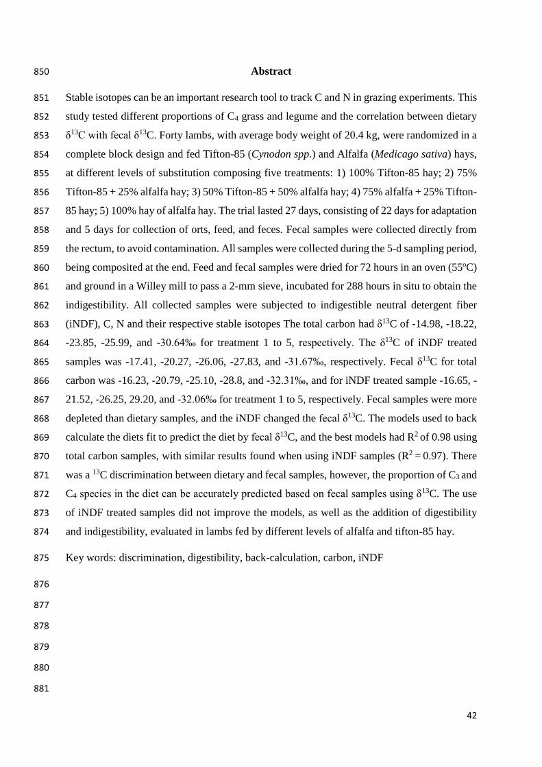
Abstract 850

Stable isotopes can be an important research tool to track C and N in grazing experiments. This 851

study tested different proportions of C4 grass and legume and the correlation between dietary 852

δ13C with fecal δ13C. Forty lambs, with average body weight of 20.4 kg, were randomized in a 853

complete block design and fed Tifton-85 (Cynodon spp.) and Alfalfa (Medicago sativa) hays, 854

at different levels of substitution composing five treatments: 1) 100% Tifton-85 hay; 2) 75% 855

Tifton-85 + 25% alfalfa hay; 3) 50% Tifton-85 + 50% alfalfa hay; 4) 75% alfalfa + 25% Tifton-856

85 hay; 5) 100% hay of alfalfa hay. The trial lasted 27 days, consisting of 22 days for adaptation 857

and 5 days for collection of orts, feed, and feces. Fecal samples were collected directly from 858

the rectum, to avoid contamination. All samples were collected during the 5-d sampling period, 859

being composited at the end. Feed and fecal samples were dried for 72 hours in an oven (55ºC) 860

and ground in a Willey mill to pass a 2-mm sieve, incubated for 288 hours in situ to obtain the 861

indigestibility. All collected samples were subjected to indigestible neutral detergent fiber 862

(iNDF), C, N and their respective stable isotopes The total carbon had δ13C of -14.98, -18.22, 863

-23.85, -25.99, and -30.64‰ for treatment 1 to 5, respectively. The δ13C of iNDF treated 864

samples was -17.41, -20.27, -26.06, -27.83, and -31.67‰, respectively. Fecal δ13C for total 865

carbon was -16.23, -20.79, -25.10, -28.8, and -32.31‰, and for iNDF treated sample -16.65, -866

21.52, -26.25, 29.20, and -32.06‰ for treatment 1 to 5, respectively. Fecal samples were more 867

depleted than dietary samples, and the iNDF changed the fecal δ13C. The models used to back 868

calculate the diets fit to predict the diet by fecal δ13C, and the best models had R2 of 0.98 using 869

total carbon samples, with similar results found when using iNDF samples (R2 = 0.97). There 870

was a 13C discrimination between dietary and fecal samples, however, the proportion of C3 and 871

C4 species in the diet can be accurately predicted based on fecal samples using δ13C. The use 872

of iNDF treated samples did not improve the models, as well as the addition of digestibility 873

and indigestibility, evaluated in lambs fed by different levels of alfalfa and tifton-85 hay. 874

Key words: discrimination, digestibility, back-calculation, carbon, iNDF 875

876

877

878

879

880

881

43

Introduction 882

883 884

Grass and legume mixtures provide environmental, ecological and productive 885

advantages. Legumes are not only a source of protein for livestock, but they also fix 886

atmospheric-N2, adding this element to grassland ecosystems (Dubeux et al. 2006). Nitrogen 887

is one of the main factors limiting livestock productivity. Therefore, the addition of N-fixing 888

legumes can increase primary productivity (Makkar, 2008). Including legumes to low quality 889

grass diet, increases the digestibility and intake, which improve animal response (Muir et al., 890

2011). One major challenge, however, is to obtain a representative sample of what the animal 891

is eating because of the animal selectivity. Moreover, a proxy for the real digestibility of the 892

selected diet is difficult to obtain, although in many cases in vitro digestibility has been used 893

(Carvalho et al., 2007). 894

When the pasture is a binary mixture of warm-season grass (C4) and legume (C3), these 895

plants have two different ways to fix carbon. The physiological mechanism inherent to these 896

distinct mechanism of fixation (C3 vs. C4), results in different levels of 13C discrimination. 897

Plants with C3 physiology have a range of δ13C from -26 to 32‰, and are more depleted in 13C 898

than plants with C4 physiology, which range from -9 to -17‰, due to the difference in 899

photosynthetic pathways (Ballentine et al., 1998; Fernandez et al., 2003). 900

Norman et al. (2009) reported that the natural abundance of stable isotopes and its 901

variability among photosynthetic pathways can be used to estimate the proportion of C3 and C4 902

plants in ruminant diets. Macedo et al. (2010) could estimate the proportions of grasses and 903

legumes in the diet of confined steers using fecal δ13C. Understanding diet composition of 904

ruminants will permit to assess the individual contribution of the grass and the legume 905

components on the animal performance. The relationship between fecal δ13C and the diet of 906

44

grazing animals is a way to assess it. Martins et al. (2012) reported that female sheep fed on a 907

C3 plant diet had different fecal samples than females fed on a C4 diet. 908

Possible differences in forage digestibility and feed interactions in ruminal conditions 909

could drive to wrong conclusions in a direct correlation of fecal δ13C with diet composition. 910

Feces and diet are often different in δ13C value. Some of the possible factors are endogenous 911

source of C, possible discrimination in the gut via microorganisms, and differences in 912

digestibility between the C3 and C4 species (Jones et al., 1979; Martins et al., 2012). The use 913

of neutral detergent fiber (NDF) analysis, which represent the fraction, that is unavailable for 914

microbial digestion in ruminant (Raffrenato et al., 2013), can be a useful tool to correct the 915

differences of δ13C from feces to diet. This process could eliminate endogenous and microbial 916

contamination present in the feces. 917

A feedlot trial in controlled conditions where intake and excreta are monitored is the best 918

option to validate models. These models could ultimately be applied to grazing animals, in 919

order to evaluate the proportions of C3 and C4 in animal diets. Thus, the objective of this 920

research was to assess the proportion of C3 and C4 forage species in the diet using iNDF δ13C, 921

based on fecal and dietary samples. We hypothesized that by analyzing the δ13C on the iNDF 922

we could estimate more accurately the proportion of the different species in the diet, reducing 923

contamination with endogenous carbon. 924

925

926

927

928

929

45

Material and Methods 930

931

Experimental site 932

The experiment was conducted at the Federal Rural University of Pernambuco (UFRPE), 933

in the small ruminant sector of the Animal Science Department located in Recife (8°01''S, 934

34°57'W,14 m asl), Pernambuco, Brazil. The temperature during the experimental period 935

varied between 22 and 31°C (APAC, 2017). 936

Animals and experimental diets 937

Experimental animals were forty lambs, Santa Ines mixed breed, with an average age of 938

3 months and body weight of 20.4 kg ± 1.8. Animals were arranged in a randomized complete 939

block design and placed in individual pens. The initial weight was used as a blocking criterion. 940

Before the beginning of the trial, anthelminthic was administered to all animals, and then they 941

were labeled, and randomly housed in pens within each block, with access to water and feeding 942

troughs. 943

Experimental diets (5) were replacement levels of Tifton-85 (Cynodon spp.) and Alfalfa 944

(Medicago sativa) hay: 1) 100% Tifton-85 hay; 2) 75% Tifton-85 + 25% alfalfa hay; 3) 50% 945

Tifton-85 + 50% alfalfa hay; 4) 75% alfalfa + 25% Tifton-85 hay; 5) 100% alfalfa hay. Diet 946

chemical composition is presented on Table 1. The alfalfa and Tifton-85 hay were obtained 947

from a local producer. The hay was ground in a forage grinder (Laboremus, Campina Grande, 948

PB, BR) to pass a 8-mm sieve with the objective of reducing the particle size in order to 949

improve the mixture of the material and avoid animal selectivity. Feed supply was adjusted to 950

3.4% of the body weight on a dry matter basis, reducing orts. Intake of the whole diet in each 951

meal was recorded. Water was offered ad libitum, being replaced every two days. Sheep were 952

fed twice daily, at 8:00 am and 3:00 pm. The experiment lasted 27 days, from December 11th 953

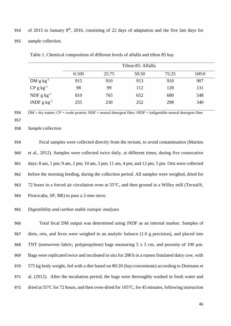
46

of 2015 to January 8th, 2016, consisting of 22 days of adaptation and the five last days for 954

sample collection. 955

Table 1. Chemical composition of different levels of alfalfa and tifton 85 hay

Tifton-85: Alfalfa

0:100 25:75 50:50 75:25 100:0

DM g kg-1 915 910 913 910 907

CP g kg-1 98 99 112 128 131

NDF g kg-1 810 765 652 680 548

iNDF g kg-1 255 230 252 298 340

DM = dry matter; CP = crude protein; NDF = neutral detergent fiber; iNDF = indigestible neutral detergent fiber 956

957

Sample collection 958

Fecal samples were collected directly from the rectum, to avoid contamination (Martins 959

et al., 2012). Samples were collected twice daily, at different times, during five consecutive 960

days: 8 am, 1 pm; 9 am, 2 pm; 10 am, 3 pm; 11 am, 4 pm; and 12 pm, 5 pm. Orts were collected 961

before the morning feeding, during the collection period. All samples were weighed, dried for 962

72 hours in a forced air circulation oven at 55°C, and then ground in a Willey mill (Tecnal®, 963

Piracicaba, SP, BR) to pass a 2-mm sieve. 964

Digestibility and carbon stable isotopic analyses 965

Total fecal DM output was determined using iNDF as an internal marker. Samples of 966

diets, orts, and feces were weighed in an analytic balance (1.0 g precision), and placed into 967

TNT (nonwoven fabric; polypropylene) bags measuring 5 x 5 cm, and porosity of 100 µm. 968

Bags were replicated twice and incubated in situ for 288 h in a rumen fistulated dairy cow, with 969

575 kg body weight, fed with a diet based on 80:20 (hay:concentrate) according to Detmann et 970

al. (2012). After the incubation period, the bags were thoroughly washed in fresh water and 971

dried at 55°C for 72 hours, and then oven-dried for 105°C, for 45 minutes, following instruction 972

47

of (Casali et al., 2008). The material incubated was submitted to NDF analysis (Detmann et al., 973

2012), and the iNDF samples were used to analyze the δ13C. 974

Feed intake was obtained by the difference between feed offered and orts. Diet DM 975

digestibility was determined using the difference between feed intake and fecal output, divided 976

by the feed intake (Azevedo et al., 2014): 977

𝐴) 𝐷𝑖𝑔𝑒𝑠𝑡𝑖𝑏𝑖𝑙𝑖𝑡𝑦 𝑜𝑓 𝐷𝑖𝑒𝑡 𝐷𝑀 =𝐼𝑛𝑡𝑎𝑘𝑒 − 𝑇𝑜𝑡𝑎𝑙 𝐹𝑒𝑐𝑎𝑙 𝑂𝑢𝑡𝑝𝑢𝑡

𝐼𝑛𝑡𝑎𝑘𝑒 978

Stable isotopic analyses were performed at the Forage Laboratory from the University of 979

Florida - North Florida Research and Education Center (NFREC), located in Marianna, Florida. 980

All samples and material remaining from the iNDF process were ball milled to reduce the 981

particle size under 100 µm, before the stable isotope analyses (Michener and Lajtha, 2007). 982

Samples were ball milled using a Mixer Mill MM400 (Retsch, Newton, PA, USA) at 25 Hz for 983

9 min. Samples were analyzed for total C and N using a CHNS analyzer through the Dumas 984

dry combustion method (Vario Micro Cube; Elementar, Hanau, GER) coupled to an isotope 985

ratio mass spectrometer (IsoPrime 100, IsoPrime, Manchester, UK) to analyze δ13C and δ15N. 986

The 13C/12C ratios are presented in the conventional delta (δ) notation, in per mil (‰) relative 987

to the Pee Dee Belemnite (PBD). Crude protein was estimated multiplying total N 988

concentration by 6.25. 989

Equation B, used to find the notation δ13C: 990

𝐵) 𝛿𝑀𝐸 = [(𝑅𝑆𝑎𝑚𝑝𝑙𝑒

𝑅𝑆𝑡𝑎𝑛𝑑𝑎𝑟𝑑⁄ ) − 1] ∗ 1000 991

Where E denotes the element, M is the mass of the heavy isotope, R is the ratio of the heavy to 992

light isotope for E, thus, the ratio of 13C:12C is expressed as δ13C (Ehleringer & Rundel, 1989; 993

Dawson & Brooks, 2001; Crawford et al., 2008). 994

48

Plant C sources from fecal samples were identified by the equation C, two-mixing pool, 995

(Fry, 2006): 996

𝐶) 𝑓1 =𝛿 𝑠𝑎𝑚𝑝𝑙𝑒 − 𝛿 𝑠𝑜𝑢𝑟𝑐𝑒 2

𝛿 𝑠𝑜𝑢𝑟𝑐𝑒1 − 𝛿 𝑠𝑜𝑢𝑟𝑐𝑒 2 997

𝑓1 + 𝑓2 = 1 (𝑜𝑟 𝑓1 = 1 − 𝑓2 ) 998

Where f 1 represents the fraction (contribuition) of source 1 e f 2 of source 2 999

The same equation above was used to determine the real proportion of C3 and C4 forage 1000

ingested by the sheep. The equation was applied to obtain the proportion (and amount) of each 1001

one of these diet components in the orts, for each individual animal, that were then subtracted 1002

from the supplied amount in order to find the real intake of each component. 1003

In order to estimate the proportion of each source in the diet, we also tested four models 1004

described by Norman et al. (2009) to back-calculate the diet. All the equations determined the 1005

proportion of C4 in the diet using fecal samples values. These equations were tested using δ13C 1006

determined on total C (sample without passing through the iNDF procedure) or in samples after 1007

passing through the iNDF procedure. The equation 1 is the same equation described above by 1008

Fry (2006) to mixed sources of C. 1009

1. %𝐶4 = 100 − {100 ∗ [(𝐴 − 𝐶)/(𝐵 − 𝐶)]} 1010

Where 1011

%C4 = Percentage of forage intake based on DM and in this case, a C4 grass 1012

A = δ13C of the animal feces 1013

B = δ13C of the C3 Plant 1014

C = δ13C of the C4 Plant 1015

1016

49

Eq. (2) is similar to eq. (1) but the discrimination between diet and feces was included. 1017

According to Norman et al. (2009), this equation assumes that diet-tissue discrimination rates 1018

are the same for both the C3 and C4 component of the diet. 1019

2. %C4 = 100 − {100 ∗ [(A − C − J)/(B − C)]} 1020

J = diet – feces discrimination* 1021

*Diet – Feces discrimination = δ13C of the animal feces - δ13C of the diet 1022

1023

This study used the discrimination as a constant number. The value used was the average 1024

of all discriminations, between all the treatments. The J value was -1.63‰ and it was obtained 1025

from the current dataset for this trial. 1026

Two different equations were used to assess the effect of in vivo indigestibility and 1027

digestibility. Norman et al. (2006) reported that for feces, the back calculation should correct 1028

for relative indigestibility (eq. 3a), and the samples as blood or wool should be corrected with 1029

relative digestibility. This study just used feces to back calculate the diet, then eq. 4 will 1030

represent only samples of feces. 1031

3a. %𝐶4 = 100 − 100/({[𝐹 ∗ ((𝐵 + 𝐽) − 𝐴)]/[𝐺 ∗ (𝐴 − (𝐶 + 𝐽))) ]} + 1) 1032

3b. %𝐶4 = 100 − 100/({[𝐷 ∗ ((𝐵 + 𝐽) − 𝐴)]/[𝐸 ∗ (𝐴 − (𝐶 + 𝐽))) ]} + 1) 1033

Where 1034

D = % Dry matter in vivo digestibility of C3 plants 1035

E = % Dry matter in vivo digestibility of C4 plants 1036

F = 100 - % Dry matter in vivo digestibility of C3 plants 1037

G = 100 - % Dry matter in vivo digestibility of C4 plants 1038

1039

Eq. (4) uses the δ13C of the animal feces and the δ13C of feces collected from animals that ate 1040

exclusively plants of C3 or C4, in order to back calculate the proportion in the diet. 1041

1042

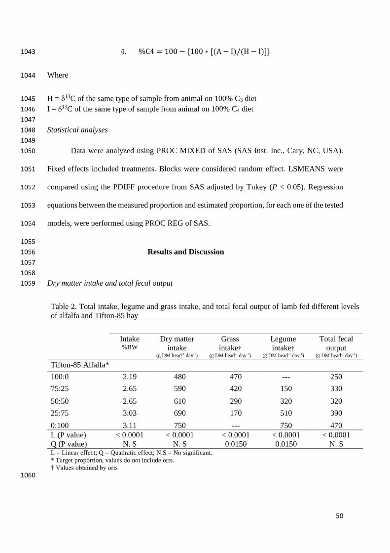
50

4. %C4 = 100 − {100 ∗ [(A − I)/(H − I)]} 1043

Where 1044

H = δ13C of the same type of sample from animal on 100% C3 diet 1045

I = δ13C of the same type of sample from animal on 100% C4 diet 1046

1047

Statistical analyses 1048

1049

Data were analyzed using PROC MIXED of SAS (SAS Inst. Inc., Cary, NC, USA). 1050

Fixed effects included treatments. Blocks were considered random effect. LSMEANS were 1051

compared using the PDIFF procedure from SAS adjusted by Tukey (P < 0.05). Regression 1052

equations between the measured proportion and estimated proportion, for each one of the tested 1053

models, were performed using PROC REG of SAS. 1054

1055

Results and Discussion 1056

1057

1058

Dry matter intake and total fecal output 1059

Table 2. Total intake, legume and grass intake, and total fecal output of lamb fed different levels

of alfalfa and Tifton-85 hay

Intake %BW

Dry matter

intake (g DM head-1 day-1)

Grass

intake† (g DM head-1 day-1)

Legume

intake† (g DM head-1 day-1)

Total fecal

output (g DM head-1 day-1)

Tifton-85:Alfalfa*

100:0 2.19 480 470 --- 250

75:25 2.65 590 420 150 330

50:50 2.65 610 290 320 320

25:75 3.03 690 170 510 390

0:100 3.11 750 --- 750 470

L (P value) < 0.0001 < 0.0001 < 0.0001 < 0.0001 < 0.0001

Q (P value) N. S N. S 0.0150 0.0150 N. S L = Linear effect; Q = Quadratic effect; N.S = No significant.

* Target proportion, values do not include orts.

† Values obtained by orts 1060

51

There was a linear increase (P<0.0001) in dry matter intake (DMI) and in the intake as 1061

a percentage of body weight (BW) with increasing levels of alfalfa hay in the diet (Table 2). 1062

Grass DMI on 100% grass diet was 470 g DM hd-1 d-1, while the pure legume DMI was 750 g 1063

DM hd-1 d-1. There was a quadratic effect (P= 0.0150) for legume and grass intake. The 1064

obtained intake increment due to the replacement of grass by legume was expected and it was 1065

equivalent to that reported by Burns and Fisher (2013) replacing the diet of steers from mature 1066

grass to alfalfa, at different levels. In this present study, Tifton-85 hay had greater NDF 1067

concentration (Table 1). Thus, the replacement of grass by legume decreased the NDF 1068

concentration in the diet, increasing DMI as a result. Van Soest (1994) reported that low forage 1069

quality and high fiber concentration in the diet limit forage intake. However, chemical 1070

degradation and physical breakdown in the rumen directly influence legume intake in relation 1071

to grass, because of the rumen filling effect (Dewhurst et al., 2009). Low-energy and high-1072

filling diets depress intake by a physical mechanism. Thereby, NDF is considered a feed 1073

characteristic that is directly related to the filling effect of the diet (Mertens, 2007). NDF 1074

digestibility also plays a role, considering that different compounds such as lignin, cellulose, 1075

and hemicellulose can make up different proportions of the NDF, depending on the forage 1076

species, environmental conditions, and maturity of the plant (Van Soest, 1994). 1077

Alfalfa hay DMI in the pure diet was similar to the intake values (67 to 74 g kg d-1 1078

BW0.75) observed by Wildeus et al. (2007) for three breeds of wool sheep. This result is also 1079

consistent with Park et al. (1989) who found greater DMI for alfalfa than for bermudagrass 1080

(coastal), 61.3 g kg d-1 BW0.75 and 57.8 g kg d-1 BW0.75 respectively. In addition to the 1081

preference for alfalfa hay, grass fiber concentration might have contributed to the reduced 1082

intake. In this study, Tifton-85 hay NDF concentration (810 g kg-1) was greater than the NDF 1083

concentration found by Lopes (2015; 756.1 g kg-1 DM) and Coelho (2015; 703 g kg DM) for 1084

the same grass. Increase of intake after inclusion of alfalfa in the diet is also supported by 1085

52

Manaye et al. (2009), who observed an increase of DMI from 57.9 g kg BW-0.75 to 63.1 g kg 1086

BW-0.75 after the supplementation of legume in the grass-based diet of sheep. 1087

Grass NDF in that study (715 g kg-1 DM) was greater than legume NDF (399 g kg-1 1088

DM). Tamir and Asefa (2009) studied the effect of legume inclusion (Acacia saligna) on the 1089

voluntary feed intake of lambs on a diet based on grass hay. Legume inclusion improved total 1090

DMI of lambs. Przemysław et al. (2015) reported greater DMI of alfalfa (cv. Alba) silage, than 1091

red clover (cv. Nike), and red fescue (cv. Godolin) silage to lambs. The NDF concentrations of 1092

red clover and fescue were 509 and 590 g kg-1 DM, respectively, greater than the NDF 1093

concentration of alfalfa silage, which was 462 g kg-1 DM, resulting in a lower DMI. Bamikole 1094

et al. (2001) observed a different result when feeding goat with grass–legume mixture, and 1095

fertilized and unfertilized grass. The DMI was considered similar among these diets (208, 244, 1096

and 220 g kg-1 DM d-1, respectively) with equivalent NDF concentration. 1097

Particle size is another factor that might have contributed to increase forage intake. 1098

Smaller feed particles increase passage rate and feed intake, but reduces digestibility. Van Soest 1099

(1994) indicated that the reduction of particle size before feeding, by grinding, can increase 1100

forage intake. Smaller feed particles increase diet density, which leads to faster passage rates 1101

and less rumen volume, reducing rumination time as a result. Particle size reduction is crucial 1102

for disruption of the cuticle and cell wall membranes, exposing cell contents and enhancing 1103

access for microbes and enzymes (Mertens, 2007). Legumes, in general, have less NDF 1104

concentration than warm-season grasses, being more easily degradable by rumen 1105

microorganism. 1106

The alfalfa and Tifton-85 hay used in this study were ground to improve intake, reduce 1107

selectivity, and minimize orts. The amount of forage offered was limited to 3% of the BW; 1108

limiting the intake and reducing the selectivity of plant parts, as well as of forage species. The 1109

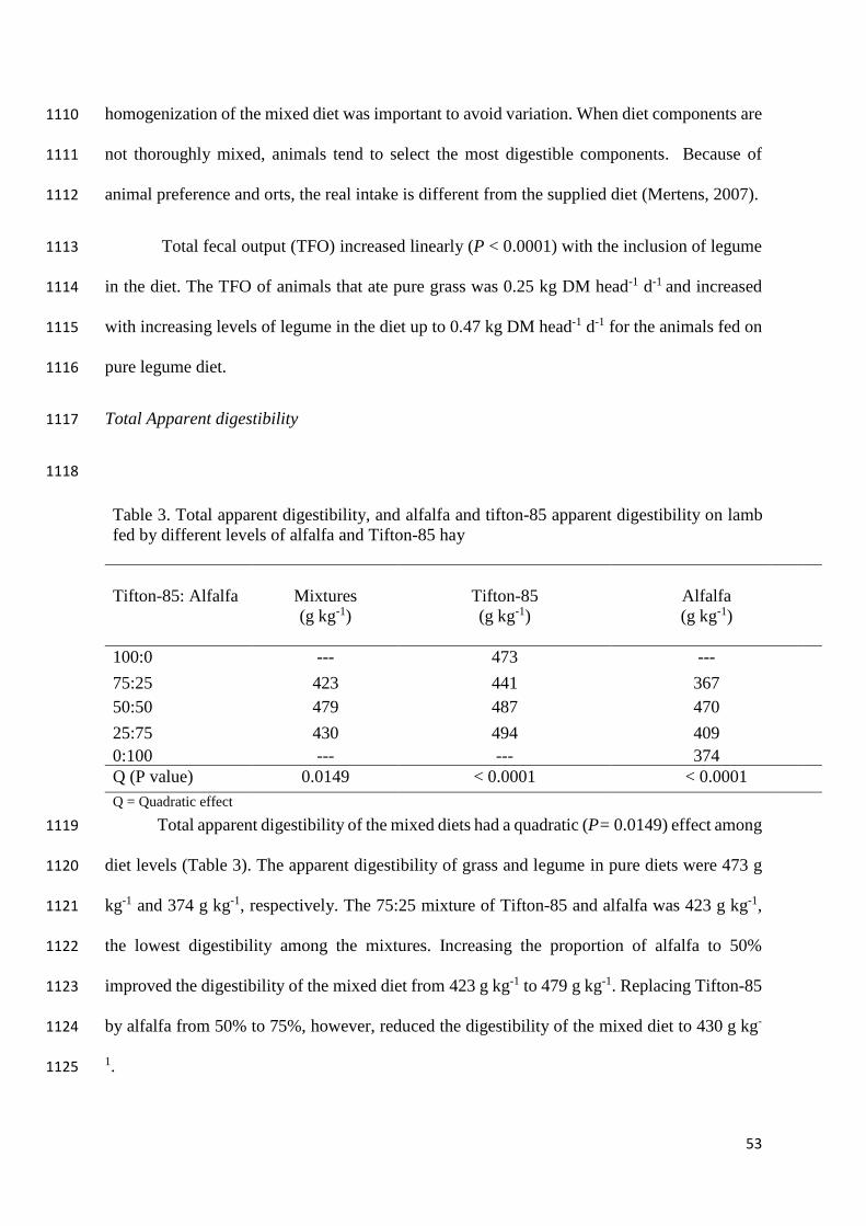
53

homogenization of the mixed diet was important to avoid variation. When diet components are 1110

not thoroughly mixed, animals tend to select the most digestible components. Because of 1111

animal preference and orts, the real intake is different from the supplied diet (Mertens, 2007). 1112

Total fecal output (TFO) increased linearly (P < 0.0001) with the inclusion of legume 1113

in the diet. The TFO of animals that ate pure grass was 0.25 kg DM head-1 d-1 and increased 1114

with increasing levels of legume in the diet up to 0.47 kg DM head-1 d-1 for the animals fed on 1115

pure legume diet. 1116

Total Apparent digestibility 1117

1118

Total apparent digestibility of the mixed diets had a quadratic (P= 0.0149) effect among 1119

diet levels (Table 3). The apparent digestibility of grass and legume in pure diets were 473 g 1120

kg-1 and 374 g kg-1, respectively. The 75:25 mixture of Tifton-85 and alfalfa was 423 g kg-1, 1121

the lowest digestibility among the mixtures. Increasing the proportion of alfalfa to 50% 1122

improved the digestibility of the mixed diet from 423 g kg-1 to 479 g kg-1. Replacing Tifton-85 1123

by alfalfa from 50% to 75%, however, reduced the digestibility of the mixed diet to 430 g kg-1124

1. 1125

Table 3. Total apparent digestibility, and alfalfa and tifton-85 apparent digestibility on lamb

fed by different levels of alfalfa and Tifton-85 hay

Tifton-85: Alfalfa

Mixtures

(g kg-1)

Tifton-85

(g kg-1)

Alfalfa

(g kg-1)

100:0 --- 473 ---

75:25 423 441 367

50:50 479 487 470

25:75 430 494 409

0:100 --- --- 374

Q (P value) 0.0149 < 0.0001 < 0.0001

Q = Quadratic effect

54

There was a quadratic effect (P <0.0001) for the digestibility of the individual 1126

components in the mixed diets, varying with their participation in each mixed diet. The mixture 1127

of Tifton-85 and alfalfa up to 50% improved both digestibilities. Alfalfa digestibility increased 1128

from 374 to 470 g kg-1, and Tifton-85 from 473 to 487 g kg-1, for 100% to 50% inclusion, 1129

respectively. Increasing levels of alfalfa improved Tifton-85 digestibility. 1130

Alfalfa digestibility was untypically low, and differed from literature values. Parker et 1131

al. (1989) observed alfalfa digestibility of 673 g kg-1, Wildeus et al. (2007) reported alfalfa 1132

digestibility ranging from 583 to 630 g kg-1, and Burns and Fisher (2013) as 788 g kg-1. This 1133

unusual result was probably due to the reduced particle size of the alfalfa hay, maturity stage, 1134

and iNDF concentration. The same hay was incubated (in situ) in a ruminal fistulated cow and 1135

the digestibility was 570 g kg-1 DM (Table 3). This value is similar to that obtained by Nelson 1136

and Satter (1992), who found 560 g kg-1 DM in late cut alfalfa hay and greater than 516 g kg-1 1137

DM of alfalfa at early flower maturity stage after 36 hours of incubation, obtained by Yari et 1138

al. (2012). Alfalfa digestibility from the in vivo trial, however, is lower than the one obtained 1139

from the in situ digestibility trial. The time of 48 h used to determine the digestibility in situ, 1140

could, contribute to this value, due to the opportunity to degrade. Furthermore, the passage rate 1141

was not an issue in this case, as observed in the in vivo trial. 1142

The mature alfalfa studied by Yari et al. (2012) had CP of 162 g kg-1 DM and NDF of 1143

491 g kg-1 DM, values different than the ones obtained in this study, i.e. 131 g kg-1 DM for CP 1144

and 548 g kg-1 DM and NDF (Table 1). The alfalfa used in this study was poor in protein and 1145

high in fiber, reasons that can be related to its low digestibility. Lacefield et al. (2009) reported 1146

values for alfalfa CP ranging from 90 to 130 g kg-1 DM and NDF from 560 to 600 g kg-1 DM 1147

at late bloom maturity stage. These values are similar to the ones obtained in this study. 1148

Palmonari et al. (2014) reported that alfalfa maturity influences its CP and fiber, affecting 1149

significantly the digestibility. Later maturity is responsible for greater fiber and lignin 1150

55

concentrations and reduced CP, digestibility and alfalfa hay quality (Lacefield et al., 2009; Yari 1151

et al. 2014). 1152

The alfalfa and Tifton-85 hay were ground in a forage grinder to facilitate the 1153

homogenization of the mixtures. The sieve used to grind was 8 mm, which possibly reduced 1154

the particle size down to a point that affected passage rate and digestibility (Mertens, 2007). 1155

Van Soest (1994) can also explain the low digestibility observed for the alfalfa used in this 1156

study. Finer feed particle degrades faster due to increased surface area. Reduced time for 1157

ruminal degradation, however, results in less rumination, because of the particle size density, 1158

resulting in lower digestibility. The grinding effect can be compared to rumination in terms of 1159

digestive effect (Minson, 1990). For sheep, the consequence of hay small particles is the 1160

reduction of the time in the tract, reducing the digestibility of the organic matter and fiber. 1161

The iNDF concentration represents the indigestible fraction of the forage and can be 1162

considered another factor responsible to reduce digestibility. The alfalfa hay used in this study 1163

had 330 g kg -1 DM of iNDF (Table 1) and differed from the iNDF of mature alfalfa analyzed 1164

by Palmonari et al. (2014) in a two-year study, that was 167 g kg -1 DM and 175 g kg -1 DM. 1165

Dietary and fecal δ13C based on total C and iNDF samples 1166

As expected, increasing levels of alfalfa resulted in more depleted samples in 13C, both 1167

for fecal and dietary samples (Table 4). All fecal samples were more depleted than diet samples, 1168

except the iNDF-treated samples in which 50% of each component was supplied. Average 1169

discrimination between feces and diet was greater for untreated samples than for iNDF-treated 1170

samples. 1171

1172

1173

56

Table 4. Dietary and fecal δ13C, and discrimination based on total sample C and indigestible neutral

fiber treated samples

Tifton-85: Alfalfa

Diet (‰)

Feces (‰)

Δδ

P value

Total C samples

100:0 -14.98 -16.23 -1.25 <0.0001

75:25 -18.22 -20.79 -2.57 <0.0001

50:50 -23.85 -25.10 -1.25 0.00091

25:75 -25.99 -28.78 -2.75 <0.0001

0:100 -30.64 -32.31 -1.67 <0.0001

iNDF treated samples

100:0 -17.41 -16.56 0.85 <0.0001

75:25 -20.27 -21.52 -1.25 <0.0001

50:50 -26.09 -26.25 -0.17 0.40480

25:75 -27.83 -29.20 -1.37 0.00071

0:100 -31.67 -32.06 -0.39 0.00332

P value = T Student (p>0.05) comparing δ13C between diet and feces samples; Δδ = difference between feces and

diet

Grass diet δ13C was -14.98‰ and fecal δ13C was -16.23‰, with a discrimination of – 1174

1.25‰, while legume diet δ13C was -30.64‰ and fecal δ13C was -32.31‰, with a 1175

discrimination of -1.67‰. The δ13C assessed from feces in this present study was more depleted 1176

than the diet δ13C. The result obtained in the pure legume diet differ with the reported by 1177

Sponheimer et al. (2003), Macedo et al. (2010), and Martins et al. (2012), where they did not 1178

identify δ13C difference between feces and legume diet. The discrimination between diet and 1179

feces, in total carbon samples observed in this study, were in the same range observed by Jones 1180

et al. (1979); Sponheimer et al. (2003); Hwang et al. (2007); Norman et al. (2009); and Macedo 1181

et al. (2010). 1182

Diet and fecal δ13C assessed on iNDF-treated samples indicated that these samples 1183

became more depleted after iNDF analysis. Pure diets and feces had δ13C of -17.41 and -1184

16.56‰ (P>0.0001) for grass and -31.67‰ and -32.06‰ (P=0.00322) for legume, 1185

respectively. The Δδ for grass and legume were 0.85 and -0.39‰, respectively. For mixed diets, 1186

57

the δ13C value became depleted when legumes were included in the mixture, as observed with 1187

samples based on total carbon. In the diet with 25% of legume inclusion, the δ13C was -20.27‰ 1188

and the feces, -21.52‰ (P<0.0001). When the amounts of legume and grass were the same 1189

(50:50), the δ13C value of the diet was -26.09‰ and the feces -26.25‰ and the Δδ of – 0.17 ‰ 1190

was not significantly different (P=0.4048). The δ13C values of diet and feces, with 75% of 1191

legume inclusion, were -27.83‰ and -29.20‰ (P=0.0070), respectively, with a Δδ value of -1192

1.37‰. 1193

The δ13C results for alfalfa and Tifton-85 were within the range of C3 and C4 plants 1194

(Ballentine et al.,1998), alfalfa being more depleted than the one used by Sponheimer et al. 1195

(2003), which was -27.0‰. Martins et al. (2012) found δ13C -31.15‰ in alfalfa hay, with NDF 1196

concentration of 574.5 g kg -1 DM, values similar to the ones found in this study (NDF = 548 1197

g kg -1 DM). Alfalfa hay δ13C in the present study was more depleted, perhaps, due to greater 1198

NDF concentration, because of the maturity stage of the plant. Leaf and stem ratio can influence 1199

the fractionation of δ13C in the bulk analysis. Leaves are more enriched in δ13C than stems and 1200

roots (O`Leary, 1988). Stems function as plant support and are rich in fiber and lignin (Taiz 1201

and Zeiger, 2002), differently from leaves, that are responsible for photosynthesis. Fernandez 1202

et al. (2003) reported that the δ13C value of lignin, cellulose, and the bulk of Lolium perene, 1203

were -30.3‰, -26.50‰, and -28.5‰, respectively. Greater proportion of stem, with greater 1204

fiber and lignin levels, can lead to more negative δ13C values. 1205

In addition, the temperature of the region where these plants grew possibly pushed 1206

down the δ13C value. O`Leary (1988) reported that environmental effects on δ13C value in C3 1207

plants can occur due to the increase in temperature, which can move the signal to 3‰, negative. 1208

Thus, the signal of plants of the same species, and the same metabolism, can vary (Farquhar et 1209

al.,1982). 1210

58

Tifton-85 hay δ13C was compatible with the ones observed for C4 plants. The value 1211

found by the present study was similar to the ones observed by Sponheimer et al. (2003), who 1212

reported -14.1‰ for bermudagrass (Cynodon dactylon) and by Norman et al. (2009) that found 1213

-14.9‰, for saltbush (Atriplex nummularia Lindl.). 1214

The δ13C value of grass and legume, from iNDF-treated samples,were also similar to 1215

the ones reported for the C3 and C4 plants (Ballentine et al.,1998). The δ13C on treated samples, 1216

however, changed after the incubation, certainly, due to ruminal degradation and NDF analysis. 1217

The δ13C of diets that were submited to the iNDF process became more depleted, and the feces 1218

stayed in the same pattern than the total carbon samples. However, the grass diet had a different 1219

discrimination, feces becaming more positive than diet, a situation different from the rest of 1220

the diets. The diet became more negative than the diets before incubation, as the rest of the 1221

diets. Probably, this discrimination came from the effect of the incubation plus the NDF 1222

solution, in this grass. Samples from this diet were degraded by microorganisms from rumen 1223

during 288 h, and were washed in neutral detergent thereafter, which removed some parts of 1224

the fiber; the same happened in the incubation. The signal obtained was different than those 1225

obtained in the feces, so the negative signature indicates greater proportion of indigestible 1226

fibers in this sample. The diet with 50% of grass and 50% of legume, after iNDF treatment, 1227

had the same signal as the feces. 1228

The feces after iNDF process became -0.85‰, more negative than feces based on total 1229

carbon. This likely occurred because NDF incubation and NDF solution might have changed 1230

the signal of the diet, becoming similar to the ones observed in the feces. Discrimination 1231

between feces and diet is sometimes reported in the literature as an influence of endogenous 1232

contamination of the feces from gut tissue, microorganisms and other sources of carbon (Jones 1233

et al., 1979; Norman et al., 2009; Martins et al., 2012). This is not clear in the results presented 1234

in this study, since the NDF solution changed the signal of the diet, which became more 1235

59

negative, but did not affect the fecal δ13C. The contaminations present in the feces must have 1236

been removed after the NDF process, altering the δ13C. Sponheimer et al. (2003) observed that 1237

after treating samples using the ADF process, the fecal δ13C did not change. They related that 1238

the contamination by microorganism could not be the factor that turn the fecal δ13C negative, 1239

because the effect of ADF solution, that can remove it. 1240

One possible reason for this discrimination between diet and feces is the degradation of 1241

the plant material by rumen microorganisms. Fractionation of plant components is different, 1242

varying the δ13C of protein, carbohydrate, lipids, fiber, and lignin (Ballentaine et al 1998; 1243

Fernandez et al. 2003). The action of microbes over the vegetal tissue removes components 1244

from the feces, that have different δ13C, and they may be depleted or enriched. The iNDF 1245

process showed that samples incubated in the bags for 12 days will represent the indigestible 1246

fraction, fiber that was not degraded by the bacteria, and has a different δ13C free of 1247

contamination. Sponheimer et al. (2003) demonstrated that alfalfa has the same bulk and ADF 1248

signature, -27.0 and -27.1‰ respectively, and bermudagrass a bulk more negative than ADF, 1249

-14.1 and -12.7‰. Fernandez et al. (2003) reported that lignin of corn is depleted in 13C, 1250

compared to cellulose, and bulk material. 1251

The iNDF process did not reduce the discrimination between diet and feces. The iNDF 1252

changed the signature of diets, and had no effect in feces. Lignin was more depleted than the 1253

whole plant. The material that remained after the iNDF procedure is mostly represented, by 1254

lignin, and cellulose. In mixed diets, the lignin of legume and grass are different in δ13C, thus, 1255

in feces, the signal is going to be the δ13C of lignin and cellulose, and cannot be reversed, by 1256

iNDF of feces, used to correct the fecal signal. 1257

1258

1259

60

Models used to back calculate the animal diet 1260

All models used to predict the proportion of C4 plants in the diet, total carbon and iNDF 1261

residue, fitted to predicted values (P < 0.0001). Equations 1, 2, and 4 had the same adjusted 1262

R2, coefficient of variation, and root mean square error in total carbon samples and iNDF-1263

treated samples. Equations 3a and 3b had the lowest adjusted R2 among all equations in the 1264

total carbon analysis, as well as the greater CV and RMSE (Table 5). For iNDF-treated samples, 1265

the pattern was similar, with equation 3a having the lowest RMSE and CV and the greatest 1266

adjusted R2 (Table 5). The models that used the total carbon to predict the C4 proportions are 1267

presented in the Figure 1, and the models that used iNDF residue are presented in the Figure 2. 1268

Table 5. Models using total sample carbon and indigestible neutral fiber δ13C to trace back

the diet of ruminants

Total C samples

Models Adjusted R2 CV (%) RMSE

1 0.986 8.5 4.2

2 0.986 8.5 4.2

3a 0.978 11.0 5.3

3b 0.975 11.9 5.8

4 0.986 8.5 4.2

iNDF-treated samples

1 0.973 11.7 5.8

2 0.973 11.7 5.8

3a 0.979 10.7 5.2

3b 0.954 16.1 7.8

4 0.974 11.7 5.8 CV = coefficient of variation; RMSE = Root mean square error

Eq 1: %C4=100- {100*[(δ13C feces - δ13C; C4 plants)/ (δ13C; C3 plants - δ13C; C4 plants)]}

Eq 2: %C4=100- {100*[(δ13C feces - δ13C; C4 plants-Δδ)/ (δ13C; C3 plants - δ13C; C4 plants)]}

Eq 3a: %C4=100-100/ ({[Indigestibility C3*((δ13C; C3 plants + Δδ)- δ13C feces)]/

[ Indigestibility C4*(δ13C feces -( δ13C; C4 plants +Δδ)))]} +1)

Eq 3b: %C4=100-100/ ({[ Digestibility C3*((δ13C; C3 plants + Δδ)- δ13C feces)]/

[ Digestibility C4*(δ13C feces -( δ13C; C4 plants +Δδ)))]} +1)

Eq 4: %C4=100- {100*[(δ13C feces - δ13C feces; C3)/ (δ13C feces; C4- δ13C feces; C3)]}

1269

1270

61

1271

1272

1273

1274

1275

1276

1277

1278

1279

1280

y = 0.9551x + 12.121

R² = 0.9865

-20

0

20

40

60

80

100

120

-20 5 30 55 80 105

Pre

dic

ted

C4 (

%)

1

P< 0.0001

y = 0,8995x + 7,9889

R² = 0,9801

-20

0

20

40

60

80

100

120

-20 5 30 55 80 105

Pre

dic

ted

C4

(%)

3a

P< 0.0001

y = 0,9619x + 3,5976

R² = 0,9753

-20

0

20

40

60

80

100

120

-20 5 30 55 80 105

Pre

dic

ted

C4

(%)

Observed C4 (%)

3b

P< 0.0001

y = 0,9551x + 2,1793

R² = 0,9865

-20

0

20

40

60

80

100

120

-20 5 30 55 80 105

Pre

dic

ted

C4

(%)

2

P< 0.0001

y = 0.9801x + 1.9963

R² = 0.9865

-20

0

20

40

60

80

100

120

-20 5 30 55 80 105

Pre

dic

ted

C

4(%

)

4

P< 0.0001

Figure 1. Proportion of C4 plant in the diet predicted by models, using total carbon values. 1= % C4 vs equation 1; 2 =

% C4 vs equation 2; 3a = % C4 vs equation 3a; 3b = % C4 vs equation 3b; 4 = % C4 vs equation 4.

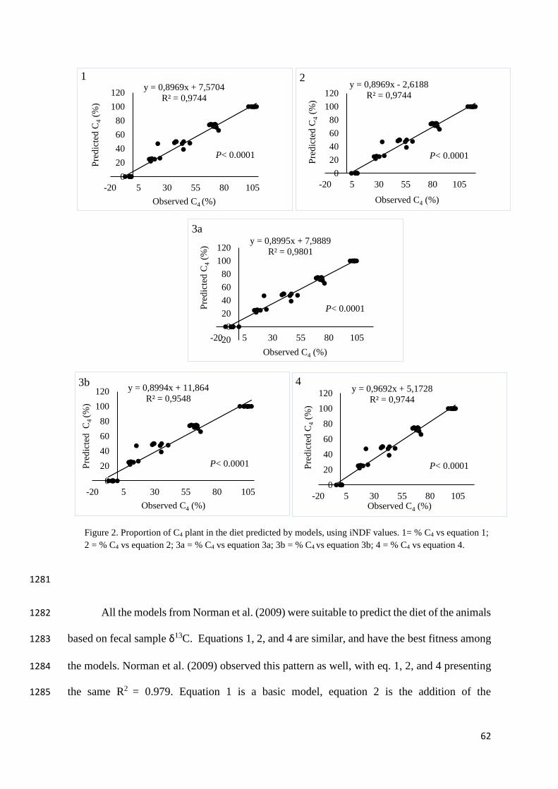
62

1281

All the models from Norman et al. (2009) were suitable to predict the diet of the animals 1282

based on fecal sample δ13C. Equations 1, 2, and 4 are similar, and have the best fitness among 1283

the models. Norman et al. (2009) observed this pattern as well, with eq. 1, 2, and 4 presenting 1284

the same R2 = 0.979. Equation 1 is a basic model, equation 2 is the addition of the 1285

y = 0,8969x + 7,5704

R² = 0,9744

0

20

40

60

80

100

120

-20 5 30 55 80 105

Pre

dic

ted

C4

(%)

Observed C4 (%)

1y = 0,8969x - 2,6188

R² = 0,9744

0

20

40

60

80

100

120

-20 5 30 55 80 105

Pre

dic

ted

C4

(%)

Observed C4 (%)

2

y = 0,8995x + 7,9889

R² = 0,9801

-20

0

20

40

60

80

100

120

-20 5 30 55 80 105

Pre

dic

ted

C4

(%)

Observed C4 (%)

3a

y = 0,8994x + 11,864

R² = 0,9548

0

20

40

60

80

100

120

-20 5 30 55 80 105

Pre

dic

ted

C

4 (

%)

Observed C4 (%)

3by = 0,9692x + 5,1728

R² = 0,9744

0

20

40

60

80

100

120

-20 5 30 55 80 105

Pre

dic

ted

C4

(%)

Observed C4 (%)

4

Figure 2. Proportion of C4 plant in the diet predicted by models, using iNDF values. 1= % C4 vs equation 1;

2 = % C4 vs equation 2; 3a = % C4 vs equation 3a; 3b = % C4 vs equation 3b; 4 = % C4 vs equation 4.

P< 0.0001

P< 0.0001

P< 0.0001

P< 0.0001

P< 0.0001

63

discrimination, and the equation 4 requires the separate discrimination of C3 and C4 plant in 1286

diet and feces. These equations are related with the addition of a constant number, therefore, 1287

the data are similar. Equation 3a and 3b are similar to equation 2, but with addition of 1288

indigestibility or digestibility and the addition of this component increased the error. The 1289

addition of the indigestibility did not improve the accuracy, differently from the data obtained 1290

by Norman et al. (2009), which the R2 was 0.994. In general, the methods to predict are suitable, 1291

but, for grazing conditions, equation 1 is more practical because it has less components than 1292

the other equations. 1293

Our hypothesis that the iNDF residue can improve the accuracy of the diet prediction, 1294

is not supported by these results. The results presented can clarify that, the use of δ13C from 1295

iNDF components did not increase the prediction. The iNDF process changed the δ13C of the 1296

diet. These results confirm these obtained by Jones et al. (1979), when they used fecal NDF in 1297

sheep feces and did not improve the relationship between diet and feces. 1298

Conclusion 1299

There is a 13C discrimination between dietary and fecal samples. However, the 1300

proportion of C3 and C4 species in the diet can be accurately predicted based on fecal samples 1301

using δ13C. The addition of digestibility and indigestibility did not improve the models in this 1302

study. The use of iNDF did not improve the prediction compared with the total sample. All the 1303

models fitted to predict, however, the equation 4 has one factor that can reduce its use, which 1304

is the inclusion of δ13C from feces of animals on exclusive C3 plants diet. Equation 1 is 1305

recommended to back calculate the proportion of C3 and C4 plants in diets of lambs based on 1306

fecal δ13C because of its simplicity and accuracy. 1307

1308

1309

64

References 1310

1311

APAC, Agencia pernambucana de aguas e clima, 2017. 1312 http://www.apac.pe.gov.br/meteorologia/boletins_climaticos_old.php. (accessed 3.23.17) 1313

Azevedo, E.B., Poli, C.H.E.C., David, D.B., Amaral, G.A., Fonseca, L., Carvalho, P.C.F., 1314 Fischer, V., Morris, S.T., 2014. Use of faecal components as markers to estimate intake 1315 and digestibility of grazing sheep. Livest. Sci. 165, 42–50. 1316

Ballentine, D.C., Macko, S.A., Turekian, V.C., 1998. Variability of stable carbon isotopic 1317 compositions in individual fatty acids from combustion of C 4 and C 3 plants: 1318 implications for biomass burning. Chem. Geol. 151–161. 1319

Bamikole, M.A., Ezenwa, I., Akinsoyinu, A.O., Arigbede, M.O., Babayemi, O.J., 2001. 1320 Performance of West African dwarf goats fed Guinea grass - Verano stylo mixture, N-1321

fertilized and unfertilized Guinea grass. Small Rumin. Res. 39, 145–152. 1322

Burns, J.C., Fisher, D.S., 2013. Steer responses to increasing proportions of legume when fed 1323 switchgrass hay Cooperative investigation of the USDA-ARS and the North Carolina 1324 ARS, Raleigh 27695-7642. Prof. Anim. Sci. 29, 383–394. 1325

Carvalho, P.C. de F., Kozloski, G.V., Filho, H.M.N.R., Reffatti, M.V., Genro, T.C.M., 1326 Euclides, V.P.B., 2007. Advances in methods for determining animal intake on pasture. 1327

Rev. Bras. Zootec. 36, 151–170. 1328

Casali, A.O., Detmann, E., Valadares Filho, S.D.C., Pereira, J.C., Henriques, L.T., De 1329 Freitas, S.G., Paulino, M.F., 2008. Influência do tempo de incubação e do tamanho de 1330

partículas sobre os teores de compostos indigestíveis em alimentos e fezes bovinas 1331 obtidos por procedimentos in situ. Rev. Bras. Zootec. 37, 335–342. 1332

Crawford, K., Mcdonald, R., Bearhop, S., 2008. Applications of stable techiques to the 1333

ecology of mammals. Mammal Rev. 38, 87–107. 1334

Dawson, T.E., Brooks, P.D., 2001. Fundamentals of stable isotope chemistry and 1335 measurement, in: Stable Isotope Techniques in the Study of Biological Processes and 1336

Functioning of Ecosystems. pp. 1-18. 1337

Detmann, E.; Souza, M.A.; Valadares Filho, S.C.; Queiroz, A.C.; Berchielli, T.T.; Saliba, 1338

E.O.S.; Cabral, L.S.; Pina, D.S.; Ladeira, M.M.; Azevedo, J.A.G., 2012. Métodos para 1339 análise de alimentos. Visconde do Rio Branco: Suprema pp, 214. 1340

Dewhurst, R.J., Delaby, L., Moloney, A., Boland, T., Lewis, E., 2009. Nutritive value of 1341 forage legumes used for grazing and silage. Irish J. Agric. Food Res. 48, 167–187. 1342

Dubeux Jr, J.C.B.; Lira, M.A.; Santos, M.V.F.; Cunha, M. D. Fluxo de nutrientes em 1343

ecossistemas de pastagens: impactos no ambiente e na produtividade, in: Simpósio sobre 1344 o Manejo da Pastagem, 23., Piracicaba. 2006. Anais ... Piracicaba: FEALQ, 2006, p.439-1345 506. 1346

Ehleringer, J.R., Rundel, P.W., 1989. Stable isotopes: History, units, and instrumentation, in: 1347 stable isotopes in ecological research (ecological studies 68). pp. 1–16. 1348

Farquhar, G., O’Leary, M., Berry, J., 1982. On the relationship between carbon isotope 1349 discrimination and the intercellular carbon dioxide concentration in leaves. Aust. J. Plant 1350 Physiol. 9, 121. 1351

65

Fernandez, I., Mahieu, N., Cadisch, G., 2003. Carbon isotopic fractionation during 1352

decomposition of plant materials of different quality. Global Biogeochem. Cycles 17, 1353

Hwang, Y.T., Millar, J.S., Longstaffe, F.J., 2007. Do δ 15 N and δ 13 C values of feces 1354 reflect the isotopic composition of diets in small mammals? Can. J. Zool. 85, 388–396. 1355

Jones, R.J., Ludlow, M.M., Troughton, J.H., G, B.C., 1979. Estimating eaten C3 and C4 from 1356 feaces. J. Agric. Sci. 91–100. 1357

Lacefield, G.D., D.M. Ball, D. Hancock, J. Andrae, And R. Smith. 2009. Growing alfalfa in 1358 the South. National alfalfa and forage alliance. 1359 https://www.alfalfa.org/pdf/alfalfainthesouth.pdf (accessed 2.21.17). 1360

Lopes, L. A., 2015. Feno de alfafa em substituição ao feno de tifton em dietas para cabras 1361 leiteiras. Dissertacao (Mestrado em Zootecnia) - Universidade Federal Rural de 1362 Pernambuco available 1363

http://www.pgz.ufrpe.br/sites/ww2.prppg.ufrpe.br/files/levi_auto_lopes.pdf (03.23.17) 1364

Macedo, R., Tarré, R., Ferreira, E., De Paula Rezende, C., Marques Pereira, J., Cadish, G., 1365 Ribeiro Costa Rouws, J., Rodrigues Alves, B., Boddey, R., 2010. Forage intake and 1366 botanical composition of feed for cattle fed Brachiaria/legume mixtures. Sci. Agric. 67, 1367 384–392. 1368

Makkar, H.P.S., 2008. A review of the use of isotopic and nuclear techniques in animal 1369 production. Anim. Feed Sci. Technol. 140, 418–443. 1370

Manaye, T., Tolera, A., Zewdu, T., 2009. Feed intake, digestibility and body weight gain of 1371 sheep fed Napier grass mixed with different levels of Sesbania sesban. Livest. Sci. 122, 1372

24–29. 1373

Martins, M.B., Ducatti, C., Martins, C.L., Denadai, J.C., Natel, A.S., Souza-Kruliski, C.R., 1374

Sartori, M.M.P., 2012. Stable isotopes for determining carbon turnover in sheep feces 1375 and blood. Livest. Sci. 149, 137–142. 1376

Mertens, D.R., 2007. Digestibility and intake, in: Barnes, R. F.et al., (Eds) Forages; the science 1377 of grassland agriculture, v 2. Iowa State University Press. pp. 487-508. 1378

Michener, R., Lajtha, K., 2007. Stable isotopes in ecology and environmental science, 2nd ed. 1379 Blackwell, Oxford. 1380

Muir, J.P., Pitman, W.D., Foster, J.L., 2011. Sustainable, low-input, warm-season, grass-1381 legume grassland mixtures: mission (nearly) impossible? Grass Forage Sci. 66, 301–1382

315. 1383

Nelson, W.F., Satter, L.D., 1992. Impact of stage of maturity and method of preservation of 1384

alfalfa on digestion in lactating dairy cows. J. Dairy Sci. 75, 1571–1580. 1385

Norman, H.C., Wilmot, M.G., Thomas, D.T., Masters, D.G., Revell, D.K., 2009. Stable 1386 carbon isotopes accurately predict diet selection by sheep fed mixtures of C3 annual 1387 pastures and saltbush or C4 perennial grasses. Livest. Sci. 121, 162–172. 1388

O’Leary, M.H., 1988. Carbon isotopes in photosynthesis. BioSciencie 38, 328-336. 1389

Palmonari, A., Fustini, M., Canestrari, G., Grilli, E., Formigoni, A., 2014. Influence of 1390 maturity on alfalfa hay nutritional fractions and indigestible fiber content. J. Dairy Sci. 1391 97, 7729–34. 1392

66

Park, Y.W., Reynolds, G.A., Stanton, T.L., 1989. Comparison of dry matter intake and 1393

digestibility of sun-cured pigeon pea, alfalfa and coastal bermudagrass by growing dairy 1394 goats. Small Rumin. Res. 2, 11–18. 1395

Przemysław, S., Cezary, P., Stanisław, M., Krzysztof, L., Barbara, P., Zofia, A., Maja, F., 1396 Katarzyna, Z., Zabek, K., 2015. The effect of nutritional and fermentational 1397 characteristics of grass and legume silages on feed intake, growth performance and 1398 blood indices of lambs. Small Rumin. Res. 123, 1–7. 1399

Raffrenato, E., Erasmus, L., 2013. Variability of indigestible NDF in C3 and C4 forages and 1400 implications on theresulting feed energy values and potential microbial protein synthesis 1401 in dairy cattle. South Afric. J. Anim. Sci. 45, 93-97. 1402

SAS – Statistical Analysis Sistem Institute, General linear Model: 8.2, Cary. North Caroline: 1403 716 SAS Institute, 1999. 1404

Silva, J. R. C., 2015. Feno de alfafa em dietas pra ovinos em crescimento. Tese (Doutorado em 1405 Zootecnia) Universidade Federal Rural de Pernambuco. available 1406

http://ww2.pdiz.ufrpe.br/sites/ww2.prppg.ufrpe.br/files/jose_ricardo_coelho_da_silva_0.1407 pdf. (03.24.17). 1408

Sponheimer, M., Robinson, T., Ayliffe, L., Passey, B., Roeder, B., Shipley, L., Lopez, E., 1409

Cerling, T., Dearing, D., Ehleringer, J., 2003. An experimental study of carbon-isotope 1410 fractionation between diet, hair, and feces of mammalian herbivores. Can. J. Zool. 81, 1411

871–876. 1412

Taiz, L. and Zeiger, E., 2002. Plant physiology. Plant Physiol. 91, 690. 1413

Tamir, B., Asefa, G., 2009. Effects of different forms of Acacia saligna leaves inclusion on 1414 feed intake, digestibility and body weight gain in lambs fed grass hay basal diet. Anim. 1415

Feed Sci. Technol. 153, 39–47. 1416

Van SOEST, P.J., 1994. Nutritional ecology of the ruminant. 2 ed. Ithaca: Cornell University 1417 Press. 476 p. 1418

Wildeus, S., Turner, K.E., Collins, J.R., 2007. Growth, intake, diet digestibility, and nitrogen 1419 use in three hair sheep breeds fed alfalfa hay. Small Rumin. Res. 69, 221–227. 1420

Yari, M., Valizadeh, R., Naserian, A.A., Ghorbani, G.R., Rezvani Moghaddam, P., Jonker, 1421 A., Yu, P., 2012. Botanical traits, protein and carbohydrate fractions, ruminal 1422

degradability and energy contents of alfalfa hay harvested at three stages of maturity and 1423 in the afternoon and morning. Anim. Feed Sci. Technol. 172, 162–170. 1424

Yari, M., Valizadeh, R., Naserian, A.A., Jonker, A., Azarfar, A., Yu, P., 2014. Effects of 1425 including alfalfa hay cut in the afternoon or morning at three stages of maturity in high 1426

concentrate rations on dairy cows performance, diet digestibility and feeding behavior. 1427 Anim. Feed Sci. Technol. 192, 62–72. 1428

1429

1430