Federal Reserve Staff Presentation April 6, 2012

New York City

Federal Reserve System Attendees: Tobias Adrian (Federal Reserve Bank of New York); and Sean Campbell, Michael Kiley and Andreas Lehnert (Federal Reserve Board)

Academic Attendees: John Cochrane, Stefano Giglio, Lars Hansen, Bryan Kelly, Harald Uhlig (University of Chicago); Hui Chen, Andrew W. Lo, Robert Merton (MIT); Marcus Brunnermeier, Nobuhiro Kiyotaki, Benjamin Moll, Christopher Sims, Yuliy Sannikov, Hyun Song Shin (Princeton); Mark Gertler, Thomas Sargent (NYU); Giorgio Primiceri (Northwestern); Frank Schorfheide (UPenn)

Summary: The following presentation was delivered to a group of academics who have organized a research group with the goal of "Modeling Financial Sector Linkages to the Macro-Economy". The research group is organized by the Becker Friedman Institute for Research in Economics at the University of Chicago and is supported by a grant from the Alfred P. Sloan Foundation.

The presentation was made as the result of a request to meet with the group to discuss issues relating to macroeconomic modeling and systemic risk modeling. The presentation was made on April 6, 2012, in New York City.

The presentation discusses staff views on these issues and should not be interpreted as conveying the official views of the Federal Reserve System.

Overview of Near Term Policy Agenda Focus on Regulatory Reform

Tobias Adrian, Sean Campbell

These slides discuss the near term policy agenda as it relates to regulatory reform efforts. The slides mirror remarks made by Daniel K. Tarullo on 3/22/2012 before the Committee on Banking, Housing and Urban Affairs. The full text of those remarks can be found at:

http://www.federalreserve.gov/newsevents/testimony/tarullo20120322a.htm

Capital and Liquidity Regulation • Capital.

- Basel: market risk amendment, improvement of the quality of regulatory capital, an increase in the quantity of minimum required capital, maintenance of a capital conservation buffer, minimum leverage ratio.

- DFA 165: mandate to establish enhanced risk-based capital standards for large BHCs based on the relative systemic importance of those companies.

• Liquidity. - LCR: designed to ensure a firm's ability to withstand short-term liquidity

shocks through adequate holdings of highly liquid assets (2015). - NSFR: intended to avoid significant maturity mismatches over longer-term

horizons (2018).

SIFIs and OTC Derivatives • Resolution of SIFIs.

- BCBS and FSB: standards for national resolution regimes of SIFIs. - DFA: orderly resolution process to be administered by the FDIC and resolution

planning by SIFIs to be overseen by the FDIC and the Federal Reserve.

• OTC Derivatives. - DFA: enhancement of the role of central counterparties; improvement of

regulation and supervision of dealers and key market participants; introduction of minimum margin requirements for uncleared derivatives.

- IOSCO/CPSS: creation and regulation of central counterparties, swap execution facilities, and swap data repositories; development of margin standards for uncleared derivatives; international standards for systemically important clearing systems including central counterparties that clear derivatives instruments and trade repositories.

A Nonsupervisory Framework to Monitor Financial Stability

Tobias Adrian, Dan Covitz, Nellie Liang

These slides present the author's perspective on ongoing research related to stress testing and other supervisory activities. The views expressed herein are solely the author's, and do not reflect those of the Federal Reserve Bank of New York, the Federal

Reserve Board or its staff. All information presented here is publicly available.

Dodd-Frank Act • Reforms regulatory architecture.

- Tighter standards: Identify and regulate SIFIs and FMUs. - Infrastructure: Derivatives reform. - New entities: FSOC, OFR. - Places some constraints on the ability of the government to respond to crises.

• New financial stability mandate. - Macro prudential approach to supervision. - Identify and mitigate threats to financial stability. - Promulgate pre-emptive macroprudential policies.

• Does not control financial flows or innovation. - Could push financial activities into the shadows. - Maturity transformation outside of lender of last resort will continue.

• As a result, we cannot forecast where or in what form systemic risk will arise.

Lessons from the Crisis about Systemic Risk 1. Microprudential supervision may not suffice to prevent systemic events, given level of capital.

2. Systemic risks can emerge during benign periods. • Systemic risk built up during the period of low volatility. • Accounting and risk measurement problems can obscure risk taking.

3. Systemic risk externalities have first order, aggregate effects. • Fire sales and effects on the real economy. • Interconnections transmit distress.

4. Shadow banking system affects core financial institutions. • Vulnerability to runs. • Implicit and explicit guarantees from core institutions to shadow institutions.

5. Aggregate leverage and maturity transformation matter. • While financial innovation can enhance risk sharing, it might increase aggregate risk.

Implications of Crisis for Monitoring Financial Stability

• Pre-emptive assessment process:

1. Identify possible shocks from scenarios (with caveats).

2. Assess amplification mechanisms:

• transmission channels and vulnerabilities in the financial system

(structural or cyclical) that could transmit and amplify possible shocks.

3. Evaluate how these vulnerabilities could amplify shocks, disrupting

financial intermediation and impairing real economic activity.

Broad Monitoring Framework

1. SIFIS (bank and nonbank) and FMUs. Firms are considered systemically important because their distress or failure could disrupt the functioning of the broader financial system and inflict harm on the real economy.

2. Shadow Banking. Shadow banks (and chains) provide maturity and credit transformation without public sources of backstops and represent systemic risks due to their connections to other financial institutions.

3. Real Economy. Linkage of financial sector to real economy is via the provision of credit.

1. SIFI and FMU Monitoring • Measures of default risk.

- Capital and leverage ratios; off-balance sheet commitments. - Stress test results (CCAR) - best forward-looking measure. - Market-based measures.

• CDS, sub-debt bond spreads. • Stock prices, price to book, market equity capitalization, market betas.

• Measures of liability risk: runs and funding squeezes, cross border.

• Measures of systemic importance. - Size, interconnectedness, complexity, and critical services.

• Interconnectedness: Intra-financial assets and liabilities, counterparty credit exposures. • Complexity - business lines; number of legal entities; countries of operation.

- Market-based measures of systemic risk - CoVaR, SES, DIP. • Adrian and Brunnermeier (2008), Huang, Zhou, Zhu (2009), Acharya et al (2010).

Monitoring SIFIs: Example BHC Liability Structure

[Bar graph of BHC Liability Structure (3Q11) plotting seven data: Equity Capital, Debt Maturing greater than 1 year, deposits, debt maturing less than one year and CP, repo and fed funds, trading liabilities, and other. For WFC: equity capital is about 10%, debt maturing greater than 1 year is about 5%, deposits are about 70%, debt maturing less than 1 year and CP is about 4%., repo and fed funds about 2%, trading liabilities about 2%, and other about 7%. For BAC: equity capital is about 10%, debit maturing greater than 1 year is about 10%, Deposits are about 48%, Debt Maturing less than 1 year and CP is about 6%, repo and fed funds about 10%, trading liabilities about 5%, and other about 11%. For C: equity capital is about 8%, debt maturing greater than 1 year is about 13%, deposits about 43%, debt maturing less than 1 year and CP about 7%, repo and fed funds about 12%, trading liabilities about 8%, and other about 9%. For JPM: equity capital is about 8%, debt maturing greater than 1 year is about 8%, deposits about 45%, debt maturing less than one year and CP about 8%, repo and fed funds about 11%, trading liabilities about 6%, and other about 14%. For GS: equity capital is about 9%, debt maturing greater than 1 year is about 17%, deposits is about 3%, debt maturing less than one year and CP is about 8%, repo and fed funds is about 16%, trading liabilities is about 15%, and other is about 32%. For MS: equity capital is about 10%, debt maturing greater than one year about 18%, deposits about 9%, debt maturing less than one year and CP is about 6%, repo and fed funds about 18%, Trading liabilities about 15%, and other about 24%.] Source: FR Y-9c.

Monitoring SIFIs: Example Market Based Systemic Risk Measures

Average Risk Measures Across Top 5 Banks

[footnote] Each risk measure (CoVaR, SES, DIP) is averaged across five large banks (BAC, C, JPM, GS, MS). Each resulting time series is then re-scaled by its standard deviation. [end of footnote.]

[graph plotting the standardized units of three lines: CoVaR, DIP, and SES, from 2006 through the beginning of 2012. CoVaR starts 2006 at about .6 standardized units. It up to about .8 units by mid 2006, then down to about .3 by early 2007. Then it rises, reaching about 1.5 units in late 2007. Down to about 1 unit by the second quarter of 2008, then a sharp rise to about 5.1 units in late 2008. It heads down again and by early 2010 it is back down to about 1.1 units. A jump mid 2010 to about 3.5 units, then back to about 1.2 units by the end of 2010. In the second half of 2011 it is up to about 3.4 units, then falling again, reaching about 1.5 units in February 2012. DIP starts 2006 at about .35 standardized units then gently rises to about .8 units in mid 2008. Then a sharper rise, reaching about 3.5 units in the beginning of 2009. it drops again, reaching about 1.5 units in early 2010, then a more gradual drop, reaching about 1.4 units in mid 2011. then a rise, reaching about 2.2 units by February 2012. SES starts 2006 at about .1 standardized units. It stays down there until almost midway through 2007, then starts climbing, reaching about 1.2 units in early 2008 and peaks at about 3.8 units in early 2009. It drops then, reaching about 1 unit in early 2010. Mid 2010 it is up to about 1.8 units then drops again, reaching about 1.1 unit in early 2011. Then it rises, reaching about 3.7 units in late 2011, then drops to about 2.5 units in February 2012.]

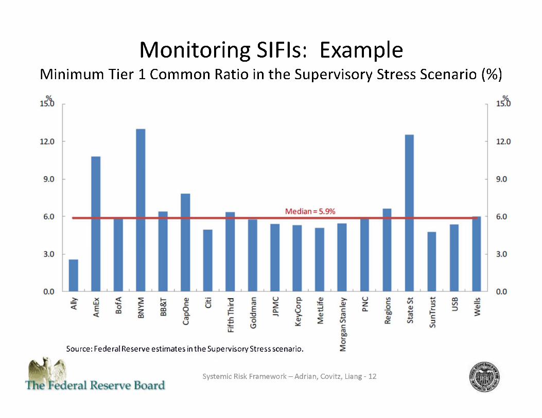
Monitoring SIFIs: Example Minimum Tier 1 Common Ratio in the Supervisory Stress Scenario (%)

[bar graph displaying the percentages held by different banks. The median of all banks is 5.9%. Ally is about 2.5%, AmEx is about 10.75%, BofA is about 5.8%, BNYM is about 13%, BB&T is about 6.5%, CapOne is about 7.75%, Citi is about 5%, Fifth Third is about 6.2%, Goldman is about 5.7%, JPMC is about 5.5%, KeyCorp is about 5.4%, MetLife is about 5.1%, Morgan Stanley is about 5.6%, PNC is about 5.9%, Regions is about 6.7%, State St is about 12.5%, Sun Trust is about 4.75%, USB is about 5.4%, and Wells is about 6%.]

Source: Federal Reserve estimates in the Supervisory Stress scenario.

2. Shadow Bank Monitoring • Potential for Destabilizing Drops in Asset Prices.

- Shadow banking could inflate asset valuations in booms and amplify asset price crashes in busts.

- Price and non-price measures of potential bubbles, extremely low volatility.

• Leverage Cycle, Maturity Mismatch, and Run Risk. - Measures of leverage in financial system (including on and off balance sheet

exposures). - Measures of maturity mismatch and vulnerability. - Hedge funds, insurers, pension funds, and other financial firms that are not SIFIS. - Activities not backed by government backstops: MMFs, cash pools, securities lending /

repo activities, velocity of collateral, securitization.

• New Products.

Monitoring Shadow Banking: Example Forward Credit Spreads

Near- and Far-Term BB Forward Credit Spreads Percent

[Graph plotting two lines: Near-term (Forward spread between years two and three) and Far-term (forward spread between years nine and ten). The latest daily observation was January 13, 2012. The graph starts in 1989. Near term starts at about 1.5%, goes up to about 6% in late 1992, is down to about 1.5% again in early 1995, makes its way up to about 7% in 2002, then down to about 1% in 2005, then peaks at about 15.5% in early 2009, then ends January 13, 2012 at about 5.5%. Far-term starts 1989 at about 3%, then is down to about 1% in 1992, then stays between there and 3% until 2000 when it is up to about 3.5%. It goes up to about 4.5% in early 2003, then is back down to staying between about 2 and 3.5% until mid 2008, when it rises and peaks at about 8% in early 2009. It drops again and ends January 13, 2012 at about 3.5%.]

Source. Staff estimates.

Monitoring Shadow Banking: Example Junk Bond Issuance

Gross Junk Issuance and Share of Deep Junk Issuance [graph from 1989 through 2011 plotting two lines: the billions of dollars of Gross junk Insurance (Includes public, 144a, euro, and MTN issues) and the percent of Deep Junk Share (Fraction of bonds rated B- or lower over total non-financial junk insurance). Gross Junk Insurance starts 1989 at about $5billion. It is down to about $1billion in 1990 . Then it heads up, hitting about $15 billion in 1993. Then it goes down to about $3 billion in 1994, then makes its way up, hitting about $44 billion in 1998. then down again, hitting about $4 billion in early 2001, but then it jumps, hitting about $35 billion by mid 2001. By mid 2002 it is down to about $5 billion. In 2003 it is up to about $40 billion, then down to about $15 billion in 2005, then up to about $54 billion the end of 2006, then down to about $2 billion the end of 2008. Then up to about $65 billion the end of 2010, then ends 2011 Q4 at about $27 billion. Deep Junk Share starts 1989 at about 80%, but drops quickly, hitting about 20% by the second quarter of 1989. Then rises to about 50% but drops to about 4% by the end of 1990. Then it works its way up, reaching about 50% in 1994, 2% in 1995, 60% the end of 1995, then about 30% in 1996. About 57% in 1998, about 33% in 1999, then about 75% in 2000. Then a big drop to about 20% in 2001, up to about 64% by 2005, then down to about 40% by 2006, then up to about 77% in 2007, drops to about 20% in early 2009, then ends 2011 Q4 at about 37%.]

Source: Thomson-Reuters

Monitoring Shadow Banking: Example Prime Money Market Fund Exposures

MMF Holdings, Prime Exposure Billions of Dollars

Graph from January through December 2011 plotting three lines: France, Europe (ex-France), US, and Rest of World. France starts in January 2011 at about $250 billion, stays there until April, rises to about $280 billion by June 2011, then begins dropping, reaching about $50 billion by the end of 2011. Europe (ex-France) starts in January 2011 at about $610 billion, is up to abou$690 billion by June, then down to about $500 billion by the end of 2011. US starts in January 2011 at about $600 billion, goes down to about $540 billion in August, then up again, ending 2011 at about $630 billion. Rest of World stars in January 2011 at about $320 billion, stays around there until August, then rises a bit, ending 2011 at about $450 billion.]

Source: SEC form N-MFP.

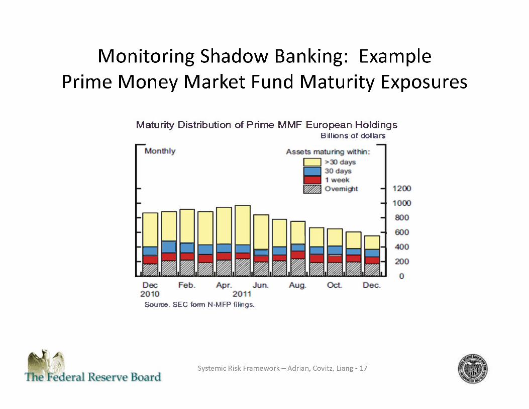
Monitoring Shadow Banking: Example Prime Money Market Fund Maturity Exposures

Maturity Distribution of Prime MMF European Holdings Billions of dollars

[bar graph from December 2010 through December 2011plotting four data: greater than 30 days, 30 days, 1 week, and overnight. In December 2010 Overnight was about $160 billion, 1 week about $120 billion, 30 days about $120 billion, and greater than 30 days about $450 billion. In January 2011 Overnight was about $210 billion, 1 week about $110 billion, 30 days about $180 billion, and greater than 30 days about $400 billion. In February 2011 Overnight was about $220 billion, 1 week about $100 billion, 30 days about $140 billion, and greater than 30 days about $550 billion. In March 2011 Overnight was about $190 billion, 1 week about $120 billion, 30 days about $130 billion, and greater than 30 days about $430 billion. In April 2011 Overnight was about $220 billion, 1 week about $100 billion, 30 days about $110 billion, and greater than 30 days about $500 billion. In May 2011 Overnight was about $240 billion, 1 week about $90 billion, 30 days about $110 billion, and greater than 30 days about $520 billion. In June 2011 Overnight was about $200 billion, 1 week about $90 billion, 30 days about $90 billion, and greater than 30 days about $420 billion. In July 2011 Overnight was about $210 billion, 1 week about $80 billion, 30 days about $110 billion, and greater than 30 days about $380 billion. In August 2011 Overnight was about $250 billion, 1 week about $130 billion, 30 days about $100 billion, and greater than 30 days about $350 billion. In September 2011 Overnight was about $190 billion, 1 week about $110 billion, 30 days about $100 billion, and greater than 30 days about $250 billion. In October 2011 Overnight was about $190 billion, 1 week about $110 billion, 30 days about $100 billion, and greater than 30 days about $220 billion. In November 2011 Overnight was about $200 billion, 1 week about $100 billion, 30 days about $90 billion, and greater than 30 days about $210 billion. In December 2011 Overnight was about $180 billion, 1 week about $90 billion, 30 days about $110 billion, and greater than 30 days about $180 billion.

Source. SEC form N-MFP filings.

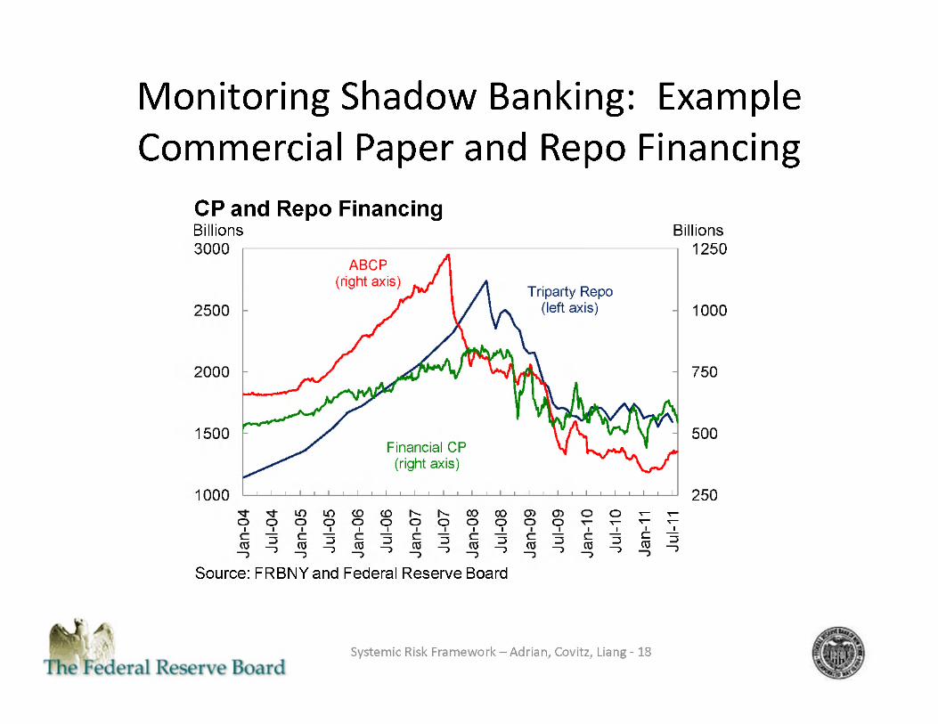
Monitoring Shadow Banking: Example Commercial Paper and Repo Financing

CP and Repo Financing Billions

[graph from January 2004 through July 2011 plotting three lines: ABCP, Triparty Repo, and Financial CP. ABCP starts January 2004 at about 675 billion, it goes up until around July 2007 when it peaks at about 1240 billion. Then it tends down, ending July 2011 at about 410 billion. Triparty Repo starts January 2004 at about 1150 billion, travels up until around April 2008 when it peaks at about 2750 bilion, Then it falls to about 1600 billion in January 2010 and stays around there, ending July 2011 at about 1600 billion. Financial CP starts January 2004 at about 550 billion. It goes up until around January 2008 when it reaches about 840 billion and stays around there until around October 2008, then drops to about 500 billion the end of July 2011 with jaggs of about 150 billion or so.

Source: FRBNY and Federal Reserve Board

Monitoring Shadow Banking: Example Shadow Banking Liabilities

Shadow Liabilities Trillions

[graph from 1990 through 2011 plotting three lines: Shadow Liabilities, Net Shadow Liabilities, and Bank Liabilities. Shadow Liabilities starts 1990 at about 3 trillion. It slopes up until it peaks in 2009 at about 21 trillion. Then it goes down to about 15 trillion in the beginning of 2011. Net shadow liabilities starts 1990 at about 2.5 trillion, It slopes up until it peaks in 2009 at about 16.5 trillion then slopes down to about 12.5 trillion in the beginning of 2011. Bank Liabilities starts 1990 at about 3 trillion. Then it slopes up and reaches the beginning of 2011 at about 13.25 trillion.]

Source: Flow of Funds

3. Real Economy Monitoring

• Nonfinancial sector risk.

- Leverage of nonfinancial sector—households, businesses,

governments.

- Nonfinancial credit that is ultimately funded with short-term debt.

• Effect of financial sector on economic activity.

- Underwriting standards, risk appetite, and balance sheet capacity of

financial institutions.

- Indicators of macro-economy vulnerability to financial risks.

Real Economy Monitoring: Example Nonfinancial Sector Credit-to-GDP Ratio

Nonfinancial sector credit-to-GDP ratio [graph from 1955 through 2011 Q3 plotting two lines: Nonfinancial Sector and Nonfinancial private sector. Nonfinancial private sector starts 1955 at about a ratio of 0.55. Then it rises fairly steadily until 1990 when it hits about a ratio of 1.25. Then it drops a bit, hitting a ratio of about 1.15 in 1994. Then it rises until it peaks in 2009 at a ratio of about 1.8. Then it drops to about 1.6 in 2011 Q3. Nonfinancial sector starts 1995 at a ratio of about 1.15. By 1961 it is up to a ratio of about 1.3, then stays around there varying no more than .1 until 1981 when it starts rising. It reaches a ratio of about 1.8 in 1991, then drops to about 1.7 in 2000, then rises to a peak of about 2.5 in 2009. It ends 2011 Q3 with a ratio of about 2.45. The graph indicates that the space between nonfinancial private sector and nonfinancial sector is govenrment. The space below nonfinancial private sector is divided roughly in half, with the bottom half being household and the top half being business.]

Source: FOFA and NIPA

Real Economy Monitoring: Example Senior Loan Officer Survey

Willingness to Make Consumer Installment Loans Percent

[graph from 1990 through 2011 Q4. When the data is above 0 it means more willing than 3 months ago. When the data is below 0 it means less willing than 3 months ago. It starts 1990 at about 10%, then passed through 0 at the end of 1990, and reached about -15% in early 1991. It passed back up through 0 in mid 1991. It peaks at about 30% in 1994, then goes down and passes through 0 in 1996, reaching about -5% by the end of 1996. Then up through 0 in 1997, reaching about 13% in 1999. It passes through 0 in 2000, and reaches about -7% in early 2002. Up through 0 in late 2002, reaching about 20% in early 2006. Then down through 0 in 2007, reaching an ultimate low of about -48% in late 2008. Then up through 0 in 2010, peaking at about 30% in 2011. It ends 2011 Q4 at about 17%.]

Note: Net percent of banks reporting willingness to make loans. Source: Senior Loan Officer Opinion Survey on Bank Lending Practices.

Conceptual Framework for Policy Response to Systemic Risk

• Monitoring indicates the extent to which shocks might trigger systemic events.

- Monitoring informs us about exposures to changes in the pricing of risk.

- Sharp increases in the pricing of risk can generate systemic risk.

• Tradeoff between systemic risk and the price of risk.

- Regulation is trading off the price of risk with the level of systemic risk.

- Higher price of risk today may reduce buildup of systemic risk.

• Tougher regulation, higher price of risk, less systemic risk.

Ex ante Policies to Promote Financial Stability

1. SIFIs. - Size of macroprudential surcharge. - Stringency of capital requirements, and liquidity requirements.

2. Shadow Banking. - Margins , more centralized clearing. - MMMF and repo reforms. - Greater disclosure and transparency, better accounting.

3. Nonfinancial sector. - Lender restrictions. - Borrower requirements.

Research Agenda for Measuring Interconnectedness

Sean Campbell

These slides present the author's perspective on ongoing research related to the measurement of interconnectedness. The views expressed herein are solely the author's, and do not reflect those of the Federal Reserve Board or its staff. All information

presented here is publicly available.

Outline

• Brief overview of near term policy initiatives that call for concrete measures of interconnectedness.

• Research perspective on interconnectedness measures.

• Discussion of how interconnectedness relates to other important research/policy initiatives.

• Directions for future research.

Near Term Policy Initiatives • A number of specific policy initiatives require concrete measures of interconnectedness.

1. FSOC determination of non-bank SIFI's. • Proposed rule issued by FSOC 10/2011.

• Proposal states that "The Council intends to evaluate a broad group of nonbank financial companies by applying uniform quantitative thresholds representing the framework categories that are more readily quantified, namely size, interconnectedness ... A nonbank financial company would be subject to additional review if it meets both the size threshold and any one of the other quantitative thresholds.".

2. Evaluation of systemic risk consequences of significant bank mergers. • Evaluations are currently underway (CapOne and ING).

• Evaluation will consider "a variety of metrics. These would include measures of the size of the resulting firm;.... interconnectedness of the resulting firm with the banking or financial system".

Near Term Policy Initiatives

• Interconnectedness is not simply one of many small dimensions of the problem that must be assessed. Rather it is seen as being critical to these near term initiatives.

• Consider the FSOC proposed rule on identifying non-bank SIFI's.

1. Interconnectedness is identified as one of six key elements defining a non-bank SIFI.

2. Commenters view this element as being, perhaps, the most important of the six complementary elements.

"Many commenters expressed the view that interconnectedness with the broader financial system is the most important indicator of a nonbank financial company's potential to pose a threat to U.S. financial stability." - FSOC proposed rule.

Research Perspective on IC Measures • How should "interconnectedness" be defined? What is a useful working definition?

• The FSOC proposed rule provides one candidate definition.

"[interconnectedness is an assessment of] the potential impact of a [non-bank financial] company's financial distress on the broader economy".

• How does financial distress translate into a real effect (i.e. lost output) on the broader economy (i.e. both inside and outside the financial sector).

• The key issue is to think about trying to measure how financial distress leads to real negative effects on other firms, industries and sectors.

• Measured against this working definition of interconnectedness how well do existing measures quantify the important elements of interconnectedness????

Research Perspectives on IC Measures • Many extant measures of IC focus heavily on measuring the potential size of financial

distress that a given firm might experience.

e.g. Systemic Expected Shortfall (SES) Acharya et. al. (2010) - "each financial institu-tion's contribution to systemic risk can be measured as its systemic expected shortfall (SES), i.e., its propensity to be undercapitalized when the system as a whole is un-dercapitalized. SES increases with the institution's leverage and with its expected loss in the tail of the system's loss distribution."

• These types of measures are useful for measuring the size and significance of financial distress but it is not clear how such financial distress can be mapped into outcomes for the broader economy.

• Could the failure (near failure) of the firm be absorbed by the rest of the economy? • Could other competitors fill the void for the period of time that the firm is under

financial stress? • How important are the services of the firm to the rest of the economy?

Research Perspectives on IC Measures • Understanding how financial distress in one firm/industry/sector feeds forward through

the rest of the economy is a significant research challenge.

• The inter-relationships between different aspects of the financial sector and the broader economy is complex and multi-faceted.

• Consider all of the following sub-sectors of the financial sector that play a role in the broader economy.

prime brokerage, underwriting, securities lending, clearing services, SME lending, insurance, reinsurance, asset management,.

• The linkages between these sectors and the rest of the financial sector as well as the broader economy are not well understood in a systematic and quantifiable manner.

• Measures that focus on characterizing the size and significance of financial distress in these (and other) industries fall short of the mark. Ultimately, IC measures need to make a systematic and quantifiable connection to the unavoidable fallout from such financial dis-locaton.

Research Perspectives on IC Measures • Understanding and quantifying the degree of uncertainty around IC measures is

important for having the appropriate perspective on the signal strength of any particular measure. It may also tell us which components of IC may hold more promise for measurement.

MES Predicts Realized Equity Returns During the Crisis

Research Perspectives on IC Measures • Understanding and quantifying the degree of uncertainty around such IC measures is

important for having the appropriate perspective on the signal strength of any particular measure. It may also tell us which components of IC may hold more promise for measurement.

MES Predicts Realized Equity Returns During the Crisis

[scatter plot. X axis is MESS measured June 06 to June 07, with values 0 to .04. Y axis is Return during crisis: July 07 to Dec 08, with values -1 to .5. The trend line starts at the left at about .004, -.25 and moves down to about .033, -.75. Most of the data fall between .01 and .02 on the X axis, and between -1 and 0 on the Y axis.]

• Tail events are notoriously hard for anyone/thing to forecast. Other aspects of IC may be more amenable to stable and systematic quantification

Relation of Interconnectedness to Other Initiatives

• Interconnectedness is an important concept for broadening our understanding of how different aspects/sectors of the economy function together.

• Understanding how different financial activities relate to the broader economy is a key part of understanding the economics of financial stability.

• How does the financial sector play a role in our understanding of the near-tem evolution of the macroeconomy? (Macro Modeling - Kiley).

•What are the feedback effects to other banks and FI's in the event that one particular financial institution is impaired? (Macroprudential Stress Tests - Lehnert).

Directions for Future Research Modeling and measurement of interconnectedness is in its infancy. Lots of promising avenues for future research. A few that come to mind include:

• Thinking through how to quantify the real effects of financial distress across the broader economy.

• What are the best measures/indicators of "connection" to other firms and sectors? Credit or other services provided? Number of counterparties? Ease of substitution?

• Network models - a number of "first generation" network models (e.g Gai et. al. (2011)) are promising but lack realism in network dynamics.

• What are the determinant of network formation? • How do networks change in the event of information or stress events? • What are the conditions that lead to the formation of fragile/robust networks?

Research Agenda for Stress Testing

Andreas Lehnert

These slides present the author's perspective on ongoing research related to stress testing and other supervisory activities. The views expressed herein are solely the author's, and do not reflect those of the Federal Reserve Board or its staff. All information

presented here is publicly available.

Outline

• Overview of generic stress testing process • Research perspective on the 2012 exercise • Directions for future research

— Information collections

Process overview

[flow chart. Design to Macro scenario to Top-down loss estimates to Bottom-up loss estimates to capital trajectory to disclosure.]

[about] Design elements: What data to collect. Standard for pass/fail; actions tied to results. Evolution of balances/RWA. Other assumptions (e.g. riskiness of newly originated loans). Macroprudential elements?

[about] Scenario design: Variables to include? Severity? Separate trading shock.

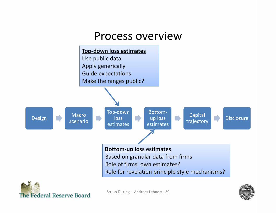
[about] Top-down loss estimates: Use public data. Apply generically. Guide expectations. Make the ranges public?

[about] Bottom-up loss estimates: Based on granular data from firms. Role of firms' own estimates? Role for revelation principle style mechanisms?

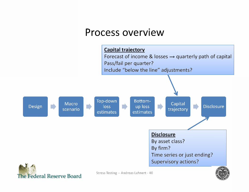
[about] Capital trajectory: Forecast of income & losses to quarterly path of capital. Pass/fail per quarter? Include "below the line" adjustments?

[about] Disclosure: By asset class? By firm? Time series or just ending? Supervisory actions?

RESEARCH PERSPECTIVE ON THE 2012 EXERCISE

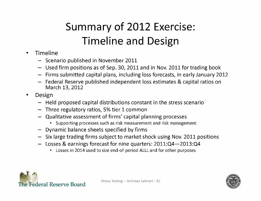
Summary of 2012 Exercise: Timeline and Design

• Timeline: - Scenario published in November 2011. - Used firm positions as of Sep. 30, 2011 and in Nov. 2011 for trading book. - Firms submitted capital plans, including loss forecasts, in early January 2012. - Federal Reserve published independent loss estimates & capital ratios on

March 13, 2012. • Design:

- Held proposed capital distributions constant in the stress scenario. - Three regulatory ratios, 5% tier 1 common. - Qualitative assessment of firms' capital planning processes.

• Supporting processes such as risk measurement and risk management. - Dynamic balance sheets specified by firms. - Six large trading firms subject to market shock using Nov. 2011 positions. - Losses & earnings forecast for nine quarters: 2011:Q4—2013:Q4.

• Losses in 2014 used to size end-of-period ALLL and for other purposes.

Summary of 2012 Exercise: Scenario, Loss Estimates & Disclosure

• Scenario - U.S. enters a severe recession - Unemployment rate 13%, house prices -21% - GDP and exchange rates for country/country blocks - Trading shock reflected widening in sovereign spreads

• Loss estimates - No top-down loss estimates distributed - Wholesale, retail, AFS-HTM - Trading book & PPNR - Bottom-up independent loss estimates published

• Disclosure - Firm-specific results - Minimum and period-end capital ratios

Scenario Unemployment Rates [graph plotting four lines from 2006 through 2014: Data, SCAP (interpolated), CCAR, and CCAR 2012. The Data line starts 2006 at about 4.8%, and stays between there and about 4.5% through mid 2007. Then it starts to rise, reaching about 7% in the beginning of 2009, and maxing at about 10% in the end of 2009. Then it slopes down, ending at about 8.5% in early 2012. The SCAP (interpolated) line starts in late 2008 at about 6.8%, rises up to about 10.2% in the beginning of 2010, then ends early 2011 at about 10.5%. The CCAR line starts in mid 2010 at about 9.5%, rises to a maximum of about 11.2% in early 2012, then ends the beginning of 2014 at about 9.5%. The CCAR 2012 line starts around mid 2011 at about 9%, then rises to a maximum of about 13% in early 2013, then ends the end of 2014 at about 11.5%.]

Two-year Loan Loss Rates Commercial Banks

1920-2011

[Graph plotting the two-year loan loss rates of commercial banks from 1921 through 2011. It shows reference lines SCAP (2009) at about 9 throughout, and CCAR 2012 at about 7.2 throughout. The rates start at about 1.5 in 1921. By about 1930 they were down to about 0.8. Then a big spike around 1934 to about 8.7. Then a sharp decline to about 1 in 1937, then it continues dropping, reaching about -.3 in 1945. Then a slow rise, reaching about .3 in 1969. Then a rise to about 1.3 in 1976. Then a drop to about .6 in 1979. Then a rise, reaching about 3 in 1991. Then a drop to about 1 in 1995. Then a rise to about 2 in 2004, then a drop to about 1 in 2006. Then a rise, reaching about 5.3 in 2010 and ending 2011 at about 4.2.]

Stylized Representation of Capital Analysis

[bar graph plotting four data: starting capital ratio, losses in stress scenario, proposed capital distribution, and post-stress capital ratio. The Starting capital ratio is a bar spanning about 0 to 14. The Losses in stress scenario is a bar spanning about 10 to 14, with a note "Minimum stressed ratio assuming no capital actions after Q1 2012". The Proposed capital distribution is a bar spanning about 7.5 to about 10, with a note"Minimum stressed ratio with all proposed capital actions through Q4 2013". The Post-stress capital ratio is a bar spanning about 0 to 7.5.]

DIRECTIONS FOR FUTURE RESEARCH

Number of journal articles containing the search term in their abstracts (1980 to 2011)

Journals Covered: Journal of Finance; Journal of Political Economy; American Economic Review; Quarterly Journal of Economics; Econometrica; Review of

Economic Studies

[bar graph showing Monetary policy at about 120, (bank and super" or macroprudential at about 3, and great moderation at about 4.]

Information Collections

• Understand what information supervisors are collecting. — And what might be feasible alternatives.

• Information collected (generally) using public regulatory reports.

• Changes to reports typically associated with public notice and comment.

[image of the federal reserve home page: http://www.federalreserve.gov, pointing out the header "reporting forms".]

Image of the federal reserve's website "reporting forms" page, pointing out the link for "Information collections under review".]

[image of the table on the Information Collections under review page, pointing out the line with reporting form numbers FR Y-14A, FR Y-14M, and FR Y-14Q.]

Current information collection FR Y-14Q & FR Y-14M

• PPNR. - Actual balances & rates earned on assets by category (first-lien, C&I,...). - Non-interest income/expenses. - Weighted average life of assets/liabilities. - Retail repricing "beta" (sensitivity of cost of funds to rate shocks).

• Retail (mortgages, cards, auto, ...). • Wholesale (C&I, CRE loans, ...). • Securities (financial assets held in AFS/HTM portfolio). • Trading.

- Sensitivities of assets to shocks (DV01, CS01, vega). - Counterparty credit risk exposures (CVA, IDR, top 10 lists).

• Basel III. • Regulatory capital instruments.

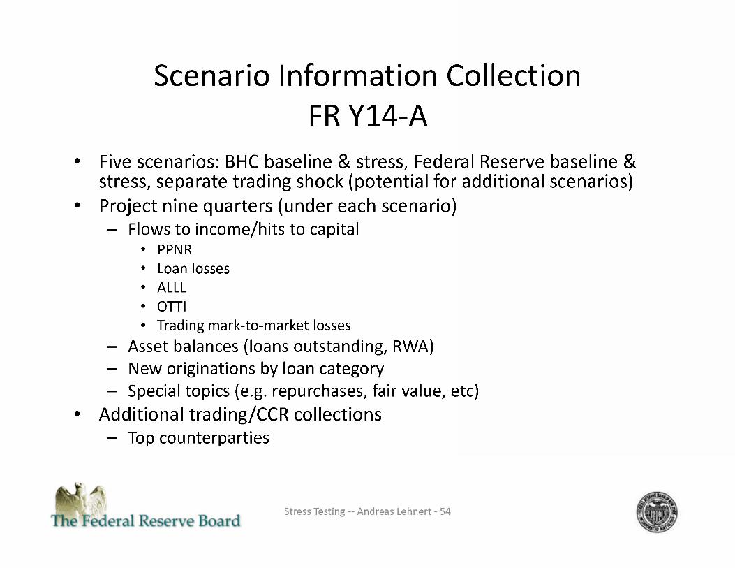
Scenario Information Collection FR Y14-A

• Five scenarios: BHC baseline & stress, Federal Reserve baseline & stress, separate trading shock (potential for additional scenarios).

• Project nine quarters (under each scenario). - Flows to income/hits to capital.

• PPNR. • Loan losses. • ALLL. • OTTI. • Trading mark-to-market losses.

- Asset balances (loans outstanding, RWA). - New originations by loan category. - Special topics (e.g. repurchases, fair value, etc).

• Additional trading/CCR collections. - Top counterparties.

Research Directions

• Micro/product-specific analysis. - Loss forecasting. - Elasticity of demand. - Behavior in tail events. - Better information to collect.

• Trading and counterparty credit risk. - Designing scenarios. - Counterparty behavior in stress episodes.

• Macro topics. - Designing scenarios. - Role of bank capital in macro outcomes (e.g. countercyclical capital buffers).

• Banking. - Cost of bank liabilities. - Determinants of bank risk appetites.

• Research on supervision. - Connection to program evaluation literature. - Study of forecast errors. - Alternative approaches (including information collection). - Alternative targets. - Disclosure policy. - New form of supervision (public, quantitative, ...).

Macroeconomic Modeling of Financial Intermediation:

A Review of Tools Used at the Federal Reserve Board and Their

Relation to Ongoing Research

Michael Kiley

These slides present the author's perspective on ongoing research related to macroeconomic modeling. The views expressed herein are solely the author's, and do not reflect those of the Federal Reserve Board or its staff

Macroeconomic Models at the Federal Reserve Board

• Staff at the Federal Reserve use many "models".

• "Models" are used in a wide variety of contexts.

• Perhaps most importantly, "models" are tools that are widely used, but no single model "rules the day", and model results are just one input into forecasting and policy analysis.

• In the remainder of this presentation, I will mainly focus on "structural" macroeconomic models used for forecasting and policy analysis, with a tilt toward models that address issues related to financial intermediation.

- I will focus (almost) exclusively on models used at the Federal Reserve or other central banks, either systematically or on certain projects (including research projects).

- As a result, this review of models leaves out many important academic contributions that have helped shape the approaches taken by researchers at central banks.

Macroeconomic Models at the Federal Reserve Board

• Staff at the Federal Reserve use many "models".

- Simple-to-complex time series models.

- Small, "semi-structural" models capturing key relationships that can bring out the intuition behind results (e.g., Fuhrer-Moore (1995), Rudebusch-Svensson (1999) models).

- A mix of calibrated/estimated dynamic general equilibrium models (e.g., like EDO (Edge, Kiley, Laforte (2008), Chung, Kiley, Laforte (2010) and SIGMA (Erceg, Guerrieri, and Gust (2006)).

- Larger "structural" models (FRB/US (Brayton and Tinsley (1997)).

Macroeconomic Models at the Federal Reserve Board

• "Models" are used in a wide variety of contexts.

- To assist staff analyses and research of monetary policy issues, including. • The production of forecasts. • The estimation of latent variables (e.g., "the output gap", "the state of the business

cycle"). • The assessment of the effects of monetary policy strategies.

- To analyze the implications of other policies (e.g., fiscal policies). Such analyses. • Aid monetary policy analyses, contribute to public discussions of the effect of such

actions, and engage related research. • Examples: Elmendorf and Reifschneider (2002), Coenen et al (2012).

- To analyze issues related to financial stability. • The use of "macroeconomic" models to consider issues related to financial stability is

increasing, and basic research is a significant part of these analyses. • Example: Macroeconomic Assessment Group reports (BIS (2010)).

Structural Macroeconomic Models: A Review of Common Approaches

• A variety of "structural" models are used for forecasting and policy analysis. • Financial conditions in a large number of central bank models share a Neoclassical view of

financial conditions (as discussed in Boivin, Kiley, and Mishkin (2011).

Small, Semistructural (many examples, e.g., Fuhrer and Moore (1995))

FRB/US (Brayton and Tinsley (1997)

EDO (Edge, Kiley, Laforte (2008), Chung, Kiley, Laforte (2010))

SIGMA (Erceg, Guerrieri, Gust (2006))

Loosely motivated equations

Equations reflect explicit dynamic adjustment problem

DSGE model, firm/ household optimization (specific functional forms)

DSGE model, firm/ household optimization (specific functional forms)

Perhaps an IS curve, Phillips curve, and interest rate rule

Very large (hundreds of equations)

Medium-sized (less than 100 equations)

Multicountry versions can be very large --medium/small per country

Rational expectations Reduced-form or Rational expectations

Rational expectations Rational expectations

Neoclassical view of financial conditions (EH)

Largely Neoclassical view of financial conditions

Largely Neoclassical view of financial conditions

Largely Neoclassical view of financial conditions

Frictionless financial intermediation

Largely frictionless financial intermediation, exog. risk premiums

Largely frictionless financial intermediation, exog. risk premiums

Largely frictionless financial intermediation, exog. and endog. risk premiums

Incorporating Financial Frictions into Macroeconomic Models - Exogenous Shocks

• Fluctuations in financial frictions play a key role in how policy models are used. - In EDO, exogenous fluctuations in a risk premium account for the lion's share of macroeconomic

fluctuations. - In SIGMA, key risks from international conditions often are modeled as exogenous fluctuations in a

risk premium (for example, on dollar assets (e.g., flight-to-safety movements) or foreign private-sector borrowing rates).

• Emphasis on exogenous movements in risk premiums reflects both the simplicity of the models and the fact that amplification of other shocks through fluctuations in risk premiums is often moderate (or less) in such models (e.g., Boivin, Kiley, and Mishkin (2011).

• Modeling of exogenous risk premiums - some exogenous factor (X(t)) that drives a wedge between the return on a risk-free asset and the return to investors in a private asset (e.g., physical capital, residences, consumer durables).

- Example: Smets Wouters (2007) risk-premium shock (e.g., most important shock in EDO). 1 = EtM (t +1) R( t +1) X (t +1)

- Increase in risk premium leads to lower consumption and investment.

Incorporating Financial Frictions into Macroeconomic Models - Endogenous Frictions

• Frameworks popular for modeling behavior of households or nonfinancial firms. - Collateral Constraints (e.g., loan-to-value constraints for housing, Iacoviello (2005)). Debt

must be less than some fraction of the market value of an asset.

B(t) less than or equal to mu Q(t) K(t).

• A tighter collateral constraint - reflecting, for example, a decline in asset values (Q(t)) or exogenous shocks to collateral constraint (i.e., change in loan-to-value required, etc.) -depresses investment and consumption by the constrained household.

- Financial Accelerator (e.g., Bernanke-Gertler-Gilchrist (1999)). Debt financing limited by net worth of borrower.

1 = Et (M(t +1)R(t +1)).

Q(t)= Et ((M(t+1))divided by (X(t+1))(MPK(t+1)+Q(t+1))).

EtX(t+1) = F((N(t+1))divided by (Q(t)K(t+1))).

• A decline in asset values boosts spread (X), lowers investment; similar implications for some exogenous shocks, such as an increase in idiosyncratic risk of investment projects.

Incorporating Financial Frictions into Macroeconomic Models - Some Important Challenges

• Extensions to models of intermediation. - Use models of frictions for nonfinancial firms to think about intermediaries. - Example: Impose a capital/leverage constraint on intermediaries, much in the same way

an exogenous collateral constraint might be imposed, to think about influence of balance sheet conditions for macroeconomic outcomes.

• Such extensions need to think about special features of intermediaries. For example, intermediaries.

- Finance investment and provide liquidity services. - Have access to cheap debt-like financing because of liquidity services associated with

deposits/short-term liabilities, taxes, or other features - creating high leverage. - Engage in maturity transformation - financing long-term investment (lending) using

short-term liabilities.

Incorporating Financial Frictions into Macroeconomic Models - A Model of Intermediation

• A model of intermediaries in the presence of financial frictions (Kiley and Sim (2011), (2012)). - Intermediaries are essential - households direct investment activities through intermediaries. - Debt financing is cheap (liquidity services, tax preference), but bankruptcy is costly (limited

recovery). - Internal funds cheaper than external funds (e.g., costly to issue equity). - Maturity mismatch - timing of returns creates funding risk, yielding time-variation in the value of

cash on the balance sheet and hence willingness to lend (precautionary behavior). - Implications: Capital policy that trades off benefits of debt financing and the risk of having to raise

external funds.

• Key equation and implications: Pricing equation for lending rate. - M(t+1)X(t+1) is the stochastic discount factor of the intermediaries, which prices assets throughout

the economy as household savings are channeled through intermediaries.

1 = EtM(t +1) R( t +1) X( t +1).

• Similar to He and Krishnamurthy (2010), who assume risk-averse intermediaries. • Precautionary behavior of intermediaries reflects mis-match between assets and liabilities -

lending commitments that cannot be unwound in response to changes in value of assets. • Key role for "willingness to lending " (e.g., Lown and Morgan (2006)).

Incorporating Financial Frictions into Macroeconomic Models -Some Model Implications

• Willingness to lend is adversely affected by any adverse shift in balance sheet condition/risk

[an illustration showing 12 small graphs with infinite slopes. The graphs are too small to make out any data.]

Incorporating Financial Frictions into Macroeconomic Models -Some Model Implications (2)

• Crisis policies - capital injections differ from asset purchases because of crowding out

[an illustration showing 9 small graphs with infinite slopes. The graphs are too small to make out any data.]

Incorporating Financial Frictions into Macroeconomic Models -Some Model Implications (3)

• Transition to Basel 3 - slow transition may lower transition effects by facilitating capital accretion using internal funds

[an illustration showing 9 small graphs with infinite slopes. The graphs are too small to make out any data.]

Incorporating Financial Frictions into Macroeconomic Models - Further Examples

• Crisis policies such as. - Capital injections vs. asset purchases (Kiley and Sim (2011, 2012)). - Government-financed intermediation (Gertler and Karadi (2011,2012)).

• Implementation of Basel 3 (BIS (2010), Kiley and Sim (2011)).

• Research questions relating to macroprudential regulation. - Stabilization properties of policies that adjust capital requirements in response to credit

indicators (e.g., Christensen, Meh, and Moran (2011)). • This research investigates questions raised by, for example, the Basel 3 countercyclical capital

buffer proposals from the BIS (for a discussion and references, see Edge and Meisenzahl (2011)). • Examine alternative macroprudential approaches - e.g., leaning against financing spreads (Kiley

and Sim (2012)).

- Cyclical adjustment of loan-to-value ratios. • Leaning against the wind through LTV adjustments may ameliorate housing cycles (Lambertini

et al (2011)).

Incorporating Financial Frictions into Macroeconomic Models - Some Important Challenges

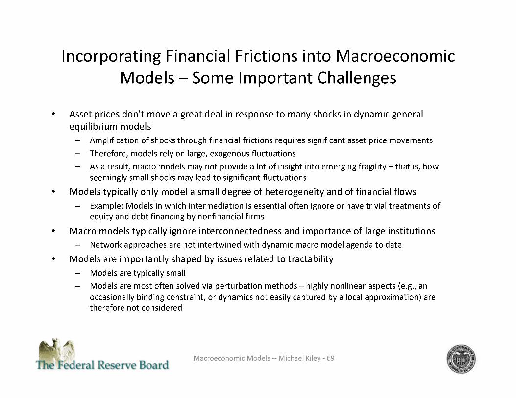
• Asset prices don't move a great deal in response to many shocks in dynamic general equilibrium models.

- Amplification of shocks through financial frictions requires significant asset price movements. - Therefore, models rely on large, exogenous fluctuations. - As a result, macro models may not provide a lot of insight into emerging fragility - that is, how

seemingly small shocks may lead to significant fluctuations.

• Models typically only model a small degree of heterogeneity and of financial flows. - Example: Models in which intermediation is essential often ignore or have trivial treatments of

equity and debt financing by nonfinancial firms.

• Macro models typically ignore interconnectedness and importance of large institutions. - Network approaches are not intertwined with dynamic macro model agenda to date.

• Models are importantly shaped by issues related to tractability. - Models are typically small. - Models are most often solved via perturbation methods - highly nonlinear aspects (e.g., an

occasionally binding constraint, or dynamics not easily captured by a local approximation) are therefore not considered.

References

Bernanke, Ben S., Gertler, Mark, Gilchrist, Simon (1999) The financial accelerator in a quantitative business cycle framework. Handbook of Macroeconomics. 1341-1393 http://ideas.repec.org/h7eee/macchp/1-21.html

BIS (2010). Assessing the macroeconomic impact of the transition to stronger capital and liquidity requirements. Interim report of the

macroeconomic assessment group, Basel Committee on Banking Supervision, Basel, Switzerland. http://www.bis.org/press/p100818.htm

Boivin, J., M. T. Kiley, and F. S. Mishkin (2010). How has the monetary transmission mechanism evolved over time? Volume 3 of Handbook of

Monetary Economics, pp. 369 - 422. Elsevier. http://ideas.repec.org/h/eee/monchp/3-08.html

F. Brayton and P. Tinsley (1996) A guide to FRB/US: a macroeconomic model of the United States. Finance and Economics Discussion Series. Board of Governors of the Federal Reserve System (U.S.) http://ideas.repec.org/p/fip/fedgfe/96-42.html

Hess T. Chung, Michael T. Kiley, Jean-Philippe Laforte (2010) Documentation of the Estimated, Dynamic, Optimization-based (EDO) model of the U.S. economy: 2010 version. Finance and Economics Discussion Series Board of Governors of the Federal Reserve System (U.S.) http://ideas.repec.org/p/fip/fedgfe/2010-29.html

Christensen, I., C. Meh, and K. Moran (2011). Bank leverage regulation and macroeconomic dynamics. Cahiers de recherche 1140, CIRPEE. http://ideas.repec.org/p/bca/bocawp/11-32.html

Coenen, Gunter, et al (2012_. "Effects of Fiscal Stimulus in Structural Models." American Economic Journal: Macroeconomics, 4(1): 22-68.

http://www.aeaweb.org/articles.php?doi=10.1257/mac.4.1.22

Edge, Rochelle M., Kiley, Michael T., Laforte, Jean-Philippe (2008) Natural rate measures in an estimated DSGE model of the U.S. economy. Journal

of Economic Dynamics and Control. 32:2512-2535. http://ideas.repec.org/a/eee/dyncon/v32y2008i8p2512-2535.html

Edge, R. M. and R. R. Meisenzahl (2011, December). The unreliability of credit-to-gdp ratio gaps in real time: Implications for countercyclical capital buffers. International Journal of Central Banking 7(4), 261-298.

Elmendorf, Douglas W. and David Reifschneider. 2002. "Short Run Effects of Fiscal Policy with Forward-Looking Financial Markets." National Tax Journal, 55(3). September. Christopher J. Erceg , Luca Guerrieri, Christopher Gust (2006)SIGMA: A New Open Economy Model for Policy Analysis. International Journal of Central Banking 2 http://ideas.repec.org/a/iic/ijcjou/y2006q1a1.html

Fuhrer, Jeffrey C, Moore, George R (1995)Monetary Policy Trade-offs and the Correlation between Nominal Interest Rates and Real Output.

American Economic Review 85:219-39 http://ideas.repec.org/a/aea/aecrev/v85y1995i1p219-39.html

Gertler, M. and P. Karadi (2011). A model of unconventional monetary policy. Journal of Monetary Economics 58(1), 17 - 34. Carnegie-Rochester

Conference Series on Public Policy: The Future of Central Banking April 16-17, 2010.

He, Zhiguo and Arvind Krishnamurthy. 2010. Intermediary Asset Pricing. http://www.kellogg.northwestern.edu/Faculty/Directory/Krishnamurthy Arvind.aspx#research

Matteo Iacoviello (2005) House Prices, Borrowing Constraints, and Monetary Policy in the Business Cycle. American Economic Review 95:739- 764 http://ideas.repec.org/a/aea/aecrev/v95y2005i3p739-764.html

References

Michael T. Kiley and Jae W. Sim (2011) Financial capital and the macroeconomy: policy considerations. Finance and Economics Discussion Series. Board of Governors of the Federal Reserve System (U.S.) http://ideas.repec.org/p/fip/fedgfe/2011-28.html

Michael T. Kiley and Jae W. Sim (2012) Intermediary Leverage, Macroeconomic Dynamics, and Macroprudential Policy. Draft,

http://www.ecb.int/events/conferences/shared/pdf/researchforum7/Sim Jae.pdf?ea43fd66e6ccff2bfba5a052bece007c

Luisa Lambertini, Caterina Mendicino and Maria Teresa Punzi (2011) "Leaning Against Boom-Bust Cycles in Credit and Housing Prices" Center for Fiscal Policy Working Paper Series, Working Paper 01-2011 http://ideas.repec.org/p/cif/wpaper/201101.html

Lown, Cara & Morgan, Donald P., 2006. "The Credit Cycle and the Business Cycle: New Findings Using the Loan Officer Opinion Survey," Journal of Money, Credit and Banking, Blackwell Publishing, vol. 38(6), pages 1575-1597, September. http://ideas.repec.org/a/mcb/jmoncb/v38y2006i6p1575-1597.html

Glenn Rudebusch, Lars E.O. Svensson (1999) Policy Rules for Inflation Targeting . NBER Chapters, National Bureau of Economic Research, Inc http://ideas.repec.org/h/nbr/nberch/7417.html

Frank Smets, Rafael Wouters (2007)Shocks and Frictions in US Business Cycles: A Bayesian DSGE Approach. American Economic Review 97:586-606

http://ideas.repec.org/a/aea/aecrev/v97y2007i3p586-606.html

Viaral Acharya, Lasse Pedersen, Thomas Phillipon and Matthew Richardson (2010). "Measuring Systemic Risk". Draft.

http://pages.stern.nyu.edu/~sternfin/vacharya/public html/~vacharya.htm

Financial Stability Oversight Council, "Authority to Require Supervision and Regulation of Certain Nonbank Financial Companies". 12 CFR Part 1310

http://www.gpo.gov/fdsys/granule/FR-2011-10-18/2011-26783/content-detail.html

Federal Reserve System, "Order Approving the Acquisition of a Savings Association" and Nonbanking Subsidiaries". http://www.gpo.gov/fdsys/granule/FR-2011-10-18/2011-26783/content-detail.html

Board of Governors of the Federal Reserve System (2012), Comprehensicve Capital Analysis and Review 2012: Methodology for Stress Scenario Projections http://www.federalreserve.gov/newsevents/press/bcreg/bcreg20120312a1.pdf