January 2013

Federal Regulation and Aggregate Economic Growth

John W. DawsonDepartment of Economics

Appalachian State UniversityBoone, NC, 28608-2051dawsonjw@appstate.edu

John J. SeaterDepartment of Economics

North Carolina State UniversityRaleigh, NC, 27695

john_seater@ncsu.edu

Abstract

We introduce a new time series measure of the extent of federal regulation in the U.S. and use it toinvestigate the relationship between federal regulation and macroeconomic performance. We find that regulationhas statistically and economically significant effects on aggregate output and the factors that produce it–total factorproductivity (TFP), physical capital, and labor. Regulation has caused substantial reductions in the growth rates ofboth output and TFP and has had effects on the trends in capital and labor that vary over time in both sign andmagnitude. Regulation also affects deviations about the trends in output and its factors of production, and the effectsdiffer across dependent variables. Regulation changes the way output is produced by changing the mix of inputs. Changes in regulation offer a straightforward explanation for the productivity slowdown of the 1970s. Qualitativelyand quantitatively, our results agree with those obtained from cross-section and panel measures of regulation usingcross-country data.

Keywords: Regulation; macroeconomic performance; economic growth; productivity slowdown.

JEL classification: E20; L50; O40

We thank Michele Boldrin, Tim Bollerslev, Michelle Connolly, Simeon Djankov, Ronald Gallant, ThomasGrennes, Bruce Hansen, Bang Jeon, Christopher Laincz, Oksana Leukhina, Aart Kraay, John Lapp, Marcelo Oviedo,Douglas Pearce, Denis Pelletier, Pietro Peretto, Martin Rama, George Tauchen, an anonymous referee, and ananonymous Associate Editor for helpful comments. We are also grateful to Amit Sen for providing finite-samplecritical values for the Zivot-Andrews test. The regulation and marginal tax rate data are available on Seater’swebsite at: http://www4.ncsu.edu/~jjseater/index_003.htm.

1. Introduction

Macroeconomists typically divide government economic activity into four broad classes: spending,

taxation, deficits, and monetary policy. There is, however, a fifth class of activity that may well have important

effects on economic activity but that nevertheless has received little attention in the macroeconomic literature:

regulation. Although microeconomists have analyzed both the causes and effects of regulation for decades,

macroeconomists have joined the discussion only much more recently, with a number of empirical studies

suggesting that regulation has significant macroeconomic effects. Goff (1996) apparently was the pioneer, using

factor analysis to construct a measure of total regulation in the United States and finding a type of Granger-causality

effect of regulation on the path of output. Subsequently, development of several excellent sets of regulation data in

cross-sections and panels of countries has led to many new studies of regulation's economic impact; see Nicoletti,

Scarpetta, and O. Boylaud (2000), Nicoletti, Bassanini, Ernst, Jean, Santiago, and Swaim (2001), Bassanini and

Ernst (2002), Djankov, LaPorta, Lopez-de-Silanes, and Shleifer (2002), Nicoletti and Scarpetta (2003), Djankov,

McLiesh, and Ramalho (2006), and Loayza, Oviedo, and Serven (2004, 2005) for cross-section studies and

Bandiera, Caprio, Honohan, and Schiantarelli (2000), Alesina, Ardagna, Nicoletti, and Schiantarelli (2003) and

Kaufman, Kraay, and Mastruzzi (2003) for panel studies. Almost all these studies conclude that regulation has

deleterious effects on economic activity.

Existing measures of regulation have two important limitations, however, that restrict their usefulness in

quantifying regulation's effects on the time path of the aggregate economy: (1) restriction to a small subset of

regulations and (2) a short time dimension. For example, the OECD data set, used in several of the studies cited

above, considers only product market and employment protection regulation (Nicoletti, Scarpetta, and Boylaud,

2000). The time span of the data ranges from none at all (the cross-section data sets) to a maximum of 20 years (the

panel data sets of Nicoletti et al., 2001, and Kaufman et al., 2003). Restricting attention to a subset of regulations is

problematic because, as we document below, the included regulations often are highly correlated both

contemporaneously and intertemporally with the omitted regulations, leading to omitted variables bias in any

regression analysis. A short time dimension makes analysis of dynamics difficult or impossible.

We construct a new measure of federal regulation in the US that overcomes these limitations, and we use

our measure to analyze the macrodynamic effects of regulation. Our measure includes literally all federal

1

regulations over a period of fifty-seven years. It is complementary to the existing measures, covering different

dimensions of the body of regulation and useful for addressing different types of questions. Our measure is designed

for time series analysis and thus is particularly well-suited to examining the impact of regulation on macroeconomic

dynamics.

We use our series in an equation derived from endogenous growth theory to examine regulation's effect on

the time paths of output and total factor productivity (TFP) and secondarily on the paths of labor and capital

services. The major effect is on the growth rate of output. We find that regulation added since 1949 has reduced the

aggregate growth rate on average by about two percentage points over our sample period. As usual with the

compound effect of growth rates, the accumulated effect of a moderate change in the growth rate leads to large

effects on the level over time. In particular, our estimates indicate that annual output by 2005 is about 28 percent of

what it would have been had regulation remained at its 1949 level. Regulation also affects the dynamic adjustment

paths of all variables, altering both the trend and level of each variable and usually having both contemporaneous

and lagged effects. The effect of regulation on TFP is especially noteworthy. Increases in regulation explain much

of the productivity slowdown of the 1970s. Regulation's effects differ for output, TFP, capital, and labor, implying

that regulation alters the allocation of resources. Where our findings are comparable with those of previous cross-

section and panel studies, they generally are consistent with them. In particular, our estimated growth rate reduction

of about two percentage points is in line with results obtained from the cross-section and panel studies.

2. Measuring Federal Regulation

Any attempt to construct a measure of regulation will be limited by difficulties that arise from the nature of

regulation itself. We explain those difficulties in the first part of this section. We then present our new measure and

compare it to previous measures.

2.1. Measurement Issues.

When we study the effects of taxes on economic activity, we can appeal to economic theory to tell us which

taxes to consider and how those taxes should enter our theoretical or empirical model. For example, theory tells us

that one of the ways the income tax affects investment decisions is through the change in the rate of return to

investment brought about by the marginal tax rate–that is, it is the marginal tax rate that matters and the channel is

2

through the rate of return. Thus, theory tells us what to measure (the marginal tax rate rather than the average tax

rate) and where to put it (in the rate of return). Similarly, when we study the effects of government expenditure on

the path of gross domestic product, theory tells us to use the amount of purchases and to decompose it into transitory

and permanent parts (Barro, 1981). Again, we are told what to measure (purchases rather than, say, total

expenditure) and how to enter it into the model (decomposed into permanent and transitory parts). Unfortunately,

regulation is more difficult to handle. How should one measure the amount of regulation contained in the

prohibition “Thou shalt not pollute,” and how should it enter a macroeconomic model? Modern growth theory

actually does give us some guide to how to address the latter modeling issue, but it does not tell us exactly what to

measure. There is no “marginal regulation rate” in either the theory or any available data. There also is no market in

which regulations are traded, so there is no market price indicating their value. We thus unavoidably are limited to

some kind of counting measure of the volume of regulation. A counting measure obviously is imperfect in that two

identical values may comprise regulations of different types and, even within a given type, may represent regulations

of different stringency. However, if there are many kinds of regulation (as there are in all countries included in

regulation studies), it is reasonable to expect an index to provide a useful overall measure of regulation. In that

regard, measures of regulation are no different from many other variables. Government purchases, physical capital,

schooling, labor, and so on are composites whose effects may vary with the composition even though two reported

values may be the same.

There is an indirect indicator that counting measures of regulation contain useful information, which is the

results that arise from including them in regressions. If the measures contained no information, they should not be

systematically related to dependent variables of interest. In fact, a raft of studies discussed below find that

regulations routinely have coefficients that are both statistically significant and of the sign predicted by theory. For

example, regulations that make it costly to start a business should be negatively associated with investment. That is

exactly what has been found (Alesina, Ardagna, Nicoletti, and Schiantarelli, 2003).

The measures of regulation mentioned in the Introduction generally proceed by constructing indices based

on binary indicators of whether or not various kinds of regulation exist, assigning a value of 1 to each type of

regulation that exists and a 0 to those that do not exist. The index then is constructed as a weighted sum of all the

binary indicators. Such measures capture the existence of given types of regulation but cannot capture their extent or

3

complexity. Some measures therefore add indicators of the extent or effectiveness of regulation (see, for example,

the detailed Annex in Nicoletti, Scarpetta, and Boylaud, 2000). The measure we propose is an alternative counting

measure that is not binary and that probably captures at least some regulation’s complexity. Specifically, our

measure is the number of pages in the Code of Federal Regulations (hereafter, CFR). Although other researchers

have proposed related measures, ours is more precise and covers a much longer time span.1 The CFR contains

literally every federal regulation in existence during a given year, and it has a time span of more than 50 years. It

thus is much more comprehensive and covers a much longer time span than previous measures of regulation.

Because all federal regulations must be published in the CFR, our page count measure must have at least a rough

correlation with the “true” amount of regulation that should enter an economic model. If the CFR page count were

zero, there would be no regulation, and it surely is reasonable to suppose that the more pages there are in the CFR,

the more regulations there are. It also seems reasonable to suppose that the number of pages is positively related to

the complexity of regulation because, at least on average, more complex regulations should require more pages to

describe. In that case, our measure captures more than just the existence of a regulation.

We next provide a brief description of the Code of Federal Regulations, the measure of regulation we

extract from it, and a brief comparison of our measure with predecessors. A more complete discussion appears in

the Appendix.

2.2. Brief History of the CFR

The CFR contains all regulations issued by the federal government. It was first published in 1938 and was

divided into 50 “titles,” each pertaining to a major division of regulation, such as agriculture, banking, environment,

labor, and shipping. The structure of 50 titles continues to this day. The second complete edition of the CFR was

published in 1949. Annual supplements were published between 1938 and 1949, listing changes in regulations.

Because of the way the annual supplements were done, it is difficult to use them to update the 1938 edition of the

CFR to obtain annual page counts. After 1949, pocket supplements replaced the annual supplements, and updated

versions of entire titles were published increasingly often. The pocket supplements were done differently than the

annual supplements; together with the intermittent revised titles, they make it possible to construct annual page

1Friedman and Friedman (1979), Becker and Mulligan (1999), and Mulligan and Shleifer (2003).

4

counts for the CFR between 1949 and 1969.2 Starting in 1969, the complete CFR has been published annually.

2.3. Overview of the CFR Page Count Series

Figures 1 and 2 show the time paths for the level and growth rate of the total page count of the CFR from

1949 to 2005, and Table 1 presents some basic statistics of the series. Over the sample period, the CFR page count

increased by more than six-fold, from 19,335 pages in 1949 to 134,261 in 2005. Regulation grows most of the time,

but its growth rate varies a great deal. The growth rate has a mean of 0.035 and a standard deviation of 0.039.

Periods of negative growth are infrequent, and, when they do occur, the absolute value of the growth rate is small.

By far, the fastest percentage growth occurred in the early 1950s. High growth also occurred in the 1970s, even

though there was extensive deregulation in transportation, telecommunications, and energy. Deregulation in that

period was more than offset by increased regulation in other areas, notably pertaining to the environment and

occupational safety, as Hopkins (1991) has noted. The Reagan administration of the 1980s promoted deregulation as

a national priority, and growth in the number of CFR pages slowed in the early and late 1980s. Nevertheless, total

pages decreased in only one year, 1985. The 1990s witnessed the largest reduction in pages of regulation in the

history of the CFR, with three consecutive years of decline. This reduction coincides with the Clinton

administration’s “reinventing government” initiative that sought reduced regulation in general and a reduction in the

number of pages in the CFR in particular. (Interestingly, the greatest percentage reduction in the CFR did not occur

during either the Reagan or Clinton administrations but rather in the first year of the Kennedy administration, 1961.)

There thus are several major segments in regulation's time path, with corresponding breaks in trend (dates are

approximate): (1) 1949 to 1960 (fast growth), (2) 1960 to 1972 (slow growth), (3) 1972 to 1981 (fast growth), (4)

1981 to 1985 (slow growth), (5) 1985 to 1993 (fast growth), and (6) 1993 to 2005 (slow growth). As we will see,

these segments correspond to behavior of the aggregate variables of interest.

2.4. Comparison with Other Measures of Regulation

We present a brief comparison with earlier measures of regulation, restricting attention here to the two most

important differences: the time span of the data and the comprehensiveness of the regulations included. A complete

2See the Appendix for details on the method of construction. Note in particular that we have accounted forchanges in typeface and page sizes.

5

discussion of all the differences between our measure and its predecessors is in the Appendix.3

Our measure spans 57 years. The earlier measures have short to non-existent time spans, the longest being

20 years and the shortest 0 years (i.e., observations are available only for a single year). The earlier measures cannot

be used to study regulation's effects on dynamic adjustment paths, which requires following the evolution of

variables through time. There is more hope of studying regulation's effects on average growth rates by using the

cross-sectional dimension of the data to overcome the inadequate time dimension, but even there one must proceed

with caution in light of Ventura's (1997) demonstration that the interpretation of cross-country growth regressions is

confounded by the effects of international trade. Long-run growth and dynamic adjustment are intertemporal

phenomena, best studied with time-series data. Our measure is naturally suited to studying them. The earlier

measures, with their strong cross-section element but weak intertemporal element, are better suited for cross-

sectional issues.

Our measure includes literally every regulation issued by the federal government, which makes it far more

comprehensive than any of its predecessors. For example, the most widely used of the earlier data sets is the OECD

cross-section measure described by Nicoletti et al. (2000) and extended in part to a 20-year panel by Nicoletti et al.

(2001). The original OECD cross-section data are restricted to product market and employment protection

regulation. Other types of regulation, such as environmental or occupational health and safety regulation, are

ignored. The panel extension is restricted further to a small subset of seven non-manufacturing industries: gas,

electricity, post, telecommunications, passenger air transport, railways and road freight. Furthermore, within this

restricted set of industries, only a few types of regulations are included, varying by industry: barriers to entry

(available for all industries), public ownership (all industries except road freight), vertical integration (only gas,

electricity and railways), market structure (only gas, telecommunications and railways), and price controls (only road

freight). Incomplete coverage leads to two problems: (1) omitted variables bias, and, in any time series study, (2)

divergence between the time series behavior of subsets of regulation on the one hand and of total regulation on the

other.

3The predecessors are Nicoletti G. , S. Scarpetta, and O. Boylaud (2000), Nicoletti, Bassanini, Ernst, Jean,Santiago, and Swaim (2001), Bassanini and Ernst (2002), Djankov, LaPorta, Lopez-de-Silanes, and Shleifer (2002), Nicoletti and Scarpetta (2003), Djankov, McLiesh, and Ramalho (2006), Loayza, Oviedo, and Serven (2004, 2005),Alesina, Ardagna, Nicoletti, and Schiantarelli (2003) and Kaufman, Kraay, and Mastruzzi (2003).

6

Table 1 shows that the contemporaneous correlations of the various titles of the CFR are often quite high.4

Table 2 shows that the intertemporal cross-relations as measured by Granger causality also are quite high.5 Such

high correlations imply that including just one type of regulation in a statistical analysis is likely to be misleading

because of multicollinearity and omitted variables bias. As a particular example, consider Nicoletti et al.’s (2001)

measure, which the authors interpret as “a proxy for the overall regulatory policies followed by OECD countries

over the sample period” (p. 43). Their measure spans 1978-98 and shows a 66% decline over that period. If we look

at the page counts of CFR titles corresponding to the regulations included in Nicoletti et al.'s measure, we find that

they behave similarly to Nicoletti et al’s measure. For example, one of Nicoletti et al’s regulation groups is air

transport, railways, and road freight. In the CFR, those types of regulations are included in titles 23 (Highways), 46

(Shipping), and 49 (Transportation). The page count of titles 23, 46, and 49 behave qualitatively the same as

Nicoletti et al.'s measure, dropping from a total of 8400 in 1978 to 8261 in 1998. Nevertheless, the page count of the

total CFR displays the opposite behavior, rising 47% over 1978-98. The inescapable implication is that subsets of

regulation are not reliable proxies for total regulation.

Another issue concerns the burden of regulation and the vigor of enforcement. Our measure controls for

regulatory burden to some extent. The OECD data set measures regulatory burden by the presence or absence of a

long list of regulatory requirements. It seems reasonable to suppose that the number of pages required to describe

regulatory requirements varies directly with the number of requirements, at least on average. Our page count

measure therefore should capture whatever regulatory burden is reflected in the number of regulatory requirements.

In fact, our approach may give a more complete picture of regulatory burden than the OECD's measure because page

counts indicate not only the presence or absence of particular provisions (a zero-one variable) but also their

complexity (a continuous variable up to the inherent discreteness of numerical page counts), again on the reasonable

assumption that more complex regulations require more pages of description at least on average. Another useful

4Similarly, Loyaza et al. (2005) found very high correlations among their 7 indices of regulation.

5We use Granger causality rather than simple intertemporal cross-correlations because Granger causalitycontrols for autocorrelation and so gives a stronger measure of genuine independent predictive power of one kind ofregulation for another kind. Indeed, that is the whole point of Granger causality. Our goal here is to show thatmeasures of regulation that are restricted to just a few types of regulation may lead to spurious inference becausethey may attribute to one kind of regulation effects arising from other unrelated types. Granger causality seems abetter indicator of such a problem than simple correlation.

7

dimension of regulatory burden to measure would be the vigor with which regulations are enforced, but we were not

able to find anything suitable. We considered using court cases or enforcement budgets, but we could find no

useable data. Omitting vigor of enforcement is a problem only if enforcement vigor is correlated with the amount of

regulation itself, but we see in the historical record no reason to expect such a correlation. For example, the amount

of regulation fell during the Kennedy, Reagan, and Clinton administrations, but none of those administrations was

considered to be lax in the enforcement of the regulations that remained. Moreover, regulatory enforcement is

conducted by quasi-independent regulatory commissions, at least partly insulated from political pressures. We

therefore proceed on the assumption that variation in enforcement vigor is orthogonal to variation in the amount of

regulation.

Finally, we restrict attention to federal regulation only, ignoring regulation by the fifty states of the union.

Inclusion of state regulation would be highly desirable, but data collection is an enormous task, far beyond our

resources. The only way to obtain time series data on the volume of state regulation is to go to each state capital and

search the state archives for old editions of state codes of regulation. With fifty capitals spanning distances of

literally thousands of miles, we had no choice but to omit state regulations from our measure. Given the very strong

economic effects of regulation that we discover and discuss below, collection of time series on state regulations

would be a very valuable extension of our work.6

In summary, our page count measure has a much longer time span and much more comprehensive coverage

than any other measure. It is well-suited to analyzing the effects of regulation on the dynamic behavior of the

aggregate economy. It also has some limitations that could be reduced by further data collection.

3. Theory

We divide theories of regulation into two categories: micro and macro, which we discuss separately.

6An issue that afflicts all existing measures of regulation is that some regulation comes into existence inresponse to innovation: changes in the production process or the invention of new products. Regulations of that typemay merely keep the regulatory burden constant as the economy grows rather than increase it, so increases in eitherthe page count of the CFR or the number of regulations would overstate to some extent the increase in regulatoryburden over time. Endogenous growth theory suggests that the way to handle that issue is to measure regulation perproduct or per firm, but time series data on the number of products or number of firms do not exist for our sampleperiod.

8

3.1. Microeconomic Theory of Regulation

The microeconomic theory of regulation also divides into two types: those about the effects of regulation and those

about its origins. A full discussion of either is far beyond the scope of the present paper and also unnecessary for

our purposes, so we present only the briefest of summaries.

Even at the micro level, regulation's effects on economic activity often are not straightforward. For

example, regulating the rate of return earned by public utilities seemingly should make the utility less profitable and

so reduce its capital stock. However, in a well-known article, Averch and Johnson (1962) show that capital may

rise. Even when regulation's effect on a firm is clear, the effect on the market often is not. Smokestack emission

regulations may require a firm to invest in new capital, implying that capital should rise in response to the regulation,

but some firms may close in the face of the new regulatory costs, reducing capital. The net effect on aggregate

capital is ambiguous. Effects on production costs and thus output are even more difficult to predict. Effluent

regulations increase the cost of business for the polluter and reduce his output but have the opposite effects on

producers downstream. Again, the aggregate output effect is ambiguous. Moreover, types of regulation interact

with each other and with the market structure of the regulated industry, typically leading to ambiguous effects. See

Alesina et al. (2003) for a more extended discussion. Regulatory effects on labor also are complex; see Blanchard

and Giavazzi (2003) for one treatment.

The origins of regulation are studied in a branch of the public choice literature. Djankov et al. (2002)

present an excellent discussion of the literature, which we quickly summarize here. Pigou (1938) argues that

regulation arises from government's attempt to improve social welfare by correcting market failures. Stigler (1971)

proposes a much less benign theory of regulatory capture, in which the regulated firms gain control of the regulatory

agency and use it to their advantage. McChesney (1987) offers the related idea that regulations are created for the

benefit of politicians and regulators. Neither Pigou's nor Stigler's theories suggest any clear connection between

aggregate variables and the amount of regulation. Even Pigou's completely benign view does not predict whether

regulation will increase or decrease measured output. For example, regulation may lower measured output (many

9

environmental regulations probably do so) or raise it (e.g., trust-busting).7 Neither Pigou's nor Stigler's theory

suggests any reason to expect aggregate variables to cause changes in the amount of regulation. In contrast,

McChesney's theory allows the possibility that politicians respond to the state of the aggregate economy by changing

the amount of regulation. One might expect new regulations to appear in response to bad times, and indeed such

behavior did occur in the 1930s with the Depression-era financial regulations. The Depression, however, was a

unique event in American history, so one must be cautious in using Depression events as the basis of a general

conclusion. In particular, it seems unlikely that a run-of-the-mill recession would spawn new regulation. Even the

2008 bailout of Fannie Mae and Freddie Mac seems to have been more an effort to save those two institutions than

to respond to the aggregate economy's condition. Indeed, public attitudes have been becoming steadily more

favorable toward increased regulation in general at least since 1995, according to opinion polls, with no apparent

relation to the current state of the economy.8 Still, McChesney's theory does suggest a possible reason for aggregate

variables to cause changes in the amount of regulation. We test that possibility below.

3.2. Regulation and the Macroeconomy

We are aware of no theory that addresses the effects that regulation has on the macroeconomy. However,

recent work by Peretto (2007a, 2007b, 2007c, 2008) analyzing the effects of taxes on economic growth can be

readily adapted to our needs. A detailed discussion of Peretto's approach is well beyond the scope of the present

paper, so we give only a brief verbal summary and then explain the estimating equation that emerges. Readers

interested in the details should consult Peretto’s work.

Peretto’s work uses a second-generation endogenous growth model that eliminates the counterfactual scale

effects of first-generation models. The important result for our purposes is the solution for final goods (= GDP).

The general form is Y = A(.)eB(.)tC(.), where A(.) is the intercept, eB(.) is the trend, and C(.) is a transient (or “cycle”).

The arguments of the functions A, B, and C are subsets of the model parameters and tax rates, with each function's

particular subset depending on the details of the model. For example, for the case where tax rates are constants

7Furthermore, growth theory suggests that anti-monopoly regulation, which would raise output in the shortrun by eliminating monopoly restrictions on supply, may reduce output in the long run by reducing the monopolyreturns necessary to justify R&D and thereby reducing the rate of output growth.

8See the Wall Street Journal's front page article “Sour Economy Spurs Government to Grab a BiggerOversight Role”, 25 July 2008.

10

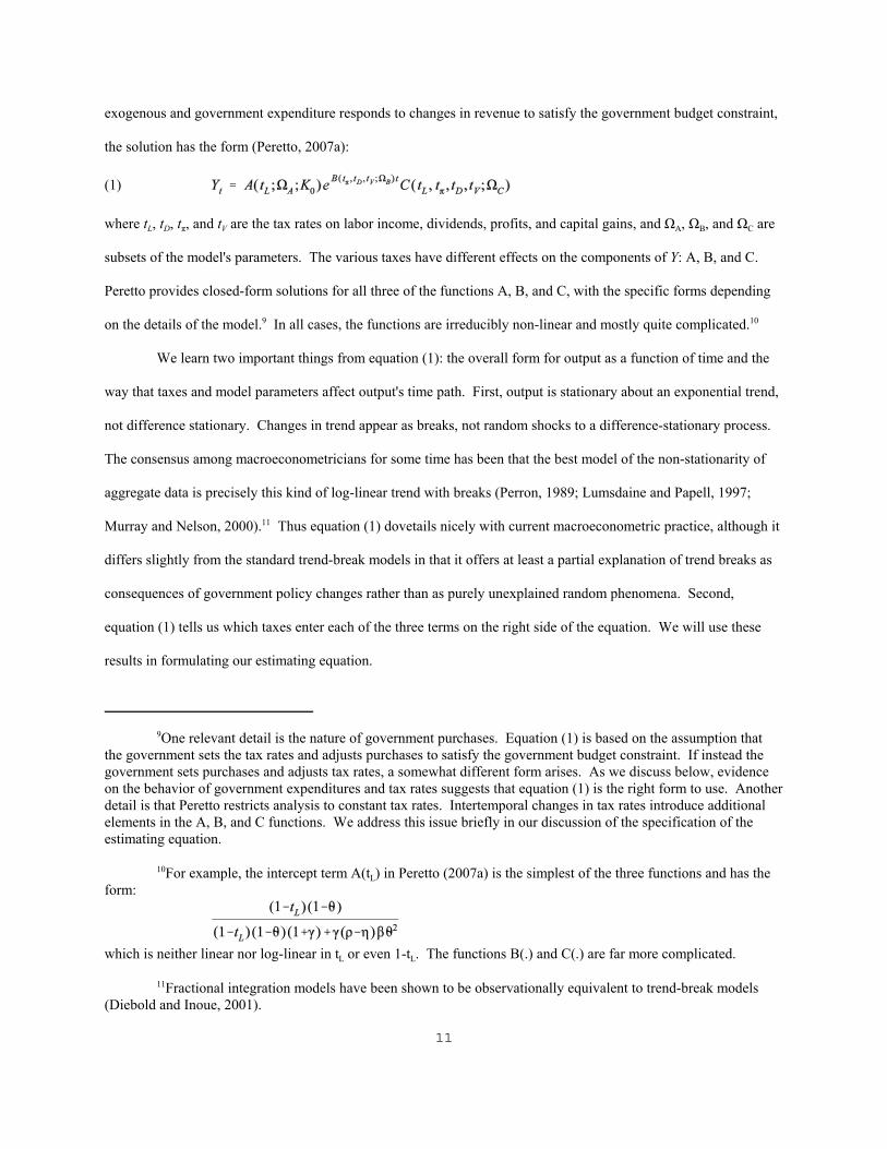
exogenous and government expenditure responds to changes in revenue to satisfy the government budget constraint,

the solution has the form (Peretto, 2007a):

(1)

where tL, tD, tπ, and tV are the tax rates on labor income, dividends, profits, and capital gains, and ΩA, ΩB, and ΩC are

subsets of the model's parameters. The various taxes have different effects on the components of Y: A, B, and C.

Peretto provides closed-form solutions for all three of the functions A, B, and C, with the specific forms depending

on the details of the model.9 In all cases, the functions are irreducibly non-linear and mostly quite complicated.10

We learn two important things from equation (1): the overall form for output as a function of time and the

way that taxes and model parameters affect output's time path. First, output is stationary about an exponential trend,

not difference stationary. Changes in trend appear as breaks, not random shocks to a difference-stationary process.

The consensus among macroeconometricians for some time has been that the best model of the non-stationarity of

aggregate data is precisely this kind of log-linear trend with breaks (Perron, 1989; Lumsdaine and Papell, 1997;

Murray and Nelson, 2000).11 Thus equation (1) dovetails nicely with current macroeconometric practice, although it

differs slightly from the standard trend-break models in that it offers at least a partial explanation of trend breaks as

consequences of government policy changes rather than as purely unexplained random phenomena. Second,

equation (1) tells us which taxes enter each of the three terms on the right side of the equation. We will use these

results in formulating our estimating equation.

9One relevant detail is the nature of government purchases. Equation (1) is based on the assumption thatthe government sets the tax rates and adjusts purchases to satisfy the government budget constraint. If instead thegovernment sets purchases and adjusts tax rates, a somewhat different form arises. As we discuss below, evidenceon the behavior of government expenditures and tax rates suggests that equation (1) is the right form to use. Anotherdetail is that Peretto restricts analysis to constant tax rates. Intertemporal changes in tax rates introduce additionalelements in the A, B, and C functions. We address this issue briefly in our discussion of the specification of theestimating equation.

10For example, the intercept term A(tL) in Peretto (2007a) is the simplest of the three functions and has theform:

which is neither linear nor log-linear in tL or even 1-tL. The functions B(.) and C(.) are far more complicated.

11Fractional integration models have been shown to be observationally equivalent to trend-break models(Diebold and Inoue, 2001).

11

Taxes alter various net rates of return and so appear in Peretto’s models as modifications of some of the

underlying parameters. Regulation also alters net rates of return and so has effects similar to taxes. As with taxes,

exactly how regulation enters the analysis depends on the specific regulation, but in general regulation may modify

every parameter in an macroeconomic model. Various regulations certainly affect total factor productivity in the

production of final goods (e.g., Title 7: Agriculture; Title 12: Banks and Banking; Title 15: Commerce and Foreign

Trade; Title 30: Mineral Resources; Title 49: Transportation), the degree to which quality improvement raises

productivity (e.g., Title 37: Patents, Trademarks, and Copyrights), entry costs (e.g., Title 16: Commercial Practices),

and fixed cost (e.g., Title 20: Employees’ Benefits; Title 29: Labor; Title 38: Pensions, Bonuses, and Veterans’

Benefits). Regulations may affect both the population growth rate and the rate of time preference by affecting the

probability of dying (e.g., Title 21: Food and Drugs; Title 42: Public Health).12 Finally, regulation (e.g., Title 16:

Commercial Practices) may even affect the preference for leisure relative to consumption by affecting advertising,

which in turn can alter tastes, as discussed by Sa (2007). We thus can expect regulation to enter the equation for

output in each place that one of the underlying parameters enters. Ideally, we would enter different kinds of

regulations in various parts of the equation, just as Peretto did with taxes, but data limitations make the ideal

infeasible. The CFR organizes regulations by broad categories called titles. Different regulations within the same

title may do very different things. For example, some regulations in Title 29 (Labor) deal with job safety, and others

deal with collective bargaining. We have page counts for each CFR title but not for lower levels. We thus cannot

distinguish among regulations that may be very different and so are limited to including only our overall measure of

regulation as follows:

(2)

where Rt is our measure of regulation. Regulation has three distinct types of effects: (i) level effects through the

intercept term A(.), (ii) growth rate (or trend) effects through the exponent B(.), and (iii) transition dynamic effects

through the term C(.). We will estimate a version of equation (2) so that we can measure these three effects.

12The probability of dying affects the rate of time preference in the household choice model extended toinclude random time of death. See Blanchard (1985).

12

4. Estimation

We begin our empirical investigation with a discussion of the variables to be examined and then turn to the

econometric analysis.

4.1. Variables To Be Examined

We want to study the effect that federal regulation has on macroeconomic activity. As noted earlier,

regulation grows most of the time, but there is great variation in the growth rate. That variation allows us to perform

tests of the relation between regulation and the other variables. The obvious macroeconomic variable to examine is

real aggregate output, and indeed that is the focus of our study. However, regulation presumably affects the

economy in complex ways, so we also examine how regulation affects the main determinants of output. If we

suppose a Cobb-Douglas production function, then output Yt is given by

where Dt is total factor productivity (hereafter, TFP), Kt is capital services, and Nt is labor services. In what follows,

we examine how regulation affects D, K, and N as well as Y.

4.2. Data

Regulatory activity (R) is the total page count of the CFR, discussed above. Real output in the private

business sector (Y), private capital service flows (K), and hours of labor services (N) are from the Monthly Labor

Review. Output (Y) is real output in the private business sector, which is gross domestic product less output

produced by the government, private households, and non-profit institutions. Capital (K) is service flows of

equipment, structures, inventories, and land, computed as a Tornqvist aggregate of capital stocks using rental prices

as weights. Labor (N) is hours worked by all persons in the private business sector, computed as a Tornqvist

aggregate of hours of all persons using hourly compensation as weights. TFP is the Solow residual from a Cobb-

Douglas production function assuming a capital share of thirty percent. We include two explanatory variables other

than regulation: total government purchases (G) and the federal marginal tax rate on personal income (T).

Government purchases is the sum of government consumption and government investment and is from NIPA. The

marginal tax rate is from Stephenson (1998) with updates to 2005 computed by us. It includes both the federal

13

personal income tax and the Social Security tax.13 Although theory suggests different roles for different taxes, as

shown in equation (2), data are not available for separate marginal tax rates on labor income, corporate profits,

dividends, or capital gains. The main taxes on labor income are the personal income tax and the Social Security tax.

Corporate profits are taxed twice, once by the corporate income tax and once by the personal income tax. The

marginal corporate income tax is notoriously difficult to measure because almost-whimsical tax provisions that come

and go over time, such as safe harbor leasing in the 1980s, have huge effects on the effective tax rate. Dividends are

taxed at the personal income tax rate, but capital gains sometimes are taxed that way and sometimes are taxed under

special provisions. All in all, Stephenson's measure of the effective marginal income tax rate seems a reasonable

proxy for “the” tax rate. We thus replace the four separate tax rates tL, tπ, tD, and tV in equation (2) by Stephenson's

single rate and modify the estimation equation accordingly, as discussed below. Figures 3 and 4 show the time

series for G and T. All data are annual observations for the U.S. over the period 1949-2005.

Finally, Figures 1-4, and indeed all the rest of our figures, show both the raw data and the H-P filtered data,

but all the analysis that follows uses the raw data only. The H-P filtered data are shown solely to illustrate the

general movements of the data, which often are obscured by the high-frequency variation of the raw series. Also,

some figures show levels and others show growth rates, whereas our empirical work uses a mixture of levels and

log-levels, as discussed below.

4.3 Regression Model and Estimation Issues

We explain how we use equation (2) to obtain a tractable estimating equation. We then discuss the

stationarity properties of the data and the exogeneity of our explanatory variables.

4.3.A. The Regression Model. Equation (2) gives us a general form for our estimation equation. Peretto (2007a)

derives closed-form solutions for the three functions A(.), B(.), and C(.) in his equation (1) because he has a

completely specified function for each tax law; in particular, each tax is linear and constant over time. We cannot

obtain closed-form solutions for A(.), B(.), and C(.) because we do not have specific functional forms for the way

regulation affects the economic quantities. We therefore use quadratic approximations for A(.), B(.), and C(.). Also,

13Barro and Ridlick (2011) present an alternative series on marginal income tax rates. It is an extension ofthe series originally published by Barro and Sahasakul (1983, 1986). However, Akhand and Liu (2002) have shownthat the Barro-Sahaskul construct is considerably inferior to Stephenson’s as a measure of average marginal taxrates, so we restrict attention to Stephenson’s series.

14

regulation is not constant but changes over time, so we generalize equation (2) by including lagged as well as current

regulation to pick up the extra transition dynamics induced by time-varying regulation. The quadratic is simple and

suffices for this first empirical exploration of regulation’s macroeconomic effects. It has some undesirable

implications for extrapolation beyond the sample period, as we discuss below, so further research on functional

forms for the trend coefficient would be useful.

We thus have

(3)

where X is any of our dependent macro variables Y, TFP, K, or N; Z is an exogenous explanatory variable for X (such

as R, T, or G); α, β, γj, δj, and ωj are constants; Ji are lag lengths; and U is a log-normally distributed residual.

Generalization to the case where Z is a vector is straightforward. The entire first term in parentheses in equation (3)

is a trend term. The trend coefficient is a quadratic function of Z. It nests the simpler linearly detrended model with

constant trend (γi = 0, δj = 0 for all I, j). The second large term in parentheses in (3) is a combination of the intercept

and cycle terms A(.) and C(.) in equation (2) that we explain in more detail presently.

We base our estimation on equation (3). It is not quite in the same form as equation (2), the growth

equation that motivates it, because Z may contain a trend of its own. Equation (2) collects all trend elements in the

single term B(.). It is easy to see, however, that equations (2) and (3) are equivalent by decomposing Z into its trend

and cycle components and then combining the trend component with the first term in parentheses in (3) to obtain a

total trend term. Suppose Z obeys

where αZ and βZ are constants, with βZ being the trend in Z, and V is a log-normally distributed residual that is the

variation about the trend. Substituting into (3) and doing some straightforward algebra gives

(4)

15

where A = exp(α+αZΣω-βZΣjωj) and C = (ΠVt-j.ω)Ut. Equation (4) has the same form as equation (2).

The first term A in equation (4) is a constant, the second term is the trend with trend coefficient B(Zt) = β +

βZ Σωj + Σγj Zt-j + Σδj Zt-j2, and the third term C is the compound residual U(ΠVω). The first term inside B(Zt) is the

constant β, which captures trend elements apart from any effects of Z. In particular, it would be the trend in X if Z

were held constant, a fact we use in the analysis below. The last three terms in B(Zt) collect the various effects of Z

on the trend in X. In what follows, we refer to the first term β as the trend-apart effect (because it captures the trend

that would be present if all the exogenous variables were trendless), the second term βZΣωj as the trend-intercept

effect of Z, the third term as the trend-linear effect, and the fourth term as the trend-quadratic effect. The trend-

intercept effect is constant. Below, we discuss counterfactual paths that would have emerged if exogenous variables

had been held constant. Doing that requires distinguishing among the quantities β, ωβZ, and β+ωβZ. The compound

residual U(ΠVω) is the cycle term and corresponds to C(.) in equation (2). If X is either individually stationary or

jointly trending (cointegrated) with Z, the compound residual is purely transient, causing fluctuations about trend.

The term ΠVω captures the part of the residual due to Z's deviation from its trend. We call this transient component

the cycle effect.14 When Z equals its “normal” (or balanced growth) value, there is no transient effect, Vt-j = 1 for all

j, and the only remaining level effect arises from the intercept term .

Transition dynamics appear in two places in equation (3) or (4): the lagged values of the explanatory

variables included in the growth rate and the lagged values included in the cycle effect. The balanced growth rate is

the value of the growth rate in (3) or (4) when Z is constant. When Z changes, the balanced growth rate also

changes, causing transition dynamics in going from the old balanced growth path to the new one. Changes in Z

induce additional transition dynamics through the cycle effect. The cycle effect captures movements about a given

growth path. The same type of distinction appears in discrete-time ARIMA models in which a variable's level has a

growth term and a random term, and the growth term itself is stochastic with a random term, such as

Both ut and vt cause transition dynamics. The growth term that appears in the transition dynamics here was absent

14The U component of the compound residual can include any exogenous variable not subject to analysis. The trends in such variables are included in the trend-apart term β, so that U captures the transient components.

16

from equation (2). It arises from time variation in the regulation and tax parameters which were treated as constant

in equation (2). Peretto (2007a) restricted his analysis to an economy that starts off the balanced growth path (and

therefore has transition dynamics) but that has constant values for all policy parameters. In contrast, we must allow

changes in the policy parameters to capture the intertemporal variation present in the data.

To carry out the estimation, we take natural logs of both sides of (3) to obtain

(5)

where lower-case variables are the natural logs of corresponding upper-case variables.

4.3.B. Stationarity Properties of the Variables. Equations (3) and (5), derived from economic theory, suggest that

output may be trend-stationary. Is it? If so, we can estimate equation (5) as is. If not, we must reconsider the

appropriate econometric method for estimating the equation. We test the natural log of output for a unit root in both

the absence and presence of structural breaks. We use natural logs because those are the forms in the estimating

equation (5). Table 3 reports the test results. The DF-GLS (Elliott, Rothenberg, and Stock, 1996) test cannot reject

a unit root in the natural log of output at the 5% level. However, it is well known that conventional unit-root tests

often fail to reject the unit-root null when there is a break in the trend function under the stationary alternative

hypothesis.15 Thus, we consider the unit-root test proposed by Zivot and Andrews (1992) which allows for structural

breaks. The Zivot-Andrews test also fails to reject the unit-root null. These results suggest that output’s time series

behavior is nonstationary. The DF-GLS and Zivot-Andrews tests also fail to reject a unit root for TFP, physical

capital, and labor–the other dependent variables considered in our analysis.

We also conduct stationarity tests for the independent variables in our model–namely, regulation, the

marginal tax rate, and government purchases. These results are also reported in Table 3. The DF-GLS and Zivot-

Andrews tests fail to reject the unit-root null for regulation, suggesting that it is nonstationary. For the marginal tax

rate, the Zivot-Andrews test provides a rejection at the 5% level of significance, but not the 1% level. In light of this

marginal rejection, we will proceed in the analysis that follows with the assumption that the marginal tax rate is also

nonstationary. The Zivot-Andrews test provides a strong rejection of the unit-root null for government purchases,

clearly suggesting that it is a stationary variable.

15See, for example, Perron (1989, 1997), Banerjee et al. (1992), Zivot and Andrews (1992), and Vogelsangand Perron (1998) for further details.

17

Taken together, the results in Table 3 suggest that the variables in our model are nonstationary. (The only

exception is government purchases, whose inclusion in the model will be addressed further in the following section.)

A finding that all of the variables in the model are nonstationary suggests that a cointegrating relationship is the only

possibility that is consistent with our theory. To test for cointegration, we conduct Engle-Granger cointegration tests

for each of our dependent macro variables (individually) and the independent variables (jointly, excluding

government purchases) in our model. The null hypothesis of no cointegration is rejected at conventional

significance levels in the test for cointegration among output and the independent variables. However, the tests for

total factor productivity, physical capital, and labor fail to reject the null hypothesis. It is well known that the power

of these tests is low (see Hakkio and Rush, 1991) and we do not want to throw out a well-formulated theory on the

basis of low-power econometric tests. An alternative test for cointegration is the Johansen test. The Johansen

methodology, however, also seems inappropriate since it generally produces a vector error correction model which is

inconsistent with our theory which suggests estimating the model in levels. As such, we will proceed with the

estimation of the model suggested in equation (5) using single-equation methods that correct the standard errors for

the presence of cointegrated variables. We defer further discussion of the appropriate estimation technique to the

following sections.

4.3.C. Exogeneity. We also need to examine the sensitivity of our endogenous macro variables to the three policy

variables: regulation R, government purchases G, and the marginal tax rate T.16 Granger-causality tests for R and the

dependent variables we want to consider (output Y, total factor productivity TFP, physical capital K, and labor N) are

reported in Table 4. We conduct the tests using natural logs of all variables x = lnX to be consistent with our

estimating equation (5).17 At the 10% significance level, there is causality running from r to tfp, k, and n, and no

causality running from any of the dependent variables to r, a finding that is consistent with econometric exogeneity

of r. We also perform Granger-causality tests (not reported in Table 4) of the exogeneity of g and τ = lnT. The tests

16We have not pursued the possibility of decomposing G into major parts (such as federal versus state andlocal, or national defense versus road building), even though different kinds of expenditure almost certainly havedifferent effects on the economy and may interact with regulation in different ways. We also ignore governmentdebt on the assumption that Ricardian equivalence holds, a proposition with much support in the empirical literature.

17Both log-levels and levels of R, T, and G appear in (5), so we examined Granger causality using levels ofR, T, and G as well. The results are qualitatively the same as those reported in Table 4.

18

indicate econometric exogeneity of τ, but g appears to be econometrically endogenous, with causality never running

from g to the dependent variables but running from both y and τ to g. These results are consistent with government

setting tax rates and then choosing G to satisfy the government budget constraint as tax revenue fluctuates with the

movement of the economy. In light of these results, we treat R and T as exogenous and exclude G from the analysis

that follows. Exploration of regressions that include G show no important differences from regressions that omit it,

so henceforth we ignore G. Eliminating G from the analysis also excludes the only variable that is found to strongly

reject the unit-root null in the Zivot-Andrews test reported in Table 3, thus ensuring a cointegrated system.18

4.4. Estimation

When we replace Z by the vector (R,T) in equation (5), we obtain the following estimating equation:

(6)

Note that equation (6) derives from a coherent theory of endogenous growth. It contains no lagged dependent

variables because the underlying theory does not predict the presence of such variables, as shown in equation (2). It

also is not a VAR. VARs usually can be considered as linear approximations to a poorly understood theoretical

model, useful when the theory provides little guidance on the correct specification. In contrast, we have a well-

developed theory providing a great deal of information on the equation to be estimated, which does not include a

lagged dependent variable.

In light of the stationarity properties of our variables discussed above, we need an appropriate methodology

for estimating equation (6). We use the dynamic OLS (DOLS) procedure suggested by Saikkonen (1992) and Stock

and Watson (1993). The DOLS method involves augmenting equation (6) with p lags and q leads of ΔZt, which

eliminates the feedback in the cointegrating system and produces an asymptotically efficient estimator. More

specifically, for Z given by the vector (R,T) the DOLS procedure adds

to the model to be estimated in equation (6). Standard OLS estimates of the coefficients from the augmented

18We also performed Granger-causality tests on the individual titles of the CFR. Few individual titlesGranger-cause any of the macroeconomic variables considered here, but the whole set of titles is jointly significant. With nearly 50 individual titles and only 57 observations, the tests have few degrees of freedom, leaving the resultsuninformative. This problem with degrees of freedom arises again later, where we discuss it in more detail.

19

regression are consistent, but the usual t- and F-statistics must be re-scaled using an estimate of the long-run

variance of the DOLS residuals. See Hamilton (1994, 608-612) for a description of this non-parametric correction

for serial correlation. The coefficient estimates on the lags and leads of ΔZt are of no interest and are not reported.

In the DOLS estimation of (6), the lag lengths Jx and the appropriate number of lags p and leads q of ΔZt are

chosen by imposing an initial value of 3 on Jx and 5 on p and q and searching, subject to two restrictions, over all

possible smaller values to find that which minimizes the Schwarz-Bayes Criterion (SBC). The restrictions on the

search procedure were (1) the constant always was retained and (2) no variable could be omitted unless all of its

more-lagged values also were omitted. For example, even if the lowest SBC value was obtained with a model that

excluded Zt but retained Zt-1, that model was not considered. Exclusion of Zt would be allowed only if Zt-1 also was

excluded. The reason for that restriction was that, with annual data, it did not seem reasonable to suppose that a

variable could have an effect only with a one-period lag. Table 5 reports the estimation results for the four macro

variables of interest. Part I of the table shows the estimated values for all coefficients pertaining to regulation and

Part II shows all other parameter estimates. Very few lagged variables are significant, so to save space Table 5 is

restricted to those lags that had significant coefficients in at least one equation.

Regulation has significant effects on all four dependent macro variables, entering with both trend and cycle

terms. In some cases regulation enters with lags, indicating dynamic responses in the dependent variables. Also, the

coefficient patterns and magnitudes differ across dependent variables, indicating compositional effects. As we have

seen above, regulation can have two kinds of effects on a dependent variable’s trend: a shift in the trend (the trend-

intercept effect) and breaks in trend (the trend-linear and trend-quadratic effects). Our results indicate that both

kinds of effects are present. The trend-intercept effect is the product of regulation’s trend βR and the sum of the ωjR

coefficients. The latter are reported in Table 5 and the former is obtained by estimating the equation rt = αR + βRt +

νt. The estimated value of βR is 0.0322. Estimating the analogous equation for the tax rate gives a trend in T of βT =

0.0058.

4.4.A. Output. For output, there are two ωjR coefficients, which sum to -1.210. Its product with βR is -0.039,

indicating that regulation shifts the trend in output down by 3.9 percentage points. That shift, being a reduction in

the intercept of the trend coefficient function B(Rt), is uniform over time. In addition, regulation has time-varying

effects on output's trend through the trend-linear and trend-quadratic terms of the coefficient function B(Rt). The

20

sum of trend-linear coefficients is positive, causing output’s trend to rise on net as regulation grows, and the trend-

quadratic coefficient is negative, indicating that the trend-quadratic effect is negative and causes output's trend to fall

as regulation grows. We thus have a non-linear effect of regulation on output’s trend. Figure 5 shows the total

effects of regulation on output’s trend over time. The effect is always negative but is nonlinear. Growth in

regulation raises output’s trend (that is, makes it less negative) until about 1980 and then reduces it. The effect is

actually positive from the mid-1970s through the mid-1990s. The average value of the negative effect on output's

trend is -0.0195, or nearly two percentage points.

The reduction in trend is not the total effect of regulation on output. The large negative values of ω0R and

ω1R indicate that regulation also has a substantial cycle effect on output. We can determine regulation's total effect

by using the parameter estimates and regulation data to calculate a counterfactual value of output that would have

obtained had regulation stayed at its 1949 level.19 Figure 6 plots the ratio of actual Y to counterfactual Y. The time

pattern is irregular. The ratio first falls until about 1960, then remains nearly constant until about 1970, then falls

again before leveling off in the early 1980s, falls sharply from the mid-1980s through the mid-1990s, rises in the late

1990s, and then falls sharply through 2005. Overall, the ratio falls over the sample period indicating that

regulation's total effect on output has been negative.

The overall decline in output relative to its counterfactual is large. By the end of the sample period, output

is down to 28 percent of its counterfactual, reflecting principally the compounding of the reduction in output’s trend

growth rate and secondarily the accumulation of cycle effects over a period of 57 years. Using the formula 0.28 =

eβ*57, where β* is the realized average reduction in output's growth rate and 57 is the number of years in the sample,

we can calculate that β*.-0.022, or just over two percentage points. As noted above, the average reduction in

output’s trend is about 0.0195. The discrepancy reflects the fact that the regulation-induced reduction in output’s

trend is not constant but rather varies over time, as shown in Figure 5, and it interacts with the time-varying cyclical

19More specifically, in the trend term we replace Rt with (Rt-R1949)+R1949 / ΔRt+Rt and replace Rt2 with [(Rt-

R1949)+R1949]2 = (ΔRt)

2+2RtΔRt+(Rt)2, multiply by the appropriate estimated trend coefficients (γ and δ), and collect all

terms containing ΔRt. Similarly, in the cycle term we replace Rt with R1949(Rt/R1949), raise to appropriate estimatedpower (ω), and collect all terms involving ratios of the form (Rt/R1949)

ω. Finally, dividing actual output by the trendarising from the terms containing ΔRt and by the cycle components (Rt/R1949)

ω is equivalent to setting ΔR to zero and(Rt/R1949)

ω to one, thus giving a counterfactual value of output under the restriction that regulation remained at its1949 level.

21

effects.

We can convert the reduction in output caused by regulation to more tangible terms by computing the dollar

value of the loss involved. The sample period ends in 2005, but let us assume that the same final ratio of 0.28

applies today. In 2011, nominal GDP was $15.1 trillion. Had regulation remained at its 1949 level, current GDP

would have been about $53.9 trillion, an increase of $38.8 trillion. With about 140 million households and 300

million people, an annual loss of $38.8 trillion converts to about $277,100 per household and $129,300 per person.

Furthermore, our estimates indicate that the opportunity cost will grow at a rate of about 2 percent a year (the

average reduction in trend over the sample period) if regulation is merely kept at its 2005 level and not increased

further.20

Four aspects of the output opportunity cost are noteworthy. First, our figures are net costs. They are based

on the change in total product caused by regulation and so include positive as well as negative effects. Our results

thus indicate that whatever positive effects regulation may have on measured output are outweighed by the negative

effects. Second, our measure does not include any non-production benefits of regulation. The non-production

benefits could be both large and growing. Pollution, for example, presumably grows as unregulated industrialization

expands and the costs of pollution presumably are convex in the amount of pollution. Any such costs have been

reduced by environmental regulation. If regulation has reduced the growth rate of pollution, not just its level, then it

correspondingly has introduced a growing benefit that is not included in measured output. We do not attempt to

measure such benefits here, confining our analysis strictly to measured output. Consequently, we emphasize that our

results offer no conclusion on whether regulation is a net social benefit.21 They do, however, make clear that the cost

of regulation is substantial and must be taken seriously in any evaluation of regulation’s net social benefit. Third,

our estimated opportunity cost pertains only to regulation added since 1949. We have no way to measure the

20Of course, because we have restricted our functional form to a quadratic, ridiculous results can beobtained by extrapolating far beyond the sample period. If regulation continues to grow, the negative terms takeover and eventually output growth becomes negative, driving output toward zero as time passes. Such behaviorobviously would not be tolerated by society, and the process governing the evolution of regulation would change. The problem is exactly the same as using a quadratic utility function to approximate the true function: it can workquite well locally but will give nonsensical results if abused. These problems of extrapolation are not relevant to ourdiscussion here, which is confined to behavior within the sample period.

21Indeed, Peretto (2008) finds that changes in tax rates can reduce the growth rate of output but raise socialwelfare. The same divergence could happen with regulation.

22

opportunity cost associated with regulation up to 1949. It seems certain that some regulation has a negative

opportunity cost, that is, a net positive effect on GDP. Surely GDP would be lower in the absence of traffic

regulations, for example. However, most of those most basic regulations were in place well before 1949, so for our

work their benefits are simply a given that is impounded in the intercept. Fourth, regulation's opportunity cost is far

larger than its compliance costs, a topic studied in the existing literature. For example, Crain and Hopkins (2001)

estimate the compliance cost of all federal regulation (not just post-1949 regulation) to be about 8 percent of current

GDP, or about $1.2 trillion in mid-2011.22 Our estimates of regulation's opportunity cost arising from reduced GDP

are approximately 32 times larger than the compliance cost.

4.4.B. Comparison with Previous Estimates of Regulation's Growth Effects. Our estimates of the output losses

induced by regulation may elicit “sticker shock” on the part of the reader. Partly that is the nature of exponential

growth. Even experts used to working with growth rates often substantially underestimate the effects of even small

changes in growth rates on the corresponding levels (Christandl and Fetchenhauer, 2009). However, there also is a

legitimate concern that such large effects should be checked to make sure they are not an artifact of something. We

therefore turn to a comparison of our estimates of regulation's growth effects with estimates already in the literature.

Our estimates are consistent with previous estimates obtained from both aggregate and disaggregate data. In fact,

our estimates are on the low side compared to many previous results.

Consider first the aggregate data. Maddison (2000) reports (Table B-22) that country growth rates around

the world varied tremendously over the period 1950-1998. The highest rates were in Japan (5.20%), the rest of Asia

(3.23%), and Western Europe (2.93%), and the lowest rates were in the former USSR (0.81%) and Africa (1.04%).

Parente and Prescott (1999) argue that most of the differences between the high and low growth rates were the result

of “barriers to riches” erected principally by various forms of regulation.23 The difference between Maddison's

maximal and minimal growth rates is 4.39% or 0.0439. Our estimate of 0.02 for regulation's impact on the US

growth rate is quite modest by comparison.

22This 8 percent excludes the cost of tax compliance, which Crain and Hopkins included. We exclude taxcompliance cost because taxes generally are not considered “regulations.” Tax compliance cost amounts to aboutone half of one percent of GDP.

23See especially Parente and Prescott's chapters 6 and 7.

23

Several studies mentioned earlier use the cross-section data on regulation to examine the impact of specific

types of regulation on aggregate growth. Loayza, Oviedo, and Sevren (2004) examine seven main areas of a firm's

activity subject to regulation: entry, exit, labor markets, fiscal burden, international trade, financial markets, and

contract enforcement. For each area, they construct an index of the severity of regulation and also an overall index

for the seven areas taken together (the index comprises a small subset of all regulations, as explained in section 2.4

above). They find that increasing a country's index of regulation by one standard deviation (i.e., by 34%) would

decrease its annual rate of per capita GDP growth by 0.4 percentage points. By comparison, our time-series study of

the US indicates that an increase in total regulation of 600% reduces growth by just 2 percentage points. Relatively

speaking, our effect is smaller. Also, Loayza et al. find that decreasing product market regulation in a typical

developing country to the median level of industrial countries (that is, from 0.51 to 0.17, which is a reduction of

67%) would raise that country's annual growth rate by about 1.3 percentage points, a magnitude that is completely

consistent with Parente and Prescott's (1999) argument that regulation is a major cause of income differences. It is

also in line with our result for changing total regulation in the US.

Djankov et al. (2006) study regulations that help or hinder business performance in 135 countries and in

several regulatory areas: starting a business, hiring and firing workers, registering property, getting bank credit,

protecting equity investors, enforcing contracts in the courts, and closing a business. They find very large effects on

growth:

"The impact of improving regulations is large. In Table 3, we analyze the magnitude by including

dummies for each quartile of the business regulation index in the OLS regressions. Improving

from the worst (first) to the best (fourth) quartile of business regulations implies a 2.3 percentage

point increase in average annual growth [rate of GDP per capita]." (p. 400)24

All of these results, many of which only apply to subsets of regulations, are similar to or larger than what we obtain

with time series data for total regulation in the US. By comparison, then, our result is not incredibly large.25

24Note that there is a misprint in Djankov et al.’s published Table 3. The entry in the first row of the lastcolumn of Table 3 should be -2.3241, not -.3241. See their earlier working paper (2005) for the correct entry.

25Other estimated aggregate effects of regulation also are large. For example, Loayza, Oviedo, and Sevren(2005) find that increasing a country's index of labor regulation by one standard deviation in the cross-countrysample would increase the size of the informal sector relative to GDP by nearly 3 percentage points. Nicoletti et al.

24

One may wonder if perhaps the large growth effects are somehow an artifact of aggregate data. It therefore

is useful to look at estimates of regulation's effects obtained from disaggregate data. Such studies cannot, of course,

estimate aggregate growth effects, but they can tell us whether regulation's effects at the micro level are large or

small. If they are small, then one has reason to be skeptical of the large effects found at the aggregate level. In fact,

the effects at the micro level are quite large.

Several studies use the OECD series on regulation discussed above to examine the effect of regulation at

the micro level. Nicoletti et al. (2001), using industry level data in OECD countries, find that employment

protection and product market regulations have large and statistically significant effects on market structure and

R&D expenditure. The employment share of large enterprises (a measure of industrial structure) has an average

elasticity across countries and industries with respect to employment protection regulation of about -1.5 in

manufacturing and -1.0 in non-manufacturing (see their Table 2).26 Manufacturing R&D expenditure has an

elasticity with respect to employment protection regulation of about -0.6 (see their Table 6). Nicoletti and Scarpetta

(2003) study the effects of product market regulations for detailed manufacturing and service industries in the OECD

countries. They find that countries with an above-average share of state-owned firms (such as Finland, France, and

Italy, among others) would increase transitional multifactor productivity growth by about 0.7 percentage point and

steady-state growth in the manufacturing sector by 0.2-0.4 percentage point simply by reducing the state-owned

share to the OECD average (p.40). Bassanini and Ernst (2002) find that the elasticity of R&D intensity (R&D

expenditures relative to the value of output) in 2-digit manufacturing industries of the OECD countries has an

elasticity with respect to employment protection regulation of about -1.0 (see their Table 3). Alesina et al. (2003)

study the relation between regulation and investment in the transport (airlines, road freight and railways),

communication (telecommunications and postal) and utilities (electricity and gas) sectors. Their cross-country

estimates imply that decreasing regulation by 40% raises investment in those sectors by about 2.5 percentage points.

(2001) find that cross-country differences in product market regulations in the OECD account for up to 3 percentagepoints of deviations of the employment rate from the OECD average.

26Nicoletti et al. report (in their Table 2) a semi-elasticity of -0.75. We converted that to an elasticity usingthe average product market regulation value of 1.94, found by averaging the individual country values reported inNicoletti, Scarpetta, and Boyaud (2000), Table A3.6. We made similar conversions for semi-elasticity estimatespertaining to employment protection regulation, using the average value of employment protection regulation fromTable A3.11 in Nicoletti et a. (2000).

25

An estimate of the effect of regulatory reform in the UK over several years starting in 1984 yields an elasticity of

communication and transport investment with respect to their index of regulation of -0.77. The OECD (2003), using

firm-level data, finds an elasticity of new firm entry rates with respect to product market regulations of about -3.0

(see their Table 4.6, column D).27 All of these estimated effects of regulation are quite large and show that the large

effects at the aggregate level are consistent with what is seen at the micro level.

The foregoing studies all use some type of cross-section data on subsets of regulation, whereas our

estimates are based on time series data on the total body of US regulation. Our estimates of regulation's effects

typically are lower than those from the cross-section data. There may be a systematic difference between time series

data on the one hand and cross-section and panel data on the other, or it may be that many of the regulations

included in our comprehensive measure that are omitted from the OECD measure have smaller effects than the

subset of regulations included in the OECD measure, thus leading to a smaller average effect, or our page-count

series may have more measurement error that the OECD survey measure, diluting the measured impact of regulation

that we obtain from our measure. The source of the difference deserves further study. In any case, though, the

comparison of our estimates with those obtained from alternative series using both macro and micro evidence does

suggest that the large effects we report above are by no means implausibly large.

One difference between our results and those of most of the existing literature is that we include the

marginal tax rate T as an explanatory variable. We explored the effect of omitting T. Qualitatively, the results were

unchanged, but quantitatively the omission of T made a difference. The effects of R on Y and TFP is larger when T

was omitted than when it is included, though they still are smaller than what most of the micro-based literature finds.

Thus part but not all of the difference between our estimated effects and those of the micro-based literature seems to

reflect an omitted variable problem in the latter.28

4.4.C. TFP and the Productivity Slowdown. Figures 7 and 8 plot the growth rates of output and TFP. It is easy to

see from the Hodrick-Prescott filtered series that the two variables move closely together with closely matched

27The OECD's (2003) regressions for entry rates are in levels, so the estimated coefficients are simplederivatives: d(entry rate)/d(regulation). We converted to elasticities by multiplying by (regulation)/(average entryrate . 0.10), where the country entry rates are reported in Nicoletti et al. (2001), Table A2.1.

28In this regard, our results differ from those in Alesina et al. (2003), whose estimates of regulatory impactare insensitive to inclusion or omission of fiscal policy variables.

26

turning points. Comparing Figure 8 with Figures 1, 2, and 4 suggests that regulation and taxes had something to do

with TFP’s behavior. TFP growth drops abruptly at the start of the sample, but that seems to be an artifact of the

leverage that the first point in the sample has on the initial part of the Hodrick-Prescott filtered series. If we ignore

that episode, then TFP really starts falling sometime in the mid 1960s, stops falling in the early 1980s, and grows

slowly after that. The falling growth rate between about 1965 and 1980 is the well-known “productivity slowdown.”

The marginal tax rate and the growth rate of regulation began rising at almost exactly the same time as TFP's growth

rate turned down in the mid 1960s. Regulation's growth peaked in the second half of the 1970s, a little before TFP

turned back up, and even became negative in the mid-1990s (see Figure 2). Tax rates peaked at almost exactly the

same time that TFP bottomed out, stopping their rise around 1980 and falling somewhat afterward. Thus, it appears

that major changes in TFP correspond to major changes in R and T.

We can use our parameter estimates to quantify this impressionistic visual analysis. The second column of

Table 5 reports the TFP estimates. Using those in the same way as we did for output, we can calculate the effects of

regulation and taxes on TFP. Figure 9 shows the effect of regulation on TFP’s trend. The effect is negative

throughout the sample period, but increases in regulation actually decrease this negative effect on TFP’s trend

through about 1980. This suggests that, to the extent that regulation contributed to the productivity slowdown, it

must have occurred through cyclical rather than trend effects. The combined trend and cyclical effects of regulation

can be obtained by constructing the counterfactual series which shows the level of TFP had regulation remained at

its 1949 level. Figure 10 shows the change in the ratio of actual TFP to counterfactual TFP. As with output, there is

an initial point artifact. Ignoring that, we see that the change in the ratio is about zero in 1965 and then becomes

increasingly negative until about 1980. After that, the change rises sharply and is positive in some years through the

late 1990s, after which it falls again. Throughout the 1965-1980 period the change is negative, indicating a

persistent negative effect of regulation on TFP during the infamous productivity slowdown.

Taxes may also play a role in explaining TFP growth. Figure 11 plots the change in the ratio of actual TFP

to counterfactual TFP obtained by holding the marginal tax rate at its 1949 level. Although the effect of taxes is far

from constant over time, it is difficult to detect a discernable trend during the years of the productivity slowdown.

Indeed, the HP filtered series is generally flat and close to zero over the entire sample period. Thus, it appears that

the effect of regulation may dominate that of taxes in explaining the productivity slowdown. This conclusion is

27

confirmed in Part II of Table 5, where the sums of the trend-linear and trend-quadratic tax terms in TFP’s trend are

found to be insignificantly different from zero.

Figure 12 shows the combined effects of regulation and taxes on TFP, plotting the change in the ratio of

actual TFP to counterfactual TFP obtained by holding both the level of regulation and the marginal tax rate at their

1949 values. The pattern over time is similar to that shown in Figure 10, again confirming that regulation’s effect is

dominant. Comparing Figures 10 and 12 with Figure 8, which plots the growth rate of TFP over the sample period,

shows a close match in the slopes and turning points, suggesting that regulation explains a great deal of the changes

in TFP's path, including the productivity slowdown.

The foregoing explanation of the productivity slowdown has an important advantage over alternatives in the

literature. Greenwood and Yorukoglu (1997) offer an explanation of the productivity slowdown based on the idea

that the economy underwent severe adjustment difficulties in adapting to the large amount of investment expenditure

on information technology that began in the late 1970s. Nordhaus (2004) suggests that the productivity slowdown

resulted from the OPEC oil shock of the early 1970s. Though both mechanisms may well have had a role to play,

they cannot be the entire story because the productivity slowdown started five to ten years earlier than either the

technology investment or oil shock in the 1970s. In contrast, as we have seen, significant changes in regulation

occurred at the start of the productivity slowdown in the mid-1960s and then again at the slowdown's end around

1980.

It also is interesting that the TFP slowdown apparently was not due to an R&D slowdown and that

regulation seems to have no statistically significant net effect on R&D. We use the real value of private R&D

expenditure reported by the National Science Foundation as our measure of R&D. The growth rate of TFP has a

slightly negative correlation with the growth rate of R&D. Regressing TFP growth on current and two lags of R&D

growth yields an adjusted R2 of -0.04 and p-values for all R&D coefficients over 0.15. The plot of R&D growth

shows that it is negative in much of the first half of the productivity slowdown but positive in all the second half.

Also, there are other periods in the 1980s and 1990s when R&D growth is similarly negative with no TFP

slowdown. There also is no economically significant relation between regulation and R&D. A simple linear

regression of R&D on current and lagged regulation yields insignificant coefficients. If we use the functional form

in equation (6) with ln(R&D) as the dependent variable x, we obtain statistically significant coefficients on both

28

current and lagged values of the linear and quadratic regulation terms in the trend. However, the sums of all linear

coefficients and of all quadratic coefficients are both negative but also insignificantly different from zero, implying

that regulation's effects on R&D growth disappear within three years. Analysis of the counterfactual path of R&D

(i.e., holding regulation at its 1949 level) yields the result that the regulation terms cancel each other out for the most

part, with no economically significant short-term effects even on the level of regulation.

The absence of an effect of total regulation on R&D is consistent with other econometric evidence and also

with the endogenous growth model that underlies our estimation. The OECD (2003), using data on 18

manufacturing industries in 18 OECD countries, finds that most types of regulation (their PMR measure, consisting

of non-tariff barriers to international trade, tariff barriers to international trade, direct state control of economic

activities, and their EPL, consisting of labor market regulations) reduce R&D expenditure, but regulation that erects

barriers to entry (“barriers to entrepreneurship”, which comprises legal limitations on access to markets and

administrative burdens and opacities hampering creation of businesses) have a strong positive effect on R&D

intensity, with an elasticity of about 1.3.29 This pattern is completely consistent with Peretto's theoretical results that

taxes that directly reduce the return to R&D reduce R&D, as one would expect, but taxes that reduce the return to

entry raise the profit of incumbent firms and induce them to increase their R&D. Our total measure of regulation

mixes regulations that directly make R&D less profitable and regulations that reduce the return to entry. We tried to

examine the effects of individual types of regulation on R&D, but data limitations rendered that impossible, as

discussed below.

4.4.D. Capital and Labor. We do not dwell on the results for capital and labor because they are of secondary

interest and are generally of the same character as those for output and TFP. See the last two columns in Table 5. In

particular, regulation has significant effects on both variables, has both growth and cyclical effects, has both linear

and non-linear effects on the growth terms, and enters with lags. The pattern of coefficients for labor is very similar

to the pattern for output, but the pattern for capital is quite different from those for all the other dependent variables.

The different patterns across the three inputs means that changes in regulation causes shifts in the relative amounts

of inputs used to produce a given amount of output. Regulation affects not only output's path but also the way

29See the OECD's (2003) Table 3.3 for estimated coefficients and see Nicoletti, Scarpetta, and Boylaud(2000), Table A3.2, for values of barriers to entrepreneurship.

29

output is produced.

4.4.E. Individual Titles of the CFR. We tried to isolate the CFR titles with significant impacts on our aggregate

dependent variables.30 However, the large number of titles leaves us too few degrees of freedom to obtain useful

results. We could not include any lags. For each possible dependent variable, a small subset of the titles had

coefficients individually significant at the 10 percent level or less. However, a joint test of the remaining titles

always strongly rejected the null that the remaining titles were jointly insignificant, implying that at least some of the

individually insignificant titles are in fact significant. We thus could exclude no individual title and so could not

identify which individual titles were significant for any dependent variable.

5. Conclusion

We have presented a new time series measuring the extent of federal regulation in the United States, and we

have used it to examine the effect of regulation on the macro dynamics of several aggregate variables of interest.

We find that post-1949 regulation has statistically and economically significant effects on the time paths of output,

total factor productivity, labor, and physical capital. Regulation alters both trends and movements about the trends.

The trend effects usually are complex and non-linear. The cycle effects have lag lengths and coefficient sign

patterns that differ across the dependent variables. Regulation has allocative effects, changing the mix of factors

used to produce output.

Regulation’s overall effect on output’s growth rate is negative and substantial. Federal regulations added

over the past fifty years have reduced real output growth by about two percentage points on average over the period

1949-2005. That reduction in the growth rate has led to an accumulated reduction in GDP of about $38.8 trillion as

of the end of 2011. That is, GDP at the end of 2011 would have been $53.9 trillion instead of $15.1 trillion if

regulation had remained at its 1949 level. One channel through which regulation has reduced output is TFP. We

find that federal regulation can explain much of the famous and famously puzzling productivity slowdown of the

30Note that disaggregation by title is not the same as disaggregation by industry affected, nor does itnecessarily capture all regulations of a general type. “Agriculture” and “Animals and Animal Products” are separatetitles that both affect the agriculture industry. “Banks and Banking” is a title that may affect many industries. Forsome purposes, it might be preferable to measure some group of related regulations, such as all regulationspertaining to agriculture. This is the approach taken in some of the literature cited in the Introduction.

30

1970s.

Our results are qualitatively consistent with those obtained from studies using the various cross-country and

panel data sets on regulation. Quantitatively, our estimated impact of regulation on aggregate output, large as it is, is

similar to or lower than the micro-level impacts estimated in the cross-country and panel data studies. The cross-

country and panel data are constructed very differently from our data, covering a subset of total regulations but over

an array of countries. It thus seems that regulation has strong and robust negative effects on aggregate output.

Recent years have seen substantial increases in financial, health, and environmental regulation by the Bush

and Obama administrations. We do not yet have quantitative measures of those increases. Indeed, many of the new

regulations had been mandated by new law but not yet written at the time this article was published. It is up to

future research to assess their impact on the economy, but the foregoing results suggest that the impact will be quite

large.

31

References

Akhand, H., and H. Liu, 2002. "Marginal Income Tax Rates in the United States: A Non-Parametric Approach,"Journal of Monetary Economics 49, 383-404.

Alesina, A., S. Ardagna, G. Nicoletti, and F. Schiantarelli, 2003, “Regulation and Investment,” working paper#9560, National Bureau of Economic Research, Cambridge, MA.

Averch, H., and L. L. Johnson, 1962, “Behavior of the Firm Under Regulatory Constraint,” American EconomicReview 52, 1053-1069.

Bandiera, O., G. Caprio, P. Honohan, and F. Schiantarelli, 2000, “Does Financial Reform Raise or Reduce Saving?”Review of Economics and Statistics 82, 239-263.

Banerjee, A., R.L. Lumsdaine, and J.H. Stock, 1992, “Recursive and Sequential Tests of the Unit-Root and Trend-Break Hypothesis: Theory and International Evidence,” Journal of Business and Economic Statistics 10,271-287.

Barro, R. J., 1981, “Output Effects of Government Purchases,” Journal of Political Economy 89, 1086-1121.

Barro, R. J. and C. J. Ridlick, 2011. "Macroeconomic Effects from Government Purchases and Taxes," QuarterlyJournal of Economics 126, 51-102.

Barro, R. J. and C. Sahaskul. "Measuring the Average Marginal Tax Rate from the Individual Income Tax," Journalof Business 56, 419-452.

Barro, R. J. and C. Sahaskul. "Average Marginal Tax Rates from Social Security and the Individual Income Tax,"Journal of Business 59, Part 1, 555-566.

Bassanini, A. and E. Ernst, 2002, “Labor Market Institutions, Product Market Regulations and Innovation: CrossCountry Evidence,” OECD Economics Department Working Papers, No. 316.

Becker G. S. and C. B. Mulligan, 1999, “Accounting for the Growth of Government,” working paper, University ofChicago.

Blanchard, O., 1985, “Debt, Deficits, and Finite Horizons,” Journal of Political Economy 93, 223-247.

Blanchard, O. and F. Giavazzi, 2003, “Macroeconomic Effects of Regulation and Deregulation in Goods and LaborMarkets,” Quarterly Journal of Economics 118, 879-908.

Christandl, F. and D. Fetchenhauer, 2009, “How laypeople and experts misperceive the effect of economic growth,”Journal of Economic Psychology 30, 381-392.

Crain, W. M. and T. D. Hopkins, 2001, “The Impact of Regulatory Costs on Small Firms,” Report SBAHQ-00-R-0027, Office of Advocacy, U.S. Small Business Administration (Washington, DC).

Dawson, J. W., 2007, “Measuring Federal Regulation in the U.S.: 1938-2005,” working paper, Appalachian StateUniversity.

Diebold, F. X. and A. Inoue, 2001, "Long Memory and Regime Switching," Journal of Econometrics 105, 131-159.

Djankov, S., R. LaPorta, F. Lopez-De-Silanes, and A. Shleifer, 2002, “The Regulation of Entry,” Quarterly Journalof Economics 117, 1-37.

32

Djankov, S., C. McLiesh, and R. Ramalho, 2005, “Regulation and Growth,” working paper, World Bank, March.

Djankov, S., C. McLiesh, and R. Ramalho, 2006, “Regulation and Growth,” Economics Letters 92, pp. 395-401.

Elliott, G., T. J. Rothenberg, and J. H. Stock, 1996, “Efficient Tests for an Autoregressive Unit Root,” Econometrica64, 813–836.

Friedman, M. and R. Friedman, 1979, Free to Choose, New York: Avon Books.

Goff, B, 1996, Regulation and Macroeconomic Performance, Boston: Kluwer Academic Publishers.

Greenwood, J. and M. Yorukoglu, 1997, “1974,” Carnegie-Rochester Conference Series on Public Policy 46, 49-95.

Hakkio, C. S. and M. Rush, 1991, “Cointegration: How Short is the Long Run?,” Journal of International Moneyand Finance 10, 571-581.

Hamilton, J.D., 1994, Time Series Analysis, Princeton: Princeton University Press.

Hopkins, T. D., 1991, Cost of Regulation (Rochester, NY: Rochester Institute of Technology).

Kaufman, D., A. Kraay, and M. Mastruzzi, 2003, “Governance Matters,” working paper #3106, The World Bank,Washington, DC.

Loayza, N. V., A. M. Oviedo, and L. Servén, 2005, “The Impact of Regulation on Growth and Informality: Cross-Country Evidence,” AEI-Brookings Joint Center for Regulatory Studies, Related Publication 05-11, May.

Lumsdaine, R. L. and D. H. Papell, 1997, “Multiple Trend Breaks and the Unit-Root Hypothesis,” Review ofEconomics and Statistics 79, 212-218.

Maddison, A., 2000, The World Economy: A Millennial Perspective, OECD.

McChesney, F. S., 1987, “Rent Extraction and Rent Creation in the Economic Theory of Regulation,” Journal ofLegal Studies 16, 101–118.

Mulligan, C. B. and A. Shleifer, 2003, “Population and Regulation,” working paper, University of Chicago.

Murray, C. J. and C. R. Nelson, 2000, “The Uncertain Trend in U.S. GDP,” Journal of Monetary Economics 46, 79-95.

Nicoletti G., A. Bassanini, E. Ernst, S. Jean, P. Santiago, and P. Swaim, 2001, “Product and Labor MarketsInteractions in OECD Countries,” OECD Economics Department Working Papers, No. 312, OECD, Paris.

Nicoletti, G. and S. Scarpetta, 2003, “Regulation, Productivity and Growth: OECD Evidence,” Economic Policy,April 2003, 9-72.

Nicoletti G. , S. Scarpetta, and O. Boylaud, 2000, “Summary Indicators of Product Market Regulation with anExtension to Employment Protection Legislation,” OECD Economics Department Working Papers, No.226, OECD, Paris.

Nordhaus, W. D., 2004, “A Retrospective on the 1970s Productivity Slowdown,” NBER Working Paper #10950.

OECD, 2003, The Sources of Economic Growth in OECD Countries, Organization for Economic Co-operation andDevelopment.

33

Parente, S. L. and E. C. Prescott, 1999, Barriers to Riches, Third Walras-Pareto Lecture, University of Lausanne,October.

Peretto, P., 2007a, “Corporate Taxes, Growth, and Welfare in a Schumpeterian Economy,” Journal of EconomicTheory 137, 353-382.

Peretto, P., 2007b, “Schumpeterian Growth with Productive Public Spending and Distortionary Taxation,” Review ofDevelopment Economics 11, 699-722.

Peretto, P., 2007c, “Energy Taxes and Endogenous Technological Change,” working paper, Duke University.

Peretto, P., 2008, “A Schumpeterian Analysis of Deficit-Financed Dividend Tax Cuts,” working paper, DukeUniversity.

Perron, P., 1989, “The Great Crash, the Oil Price Shock, and the Unit Root Hypothesis,” Econometrica 57, 1361-1401.

Perron, P., 1997, “Further Evidence on Breaking Trend Functions in Macroeconomic Variables,” Journal ofEconometrics 80, 355-385.

Pigou, A. C., 1938, The Economics of Welfare, 4th ed. London: Macmillan and Co.

Sa, N., 2007, “Sunk Costs, Market Structure, and Welfare: A General Equilibrium Interpretation,” working paper,Duke University.

Saikkonen, P., 1992, “Estimation and Testing of Cointegrated Systems by an Autoregressive Approximation,”Econometric Theory 8, 1-27.

Stephenson, E. F., 1998, “Average Marginal Tax Rates Revisited,” Journal of Monetary Economics 41, 389-409.

Stigler, G. J., 1971, “The Theory of Economic Regulation,” Bell Journal of Economics and Management Science 2,3–21.

Stock, J. H. and M. Watson, 1993, “A Simple Estimator of Cointegrating Vectors in Higher Order IntegratedSystems,” Econometrica 61, 783-820.

Ventura, J., 1997, “Growth and Interdependence,” Quarterly Journal of Economics 112, 57-84.

Vogelsang, T. J. and P. Perron, 1998, “Additional Tests for a Unit Root Allowing for a Break in the Trend Functionat an Unknown Time,” International Economic Review 39, 1073-1100.

Zivot, E. and D. W. K. Andrews, 1992, “Further Evidence on the Great Crash, the Oil-Price Shock, and the Unit-Root Hypothesis,” Journal of Business and Economic Statistics 10, 251-270.

34

Table 1Basic Statistics for CFR Page Count Series

Number of Pages

Starting Year, 1949 19,335

Ending Year, 2005 134,261

Growth Rate of Number of Pages

Max 0.175 in 1950

Min -0.052 in 1961

Mean 0.035

Median 0.027

Standard Deviation 0.039

Correlations

In Number of Pages

Max 0.989 between titles 17 (Commodity and Securities Exchanges)& 36 (Parks, Forests, and Public Property)

Min -0.764 between titles 26 (Internal Revenue) & 41 (PublicContracts and Property Management)

Mean 0.603

Median 0.766

Standard Deviation 0.398

In Growth Rate of Number of Pages

Max 0.739 between titles 24 (Housing and Urban Development) & 43(Public Lands: Interior)

Min -0.628 between titles 16 (Commercial Practices) & 46 (Shipping)

Mean 0.160

Median 0.153

Standard Deviation 0.219

35

Table 2Granger Causality Examples: Growth Rates of Number of Pages

Title 16 - Commercial Practices

Granger-causes: 12 (Banks and Banking), 15 (Commerce and Foreign Trade), 17(Commodity and Securities Exchanges), 18 (Conservation of Power andWater Resources), 20 (Employees' Benefits), 21 (Food and Drugs), 33(Navigation and Navigable Waters), 38 (Pensions, Bonuses, and Veterans'Relief), 46 (Shipping), 47 (Telecommunication), 49 (Transportation), 50(Wildlife and Fisheries)

Is Granger-caused by: 7 (Agriculture), 8 (Aliens and Nationality), 15 (Commerce and ForeignTrade), 21 (Food and Drugs), 22 (Foreign Relations), 24 (Housing andUrban Development), 30 (Mineral Resources), 36 (Parks, Forests, andPublic Property), 38 (Pensions, Bonuses, and Veterans' Relief), 47(Telecommunication)

Title 29 - Labor

Granger-causes: 13 (Business Credit and Assistance), 17 (Commodity and SecuritiesExchanges), 33 (Navigation and Navigable Waters)

Is Granger-caused by: 18 (Conservation of Power and Water Resources), 23 (Highways), 24(Housing and Urban Development), 42 (Public Health)

36

Table 3

Stationarity Tests

DF-GLS Test Zivot-Andrews Test

Variable Test t-statistic Critical values Test t-statistic Critical values

y -2.893 1% -3.751 5% -3.17410% -2.875

-5.114 1% -6.28 5% -5.6110% -5.28

tfp -1.151 1% -3.747 5% -3.17110% -2.872

-5.208 1% -6.28 5% -5.6110% -5.28

k -2.847 1% -3.751 5% -3.17410% -2.875

-4.554 1% -5.76 5% -5.0710% -4.75

n -1.981 1% -3.751 5% -3.17410% -2.875

-3.147 1% -6.28 5% -5.6110% -5.28

r -1.940 1% -3.759 5% -3.18010% -2.881

-3.850 1% -6.28 5% -5.6110% -5.28

τ -2.686 1% -3.751 5% -3.17410% -2.875

-5.845 1% -6.28 5% -5.6110% -5.28

g -3.039 1% -3.751 5% -3.17410% -2.875

-10.097 1% -6.28 5% -5.6110% -5.28

Notes: The variables are: y = ln (output), tfp = ln (total factor productivity), k = ln (physical capital), n = ln (labor), r = ln (regulation), τ = ln(marginal tax rate), and g = ln (government purchases). The DF-GLS test includes an intercept and trend. The Zivot-Andrews test assumesone break in both intercept and trend at an unknown, endogenously determined time for all variables except k, which includes only a break intrend. Critical values for the Zivot-Andrews test are finite-sample critical values calculated by Monte Carlo methods for a sample size of 58based on 10,000 replications and no trimming (per the recommendation of Perron, 1997).

37

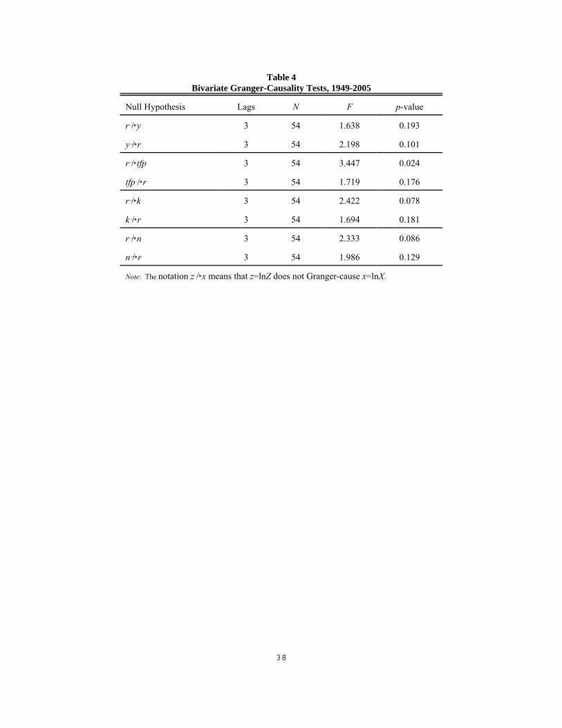
Table 4Bivariate Granger-Causality Tests, 1949-2005

Null Hypothesis Lags N F p-value

r÷/ y 3 54 1.638 0.193

y÷/ r 3 54 2.198 0.101

r÷/ tfp 3 54 3.447 0.024

tfp÷/ r 3 54 1.719 0.176

r÷/ k 3 54 2.422 0.078

k÷/ r 3 54 1.694 0.181

r÷/ n 3 54 2.333 0.086

n÷/ r 3 54 1.986 0.129

Note: The notation z÷/ x means that z=lnZ does not Granger-cause x=lnX.

38

Table 5 - Part IModel Estimates: Regulation Parameters

x = y x = tfp x = n x = k

γ0R 1.06E-06

(8.092)3.93E-07(11.643)

7.07E-07(10.598)

3.84E-07(4.104)

γ1R 2.47E-07

(2.927)-3.42E-09(-0.142)

- -

γ2R -4.17E-07

(-5.283)-1.27E-07(-6.120)

- -

δ0R -4.81E-12

(-9.846)-1.67E-12(-11.792)

-3.33E-12(-9.059)

-1.84E-12(-3.659)

ω0R -0.795

(-3.945)-0.434

(-11.257)-0.304

(-3.164)-0.241

(-1.508)

ω1R -0.415

(-2.625)- -0.366

(-4.416)-0.203

(-1.572)

βRΣωjR -0.039 -0.014 -0.022 -0.014

ΣγjR

F test: ΣγjR = 0

[p-value]

8.90E-0792.156[0.000]

2.62E-0792.053[0.000]

7.07E-07NA[NA]

3.84E-07NA[NA]

ΣδjR

F test: ΣδjR = 0

[p-value]

-4.81E-12NA[NA]

-1.67E-12NA[NA]

-3.33E-12NA[NA]

-1.84E-13NA[NA]

ΣωjR

F test: ΣωjR = 0

[p-value]

-1.210114.561

[0.000]

-0.434NA[NA]

-0.67073.345[0.000]

-0.44316.806[0.000]

Estimation by DOLS includes p lags and q leads of Δrt and Δτt whose coefficient estimates are not reported. Numbers inparentheses (.) are t-statistics corrected for serial correlation using the non-parametric procedure described in Hamilton (1994,608-612) and may be compared to standard t tables. Numbers in braces . are F-statistics corrected in a similar manner andmay be compared to standard F tables. Numbers in brackets [.] are p-values. Numbers do not always add because ofrounding. NA / Not Applicable (when there is only one non-zero parameter, making the sum trivial and calculationof F tests superfluous). The value of βR is 0.0322, as reported in the text.

39

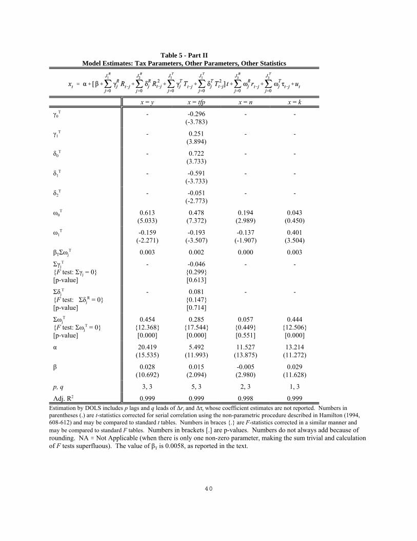
Table 5 - Part IIModel Estimates: Tax Parameters, Other Parameters, Other Statistics

x = y x = tfp x = n x = k

γ0T - -0.296

(-3.783)- -

γ1T - 0.251

(3.894)- -

δ0T - 0.722

(3.733)- -

δ1T - -0.591

(-3.733)- -

δ2T - -0.051

(-2.773)- -

ω0T 0.613

(5.033)0.478

(7.372)0.194

(2.989)0.043

(0.450)

ω1T -0.159

(-2.271)-0.193

(-3.507)-0.137

(-1.907)0.401

(3.504)

βTΣωjT 0.003 0.002 0.000 0.003

ΣγjT

F test: Σγj = 0[p-value]

- -0.0460.299[0.613]

- -

ΣδjT

F test: ΣδjR = 0

[p-value]

- 0.0810.147[0.714]

- -

ΣωjT

F test: ΣωjT = 0

[p-value]

0.45412.368[0.000]

0.28517.544[0.000]

0.0570.449[0.551]

0.44412.506[0.000]

α 20.419(15.535)

5.492(11.993)

11.527(13.875)

13.214(11.272)

β 0.028(10.692)

0.015(2.094)

-0.005(2.980)

0.029(11.628)

p, q 3, 3 5, 3 2, 3 1, 3

Adj. R2 0.999 0.999 0.998 0.999Estimation by DOLS includes p lags and q leads of Δrt and Δτt whose coefficient estimates are not reported. Numbers inparentheses (.) are t-statistics corrected for serial correlation using the non-parametric procedure described in Hamilton (1994,608-612) and may be compared to standard t tables. Numbers in braces . are F-statistics corrected in a similar manner andmay be compared to standard F tables. Numbers in brackets [.] are p-values. Numbers do not always add because ofrounding. NA / Not Applicable (when there is only one non-zero parameter, making the sum trivial and calculationof F tests superfluous). The value of βT is 0.0058, as reported in the text.

40

0

20,000

40,000

60,000

80,000

100,000

120,000

140,000

1950 1960 1970 1980 1990 2000

R HP Filtered

Fig. 1: Regulation over time

R

Year

0.10

0.12

0.14

0.16

0.18

0.20

0.22

1950 1960 1970 1980 1990 2000

MTR HP Filtered Year

T

Fig. 4: Marginal tax rate over time

-0.08

-0.04

0.00

0.04

0.08

0.12

0.16

0.20

1950 1960 1970 1980 1990 2000

DLogR HP Filtered Year

DL

og R

Fig. 2: Growth rate of regulation over time

0.2

0.3

0.4

0.5

0.6

0.7

0.8

1950 1960 1970 1980 1990 2000

Y Ratio: R Effect HP Filtered

Y R

atio

: R

Eff

ect

Year

Fig. 6: Ratio of actual Y to counterfactualY| R=R(1949)

-0.036

-0.032

-0.028

-0.024

-0.020

-0.016

-0.012

-0.008

1950 1960 1970 1980 1990 2000

Y Trend: R Effect HP Filtered

Y T

ren

d:

R E

ffec

t

Year

Fig. 5: Effect of R on Y trend

0

400

800

1,200

1,600

2,000

1950 1960 1970 1980 1990 2000

G HP Filtered Year

G

Fig. 3: Government purchases over time

41

-0.04

-0.02

0.00

0.02

0.04

0.06

0.08

0.10

1950 1960 1970 1980 1990 2000

DLogY HP Filtered Year

DL

ogY

Fig. 7: Growth rate of output over time

-0.04

-0.03

-0.02

-0.01

0.00

0.01

0.02

0.03

1950 1960 1970 1980 1990 2000

TFP Growth: T Effect HP Filtered

TF

P G

row

th:

T E

ffec

t

Year

Fig. 11: Change in ratio of actual TFP tocounterfactual TFP|T=T(1949)

-0.02

-0.01

0.00

0.01

0.02

0.03

0.04

0.05

1950 1960 1970 1980 1990 2000

DLogTFP HP Filtered Year

DL

ogT

FP

Fig. 8: Growth rate of TFP over time

-0.08

-0.06

-0.04

-0.02

0.00

0.02

1950 1960 1970 1980 1990 2000

TFP Growth: R and T Combined Effect HP Filtered

TF

P G

row

th:

R a

nd

T C

omb

ined

Eff

ect

Year

Fig. 12: Change in ratio of actual TFP tocounterfactual TFP|R=R(1949), T=T(1949)

-0.06

-0.05

-0.04

-0.03

-0.02

-0.01

0.00

0.01

0.02

1950 1960 1970 1980 1990 2000

TFP Growth: R Effect HP Filtered

TF

P G

row

th:

R E

ffec

t

Year

Fig. 10: Change in ratio of actual TFP tocounterfactual TFP|R=R(1949)

-0.013

-0.012

-0.011

-0.010

-0.009

-0.008

-0.007

-0.006

1950 1960 1970 1980 1990 2000

TFP Trend: R Effect HP Filtered Year

Fig. 9: Effect of R on TFP trend

TF

P T

ren

d:

R E

ffec

t

42

Appendix: Code of Federal Regulations

A1. History and Background of the Code of Federal RegulationsBefore 1935, no systematic process existed for the promulgation of federal regulations; regulations were

simply typed and filed by individual agencies. The lack of public notification regarding regulatory activity latercame to be known as "hip pocket" law, which led the government to embarrassment in Panama Refining Company v.Ryan (293 U.S. 388, 1935), also known as the "Hot Oil Case."31 The government's case, which was based on aprovision that was later nullified by a subsequent regulation, was dismissed by the Supreme Court, and both partiesin the case were impugned for their ignorance of the law. This outcome led to the Federal Register Act of 1935 (49Stat. 500; 44 USC Chapter 15), which established a consistent framework for codification of government regulationsthroughout the rulemaking process.

The Federal Register (FR), first published on March 14, 1936, is a daily publication in which proposedregulations appear first in draft form and eventually in final form, if passed into law. The FR also containspresidential proclamations, executive orders, announcements of agency hearings and meetings on regulatory issues,grant application instructions and deadlines, official agency decisions and actions, and agency establishments,reorganizations, and dissolutions. Sometimes, there also are long sections containing technical or economic analysesor discussion of issues arising during consideration of a proposed regulation. The final regulations (newly passedinto law) contained in the FR ultimately are codified in the Code of Federal Regulations (CFR). Divided into 50subject categories called titles, the structure of the CFR is similar, but not identical, to that of the United States Code. Currently, each title of the CFR is revised annually and contains all regulations in effect as of the cover date.32

The first edition of the CFR published regulations in force as of June 1, 1938. In the early years, the CFRwas not revised annually. Instead, annual supplements carried in full text all changes and additions to the 1938edition of the CFR as published in the FR. The supplements covered the periods June 2-December 31, 1938 andsubsequent calendar years through 1941, listing regulatory changes promulgated during the period and in effect onDecember 31 of the year in question.33 The first revision of the CFR, scheduled for June 1, 1943 under the FederalRegister Act, was postponed because of the volume of rapidly changing regulations related to World War II and thepreoccupation of all government agencies with the war effort. In its place, a cumulative supplement to the 1938edition of the CFR compiled regulations in force as of June 1, 1943. However, regulations in effect at that datewhose text was identical to that in the 1938 edition of the CFR are included only by reference to the original CFR. Also, emergency controls associated with the war period are recorded by tabulation rather than codification in thecumulative supplement. Thus, the cumulative supplement served as an adjunct to the original edition rather than areplacement of it. Following the cumulative supplement, annual supplements continued to update the 1938 editionof the CFR for regulatory changes published in the FR during the remainder of 1943 and each calendar year through1947. The wartime suspension of the first revision of the CFR was terminated in 1948 and the second edition of theCFR, recording regulations in effect on January 1, 1949, was issued.34

Following the 1949 edition of the CFR, "pocket supplements" were used to record regulatory changes

31Throughout the appendix, the following citation format is used: volume or title number followed by nameof publication followed by page or section number. For example, "49 Stat. 500" designates Volume 49 of the UnitedStates Statutes at Large, page 500. The following abbreviations are also used in the citations: USC for United StatesCode, FR for Federal Register, and CFR for Code of Federal Regulations.

32The U.S. Statutes at Large and U.S. Code are comparable to the Federal Register and Code of FederalRegulations, respectively, except that the former are primarily concerned with the publication and codification oflaws, whereas the later are concerned with transmitting to the public written requirements to be carried out andenforced by government agencies (i.e., regulations). Thus, the CFR is more appropriate than the U.S. Code as ameasure of regulation.

33No supplement was published for 1942.

34Due to the imminence of the second edition of the CFR, no supplement was issued for 1948. Regulatorychanges published in the FR during 1948 were codified for the first time in the 1949 edition of the Code.

A1

published in the FR.35 Pocket supplements differed from the annual supplements to the first edition of the CFR inthat they were cumulative; that is, the pocket supplement for a given year recorded the full text of all changes to the1949 CFR in effect at the end of the given year, irrespective of the year that the change occurred. The first pocketsupplement covered changes during the June 2 to December 31, 1949 period and subsequent pocket supplementsincluded any additional changes in effect at the end of each succeeding calendar year. So, for example, the 1950pocket supplement documents changes to the 1949 edition of the CFR that occurred between June 2, 1949 andDecember 31, 1950. Some of those changes occurred between June 2 and December 31 of 1949 and so already werereported in the 1949 pocket supplement. The 1950 pocket supplement repeats them and adds all changes thatoccurred between January 1 and December 31 of 1950.36

From time to time, as warranted by growth of the pocket supplements, individual titles (or individual partsof a title) of the 1949 CFR were revised. These revisions represented a complete codification of regulations in effectas of December 31 of the year in which they were published. The timing of revisions varied considerably acrosstitles. In all titles, however, revisions became more frequent over time. In 1950, for instance, only Parts 71-90 ofTitle 49 (Transportation and Railroads) were revised. In 1960, all or parts of Titles 1-5, 14, 18-20, 26, 27, 32, 40,41, 49, and 50 were revised, and by 1968, all except Titles 34, 35, and 37 were revised. Beginning in 1969, all titlesof the CFR have been revised annually.37

A2. Measuring Regulatory Activity Using the CFRThe consistent codification of federal regulations in the CFR since its inception in 1938 provides a unique

source of information on regulatory activity over the years. Dawson (2007) constructs series measuring regulatoryactivity based on the number of pages published in the CFR's various editions and supplements. Although thenumber of pages of regulation cannot capture the differential effects of alternative regulations on economic activity,it affords new information on the temporal behavior of the total amount of regulation in place. The remainder of thissection provides a summary of these CFR-based measures of regulation. For a complete description of themethodology used to construct the series and a statistical comparison of the various series, see Dawson (2007).

Before counting pages, we must standardize the pages in the CFR for different words per page across theyears. That turns out to be almost effortless. The CFR uses the same font and page size in all years except the veryfirst, 1938. We converted 1938 pages to “standard” pages simply by multiplying by an adjustment factor based onaverage words per page computed by sampling words per page in each title of the Code. Even this adjustment turnsout to be irrelevant to our empirical work because, for reasons to be explained momentarily, we started our sampleperiod in 1949, thus omitting the non-standard 1938 edition of the Code entirely.38

35The term "pocket supplement" derives from pockets which were made in the books of the 1949 edition ofthe CFR for placement of the forthcoming supplements.

36On several occasions, an "added pocket part" (APP) was published instead of a pocket supplement. TheAPP served as an addition or supplement to the previous year's pocket supplement. APPs were not cumulativeunless they appeared in consecutive years, in which case the old APP was replaced by the current APP as asupplement to the most recent pocket supplement.

37Beginning with the 1973 revision of the CFR, the effective revision date of each title varies within theyear according to the following quarterly schedule: Titles 1-16 as of January 1; Titles 17-27 as of April 1; Titles 28-41 as of July 1; and Titles 42-50 as of October 1.

38There is the possibility that the nature of the language used has changed over time, becoming more or lessverbose as time passes, so that the word-to-regulatory-content ratio changes over time. We have no way to controlfor or even check the existence of such a problem. We know of no evidence that such changes in language occurredover our sample period. Kimble (2002, 2007) has suggested changes in usage that would replace the legalese offederal laws and regulations with more straightforward English, but Kimble himself notes that such changessometimes result in longer rather than shorter documents. Also, we know of no evidence that such suggestedchanges ever have been adopted. Indeed, there is anecdotal evidence that simplification has not occurred. PresidentCarter signed an executive order in 1978 requiring that federal regulations be written as simply and clearly as

A2

Measuring regulatory activity using data on the number of pages in the CFR is straightforward in yearswhen the CFR is revised. These include the years 1938, 1949, all years after 1969, and some years between 1949and 1969.39 Estimating total pages of regulation during the periods between the 1938, 1949, and subsequentrevisions is more problematic. One approach, which explicitly uses all annual and pocket supplement data toestimate total pages of regulation during years in which no revision is published, adds the number of pages in anonrevision-year's supplement to the number of pages in its corresponding complete CFR. The series that resultsfrom this methodology exhibits rapid growth in pages of regulation during most of the 1940s followed by a drasticdecline in 1949. This behavior in part may reflect the increase in regulation associated with World War II and thesubsequent decrease following the war, but it also is likely to reflect in part an element of double counting that is, forpractical purposes, unavoidable with the supplements used to codify regulatory changes between the 1938 and 1949revisions of the CFR. The supplements print the entire text of any section of regulation that changed, even if onlyone word was different. Consequently, a page of text in a supplement may represent completely new text that wasnot present in 1938 or may be almost entirely repetition of previously existing text. The only way to avoid doublecounting repeated text would be to read each reported change to determine how much of it was repetition, anobviously impractical task. Growth in the estimated pages of regulation resumes in the early 1950s and moderatesinto the 1960s. The same double counting problem exists after 1949 as before but is less severe because revisedvolumes of the CFR were published intermittently between 1949 and 1969. The frequency of these intermittentupdates increased as time passed, with almost the entire CFR being revised in 1968. Consequently, the growth in theCFR page count between 1949 and 1969 is much more likely to be a genuine phenomenon than is the pre-1949growth. Double-counting ceases to be an issue after 1968 because the entire CFR is published every year after that. Because the counting problems are much more severe before 1949 than after, we restrict attention in our study to theperiod 1949-2005.40 Also, because we are interested in the effects of regulation on the private economy, we excludefrom our page count all regulations in the first six titles, which pertain to the internal organization and operation ofthe federal government itself.

A3. Comparison with Other Measures of Regulation

A3.1. Description. Our measure covers one country over 54 years; earlier measures cover many countries over muchshorter periods of time.41 Some of the earlier measures are purely cross-sectional, applying to a single year; otherscover more years and so are panel data. The longest time span of the panel sets is 20 years.

Our measure is more comprehensive than any of its predecessors. Federal law requires that all federalregulations be published in the CFR, so our measure includes literally every regulation issued by the federalgovernment. No other measure of regulation comes close to that extent of coverage. For example, the most widelyused of the earlier data sets is the OECD cross-section measure described by Nicoletti et al. (2000) and extended inpart to a 20-year panel by Nicoletti et al. (2001). The cross-section data are restricted to product market andemployment protection regulation; other types, such as environmental or occupational health and safety regulation,

possible. Twenty years later, in 1998, the Clinton administration demanded that regulations be written in plainerprose, suggesting that President Carter's order had not had achieved its goal. We thus proceed on the assumptionthat there have been no significant changes in the verbosity of regulation over time.

39Recall from the discussion above that the timing of revisions to the 1949 edition of the CFR varies acrosstitles between the years 1949 and 1969.

40Dawson (2007) discusses the “double-counting” problem in more detail and offers some alternativemethods for constructing the regulatory series based on interpolation in the non-revision years. The results of theanalysis in this paper are not sensitive to the construction method, thus we restrict attention to the series discussedhere.

41See Nicoletti et al. (2000), Nicoletti et al. (2001), Djankov et al. (2002), Kaufman, Kraay, and Mastruzzi(2003), Nicoletti and Scarpetta (2003), Loayza et al. (2004), and Djankov et al. (2005) for detailed descriptions ofthese alternative measures.

A3

are ignored. The panel extension is restricted further to a small subset of seven non-manufacturing industries: gas,electricity, post, telecommunications, passenger air transport, railways and road freight. Types of regulationsconsidered also are limited, with data availability varying by industry: barriers to entry (available for all industries),public ownership (all industries except road freight), vertical integration (gas, electricity and railways), marketstructure (gas, telecommunications and railways), and price controls (only road freight).

All measures of regulation including ours are aggregate indices. Our index is more highly aggregated thanany of the others simply because it covers the full array of regulations, but all are aggregates. None simply reports aquantitative measure of the magnitude or effect of a single regulation. The OECD measure, for example, collectsanswers to about 1300 questions and combines them into an index through a multistep aggregation procedure. Themethods of aggregation differ substantially across indices. Our method is to weight each regulation by its number ofpages in the CFR, which captures at least partially the complexity of the regulation, as we discuss below. Manyother indices are constructed as simple averages of basic data, with no attempt to weight by the importance orcomplexity of the regulations included. The OECD uses a multistep procedure, in which the OECD staff creates acollection of categorical sub-aggregates mostly as simple averages of basic data and then uses factor analysis toaggregate those into its final indices.

All measures except ours are based at least in part on survey data, typically obtained from questionnairessent to government officials (OECD), market participants (Kaufman et al.), and/or lawyers (Djankov, 2002). Ourmeasure is based solely on the page count of the CFR.

A3.2. Evaluation. Our measure is a pure time series covering a long time span. The earlier measures of regulationhave short to non-existent time spans, the longest being 20 years and the shortest 1 year. Such data cannot be usedto study regulation's effects on macroeconomic dynamic adjustment paths, which requires following the evolution ofvariables through time. There is more hope of studying regulation's effects on average growth rates by using thecross-sectional dimension of the data to overcome the inadequate time dimension, which is precisely what several ofthe previous studies do. However, growth is an intertemporal phenomenon, so it would be useful to have time seriesestimates of regulation's effects on it, especially in light of Ventura's (1997) demonstration that the interpretation ofcross-country growth regressions is confounded by the effects of foreign trade. Our measure, with its comparativelylong time dimension, allows us to study both the long-run growth and short-run dynamic adjustment effects ofregulation. The earlier studies, with their strong cross-section element but weak intertemporal element, are bettersuited for cross-sectional issues.

Our measure also is more comprehensive than the earlier measures, none of which encompasses the total setof regulations in any country. Incomplete coverage leads to two problems: (1) omitted variables bias, and, in anytime series study, (2) divergence between the time series behavior of subsets of regulation on the one hand and oftotal regulation on the other.

Table 1 shows that the page counts of the various titles of the CFR are highly correlated with one another,whether measured in levels or growth rates. The mean correlation among levels is 0.60, with an even higher medianof 0.77. The maximum correlation in levels is 0.99, and the minimum correlation is -0.76. The correlations ingrowth rates are much lower, of course, with a mean of only 0.16 (median of 0.15), but there still are quite a fewcorrelations of substantial magnitude, with the maximum and minimum being 0.74 and -0.63, respectively.42 Suchhigh correlations show that including just one type of regulation in a statistical analysis is likely to be misleadingbecause of multicollinearity and consequent omitted variables problems. The problem is even more severe whenaddressing issues of macroeconomic dynamics. The correlations in Table 1 are all contemporaneous; for analyzingtime series behavior, we also want to know the dynamic relations among various types of regulations. Granger-causality tests show the intertemporal dependence of one series on another after accounting for the first series'sdependence on its own lagged values. Table 2 summarizes Granger-causality test results for two titles of the CFRrelated to the kinds of regulations studied in previous analyses–regulation of entry and regulation of labor markets. Title 16 of the CFR pertains to Commercial Practices, and Title 29 pertains to Labor. Table 2 shows that the pagecounts of those titles both Granger-cause and are Granger-caused by the page counts of other titles, some apparentlyquite unrelated in content to the subjects of titles 16 and 29. Similar results hold for most of the other titles of theCFR. These Granger-causality relations among CFR titles show that there are temporal orderings in the statistical

42Similarly, Loyaza et al. (2005) found very high correlations among their 7 indices of regulation.

A4

relations among the types of regulation and provide strong evidence that a time series analysis restricted to a subsetof regulations is likely to suffer from serious omitted variables bias.

The foregoing remarks have greatest force when applied to attempts to study the economic effects of aparticular type of regulation. If one is interested in the impact of total regulation, the high correlations among thedifferent types might actually be considered good news because they suggest that a subset of regulations may capturethe behavior of the whole. Indeed, Nicoletti et al. (2001), who have perhaps the most restricted measure of all,interpret their indicators as “a proxy for the overall regulatory policies followed by OECD countries over the sampleperiod (p. 43).”

Unfortunately, examination of the data shows this hope to be ill-founded. Nicoletti et al.'s (2001) measurespans 1978-98 and shows a 66% decline over that period. Subsets of CFR titles corresponding to Nicoletti et al.'smeasure behave similarly. For example, titles 23 (Highways), 46 (Shipping), and 49 (Transportation) of the CFRencompass regulation of air transport, railways, and road freight, one Nicoletti et al.'s regulation groups. The pagecount of titles 23, 46, and 49 drops from a total of 8400 in 1978 to 8261 in 1998, which is qualitatively the samebehavior as Nicoletti et al.'s measure. Nevertheless, the page count of the total CFR displays the opposite behavior,rising 47% over 1978-98. The inescapable implication is that subsets of regulation are not reliable proxies for totalregulation.

Our measure of regulation is the only measure constructed by a completely objective method. Our measureconsists of the page counts in the CFR, a number requiring no judgement to obtain. Subjectivity enters all othermeasures in two ways. First, as remarked above, all other measures are based at least in part on survey data. AsNicoletti et al. (2000) note, the people completing the surveys have some latitude in interpreting the survey questionsand may respond idiosyncratically. Second, the survey must be designed and the responses must be combined,processes that involve the judgement of the investigator. For example, the OECD index begins with responses toabout 1300 survey questions. The responses usually are Yes or No. Groups of these responses are combined byaveraging to create categorical variables with values from 0 to 6. The procedure used for measuring the scope ofpublic enterprise illustrates the issues. Respondents are asked if there are “national, state or provincial governmentcontrols in at least one of” 24 industries chosen by the OECD. Some of the industries chosen are 2-digit ISIC (e.g.,wholesale trade, financial institutions), some are 3-digit (e.g., tobacco manufactures), and some are 4-digit (e.g.,electricity, motion picture distribution and projection). Despite the differences in size and importance, all industrieshave been assigned the same weight of 1 in the construction of the categorical variables. See Table A2.1.1 inNicoletti et al. (2000), p.60, for details.43 Other measures of regulation are generally more subjective than theOECD's. An oddity that results from subjectively deciding what is and is not regulation is that two of the publishedmeasures of regulation contain elements that have nothing to do with regulation. The OECD measure includes dataon publicly-owned enterprises, a form of government intervention but not regulation. Loayza et al.'s (2005) measureincludes data on spending and taxation and on the fraction of the workforce that is unionized, neither of whichpertains to regulation. These measures thus confound regulation with other government and even non-governmentactivities.

Some indices of regulation attempt to measure the burden imposed by the component regulations byincluding quantitative and/or qualitative data pertaining to the regulations included. Examples include the number ofprocedures a new firm must go through to start operation (Djankov et al., 2002) and regulatory complexity (OECD;Nicoletti et al., 2000). Our measure contains no such direct measures but nonetheless controls for regulatory burdento some extent. It seems reasonable to suppose that, on average at least, the more complex a regulation, the morepages it will require. Indeed, the OECD measures complexity by the presence or absence of a long list of regulatoryrequirements. The larger the number of requirements, the more the pages of regulations necessary to describe them,which is precisely what our measure captures. Indeed, our approach may give a more complete picture of regulatoryburden than the OECD's measure because page counts indicate not only the presence or absence of particularprovisions but also their complexity.

43Nicoletti and Pryor (2001) argue that the OECD measure is objective, but it clearly is not. Indeed, indescribing its construction, Nicoletti et al. (2000) say that 90% of the data underlying the OECD measure is “surveydata” (p.11) and that both questionnaire responses and the procedure for scoring them involved “subjectivejudgement” (p.16).

A5

A3.3. Summary. Our page count measure of the extent of regulation compares well with other measures. Althoughlimited to a single country, it has a much longer time span than any other measure. It is unique in being totallycomprehensive.44 It also is unique in being 100% objective both in the data underlying it and in the method ofconstructing the index. It offers indicators at two levels of aggregation–one final index for total regulation and manysub-indices for the different classes (“titles”) of regulation. It is easily replicated and easily updated. Finally, CFRpage counts are a more precise measure of regulation than page counts of other federal publications, such as theFederal Register or the U. S. Code, suggested by others.45 The Federal Register contains proposed regulations andother irrelevant material; the U. S. Code contains all federal laws, not just regulations.

44At least for federal regulations. Our measure does not include state and local regulations.

45Friedman and Friedman (1979) use the number of pages in the Federal Register to measure the growth ofregulation. Becker and Mulligan (1999) use pages in the U.S. Code as a measure of growth in the size ofgovernment. Mulligan and Shleifer (2003) use kilobytes of unannotated state law, where 1kb approximately equalsone printed page, to study the causes of regulation.

A6