2~ Forwardied by:us AROY STAN DARDIZATIO',, GREY V

UNIEDKINGDOM

-~~ 65031 us FIgo NO, Nw Yorks Wt.rO9iI

FEBRUARYROYAL AIRCRAFT ESTABLISHMENT

1965 cl ýp TECHNICAL REPORT No. 65031

CALCULATION OF OPTICAL

TRANSFER FUNCTIONS FROM

LENS DESIGN DATA

by

TE11OAL LIERARYA. C. Marchant BD 1

Margaret Lello TAh

MHE RECIPENT IS \W A KNEU IH rCONhTAINE3D IN TVH!S( C;C PIT *

TO PRIVAT',ELY-0O;v- IucH.;

U.D.C. No. 535.316/317

ROYAL AIRCRAFT ESTABL IS.HMENT

Technical Report No.65031

February 1965

CALCULATION OF OPTICAL TRANSFER FUNCTIONS

FROM LENS DESIGN DATA

by

A. C. Marchant

Margaret Lello

SUMMARY

This Report describes the basic theory and the method of operation of a

computer programme developed at Imperial College, London,for calculating the

optical transfer function of a lens system. The programme determines the wave-

front aberration, and the shape of the exit pupil (vignetted or otherwise) and

uses this information to derive the transfer function in any image plane and at

any field angle. Typical results, for a modern aerial reconnaissance lens, are

given and compared with measurement.

ALCUDEBaT HqflQVmG. GFUI, HID,

Departmental Reference: IEE 80

T•IlO&L TJ IBhAEBLDO B13

A3BRD~ b1'pOVLNG GROMI •0.STBA:P-'r

2

CONTENTS

I INTRODUCTION 3

2 THEORY OF IMAGE FORPJATION 4

2.1 Fundamentals 4

2.2 "Sine wave" objects 5

2.3 Incoherent illumination 5

2.4 Effects of lens aberration 6

2.5 General application of the theory 6

3 BASIC FORIMiULAE 7

4 METB1OD OF C01h1UTATION 9

4.1 Calculation of wavefront aberration 9

4.2 Determination of effective pupil area 10

4.3 Calculation of transfer function 11

4.4 Relation of spatial frequency to the variable s 12

5 TRANSFER FUNCTIONS IN "WHITE LIGHT" 13

6 OPERATION OF COMPUTMR PROGRA11MES (M. Lello) 14

6.1 Introduction 14

6.2 Programme A: Calculation of wavefront aberration and 14pupil shape

6.3 Programme B: Selection of "best focus" 16

6.4 Programme F: Determination of transfer function curves 18

7 RESULTS 19

8 ACKNOWLEDGEMENTS 20

Appendix Derivation of the basic diffraction formulae 21

References 23

Illustrations Figures 1-16

Detachable abstract cards

3

1 INTRODUCTION

The merits of the optical transfer function as a means of assessing lens

performance are now well established '

By analogy with other communication processes, an optical system is

regarded as a low-pass, linear, filter whose characteristics can be specified by

means of transfer, or frequency response, curves showing the variation of anmli-

tude and phase of a transmitted signal with its spatial frequency. In the

present context, the "signal" is represented by a two-dimensional grating-like

object consisting of infinitely long parallel lines, the light intensity varying

sinusoidally between one line and the next. The "amplitude" is half the differ-

ence of intensity between brightest and darkest parts of the pattern (Fig. 1).

"Phase" denotes a lateral displacement of the lines in a direction perpendicular

to their length, and is expressed as the ratio of this displacement to the line

separati on.

"Frequency" is the reciprocal of this separation, usually quoted as the

number of lines per millimeter.

To accord with visual impressions, amplitude is usually related to

"contrast" which is itself defined as the ratio of amplitude to mean intensity.If I and I m represent maximum and minimum intensities in the pattern, then

max mmn

1Ia -mi)/2 I1- 1

Contrast = max m max mini +I.

max min max min

A plot of contrast and phase against spatial frequency (see Fig.1 6 ) gives

complete information about the image-forming properties of a lens system, and

allows a. precise assessment to be made of its performance when used with any

given image receiver or sensor. Recent advances in diffraction theory make it

possible to calculate transfer curves from lens design data, so that it is now

practicable to investigate which of a number of available designs will meet a

given functional specification without having to manufacture a prototype lens

and test its performance under the actual conditions of use.

This Report describes the main features of a computer programme, (recently

developed under Ministry of Aviation sponsorship by the Imperial College of

Science and Technology) the method of operation, and finally gives some examples

of the results obtained.

4 03

2 THEORY OF IMAGE FOIMUiATION

2.1 Fundamentals

The theory underlying this method of calculating optical transfer functions

3is based essentially on Abbe's theory of image formation

As these ideas are not generally familiar, it is worthwhile to outline

them briefly before describing their extension in the present work.

Abbe was primarily concerned with imagery in the microscope. Fig.2 illus-

trates the conditions obtaining with so-called "K*6hler" illumination of the

object G, in which light from each point of the source s is rendered parallel by

the condenser c before passing through the object. For simplicity we will assume

initially that the source is very small, and that the object is a simple grating

of opaque sharp-edged lines and clear spaces. The parallel beam passing through

the grating then gives rise to a Fraunhofer diffraction pattern behind the

microscope objective M. This pattern consists of a number of secondary images

of the source; ray paths to two of these (-1 and i) are shown in the figure

and others are indicated by 2, 3, 4 etc.

Now according to Abbe the image of the grating, formed in the plane G',

can be thought of as an interference pattern formed by the light from all these

secondary (coherent) sources.

Thus the pair I and -1 acting alone would give a pattern of interference

fringes, in which the light intensity varies co-sinusoidally with distance from

the axis GG', the separation of the fringes being dependent on the separation of

the two sources and on the distance OG'.

Similarly, the pair 2 and -2 acting alone, would give a fringe separation

of half that in the previous case, 3 and -3 would give still more closely spaced

fringes, and so on.

The final image is the combination of all these separate interference

patterns with the uniform illumination provided by the central source 0, and is

a perfect reproduction of the object provided the objective is free from aberra-

tion and accepts all the diffracted light from the grating. This can in actualpractice never be the case (because the objective would require to be of infinite

aperture) so that the image is always degraded. If the aperture of the objective

is reduced so far that only the light contributing to "sources" -1, 0 and I is

accepted, then the final "image" is a nearly sinusoidal fringe pattern, instead

of the sharp-edged pattern required, although the fringe spacing is the same as

the bar spacing would be in the ideal image.

5

2.2 "Sine wave" objec.ts

At this point it is necessary to define more precisely what is meant by

the "sinusoidal" grating object referred to in Section 1. The simple fringe

pattern which represents the image of such an object can be produced by only two

diffraction maxima, equally spaced each side of the optical axis.

The amplitude A(x) of the wavefront, immediately after transmission

through the grating, varies with distance x (measured perpendicular to the bars)

across it in the following way:-

A(x) = A cos (2.1)

where A is a constant, and L the distance between neighbouring bars, or the

spatial "wavelength".

Equation (2.1) defines the optical "signal" with which we shall be

concerned in this Report,

Because of the negative values of amplitude associated with this expression,

and the absence of a central order in the diffraction pattern, such a grating

would have the physical form illustrated in Fig.3. The transmission varies

continuously from zero at the centre of a bar to a maximum at the centre of the

adjacent space, and each alternate bar is covered by a transparent phase-

changing strip which produces a retardation of A in the phase of the light

passing through it. The three right-hand drawings show respectively the shape

and the variation of amplitude and intensity of the wavefront leaving the

grating.

2.3 Incoherent illumination

The discussion so far has been restricted to coherent illumination of the

object, that is to say it is assumed that a fixed phase relationship exists

between wave elements emerging from different parts of the grating. This implies

that a single radiating source is involved. The more general case of incoherent

illumination is represented by an infinite extension of the light source s in

all directions, in a plane indicated by the dotted line in Fig.2. An infinite

number of independently radiating sources are now present, each one providing

a parallel beam through the grating. One such beam is illustrated by the

chained lines in Fig. 2. -With the sinusoidal object defined in the previous

section, each beam provides a pair of diffraction maxima, and the final image

is the sum of all the separate fringe patterns, each of which arises from one

pair of maxima.

6

Fig.4(a) shows a view of the aperture of the microscope objective as seen

from G'. Suppose the spatial frequency of the grating is such that the maxima

it produces are spaced by a distance s. Two such maxima are indicated by the

points AA in Fig.4(a). An infinite number of other pairs with separation s will

be present in the aperture, but will be confined to the two shaded areas, because

the companion to any maximum which lies outside these areas will not fall within

the lens aperture and will not therefore contribute to the interference patterns

in the image plane.

The points BB in the figure represent such a "forbidden" pair.

2.4 Effects of lens aberration

The point has now been reached at which it is necessary to consider how the

final distribution of intensity in the image plane depends on the diffraction

pattern behind the objective, or in what is strictly the exit pupil of the system

shown in Fig.2. If all the secondary sources radiate with the same phase in a

spherical surface centred at the image point G1, there will be a maximum of

intensity at this point since by Huygen's principle the wave elements emitted

from each source pair in the surface have equal distances to travel and will

interfere constructively. The total effect at G' is found by summing the

intensities of all the separate interference patterns, and the image of a "bright

bar" of the original grating appears at this point.

Exactly the same conditions apply at other points in the neighbourhood of

G' at which other bright lines of the grating are imaged. (It should be

emphasised that in this theory one is concerned essentially with very small scale

effects, and with areas of the image plane which are vezo small compared to their

distance from the exit pupil of the optical system.)

If the lens system introduces aberration, the phases of the diffraction

maxima are no longer equal in the spherical reference surface, and complete con-

structive interference does not occur at G' and similar points. The general

effect is that the "contrast" (see Section i) of the image is reduced and there

may also be a slight lateral movement, or "phase shift" of the lines,

As will be shown later, it is possible, given the wavefront aberration of

the lens system, and consequently the relative phases of the diffraction maxima

in the exit pupil, to calculate the contrast and phase of the image accurately.

2.5 General application of the theory

Although Abbe's theory was originally applied to the microscope, the same

ideas can readily be extended to any other type of optical system.

.31 7

For example, with the photographic lens the object would be nominally at

infinity. The light leaving it would normally be incoherent and the object could

be simulated by a transparent grating with a large "effective source" (previously

represented by the plane s and condenser c in Fig.2) behind it.

The diffraction maxima are formed in the entrance pupil of the lens system,

now infinitely distant from the grating. They are then imaged through to the

exit pupil with phase variations imposed, due to the aberrations of the lens

system, and the final image is formed by interference in the focal plane.

3 BASIC FOP1,ULAE

A simplified derivation of the fundamental formulae will now be given:

for a more rigorous treatment the work of Hopkins4 should be consulted. The aim

here is primarily to illustrate the physical principles involved.

Consider the interference of waves from a. pair of maxima AA, separation s

(Fig.5) formed by a simple sine wave grating.

Let the phases of these maxima, in the spherical reference surface centred

at G' and passing through the centre E of the exit pupil, be represented by

Sand (x,y a x-s,y

Then the complex amplitude at a point P of the image plane in the neighbour-

hood of G' is given by:-

8A(u,v) =e ix'y i ux+vy) + e ix.-s'y ei[u(x-s)+vy]

(see Appendix)

where u and v are the coordinates of P.

To find the resulting intensity at P, the above expression is multiplied

by its complex conjugate, giving

81(u,v) = 12 + 2 cos(us - [0,y -¢x-spy M

The intensity therefore varies sinusoidally with distance u across the image

plane, reaching a maximum value of 4 and a minimum value of zero. The contrast,

by the definition of Section 1, is therefore unity and is independent of the

separation s of the sources. Since this separation depends on the line-spacing

in the object and also controls the line-spacing in the image, it follows that

the contrast in the image is independent of spatial frequency, when only a single

source-pair is involved (coherent light). The position of the lines in the

8 I

image plane, however, depends on the phase term [¢x.y - Ox-sIyI and this will

vary according to the position of the source-pair in the exit-pupil,

For a single spatial frequency and incoherent illumination, therefore,an

infinite number of sinusoidal patterns, all of the same contrast, appear in the

image plane, the peaks of one pattern being slightly displaced from those of

another. The resultant effect is found by summing the intensities of all the

patterns at each point in the image plane. Hence

1(u,v) = 2 [I + cos(us - [x,y x-s,y dx dy

S

The integral is taken over the area S of the exit pupil within which the effec-

tive source-pairs lie (See Fig.4), each source effectively covering aa elemen-

tary area dx dy of the exit pupil. To this expression must be added the con-

tribution of single sources covering the "forbidden" area of the exit pupil

(unshaded area in Fig.4) which -an be written as

I(u,v)As = 2/j] dx dy

A-S

where A denotes the whole area of the exit pupil.

Expanding the cosine in the previous expression then gives

I(u,v) = 2 dx dy + 2 cos(us) if coS[xy -xsy dx dy

A S

+ 2 sin(us) ffsin[¢x~ y - xy dx dy

when terms which are invariant with x and y are taken outside the integral, and

the "single source" term has been added.

The last equation again represents a sinusoidal distribution of the form

I(u,v) = C + D cos(us - •) (3.1)

in which C denotes the term 2. dx dy and

A

9

D 2 27]cos(ox, X. )dx dy] +1 l 'sin(ox O dx dY

S S

(3.2)

and

1 ° os(¢~ xsy x

The contrast in the image is now

T(s) = D/c (3.4-)

and the pattern has a resultant phase shift C. Both these factors can be

calculated if the phase difference [0xy - Ox-syI is known, and hence the

required transfer function curve of contrast and phase shift against the spatial

frequency variable s (see Section 4.4) can be plotted.

This simple derivation of the optical transfer function formulae applies

strictly to axial imagery. However, the more detailed treatment of Hopkins

shows that the same formulae may be applied when the point P of Fig.5 lies well

away from the optical axis EG'. In this case, distances in the image plane are

referred to the intersection point of the principal ray with the image plane as

oi igin.

4 MErHOD OF COMPUTATION

4.1 Calculation of wavefront aberration

The determination of the required phase differences in the exit pupil

requires a knowledge of the wavefront aberration5 of the lens system. Fig.6

shows a distorted wavefront (solid line) passing through the exit pupil of a

system, and the reference sphere (dotted line) which has the same radius of

curvature at the pole E. G',the centre of the reference sphereis then the par-

axial focus of the system.

The line QP represents a ray, necessarily normal to the wavefront, which

intersects the reference sphere at M. The distance YQ is the wavefront aberra-

tion W and the phase of the disturbance at M leads on that at Q by an amountx~y

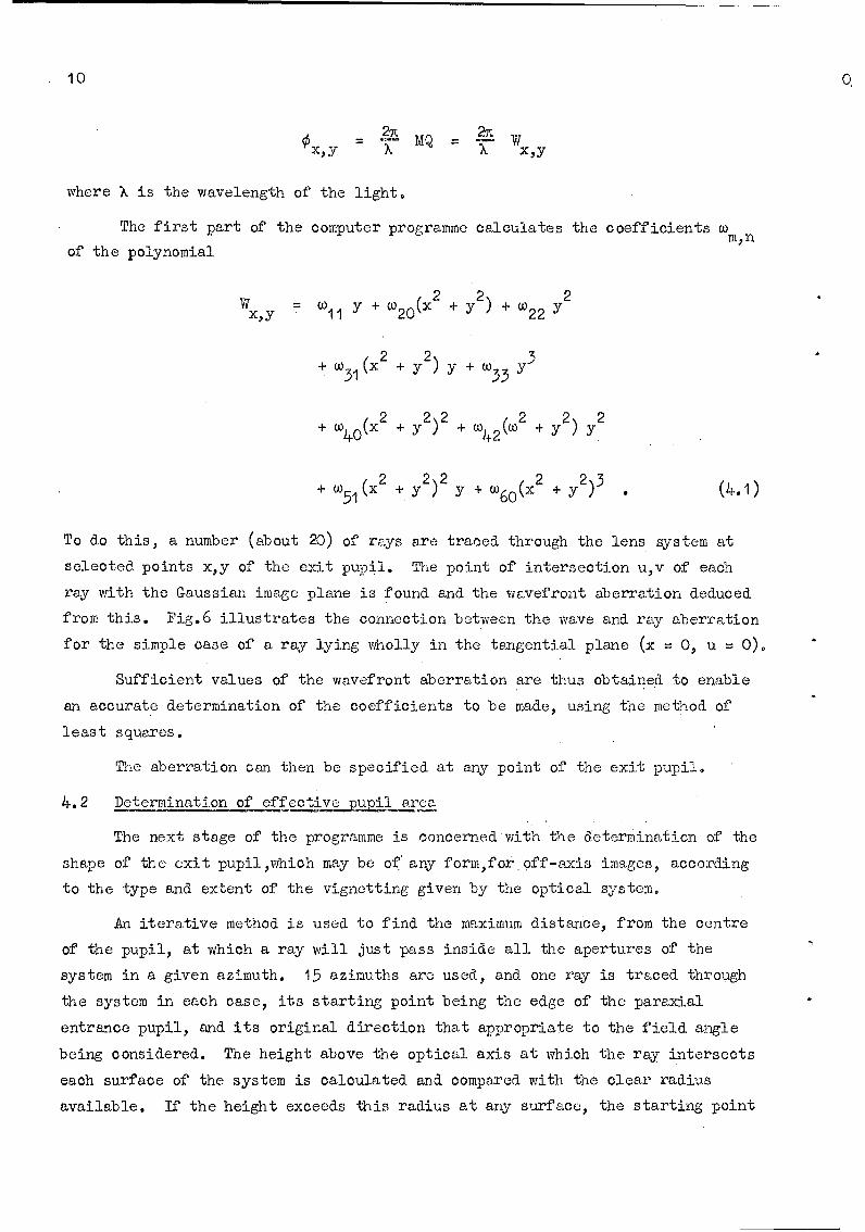
* 10 Q.

2x 2• yS' T MQ =-~- Wx

where W is the wavelength of the light.

The first part of the computer programme calculates the coefficients wm,n

of the polynomial

W = 1 y + W20 (2 +. y ) + o022 y

2 2+W31 33y2 . y +

"+ W40(x 2 + y 2 ) 2 + + Y) 2

"+ W5 1 (x 2 + y2 )2 y + (60(x2 + y 2 ) 3 . (4.1)

To do this, a number (about 20) of rays are traced through the lens system at

selected points x,y of the exit pupil. The point of intersection u,v of each

ray with the Gaussian image plane is found and the wavefront aberration deduced

from this. Fig.6 illustrates the connection between the wave and ray aberration

for the simple case of a ray lying wholly in the tangential plane (x = O, u = 0).

Sufficient values of the wavefront aberration are thus obtained to enable

an accurate determination of the coefficients to be made, using the method of

least squares.

The aberration can then be specified at any point of the exit pupil.

4.2 Determination of effective .uil area

The next stage of the programme is concerned with the determination of the

shape of the exit pupil,which may be of any form,for off-axis images, according

to the type and extent of the vignetting given by the optical system.

An iterative method is used to find the maximum distance, from the centre

of the pupil, at which a ray will just pass inside all the apertures of the

system in a given azimuth. 15 azimuths are used, and one ray is traced through

the system in each case, its starting point being the edge of the paraxialentrance pupil, and its original direction that appropriate to the field angle

being considered. The height above the optical axis at which the ray intersects

each surface of the system is calculated and compared with the clear radius

available. If the height exceeds this radius at any surface, the starting point

31 11

is brought nearer the axis by a small increment s and the ray retraced.. This

process is repeated until the ray passes through the system, and its coordinates

x and y in the exit pupil are recorded as defining a point on the periphery of

the exit pupil (Fig.7). The particular surface which limits the ray height is

also noted.

The increment s is chosen to suit the size of the system being investigated:

clearly the boundary of a large pupil need not be defined as exactly, in absolute

measure, as that of a small pupil, and computing time is thereby reduced. Thefinal result of this part of the prograrmme is a set of 15 coordinates defining

points round one half of the pupil periphery, the pupil being symmetrical about

the tangential plane shown by the y-axis in Fig.7. The "centre" of the off-axis

pupil is taken as the point 0 midway between the rays I and 15.

'When the pupil shape has been determined, the effective area occupied by

all the source-pairs at the separation s can be found. This is in fact the area

common to, two overlapping pupil shapes separated by the distance s. It will be

clear in Fig.4(b) that this included area has the same shape as the two

(identical) areas of Fig.4(a), and the same result applies to non-circular

pupils.

4.3 Calculation of transfer function

When the wavefront aberration and exit pupil coordinates of an optical

system have been established by ray-tracing, the components T(s) and 4 of the

transfer function can be derived as outlined in Section 3 above.

The integrals involved can be evaluated analytically only in the very

simplest cases; generally a numerical teclmnique, such as that described below,

has to be used.

One simple and very important case which can be solved analytically is

that of the in-focus, aberration-free system. Here the phases 0x,y

(equations (3.2) and (3.3)) are all zero and the transfer function reduces to:-

T(s) = D/C dxdy/Jidxdy ; =0

S AThus the contrast in the image depends solely on the ratio of the effective to

full area of the exit pupil.

This ratio, for a circular pupil, is given by

T(s) = 1 [2 cos- 1 (s/2) - sinJ2 cos 1 (s/2)j] . (4.2)

12

Values of T(s) versus s for this case are plotted in Fig.8 (solid line).

For the general case of a vignetted pupil, and a full aberration function

(see equation (4.1)) the integration is carried out numerically by covering the

effective area of the exit pupil with a square mesh (Fig.7); and determining a

weighted mean value for the aberration within each square. The number of squares

contained within the pupil and within the region of overlap (Fig.4(b)) is calcu-

lated, and also the phase difference (0 - x- ), of equations. (3.2) and

(3.3), at a series of points separated by a distance equal to the length of side

of the squares, and lying in the overlap region.Equations (3.2) and (3.3) can then be applied to find the transfer function,

the integrals now becoming sums, the number of terms in which are equal to the

number of squares within the overlap-region. The constant term C (equation (3.1))

is of course represented by the number of squares in the complete pupil.

The accuracy of the final result' is clearly dependent on the size of the

mesh. Fig.8 illustrates the kind of errors which arise from the finite size of

square, when the transfer function of an aberration-free lens is calculated by

this numerical process. The original computer programme has since been modified

so that the number of squares contained in the effective area is never less than

1000, the square size decreasing as the separation s increases. Under these

circumstances the error in T(s) should never exceed 0.01.

This description of the theory underlying the computer programme has

assumed a horizontal separation of secondary sources, that is to say an orienta-

tion of the object grating so that its lines lie radially in the lens field

(parallel to the y-axis in Fig.7)o

However, the same techniques may be used to calculate the response for any

other orientation of the grating, and. in practice the programme caters for

orientations of 00 (radial lines), 900 (tangential lines), and any angle between

these.

4.4. Relation of spatial frequenc to the variable s

It has already been shown -that the spatial frequency of the lines in the

image plane depends on the separation s of the' secondary sources in the exit

pupil.

The frequency is usually expressed as the number of lines per millimeter

in the image plane.

Equation (3.1) above shows that the intensity repeats its value at distances

u = 2%/s apart in this plane, and this is therefore the "spatial wavelength" of

13

the sinusoidal pattern. Coordinates in the exit pupil are actually expressed

as fractions of its maximum radius (specifically the radius of the paraxial

pupil - see Appendix) and s is of course in the same units. If S is the actual

separation of the sources, the fractional value is:

S - X 43max

where X represents the maximum pupil radius (see Fig.5). Distances in the.maximage plane are also expressed in "reduced" coordinates viz:-

u X (Appendix - Equation (A,1))

R X max

so that the intensity repeats at intervals

2,n 2gXs g max

g is the actual length of one period in the image plane, and the spatial fre-

quency v is given by

Xmax*lV 1/g - X

In the ccmmonest case, that of a photographic lens with the object at

infinity:

The maximum source separation which will provide a fringe pattern in the

image plane, is equal to the diameter of the exit pupil. Thus in the expression

(4,3) above, Smax 2 X max and s m =22.

This represents the ultimate resolution limit of the optical system, since

with wider separations only one source lies within the aperture at a time, and

the illumination bf the focal plane is uniform. For a relative aperture of f/8,

and a wavelength of 5 x 10-4 mm, this limit is reached at v 250 &/mm.

5 TRATSFNR FUNCTIONS IN "WHITE LIGHT"

The foregoing discussion refers, of course, to monophromatic illumination

of the object. In most practical cases a continuous spectrum is involved, and

the problem remains of synthesising the transfer function applying in these

14 O5

conditions from the results calculated at a number of discrete wavelengths. In

principle, this can be done by adding corresponding ordinates of these "mono-

chromatic" response curves, after multiplying each by a factor proportional to

the intensity or sensitivity of the light source and receiver (photographic

film, television tube etc) taking account of the relative spatial phase at each

wavelength.

In practice, two main problems arise: firstly, how many separate wave-

lengths need be specified to yield an accurate "white light" result, and secondly

what is the most efficient method of selecting the best image plane in which to

find the "combined" transfer function.

These points are under investigation at the time of writing, and the

results reported in the second half of this Report refer only to monochromatic

light.

6 OPERATION OF COMPUT]Mi PROGRYIMES

6.1 Introduction

The three sub-programmes to be described (designated A, B and F),cover

three separate phases of the calculation of optical transfer functions.

Programme A takes the lens design data and calculates the wavefront aberra-

tion and the shape of the exit pupil, for given object/image conjugates and field

angles.

Selection of the best focal plane in which to calculate the transfer func-

tion is done by means of programme B, and programme F determines the contrast

and phase curves in the chosen focal plane, at the given field angle.

The programmes are written in Mercury Autocode; programme F has recently

been modified slightly to enable it to be used on the "Atlas" computer. "Atlas"

is about 60 times faster than "Mercury" and has a greater storage capacity; this

allows the use of a smaller mesh size, and hence an increase in accuracy (see

Section 4.3).

The operation of these programmes will be illustrated by means of an

example, viz. a 24 inch f/5.6 reconnaissance lens of new design. It will be

shown how the designer's data are used in programme A, and the way in which the

results from this are used in programmes B and F.

6.2 Programme A: Calculation of wavefront aberration and ,_pil shiape

This programme calculates the wavefront aberration (Section 4.1) for three

wavelengths both for the axial case and for one selected field angle. The pupil

15

shape for this angle is given in the form of 15 coordinates (x,y) round half the

pupil, which is symmetrical about the y-axis (Fig.7). As mentioned previously

the x,y actually used are "reduced" coordinates obtained by dividing actual

distances from the axes by the radius of the exit pupil*.

Fig.9 shows the data as received from the lens designer, and Fig.lO the

form of the data tape produced from this. In counting the number of surfaces,

the stop is included, and where two surfaces are cemented together only one is

counted.

Starting values for a paraxial marginal ray have to be chosen, u being the

angle the ray makes with the optical axis, and h the height above the axis of

the edge of the paraxial entrance pupil. The sign convention used for the angle

is that an anti-clockwise rotation from ray to axis denotes a positive angle.

With object at infinity, u = 0 and h = (focal length)/2(f/no.). With a finite

object distance u and h must be deduced from simple paraxial considerations.

As explained in Section 4. 02, the accuracy s to which the shape of the exit

pupil needs to be defined depends on the actual size of the system. The condi-

tion that a ray shall pass through a given surface is

p < (Free aperture) + e

where p is the distance between the optical axis and the point at which the ray

intersects the surface.

Refractive indices for commonly used wavelengths can be obtained directly

from the glass catalogue; other wavelengths can be interpolated using a suitable

dispersion formula7.

The field angile 6 can have any value other than O° and the Lagrange

invariant (H) is given by:-

SH h tan 0

when the field angle is measured from the centre of the paraxial entrance pupil

for a finite object distance.

The programme tape takes about 6 minutes tobe read into Mercury. Each

set of data takes about 2 minutes to calculate.

*Strictly, the radius of the pupil, in the sagittal plane, calculated by paraxial

formulae.

16

At the end of a set of data, the machine will return to the beginning of

the programme, so that for results for another field angle, the complete set of

design data must be read in again.

Fig.11 shows the form in which the results are presented.

The "reduced height of exit pupil" gives the ratio of the actual on-axis

pupil radius, to that of the paraxial pupil. Under "pupil shape", Q defines

which of the 15 "peripheral rays" is being considered (see Fig.7), S denotes the

surfaces which limit the off-axis beam in this azimuth (more than one surface

may limit a ray within the tolerance s) and X' and Y' give the coordinates of

the exit pupil periphery.

The "exit pupil scale ratio" gives the relationship between the numerical

apertures of the off-axis and on-axis exit pupils. This ratio is used in the

later programmes.

The coefficients of wavefront aberration w11 to W60 are given in numbers

of wavelengths at each of the three chosen wavelengths. The reference sphere

is centred on the paraxial focus for the mean wavelength (wavelength 0) in the

axial case, or on the point at which the principal ray intersects the image

plane containing the paraxial focus, for the extra-axial case.

If, during the ray-tracing procedures involved in the execution of the

programme, one of a number cf unacceptable conditions occurs, the computation

stops. The nature of the fault is printed out, and the programme is returned to

the starting point ready to read a fresh set of data. The unacceptable conditions

are: -

(a) "Total reflection occurs".

(b) "Surface radius insufficient to allow ray through": on a highly

curved surface, the ray fails to intersect the sphere of which the surface forms

part.

(rý) "Marginal ray fails to pass": initial value of h set too large.

(d) Certain numerical errors in computation.

In each case, the surface and the ray involved are also quoted.

6.3 Programme B: Selection of "best focus"

This programme calculates the transfer function on the axis of a system for

different focal planes, at a particular spatial frequency. This allows the region

of "best focus" to be located, for use in the subsequent calculations. It should

17

be noted that this programme can be used independently of programme A, so that

if, for example, the wavefront aberration of a manufactured lens has been

measured, the axial transfer factor for the given frequency can be calculated.

Fig.12 shows the layout of the input data.

The system number can have any value and is only used to differentiate

between cases.

The numerical aperture in the image space is equal to sin a' (Fig.6) or

(1/2(F/no.) fcr an object at infinity.

A value for s is chosen by considering which frequency is of predominant

importance in the particular application of the lens system. For example, a

spatial frequency of between 20 ?,/mm and 40 z/mm would be an appropriate choice

for an aerial reconnaissance lens, which would normally yield photographic

resolutions within this range on the most commonly used emulsions. An equiva-

lent form for equation (4.4) above is

s (6.1)sin a'

and this can be used to calculate the spatial frequency variable (corresponding

to v lines per millimeter) for any object/image conjugates. In the very rare

case in which the image plane is immersed in a medium other than air, the appro-

priate refractive index (n) appears in the denominator of equation (6.1).

The interval between focal planes, specified by the "defocus aberration"

term Aw 20 , is related to the actual distance AZ by the formula.2

A n sin (6.2)20 2-

for shifts of focus which are small compared to the focal length. The upper and

lower limits of the range of focus positions are set by choosing an appropriate

number of these intervals each side of the paraxial focus.

In accordance with the sign convention used throughout this Report, dis-

tances AZ measured away from the lens system in the image space are counted as

positive.

The programme tape is read into Mercury in about 2 min. Execution time

is about I min for 10 values of w20"

The asterisk at the end of each set of data causes the machine to return

to the beginning of the programme ready to read a complete new set of data. If

18

there is no asterisk the machine will expect to read another set of the last

6 values only (from s onwards).

Fig.13 shows the way in which the results are printed out. "S/A" gives the

ratio of "effective" to actual area of the (circular) pupil. In this example the

response T(s,0) is seen to be highest at w20 :a -1.86 or 0.27 mm from the paraxial

focus ((20 = 0) for this wavelength, and nearer the lens.

6.4 Prmgramme F. Determination of transfer ftunction curves

After selection of the region of optimum focus on axis, transfer functions,

in image planes intersecting the axis in this region, can be calculated. Pro-

gramme F carries out this calculation, deriving the amplitude and phase curves

for a selected range of spatial frequencies; the field angle, image plane and

line orientation (see end of Section 4.3) being specified.

As previously mentioned, for good accuracy this programime should be run on

"Atlas", or a machine (accepting the Mercury Autooode) which has quick access

storage capacity of at least 7000 long numbers.

Fig.14 shows the layout of the data tape. In calculating the axial trans-

fer function the coordinates for a circular pupil are used (see inset to Fig.14)

after multiplication by the reduced height of exit pupil given in the output of

programme A.

The aberration coefficients are taken directly from programme A results

with the exception of w which must be given the value indicated by programme B.

If 8W2 0 is the difference between paraxial and "optimum" focus on axis, the

corresponding value off-axis, for field-angle 0 is given by

S20 sec 0 (exit, pupil scale ratio) "w20

That is to say, 8W2 0 represents the shift of focus, along the principal ray,

which is required to move from the paraxial image plane (to which the coeffi-

cients in programme A results are referred) to the "optimum" image plane. This

value is inserted in the data for programme F. Results for other image planes

in the neighbourhood of the "optimum" one can of course be obtained by changing

this value of 8W2 0 appropriately. In calculating the axial response all the

coefficients except w20' W0 and w60 are put equal to zero. Azimuth angles

normally specified are 00, for radial lines, 900 (tangential lines) and 450

Atlas takes about 6 sec to read the programme and about 30 sec to produce

both amplitude and phase results for 10 values of s. At the time of writing the

':1 19

programme will only cater for one complete set of data at a time - the asteriskreturning the machine to the beginning of the programme ready to read in a com-

plete new set of data, It is plananed, however, to alter the programme to make

it possible to feed in more than one azimuth angle, at a given field angle and

foous position, without repeating the rest of the data.

Figo15 shows the form of the output from the machine. The column headed

"E" gives the length of side of squares in the mesh used in the integiration,

(Section 4.3) on the "redluced" scale which gives a. maximum pupil radius of unity.

s/A is again the ratio of effective to actual pu-oil areas, and T(so) the modulusof the optical transfer function, derived from the real arid ima.inery parts (or

cocsne and sine funOtions in equations (3.2) and (3.3)) shown,

7

Some results of the calculation of the 24 inch lens are shown in Fig.16.0

These refer to m=noohromatic light of' the helium "d" line - 5876 A. The solid

curve in Fig°16(a) shows the modulation transfer function at the focal point on

the optical axis giving maximum response at 40 '/mm. The phase (3600 corres-

ponding to one line spacing) is zero throughout, as indicated by the horizontal

line. For compnarison, the modulation curve for an aberration-free lens is also

shown (dotted line) together with the results of measurements on an actual lens.The marked disparity between the latter and the oaloulated. curve ill1ustrates the

extent to which small manufacturing errors may detract from the theoretic.allyavailable performance. Jlthough work of 2-he highest precision obtainable by

traditional methods is involved here, it is oear that much more can be extrac-

ted from a modern, highly correoted, design such as this. Techniques for

imroving optical ma.nu:facture are under current investigation, and in this work

new and more sensitive methods of assessment such as the optical transfer funo-

tion are proving their value.

Fig.16(b) shows calculated curves for *Lhe same focal plane as in 16(a), but

for an image point 120 from the optical axis. The contrast for radial lines of

all spatial frequencies has been reduced (from that on axis) and even more so

for tangential lines. The phase part (dotted) of the transfer function for

tangential lines shows simply an abrupt change from 0 to 1800 or vice-versa,

when the contrast falls to zero, This is characteristic of "spurious resolution"

which would be observed for spatial frequencies betwecn 15 and 35 Z/rmn and

between 60 and 80 C/mm. The absence of any curvature in the phase function(except for a very slight effect above 60 'C/mm) indicates a good oorreI-tion for

unsymmetrical "coma" type aberrations.

20 0-4

8 ACKNOVIED GEINMTS

The work of writing and testing the prograimme was carried out by

Mr. B.J. hindley under a Ministry of Aviation Research Agreement with Imperial

College. The basic theory and the principles of the numerical calculation were

introduced and developed by Dr. H.H. Hopkins, who also supervised the testing of

the programme. I. & LoE. Dept cooperated in the running of trials on the R.A.E."Mercury" computer.

21

A~p~pedix

DERIAT:ION OF THE BASIC DIFFRACTION FORMULAE

The contribution, of an element of the wavefront passing through the exit

pupil of an optical system, to the amplitude in the image plane may be calcula-

ted using Huygen's principle. The element is then regarded as a source of

spherical, simple-harmonic waves, and the simple formulae describing the propa-

gation of such a wave may be applied

Thus, if K represents the amplitude of the wavefront over the element

Ax 8Y (iigo5), we may write for the amplitude at P, at time t

8A cosF2 trr F_

where r is the distance between the element and the point P, and X the wave-

length of the light.

Suppose initially that the parent wavefront is spherical and centred at

G'. Then, provided P is very close to G', the distance r is practically constant

whichever element of the wavefront is chosen. The denominator of the above

expression can therefore be regarded as constant, but not the factor r within

the cosine, since small variations here can have large effects on the value of

the complete expression.

Since we are concerned with conditions at a particular instant of time,

t is constant, and putting the expression, for convenience, into complex notation

we have:-

i 2-N

8Aý = [constant] x K e

Now, it is easily shown that

r = R-Xg/R-Yh/h

where R is the radius of curvature of the (spherical) wavefront and g,h the

coordinates of the point P (Fig.5). Putting the former with the other constants

we therefore have

S=2n [Xg/ot ]h/Re8A = [constant] x K e

22 Appendix 01

It is convenient to change the scale of the pupil and image-plane coordinates so

that they become dimensionless, viz:-

x = X/Amax and u = 2g Xmax /RX (A.1)

y = Y/Ym v = 2 hY /RX7mxmax

(i.e. x = y = I at edge of pupil.)

Since we are also mainly interested in relative amplitude, the scale on

which this is measured can also be altered to eliminate the constant. With

these substitutions the amplitude contribution becomes:-

A= K ei(ux+vy)

If the wavefront has aberration, and is not spherical (see Fig.6) the

above expression can still be used provided the phase difference 0 xy' between

the wavefront and a reference sphere of radius R, is knovn. At the instant of

time considered, the disturbance in the reference surface is greater or less

than that in the actual wavefront, depending on this phase difference, and one

may write for the amplitude in the reference sphere:-

K = constant x eiox'y

or

8A e y ei(ux+Vy) (Ao2)

again scaling the amplitude to eliminate constants.

23

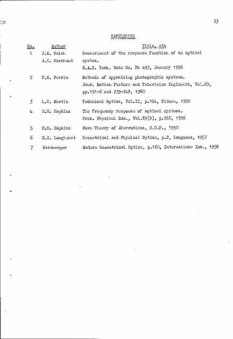
PREEREA CES

No. Author Title-. etc

I J.M. Naish Measurement of the response function of an optical

A.C° Marchant system.

R.A.E. Tech. Note No. Ph 493, January 1956

2 F.H. Perrin Methods of appraising photographic systems.

Jour. Motion Picture and Television Engineers, Vol.69,

pp.151- 6 and 239-248, 1960

3 L.C. Martin Technical Optics, Vol.II, p.104, Pitman, 1950

4 H.H. Hopkins The frequency response of optical systems.

Proc. Physical Soc., Vol.69(B), p.5 6 2, 1956

5 H.H. Hopkins Wave Theory of Aberrations, 0.U.P., 1950

6 R.S. Longhurst Geometrical and Physical Optics, p.2, Longmans, 1957

7 Herzberger Miodern Geometrical Optics, p.120, Interscience Inc., 1958

l EE 0027 Fig.1

,N,,T "oo-A MPLITUVE

DISTANCE -

FIG. I OPTICAL "SIGNAL"

Fig.2 IEE &rZS

I.r

I.0

x I..I.o

I.<w~

L7.

I EE ror Z Fig.3

Z i

z~ x

00I

< w.

TETIIOL IBAUBI-331

A31RDrEl pg IIGG0USTAPT

Fig.4 lEE 063o

FIG. 4 (a a b) EFFECTIVE PUPIL AREAS

I CE:Fig.5

w0D

6-J

ILL

0 U-00

0

z0

Kw

H w

LL

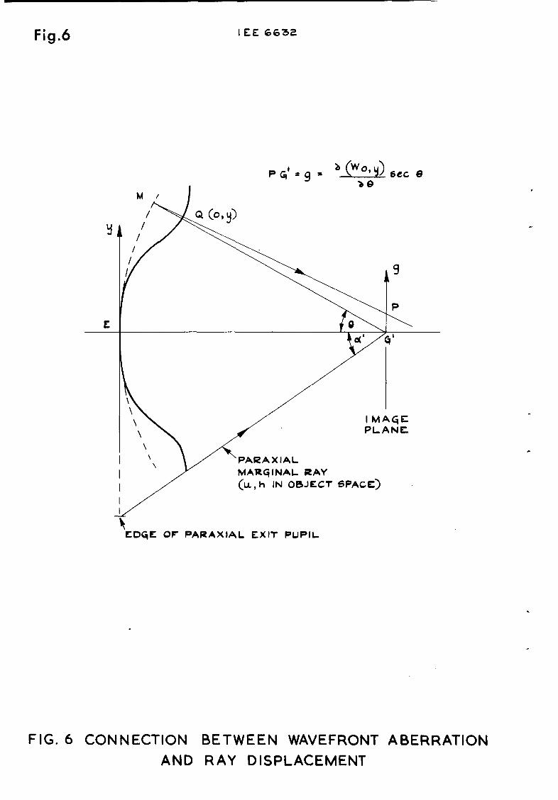
Fig.6 IEE Go612

pe 9 "(WO')sec G

M/

CL(0

I MA(qE.PLANE.

PARAXIALMAItiqINAL RAY(I.,h IN OBJECT SPACE)

EDrOE OF PARAXIAL EXIT PUPIL

FIG. 6 CONNECTION BETWEEN WAVEFRONT ABERRATION

AND RAY DISPLACEMENT

I,=z•8•,Fig.7

FIG. 7 METHOD OF DEFINING EXIT PUPIL

Fig.8 IEE Cor34

z4www

w

0 cr

0~~J 0

a.:wMr

xLi-0z0

zLi-

wLi-

zIn<

10 0-

o 00

6 OD

I EE G3s Fig.9

STOP PLANEREC-41TCRt cqLAE,

F -__A_

SURFACE CURVATURE SEPARATIONS CLEAR n n -n n4- nDIAM. dC d A'd

(mm'x 1O0) (mm) (mm ) (x I011) (x 103')I 0 0

I 4 5370 11 ".-22"747 1"71991 3"43 -9'22

S - 3.5G58 .118z6"499 1-613.29 .3'31 -8'88

3 0"8484 106.041'256 I 0 0

4 -3.6Z17 7 9.417. 297 162130 4.05 -10"45

5 4-8314- 67.8" 000 1 0 0

6 (OTOP) 0 88-0*355954 I 0 0

7 -0'4702 93'66-174 1.61342 3"31 -8686

8 4-6535 106"4P..6"191 172078 5-1 -9'17

9 -4"1482 106"4509 I160 I 0 0

S6"35 4 1'5230 P-'I2 -5.81II j \qLABB/ 0 .457./

1 0 0

A* 6TOP SETTINq FOR F15.C

FIG. 9 EXAMPLE OF LENS DESIGN DATA

(24" F/S'6 -B.P 954585: C.G. WYNNE/ N.R.D.C)

Ci.i

11

C)) 0

0d 0

c- E-4 '-. 00

m. -3 OR c

C, 5-. 0 0

-Pl 0800 C; 0 o 0'

43

'4.

0

4-)

Q) a)

4.30

a004.

r i - l

4JI4.3j

L-3

0 14

co 00 co. r-m R -

CC * N)D 0F % 0 m N N i

(0, o- C) i 0i 0-: 0 n%0& 38 3C- 1

FIG.11 RESULTS FROM PROGRJBAME A

24 in. F/5.6 (Man, Data)

Wavelength (0) = 5.8760, -4Wavelength (1) = 5.4610, -4-Wavelength (2) = 7.6820, -4

Reduced height of exit pupil = 1.00

Axis abn. coeffts.

(1) (0) (2)W(2,o) 1.5821, 0 00000, 0 -7,4008, 0w(4, ) 5.1641, 0 5.5842, 0 5.7077, 0W(6,O) -4.7360, 0 -4.2997, 0 -3-0943, 0

Exit pupil scale ratio = 0.9841

Field angle = 12.00 degrees.

Pupil shape

Q S X Y

1 7 0.00 0.762 7 0.18 0.733 7 0.35 o.694 7 0.52 0.625 7 0.67 0.516 7 0.81 0.377 7 0.92 0.208 3

467 1.00 -0.00

9 3 0o93 -0.2010 3 0.81 -0o3811 3 0.67 -0.5112 3 0.52 -0.6213 1

3 0.35 -0.6914 1

3 0.18 -0.7415 1

3 0.00 -0o75

Aberrn. coeffts,

(I) (0) (2)w(i,) 9.3080, -3 1.5099, -1 6.0239, -Iw(2, O) 4.9354, 0 3.4798, 0 -4.0567, 0W(2,2) -4.1933, 0 -3°9636, 0 -3.4744, 0V(3,I ) 2.2565, 0 1.9996, 0 1.4068, 0W(3,3) -1.0080, 0 -9,1831, -1 -6.5926, -1w(4,O) 3.34"7, 0 3.9271, 0 4.5065, 0W(4,2) 2.0455, 0 2.0085, 0 1.7253, 0W(5,1) -1 .1850, 0 -1 ,1407, 0 -9.4684, -1v(6,0) -5.1869, 0 -4.7174, 0 -3.4134, 0

FIG.1 2 DATA FOR PROG-RAMME B(9-planations in brackets)

Blank tape

I [System no.]

15 [No. of points defining pupilperipher (Fig.7)]

0.089285 [Numerical aperture in image space]

5876 [Wavelength in Angstr'6ms]

0.263 [Spatial Frequency s]

5.5842 [•, from Prog. A results: Axis Abn.

Coeffts.]

-1,2997 [W.9 0 from Prog. A results: Axis Abn.

Coeffts.]

-3.44 [w 2 , 0 corresponding to focal plane

nearest lens]

3.44 [W 2 ,0 corresponding to focal plane

farthest from lens]

0.314 [Interval AW2 ,0 between focal planes]

*• [Asterisk]

FIG. 13 RESULTS FROM PRO GRAIVIHE B

Freq. response B.

Freq. response curves

System I

Axial calculation

Tests for best focal plane

Wavelength = 5876

Azimuth (0)

s = 0.26*

S /A = 0.84

w(6,o) = -4.30 , w(4,o) 5.58w(2,0) T(s,O)-3.44 -0.00-3.10 0.15-2.75 0.33-2.41 0.49-2.06 0,60-1.72 0.61-1.38 0.52-1.03 o.36-0.69 0.19-0.34 0o06-0.00 0.010.34 0.040.69 0.101,03 0.141.38 0,131.72 0.062.06 -0.012.41 -0.062.75 -0.053.10 -0.013.44 0.04

• (40 Q/mm)

FIG. 14 DATA FOR PROG I~jý,E F(Explanations in brackets)

Blank tape

24 in. F/5.6, Field angle = 12, Best Focus•

Blank tape

15 [No. of points defining pupil periphery]

0 0.76O.18 0.73 Coordinates of0,35 0.69ciulr xil ul-0.52 o.62 0 10.67 0.51 0.220.81 0.37 0.43 0.97092 0,20.43 .91 00 -Coordinates of 0.62 0.781 0 F

0.93 -0.20 Lpupil periphery.' 0.78 o.62

0.81 -0,38 0.90 0-43

0.67 -0.51 0.97 0022

0.52 -0.62 1 00.35 -0, 69 0.97 -0.22

0.18 -0,74 0.90 -0.430.78 -0.620 -0.75 0.62 -0.78

5876 - [Wavelength - Angstr~m units] 0.43 -0.90

0-15099 0.22 -0,97-1.87000 0 -1

-3.963601. 99960

-0.91831 [Aberration coeffts,]3.927102. 00850

-1.14070-4.71740

0 [Initial value of s]

0.526 [Final value of s]

0.0526 [Interval between successive values of s]

90 [Azimuth angle in degrees]

[Asterisk]

STitle must be terminated by Carriage Return, Line Feed.

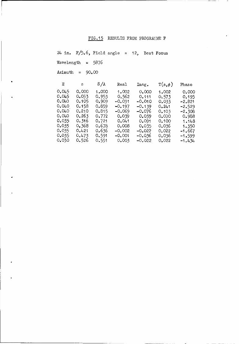
FIG. 15 RESULTS FROM PROGiMIME F

"24 in. F/5.6, Field angle = 12, Best Focus

Wavelength = 5876

Azimuth = 90.00

E S /A Real Imag. T(s,O) Phase

0.045 0.000 1.000 1.002 0.000 1.002 0.0000.045 0.053 0.953 0.562 0.111 0.573 0.1950.040 0.105 0,909 -0.031 -0.010 0.033 -2.8210.040 0.158 0.859 -0.197 -0.139 0.241 -2.5290.040 0.210 0.815 -0.069 -0.076 0.103 -2.3080.040 0.263 0.772 0.039 0.059 0.070 0.9880.035 0.316 0.721 0.041 0.091 0.100 1.1480.035 0.368 0.678 0.008 0.035 0.036 1.3500.035 0.421 0.636 -0.002 -0.022 0.022 -1.6670.035 0.473 0.591 -0.001 -0.036 0.036 -1.5990.030 0.526 0.551 0.003 -0.022 0.022 -1.434

IIE G6e6e Fig.16

- - PIRF•CT LENS

CONTRAST

0'0

0.4

0 .2 " ' "_" 18 0 0

II Io 20 40o60 60s t./,mm0 025 0.5

CALCULATION -... MEASUREMENT

(a) ON AXIS

0.8- -ISO*6

CONTRAST PHASE

0.60

0-4 - I I\ I I I\I I I

0 '2 - L _ • . -180-\ / ..... m~~ADIAL-,,, ,,.

S\/ \ .--.--

0... ---j TAN-GENTIAL0 20 40 60 8GO /m0

*(b) 120 OFF-AXIS

FIG.16(a&b) TYPICAL RESULTS(24"F/5"6 LENS: X=5876 )

DETACHABLE ABSTRACT CARDS

I~.4

-n Or, - 3 3

t aN

43~4 -

40 .4

316i

3 , 00 4

Cd)

41 0- -4

31 0 ".4 A 0