February 21, 2018

CS 361: Probability & Statistics

Random variables

Continuous probability

Continuous random variables

❖ Some quantities we would like to model don’t fit into any of the probability theory we have discussed so far: things like height, weight, temperature are all quantities that we can think of as appearing in one experimental setup or another

❖ It’s a bit tricky to formally think about sample spaces and events with these kinds of experiments and we won’t do so in this course

Continuous random variables❖ Instead, we will think of each continuous random variable

as being associated with a function p(x) called a probability density function, which we can use to do everything we would normally do with a random variable

❖ Roughly, if p(x) is a probability density function then for an infinitesimally small interval dx

❖ So in order to be a density function, p(x) must be non-negative

Probability density functions❖ Now if p(x) is the density function for some continuous

random variable and

❖ We can compute for a < b

❖ Observe, then, that

Density functions: summary❖ Density functions are non-negative

❖ (Density functions can take on values greater than 1)

❖ Integrating density functions allows us to compute the probability that a continuous random variable takes on a value within a range

❖ p(x) is not the probability that X=x

❖ Density functions integrate to 1 if we let x run from negative infinity to infinity

Density functions❖ Non-negative functions which integrate to 1 are the density

functions of some continuous random variable

❖ A continuous random variable X can be associated to a non-negative function which integrates to 1 that we can use to compute probabilities for X

❖ If we have a density for a variable, great, we can compute probabilities

❖ Many times, we are trying to come up with a sensible density to describe a continuous phenomenon

Coming up with a density functionIf instead of a density function, we have just a regular non-negative function whose shape we like, we may be able to turn it into a density function. Let f be our non-negative function that isn’t a density (it also needs to have a finite infinite integral). Then if we multiply f by a constant of proportionality it is possible to turn it into a density function. We want to find some c such that

Solving this we would get

Or that p is a density with

Example - constant of proportionalitySuppose we have a physical system that produces random numbers in the range 0 to with

No number outside this range can appear, but every number within this range is equally likely.

If X is a random variable that tells us which number was generated, what is its density function?

Recall our interpretation of the density function

We are going to want p(x) to be 0 when x < 0 or x >

We will also want p(x) to have the same value, c, for every other x since we want all outcomes in our range to be equally likely

Example - constant of proportionality

In order to figure out what c should be, recall that we must have

But

So we wind up with

Observe that we can have p(x) > 1 if

Expectation❖ With continuous variables, we compute expectations

with an integral

Expectation

This integral may not be defined or may not be finite. The cases we encounter will have well-behaved expectations, however

Useful probability distributions

Why study distributionsIt’s worth looking at certain broad families of random variables and their distributions because these families pop up a lot in practice.

And doing so allows us to construct models that can answer many questions:

What process produced the data we see? Or what can the data we observe tell us about the underlying probabilities?

What kind of data can we expect in the future?

How should we label unlabelled data? If we have a bunch of financial transactions labelled as fraudulent and legitimate, how confidently can we label a new unlabelled transaction?

Is something we are observing an interesting effect or explainable as just random noise?

Bernoulli random variablesBernoulli random variables can take on two values: 0 and 1. Good for modeling an experiment which succeeds or fails or otherwise has only two kinds of interesting outcomes.

We’ve derived the expectation and variance before

E[X] = p Var[X] = p(1-p)

Bernoulli distribution

Bernoulli random variables are a family of random variables. Each value of p is a different member of this family, but we can say general things about any member of the family, which is a major motivation for studying families of random variables

Geometric random variablesIf we have a biased coin where P(H) = p and we flip this coin again and again and stop the first time we observe heads, the number of flips required is a discrete random variable taking integer values greater than or equal to 1

To think of what the form of the distribution of this variable is, consider that it requires us to get n-1 tails each with probability 1-p and then one head with probability p. So we have

Expectation and variance

Distributionp is a called parameter

of the distribution

In homework, geometric series, hence the name

Geometric random variables

❖ Not really just about coins

❖ It can work for any situation where we have trials characterized by success and failure

❖ In some cases we want to see how to model the number of successes until a failure

❖ Or we may flip the logic and wish to model the number of failures until a success finally occurs

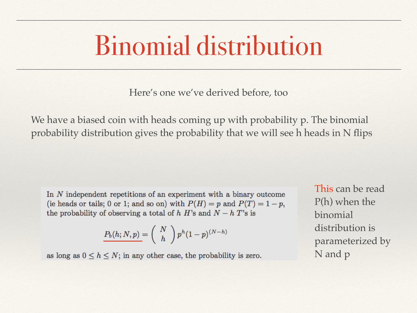
Binomial distributionHere’s one we’ve derived before, too

We have a biased coin with heads coming up with probability p. The binomial probability distribution gives the probability that we will see h heads in N flips

This can be read P(h) when the binomial distribution is parameterized by N and p

Binomial theorem and distributionWhen we did the overbooking example, someone pointed out how the distribution function of the binomial random variable looked a bit like the binomial theorem. In case you don’t remember:

Binomial Theorem x=1-py=pn=N

= 1

So our binomial distribution sums to 1 if we add P(X=h) for every which it must to satisfy our probability laws

P_b(X=k; N, p)

Binomial distribution: recursive

It’s also worth noting that our binomial distribution can be written recursively

We can get h heads in N trials by:

Getting heads on the Nth trial and then getting h-1 heads on the other N-1 trials

Getting tails on the Nth trial and getting all h heads in the other N-1 trials

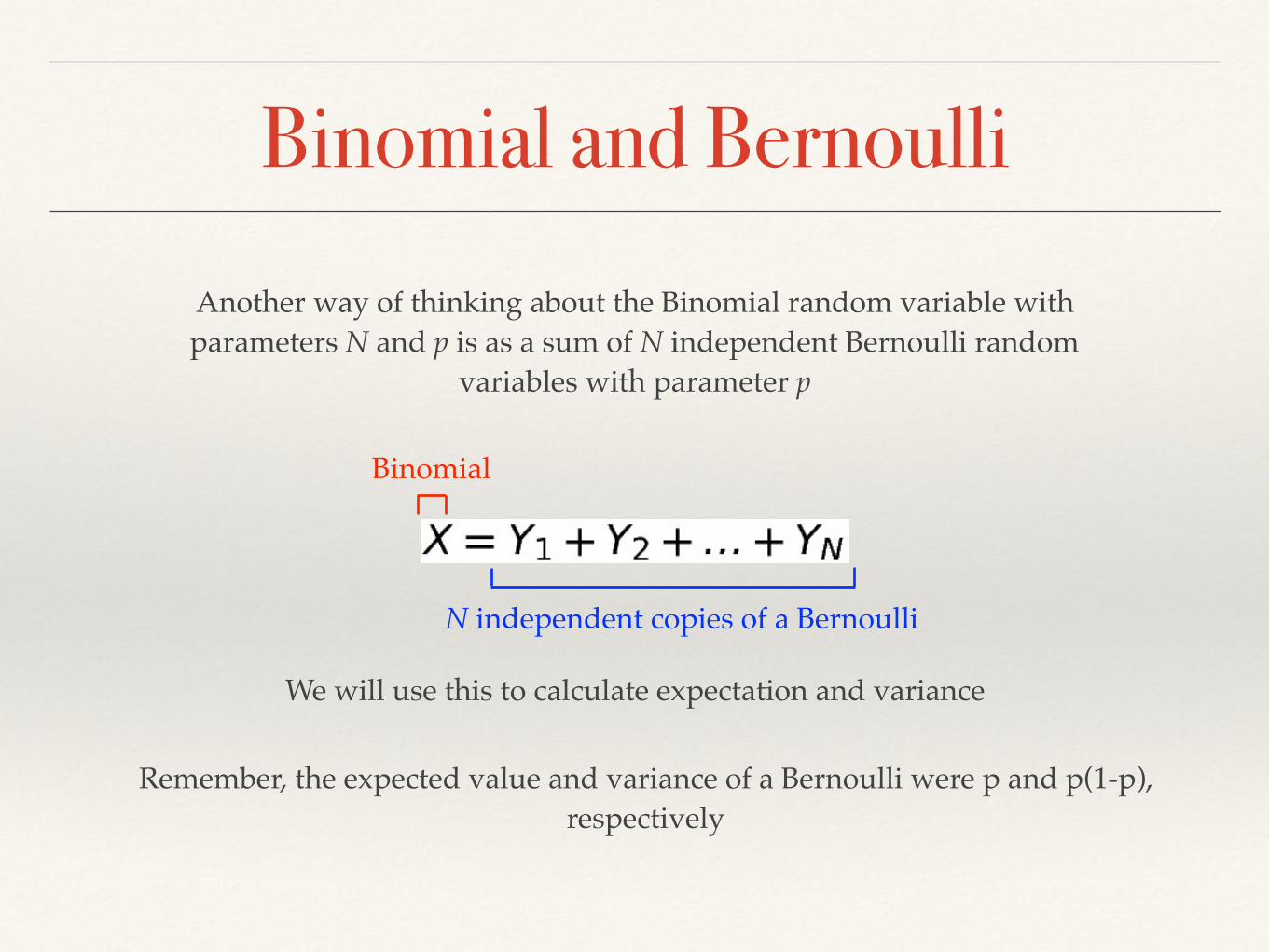
Binomial and BernoulliAnother way of thinking about the Binomial random variable with parameters N and p is as a sum of N independent Bernoulli random

variables with parameter p

We will use this to calculate expectation and variance

Binomial

N independent copies of a Bernoulli

Remember, the expected value and variance of a Bernoulli were p and p(1-p), respectively

Binomial expectationClaim:The expected value of a binomial random variable, X, with parameters N and p is Np

Let be the Bernoulli random variable associated with the i-th coin toss (recall Bernoulli is 1 when heads comes up and 0 otherwise and is parameterized by p) so that

Proof

thenThus

Using linearity

But E[Y_i] = p, so

Binomial varianceClaim:The variance of a binomial random variable with parameters N and p is Np(1-p)

Let be the Bernoulli random variable associated with the i-th coin toss (recall Bernoulli is 1 when heads comes up and 0 otherwise and is parameterized by p) so that

Same trick as before

And since these coin tosses are independent

var[Y_i] was p(1-p) so we have

Giving, as desired

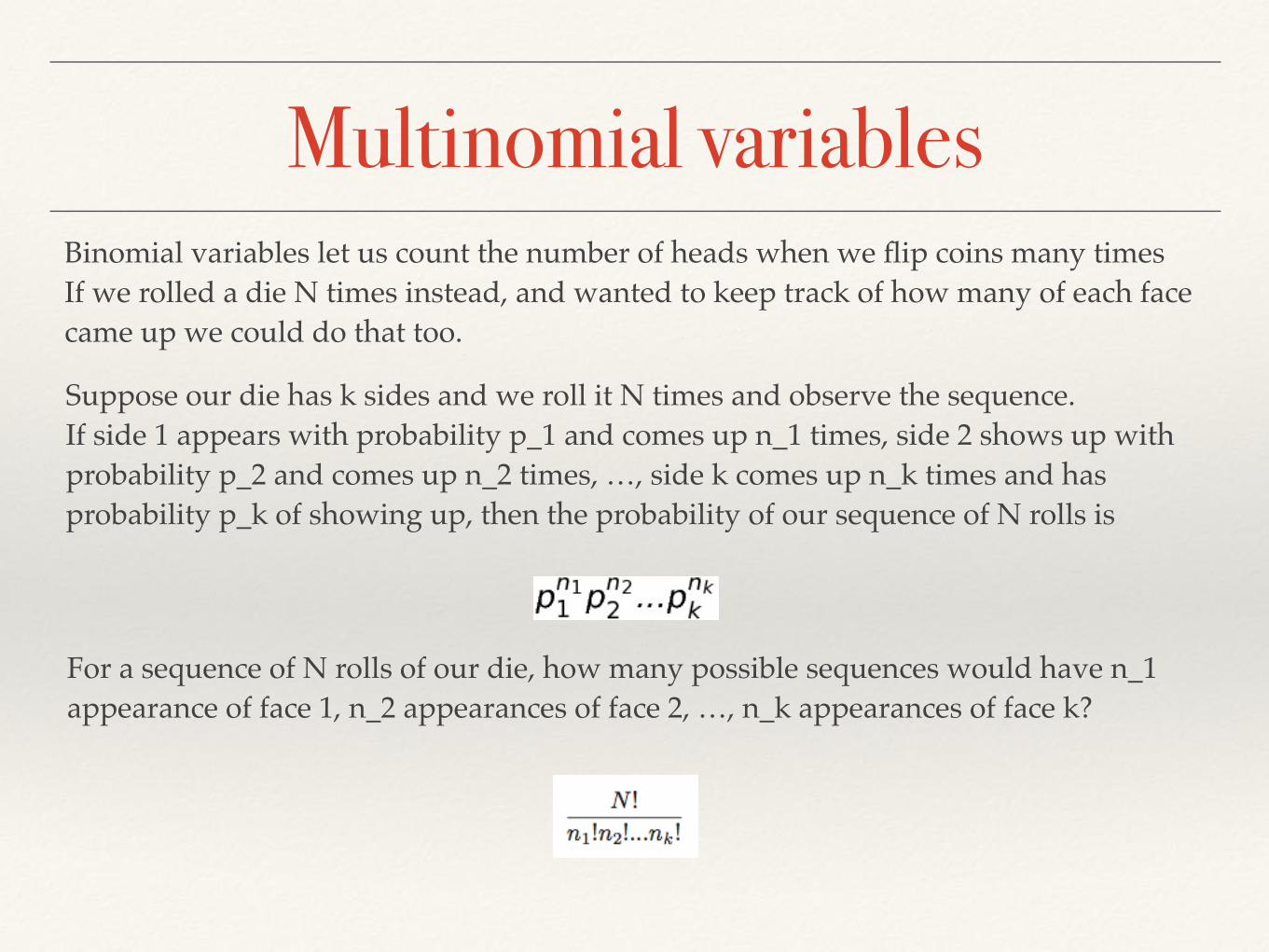
Multinomial variablesBinomial variables let us count the number of heads when we flip coins many timesIf we rolled a die N times instead, and wanted to keep track of how many of each face came up we could do that too.

Suppose our die has k sides and we roll it N times and observe the sequence. If side 1 appears with probability p_1 and comes up n_1 times, side 2 shows up with probability p_2 and comes up n_2 times, …, side k comes up n_k times and has probability p_k of showing up, then the probability of our sequence of N rolls is

For a sequence of N rolls of our die, how many possible sequences would have n_1 appearance of face 1, n_2 appearances of face 2, …, n_k appearances of face k?

Multinomial variablesWe put these two together to get the multinomial distribution. It tell us the probability if we roll a die N times, with what probability will see exactly n_1 of face 1, n_2 of face 2, …, and n_k of face k given that the die has probability p_1 of rolling a face 1, p_2 of rolling face 2, …, p_k of rolling face k. Or if we write it out

Observe that the sum of all the n_i must be N and the sum of the p_j is 1

N and the p_j are the parameters of the distribution and it is a probability distribution over k-tuples

Example: multinomial

I throw five fair dice. What is the probability of getting two 2’s and three 3’s?

The discrete uniform distributionIf every value of a discrete random variable has the same probability, then its distribution is called a discrete uniform distribution

We’ve used this in a number of examples: heads 1, tails 0 with a fair coin. Rolling a fair die, etc.

If there are N possible values, P(X=x) = 1/N if x is one of the allowable values