fault-tolerant and secure control systems · acknowledgments these notes are for the graduate...
TRANSCRIPT

Fault-Tolerant and Secure
Control Systems
Shreyas Sundaram
Department of Electrical and Computer Engineering
University of Waterloo

Acknowledgments
These notes are for the graduate course on Fault-Tolerant and Secure Control Systemsoffered at the University of Waterloo. They are works in progress, and will be continuallyupdated and corrected.
The LATEX template for The Not So Short Introduction to LATEX2ε by T. Oetiker et al.was used to typeset portions of these notes.
Shreyas SundaramUniversity of Waterloo
c© Shreyas Sundaram

Contents
1 Introduction 1
1.1 Dynamical Systems and Control Theory . . . . . . . . . . . . . . . . . . . 2
1.2 Overview of Fault-Tolerance and Security . . . . . . . . . . . . . . . . . . 4
1.2.1 Fault Detection . . . . . . . . . . . . . . . . . . . . . . . . . . . . . 5
1.2.2 Fault Accommodation . . . . . . . . . . . . . . . . . . . . . . . . . 6
1.3 What is Covered in This Course? . . . . . . . . . . . . . . . . . . . . . . . 7
2 Linear System Theory 8
2.1 Discrete-Time Signals . . . . . . . . . . . . . . . . . . . . . . . . . . . . . 8
2.2 Linear Time-Invariant Systems . . . . . . . . . . . . . . . . . . . . . . . . 9
2.3 Mathematical Models . . . . . . . . . . . . . . . . . . . . . . . . . . . . . 9
2.3.1 A Simple Model for a Car . . . . . . . . . . . . . . . . . . . . . . . 10
2.3.2 Longitudinal Dynamics of an F-8 Aircraft . . . . . . . . . . . . . . 11
2.3.3 Linear Feedback Shift Register . . . . . . . . . . . . . . . . . . . . 12
2.4 State-Space Models . . . . . . . . . . . . . . . . . . . . . . . . . . . . . . . 13
2.4.1 Transfer Functions of Linear State-Space Models . . . . . . . . . . 14
2.4.2 State-Space Realizations and Similarity Transformations . . . . . . 15
2.5 Stability of Linear Systems . . . . . . . . . . . . . . . . . . . . . . . . . . 16
2.6 Properties of Linear Systems . . . . . . . . . . . . . . . . . . . . . . . . . 17
2.6.1 Controllability . . . . . . . . . . . . . . . . . . . . . . . . . . . . . 17
2.6.2 Observability . . . . . . . . . . . . . . . . . . . . . . . . . . . . . . 19
2.6.3 Invertibility . . . . . . . . . . . . . . . . . . . . . . . . . . . . . . . 21
2.6.4 Strong Observability . . . . . . . . . . . . . . . . . . . . . . . . . . 24
2.6.5 System Properties and Similarity Transformations . . . . . . . . . 27
c© Shreyas Sundaram

CONTENTS iv
2.7 State-Feedback Control . . . . . . . . . . . . . . . . . . . . . . . . . . . . 29
2.8 State Estimators and Observer Feedback . . . . . . . . . . . . . . . . . . . 30
2.8.1 State Estimator Design . . . . . . . . . . . . . . . . . . . . . . . . 31
2.8.2 The Separation Principle . . . . . . . . . . . . . . . . . . . . . . . 32
2.9 Matrix Pencil Characterizations of System Properties . . . . . . . . . . . 33
2.9.1 Controllability and Observability . . . . . . . . . . . . . . . . . . . 34
2.9.2 Invertibility . . . . . . . . . . . . . . . . . . . . . . . . . . . . . . . 35
2.9.3 Strong Observability . . . . . . . . . . . . . . . . . . . . . . . . . . 36
3 Observers for Linear Systems with Unknown Inputs 39
3.1 Unknown Input Observer . . . . . . . . . . . . . . . . . . . . . . . . . . . 39
3.2 Design Procedure . . . . . . . . . . . . . . . . . . . . . . . . . . . . . . . . 42
3.3 Relationship to Strong Detectability . . . . . . . . . . . . . . . . . . . . . 43
4 Fault-Detection and Isolation Schemes 48
4.1 Sensor Fault Detection . . . . . . . . . . . . . . . . . . . . . . . . . . . . . 48
4.2 Robust Fault Detection and Identification . . . . . . . . . . . . . . . . . . 50
4.2.1 Fault Detection: Single Observer Scheme . . . . . . . . . . . . . . 51
4.2.2 Single Fault Identification: Bank of Observers . . . . . . . . . . . . 53
4.2.3 Multiple Fault Identification: Dedicated Observers . . . . . . . . . 54
4.3 Parity Space Methods . . . . . . . . . . . . . . . . . . . . . . . . . . . . . 55
5 Reliable System Design 58
5.1 Majority Voting with Unreliable Components . . . . . . . . . . . . . . . . 58
5.2 A Coding-Theory Approach to Reliable Controller Design . . . . . . . . . 62
5.2.1 Background on Parity-Check Codes . . . . . . . . . . . . . . . . . 62
5.2.2 Reliable Controller Design . . . . . . . . . . . . . . . . . . . . . . . 66
6 Control Over Packet-Dropping Channels 74
6.1 Control of a Scalar System with Packet Drops . . . . . . . . . . . . . . . . 75
6.2 General Linear Systems with Packet Drops . . . . . . . . . . . . . . . . . 76
6.2.1 Lyapunov Stability of Linear Systems . . . . . . . . . . . . . . . . 77
6.2.2 Mean Square Stability of Linear Systems with Packet Drops . . . . 80
c© Shreyas Sundaram

CONTENTS v
7 Information Dissemination in Distributed Systems and Networks 84
7.1 Distributed System Model . . . . . . . . . . . . . . . . . . . . . . . . . . . 86
7.2 Linear Iterative Strategies for Asymptotic Consensus . . . . . . . . . . . . 86
7.2.1 Choosing the Weight Matrix for Asymptotic Consensus . . . . . . 89
7.2.2 Notes on Terminology . . . . . . . . . . . . . . . . . . . . . . . . . 91
7.3 Linear Iterative Strategies for Secure Data Aggregation . . . . . . . . . . 92
7.3.1 Attacking the Network . . . . . . . . . . . . . . . . . . . . . . . . . 93
7.3.2 Modeling Malicious Nodes in the Linear Iterative Strategy . . . . . 94
7.3.3 Calculating Functions in the Presence of Malicious Nodes whenκ ≥ 2f + 1 . . . . . . . . . . . . . . . . . . . . . . . . . . . . . . . 96
A Linear Algebra 102
A.1 Fields . . . . . . . . . . . . . . . . . . . . . . . . . . . . . . . . . . . . . . 102
A.2 Vector Spaces and Subspaces . . . . . . . . . . . . . . . . . . . . . . . . . 103
A.3 Linear Independence and Bases . . . . . . . . . . . . . . . . . . . . . . . . 104
A.4 Matrices . . . . . . . . . . . . . . . . . . . . . . . . . . . . . . . . . . . . . 105
A.4.1 Linear transformations, Range space and Null Space . . . . . . . . 106
A.4.2 Systems of Linear Equations . . . . . . . . . . . . . . . . . . . . . 108
A.4.3 Determinants . . . . . . . . . . . . . . . . . . . . . . . . . . . . . . 109
A.4.4 Eigenvalues and Eigenvectors . . . . . . . . . . . . . . . . . . . . . 110
A.4.5 Similarity Transformations, Diagonal and Jordan Forms . . . . . . 114
A.4.6 Symmetric and Definite Matrices . . . . . . . . . . . . . . . . . . . 116
A.4.7 Vector Norms . . . . . . . . . . . . . . . . . . . . . . . . . . . . . . 119
B Graph Theory 121
B.1 Paths and Connectivity . . . . . . . . . . . . . . . . . . . . . . . . . . . . 122
B.2 Matrix Representations of Graphs . . . . . . . . . . . . . . . . . . . . . . 124
C Structured System Theory 127
C.1 Structured Systems . . . . . . . . . . . . . . . . . . . . . . . . . . . . . . . 127
C.2 Graphical Test for Nonsingularity . . . . . . . . . . . . . . . . . . . . . . . 130
C.3 Structural Properties of Linear Systems . . . . . . . . . . . . . . . . . . . 133
C.3.1 Generic Rank of the Matrix Pencil . . . . . . . . . . . . . . . . . . 133
C.3.2 Structural Controllability . . . . . . . . . . . . . . . . . . . . . . . 136
c© Shreyas Sundaram

CONTENTS vi
C.3.3 Structural Observability . . . . . . . . . . . . . . . . . . . . . . . . 139
C.3.4 Structural Invertibility . . . . . . . . . . . . . . . . . . . . . . . . . 139
C.3.5 Structural Invariant Zeros . . . . . . . . . . . . . . . . . . . . . . . 140
c© Shreyas Sundaram

Chapter 1
Introduction
The world around us is replete with complex engineered systems: automobiles [11], airtraffic control systems [54], building energy management systems [88], industrial processsystems [79], and the electrical power grid [58] are just a few examples. Many of thesesystems are life- and mission-critical, where disruptions (either by intent or by accident)could have dire consequences. There have been various incidents in recent years thatexemplify this fact [27, 50, 81].
• In 1999, a gas pipeline belonging to Olympic Pipeline Co exploded, killing threepeople. One of the many factors that led to this explosion was that the supervisorycontrol system became unresponsive and failed to take action to relieve the buildupof pressure in the pipeline. The reason for this failure was later determined to becaused by an update of the control system software just before the incident tookplace, without adequate testing in an offline environment [7].
• In 2000, a disgruntled employee hacked into the control system responsible formanaging the sewage system in Queensland, Australia, causing it to release 264, 000tons of sewage into parks and rivers [80].
• In 2003, an overloaded transmission line in Ohio tripped, starting a chain of cas-cading failures. Around the same time, the monitoring systems at power controlrooms failed, leading operators to miss the alarms. Within hours, a large portionof the Northeastern United States and Canada were affected by a major powerfailure, affecting more than 50 million people.
In addition to the above high-profile incidents, faults can have a detrimental impacton low-profile day-to-day activities. For example, modern high-performance buildingsare typically designed to operate efficiently and minimize energy usage via the use ofmany sensors and advanced control strategies. However, the intended gains will not berealized if the sensors or control systems fail, leading to energy waste and uncomfortableconditions [43, 45].
c© Shreyas Sundaram

1.1 Dynamical Systems and Control Theory 2
To avoid physical and economic damage caused by such incidents, it is imperative to de-sign systems to be resilient to unexpected events. Much work has been done over the pastfew decades on developing mechanisms for obtaining fault-tolerance in different types ofsystems. These range from conceptually simple modular redundancy schemes to moreadvanced model-based fault-diagnosis techniques. The need for a rigorous theory of secu-rity in control systems has only recently been recognized as a fertile and important areaof research. The report [81] highlights several key differences in security requirementsfor control systems and traditional information technology systems. One particularlyimportant differentiating factor is that control systems involve the regulation of physicalprocesses. This fact imposes hard real-time constraints on the system, since a delay inprocessing could lead to instabilities or cascading failures in the control loop, poten-tially causing severe physical and economic damage. Information technology systems,on the other hand, focus on the protection and delivery of data as the key priority; whiledelays or down-time are highly undesirable, they can frequently be tolerated withoutcausing major or permanent damage. The paper [9] echoes the call for the developmentof a rigorous theory of security in control systems, detailing several open challenges forresearch. Furthermore, the North American Electric Reliability Corporation (NERC)and the US Department of Energy have mandated that electric utilities comply withstrict cyber-security standards, and are turning down smart power grid projects thatdo not incorporate such measures in their design [52, 33]. However, ensuring securityand reliability in these cases poses a unique challenge; the complex interplay of control,communications and computation in such systems necessitates a holistic approach todesign.
At a philosophical level, one can view attacks as a type of ‘worst-case’ fault, wherethe location and magnitude of the fault are chosen so as to cause the most damageto the system. In this course, we will be adopting this perspective, and developing amethodology to deal with faults and attacks using rigorous mathematical tools. We willbe focusing on a particular class of systems that involve dynamics, which we will describenext.
1.1 Dynamical Systems and Control Theory
For the purposes of this course, a system is an abstract object that accepts inputs andproduces outputs in response. Systems are often composed of smaller components thatare interconnected together, leading to behavior that is more than just the sum of itsparts. In the control literature, systems are also commonly referred to as plants orprocesses.
SystemInput Output
Figure 1.1: An abstract representation of a system.
c© Shreyas Sundaram
1.1 Dynamical Systems and Control Theory 3
The term dynamical system loosely refers to any system that has a state and somedynamics (i.e., a rule specifying how the state evolves in time). This description applies toa very large class of systems, from automobiles and aviation to industrial manufacturingplants and the electrical power grid. The presence of dynamics implies that the behaviorof the system cannot be entirely arbitrary; the temporal behavior of the system’s stateand outputs can be predicted to some extent by an appropriate model of the system.
In physical systems, the inputs are applied via actuators, and the outputs are measure-ments of the system state provided by sensors.
Example 1.1. Consider a simple model of a car in motion, and let the speed of the carat any time t be given by v(t). One of the inputs to the system is the acceleration a(t),applied by the throttle (the actuator). Suppose that we are interested in the speed ofthe car at every second (i.e., at t = 0, 1, 2, . . .), and that the acceleration of the car onlychanges every second, and is held constant in between changes. We can then write
v(t+ 1) = v(t) + a(t), (1.1)
since the speed of the car one second from now is just the current speed plus the acceler-ation during that second. The quantity v(t) is the state of the system, and equation (1.1)specifies the dynamics. There is a speedometer on the car, which is a sensor that measuresthe speed once per second. The value provided by the sensor is denoted by s(t) = v(t),and this is taken to be the output of the system.
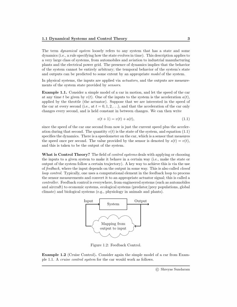
What is Control Theory? The field of control systems deals with applying or choosingthe inputs to a given system to make it behave in a certain way (i.e., make the state oroutput of the system follow a certain trajectory). A key way to achieve this is via the useof feedback, where the input depends on the output in some way. This is also called closedloop control. Typically, one uses a computational element in the feedback loop to processthe sensor measurements and convert it to an appropriate actuator signal; this is called acontroller. Feedback control is everywhere, from engineered systems (such as automobilesand aircraft) to economic systems, ecological systems (predator/prey populations, globalclimate) and biological systems (e.g., physiology in animals and plants).
SystemOutput
Mapping fromoutput to input
Input
Figure 1.2: Feedback Control.
Example 1.2 (Cruise Control). Consider again the simple model of a car from Exam-ple 1.1. A cruise control system for the car would work as follows.
c© Shreyas Sundaram

1.2 Overview of Fault-Tolerance and Security 4
Controller System
DesiredOutput
ControlInput Output
−
Figure 1.3: Block Diagram of a feedback control system.
• The speedometer in the car measures the current speed and produces s(t) = v(t).
• The controller in the car uses these measurements to produce control signals: ifthe current measurement s(t) is less than the desired cruising speed, the controllersends a signal to the throttle to accelerate, and if s(t) is greater than the desiredspeed, the throttle is asked to allow the car to slow down.
• The throttle performs the action specified by the controller.
Example 1.3 (Inverted Pendulum). Suppose we try to balance a stick vertically inthe palm of our hand. The sensor, controller and actuator in this example are oureyes, our brain, and our hand, respectively. This is an example of a feedback controlsystem. Now what happens if we try to balance the stick with our eyes closed? Thestick inevitably falls. This illustrates another type of control, known as feedforwardcontrol, where the input to the system does not depend on the output. As this exampleillustrates, feedforward control is not robust to disturbances – if the stick is not perfectlybalanced to start, or if our hand moves very slightly, the stick will fall.
Note that systems typically have many inputs, some of which are not under the controlof the designer. One common example of this is the presence of disturbances in thesystem. For example, the motion of the car might be affected by wind gusts, or mightencounter slippery road conditions. Control theory uses mathematical tools and analysisto determine the proper inputs to apply (based on the outputs of the system) in orderto obtain correct, safe and efficient behavior, despite the presence of disturbances.
1.2 Overview of Fault-Tolerance and Security
Components of systems can fail due to a variety of factors, ranging from wear-and-tear,adverse conditions, accidents, or targeted attacks. With regard to the discussion inthe previous section, faults or attacks can manifest themselves in the plant (changingthe system dynamics), sensors (providing incorrect state measurements), or actuators(applying incorrect inputs). This can cause the functioning of the system to be severelyimpacted, unless care has been taken to design fault-tolerance into the system. Thegoal of fault-tolerant control is to allow the system to gracefully degrade or continuefunctioning under failures, and prevent faults from propagating to other parts of thesystem. Fault-tolerance can broadly be broken down into two objectives [6]:
c© Shreyas Sundaram

1.2 Overview of Fault-Tolerance and Security 5
1. Fault detection and identification (FDI): determine whether a fault has oc-curred, and isolate the component that has failed.
2. Fault accommodation: take steps to correct for the fault, or reconfigure yoursystem to avoid the faulty component.
Figure 1.4 shows a block diagram from [6] that illustrates the structure of a fault-tolerantcontrol system.
Figure 1.4: A fault-tolerant control system [6].
1.2.1 Fault Detection
To perform fault-detection, one compares the actual behavior of the plant to expectedbehavior, and raises an alarm if the two deviate. The expected behavior is usuallydetermined from a model of the plant; when there are disturbances or the model isuncertain, the expected and actual outputs will not coincide exactly. In such cases,the control system designer must determine ‘how different’ the two signals are allowedto be before raising an alarm. There is a trade-off here: if the threshold is set toolow, there will be many false alarms, and if the threshold is too high, some legitimatefaults might be missed. The relative weighting of these two factors will depend on theapplication at hand. It is important to note that the above scheme is a real-time faultmonitoring system, in that it runs concurrently with the system. This is in contrast toscheduled fault-diagnosis, where the system is checked at regular intervals according tosome maintenance schedule to ensure that it is operating correctly. Real-time monitoringis important for safety-critical systems, so that a fault does not cause the system tobecome unstable, or progress to a state where it cannot be repaired.
There are a variety of methods to perform fault-detection. The most straightforwardmethod is to use physical redundancy: the fault-prone components are replicated, anda comparison mechanism (e.g., majority voter) is used to determine which componentsare operating correctly. This scheme has the benefit of being simple to understand andimplement, but could potentially be costly due to the replication of components.
c© Shreyas Sundaram

1.2 Overview of Fault-Tolerance and Security 6
An alternative (or perhaps complementary) method to diagnose faults is to analyze thebehavior of the component over time, using a model of how the component is supposed tobehave. This is known as analytical redundancy or temporal redundancy. The followingexample (motivated by [12]) illustrates this concept.
Example 1.4. Consider again the model of the car in Example 1.1, with internal statev(t) (its speed) and dynamics given by (1.1). Now suppose that the sensor can potentiallyfail, so that it stops providing correct measurements of the speed. We would like todevelop a mechanism to diagnose this failure.
Physical Redundancy: The most obvious way to detect failures would be to installtwo sensors, each of which provides an independent measurement of the speed, i.e.,s1(t) = v(t) and s2(t) = v(t). If one of the sensors stops working, we would detect thisby noting that the two measurements do not match. If we put in a third sensor, we couldtell which sensor is malfunctioning simply by majority voting on the three sensors.
Analytical Redundancy: Instead of installing two sensors in order to detect a failure,suppose that we knew the model of the system (given by equation (1.1)), along with theacceleration input a(t). Then, if the sensor is working (i.e., s(t) = v(t)), it must be thecase that
s(t+ 1) = s(t) + a(t).
However, if the sensor is malfunctioning, this equation will (generally) not hold. Thus wewould detect a failure without duplicating the sensor, but instead by using the temporalredundancy in the sensor measurements.
The above concept can be generalized to handle dynamical systems that are characterizedby differential or difference equations (as is the case with many physical systems). Inthis course, we will show how to use linear system theory and linear algebra to treatsuch systems. By leveraging both temporal and physical redundancies, one may be ableto operate the system and diagnose faults more efficiently.
Note that when one is concerned about attacks (i.e., worst-case faults), a properly de-signed fault-detection mechanism can be used to discover the source of attacks and raisean alarm so that appropriate defensive actions can be taken.
1.2.2 Fault Accommodation
While detecting and identifying faults quickly is very important, designing the system tofunction correctly despite faults is also a prime goal. The standard technique to achievethis is again via modular redundancy: if the fault-prone components are replicated anda voter compares their outputs, the correct components will prevail as long as less thanhalf of the components are faulty. This is the approach taken in high-risk avionics such asthe space-shuttle (which uses five redundant computers) [78], and the Boeing 777 (whichuses three redundant computers, each of which consists of three internally redundantcomputing elements) [97]. Furthermore, at least one of the redundant elements in bothof these applications is designed by a different team and using different technology thanthe other elements, so that a common coding problem or design defect will not affect all
c© Shreyas Sundaram

1.3 What is Covered in This Course? 7
of the elements in the same way. While this is a simple and effective method to achievefault-tolerance, it clearly comes at a large cost due to the replication of technology anddesign effort by different teams.
In the second half of this course, we will study design techniques for control systems thatare tolerant to different types of faults or attacks. Depending on the fault models thatone is interested in, we will show how reliable control can be achieved without necessarilyresorting to a large number of redundant components or controllers.
1.3 What is Covered in This Course?
The objective of this course is to provide an overview of different techniques for con-structing reliable control systems. Due to the very broad applicability of this topic, thiscourse will not attempt to discuss every possible application. Instead, we will deal withthe underlying mathematical theory, analysis, and design of fault- and attack-tolerantsystems. Topics will include model-based techniques for fault diagnosis, graph-basedanalysis techniques for linear systems, and the application of traditional fault-tolerancetechniques to synthesizing reliable control mechanisms. The course will also cover re-cent research on the topics of tolerating packet dropouts in networked control systems,exchanging information in multi-agent systems despite the presence of malicious agents,and analyzing the vulnerability of large-scale complex systems (such as the power gridand the Internet) to attacks and failures.
The trajectory of the course will be as follows.
• Mathematical background: Before we can analyze a given system to determineits fault-tolerance properties, we will need some mathematical tools. Our primarytools will be linear algebra, linear system theory, and graph theory. We will reviewthese concepts at the start of the course.
• Fault-diagnosis: Once we have the tools from linear system theory, we can startexamining mathematical models of systems, and come up with systematic ways toanalyze their outputs in order to detect faults.
• Design: We will then study ways to design control systems that are able to main-tain proper behavior despite faults in the system. Our investigations will rangefrom classical modular redundancy techniques (such as those used in aircraft) tomore recent work on designing self-correcting controllers. We will also discuss top-ics in fault and attack-tolerant control of multi-agent systems, and time-permitting,end with a brief overview of work on studying the robustness of large-scale complexnetworks.
c© Shreyas Sundaram

Chapter 2
Linear System Theory
In this course, we will be dealing primarily with linear systems, a special class of sys-tems for which a great deal is known. During the first half of the twentieth century,linear systems were analyzed using frequency domain (e.g., Laplace and z-transform)based approaches in an effort to deal with issues such as noise and bandwidth issuesin communication systems. While they provided a great deal of intuition and were suf-ficient to establish some fundamental results, frequency domain approaches presentedvarious drawbacks when control scientists started studying more complicated systems(containing multiple inputs and outputs, nonlinearities, noise, and so forth). Starting inthe 1950’s (around the time of the space race), control engineers and scientists startedturning to state-space models of control systems in order to address some of these issues.These time-domain approaches are able to effectively represent concepts such as the in-ternal state of the system, and also present a method to introduce optimality conditionsinto the controller design procedure. We will be using the state-space (or “modern”)approach to control almost exclusively in this course, and the purpose of this chapter isto review some of the essential concepts in this area.
2.1 Discrete-Time Signals
Given a field F, a signal is a mapping from a set of numbers to F; in other words, signalsare simply functions of the set of numbers that they operate on. More specifically:
• A discrete-time signal f is a mapping from the set of integers Z to F, and is denotedby f [k] for k ∈ Z. Each instant k is also known as a time-step.
• A continuous-time signal f is a mapping from the set of real numbers R to F andis denoted by f(t) for t ∈ R.
One can obtain discrete-time signals by sampling continuous-time signals. Specifically,suppose that we are interested in the value of the signal f(t) at times t = 0, T, 2T, . . . ,
c© Shreyas Sundaram

2.2 Linear Time-Invariant Systems 9
for some positive constant T . These values form a sequence f(kT ) for k ∈ N, and if wesimply drop the constant T from the notation (for convenience), we obtain the discrete-time sequence f [k] for k ∈ N. Since much of modern control deals with sampled versionsof signals (due to the reliance on digital processing of such signals), we will be primarilyworking with discrete-time signals in this course, and focusing on the case where F = C
(the field of complex numbers).
2.2 Linear Time-Invariant Systems
Consider the system from Figure 1.1, with an input signal u and an output signal y. Thesystem is either discrete-time or continuous-time, depending on the types of the signals.In our discussion, we will focus on the discrete-time case, but the results and definitionstransfer in a straightforward manner to continuous-time systems.
In order to analyze and control the system, we will be interested in how the outputsrespond to the inputs. We will be particularly interested in systems that satisfy thefollowing property.
Definition 2.1 (Principle of Superposition). Suppose that the out-put of the system is y1[k] in response to input u1[k] and y2[k] inresponse to input u2[k]. The Principle of Superposition holds if theoutput of the system in response to the input αu1[k] + βu2[k] isαy1[k] + βy2[k], where α and β are arbitrary real numbers. Notethat this must hold for any inputs u1[k] and u2[k].
The system is said to be linear if the Principle of Superposition holds. The system issaid to be time-invariant if the output of the system is y[k − κ] when the input isu[k−κ] (i.e., a time-shifted version of the input produces an equivalent time-shift in theoutput). These concepts are illustrated in Fig. 2.1.
2.3 Mathematical Models
Mathematical models for many systems can be derived either from first principles (e.g.,using Newton’s Laws of motion for mechanical systems and Kirchoff’s voltage and currentlaws for electrical systems). As noted earlier, many physical systems are inherentlycontinuous-time, and thus their models would involve systems of differential equations.However, by sampling the system, one can essentially use discrete-time models to analyzesuch systems. In this course, we will predominantly be working with systems that canbe represented by a certain mathematical form, and not focus too much on the explicitsystem itself. In other words, we will be interested in studying general properties and
c© Shreyas Sundaram

2.3 Mathematical Models 10
Figure 2.1: (a) The Principle of Superposition. (b) The Time-Invariance Property.
analysis methods that can be applied to a variety of systems. To introduce the generalmathematical system model that we will be considering, however, it will first be usefulto consider a few examples.
2.3.1 A Simple Model for a Car
Consider again the model of the car from Chapter 1, with speed v(t) at any time t, andacceleration input a(t). Along the lines of Example 1.1, suppose that we sample thevelocity of the car every T seconds, and that the acceleration is held constant betweensampling times. We can then write
v[k + 1] = v[k] + Ta[k], (2.1)
where v[k] is shorthand for v(kT ), k ∈ N, and a[k] is the acceleration that is applied attime t = kT . Now, suppose that we wish to also consider the amount of fuel in the car atany given time-step k: let g[k] denote this amount. We can consider a very simple modelfor fuel consumption, where the fuel decreases linearly with the distance traveled. Letd[k] denote the distance traveled by the car between sampling times kT and (k + 1)T ,and recall from basic physics that under constant acceleration a[k] and initial velocityv[k], this distance is given by
d[k] = Tv[k] +T 2
2a[k].
Thus, if we let δ denote some coefficient that indicates how the fuel decreases withdistance, we can write
g[k + 1] = g[k]− δd[k] = g[k]− δT v[k]− δT 2
2a[k]. (2.2)
c© Shreyas Sundaram

2.3 Mathematical Models 11
Equations (2.1) and (2.2) together form a two-state model of a car. We can put themtogether concisely using matrix-vector notation as follows:
[v[k + 1]g[k + 1]
]
︸ ︷︷ ︸
x[k+1]
=
[1 0
−δT 1
] [v[k]g[k]
]
︸ ︷︷ ︸
x[k]
+
[T
−δ T 2
2
]
a[k] . (2.3)
The state of this system is given by the vector x[k] =[v[k] g[k]
]′, and the input is the
acceleration a[k], as before. If we consider the speedometer that provides a measurementof the speed at every sampling instant, the output of the system would be
s[k] = v[k] =[1 0
]x[k].
We could also have a fuel sensor that measures g[k] at each time-step; in this case, wewould have two outputs, given by the vector
y[k] =
[1 00 1
]
x[k],
where the first component corresponds to the sensor measurement of the speed, and thesecond component corresponds to the fuel sensor.
2.3.2 Longitudinal Dynamics of an F-8 Aircraft
Consider a model for the (sampled) linearized longitudinal dynamics of an F-8 aircraft[87]:
V [k + 1]γ[k + 1]α[k + 1]q[k + 1]
︸ ︷︷ ︸
x[k+1]
=
0.9987 −3.2178 −4.4793 −0.22200 1 0.1126 0.00570 0 0.8454 0.0897
0.0001 −0.0001 −0.8080 0.8942
V [k]γ[k]α[k]q[k]
︸ ︷︷ ︸
x[k]
+
−0.03290.0131
−0.0137−0.0092
u[k], (2.4)
where V [k] is the velocity of the aircraft, γ[k] is the flight-path angle, α[k] is the angle-of-attack, and q[k] is the pitch rate. The input to the aircraft is taken to be the deflectionof the elevator flaps.
The output of the system will depend on the sensors that are installed on the aircraft.For example, if there is a sensor to measure the velocity and the pitch rate, the outputwould be given by
y[k] =
[1 0 0 00 0 0 1
]
x[k].
c© Shreyas Sundaram

2.3 Mathematical Models 12
2.3.3 Linear Feedback Shift Register
Consider, a linear feedback shift register (LFSR), which is a digital circuit used to imple-ment functions such as random number generators and “noise” sequences in computers.
n n− 1 · · · 2 1
fu
Figure 2.2: A Linear Feedback Shift Register
The LFSR consists of n registers that are chained together. At each clock-cycle k, eachregister takes the value of the next register in the chain. The last register’s value iscomputed as a function of the values of other registers further up the chain, and perhapswith an additional input u[k]. If we denote the value stored in register i at time-step (orclock-cycle) k by xi[k], we obtain the model
x1[k + 1] = x2[k]
x2[k + 1] = x3[k]
...
xn−1[k + 1] = xn[k]
xn[k + 1] = α0x1[k] + α1x2[k] + · · ·+ αn−1xn[k] + βu[k],
(2.5)
for some scalars α0, α1, . . . , αn−1, β. These scalars and input are usually chosen so thatthe sequence of values generated by register 1 exhibits certain behavior (e.g., simulatesthe generation of a “random” sequence of values). Let y[k] = x1[k] denote the outputof the system. One can write the above equations more compactly by defining the statevector
x[k] ,[x1[k] x2[k] · · · xn[k]
]′,
from which we obtain
x[k + 1] =
0 1 0 0 · · · 00 0 1 0 · · · 00 0 0 1 · · · 0...
......
.... . .
...0 0 0 0 · · · 1α0 α1 α2 α3 · · · αn−1
︸ ︷︷ ︸
A
x[k] +
000...0β
︸︷︷︸
B
u[k]
y[k] =[1 0 0 0 · · · 0
]
︸ ︷︷ ︸
C
x[k].
c© Shreyas Sundaram

2.4 State-Space Models 13
2.4 State-Space Models
In the last section, we saw some examples of physical systems that can be modeled viaa set of discrete-time equations, which were then put into a matrix-vector form. Suchforms known as state-space models of linear systems, and can generally have multipleinputs and outputs to the system, with general system matrices.1
The state-space model for a discrete-time linear system is given by
x[k + 1] = Ax[k] +Bu[k]
y[k] = Cx[k] +Du[k] .(2.6)
The state-space model of a continuous-time linear system is givenby
x = Ax+Bu
y = Cx+Du .(2.7)
• The vector x is called the state vector of the system. We will denote the numberof states in the system by n, so that x ∈ Rn. The quantity n is often called theorder or dimension of the system.
• In general, we might have multiple inputs u1, u2, . . . , um to the system. In thiscase, we can define an input vector u =
[u1 u2 · · · um
]′.
• In general, we might have multiple outputs y1, y2, . . . , yp. In this case, we can
define the output vector y =[y1 y2 · · · yp
]′. Note that each of these outputs
represents a sensor measurement of some of the states of the system.
• The system matrix A is an n × n matrix representing how the states of thesystem affect each other.
• The input matrix B is an n×mmatrix representing how the inputs to the systemaffect the states.
• The output matrix C is a p × n matrix representing the portions of the statesthat are measured by the outputs.
• The feedthrough matrix D is a p×m matrix representing how the inputs affectthe outputs directly (i.e., without going through the states first).
1Although we will be focusing on linear systems, many practical systems are nonlinear. Since state-space models are time-domain representations of systems, they can readily capture nonlinear dynamics.When the states of the system stay close to some nominal operating point, nonlinear systems can oftenbe linearized, bringing them into the form (2.6) or (2.7). We will not discuss nonlinear systems in toomuch further detail in this course.
c© Shreyas Sundaram

2.4 State-Space Models 14
2.4.1 Transfer Functions of Linear State-Space Models
While the state-space models (2.6) and (2.7) are a time-domain representation of systems,one can also convert them to the frequency domain by taking the z-transform (or Laplacetransform in continuous-time). Specifically, if we take the z-transform of (2.6), we obtain:
zX(z)− zx(0) = AX(z) +BU(z)
Y(z) = CX(z) +DU(z) .
Note that this includes the initial conditions of all the states. The first equation can berearranged to solve for X(z) as follows:
(zI−A)X(z) = zx(0) +BU(z) ⇔ X(z) = (zI−A)−1zx(0) + (zI−A)−1BU(z) .
Substituting this into the equation for Y(z), we obtain
Y(z) = C(zI−A)−1zx(0) +(C(zI−A)−1B+D
)U(z) .
The transfer function of the state-space model x[k + 1] = Ax[k] +Bu[k], y[k] = Cx[k] +Du[k] (when x(0) = 0) is
H(z) = C(zI−A)−1B+D . (2.8)
Note that H(z) is a p×m matrix, and thus it is a generalization of the transfer functionfor standard single-input single-output systems. In fact, it is a matrix where entry i, jis a transfer function describing how the j–th input affects the i–th output.
Example 2.1. Calculate the transfer function for the state space model
x[k + 1] =
[0 1
−2 −3
]
︸ ︷︷ ︸
A
x[k] +
[04
]
︸︷︷︸
B
u[k], y[k] =
[1 01 1
]
︸ ︷︷ ︸
C
x[k] +
[30
]
︸︷︷︸
D
u[k] .
H(z) = C (zI−A)−1
B+D
=
[1 01 1
] [z −12 z + 3
]−1 [10
]
+
[30
]
=1
z2 + 3z + 2
[1 01 1
] [z + 3 1−2 z
] [10
]
+
[30
]
=
[3z2+10z+9z2+3z+2
1z+2
]
.
c© Shreyas Sundaram

2.4 State-Space Models 15
2.4.2 State-Space Realizations and Similarity Transformations
Suppose we have a linear system with transfer function H(z) (which can be a matrix, ingeneral). We have seen that the transfer function is related to the matrices in the statespace model via (2.8). Recall that the transfer function describes how the input to thesystem affects the output (when the initial state of the system is zero). In some sense,this might seem to indicate that the exact representation of the internal states of thesystem might be irrelevant, as long as the input-output behavior is preserved. In thissection, we will see that there are multiple state-space realizations for a given systemthat correspond to the same transfer function.
Consider any particular state-space model of the form (2.6). Now, let us choose anarbitrary invertible n× n matrix T, and define a new state vector
x[k] = Tx[k] .
In other words, the states in the vector x[k] are linear combinations of the states in thevector x[k]. Since T is a constant matrix, we have
x[k + 1] = Tx[k + 1] = TAx[k] +TBu[k] = TAT−1︸ ︷︷ ︸
A
x[k] + TB︸︷︷︸
B
u[k]
y = Cx[k] +Du[k] = CT−1︸ ︷︷ ︸
C
x[k] +Du[k] .
Thus, after this transformation, we obtain the new state-space model
x[k + 1] = Ax[k] + Bu[k]
y = Cx[k] +Du[k] .
Note that the inputs and outputs were not affected by this transformation; only theinternal state vector and matrices changed. The transfer function corresponding to thismodel is given by
H(z) = C(zI− A)−1B+D = CT−1(zI−TAT−1)−1TB+D
= CT−1(zTT−1 −TAT−1)−1TB+D
= CT−1T(zI−A)−1T−1TB+D
= C(zI−A)−1B+D
= H(z) .
Thus the transfer function for the realization with state-vector x is the same as the trans-fer function for the realization with state-vector x. For this reason, the transformationx = Tx is called a similarity transformation. Since T can be any invertible matrix,and since there are an infinite number of invertible n × n matrices to choose from, wesee that there are an infinite number of realizations for any given transfer functionH(z).
Similarity transformations are a very useful tool to analyze the behavior of linear systems,as we will see in later sections.
c© Shreyas Sundaram

2.5 Stability of Linear Systems 16
2.5 Stability of Linear Systems
Consider the systemx[k + 1] = Ax[k] , (2.9)
without any inputs. This is known as an autonomous system. The following definitionplays a central role in control theory.
Definition 2.2 (Stability). The linear system x[k + 1] = Ax[k] issaid to be stable if
limk→∞
x[k] = 0
starting from any initial state x[0].
To obtain conditions for stability, it is first instructive to consider the scalar systemx[k + 1] = αx[k], where α ∈ R. Since x[1] = αx[0], x[2] = αx[1] = α2x[0], and so forth,we have x[k] = αkx[0]. Now, in order for x[k] to go to zero regardless of the value ofx[0], we must have αk → 0 as k → ∞, and this happens if and only if |α| < 1. This isthe necessary and sufficient condition for stability of a scalar linear system.
One can extend this to general state-space models of the form (2.9). To give the mainidea of the proof, suppose that A is diagonalizable and write
A = TΛT−1 = T
λ1 0 · · · 00 λ2 · · · 0...
.... . .
...0 0 · · · λn
T−1,
where each λi is an eigenvalue of A. It is easy to verify that
x[k] = Akx[0] = TΛkT−1x[0] = T
λk1 0 · · · 00 λk
2 · · · 0...
.... . .
...0 0 · · · λk
n
T−1x[0].
This expression goes to zero for any x[0] if and only if |λi| < 1 for all i ∈ {1, 2, . . . , n}.The proof for the most general case (where A is not diagonalizable) can be obtained byconsidering the Jordan form of A (see Appendix A.4.5); we will omit the mathematicaldetails because they do not add to much to the discussion or understanding here. Thus,we obtain the following fundamental result.
c© Shreyas Sundaram

2.6 Properties of Linear Systems 17
Theorem 2.1. The linear system x[k + 1] = Ax[k] is stable ifand only if all eigenvalues of A have magnitude smaller than 1(i.e., they are contained within the open unit circle in the complexplane).
Frequently, the system under consideration is not stable (i.e., the A matrix containseigenvalues of magnitude larger than 1), and the objective is to choose the inputs to thesystem so that x[k] → 0 as k → ∞. We will study conditions under which this is possiblein the next few sections.
2.6 Properties of Linear Systems
We now turn our attention to analyzing the state-space model (2.6) for the purpose ofcontrolling the system. There are several properties of such systems that we will bestudying.
2.6.1 Controllability
Definition 2.3 (Controllability). The system (2.6) is said to becontrollable if, for any initial state x[0] and any desired statex∗, there is a nonnegative integer L and a sequence of inputsu[0],u[1], . . . ,u[L] such that x[L+ 1] = x∗.
To derive conditions on the system matrices A and B under which the system is con-trollable, suppose we start at some state x[0] at time-step 0, and note that:
x[1] = Ax[0] +Bu[0]
x[2] = Ax[1] +Bu[1] = A2x[0] +ABu[0] +Bu[1]
x[3] = Ax[2] +Bu[2] = A3x[0] +A2Bu[0] +ABu[1] +Bu[2].
Continuing in this way, we can write
x[L+ 1]−AL+1x[0] =[ALB AL−1B · · · B
]
︸ ︷︷ ︸
CL
u[0]u[1]...
u[L]
︸ ︷︷ ︸
u[0:L]
.
c© Shreyas Sundaram

2.6 Properties of Linear Systems 18
The matrix CL is called the controllability matrix for the pair (A,B). In order to go fromx[0] to any value x[L + 1], it must be the case that
x[L+ 1]−AL+1x[0] ∈ R (CL) ,
where R(·) denotes the range space of a matrix (see Appendix A.4.1). If we want tobe able to go from any arbitrary initial state to any other arbitrary final state in L + 1time-steps, it must be the case that R (CL) = R
n, which is equivalent to saying thatrank(CL) = n. If this condition is satisfied, then we can find n linearly independentcolumns within CL, and select the inputs u[0],u[1], . . . ,u[L] to combine those columnsin such a way that we can obtain any x[L + 1]. However, if the rank of CL is less thann, then there might be some x[L+1] that we cannot obtain. In this case, we can wait afew more time-steps and hope that the rank of the matrix CL increases to n. How longshould we wait?
To answer this question, note that the rank of CL is a nondecreasing function of L, andbounded above by n. Suppose ν is the first integer for which rank(Cν) = rank(Cν−1).This is equivalent to saying that the extra columns in Cν (given by AνB) are all linearlydependent on the columns in Cν−1; mathematically, there exists a matrix K such that
AνB =[Aν−1B Aν−2B · · · B
]K .
In turn, this implies that
Aν+1B = AAνB = ACν−1K =[AνB Aν−1B · · · AB
]K ,
and so the matrix Aν+1B can be written as a linear combination of the columns in Cν(which can themselves be written as linear combinations of columns in Cν−1). Continuingin this way, we see that
rank(C0) < rank(C1) < · · · < rank(Cν−1) = rank(Cν) = rank(Cν+1) = · · · ,
i.e., the rank of CL monotonically increases with L until L = ν − 1, at which point itstops increasing. Since the matrix B contributes rank(B) linearly independent columnsto the controllability matrix, the rank of the controllability matrix can increase for atmost n− rank(B) time-steps before it reaches its maximum value, and so the integer νis upper bounded as ν ≤ n− rank(B) + 1. This yields the following result.
Theorem 2.2. Consider the system (2.6), where x[k] ∈ Rn. Forany positive integer L, define the controllability matrix
CL =[ALB AL−1B · · · B
]. (2.10)
The system is controllable if and only if rank(Cn−rank(B)) = n.
c© Shreyas Sundaram

2.6 Properties of Linear Systems 19
In the linear systems literature, the integer ν is called the controllability index of the pair(A,B). For simplicity, one often uses the fact that n− rank(B) ≤ n− 1, and just checksthe rank of Cn−1 to verify controllability.
Example 2.2. Consider the system given by
A =
[0 1
−2 −3
]
, B =
[01
]
.
The controllability matrix for this system is
Cn−rank(B) = C1 =
[AB B
]=
[1 0
−3 1
]
.
This matrix has rank equal to 2, and so the system is controllable. Specifically, since
x[2] = A2x[0] + C1[u[0]u[1]
]
,
we can go from any initial state x[0] to any state x[2] at time-step 2 simply by applyingthe inputs
[u[0]u[1]
]
= C−11
(x[2]−A2x[0]
).
Example 2.3. Consider the system given by
A =
[1 00 −2
]
, B =
[10
]
.
The controllability matrix for this system is
Cn−rank(B) = C1 =
[AB B
]=
[1 10 0
]
.
This matrix only has rank 1, and thus the system is not controllable. Specifically, startingfrom an initial state of zero, one can never drive the second state to a nonzero value.
2.6.2 Observability
Definition 2.4 (Observability). The system is said to be observableif, for any initial state x[0], and for any known sequence of inputsu[0],u[1], . . ., there is a positive integer L such that x[0] can berecovered from the outputs y[0],y[1], . . . ,y[L].
c© Shreyas Sundaram

2.6 Properties of Linear Systems 20
To relate the concept of observability to the system matrices, if we simply iterate theoutput equation in (2.6) for L+ 1 time-steps, we get:
y[0]y[1]y[2]...
y[L]
︸ ︷︷ ︸
y[0:L]
=
CCACA2
...
CAL
︸ ︷︷ ︸
OL
x[0]+
D 0 0 · · · 0CB D 0 · · · 0CAB CB D · · · 0
......
.... . .
...
CAL−1B CAL−2B CAL−3B · · · D
︸ ︷︷ ︸
JL
u[0]u[1]u[2]...
u[L]
︸ ︷︷ ︸
u[0:L]
. (2.11)
The matrix OL is called the observability matrix for the pair (A,C), and the matrix JL
is called the invertibility matrix for the tuple (A,B,C,D); this terminology will becomeclear in next section. Rearranging the above equation, we obtain
y[0 : L]− JLu[0 : L] = OLx[0].
Since the inputs to the system are assumed to be known in this case, the entire left handside of the above equation is known. Thus, the objective is to uniquely recover x[0] fromthe above equation; this is possible if and only if rank(OL) = n. In this case, the systemis said to be observable. As in the case of the controllability matrix, one can show thatthere exists an integer µ such that
rank(O0) < rank(O1) < · · · < rank(Oµ−1) = rank(Oµ) = rank(Oµ+1) = · · · ,
i.e., the rank of OL monotonically increases with L until L = µ − 1, at which point itstops increasing. Since the matrix C contributes rank(C) linearly independent rows tothe controllability matrix, the rank of the observability matrix can increase for at mostn − rank(C) time-steps before it reaches its maximum value, and so the integer µ isupper bounded as µ ≤ n− rank(C) + 1. This yields the following result.
Theorem 2.3. Consider the system (2.6), where x[k] ∈ Rn. Forany positive integer L, define the observability matrix
OL =
CCACA2
...
CAL
. (2.12)
The system is observable if and only if rank(On−rank(C)) = n.
The integer µ is called the observability index of the system.
c© Shreyas Sundaram

2.6 Properties of Linear Systems 21
Remark 2.1. It is easy to show that the pair (A,C) is observable if and only if thepair (A′,C′) is controllable; simply transpose the observability matrix and rearrangethe columns (which does not change the rank of the observability matrix) to resemblethe controllability matrix. Thus, controllability and observability are known as dualproperties of linear systems. Note that this does not mean that a given system that iscontrollable is also observable (since the controllability matrix involves the matrix B,and the observability matrix involves C).
Example 2.4. Consider the pair A =
[1 10 2
]
, C =[1 0
]x, with no inputs to the
system. The observability matrix for this pair is
On−rank(C) = O1 =
[CCA
]
=
[1 01 1
]
,
which has rank 2, and thus the pair is observable. The initial state of the system can berecovered as follows:
y[0 : 1] = O1x[0] ⇒ O−11 y[0 : 1] = x[0].
2.6.3 Invertibility
In the last section, we assumed that the inputs to the system were completely known;this allowed us to subtract them out from the outputs of the system, and then recoverthe initial state (provided that the system was observable). However, there may be caseswhere some or all of the inputs to the system are completely unknown and arbitrary, thesystem is called a linear system with unknown inputs [35]. For such systems, it is often ofinterest to “invert” the system in order to reconstruct some or all of the unknown inputs(assuming that the initial state is known), and this problem has been studied under themoniker of dynamic system inversion [72, 75]. This concept will be very useful when wediscuss the diagnosis of faults and attacks in linear systems, since such events can oftenbe modeled via unknown inputs to the system.
Definition 2.5 (Invertibility). The system (2.6) is said to havean L-delay inverse if it is possible to uniquely recover the inputu[k] from the outputs of the system up to time-step y[k + L] (forsome nonnegative integer L), assuming that the initial state x[0] isknown. The system is invertible if it has an L-delay inverse for somefinite L. The least integer L for which an L-delay inverse exists iscalled the inherent delay of the system.
To illustrate the idea, let us start by considering an example.
c© Shreyas Sundaram

2.6 Properties of Linear Systems 22
Example 2.5. Consider the system
x[k + 1] =
[0 12 −3
]
x[k] +
[01
]
u[k], y[k] =[1 0
]x[k].
Clearly y[k] provides no information about u[k]. Similarly, y[k+1] = CAx[k]+CBu[k] =[0 1
]x[k], which again does not contain any information about u[k]. However, y[k +
2] = CA2x[k] +CABu[k] +CBu[k+1] =[2 −3
]x[k] +u[k], and thus we can recover
u[k] as y[k+2]−[2 −3
]x[k], provided that we knew x[k]. Specifically, if we knew x[0],
we would be able to recover u[0] from the above expression, and then we could determinex[1] = Ax[0] +Bu[0]. We could then repeat the procedure to find u[k] (and x[k]) for allk ∈ N).
To come up with a systematic procedure to analyze invertibility of systems, consideragain the output of the linear system (2.6) over L + 1 time-steps for any nonnegativeinteger L; rearranging (2.11), we see that
y[0 : L]−OLx[0] = JLu[0 : L], (2.13)
where the left side is now assumed to be completely known. The matrix JL will com-pletely characterize our ability to recover the inputs to the system. First, note from
(2.11) that the last Lm columns of JL have the form
[0
JL−1
]
. The rank of JL is thus
equal to the number of linearly independent columns from the last Lm columns (given byrank(JL−1)), plus any additional linearly independent columns from the first m columns.Thus,
rank(JL) ≤ m+ rank
([0
JL−1
])
= m+ rank(JL−1), (2.14)
for all nonnegative integers L, where we define rank(J−1) = 0 for convenience.
Now, note that the input u[0] enters equation (2.13) through the first m columns of thematrix JL. Thus, in order to recover u[0], it must be the case that:
1. The first m columns of JL are linearly independent of each other (otherwise thereexists some nonzero u[0] such that the first m columns times u[0] is the zero vector,which is indistinguishable from the case where u[0] = 0).
2. The first m columns of JL are linearly independent of all other columns of JL
(otherwise, there exists some nonzero u[0] and some nonzero u[1 : L] such thatJLu[0 : L] = 0, which is indistinguishable from case where u[0 : L] = 0).
If both of the above conditions are satisfied, then one can find a matrix P such thatPJL =
[Im 0
], which means that the input u[0] can be recovered as
P (y[0 : L]−OLx[0]) = PJLu[0 : L] = u[0] .
Since u[0] is now known, one can obtain x[1] = Ax[0]+Bu[0], and can repeat the processto obtain u[k] for all positive integers k.
c© Shreyas Sundaram
2.6 Properties of Linear Systems 23
The condition that the firstm columns of JL be linearly independent of all other columnsand of each other is equivalent to saying that
rank(JL) = m+ rank
([0
JL−1
])
= m+ rank(JL−1),
i.e., equality holds in (2.14). Thus, to check for invertibility of the linear system (2.6),we can start with J0 = D, and increase L until we find rank(JL) = m+rank(JL−1). Atwhat point should we stop increasing L and announce that the system is not invertible?To answer this question, we will use the following argument from [72]. First, supposethat the system is not invertible for L = 0, 1, . . . , n. Then from (2.14), we have
rank(Jn) ≤ m− 1 + rank(Jn−1) ≤ 2(m− 1) + rank(Jn−2) ≤ · · · ≤ (n+ 1)(m− 1).
Note that we use m − 1 in each of the above inequalities because we know that (2.14)holds with strict inequality (due to the fact that the system is not invertible for thosedelays). Based on the above inequality, the null space of Jn has dimension
(n+ 1)m− rank(Jn) ≥ (n+ 1)m− (n+ 1)(m− 1) = n+ 1.
Let N be a matrix whose columns from a basis for the null space of Jn, and note that Nhas at least n+ 1 columns. Thus, any input of the form u[0 : n] = Nv for some vectorv would produce Jnu[0 : n] = JnNv = 0. Now, also note that
x[n+ 1] = An+1x[0] + Cnu[0 : n] = An+1x[0] + CnNv.
Note that the matrix CnN has n rows and at least n + 1 columns; thus it has a nullspace of dimension at least one. Thus, if we pick the vector v to be any vector in thisnull space, we see that x[n + 1] = An+1x[0] and y[0 : n] = Onx[0]. In other words, theinput sequence u[0 : n] = Nv chosen in this way produces the same output over n + 1time-steps as the input sequence u[0 : n] = 0, and also leaves the state x[n + 1] in thesame position as the all zero input. If the input is u[k] = 0 for all k ≥ n+1, we see thatwe can never determine whether u[0 : n] = Nv or u[0 : n] = 0. Thus, if the system isnot invertible for L = n, it is never invertible.
Theorem 2.4 ([72]). Consider the system (2.6), where x[k] ∈ Rn
and u[k] ∈ Rm. The system is invertible with delay L if and only if
rank(JL) = m+ rank(JL−1), (2.15)
for some L ≤ n, where rank(J−1) is defined to be zero.
It is worth noting that the upper bound on the inherent delay was improved in [94] tobe L = n− nullity(D) + 1; the proof is quite similar to the one above.
c© Shreyas Sundaram
2.6 Properties of Linear Systems 24
Example 2.6. Consider the F-8 aircraft given by equation (2.4), and suppose that theactuator on the aircraft could be faulty, whereby the actual input that is applied to theaircraft is different from the specified input. Mathematically, this can be modeled bysetting the input to be u[k]+ f [k], where u[k] is the specified input, and f [k] is a additiveerror caused by the fault. The dynamics of the aircraft then become
x[k + 1] = Ax[k] +Bu[k] +Bf [k].
where the A and B matrices are specified in (2.4). Suppose that there is a single sensoron the aircraft that measures the pitch rate, i.e.,
y[k] =[0 0 0 1
]x[k].
Assuming that the initial state of the aircraft is known, is it possible to determine thefault input f [k] by looking at the output of the system? This is equivalent to askingwhether the input f [k] is invertible. To answer this, we try to find an L ≤ n such that(2.15) holds. For L = 0, we have J0 = D = 0, and thus the condition is not satisfied.For L = 1, we have
J1 =
[D 0CB D
]
=
[0 0
−0.0092 0
]
,
which has a rank of 1. Thus, rank(J1)− rank(J0) = 1, and the system is invertible withdelay 1.
A drawback of the above analysis is that the initial state of the system is assumed tobe known, and furthermore, the state at future time-steps is obtained via the estimateof the input. However, if there is noise in the system, this may not provide an accuraterepresentation of future states. In the next section, we will study relax the condition onknowledge of the initial state.
2.6.4 Strong Observability
While the notions of observability and invertibility deal with the separate relationshipsbetween the initial states and the output, and between the input and the output, re-spectively, they do not consider the relationship between the states and input (takentogether) and the output. To deal with this, the following notion of strong observabilityhas been established in the literature (e.g., see [51, 35, 65, 90]).
Definition 2.6 (Strong Observability). A linear system of the form(2.6) is said to be strongly observable if, for any initial state x[0]and any unknown sequence of inputs u[0],u[1], . . ., there is a pos-itive integer L such that x[0] can be recovered from the outputsy[0],y[1], . . . ,y[L].
c© Shreyas Sundaram

2.6 Properties of Linear Systems 25
By the linearity of the system, the above definition is equivalent to saying that y[k] = 0for all k implies x[0] = 0 (regardless of the values of the unknown inputs u[k]).
Recall that observability and invertibility of the system could be determined by exam-ining the observability and invertibility matrices of the system (separately); in order tocharacterize strong observability, we must examine the relationship between the observ-ability and invertibility matrices. Also recall that in order for the system to be invertible,the columns of the matrix multiplying u[0] in (2.11) needed to be linearly independent ofeach other and of the columns multiplying the other unknown quantities (i.e., u[1 : L])in that equation. Using an identical argument, we see that the initial state x[0] can berecovered from (2.11) if and only if
rank([OL JL
])= n+ rank (JL)
for some nonnegative integer L; in other words, all columns of the observability matrixmust be linearly independent of each other, and of all columns of the invertibility matrix.
Once again, one can ask if there is an upper bound on the number of time-steps thatone would have to wait for before the above condition is satisfied (if it is satisfied at all).There is, in fact, such a bound, and the following derivation comes from [76].
First, a state x[0] is said to be weakly unobservable over L + 1 time-steps if there existsan input sequence u[0 : L] such that y[0 : L] = 0. Let ΣL denote the set of all weaklyunobservable states over L+1 time-steps (note that this set forms a subspace of Rn). Itis easy to see that
ΣL+1 ⊆ ΣL (2.16)
for all nonnegative integers L: if the state cannot be reconstructed after viewing theoutputs over L + 2 time-steps, it cannot be reconstructed after viewing the outputsafter just L + 1 time-steps. Next, let β denote the first nonnegative integer for whichΣβ = Σβ+1. If x0 is any state in Σβ+1, there must be an input u0 such that
x1 , Ax0 +Bu0 ∈ Σβ;
this is because starting from x0, the input sequence starting with u0 causes the outputto be zero for β+2 time-steps, and leads through the state x1. But, since Σβ = Σβ+1, weknow that starting from x1 there is an input sequence that keeps the output zero for β+2time-steps. This means that x0 ∈ Σβ+2, because if we start from x0, we can apply u0 togo to x1, and then apply the input that keeps the output zero for β+2 time-steps. So wehave shown that x0 ∈ Σβ+1 ⇒ x0 ∈ Σβ+2, or equivalently Σβ+1 ⊆ Σβ+2. From (2.16)we see that the opposite inclusion also holds, and so we have Σβ+1 = Σβ+2. Continuingin this way, we see that
Σ0 ⊃ Σ1 ⊃ Σ2 ⊃ · · · ⊃ Σβ = Σβ+1 = · · · .
Since all of these spaces are subspaces of Rn, we see that the dimension of the space candecrease at most n times, and so we have β ≤ n. This leads to the following result.
c© Shreyas Sundaram

2.6 Properties of Linear Systems 26
Theorem 2.5. Consider the system (2.6) with x[k] ∈ Rn. Thesystem is strongly observable if and only if
rank([OL JL
])= n+ rank (JL) (2.17)
for some L ≤ n.
Note that if the system is strongly observable, and the matrix
[BD
]
is full column rank,
one can recover the unknown inputs as well. This is because we can obtain x[k] fromy[k : k + L] for some L ≤ n, and also x[k + 1] from y[k + 1 : k + L + 1]. Rearranging(2.6), we obtain
[x[k + 1]−Ax[k]
y[k]
]
=
[BD
]
u[k],
and this uniquely specifies u[k].
Example 2.7. Consider again the F-8 from Example 2.6. To check whether one canrecover the fault input f [k] can be recovered, regardless of the states of the system, wecheck whether the system is strongly observable. Specifically, for L = n, we have
On =
0 0 0 10.0001 −0.0001 −0.8080 0.89420.0001 −0.0004 −1.4058 0.72710.0002 −0.0009 −1.7765 0.52400.0002 −0.0015 −1.9261 0.3092
,
Jn =
0 0 0 0 0−0.0092 0 0 0 00.0028 −0.0092 0 0 00.0125 0.0028 −0.0092 0 00.0195 0.0125 0.0028 −0.0092 0
.
One can verify that rank([On Jn
])−rank(Jn) = 1, and thus the system is not strongly
observable.
However, suppose that we also have a sensor that measures the velocity of the aircraft(in addition to the pitch rate). The C matrix would then become
C =
[1 0 0 00 0 0 1
]
,
and one can verify that the system is strongly observable in this case. Specifically, onecan recover the fault input f [k] from the output of the system y[k : k + n] withoutknowing the initial state of the system.
c© Shreyas Sundaram

2.6 Properties of Linear Systems 27
2.6.5 System Properties and Similarity Transformations
We will now see how the properties of a given system are affected by performing asimilarity transformation. Specifically, suppose we start with a particular system (2.6)and we perform a similarity transformation x = Tx to obtain a new system
x[k + 1] = Ax[k] + Bu[k]
y[k] = Cx[k] +Du[k] ,
where A = TAT−1, B = TB, and C = CT−1. The controllability matrix for this newrealization is
C =[B AB · · · An−1B
]
=[TB TAT−1TB · · · (TAT)n−1TB
]
=[TB TAB · · · TAn−1B
]
= T[B AB · · · An−1B
]
= TC .
Thus, the controllability matrix for the new realization is just T times the controllabilitymatrix for the original realization. Recall that if M is a matrix and T is invertible,then the rank of TM is the same as the rank of M (in general, this is only true ifT is invertible). This means that the rank of the controllability matrix for the newrealization is the same as the rank of the controllability matrix for the original realization.Similarly, one can show that the rank of the observability and invertibility matrices arealso unchanged. This brings us to the following result.
Performing a similarity transformation does not change the con-trollability, observability, invertibility or strong observability ofthe system. In particular, the realization obtained from a simi-larity transformation is controllable/observable/invertible/stronglyobservable if and only if the original realization is control-lable/observable/invertible/strongly observable.
Kalman Canonical Forms
Since similarity transformations do not change the properties of system, they are quiteuseful for analyzing system behavior. One such transformation is used to put the systeminto Kalman controllability canonical form. We will derive this transformation and formhere.
First, consider the controllability matrix Cn−1 for a given pair (A,B). Suppose that thesystem is not controllable, so that rank(Cn−1) = r < n. Let R be an n× r matrix whosecolumns form a basis for the range space of Cn−1 (i.e., these columns can be any set of rlinearly independent columns from the controllability matrix). Define the square matrix
T =[R R
],
c© Shreyas Sundaram

2.6 Properties of Linear Systems 28
where the n× (n− r) matrix R is chosen so that T is invertible. Now, note that becausethe matrix B is contained in Cn−1 and since all columns in the controllability matrix canbe written as a linear combination of the columns in R, we have
B = RBc = T
[Bc
0
]
.
for some matrix Bc. Similarly, recall from the derivation of the controllability indexin Section 2.6.1 that AnB does not add any extra linearly independent columns to thecontrollability matrix, and so the range space of AnCn−1 is the same as the range spaceof Cn−1. This means that AR = RAc for some matrix Ac (since the columns of R forma basis for the range space of Cn−1). Using these facts, we see that
A , T−1AT = T−1A[R R
]= T−1
[AR AR
]
= T−1[RAc AR
]
=[T−1RAc T−1AR
]
=
[Ac A12
0 Ac
]
,
B , T−1B = T−1T
[Bc
0
]
=
[Bc
0
]
,
where we used the fact that T−1R = T−1T[Ir0
]=
[Ir0
], and defined A12 and Ac to be
the top r and bottom n − r rows of T−1AR, respectively. It is easy to verify that thecontrollability matrix for the pair (A, B) is given by
Cn−1 =
[An−1
c Bc An−2c Bc · · · AcBc Bc
0 0 · · · 0 0
]
.
Note that this is just the controllability matrix for the pair (Ac,Bc) with some addi-tional rows of zeros, and since rank(Cn−1) = rank(Cn−1) = r, we see that this pair iscontrollable. Thus, the Kalman controllable canonical form for a given pair (A,B) isobtained by the pair
A =
[Ac A12
0 Ac
]
, B =
[Bc
0
]
, (2.18)
where the pair (Ac,Bc) is controllable. Note that if the original pair (A,B) is controllableto begin with, we have Ac = A and Bc = B in the above form.
One can also perform a similarity transformation using the observability matrix insteadof the controllability matrix, and obtain the Kalman observability canonical form
A =
[Ao 0A21 Ao
]
, C =[Co 0
], (2.19)
where the pair (Ao,Co) is observable. The details are similar to the derivation of theKalman controllability canonical form, and are left as an exercise.
c© Shreyas Sundaram

2.7 State-Feedback Control 29
2.7 State-Feedback Control
We have seen how to model systems in state-space form, and to check for propertiesof the state-space realization. We will now see what this means for state-space controldesign.
It is again instructive to consider the simple scalar plant x[k+1] = αx[k] + βu[k], whereα, β ∈ R, and β 6= 0. Recall from Section 2.5 that this system is stable (with u[k] = 0)if and only if |α| < 1. On the other hand, if |α| > 1, perhaps one can use the input u[k]in order to prevent the system from going unstable. Specifically, suppose that we usestate-feedback and apply u[k] = −Kx[k] at each time-step, for some scalar K. The closedloop system is then x[k+1] = (α− βK)x[k], which is stable if and only if |α− βK| < 1.Clearly, one can satisfy this condition with an appropriate choice of K as long as β 6= 0.In fact, choosing K = α
βwould produce x[k+1] = 0, meaning that we get stability after
just one time-step!
To generalize this, suppose that we have a plant with state-space model (2.6). Fornow, suppose that we have access to the entire state vector x[k] – this is not a realisticassumption in practice, because we only have access to the output vector y[k] (whichmeasures a subset of the states), but let us just assume access to the full state for now.We would like use these states to construct a feedback input so that we can place theclosed loop eigenvalues of the system at certain (stable) locations. We will focus on linearstate feedback of the form
u[k] = −K1x1[k]−K2x2[k]− · · · −Knxn[k] = −[K1 K2 · · · Kn
]
︸ ︷︷ ︸
K
x[k] .
Note that u[k] is a vector, in general. With this input, the closed loop state-space modelbecomes
x[k + 1] = Ax[k] +Bu[k] = (A−BK)x[k]
y[k] = (C−DK)x[k] .
The stability of this closed loop system is characterized by the eigenvalues of the matrixA −BK, and so the idea is to choose the feedback matrix K so that those eigenvaluesare inside the unit circle (i.e., have magnitude less than 1). The following result showswhen this is possible.
It is possible to arbitrarily place the closed loop eigenvalues viastate feedback of the form u[k] = −Kx[k] if and only if the pair(A,B) is controllable.
The proof of necessity can be obtained by appealing to the Kalman Controllable Canon-ical form; the proof of sufficiency is more complicated. The above result is quite impor-tant, and we will make use of it several times, but we will omit the proof of the resulthere. See [95] for details.
c© Shreyas Sundaram

2.8 State Estimators and Observer Feedback 30
It may be possible to find K such that A −BK is stable even if the pair (A,B) is notcontrollable; for example, consider the case where A is stable, and B is the zero matrix.
If there is a matrix K such that the eigenvalues of A − BK havemagnitude less than 1, the system is said to be stabilizable.
Note that if a system is stabilizable but not controllable, there are some eigenvalues thatcannot be placed at arbitrary locations.
Remark 2.2. If the system is controllable, the MATLAB commands place and acker
can be used to find the matrix K such that the eigenvalues of A − BK are at desiredlocations.
2.8 State Estimators and Observer Feedback
Consider again the plant (2.6). We have seen that if this realization is controllable, we canarbitrarily place the closed loop eigenvalues via state feedback of the form u[k] = −Kx[k].However, there is one problem: it assumes that we have access to the entire state vectorx[k]. This is typically not the case in practice, since we only have access to the outputy[k], which represents sensor measurements of only a few of the states. Measuring allof the states via sensors is usually not possible, since sensors can be expensive, andsome states simply cannot be measured (for example, the state might represent thetemperature inside an extremely hot reactor, where it is not possible to place a sensorwithout damaging it). How can we place the closed loop eigenvalues if we do not haveaccess to the entire state?
The commonly used method to get around this problem is to construct an estimator forthe state based on the output y[k]. Specifically, the output measures some of the statevariables, which are affected by the states that we do not measure. So by examining howthe measured states change with time, we can potentially determine the values of theunmeasured states as well. We will do this by constructing a state estimator (also calleda state observer). As one can imagine, the ability to construct such an estimator will beclosely tied to the concept of observability that we discussed in Section 2.6.2. We willthen use the state estimate x[k] provided by the observer to control the system. This iscalled observer feedback and the feedback loop will look like this:
c© Shreyas Sundaram

2.8 State Estimators and Observer Feedback 31
For now, we allow the observer to have access to the input u[k]; later in the course,we will see how to build state estimators when some of the inputs to the system areunknown. Once the observer is constructed, the observer feedback input to the systemis given by
u[k] = −Kx[k] ,
where K is the same gain matrix that we would use if we had access to the actual systemstate (i.e., if we were using state feedback u[k] = −Kx[k]).
2.8.1 State Estimator Design
To see how we can obtain an estimate of the entire state, suppose that we construct anew system with state z[k] that mimics the behavior of the plant:
x[k + 1] = Ax[k] +Bu[k] .
If we initialize this system with x[0] = x[0] and we apply the same input u[k] to thissystem and the plant, we would have x[k] = x[k] for all time. Thus, we would have aperfect estimate of the state for all time, and we could use the state feedback controlu[k] = −Kx[k], where K is the control gain required to place the eigenvalues at desiredlocations. In summary, if we knew the initial state x[0] of the system, we could technicallyobtain an estimate of the state at any time. However, there are some problems with this:
• We may not know the initial state of the system (especially if we cannot measuresome of the states of the system).
• The above observer does not make use of any measurements of the states, and thusit has no way of correcting itself if the estimated states start diverging from theactual states (e.g., due to noise or disturbances in the system).
In order to fix these shortcomings, we will modify the observer equation as follows:
x[k + 1] = Ax[k] +Bu[k] + L(y[k] −Cx[k]−Du[k]) . (2.20)
In this modified observer, the role of the corrective term L(y[k] −Cx[k]−Du[k]) is toutilize the measurements of the state vector in order to help the observer do a good job oftracking the state. Specifically, since y[k] = Cx[k]+Du[k], the term y[k]−Cx[k]−Du[k]represents the error between the measured states and the estimates of those states. Ifx[k] = x[k] (i.e., the state observer is perfectly synchronized with the state), then theterm y[k]−Cx[k]−Du[k] will be zero. If the state estimate is different from the actualstate, however, the hope is that the term y[k]−Cx[k]−Du[k] will also be nonzero, andhelp to reduce the estimation error to zero. The gain matrix L is used to ensure thatthis will happen.
c© Shreyas Sundaram

2.8 State Estimators and Observer Feedback 32
To see how to choose L, let us examine the estimation error defined as e[k] = x[k]− x[k].The evolution of the estimation error is given by
e[k + 1] = x[k + 1]− x[k + 1]
= Ax[k] +Bu[k]−Ax[k]−Bu[k]− L(y[k] −Cx[k]−Du[k])
= A(x[k] − x[k])− L(Cx[k]−Cx[k])
= Ae[k]− LCe[k]
= (A− LC)e[k] .
This is simply an autonomous linear system, and if we would like the estimation errorto go to zero regardless of the initial estimation error, we have to choose the matrix Lso that the eigenvalues of A− LC all have magnitude less than 1.
Condition For Placing Eigenvalues of A− LC: Observability
To determine conditions on A and C which will allow us to arbitrarily place the eigen-values of A− LC, let us make a connection to controllability. Recall that if the pair (A,B) is controllable, then it is possible to place the eigenvalues of A−BK arbitrarily viaa choice of matrix K. For the observer, we are dealing with the matrix A− LC; this isdifferent from A−BK because the gain matrix L pre-multiplies the matrix C, whereasthe gain matrix K post-multiplies the matrix B. However, note that the eigenvalues of amatrix are the same as the eigenvalues of the transpose of the matrix. This means thatthe eigenvalues of A− LC are the same as the eigenvalues of the matrix A′ −C′L′, andthis matrix has the same form as A−BK. Based on our discussion of controllability,we know that if the pair (A′,C′) is controllable, then we can choose L to place theeigenvalues of A′ −C′L′ (and thus A− LC) at arbitrary locations. Recall that the pair(A′,C′) is controllable if and only if the pair (A,C) is observable, which brings us tothe following result.
The eigenvalues of A− LC can be placed arbitrarily if and only ifthe pair (A,C) is observable. If there exists a matrix L such thatA− LC is stable, the pair (A,C) is said to be detectable.
2.8.2 The Separation Principle
In the last section, we designed the observer (2.20) and used the observer feedback inputu[k] = −Kx[k] where K was chosen to place the eigenvalues of A−BK at desiredlocations. Note that we chose the gain K independently of the observer – we pretendedthat we were just using full state feedback, instead of an estimate of the state. To make
c© Shreyas Sundaram

2.9 Matrix Pencil Characterizations of System Properties 33
sure that this is valid, let us examine the equations for the entire closed loop system:
x[k + 1] = Ax[k] +Bu[k]
= Ax[k]−BKx[k]
x[k + 1] = Ax[k] +Bu[k] + L(y[k] −Cx−Du[k])
= (A−BK− LC)x[k] + LCx[k] .
The closed loop system therefore has 2n states (n states corresponding to the plant, andn states corresponding to the observer). In matrix-vector form, this is
[x[k + 1]x[k + 1]
]
=
[A −BKLC A−BK− LC
]
︸ ︷︷ ︸
Acl
[x[k]x[k]
]
.
The closed loop poles are given by the eigenvalues of the matrix Acl. It is hard todetermine the eigenvalues of Acl from its current form, but recall that the eigenvaluesof a matrix are unchanged if we perform a similarity transformation on it. Let us definethe similarity transformation matrix
T =
[I 0I −I
]
,
which has the property that T = T−1. We then have
eig(Acl) = eig(TAclT
−1)
= eig
([I 0I −I
] [A −BKLC A−BK− LC
] [I 0I −I
])
= eig
([A−BK BK
0 A− LC
])
.
Now, we use the fact that the eigenvalues of a matrix of the form
[M1 M2
0 M3
]
(where
M1 and M3 are square matrices) are just the eigenvalues of matrix M1 together withthe eigenvalues of matrix M3. This means that the eigenvalues of Acl are simply theeigenvalues of A−BK together with the eigenvalues of A− LC. In other words, theclosed loop eigenvalues are the state feedback eigenvalues along with the eigenvalues ofthe observer – this shows that we can, in fact, design the feedback gain K independentlyof the observer.
2.9 Matrix Pencil Characterizations of System Prop-
erties
While the properties of controllability, observability, invertibility and strong observabilitywere characterized by directly examining the controllability, observability and invertibil-ity matrices, there are alternative characterizations that are also possible. We will discussone such characterization here that has the appealing feature of not depending on powersof the matrix A (which appears in all of the matrices described above).
c© Shreyas Sundaram

2.9 Matrix Pencil Characterizations of System Properties 34
2.9.1 Controllability and Observability
Theorem 2.6. Consider the system (2.6) with x[k] ∈ Rn, u[k] ∈R
m and y[k] ∈ Rp.
1. The pair (A,B) is controllable (stabilizable) if and only ifrank
([A− zIn B
])= n for all z ∈ C (|z| ≥ 1).
2. The pair (A,C) is observable (detectable) if and only if
rank
([A− zIn
C
])
= n for all z ∈ C, (|z| ≥ 1).
Proof. We will prove the controllability result; the observability result can be obtainedin a similar manner.
(Sufficiency:) First, we will prove that
rank([A− zIn B
])= n ∀ z ∈ C ⇒ rank(Cn−1) = n.
Recall from Section 2.6.5 that if the rank of the controllability matrix is r < n (i.e., itis not controllable), there exists a matrix T (constructed from r linearly independentcolumns from the controllability matrix) such that
T−1AT =
[Ac A12
0 Ac
]
, T−1B =
[Bc
0
]
,
where Ac is an r × r matrix and Ac is an (n − r) × (n − r) matrix. Next, note thatmultiplying a matrix on the left and right by invertible matrices does not change therank of the matrix. Thus,
rank([A− zIn B
])= rank
(
T−1[A− zIn B
][T 00 In−r
])
= rank([T−1AT− zIn T−1B
])
= rank
([Ac − zIr A12 Bc
0 Ac − zIn−r 0
])
.
This matrix will have rank n if and only if all of its rows are linearly independent (becausethere are only n rows in the matrix). In particular, this means that all of bottom n− rrows of the matrix must be linearly independent, which is equivalent to saying that allof the rows of the matrix Ac − zIn−r must be linearly independent. However, whenevern− r > 0, we can choose z to be an eigenvalue of Ac, and this would cause these rows tobe linearly dependent (since det(Ac − zIn−r) = 0 for any eigenvalue z). Thus, the onlyway for
[A− zIn B
]to have rank n for all z is if r = n (i.e., the system is controllable).
(Necessity:) Next, we will prove that
rank(Cn−1) = n ⇒ rank([A− zIn B
])= n ∀ z ∈ C.
c© Shreyas Sundaram

2.9 Matrix Pencil Characterizations of System Properties 35
We will do this by proving the contrapositive, that is,
∃z0 ∈ C s.t. rank([A− z0In B
])< n ⇒ rank(Cn−1) < n.
To do this, note that if rank([A− z0In B
])< n, then the rows of this matrix form a
linearly dependent set. Thus, there exists a row vector v′ such that
v′ [A− z0In B]= 0,
or equivalentlyv′A = z0v
′, v′B = 0.
This means that v′ must be a left eigenvector of A, corresponding to eigenvalue z0. Thismeans that v′Ak = zk0v
′ for any k ∈ N, and thus
v′ [An−1B An−2B · · · AB B]
=[zn−10 v′B zn−2
0 v′B · · · z0v′B v′B
]= 0.
Thus the rows of Cn−1 are also linearly dependent, which means that
rank(Cn−1) < n.
The tests for controllability and observability in Theorem 2.6 are called the Popov-Belevitch-Hautus tests. Further discussion of these tests can be found in [1, 36].
2.9.2 Invertibility
To characterize alternative conditions for invertibility and strong observability, it will beuseful to introduce the following terminology.
Definition 2.7 (Matrix Pencil). For the linear system (2.6), thematrix
P(z) =
[A− zIn B
C D
]
is called the matrix pencil of the set (A,B,C,D). The variable zis an element of C.
c© Shreyas Sundaram

2.9 Matrix Pencil Characterizations of System Properties 36
Theorem 2.7. Consider the system (2.6) with x[k] ∈ Rn, u[k] ∈Rm and y[k] ∈ Rp. The system is invertible if and only if
rank
([A− zIn B
C D
])
= n+m
for at least one z ∈ C.
Proof. To prove this result, we will make use of the transfer function of the system.Specifically, recall from Section 2.4.1 that the z-transform of system (2.6) yields thefollowing input-output representation:
Y(z) = C(zIn −A)−1x[0] +(C(zIn −A)−1)B+D
)
︸ ︷︷ ︸
H(z)
U(z).
The transfer function matrix H(z) captures how the input to the system is reflected inthe output, and thus the system is invertible if and only if the transfer function hasrank m (over the field of all rational functions of z). We will now relate the rank of thetransfer function matrix to the rank of P(z), and to do this, we use the following trickfrom [91]:
[A− zIn B
C D
]
=
[In 0
C(A− zIn)−1 Ip
] [A− zIn 0
0 C(zIn −A)−1B+D
] [In (A− zIn)
−1B0 Im
]
.
Since the left-most and right-most matrices on the right-hand-side of the above equationare invertible, we have
rank
([A− zIn B
C D
])
= rank
([A− zIn 0
0 H(z)
])
= rank (A− zIn) + rank (H(z)) .
If the system is invertible, then rank (H(z)) = m over the field of rational functions ofz, and this means that it will have rank m for almost any numerical choice of z ∈ C.Furthermore, rank (A− zIn) = n for any z that is not an eigenvalue of A. Thus, if thesystem is invertible, we have rank (P(z)) = n + m for almost any choice of z. On theother hand, if the system is not invertible, then rank(H(z)) < m for every value of z,and thus rank(P(z)) < n+m for every value of z.
2.9.3 Strong Observability
To characterize strong observability of a system, we will assume without loss of generalitythat rank [ BD ] = m (otherwise, we can just use those columns of the matrix that are
c© Shreyas Sundaram

2.9 Matrix Pencil Characterizations of System Properties 37
linearly independent, and still be able to affect the system with the inputs in the sameway).
Definition 2.8 (Invariant Zero). The complex number z0 ∈ C iscalled an invariant zero of the system (2.6) if rank (P(z0)) < n+m.
Theorem 2.8. Consider the system (2.6) with x[k] ∈ Rn, u[k] ∈Rm and y[k] ∈ Rp. The system is strongly observable if and only if
rank
([A− zIn B
C D
])
= n+m
for all z ∈ C (i.e., the system has no invariant zeros).
Proof. (Necessity:) Suppose that rank(P(z0)) < n + m for some z0 ∈ C. Then, thereexists a vector v in the null-space of P(z0). Denote the top n components of v by x0
and the bottom m components by u0. This means that
[A− z0In B
C D
] [x0
u0
]
= 0 ⇔ Ax0 +Bu0 = z0x0
Cx0 +Du0 = 0(2.21)
This indicates that if the initial state of the system is x0 and we apply the input u[0] = u0,then x[1] = z0x0 and y[0] = 0. Next, multiply (2.21) by z0 on the right to obtain
[A− z0In B
C D
] [z0x0
z0u0
]
= 0 ⇔ A(z0x0) +B(z0u0) = z20x0
C(z0x0) +D(z0u0) = 0
This means that if we applied the input u[1] = z0u0, the state at time-step 2 would bex[2] = z20x0 and y[1] = 0. Continuing in this way, we see that if we apply the inputsequence u[k] = zk0u0 and the initial state of the system is x0, the state of the systemfor all time-steps will satisfy x[k] = zk0x0 and the output of the system will be y[k] = 0.This is the same output that is obtained when the initial state of the system is x[0] = 0and u[k] = 0 for all k, and so we cannot recover x0 from the output of the system.
(Sufficiency:) The proof of sufficiency is given in [76], and we will not cover it here.
The proof of necessity shows that if the system has an invariant zero z0, there is aninitial state and a set of inputs such that the output is zero for all time, but the stategets multiplied by z0 at each time-step. Now if |z0| < 1, this may not be of majorconcern, since the state will simply decay to zero. On the other hand, if |z0| ≥ 1, the
c© Shreyas Sundaram

2.9 Matrix Pencil Characterizations of System Properties 38
state will explode (or stay constant), and we would never be able to determine thisfrom the output. Just as we discussed the notions of detectability and stabilizabilityas relaxations of observability and controllability, respectively, we can also consider thenotion of strong detectability to capture the less serious of these cases.
Definition 2.9. The linear system (2.6) is strongly detectable ify[k] = 0 for all k implies that x[k] → 0.
In words, the above definition says that any initial state that holds the output equal tozero for all time (and thus cannot be differentiated from the all zero initial state) musteventually decay to zero. The matrix pencil test in Theorem 2.8 can be generalized toaccommodate this case as follows.
Theorem 2.9. The system (2.6) is strongly detectable if and onlyif all invariant zeros have magnitude less than 1.
From the above theorems, note that a system can be strongly observable, strongly de-tectable, or invertible only if the number of outputs p is at least as large as the numberof inputs m. Otherwise, the matrix pencil P(z) will have more columns than rows, andthe maximum rank could be no greater than n+ p, which is less than n+m.
c© Shreyas Sundaram

Chapter 3
Observers for Linear Systems
with Unknown Inputs
As discussed in the previous chapters, it is often the case that a dynamic system can bemodeled as having unknown inputs (e.g., representing disturbances and faults [71]). Theproblem of constructing an observer for such systems has received considerable attentionover the past few decades, and various methods of realizing both full and reduced-orderobservers have been presented in the literature (e.g., [13, 35, 41]). In this chapter, we willstudy this topic and provide a design procedure to construct unknown input observers.This will generalize the state-estimators that we studied in Section 2.8, and will turn outto be quite useful in diagnosing system faults, as we will see later.
3.1 Unknown Input Observer
Consider the discrete-time linear system
x[k + 1] = Ax[k] +Bu[k]
y[k] = Cx[k] +Du[k] , (3.1)
with state vector x ∈ Rn, unknown input u ∈ Rm, output y ∈ Rp, and system matrices(A,B,C,D) of appropriate dimensions. Note that known inputs can be handled in astraightforward manner, and so we omit them for clarity of development. We also assumewithout loss of generality that the matrix [ BD ] is full column rank. This assumption canalways be enforced by an appropriate transformation and renaming of the unknown inputsignals.
Recall from (2.11) in Section 2.6.2 that the response of system (3.1) over L+1 time-stepsis given by
y[k : k + L] = OLx[k] + JLu[k : k + L]. (3.2)
c© Shreyas Sundaram
3.1 Unknown Input Observer 40
The matrices OL and JL in the above equation can be expressed in a variety of ways.We will be using the following identities in our derivations:
OL =
[C
OL−1A
]
, (3.3)
JL =
[D 0
OL−1B JL−1
]
, (3.4)
where CL−1 is the observability matrix for the pair (A,B).
We are now ready to proceed with the construction of an observer to estimate the statesin S. Consider an observer of the form
x[k + 1] = Ex[k] + Fy[k : k + L]. (3.5)
Definition 3.1. The system (3.5) is said to be an unknown inputobserver with delay L if x[k] − x[k] → 0 as k → ∞, regardless ofthe values of u[k].
Note that the observer given by (3.5) is of the same form as the observer studied inSection 2.8, except that (i) the input is no longer included in this equation (since it isassumed to be unknown), and (ii), we allow the use of the system outputs up to time-stepk+L to estimate the state x[k]. Alternatively, this observer can be viewed as producingan estimate of the state x[k − L] from the outputs of the system up to time-step k (i.e.,it is a delayed state-estimator). We will see the utility of allowing a delay in estimationin our derivation.
To choose the observer matrices E and F, we examine the estimation error
e[k + 1] ≡ x[k + 1]− x[k + 1]
= Ex[k] + Fy[k : k + L]−Ax[k]−Bu[k]
= Ee[k] + Fy[k : k + L] + (E−A)x[k]−Bu[k] .
Using (3.2), the error can then be expressed as
e[k + 1] = Ee[k] + Fy[k : k + L] + (E−A)x[k]−Bu[k]
= Ee[k] + (E−A+ FOL)x[k] + FJLu[k : k + L]−Bu[k] .
In order to force the error to go to zero, regardless of the values of x[k] and the inputs,E must be a stable matrix and the matrix F must simultaneously satisfy
FJL =[B 0 · · · 0
], (3.6)
E = A− FOL . (3.7)
The solvability of condition (3.6) is given by the following theorem.
c© Shreyas Sundaram

3.1 Unknown Input Observer 41
Theorem 3.1. There exists a matrix F that satisfies (3.6) if and only if
rank (JL)− rank (JL−1) = m . (3.8)
Proof. There exists a F satisfying (3.6) if and only if the matrix R ≡[B 0 · · · 0
]
is in the space spanned by the rows of JL. This is equivalent to the condition
rank
[RJL
]
= rank(JL) .
Using (3.4), we get
rank
[RJL
]
= rank
B 0D 0
OL−1B JL−1
= rank
I 0 00 I 0
−OL−1 0 I
B 0D 0
OL−1B JL−1
= rank
B 0D 00 JL−1
.
By our assumption that the matrix [ BD ] has full column rank, we get
rank
[RJL
]
= m+ rankJL−1 ,
thereby completing the proof.
Note that (3.8) is the condition for inversion of the inputs with known initial state anddelay L, as discussed in Section 2.6.3. This is a fairly strict condition, and demonstratesthe utility of a delayed observer. When designing such an observer, one can start withL = 0 and increase L until a value is found that satisfies (3.8). Recall from Theorem 2.4that an upper bound on L is given by n; in other words, if (3.8) is not satisfied forL = n, asymptotic estimation of the states is not possible with an observer of the form(3.5). The use of delayed observers has been studied in [82, 48, 42], which generalize theinvestigations of zero-delay observers in [35, 41, 89].
If the system is invertible with delay L, we know that there exists a matrix F satisfyingthe linear equation (3.6). From Section A.4.2, all solutions to this equation are of theform
F = S+GN, (3.9)
where S is any matrix satisfying SJL =[B 0 · · · 0
], N is any matrix whose rows
form a basis for the left nullspace of JL, and G is an arbitrary (free) matrix. Substitutingthis into (3.7), we obtain
E = A− FOL
= (A− SOL)−GNOL. (3.10)
c© Shreyas Sundaram

3.2 Design Procedure 42
Since we require E to be a stable matrix, the pair (A− SOL,NOL) must be detectable(i.e., any eigenvalue that cannot be arbitrarily specified must be stable). In this case, wecan find a corresponding matrix G to make E stable, and thereby obtain the observermatrices E and F via equations (3.9) and (3.10), respectively.
As demonstrated by the development so far, the concept of state estimation and systeminversion are intimately connected. Indeed, as discussed in [48], once a state observer isconstructed, one can readily obtain an estimate of the unknown inputs by first rearrang-ing (3.1) as
[x[k + 1]−Ax[k]y[k]−Cx[k]
]
=
[BD
]
u[k] . (3.11)
Since [ BD ] is assumed to be full column rank, there exists a matrix H such that
H
[BD
]
= Im . (3.12)
Left-multiplying (3.11) by H and replacing x[k] with the estimated value x[k], we getthe estimate of the input to be
u[k] = H
[x[k + 1]−Ax[k]y[k]−Cx[k]
]
. (3.13)
Since x[k] − x[k] → 0 as k → ∞, the above estimate will asymptotically approach thetrue value of the input.
3.2 Design Procedure
We now summarize the design steps to construct a delayed observer for system (3.1).
1. Find the smallest L such that rank[JL]− rank [JL−1] = m. If the condition is notsatisfied for L = n− nullity [D], it is not possible to reconstruct the entire state ofthe system.
2. Find any matrix S satisfying SJL =[B 0 · · · 0
], and let N be any matrix
whose rows form a basis for the left nullspace of JL.
3. If possible, choose the matrix G such that the eigenvalues of E = (A− SOL) −GNOL are stable. Set F = S+GN.
4. The final observer is given by equation (3.5). An estimate of the unknown inputscan be obtained from (3.13), where the matrix H is chosen to satisfy (3.12).
Example 3.1. Consider the system given by the matrices
A =
1 0 00 1 10 0 1
, B =
0 11 11 0
,C =
[0 1 −11 0 0
]
, D =
[0 10 1
]
.
c© Shreyas Sundaram

3.3 Relationship to Strong Detectability 43
We first find the smallest L for which the system is invertible. For L = 2 we have
J2 =
D 0 0CB D 0CAB CB D
=
0 1 0 0 0 00 1 0 0 0 00 1 0 1 0 00 1 0 1 0 01 1 0 1 0 10 1 0 1 0 1
,
and the first two columns of this matrix are linearly independent of each other and ofall other columns (i.e., (3.8) is satisfied). Thus our observer must have a delay of 2time-steps.
The matrices S and N satisfying SJ2 =[B 0 0
]and NJ2 = 0 are given by
S =
0.5 0.5 0 0 0 00.5 0.5 0 0 1 −10 0 0 0 1 −1
,
N =
[−1 1 0 0 0 00 0 −1 1 0 0
]
.
The pair (A− SOL,NOL) is detectable, and in fact, the eigenvalues of A − SOL arealready close to zero, and thus we can simply choose G = 0 to make E stable. Thisproduces
E = A− SOL =
0.5 −0.5 0.50.5 −0.5 0.51 −1 0
,
F = S+GN = S.
The final observer is given by
x[k + 1] = Ex[k] + Fy[k : k + 2].
To reconstruct the input, we find a matrix H satisfying
H
[BD
]
= Im ⇒ H =
[0 0 1 0 01 0 0 0 0
]
.
The estimate of the inputs to the system are now given by
u[k] = H
[x[k + 1]−Ax[k]y[k]−Cx[k]
]
.
3.3 Relationship to Strong Detectability
In this section, we will show that the system will have an unknown input observer if andonly if the system is strongly detectable. Specifically, consider the condition for being
c© Shreyas Sundaram
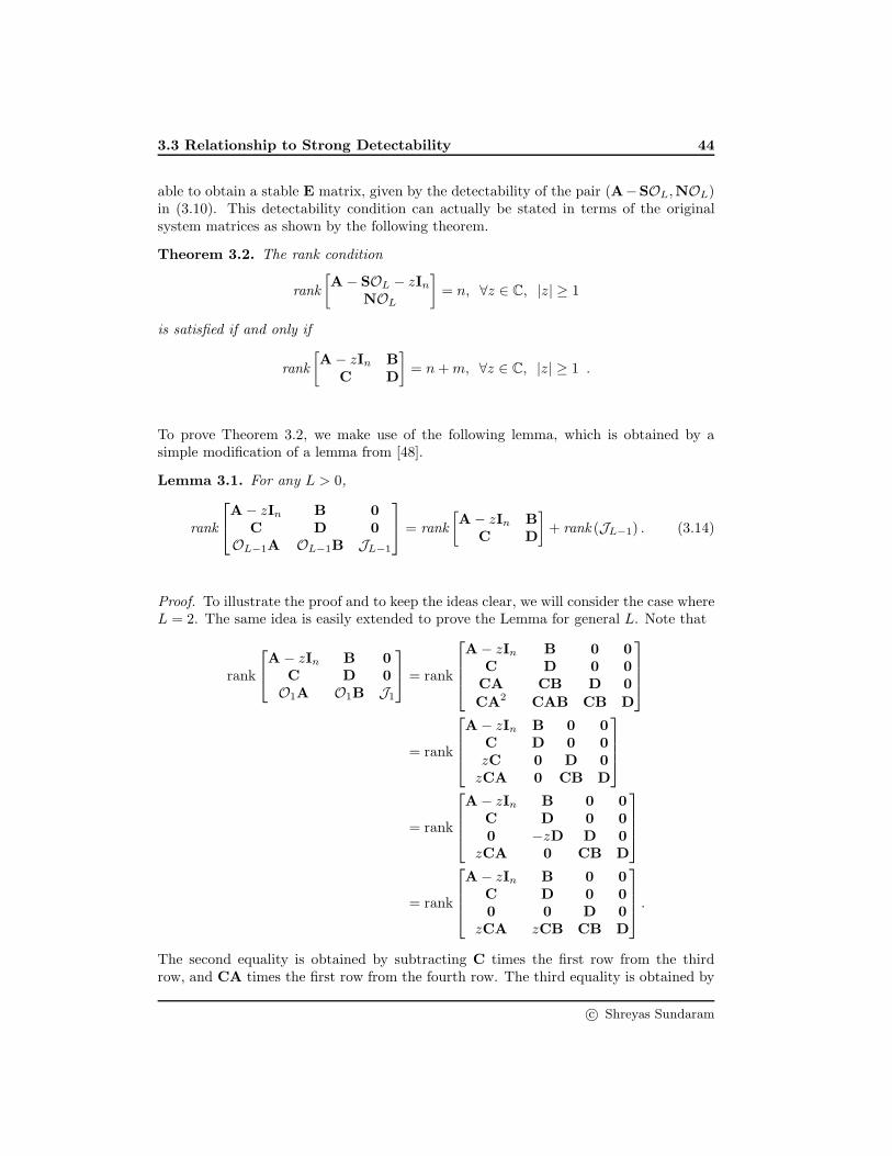
3.3 Relationship to Strong Detectability 44
able to obtain a stable E matrix, given by the detectability of the pair (A−SOL,NOL)in (3.10). This detectability condition can actually be stated in terms of the originalsystem matrices as shown by the following theorem.
Theorem 3.2. The rank condition
rank
[A− SOL − zIn
NOL
]
= n, ∀z ∈ C, |z| ≥ 1
is satisfied if and only if
rank
[A− zIn B
C D
]
= n+m, ∀z ∈ C, |z| ≥ 1 .
To prove Theorem 3.2, we make use of the following lemma, which is obtained by asimple modification of a lemma from [48].
Lemma 3.1. For any L > 0,
rank
A− zIn B 0C D 0
OL−1A OL−1B JL−1
= rank
[A− zIn B
C D
]
+ rank (JL−1) . (3.14)
Proof. To illustrate the proof and to keep the ideas clear, we will consider the case whereL = 2. The same idea is easily extended to prove the Lemma for general L. Note that
rank
A− zIn B 0C D 0
O1A O1B J1
= rank
A− zIn B 0 0C D 0 0CA CB D 0
CA2 CAB CB D
= rank
A− zIn B 0 0C D 0 0zC 0 D 0zCA 0 CB D
= rank
A− zIn B 0 0C D 0 00 −zD D 0
zCA 0 CB D
= rank
A− zIn B 0 0C D 0 00 0 D 0
zCA zCB CB D
.
The second equality is obtained by subtracting C times the first row from the thirdrow, and CA times the first row from the fourth row. The third equality is obtained by
c© Shreyas Sundaram

3.3 Relationship to Strong Detectability 45
subtracting z times the second row from the third row. The fourth equality is obtainedby adding z times the third column to the second column. Repeating this sequence, weobtain
rank
A− zIn B 0 0C D 0 00 0 D 0
zCA zCB CB D
= rank
A− zIn B 0 0C D 0 00 0 D 0
z2C 0 CB D
= rank
A− zIn B 0 0C D 0 00 0 D 00 −z2D CB D
= rank
A− zIn B 0 0C D 0 00 0 D 00 0 CB D
= rank
[A− zIn B
C D
]
+ rankJ1.
This concludes the proof.
We are now in place to prove Theorem 3.2.
Proof. From the definition of S and N, we note that both of these matrices are in the
left nullspace of the matrix
[0
JL−1
]
(i.e., the last Lm columns of JL). Let N be a matrix
whose rows form a basis for the left nullspace of JL−1. We can then write
S = Q1
[Ip 00 N
]
, N = Q2
[Ip 00 N
]
for some matrices Q1 and Q2. Consider the matrix
[D
NOL−1B
]
. As the system is
invertible with delay L, this matrix has rank m. Let Q3 be any left inverse of thismatrix. Since NJL = 0, we have that
Q2
[Ip 00 0
] [D
OL−1B
]
= 0,
and thus the rows of Q2 form a basis for the left nullspace of
[D
NOL−1B
]
. Thus the
matrix
[Q2
Q3
]
is square and invertible. Furthermore, since
S
[D
OL−1B
]
= Q1
[D
NOL−1B
]
= B,
c© Shreyas Sundaram
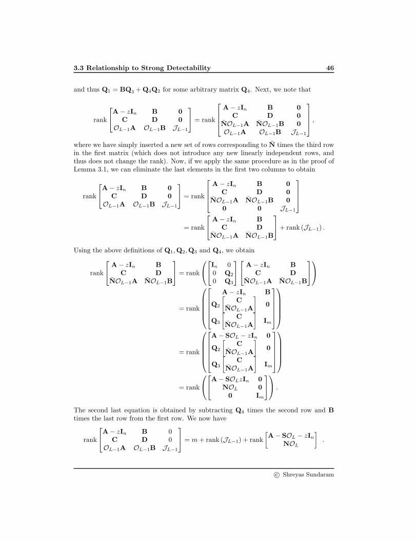
3.3 Relationship to Strong Detectability 46
and thus Q1 = BQ3 +Q4Q2 for some arbitrary matrix Q4. Next, we note that
rank
A− zIn B 0C D 0
OL−1A OL−1B JL−1
= rank
A− zIn B 0C D 0
NOL−1A NOL−1B 0OL−1A OL−1B JL−1
,
where we have simply inserted a new set of rows corresponding to N times the third rowin the first matrix (which does not introduce any new linearly independent rows, andthus does not change the rank). Now, if we apply the same procedure as in the proof ofLemma 3.1, we can eliminate the last elements in the first two columns to obtain
rank
A− zIn B 0C D 0
OL−1A OL−1B JL−1
= rank
A− zIn B 0C D 0
NOL−1A NOL−1B 00 0 JL−1
= rank
A− zIn BC D
NOL−1A NOL−1B
+ rank (JL−1) .
Using the above definitions of Q1,Q2,Q3 and Q4, we obtain
rank
A− zIn BC D
NOL−1A NOL−1B
= rank
In 00 Q2
0 Q3
A− zIn BC D
NOL−1A NOL−1B
= rank
A− zIn B
Q2
[C
NOL−1A
]
0
Q3
[C
NOL−1A
]
Im
= rank
A− SOL − zIn 0
Q2
[C
NOL−1A
]
0
Q3
[C
NOL−1A
]
Im
= rank
A− SOLzIn 0NOL 00 Im
.
The second last equation is obtained by subtracting Q4 times the second row and Btimes the last row from the first row. We now have
rank
A− zIn B 0C D 0
OL−1A OL−1B JL−1
= m+ rank (JL−1) + rank
[A− SOL − zIn
NOL
]
.
c© Shreyas Sundaram

3.3 Relationship to Strong Detectability 47
Using Lemma 3.1, we get
rank
[A− zIn B
C D
]
= m+ rank
[A− SOL − zIn
NOL
]
,
and thus the matrix on the left has rank n +m for all z ∈ C, |z| ≥ 1 if and only if thematrix on the right has rank n for all such z.
From Theorem 3.1, Theorem 3.2, and our discussion so far, we immediately obtain thefollowing theorem.
Theorem 3.3. The system (3.1) has an observer with delay L if and only if
1. rank (JL)− rank (JL−1) = m,
2. rank
[A− zI B
C D
]
= n+m, ∀z ∈ C, |z| ≥ 1.
Recall that the first condition in the above theorem means that the system is invertiblewith delay L + 1. However, the second condition was shown in Theorem 2.7 of Sec-tion 2.9.2 (and [60]) to be sufficient for the existence of an inverse. This leads to thefollowing theorem.
Theorem 3.4. The system S in (3.1) has an observer (possibly with delay) if and onlyif
rank
[A− zI B
C D
]
= n+m, ∀z ∈ C, |z| ≥ 1 .
From Section 2.9.3, we see that this is the condition for the system to be strongly de-tectable, and thus strong detectability and the ability to construct an unknown inputobserver are equivalent.
c© Shreyas Sundaram

Chapter 4
Fault-Detection and Isolation
Schemes
In the last chapter, we saw how to design observers for systems with unknown inputs; ifthe system is strongly detectable, then one can recover the state of the system and theunknown inputs (e.g., faults) via such an observer. However, if there are a large numberof potential faults in the system, treating them all as unknown inputs may cause thesystem to no longer be strongly detectable. In such cases, if we assume that only a smallnumber of all potential faults can occur at any given time, one can tailor observer-basedschemes to detect and identify such faults. We will examine these schemes here. Thematerial in this section follows Chapters 1-3 of [63], the survey paper [21], and the paper[12].
4.1 Sensor Fault Detection
Consider the system
x[k + 1] = Ax[k] +Bu[k],
where u is a known input. Suppose that the system has p outputs, given by the vector
y[k] =
y1[k]y2[k]...
yp[k]
.
If sensor i is faulty at a given time-step k, the output provided by it can be modeled asyi[k] = Cix[k] + fi[k], where Ci is a row vector and fi[k] is an additive error. Thus theoverall output of the system is given by
y[k] = Cx[k] + f [k],
c© Shreyas Sundaram

4.1 Sensor Fault Detection 49
where f [k] is the vector of all additive errors at time-step k. Our objective in thissection will be to detect and identify any single sensor fault (i.e., determine which, ifany, component of f [k] is nonzero). The architecture that we will be using to achievethis is shown below:
The main tool to perform diagnosis will be a state-estimator (studied in Section 2.8).Specifically, consider the output of any given sensor yi[k] = Cix[k]+fi[k], and constructa state-estimator of the form
x[k + 1] = Ax[k] +Bu[k] + L(yi[k]−Cix[k])
= (A− LCi)x[k] +Bu[k] + Lyi[k].
As before, define the estimation error e[k] = x[k]− x[k], and examine
e[k + 1] = x[k + 1]− x[k + 1] = (A− LCi)e[k]− Lfi[k].
Note that the estimation error is now affected by the sensor fault fi[k]. Recall that ifthe pair (A,Ci) is observable, then one can choose L so that the matrix A − LCi hasall eigenvalues at any desired locations. Specifically, one could choose all eigenvalues tobe at zero, which would cause e[k] → 0 in n time-steps if fi[k] is zero over that time(i.e., the i–th sensor is perfectly reliable over the first n time-steps). Given the estimatedstate x[k], define the estimated output y[k] = Cx[k], and note that y[k] − y[k] → 0 iffi[k] is zero. The j–th component of y[k], denoted by yj [k] = Cj x[k] gives the estimatedoutput of the j–th sensor.
Define the p− 1 residual signals
rj [k] = yj [k]− yj [k], j = 1, 2, . . . , p, j 6= i.
As noted above, if sensor i is perfect then yj [k] → Cjx[k]. However, if sensor j has afault, then yj [k] = Cjx[k] + fj[k], and thus rj [k] = Cjx[k] + fj [k]−Cj x[k] → fj [k]. Onthe other hand, if sensor i itself is faulty, then many (and perhaps all) of the estimatedoutputs will not match the actual outputs provided by the other (correct) sensors. Thedetection logic is therefore as follows:
c© Shreyas Sundaram

4.2 Robust Fault Detection and Identification 50
Suppose that at most one sensor can be faulty at any time-step k.If rj [k] 6= 0 for only one j ∈ {1, 2, . . . , i−1, i+1, . . . , p}, then sensorj is faulty. If rj [k] 6= 0 for all j ∈ {1, 2, . . . , i− 1, i+ 1, . . . , p}, thensensor i is faulty.
Example 4.1. Consider the system
A =1
2
1 1 0 10 1 1 01 0 1 10 0 1 1
, C =
1 0 0 00 1 0 00 1 1 0
.
We will assume for simplicity that the known inputs are zero (if not they can be handledas in Section 2.8). Consider sensor 1, which provides the output y1[k] = C1x[k] =[1 0 0 0
]x[k] under fault-free circumstances. One can verify that the pair (A,C1)
is observable, and thus we can use just this output to construct a state estimator of theform
x[k + 1] = Ax[k] + L(yi[k]−Cix[k]) = (A− LCi)x[k] + Lyi[k].
The estimation error is given by e[k + 1] = (A− LCi)e[k] (when the fault is zero), andwe choose the matrix L so that all eigenvalues of A − LCi are at zero; this is achievedvia
L =
21.52.52
.
With this matrix, we find that (A− LCi)4 = 0, and thus e[4] = (A − LCi)
4e[0] = 0 ifthere are no faults during the first 5 time-steps.
Now construct the output estimates y2[k] = C2x[k] and y3[k] = C3x[k], and the residuals
r2[k] = y2[k]− y2[k], r3[k] = y3[k]− y3[k].
If there are no faults in the first five time-steps, we have r2[k] = 0 and r3[k] = 0 afterk = 5. However, now suppose that there is a fault in sensor 2 starting at time-step 20,with additive error f2[k] = 2. The residual r2[k] then becomes equal to 2 after time-step20, while r3[k] stays zero. Thus, we can determine that sensor 2 is faulty.
4.2 Robust Fault Detection and Identification
We will now consider systems that are affected by faults, together with disturbances.Such systems can be modeled as follows:
x[k + 1] = Ax[k] +Bdd[k] +Bf f [k]
y[k] = Cx[k] +Ddd[k] +Df f [k].(4.1)
c© Shreyas Sundaram

4.2 Robust Fault Detection and Identification 51
where d ∈ Rmd is the disturbance, and f ∈ Rmf is the fault. We have omitted knowninputs in the above equation, but they can easily be handled. The values of d[k] andf [k] are unknown at each time-step; however, d[k] is assumed to be active at all time,whereas f [k] is assumed to be intermittently nonzero (corresponding to transient faults),nonzero only after some time, or sparse (corresponding to only a few of the faults beingactive). Note that the above model is able to capture actuator faults, plant faults, andsensor faults. The output of the system over L+ 1 time-steps is given by
y[k : k + L] = OLx[k] + J dLd[k : k + L] + J f
L f [k : k + L], (4.2)
where J dL and J f
L are the invertibility matrices for the systems (A,Bd,C,Dd) and(A,Bf ,C,Df ), respectively. As described in the last section, if the system
(A,[Bd Bf
],C,
[Dd Df
])
is strongly detectable, one can construct an unknown input observer for the system andrecover both f [k] and d[k], regardless of their values. However, when there are a largenumber of possible faults, decoupling them all simultaneously will often not be possible.In such cases, one can operate under the assumption that only one (or a few) of thefaults will be active. Since the disturbances are assumed to be present all the time (e.g.,wind on an airplane), our objective will be to construct an observer to decouple only thedisturbances, and then use the estimation error to infer the presence of any faults.
4.2.1 Fault Detection: Single Observer Scheme
Here, we design an unknown input observer to only decouple the disturbances, assumingthat the faults are zero. When we run the resulting state-estimator, and the fault isnonzero, that will hopefully show up as a difference in the estimated outputs and theactual outputs, from which we can detect the presence of the fault.
To this end, consider the estimator
x[k + 1] = Ex[k] + Fy[k : k + L]
where E and F are chosen so that e[k] = x[k] − x[k] → 0, regardless of d[k], and whenf [k] = 0 for all k. This can be done as long as (A,Bd,C,Dd) is strongly detectable.More specifically,
e[k + 1] ≡ x[k + 1]− x[k + 1]
= Ex[k] + Fy[k : k + L]−Ax[k]−Bdd[k]−Bf f [k]
= Ee[k] + Fy[k : k + L] + (E−A)x[k]−Bdd[k]−Bf f [k] .
Using (4.2), the error can then be expressed as
e[k + 1] = Ee[k] + Fy[k : k + L] + (E−A)x[k]−Bdd[k]−Bf f [k]
= Ee[k] + (E−A+ FOL)x[k] + FJ dLd[k : k + L]−Bdd[k]
+ FJ fL f [k : k + L]−Bf f [k] .
c© Shreyas Sundaram

4.2 Robust Fault Detection and Identification 52
As in the last chapter, if the system (A,Bd,C,Dd) is strongly detectable, we can chooseE and F so that FJ d
L =[Bd 0 · · · 0
]and E = A− FOL is stable. This produces
e[k + 1] = (A− FOL)e[k] + FJ fL f [k : k + L]−Bf f [k], (4.3)
from which e[k] → 0 if f [k] = 0 for all k. We will now define a residual function
r[k] = H1x[k] +H2y[k : k + L]
that is supposed to satisfy the property that r[k] = 0 if f [k] = 0, and r[k] 6= 0 otherwise.Expanding the above expression, we obtain
r[k] = H1e[k] +H1x[k] +H2OLx[k] +H2J dLd[k : k + L] +H2J f
L f [k : k : L].
When f [k] = 0, we can choose H1 = −H2OL, and H2 to be a matrix whose rows forma basis for the left nullspace of J d
L , yielding
r[k] = H1e[k] +H2J fL f [k : k : L]. (4.4)
Equations (4.3) and (4.4) together form the residual generator, and if f [k] = 0, we havee[k] → 0 and r[k] → 0. However, if f [k] becomes nonzero after some time, then we wouldexpect e[k] and r[k] to be nonzero, from which we can detect the presence of the fault.
Remark 4.1. Note that this method does not guarantee that all possible faults willbe detected. Since the system is assumed to not be strongly detectable (otherwise wecould design a UIO for the entire system, including faults), there is an input and a setof faults and disturbances such that the output is zero for all time. Clearly such faultsand disturbances cannot be detected; the above method assumes that the faults to thesystem are not applied in this “worst case” manner, so that the output of the systemdoes in fact indicate the presence of a fault (via the state-estimator and the residual).
Example 4.2. Consider the system
x[k + 1] =1
2
1 1 0 10 1 1 01 0 1 10 0 1 1
︸ ︷︷ ︸
A
x[k] +
1 00 10 11 1
︸ ︷︷ ︸
Bf
f [k] +
0101
︸︷︷︸
Bd
d[k]
y[k] =
1 0 0 00 1 0 00 1 1 0
x[k].
Using the design procedure in Chapter 3, we construct an unknown input observer forthe system (A,Bd,C,0), producing
x[k + 1] =
0 0.3077 −0.1538 0.6923 −0.3077 0.30770 0.1538 −0.0769 −0.1538 0.8462 0.15380 −0.3077 0.1538 0.3077 −0.6923 0.6923
−0.5 −0.2308 −0.3846 0.2308 0.2308 0.7692
︸ ︷︷ ︸
F
y[k : k + 1].
c© Shreyas Sundaram

4.2 Robust Fault Detection and Identification 53
Note that the E matrix is zero in this case (we placed all of the eigenvalues at 0). Next,to design the residual (4.4), we choose the matrix H2 to form a basis for the left nullspaceof
J d1 =
[Dd 0CBd Dd
]
=
0 00 00 00 01 01 0
,
which gives
H2 =
1 0 0 0 0 00 1 0 0 0 00 0 1 0 0 00 0 0 1 0 00 0 0 0 −1 1
.
Finally, we have
H1 = −H2O1 =
−1 0 0 00 −1 0 00 −1 −1 0
−0.5 −0.5 0 −0.5−0.5 0 −0.5 −0.5
.
If there are no faults in the system, the residual r[k] = H1x[k] +H2y[k : k+ 1] is foundto be zero. However, if one or both of the faults become active (say, equal to 2 over someperiod of time), we find that the residual also becomes nonzero over that time-period,and thus we are able to detect the fault.
4.2.2 Single Fault Identification: Bank of Observers
The method described in the previous section used a single observer to decouple thedisturbances, and a nonzero residual was used to infer the presence of a fault. However,the above scheme generally does not allow us to identify which of the possible faultscaused the nonzero residual (i.e., which entry of f [k] is nonzero). To identify faults, wewill use a scheme similar to that described at the beginning of the chapter for sensorfaults. Specifically, we will design a bank of observers, each of which will provide aresidual that will allow us to identify a single fault at a time.
First, recall from Section 2.9.3 that a system is strongly detectable only if the number ofunknown inputs is less than the number of outputs. Let mf be the number of possiblefaults, and let md be the number of disturbances. Now we will design mf differentobservers as follows. For observer i, we group fault i with the disturbances, and treatit as an unknown input. Specifically, let Bi
f denote the i–th column of Bf , and let B−if
denote all other columns. Similarly, let fi[k] denote the i–th component of f [k] and let
c© Shreyas Sundaram

4.2 Robust Fault Detection and Identification 54
f−i[k] denote all other components. Rearranging (4.1), we can write
x[k + 1] = Ax[k] +B−if f−i[k] +
[Bd Bi
f
][d[k]fi[k]
]
y[k] = Cx[k] +D−if f−i[k] +
[Dd Di
f
][d[k]fi[k]
]
.
If the system (A,[Bd Bi
f
],C,
[Dd Di
f
]) is strongly detectable, we can create an
unknown input observer for this system, treating the vector
[d[k]fi[k]
]
as the unknown
inputs. Furthermore, we can design a residual ri[k] for this system; let the residualgenerator be given by
xi[k + 1] = Eixi[k] + Fiy[k : k + L]
ri[k] = Hi1xi[k] +Hi2y[k : k + L].
As in the last section, if Hi1 and Hi2 are chosen appropriately, we will have ri[k] =0 if f−i[k] = 0, and ri[k] 6= 0 otherwise. Thus, we can determine which faults areactive simply by examining which of the residuals are nonzero. Specifically, residualri[k] depends on all faults except fi[k]. The detection logic is as follows.
If all residuals except ri[k] are nonzero, and ri[k] is zero, then faulti has occurred.
Note that only one fault can be identified via the above scheme.
4.2.3 Multiple Fault Identification: Dedicated Observers
If we would like to be able to simultaneously identify multiple faults, we can extendthe scheme in the previous section as follows. As in the last section, we will design mf
different observers. For observer i, we group all faults except fault i with the disturbances,and treat them all as unknown inputs. Specifically, let Bi
f denote the i–th column of
Bf , and let B−if denote all other columns. Similarly, let fi[k] denote the i–th component
of f [k] and let f−i[k] denote all other components. Rearranging (4.1), we can write
x[k + 1] = Ax[k] +Biffi[k] +
[Bd B−i
f
][d[k]f−i[k]
]
y[k] = Cx[k] +Diffi[k] +
[Dd D−i
f
][d[k]f−i[k]
]
.
If the system (A,[Bd B−i
f
],C,
[Dd D−i
f
]) is strongly detectable, we can create an
unknown input observer for this system, treating the vector
[d[k]f−i[k]
]
as the unknown
c© Shreyas Sundaram

4.3 Parity Space Methods 55
inputs. Furthermore, we can design a residual ri[k] for this system; let the residualgenerate for the system be given by
xi[k + 1] = Eixi[k] + Fiy[k : k + L]
ri[k] = Hi1xi[k] +Hi2y[k : k + L].
As in the last section, if Hi1 and Hi2 are chosen appropriately, we will have ri[k] = 0if fi[k] = 0, and ri[k] 6= 0 otherwise. Thus, we can determine which faults are activesimply by examining which of the residuals are nonzero.
If residual ri[k] is nonzero, then fault i has occurred.
It is instructive to compare the scheme in this section to the previous one. Note thatin order to identify multiple faults, we had to group all but one of the faults into theunknown inputs, together with the disturbances. This could potentially add a largenumber of unknown inputs to the system, preventing it from being strongly detectable.In contrast, the scheme in the previous section only adds a single fault to the unknowninputs for each observer. Thus, the former scheme can be applied to a larger class ofsystems than the scheme described in this section.
4.3 Parity Space Methods
In the last two sections, we used observer-based methods to generate residuals for faultdetection and identification. One can also try to diagnose faults directly from the outputsof the system, without constructing an observer (this would be useful, for example, ifthe system is not strongly detectable). This is called the parity space method.
First, note that the output of the system (4.1) over any L + 1 time-steps is given by(4.2). In this equation, the quantities x[k], f [k : k + L] and d[k : k + L] are all unknown(assuming that an unknown input observer for x[k] has not been constructed). However,for the purposes of fault diagnosis, we are only interested in recovering information aboutf [k : k + L], so we would like to eliminate the effect of the other unknown quantities onthe output. To do this, define the matrix V such that the rows form a basis for the leftnullspace of
[OL J d
L
].
Definition 4.1. The space spanned by the rows of V is called theparity space of the system.
c© Shreyas Sundaram

4.3 Parity Space Methods 56
If we multiply the output of the system by V, we obtain
Vy[k : k + L]︸ ︷︷ ︸
r[k]
= VOLx[k] +VJ fL
︸ ︷︷ ︸
P
f [k : k + L] +VJ dLd[k : k + L]
= Pf [k : k + L].
The quantity r[k] is the residual, and is used to diagnose the presence of faults. Inthis context, the residual is also known as a syndrome in the coding-theory literature,which we will study later. The residual lies in the range-space of the matrix P, andcharacterizes the (isolated) effects of the faults on the output over L + 1 time-steps. Ifcolumn i of P is nonzero, then if the i-th element of f [k : k+L] is nonzero and everythingelse is zero, the residual will be nonzero, which means that the fault will be detected.
Similarly, if column i is linearly independent of any other single column, then one canidentify that the i–th element of f [k : k + L] is nonzero, as long as only one elementof f [k : k + L] is nonzero. To see this, let pi denote the i–th column of P, and let fidenote the value of the i–th element of f [k : k + L]. If fi is the only nonzero element off [k : k+L], the residual is given by r[k] = pifi. This means that the residual is a scaledversion of pi. The only way we could not identify that fi is the nonzero element is ifthere is some other nonzero element of f [k : k +L], say fj , that could produce the sameresidual. This would mean that
r[k] = pifi = pjfj ⇒ pifi − pjfj = 0.
This means that column pi and pj would have be linearly dependent, which is not thecase by assumption.
More generally, if a given set of t columns of P are linearly independent of any other setof t columns, then we could uniquely identify the faults corresponding to those t columns(this can be shown by following an identical argument to the case where t = 1 consideredabove).
Example 4.3. Consider the system
x[k + 1] =
1 1 0 10 1 1 01 0 1 10 0 1 1
︸ ︷︷ ︸
A
x[k] +
1 00 10 11 1
︸ ︷︷ ︸
Bf
f [k] +
0101
︸︷︷︸
Bd
d[k]
y[k] =
1 0 0 00 1 0 00 1 1 0
x[k].
Consider the output of the system over 4 time-steps (i.e., L = 3). A basis V for the left
c© Shreyas Sundaram

4.3 Parity Space Methods 57
nullspace of[O3 J d
3
]is found, and is used to calculate
P = VJ fL =
−1 1 0 0 0 0 0 00 0 1 0 0 0 0 0
−1 1 0 1 0 0 0 00 0 2 0 1 0 0 0
−1 1 2 1 0 1 0 0
.
Note that the last two columns of P are zero, so we will not be able to detect or identifyany faults in the last two elements of f [k : k + 3], or equivalently, in f [3]. However, allother columns are nonzero, so if any single element of f [k : k+2] (i.e., all but the bottomtwo elements) is nonzero, this will be detected.
Next, note that the first column is just the negative of the second column. Thus, if f [k]
is of the form
[aa
]
for any a, we would not be able to detect this behavior. Thus we are
not guaranteed to be able to detect any two faults in f [k : k + 3] (in the worst case).However, note that columns 3, 4, 5 and 6 are linearly independent of all other columns.Thus, any nonzero entries in the third, fourth, fifth and sixth elements of f [k : k+3] areguaranteed to be identified (these elements correspond to f [k + 1] and f [k + 2]).
For example, suppose that the residual is given by
r[k] =
03066
.
This is a multiple of the third column, and thus we know that the third element off [k : k + 3] is nonzero, with value 3.
For this example, if we assume that there is at most one fault in any L + 1 time-steps,we can uniquely identify the fault if it occurs in f [k + 1] or f [k + 2].
c© Shreyas Sundaram

Chapter 5
Reliable System Design
In the previous sections, we have been concerned with detecting and identifying faultsthat occur in a given system. We now turn our attention to constructing reliable systems.We will consider various fault models, and describe schemes that can be used to handleeach of those models. We will start our investigation by considering an intuitive majorityvoting scheme.
5.1 Majority Voting with Unreliable Components
As described in Chapter 1, majority voting is perhaps the most direct method of im-plementing fault-tolerance. Specifically, suppose that we have a certain component thatcould malfunction. In order to obtain reliable behavior, one could simply replicate thiscomponent, and then use some logic to compare the outputs to decide which one to use.For example, consider designing a controller for a given system. In Section 2.8, we sawthat we could design a state-estimator for the system, and then use observer feedbackto control the system. The architecture is as follows:
The controller in this case is given by the state-estimator together with the feedbackinput. Now, if the controller experiences a fault, one could potentially apply an incorrect(or destabilizing) input to the system. To prevent this, we can replicate the controllerthree times, and then simply use a majority voter to apply the input that is specified by
c© Shreyas Sundaram

5.1 Majority Voting with Unreliable Components 59
the majority of the controllers; this is guaranteed to work if at most one of the controllersis assumed to be faulty at any given time-step. More generally, if we want to tolerate upto f faulty controllers at any given time-step, we should use a bank of 2f +1 redundantcontrollers, and apply the value specified by at least f + 1 of them.
The above procedure works if one considers that a bounded number of faults occur, andthat the majority voter itself is reliable. However, what happens if the components arefaulty with a certain probability, and the voter itself can choose an incorrect value witha certain probability? This problem was studied in the seminal paper [92] by John VonNeumann, and we will discuss the main ideas here.
The paper considers the case where each component outputs a binary value 0 or 1.However, the component can be faulty with probability η, in which case it outputs a 0when it should have output a 1, and vice versa. Note that there is a possibility that twoor more of the components can be faulty, under this model. Specifically, the probabilitythat at least two components are faulty is given by
θ =
(3
2
)
η2(1− η) + η3 = 3η2 − 2η3. (5.1)
If the majority voter is operating correctly, it should output a 1 if at least two of itsinputs are 1, and 0 otherwise. However, the voter itself can be faulty with probabilityǫ, whereby it outputs a 1 when the majority of its inputs are 0, and vice versa. Wewill assume throughout that η ≤ 1/2 and ǫ ≤ 1/2, because otherwise, the correspondingcomponent is “wrong more often than right”, and thus we can simply flip the valuethat it provides us to obtain a value that is incorrect with probability 1 − η < 1/2 and1− ǫ < 1/2.
The output of the entire mechanism (the three redundant components and the majorityvoter together) can be incorrect with a certain probability, given by
η∗ = ǫ(1− θ) + (1 − ǫ)θ
= ǫ+ θ(1 − 2ǫ).
Since ǫ < 1/2, we see that 1− 2ǫ > 0, and thus η∗ > ǫ; this is intuitive, since one cannotexpect to obtain a measure of reliability greater than the reliability of the last componentin the chain. The above expression shows that the probability of a faulty output exceedsthe minimum possible probability ǫ by the quantity θ(1 − 2ǫ). To investigate η∗ morecarefully, use (5.1) in the above expression to obtain
η∗ = ǫ+ (3η2 − 2η3)(1− 2ǫ).
c© Shreyas Sundaram

5.1 Majority Voting with Unreliable Components 60
Note that if ǫ = 12 , we have η
∗ = ǫ = 12 , regardless of η. This is intuitive: if the majority
voter is completely arbitrary (i.e., it is correct or incorrect with equal probability), theoutput of the majority voter can never be trusted, regardless of how reliable the individualcomponents themselves are. A plot of η∗ versus η for various nonzero values of ǫ is shownin Figure 5.1.
0 0.1 0.2 0.3 0.4 0.5 0.6 0.7 0.8 0.9 10
0.1
0.2
0.3
0.4
0.5
0.6
0.7
0.8
0.9
1
η
η∗
η∗ = ηε = 0.05ε = 1/6ε = 0.4
Figure 5.1: Variation of η∗ versus η for various values of ǫ.
The straight diagonal line in the figure represents the case where η∗ = η (i.e., theprobability of error at the output of the majority-voting system is equal to the probabilityof error of any of the individual components). Clearly, we would like to do better thanthis, because otherwise we are gaining nothing from the majority voting system. Next,note that for small values of ǫ, this is in fact possible. For example, when ǫ = 0.05 and0.059 < η < 0.5, we have η∗ < η. For η < 0.059, however, we have η∗ > η; this isbecause the unreliable majority voter becomes the bottleneck in this case. The mainpoint is that for small ǫ, the majority voter scheme does, in fact, reduce the probabilityof error at the output, compared to any single component on its own.
Now consider the case where ǫ = 16 in Figure 5.1. Here, the curve η∗ is always above η
for 0 ≤ η < 0.5, and crosses only at η = 0.5. Thus, for ǫ = 16 , the majority voter does
not do better than the single component acting on its own. The same is true for ǫ > 16 ,
as shown in the figure.
Based on the above analysis, we see that we will get an improvement via the majorityvoting scheme if and only if the curve η∗ = ǫ + (3η2 − 2η3)(1 − 2ǫ) crosses the curveη∗ = η more than once. To find the set of ǫ’s for which this happens, we set the two
c© Shreyas Sundaram

5.1 Majority Voting with Unreliable Components 61
expressions equal to each other to find the points of intersection:
ǫ+ (3η2 − 2η3)(1− 2ǫ) = η ⇔ 2(1− 2ǫ)η3 − 3(1− 2ǫ)η2 + η − ǫ︸ ︷︷ ︸
f(η)
= 0.
As indicated by the figures above, η = 12 is always a root of f(η). Factoring out η − 1
2 ,we obtain
f(η) = 2
(
η − 1
2
)
((1 − 2ǫ)η2 − (1− 2ǫ)η + ǫ).
Thus, the other intersections are given by the roots of (1 − 2ǫ)η2 − (1 − 2ǫ)η + ǫ; usingthe quadratic formula, we obtain
η =(1 − 2ǫ)±
√
(1− 2ǫ)2 − 4(1− 2ǫ)ǫ
2(1− 2ǫ)=
1
2± 1
2
√
1− 6ǫ
1− 2ǫ.
Since 1 − 2ǫ > 0 (by assumption), we see that f(η) will have three (real) roots if andonly if 1− 6ǫ > 0, or equivalently, ǫ < 1
6 . Thus, we have analytically verified the boundthat we observed in the figure. Thus, we obtain the following result.
Suppose that each component is faulty with a probability η, andthat the majority voter is faulty with probability ǫ (with both 0 ≤η ≤ 1
2 and 0 ≤ ǫ ≤ 12 ). Then the output of a majority voting system
with three redundant components is faulty with probability
η∗ = ǫ+ (3η2 − 2η3)(1− 2ǫ).
Furthermore, it is possible to have η∗ < η only if ǫ < 16 .
The above result shows that we can reduce the probability of a fault via a majorityvoting scheme (only ǫ < 1
6 ); furthermore, we argued earlier that the probability of afault can never fall below ǫ (the probability that the majority voter itself is faulty). Wecan now ask the question: how close can we bring the fault probability to ǫ? To answerthis question, suppose that ǫ < 1
6 , and consider the following architecture:
c© Shreyas Sundaram

5.2 A Coding-Theory Approach to Reliable Controller Design 62
The output of each of the first line of majority voters is incorrect with probability η∗ < η.We can now repeat the above analysis to see that the output of the last majority voter isfaulty with probability η∗∗ < η∗ < η. Essentially, every time we repeat this process, we‘slide’ down the curve ǫ+(3η2−2η3)(1−2ǫ) to the point where ǫ+(3η2−2η3)(1−2ǫ) = η,given by
1
2− 1
2
√
1− 6ǫ
1− 2ǫ.
This defines the lower bound on the fault probability, using a triple-modular-redundancyarchitecture of the form studied in this section. Note that this lower bound is achievableto an arbitrary degree of precision by creating a long enough chain of majority voters.The price paid for this, of course, is an exponential growth in the number of componentsrequired (3l, where l is the length of the chain), and thus this approach is infeasible inpractice, but the bound (and the technique use to derive it) is useful.
Note that if ǫ > 16 , repeated majority voters will not help; at every time, the probability
of error at the output of each majority voter is worse than the probability of error in anyof the inputs, which drives the error probability closer and closer to 1
2 , meaning that onecould never obtain any useful information from the output of the last majority voter.
5.2 A Coding-Theory Approach to Reliable Controller
Design
In the last section, we considered a majority voting scheme to improve the reliability offaulty components (such as controllers in a feedback loop). This mechanism is simpleto implement, and is able to handle arbitrary failures in the controllers (i.e., it does notmatter why the output is incorrect). However, we saw that this required a great deal ofredundancy. In this section, we will consider a different approach to protecting controllersagainst a certain number of faults that affect their internal state by using coding-theoryto add a small amount of redundancy to the controller itself. This approach was devisedin [30, 32], and the material in this section is from those papers.
5.2.1 Background on Parity-Check Codes
We will start by reviewing some background on coding schemes for reliable informationtransmission. Consider the following simple example. Suppose that we wish to sendthe string of numbers (m1,m2,m3,m4,m5) = (5, 21, 13, 14, 19) across a channel. Forconvenience, we will represent this string by a vector
m =
m1
m2
m3
m4
m5
.
c© Shreyas Sundaram

5.2 A Coding-Theory Approach to Reliable Controller Design 63
Suppose that the channel can introduce faults into the transmission, where it changessome of the numbers. One option to make sure that we receive the message reliably isto send the message three times, i.e., send a vector of the form
m =
mmm
.
Then, as long as the same number is not corrupted in two or more of the subvectors, wecould recover the numbers correctly – this is just a majority voting scheme, as before.
However, now suppose that we consider a model for the channel where it only corruptsone of the numbers in the string. As a first case, suppose that we are only interested indetecting such a corruption. One option is certainly to send the string twice, but this ismuch more redundancy than we need (since we are only interested in detecting a singlecorruption). Instead of sending the entire message twice, let us instead send a singleadditional number with the message. Specifically, suppose that we calculate the sum ofthe numbers in the original message, given by s1 = 5+ 21+ 13 + 14 + 19 = 72 and sendthe message
m =
[ms1
]
=
1 0 0 0 00 1 0 0 00 0 1 0 00 0 0 1 00 0 0 0 11 1 1 1 1
︸ ︷︷ ︸
G
m1
m2
m3
m4
m5
.
Now suppose that one of the numbers is corrupted in transmission; for example, let ussay that 21 is changed to 25. The received message is
mf =
52513141972
= m+
040000
︸︷︷︸
f
.
At the receiver, we know that the last number must be equal to the sum of the othernumbers. However, the sum of the first five numbers in the received message is now 76,and this does not match with the last number; thus, we can detect than an error hasoccurred. More formally, we know that for any correct message m, it must be the casethat
r =[1 1 1 1 1 −1
]
︸ ︷︷ ︸
P
m = 0.
Note that the vector P is a basis for the left nullspace of G. For the erroneous message,we have
r = Pmf = P(m + f) = Pf .
c© Shreyas Sundaram

5.2 A Coding-Theory Approach to Reliable Controller Design 64
Suppose a single element of f , say fi is nonzero; this produces r = fi if 1 ≤ i ≤ 5 ands = −fi if i = 6. Thus, r will be nonzero if there is a single fault. However, we cannotdetermine which of the numbers were corrupted, since any of them could have had anerror with value fi added to it. In the language of fault diagnosis from Chapter 4, thenumber r is the residual for this message. As mentioned in the last chapter, the quantityr is also called the syndrome in coding theory [5].
To identify an error, we would have to add more redundancy to the message. Specifically,suppose that we add another number to the message that is generated by taking somelinear combination of the numbers, i.e., s2 = α1m1+α2m2+α3m3+α4m4+α5m5. Thesent message is then
m =
ms1s2
=
1 0 0 0 00 1 0 0 00 0 1 0 00 0 0 1 00 0 0 0 11 1 1 1 1α1 α2 α3 α4 α5
︸ ︷︷ ︸
G
m1
m2
m3
m4
m5
and again, the received message is
mf = m + f ,
where f is an additive error that affects one of the numbers in the message. Once again,let P be a matrix whose rows form a basis for the left nullspace of G; one such matrix is
P =
[1 1 1 1 1 −1 0
α1 α2 α3 α4 α5 0 −1
]
.
Thus, the residual (or syndrome) is given by
r = Pmf = PGm+Pf = Pf .
As in the parity-space fault diagnosis method studied in Section 4.3, the columns of Pdetermine whether we can identify a nonzero element of f . Specifically, we can uniquelyidentify which element is nonzero if the residual can only be generated by a single columnof P. This is accomplished if any two columns of P are linearly independent. To seewhy, suppose that this condition holds, but that two different elements of f , say fi andfj , can produce the same residual, i.e.,
r = pifi = pjfj
where pi and pj are the i–th and j–th columns of P, respectively. However, this wouldimply that pi and pj are linearly dependent, which contradicts the assumption.
So, if α1, α2, . . . , α5 are chosen so that any two columns of P are linearly independent,we can uniquely identify any single fault that affects the message. For example, one canverify that this is achieved by choosing the αi’s to all be different.
c© Shreyas Sundaram

5.2 A Coding-Theory Approach to Reliable Controller Design 65
More generally, suppose that we wish to send k numbers (given by the vector m ∈ Rk,and we generate the transmitted (or redundant) message as follows:
m =
[IkH
]
︸︷︷︸
G
m, (5.2)
where H is a d × k matrix (i.e., we are adding d redundant numbers to the message).The matrix P whose rows form a basis for the left nullspace of G is then given by
P =[H −Id
]. (5.3)
The matrix G is called the generator matrix, and the matrix P is called the parity checkmatrix.
Theorem 5.1. Let t be a nonnegative integer such that any 2tcolumns of P are linearly independent. Then:
• As long as no more than 2t faults occur, they can be detected.
• As long as no more than t faults occur, they call be identified.
Proof. Suppose that 2t or fewer faults occur, so that at most 2t elements of f are nonzero.Thus, the residual is given by
r = Pf
which is a linear combination of at most 2t columns from P. Since any 2t columns arelinearly independent, we see that the residual must be nonzero, and thus these faultscan be detected.
Now suppose instead that t or fewer faults occur, so that at most t elements of f arenonzero. Again, the residual is given by r = Pf , which is now a linear combination of tcolumns of P. We can identify which elements are nonzero if the residual could not havebeen generated by any other set of t nonzero elements. Specifically, suppose that twodifferent sets of t nonzero elements (i.e., two different sets of t faults) can produce thesame residual. Let the fault vectors for these two cases be given by f and f , respectively,where each of those vectors have no more than t nonzero entries. Then if it is the casethat
r = Pf = Pf ,
then, it must be the case that P(f − f) = 0. However, the vector f − f has at most 2tnonzero entries, and thus P(f − f ) is a linear combination of at most 2t columns of P.Since any 2t columns of P are linearly independent, the only way for P(f − f) = 0 is iff − f = 0, i.e., f = f . In other words, as long as there are no more than t faults, everyresidual uniquely determines which set of t faults occurred.
c© Shreyas Sundaram

5.2 A Coding-Theory Approach to Reliable Controller Design 66
Thus, in order to design a message that is resilient to t faults, one must choose the matrixH in (5.2) so that any 2t columns of P in (5.3) are linearly independent. Note that sinceP has d rows, we need d ≥ 2t in order for this to be possible (i.e., we need to add at least2t redundant numbers to the message). Under this condition, there are various ways tochoose H to achieve the desired linear independence. We will see one such scheme in thenext section, when we apply these concepts to designing reliable controllers.
5.2.2 Reliable Controller Design
Suppose that we consider a controller that is a dynamical system of the form
x[k + 1] = Ax[k] +Bu[k]
y[k] = Cx[k],(5.4)
where the state x ∈ Rn. In the previous chapters, we used this notation to representthe plant that we were trying to control, but for convenience, we will use the samenotation here for the controller. Note that the observer-feedback based controllers fromSection 2.8 are of this form. These controllers are simply dynamical systems that areimplemented in a computer: each of the state-variables would be stored in a register,for example. However, digital computers can potentially experience faults; they mightincorrectly perform a computation due to some error, or the contents of certain registersmight get corrupted due to environmental factors, such as alpha particles in aircraft[56, 26]. In this section, we will focus on errors that affect the state-variables in thecontroller, where at some time-step k, some state xi[k] gets changed (erroneously) tosome other state xi[k] + f [k], for some additive error f [k]. Since we are assuming thatwe have access to the entire state of the controller, we will disregard the output ofthe controller y[k] in our investigation, and study how we can add redundancy to thecontroller to detect and identify such state errors.
If we have access to the whole state, why we do not simply just verify that the state isat the correct value by checking whether x[k + 1] = Ax[k] +Bu[k] at each k. However,this essentially amounts to performing the entire state update calculation a second time,which is equivalent to modular redundancy. The goal here is not to replicate the entirecontroller, but to add just enough additional redundancy to detect and identify a fixednumber of state errors. To do this, we will be using the techniques from the previoussection on parity check codes to construct a redundant controller of the form
x[k + 1] = Ax[k] + Bu[k], (5.5)
where the state vector x is of dimension n + d for some nonnegative integer d. Thiscontroller should be designed so that it provides the same functionality as the originalcontroller, but with some additional redundancy. To capture this, the following definitionwas used in [32].
Definition 5.1. The controller (5.5) is a redundant implementation of the controller(5.4) if, for all time-steps k, we have
x[k] = Gx[k], (5.6)
x[k] = Lx[k], (5.7)
c© Shreyas Sundaram
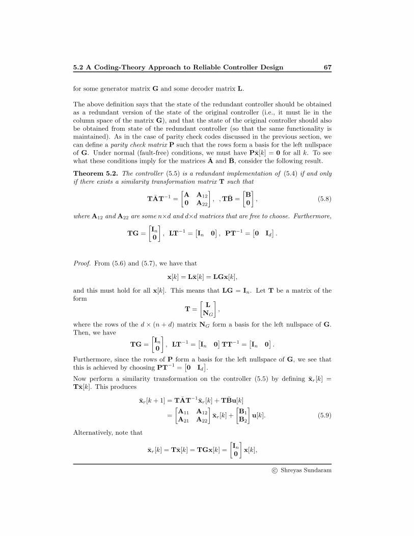
5.2 A Coding-Theory Approach to Reliable Controller Design 67
for some generator matrix G and some decoder matrix L.
The above definition says that the state of the redundant controller should be obtainedas a redundant version of the state of the original controller (i.e., it must lie in thecolumn space of the matrix G), and that the state of the original controller should alsobe obtained from state of the redundant controller (so that the same functionality ismaintained). As in the case of parity check codes discussed in the previous section, wecan define a parity check matrix P such that the rows form a basis for the left nullspaceof G. Under normal (fault-free) conditions, we must have Px[k] = 0 for all k. To seewhat these conditions imply for the matrices A and B, consider the following result.
Theorem 5.2. The controller (5.5) is a redundant implementation of (5.4) if and onlyif there exists a similarity transformation matrix T such that
TAT−1 =
[A A12
0 A22
]
, ,TB =
[B0
]
, (5.8)
where A12 and A22 are some n×d and d×d matrices that are free to choose. Furthermore,
TG =
[In0
]
, LT−1 =[In 0
], PT−1 =
[0 Id
].
Proof. From (5.6) and (5.7), we have that
x[k] = Lx[k] = LGx[k],
and this must hold for all x[k]. This means that LG = In. Let T be a matrix of theform
T =
[LNG
]
,
where the rows of the d × (n + d) matrix NG form a basis for the left nullspace of G.Then, we have
TG =
[In0
]
, LT−1 =[In 0
]TT−1 =
[In 0
].
Furthermore, since the rows of P form a basis for the left nullspace of G, we see thatthis is achieved by choosing PT−1 =
[0 Id
].
Now perform a similarity transformation on the controller (5.5) by defining xr[k] =Tx[k]. This produces
xr[k + 1] = TAT−1xr[k] +TBu[k]
=
[A11 A12
A21 A22
]
xr[k] +
[B1
B2
]
u[k]. (5.9)
Alternatively, note that
xr[k] = Tx[k] = TGx[k] =
[In0
]
x[k],
c© Shreyas Sundaram

5.2 A Coding-Theory Approach to Reliable Controller Design 68
so that
xr[k + 1] =
[x[k + 1]
0
]
=
[Ax[k] +Bu[k]
0
]
.
Substituting this into (5.9), we have
[Ax[k] +Bu[k]
0
]
=
[A11 A12
A21 A22
] [x[k]0
]
+
[B1
B2
]
u[k].
This equation has to hold for all possible values of x[k] and u[k]; in particular, if weconsider u[k] = 0, the bottom row of the above system says that 0 = A12x[k], and thusit must be that A12 = 0. Now, if we allow u[k] to be nonzero, we see that
0 = A220+B2u[k] = B2u[k],
and thus B2 = 0. However, the above equation does not constrain matrices A12 or A22
in any way.
The matrices A12 and A22 are free for us to choose, and characterize all of the freedomthat we have in designing a redundant implementation. Specifically, we will show howto choose these matrices in order to allow detection and identification of a fixed numberof faults.
Detecting and Identifying Faults
Suppose that we have constructed the controller (5.5) so that it is a redundant imple-mentation of the original controller (5.4) (i.e., it satisfies the conditions in Definition 5.1),and that at some time-step k−1, some of the states of the redundant controller becomesaffected by faults as they are being updated. This produces a faulty state
xf [k] = Ax[k] + Bu[k] + f [k]
= x[k] + f [k]
= Gx[k] + f [k],
(5.10)
where fi is a vector with a single nonzero element in its i–th entry, and zeros everywhereelse. Now, let P be a matrix whose rows form a basis for the left nullspace of G (notethat P has dimension d× (n+ d)). We can now calculate the residual (or syndrome)
r[k] = Pxf [k] = PGx[k] +Pf [k] = Pf [k].
Thus, the residual is a linear combination of all columns of P corresponding to theentries of f [k] that are nonzero. As in the previous section, if we want to be able todetect any 2t state-transition faults, or identify any t state-transition faults, we need toany 2t columns of the parity check matrix P to be linearly independent. Rather thanfocusing on designing the system with only this in mind, we will instead consider thefollowing objective. Instead of checking for errors in the state at every time-step, wewould instead like to only check for errors periodically, say, every N time-steps for some
c© Shreyas Sundaram

5.2 A Coding-Theory Approach to Reliable Controller Design 69
N . This would reduce the burden on the checking mechanism, and perhaps allow it tooperate more reliably.
To this end, we will break up the operation of the controller into periods of N time-steps.At the end of each N time-steps, we will examine the state and try to identify any errorsthat occurred during the last period, and then correct all of those errors so the state atthe start of the next period is what it should be. For this reason, we can just considerwhat happens in the firstN time-steps, and the same analysis will hold for all subsequentperiods.
Suppose that the redundant controller is initialized with state x[0] = Gx[0] for someappropriately chosen G (which we will describe later). Any faults that occur at time-step k are captured by the vector f [k], so that the faulty state at time-step k gets updatedaccording to equation (5.10). The faulty state at the end of N time-steps is then givenby
xf [N ] = AN x[0] +[AN−1B AN−2B · · · B
]u[0 : N − 1]
+[AN−1 AN−2 · · · In
]f [0 : N − 1]
= x[N ] +[AN−1 AN−2 · · · In
]f [0 : N − 1]
= Gx[N ] +[AN−1 AN−2 · · · In
]f [0 : N − 1].
If we perform a parity check on this state, we obtain the residual
r[N ] = Pxf [N ] = P[AN−1 AN−2 · · · In
]
︸ ︷︷ ︸
R
f [0 : N − 1]. (5.11)
Thus, the residual is a linear combination of the columns R. Just as before, if we wantto be able to identify up to t errors in a period of N time-steps, we want to make surethat any 2t columns of this matrix are linearly independent. The objective will be tochoose the redundant dynamics A22 and A12 so that this is the case. The followingresult shows how these matrices show up in the matrix R.
Lemma 5.1. If controller (5.5) is a redundant implementation of (5.4), then for anyk, PAk = Ak
22P.
Proof. From Theorem 5.2, we see that there exists a matrix T such that (5.8) holds.
Furthermore, TG =
[In0
]
. Since PG = 0, we see that we can choose PT−1 =[0 Id
].
Thus, we have
PAk = PT−1T
(
T−1
[A A12
0 A22
]
T
)k
=[0 Id
][A A12
0 A22
]k
T
=[0 Id
][Ak ∗0 Ak
22
]
T,
c© Shreyas Sundaram

5.2 A Coding-Theory Approach to Reliable Controller Design 70
where ∗ represents an unimportant matrix. This produces
PAk =[0 Ak
22
]T
= Ak22
[0 Id
]T
= Ak22P.
This produces the desired result.
The above lemma indicates that R is
R = P[AN−1 AN−2 · · · In
]
=[AN−1
22 P AN−222 P · · · P
].
Thus, the ability to identify errors depends entirely on the matrices P and A22, and noton A12. We will now focus on choosing A22 and P so that any 2t columns of the matrixR are linearly independent.
Designing the Redundant Dynamics
To design P and A22, we will find it convenient to consider matrices of the followingform.
Definition 5.2. For any real numbers p1, p2, p3, . . . , ps, the 2t× s matrix
V(p1, p2, . . . , ps) =
1 1 1 · · · 1p1 p2 p3 · · · psp21 p22 p23 · · · p2s...
......
. . ....
p2t−11 p2t−1
2 p2t−13 · · · p2t−1
s
is called a Vandermonde matrix.
The following result about Vandermonde matrices will be key.
Lemma 5.2. If s ≥ 2t, any 2t columns of the above matrix will be linearly independentif and only if all of the pi’s are distinct.
The proof of the above lemma can be found in standard linear algebra books [5]. Thisresult will be very useful to us; our strategy will be to make the matrix R have the formof a Vandermonde matrix, where every column corresponds to a different real number.Then, any 2t columns of R will be linearly independent. To achieve this, we choose Pand A22 as follows.
c© Shreyas Sundaram

5.2 A Coding-Theory Approach to Reliable Controller Design 71
1. If we want to detect and identify t errors in any period of Ntime-steps, the matrix A22 should have dimensions 2t × 2t,and P should have dimensions 2t× (n+2t) (i.e., d = 2t extrastate variables should be added).
2. Choose n+ 2t+ 1 real numbers p, p1, p2, . . . , pn+2t, and formthe following matrices
Λ = diag(1, p, p2, · · · , p2t−2, p2t−1)
M = V(pn+1, pn+2, · · · , pn+2t)
H = −M−1V(p1, p2, · · · , pn).(5.12)
3. Form the matrices
A22 = M−1ΛM, P =[−H I2t
]. (5.13)
Using the matrices defined by the above procedure, we have
Ak22P = M−1ΛkM
[−H I2t
]
= M−1Λk[−MH M
]
= M−1Λk[V(p1, p2, · · · , pn) V(pn+1, pn+2, · · · , pn+2t)
]
= M−1ΛkV(p1, p2, p3, · · · , pn+2t).
It is easy to verify that
ΛkV(p1, p2, p3, · · · , pn+2t) = V(pkp1, pkp2, p
kp3, · · · , pkpn+2t),
so thatAk
22P = M−1V(pkp1, pkp2, p
kp3, · · · , pkpn+2t).
Thus, the matrix R is given by
R =[
AN−122 P AN−2
22 P · · · P]
= M−1[V(pN−1p1, · · · , pN−1pn+2t) V(pN−2p1, · · · , pN−2pn+2t) · · · V(p1, · · · , pn+2t)
]
= M−1V(pN−1p1, · · · , pN−1pn+2t, pN−2p1, · · · , pN−2pn+2t, · · · , p1, · · · , pn+2t).
If the numbers p, p1, . . . , pn+2t are chosen so that pkpi 6= pk′
pj for any 0 ≤ k < k′ ≤ N−1,then Lemma 5.2 indicates that any 2t columns of
V(pN−1p1, · · · , pN−1pn+2t, pN−2p1, · · · , pN−2pn+2t, · · · , p1, · · · , pn+2t)
will be invertible. Furthermore, since multiplying a set of linearly independent columnson the left by an invertible matrix does not change the linear independence of those
c© Shreyas Sundaram

5.2 A Coding-Theory Approach to Reliable Controller Design 72
columns, we see that any 2t columns of R will be linearly independent, allowing us toidentify up to t errors.
Finally, since P =[0 Id
]T, we see that the last d rows of T must be of the form
[−H I2t
]. Furthermore, since L =
[In 0
]T, we see that the top n rows of T have
the form[In 0
]. Thus, the similarity transformation matrix is given by
T =
[In 0−H I2t
]
.
We can now design the redundant implementation as
x[k + 1] = T−1
[A A12
0 A22
]
Tx[k] +T−1
[B0
]
u[k]
=
[In 0H I2t
] [A A12
0 A22
] [In 0−H I2t
]
+
[In 0H I2t
] [B0
]
=
[A−A12H A12
HA−HA12H−A22H HA12 +A22
]
x[k] +
[BHB
]
u[k].
Note thatA12 can be arbitrary in the above implementation; for simplicity, we can chooseA12 to be the zero matrix. The above redundant controller is initialized with
x[0] = Gx[0] = T−1
[In0
]
x[0] =
[InH
]
x[0].
Summary of Design Procedure
The design procedure described in the previous sections is now summarized.
1. To identify t errors, set d = 2t.
2. Choose matrices Λ,H and M according to (5.12), and form matrices A22 and Paccording to (5.13).
3. Form the redundant controller (choosing A12 = 0)
x[k + 1] =
[A 0
HA−A22H A22
]
x[k] +
[BHB
]
u[k],
with
x[0] =
[InH
]
x[0].
4. Run the controller. Every N time-steps, perform a parity check on the (possibly)faulty state xf [N ] and calculate the residual
r[N ] = Pxf [N ] = Rf [0 : N − 1].
Find the t (or fewer) columns of R that produce the residual, and solve for f [0 :N − 1] (this will have at most t nonzero entries).
c© Shreyas Sundaram

5.2 A Coding-Theory Approach to Reliable Controller Design 73
5. Find the correct value of the state at time-step N as
x[N ] = xf [N ]−[AN−1 AN−2 · · · In
]f [0 : N − 1].
c© Shreyas Sundaram

Chapter 6
Control Over Packet-Dropping
Channels
So far, we have considered the issue of reliability in two different elements of the feedbackloop. In Chapter 4, we studied estimator-based methods to diagnose faults that affectthe plant itself. In the last chapter, we considered faults that affect the controller,and described schemes to develop fault-tolerant controllers. In this chapter, we willstudy what happens when the link between the plant and the controller is unreliable.Specifically, we will consider links that drop the information (or packets) that they carrywith a certain probability, so that the plant’s actuators receive no information at certaintime-steps.
The issue of stability under such packet-dropping channels has been studied extensively
c© Shreyas Sundaram

6.1 Control of a Scalar System with Packet Drops 75
over the past decade in the context of networked control [20, 31, 37, 77, 46, 28, 68, 69,73, 74]. Many of these works also consider the issue of optimality of the control schemeunder packet drops. In this chapter, we will focus on the simpler issue of stability inorder to understand the fundamental limitations of networked control.
6.1 Control of a Scalar System with Packet Drops
To start, we will consider a simple scalar plant of the form
x[k + 1] = αx[k] + βu[k],
where x ∈ R and u ∈ R. The state of the plant is sent through a channel to a controller,which then applies an appropriate control input to the plant. When the channel isperfectly reliable, the controller can apply the input u[k] = −γx[k], where γ is chosen sothat α− βγ has magnitude less than one. However, suppose that the packet is droppedwith a certain probability p. In other words, at each time-step k, the controller appliesthe input u[k] = −γx[k] with probability 1− p, and applies u[k] = 0 with probability p.This produces the closed loop system
x[k + 1] =
{(α− βγ)x[k] with probability 1 - pαx[k] with probability p
. (6.1)
We will be interested in making the state of the system ‘small’, or at least prevent it fromexploding to infinity. To make this more formal, suppose that |α| < 1, in which case thesystem is already stable. In this case, even if we never apply an input to the system,the state will go to zero by itself, and thus this case is not too interesting. If |α| ≥ 1,on the other hand, the state will generally blow up (or stay constant) unless we applyan appropriate control signal. However, since inputs are applied probabilistically in theabove setup, there is a chance (albeit small) that we will not apply inputs to the systemfor long stretches of time; specifically, the probability that we do not apply an inputfor a specific set of L contiguous time-steps is given by pL. Thus, the usual notion ofdeterministic stability will have be to changed in order to properly analyze this scenario.
For example, we could ask what happens to the state on average. That is, we canstudy the expected value of the state E[x[k]] and ask if that goes to zero, or is bounded.However, this solution is not satisfactory: the state could go to positive infinity half thetime, and to negative infinity the other half of the time, and the average state would stillbe zero. To avoid this, we could consider instead the expected value of the square of thestate; if this value is bounded, then the state must be bounded (on average). While wehave been discussing a scalar system, we can generalize our discussion to vector statesvia the notion of a vector norm (see Section A.4.7 in Appendix A).
Definition 6.1. The system is said to be mean square stable ifE[‖x[k]‖22] < ∞ for all k.
c© Shreyas Sundaram

6.2 General Linear Systems with Packet Drops 76
Based on (6.1), the mean squared state is given by
σ[k + 1] , E[x[k + 1]2]
= E[((α − βγ)x[k])2](1− p) + E[(αx[k])2])p
= (α− βγ)2E[x[k]2](1− p) + α2E[x[k]2]p
=((α2 − 2αβγ + β2γ2)(1− p) + α2p
)E[x[k]2]
=(α2 − 2αβγ(1 − p) + β2γ2(1− p)
)E[x[k]2]
=(α2 − 2αβγ(1 − p) + β2γ2(1− p)
)
︸ ︷︷ ︸
f(γ)
σ[k].
The above expression signifies that we can view σ[k] as the state of a dynamical system,where the dynamics are given by f(γ) = α2−2αβγ(1−p)+β2γ2(1−p). If we can choosethe parameter γ so that this quantity has magnitude less than 1, then we can guaranteethat σ[k] → 0, which proves mean square stability. To do this, let us find the minimumpossible value of f(γ) by differentiating with respect to γ and setting it equal to zero;this produces
df
dγ= −2αβ(1− p) + 2β2(1 − p)γ = 0 ⇒ γopt =
α
β.
Note that this is the same γopt that would be used to set α − βγ = 0 even when thechannels are perfectly reliable. With this γ, we have
f(γopt) = α2 − 2α2(1− p) + α2(1− p) = α2p.
Thus we can never reduce f(γ) to below α2p, and so we will be able to obtain meansquare stability if and only if α2p < 1. This produces the following result.
Theorem 6.1. Consider a scalar plant with dynamics given by α.Let the channel between the plant and the controller drop packetswith a probability p. Then, it is possible to obtain mean squarestability with a linear controller if and only if α2p < 1.
6.2 General Linear Systems with Packet Drops
We will now turn our attention to state-space models of the form
x[k + 1] = Ax[k] +Bu[k]
y[k] = Cx[k] +Du[k],(6.2)
with state x ∈ Rn, input u ∈ Rm and output y ∈ Rp. Before we generalize the discussionin the previous section to study mean square stability, we will find it useful to review adifferent way of examining the stability of linear systems (without packet drops).
c© Shreyas Sundaram

6.2 General Linear Systems with Packet Drops 77
6.2.1 Lyapunov Stability of Linear Systems
In Section 2.5, we considered the stability of a linear system x[k + 1] = Ax[k], andshowed that x[k] → 0 if and only if all eigenvalues of A are stable (i.e., have magnitudeless than 1). We will now cover an alternative characterization of stability that will alsobe useful; we will be making extensive use of the material on positive definite matricesand vector norms from Section A.4.6 and A.4.7 in Appendix A.
First, the definition of stability (Definition 2.2) says that the state of the system shouldasymptotically go to zero. Since the state is a vector, this definition means that everycomponent of the state vector should asymptotically go to zero. Rather than dealingwith the vector directly, we could try to capture the ‘size’ of the state somehow, and showthat this size goes to zero asymptotically. If we define the size of the vector appropriately(i.e., so that the size equals zero if and only if the vector itself is zero), and we show thatthe size of the vector goes to zero, then we can prove stability of the system.
To do this, we will use the notion of the norm of a vector. Recall from Section A.4.7 inAppendix A that for a given vector a and a norm ρ(·), ρ(a) ≥ 0, with equality if and onlyif a = 0. Thus, for the system x[k+1] = Ax[k], if we can show that ρ(x[k]) → 0 for someappropriate norm ρ(·), then we will have shown that the system is stable. Specifically,the goal will be to show that ρ(x[k + 1]) < ρ(x[k]) for all k and all x[k], so that thenorm is constantly decreasing. Since the norm of a vector is lower bounded by 0 (bydefinition), we will have shown that the norm of the state is converges to something. Wewill then argue that it must converge to 0.
An obvious first choice would be to consider the function V (x[k]) = ‖x[k]‖22 (i.e., thesquare of the 2-norm of the state vector). This produces
V (x[k + 1])− V (x[k]) = ‖x[k + 1]‖22 − ‖x[k]‖22= ‖Ax[k]‖22 − ‖x[k]‖22= x[k]′A′Ax[k]− x[k]′x[k]
= x[k]′ (A′A− I)x[k].
In order to ensure that this is negative regardless of x[k], we would have to ensure thatthe matrix A′A − I is negative definite (see Section A.4.6). Certainly, if this conditionis satisfied, then we have shown that V (x[k + 1]) < V (x[k]) for all k (which means thatρ(x[k + 1]) < ρ(x[k])). However, even if the system is stable, it is possible that A′A− Iis not negative definite, in which case this test fails. This is illustrated by the followingexample.
Example 6.1. Consider the system
x[k + 1] =
[0.5 10 0.5
]
x[k].
The eigenvalues of A are 0.5 and 0.5, and thus the system is stable. To see if the 2-normof the system state decreases at each time-step, we check the matrix
A′A− I2 =
[0.5 01 0.5
] [0.5 10 0.5
]
−[1 00 1
]
=
[−0.75 0.5
0.5 0.25
]
.
c© Shreyas Sundaram

6.2 General Linear Systems with Packet Drops 78
This matrix is not negative definite; it has eigenvalues at −0.9571 and 0.4571 (recallthat a negative definite matrix must have all eigenvalues be negative). Thus, the 2-normdoes not necessarily decrease at each time-step. For example, consider the initial statex[0] =
[0 1
]′, so that x[1] = Ax[0] =
[1 0.5
]′. In this case we have ‖x[0]‖22 = 1 and
‖x[1]‖22 = 1.25, and thus the 2-norm has increased.
Since choosing the 2-norm does not seem to produce satisfactory results, we expand ourfocus to consider the square of the P-norm of the state vector, for some positive definitematrix P that we will choose (i.e., V (x[k]) = ‖x[k]‖2P). The evolution of this quantity isgiven by
V (x[k + 1])− V (x[k]) = ‖x[k + 1]‖2P − ‖x[k]‖2P= ‖Ax[k]‖2P − ‖x[k]‖2P= x[k]′A′PAx[k]− x[k]′Px[k]
= x[k]′ (A′PA−P)x[k].
Now, if we can find a positive definite matrix P so that A′PA−P is negative definite,then we will have shown that the norm constantly decreases.
Example 6.2. Consider again the system from the previous example. We will try tofind a positive definite matrix P so that
A′PA−P ≺ 0;
if we choose P =
[9 66 29
]
, we find that
A′PA−P =
[−6.75 0
0 −6.75
]
,
which is negative definite. Thus, the P-norm of the state constantly decreases.
The function V (x[k]) = ‖x[k]‖2P is called a Lyapunov Function for the system, andA′PA − P ≺ 0 is called the Lyapunov equation. If there exists a positive definitematrix P satisfying this inequality, then we know that V (x[k]) = ‖x[k]‖2P convergesto something; however, how do we know it converges to zero? For example, it couldconverge to some nonzero value, as shown in the following figure.
We will now argue that the Lyapunov function must converge to zero (i.e., the situationin the above figure cannot occur). First, note that if A′PA−P ≺ 0, then all eigenvalues
c© Shreyas Sundaram

6.2 General Linear Systems with Packet Drops 79
of A′PA−P are strictly negative. Let −λ be the eigenvalue that is closest to zero (λ istaken to be positive here), and let ǫ be any number smaller than λ. Next, note that theeigenvalues of A′PA − P + ǫIn are simply the eigenvalues of A′PA − P shifted to theright by ǫ. Since ǫ < λ, all eigenvalues of A′PA−P+ ǫIn are still negative, i.e.,
A′PA−P+ ǫIn ≺ 0,
or equivalently,A′PA−P ≺ −ǫIn. (6.3)
Next, suppose that V (x[k]) converges to some value c > 0, and note that c < V (x[0])(since the Lyapunov function decreased at each time-step. Define the set
X = {a ∈ Rn | c ≤ V (a) ≤ V (x[0])}.
Note that the set X does not contain a = 0 (since c > 0 and V (0) = 0). From the setX , choose any vector a such that a′a is minimum over all vectors in X , and denote thisminimum value by δ. From (6.3), we have
V (x[k + 1])− V (x[k]) = x[k]′(A′PA−P)x[k]
< −ǫx[k]′x[k].
Since c ≤ V (x[k]) ≤ V (x[0]), it must be the case that x[k] ∈ X , and thus −ǫx[k]′x[k] ≤−ǫδ < 0. Next, note that
V (x[k]) − V (x[0]) = V (x[k])− V (x[k − 1])︸ ︷︷ ︸
<−ǫδ
+V (x[k − 1])− V (x[k − 2])︸ ︷︷ ︸
<−ǫδ
+ V (x[k − 2])− V (x[k − 3])︸ ︷︷ ︸
<−ǫδ
+ · · ·+ V (x[1])− V (x[0])︸ ︷︷ ︸
<−ǫδ
< −ǫδk,
or equivalently, V (x[k]) < V (x[0]) − ǫδk. This indicates that for k > V (x[0])ǫδ
, we wouldhave V (x[k]) < 0 which is not possible (since V (·) is always nonnegative). Thus, it mustbe the case that δ = 0, which indicates that the set X must contain the zero vector, whichcontradicts the assumption that c > 0. Thus, the Lyapunov function must converge tozero. While the above analysis shows that considering a norm of this form is sufficientto show stability, it turns out that the P-norm is also necessary (we will not go over theproof of this here; see [36]). This leads to the following result.
Theorem 6.2. The system x[k + 1] = Ax[k] is stable if and onlyif there exists a positive definite matrix P such that
A′PA−P ≺ 0.
Equivalently, there exists a positive definite matrix satisfying theabove inequality if and only if all eigenvalues of A are inside theunit circle.
c© Shreyas Sundaram

6.2 General Linear Systems with Packet Drops 80
6.2.2 Mean Square Stability of Linear Systems with Packet Drops
With the tools from Lyapunov theory in hand, we will return to the system (6.2) andreconsider what happens when there are packet drops in the channel between the sensorsand the controller. Specifically, we will consider a setup of the form shown below.
The output y[k] of the plant is sent via the channel to the controller C; the packetis dropped with probability p, and delivered correctly with probability 1 − p. For thecontroller, we will consider observer-feedback of the form
x[k + 1] =
{Ax[k] +Bu[k] + L(y[k] −Cx[k]−Du[k]) with probability 1− pAx[k] +Bu[k] with probability p
,
u[k] = −Kx[k].
That is, when the state estimator receives a packet containing the output y[k], it incor-porates it into its update via the corrective term L(y[k] − Cx[k] − Du[k]). However,when the state-estimator does not receive a packet at time-step k, it simply updates itsestimate of the state according to the model of the system, without incorporating thecorrective term. The evolution of the estimation error e[k] = x[k]− x[k] is given by
e[k + 1] =
{(A− LC)e[k] with probability 1− pAe[k] with probability p
. (6.4)
We would like to show that the estimation error is mean square stable (which meansthat the state estimator provides an accurate estimate of the system state, on average).To do this, we would like to show that the mean squared estimation error E[‖e[k]‖22]is bounded (or goes to zero). From Section A.4.7 in Appendix A, recall that for anypositive definite matrix P, we have ‖e[k]‖22 ≤ (λmin(P))−1‖e[k]‖2P, where λmin(P) is thesmallest eigenvalue of P. Thus, if we can show that E[‖e[k]‖2P] goes to zero, we will haveproved that the estimation error is mean square stable.
To this end, for system (6.4), we will examine
σk+1 , E[‖e[k + 1]‖2P]= E
[E[‖e[k + 1]‖2P | e[k]]
]
= E[‖(A− LC)e[k]‖2P(1− p) + ‖Ae[k]‖2Pp].(6.5)
c© Shreyas Sundaram

6.2 General Linear Systems with Packet Drops 81
Now, examine the quantity
‖(A− LC)e[k]‖2P(1− p) + ‖Ae[k]‖2Pp =
e′[k] ((A− LC)′P(A− LC)(1 − p) +A′PAp) e[k].
If we can choose the positive definite matrix P and matrix L to satisfy
(A− LC)′P(A− LC)(1 − p) +A′PAp ≺ P,
then we would obtain E[‖(A− LC)e[k]‖2P(1− p) + ‖Ae[k]‖2Pp] < E[‖e[k]‖2P], and (6.5)would become
σk+1 < σk.
Using a similar argument to the one in the previous section, we have that σk → 0, whichproves mean square stability. This leads us to the following theorem.
Theorem 6.3. Consider a system (A,B,C), and let p be the prob-ability that the state estimator receives the output y[k] over thechannel at time-step k. If there exists a positive definite matrix Pand a matrix L such that
(A− LC)′P(A− LC)(1 − p) +A′PAp ≺ P, (6.6)
the estimation error is mean square stable.
When the matrix C is square and full rank, we can easily choose L = AC−1, in whichcase (6.6) becomes
A′PAp−P ≺ 0 ⇔ √pA′PA
√p−P ≺ 0. (6.7)
From Theorem 6.2, we see that there is a matrix P satisfying this equation if and only ifall eigenvalues of the matrix
√pA have magnitude less than 1. This immediately leads
to the following result.
Corollary 6.1. Consider the system (6.2) with matrix C beingsquare and full rank. Let p be the probability that the feedback loopdrops a packet. Then, the state estimation error is mean squarestable if and only if
p|λmax(A)|2 < 1 . (6.8)
where λmax(A) is the eigenvalue of A of largest magnitude.
c© Shreyas Sundaram

6.2 General Linear Systems with Packet Drops 82
Note that this generalizes the condition found in Theorem 6.1 for scalar systems (in thatcase, we had C = 1). However, for more general systems (i.e., when C is not invertible),it is harder to find an analytical characterization of the probability for which (6.6) holds.The main problem is that for any fixed p, both L and P are unknown in (6.6), andfurthermore, these unknown matrices multiply each other. Thus, an inequality of theform (6.6) is known as a bilinear matrix inequality, since if we fix either L or P to somenumerical value, the inequality is linear in the other unknown matrix. Bilinear matrixinequalities are very difficult to solve efficiently, and thus we cannot deal with (6.6)directly.
We can, however, transform (6.6) into a more convenient form by using the Schur Com-plement (Theorem A.12 in Section A.4.6). First, rearrange this inequality as
P− (A− LC)′P(A− LC)(1− p) +A′PAp ≻ 0
⇔ P−[√
1− p(A− LC)′√pA′]
[P 00 P
] [√1− p(A− LC)√
pA
]
≻ 0
⇔ P−[√
1− p(A− LC)′√pA′]
[P 00 P
] [P 00 P
]−1 [P 00 P
] [√1− p(A− LC)√
pA
]
≻ 0.
Applying the Schur Complement in Theorem A.12 with
Q = P, S =[√
1− p(A− LC)′√pA′]
[P 00 P
]
, R =
[P 00 P
]
,
we obtain
P− (A− LC)′P(A− LC)(1 − p) +A′PAp ≻ 0 ⇔
P√1− p(A− LC)′P
√pA′P√
1− pP(A− LC) P 0√pPA 0 P
≻ 0.
While the above inequality is still bilinear, note that the bilinear terms are all of theform PL. Since P is supposed to be positive definite, it will be invertible. Thus, we candefine a new matrix Y = PL, in which case the above inequality becomes
P√1− p(A′P−C′Y′)
√pA′P√
1− p(PA−YC) P 0√pPA 0 P
≻ 0.
The above inequality is now linear in the unknown variables P and Y (assuming a fixedp), and naturally, is called a Linear Matrix Inequality (LMI). Such inequalities can besolved efficiently using convex optimization techniques, and software such as MATLABprovides built-in toolboxes for handling these problems [8]. Thus, to find the largestpacket drop probability p for which mean square stability is possible, we use the followingstrategy.
c© Shreyas Sundaram

6.2 General Linear Systems with Packet Drops 83
1. Choose some value of p between 0 and 1.
2. Try to solve the LMI
P√1− p(A′P−C′Y′)
√pA′P√
1− p(PA−YC) P 0√pPA 0 P
≻ 0
for Y and P.
3. If a solution is found, mean square stability is possible forthat value of p; increase p. If no solution exists, mean squarestability is not possible for that value of p; decrease p. Returnto step 2.
For any p that allows mean square stability, we can calculate the observer gain as L =P−1Y, once the LMI has been solved for that p.
c© Shreyas Sundaram

Chapter 7
Information Dissemination in
Distributed Systems and
Networks
It has long been recognized that distributed and decentralized systems have certain desir-able characteristics such as modularity, fault-tolerance, and simplicity of implementation.For these reasons, the distributed system paradigm is finding a foothold in an extraordi-narily large number of applications (many of which are life- and mission-critical), rangingfrom transmitting patient diagnostic data in hospitals via multi-hop wireless networks[2], to coordinating teams of autonomous aircraft for search and rescue operations [70].A key requirement in such systems and networks is for some or all of the nodes to calcu-late some function of certain parameters, or for some of the nodes to recover sequencesof values sent by other nodes. For example, sink nodes in sensor networks may be taskedwith calculating the average value of all available sensor measurements [24, 64, 10]. An-other example is the case of multi-agent systems, where agents communicate with eachother to coordinate their speed and direction [61, 67]. Yet another example is the caseof transmitting streams of values in communication networks from a set of source nodesto a set of sink nodes [19, 49]. The problems of information dissemination and functioncalculation in networks have been studied by the computer science, communication, andcontrol communities over the past few decades, leading to the development of variousprotocols and algorithms [44, 57, 4, 53, 25, 3, 16, 59, 17, 14]. A special case of thedistributed function calculation problem is the distributed consensus problem, where allnodes in the network calculate the same function [57], and this topic has experienced aresurgence in the control community due to its applicability to tasks such as coordinationof multi-agent systems, and its ability to model physical and biological behavior such asflocking (e.g., see [61, 67], and the references therein).
In this chapter, we will study the general problem of disseminating information anddistributively calculating functions in networks. Specifically, we will analyze a particular
c© Shreyas Sundaram

85
linear iterative strategy for information dissemination and use some of the linear systemtheory that we have covered in the previous chapters to show that such strategies arequite powerful: they can allow all nodes to calculate arbitrary and different functionsof the initial values, even when there are some nodes in the network that behave inmalicious and unpredictable ways. Before delving into the details of these strategies, wewill start by considering the following simple example.
Example 7.1. Consider a simple sensor network with three sensors x1, x2 and x3 ar-ranged in a line as follows.
Suppose that each sensor is tasked with measuring the surrounding temperature, andthen the three sensors are required to calculate the average temperature measurementacross all sensors. In this example, x1 measures the temperature to be 10, x2 measuresit to be 20, and x3 measures it to be 30.
One way to calculate the average temperature would be for all sensors to send theirvalues to a single sensor, who then calculates the average and sends it back to the othersensors. For example, sensors x1 and x3 would send their values to x2, which calculatesthe average to be 20. This scheme is simple and efficient, but requires the sensors todecide who to select as the “leader”, and then to arrange their transmissions in order tosend their values to the leader.
As an alternative approach, suppose that each sensor simply updates its value to be anaverage of its own value and the values of its neighbor(s). For the values given above,sensor x1 would update its value to be 0.5(10 + 20) = 15, x2 would update its value tobe 1
3 (10+20+30) = 20 and x3 would update its value to be 0.5(20+30) = 25. Thus, wesee that after doing this, all of the sensor values have come closer to the average value. Ifwe have the sensors take the average again, their values would become 17.5, 20 and 22.5,respectively. Continuing in this way, we see that all sensors asymptotically approach theaverage value in the network.
The benefit of the local averaging scheme is that none of the sensors need to know thenetwork, or to elect a leader to average the values for them. However, there are variousquestions raised by this simple example. Is it true that the nodes will always convergeto the same value if they simply take local averages? Will they converge to the averageof the initial values? Can the nodes calculate the average (or other functions) in finitetime via this scheme? What happens if some sensors are faulty or malicious? In the restof this chapter, we will provide answers to these questions.
c© Shreyas Sundaram

7.1 Distributed System Model 86
7.1 Distributed System Model
The distributed systems and networks that we will be studying in this chapter will bemodeled as a directed graph G = {X , E}, where X = {x1, . . . , xn} is the set of nodes inthe system and E ⊆ X × X is the set of directed edges (i.e., directed edge (xj , xi) ∈ Eif node xi can receive information from node xj); see Appendix B for background andnotation on graph theory. All nodes that can transmit information to node xi are said tobe neighbors of node xi, and are represented by the set Ni. The number of neighbors ofnode xi is called the degree of node xi, and is denoted as degi. Similarly, the number ofnodes that have node xi as a neighbor is called the out-degree of node xi, and is denotedas out-degi.
We will deal with networks where information is disseminated via the wireless broadcastmodel, whereby each node sends the same information to all of its neighbors. Thismodel, while obviously applicable to wireless networks, also holds when information isobtained by direct sensing (i.e., where each node measures or senses the values of itsneighbor, as opposed to receiving that value through a transmission). We assume thatevery node in the network has an identifier (so that nodes can associate each piece ofinformation that they sense or receive with the corresponding neighbor). Every nodeis also assumed to have some memory (so that they can store the information thatthey sense or receive from their neighbors), and sufficient computational capability toperform mathematical operations on this stored information (such as calculating therank of a matrix, multiplying matrices, etc.). We will also generally assume that allcommunications between nodes are reliable (i.e., any transmission will be eventuallyreceived). However we do not assume any fixed time-limit on message delivery;1 in otherwords, we assume that nodes in the network wait until they have received transmissionsfrom all of their neighbors, and then execute their transmission or update strategiesbefore waiting for the next transmissions from their neighbors. We will capture thisbehavior by referring to the behavior of a node at time-step k, by which we mean thek–th transmission or update step executed by that node. We assume that all messagesare either delivered in the order they were transmitted, or have an associated time-stampor sequence number to indicate the order of transmission.
7.2 Linear Iterative Strategies for Asymptotic Con-
sensus
Suppose that each node xi in the distributed system has some initial value, given byxi[0] ∈ R. The goal is for the nodes to calculate some function of x1[0], x2[0], . . . , xn[0] byupdating and/or exchanging their values at each time-step k, based on some distributed
1However, when we discuss networks with potentially faulty or malicious nodes, we will either assumethat nodes always transmit a value (even if they are faulty), or we will assume that messages are deliveredin a fixed amount of time. We will have to strengthen our assumptions in this way due to the fact itis impossible to perform fault-diagnosis without bounds on the time required to deliver messages – thereceiving node will never be able to determine whether an expected message from another node is simplydelayed, or if the transmitting node has failed [57].
c© Shreyas Sundaram

7.2 Linear Iterative Strategies for Asymptotic Consensus 87
strategy that adheres to the constraints imposed by the network topology. The schemethat we study in this chapter makes use of linear iterations; specifically, each node inthe network repeatedly updates its own value to be a weighted linear combination of itsprevious value and those of its neighbors, which it then transmits. Mathematically, ateach time-step, each node xi updates and transmits its value as
xi[k + 1] = wiixi[k] +∑
xj∈Ni
wijxj [k] , (7.1)
where the wij ’s are a set of weights from R; for instance, these weights were chosen to be1
degi +1 in Example 7.1. Given the individual updates for each node, the values of all nodes
at time-step k can be aggregated into the value vector x[k] =[x1[k] x2[k] · · · xn[k]
]′,
and the update strategy for the entire system can be represented as
x[k + 1] =
w11 w12 · · · w1n
w21 w22 · · · w2n
......
. . ....
wn1 wn2 · · · wnn
︸ ︷︷ ︸
W
x[k] (7.2)
for k ∈ N, where wij = 0 if j /∈ Ni ∪ {xi}. We will later generalize this model to includefaulty or malicious updates by certain nodes.
Definition 7.1 (Calculable Function). Let g : Rn 7→ Rr be a function of the initial
values of the nodes (note that g(·) will be a vector-valued function if r ≥ 2). We sayg(x1[0], x2[0], . . . , xn[0]) is calculable by node xi if it can be calculated by node xi fromsome or all of the information that it receives from the linear iteration (7.2) over a suffi-ciently large number of time-steps. We call g(·) a linear function if g(x1[0], x2[0], . . . , xn[0]) =Qx[0] for some r × n matrix Q.
Definition 7.2 (Distributed Consensus). The system is said to achieve distributed con-sensus if all nodes in the system calculate the value g(x1[0], . . . , xn[0]) after runningthe linear iteration for a sufficiently large number of time-steps. When the field underconsideration is R and
g(x1[0], x2[0], . . . , xn[0]) =1
n1′x[0] ,
where 1 is the vector of all 1’s, the system is said to perform distributed averaging (i.e.,the consensus value is the average of all initial node values).
Definition 7.3 (Asymptotic Consensus). The system is said to reach asymptotic con-sensus if
limk→∞
xi[k] = g(x1[0], x2[0], . . . , xn[0])
for every i ∈ {1, 2, . . . , n}, where g(x1[0], x2[0], . . . , xn[0]) ∈ R.
When g(x1[0], x2[0], . . . , xn[0]) = c′x[0] for some vector c′, the following result from[96] characterizes the conditions under which the iteration (7.2) achieves asymptoticconsensus.
c© Shreyas Sundaram
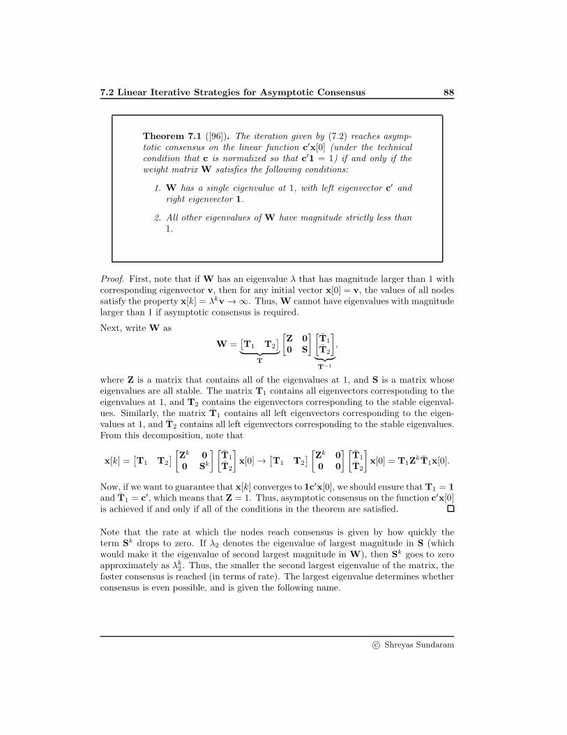
7.2 Linear Iterative Strategies for Asymptotic Consensus 88
Theorem 7.1 ([96]). The iteration given by (7.2) reaches asymp-totic consensus on the linear function c′x[0] (under the technicalcondition that c is normalized so that c′1 = 1) if and only if theweight matrix W satisfies the following conditions:
1. W has a single eigenvalue at 1, with left eigenvector c′ andright eigenvector 1.
2. All other eigenvalues of W have magnitude strictly less than1.
Proof. First, note that if W has an eigenvalue λ that has magnitude larger than 1 withcorresponding eigenvector v, then for any initial vector x[0] = v, the values of all nodessatisfy the property x[k] = λkv → ∞. Thus, W cannot have eigenvalues with magnitudelarger than 1 if asymptotic consensus is required.
Next, write W as
W =[T1 T2
]
︸ ︷︷ ︸
T
[Z 00 S
] [T1
T2
]
︸ ︷︷ ︸
T−1
,
where Z is a matrix that contains all of the eigenvalues at 1, and S is a matrix whoseeigenvalues are all stable. The matrix T1 contains all eigenvectors corresponding to theeigenvalues at 1, and T2 contains the eigenvectors corresponding to the stable eigenval-ues. Similarly, the matrix T1 contains all left eigenvectors corresponding to the eigen-values at 1, and T2 contains all left eigenvectors corresponding to the stable eigenvalues.From this decomposition, note that
x[k] =[T1 T2
][Zk 00 Sk
] [T1
T2
]
x[0] →[T1 T2
][Zk 00 0
] [T1
T2
]
x[0] = T1ZkT1x[0].
Now, if we want to guarantee that x[k] converges to 1c′x[0], we should ensure thatT1 = 1and T1 = c′, which means that Z = 1. Thus, asymptotic consensus on the function c′x[0]is achieved if and only if all of the conditions in the theorem are satisfied.
Note that the rate at which the nodes reach consensus is given by how quickly theterm Sk drops to zero. If λ2 denotes the eigenvalue of largest magnitude in S (whichwould make it the eigenvalue of second largest magnitude in W), then Sk goes to zeroapproximately as λk
2 . Thus, the smaller the second largest eigenvalue of the matrix, thefaster consensus is reached (in terms of rate). The largest eigenvalue determines whetherconsensus is even possible, and is given the following name.
c© Shreyas Sundaram

7.2 Linear Iterative Strategies for Asymptotic Consensus 89
Definition 7.4. For any square matrix A, the magnitude of thelargest eigenvalue is denoted by ρ(A), and is called the spectralradius of the matrix.
There is a large amount of literature dealing with choosing the weights in (7.2) so thatthe system reaches asymptotic consensus on a linear function [96, 61, 47, 15]. We willnow describe one such method.
7.2.1 Choosing the Weight Matrix for Asymptotic Consensus
Mathematically, the first condition in Theorem 7.1 states that W1 = 1. In other words,the sum of the elements in each row of W must be equal to 1. One way to achieve thisis to use the following concept.
Definition 7.5. Given a set of real numbers x1, x2, . . . , xn, thequantity
α1x1 + α2x2 + · · ·+ αnxn
is said to be a convex combination of x1, x2, . . . , xn if each of thescalars α1, α2, · · · , αn is nonnegative, and satisfy
∑ni=1 αi = 1.
If we have each node update its value to be a convex combination of its own and neighbors’values, then we would have wij ≥ 0 for all i, j, wij = 0 if xj /∈ Ni∪{xi}, and
∑nj=1 wij = 1
for i ∈ {1, 2, . . . , n}. This would ensure that W has an eigenvalue at 1 with eigenvector1. Note that the scheme in Example 7.1 satisfied this condition, with wij = 1
degi +1 if
xj ∈ Ni ∪ {xi}.To prove convergence, we have to show that all other eigenvalues of W are inside theunit circle. To do this, we will apply the Gersgorin Disc Theorem (see Theorem A.6 inSection A.4.4). Specifically, every diagonal element in W will be positive and less than1. Furthermore, since each row sums to 1, we have
n∑
j=1j 6=i
|wij | = 1− wii.
c© Shreyas Sundaram

7.2 Linear Iterative Strategies for Asymptotic Consensus 90
Thus, all of the Gersgorin discs are contained within the unit circle, as illustrated by thefollowing figure.
This indicates that W has no eigenvalues of magnitude larger than 1. Finally, we onlyneed to show that W has a single eigenvalue at 1. To do this, we will use the followingresult.
Lemma 7.1. If A is a square matrix with all entries positive, then A has only a singleeigenvalue of largest magnitude.
The proof of the above result requires a few other preliminary results, and so we will notcover it here. For details, see [39]. This lemma is promising, but our weight matrix Wdoes not have all elements positive (some of them are zero, corresponding to the caseswhere there is no edge between two nodes). However, under a certain condition on theunderlying network, we can indeed use this result.
Lemma 7.2. Consider a network G with n nodes, and assume that G is strongly con-nected. If all edges and self-loops are assigned a positive weight so that each row sumsto 1, then W has a single eigenvalue at 1.
Proof. Choosing the weights as specified in the Lemma, the matrix W can be viewedas the adjacency matrix for the graph G (see Section B.2 in the Appendix). Specifically,Corollary B.1 indicates that there exists some k ≤ n−1 such that all elements of Wk arepositive. Next, note that the eigenvalues of Wk are the eigenvalues of W raised to thek–th power. However, Lemma 7.1 states that the largest eigenvalue of Wk only appearsonce; thus it must be the case that the eigenvalue 1 appears only once in W.
Using the above lemma and the Gersgorin Disc Theorem, we come to the following result.
Theorem 7.2. Consider a network G with n nodes, and assumethat G is strongly connected. If all edges and self-loops are assigneda positive weight so that each row sums to 1, then all nodes in thenetwork will reach asymptotic consensus on the value c′x[0], wherec′W = c′.
c© Shreyas Sundaram

7.2 Linear Iterative Strategies for Asymptotic Consensus 91
Proof. If the conditions in the theorem are satisfied, then the Gersgorin Disc Theoremand Lemma 7.2 indicate that all conditions in Theorem 7.1 will be satisfied. Specifically,W will have a single eigenvalue at 1, with right eigenvector 1. Furthermore, all othereigenvalues will be inside the unit circle. Finally, defining c′ to be the left eigenvector ofW corresponding to the eigenvalue 1, we obtain the desired result.
Example 7.2. Let us return to the three node sensor network from Example 7.1, whereeach node updates its value to be an average of its previous value and those of itsneighbors. The weight matrix for this iteration is given by
W =
0.5 0.5 013
13
13
0 0.5 0.5
.
The network is strongly connected, and all edges and self-loops have a positive weight sothat each row sums to 1. Thus, the iteration is guaranteed to converge to consensus. Tofind what value each node converges to, we find the left eigenvector of W correspondingto eigenvalue 1 to be
c′ =[27
37
27
].
Thus, each node will converge to 27x1[0]+
37x2[0]+
27x3[0]; note that this is not guaranteed
to be the average of the initial values (which would have been 13 (x1[0] + x2[0] + x3[0]).
The reason for all nodes converging to the average in Example 7.1 is that the initialvalues were such that 2
7x1[0] +37x2[0] +
27x3[0] =
13 (x1[0] + x2[0] + x3[0]).
The above example shows that simple local averaging may not lead to consensus tothe average of all initial values, because the left eigenvector c′ of W corresponding toeigenvalue 1 may not be 1
n1′. One can guarantee convergence to the average if the sum
of all the entries in each column is also equal to 1 (so that 1n1′ is a left eigenvector of
W). To do this, suppose that the graph is undirected (i.e., the links between each nodeare bidirectional), and suppose that every node knows n. Then, if each node assigns
wij = 1nif xj ∈ Ni, wij = 0 if xj /∈ Ni, and wii = 1 − degi
n, one can verify that every
column does in fact sum to 1.
Example 7.3. In the three node network from Example 7.1, if every node applies the1nweights specified above, we obtain
W =
23
13 0
13
13
13
0 13
23
.
For this matrix, we have W1 = 1 and 1n1′W = 1
n1′, and thus all nodes will converge to
the average of any initial values.
7.2.2 Notes on Terminology
The notion of convergence to a common equilibrium value is heavily related to the conceptof a Markov Chain from probability theory. In that community, nonnegative matrices
c© Shreyas Sundaram

7.3 Linear Iterative Strategies for Secure Data Aggregation 92
where each row sums to 1 are called stochastic matrices. Furthermore, if the underlyinggraph is strongly connected, the matrix is called irreducible. If W is a nonnegativematrix and Wk is a positive matrix for some k, then W is called a primitive matrix.As shown in Corollary B.1, an irreducible matrix will be primitive if every diagonalelement is nonzero; however irreducibility by itself does not imply primitivity (as shownin Example B.4). A stochastic matrix W that converges to 1c′ for some c′ is called anergodic matrix; as shown by the proof of Theorem 7.2, any primitive stochastic matrixis ergodic. However, not all ergodic matrices need to be primitive or irreducible. Forexample, consider the stochastic matrix
W =
[0.5 0.50 1
]
.
This matrix is upper triangular, and thus Wk will also be upper triangular for anyk; therefore, the (2, 1) element will always be zero, and this matrix is not primitive.Furthermore, there is no path from the first node to the second node, so this matrix isnot irreducible. However, this matrix has only one eigenvalue at 1 (and the other is at0.5), and thus this matrix is guaranteed to converge to 1c′, where c′ is the left eigenvectorofW corresponding to eigenvalue 1 (according to Theorem 7.1). Specifically, c′ =
[0 1
],
and one can verify that
limk→∞
Wk = 1c′ =
[0 10 1
]
.
7.3 Linear Iterative Strategies for Secure Data Ag-
gregation
In the last section, we focused on using linear iterative strategies for asymptotic consensusin connected networks. In this section, we investigate the use of such strategies to treatthe problem of data accumulation in networks (where some or all nodes have to gatherall of the other values). Furthermore, we allow for the possibility that some nodes in thenetwork update their values at each time-step in an arbitrary manner, instead of followingthe predefined strategy of using a specific weighted linear combination of their neighbors’(and own) values. Such arbitrary updates can occur, for example, if some nodes inthe network are compromised by a malicious attacker whose objective is to disrupt theoperation of the network [57, 38]. Alternatively, these arbitrary updates might be theresult of hardware malfunctions at the nodes, which cause them to incorrectly calculatetheir update value [29]. Here, we will see that the graph connectivity is a determiningfactor for the ability of linear iterative strategies to tolerate malicious (or faulty) agents(see Section B.1 for a review of graph connectivity). In particular, if the connectivity ofthe graph is 2f or less, then regardless of the choice of weights in the linear iteration, it ispossible to find a subset of f (or less) nodes that can conspire to prevent some nodes fromcalculating any function of all node values. On the other hand, if the network topologyhas connectivity at least 2f +1, then any node can work around the misbehaving nodesto calculate any desired function of the initial node values, even if up to f nodes conspireand coordinate their actions in an attempt to disrupt the network. To prove these results,
c© Shreyas Sundaram
7.3 Linear Iterative Strategies for Secure Data Aggregation 93
we will exploit concepts from classical linear system theory (such as structured systemtheory, strong observability, and invariant zeros of linear systems).
In our development, we use ei to denote the column vector with a 1 in its i’th positionand 0’s elsewhere. We will also denote the cardinality (number of elements) of a set Sby |S|, and for a pair of sets S and T , we will use S \ T to denote the set of elements ofS that are not in T .
7.3.1 Attacking the Network
To start, it is useful to understand some fundamental limitations in the ability of anetwork to tolerate malicious nodes. First, as an extreme, note that if all nodes are ma-licious, there is certainly nothing that we can do. More generally, one can imagine that ifa “large” number of nodes are malicious, we would still be incapable of overcoming them.To quantify just how many malicious nodes are required to prevent data accumulationor function calculation in networks, we will study the following examples.
Example 7.4. Consider the network with three nodes from Example 7.1.
Suppose that we are going to run some algorithm A in this network so that node x1 cancalculate some function of all initial values; for instance, A could be the linear strategythat we have been studying. The algorithm is supposed to provide x1 with enoughinformation about x2 and x3’s values to be able to calculate the function. However,all information that x1 receives about x3 comes through x2. However, suppose x2 ismalicious and decides to pretend that x3’s value is something that it is not; x2 will runthe algorithm A with this false value of x3. In this case, x1 would never be able to tellthat x2 is lying, because it has no other way to receive information about x3’s value, andthus it has no choice but to trust x2. Thus, x2 can prevent x1 from correctly calculatingits desired function.
Example 7.5. Consider the following network with four nodes.
Once again, x1 wants to calculate some function of all initial values via some algorithmA. However, suppose now that node x3 is malicious, and will pretend that node x4’svalue is something that it is not. However, node x2 will run correctly, and use x4’s truevalue in the algorithm. In this case, the only way that information about x4 gets to nodex1 is through x2 and x3. However, due to x3’s duplicitous behavior, the information that
c© Shreyas Sundaram

7.3 Linear Iterative Strategies for Secure Data Aggregation 94
x1 receives about x4 will be inconsistent. Furthermore, node x1 has no a priori reasonto believe x2 over x3, or vice versa. Thus, x3 can prevent x1 from ever finding the truevalue of x4.
Both of the above examples demonstrate that networks can be disrupted by a small andcarefully chosen set of malicious nodes. The key observation is that the malicious nodesacted as a gateway for information between two sets of non-malicious nodes. This canbe formally captured by the notion of a vertex cut in the graph; recall that a vertex cutis a set of nodes that removes all paths from one group of nodes to another group ofnodes (see Section B.1). Using the intuition from the above examples, we can state thefollowing result.
Theorem 7.3. For a given network G, let κij denote the size of thesmallest (i, j)-cut between nodes xi and xj. If κij ≤ 2f , then thereis a choice of f malicious nodes that can prevent node xj fromcalculating any function of xi’s value, regardless of the algorithmthat is used in the network.
Proof. Given any nodes xi and xj , let Sij denote the (i, j)-cut with size κij . For thepurposes of this proof, assume that xi is not a neighbor of xj (because otherwise, thereis no vertex cut that removes all paths from xi to xj). All information about xi must gothrough the nodes in Sij to reach xj . Suppose that half of the nodes in Sij are malicious,and decide to run the algorithm pretending that xi’s value is something that it is not.Now the information that xj receives from the algorithm is inconsistent, and xj wouldnot know which half of the vertex cut to trust. Since the cut was chosen to have sizeκij ≤ 2f , there are at most f malicious nodes that are required in order to disrupt thenetwork in this way.
7.3.2 Modeling Malicious Nodes in the Linear Iterative Strategy
The previous section showed that the connectivity of the network must be at least 2f+1in order to tolerate any f malicious nodes, regardless of the algorithm. We now look atthe question: can the linear iterative strategy be used to overcome f malicious nodes innetworks of connectivity 2f + 1? We will answer this question in the affirmative, butfirst, we need to mathematically model malicious behavior in the context of the linearstrategy.
To this end, suppose that instead of applying the update equation (7.1), some node xl
updates its value at each time-step as
xl[k + 1] = wllxl[k] +∑
j∈Nl
wljxj [k] + ul[k] , (7.3)
where ul[k] is an additive error at time-step k.
c© Shreyas Sundaram

7.3 Linear Iterative Strategies for Secure Data Aggregation 95
Definition 7.6. Suppose all nodes run the linear iteration for T time-steps in orderto perform function calculation. Node xl is said to be malicious (or faulty) if ul[k] isnonzero for at least one time-step k, 0 ≤ k ≤ T − 1.
Note that the model for malicious nodes considered here is quite general, and allows nodexl to update its value in a completely arbitrary manner (via appropriate choices of ul[k]at each time-step). As such, this model encapsulates a wide variety of malicious behavior(including a conspiracy by a set of malicious nodes). It is worth noting that we do nottreat the case where nodes try to influence the result of the computation by modifyingtheir initial values (because of the philosophically different nature of this problem). Wewill show that our protocol allows every node to obtain every initial value (maliciouslymodified or not), and so one can potentially handle corrupted initial values by havingeach node use some sort of statistical analysis to detect and discard suspicious initialvalues. This is also a non-issue when the desired function only involves initial valuesfrom some trusted nodes, but intermediate (routing) nodes can be malicious.
Let F = {xi1 , xi2 , . . . , xif } denote the set of nodes that are malicious during a run ofthe linear iteration. Using (7.2) and (7.3), the linear iteration can then be modeled as
x[k + 1] = Wx[k] +[ei1 ei2 · · · eif
]
︸ ︷︷ ︸
BF
ui1 [k]ui2 [k]
...uif [k]
︸ ︷︷ ︸
uF [k]
yi[k] = Cix[k], 1 ≤ i ≤ n ,
(7.4)
where yi[k] represents the outputs (node values) seen by node i during time-step k ofthe linear iteration. Specifically, Ci is a (degi+1) × n matrix with a single 1 in eachrow capturing the positions of the state-vector x[k] that are available to node xi (thesepositions correspond to neighbors of node xi, along with node xi itself). Recall that eldenotes a unit vector with a single nonzero entry with value 1 at its l’th position.
Example 7.6. Consider the three node network from Example 7.1. Since node x1
receives its own value and x2’s value at each time-step, we can write
y1[k] =
[1 0 00 1 0
]
︸ ︷︷ ︸
C1
x[k].
Note that (7.4) is a linear system with unknown inputs (since xi does not know the faultscaused by the malicious nodes). However, there is one other aspect of this system thatis unknown to xi: the set of malicious nodes F , and thus the exact matrix BF . If thismatrix were known, recovering all initial values via the linear iteration would reduce tothe problem of strong observability of the above system (see Section 2.6.4). As we willsee later, the fact that we do not know BF will require us to consider strong observabilityof a slightly different system in order to allow xi to recover all initial values.
c© Shreyas Sundaram

7.3 Linear Iterative Strategies for Secure Data Aggregation 96
As in Section 2.6.2, the set of all values seen by node i during the first L+ 1 time-stepsof the linear iteration is given by
yi[0]yi[1]yi[2]...
yi[L]
︸ ︷︷ ︸
yi[0:L]
=
Ci
CiWCiW
2
...CiW
L
︸ ︷︷ ︸
Oi,L
x[0] +
0 0 · · · 0CiBF 0 · · · 0
CiWBF CiBF · · · 0...
.... . .
...CiW
L−1BF CiWL−2BF · · · CiBF
︸ ︷︷ ︸
JF
i,L
uF [0]uF [1]uF [2]
...uF [L− 1]
︸ ︷︷ ︸
uF [0:L−1]
.
(7.5)
The matrices Oi,L and J Fi,L characterize the ability of node xi to calculate the required
function of the initial values. The matrix Oi,L is the observability matrix for the pair(W,Ci), and J F
i,L is the invertibility matrix for the system (W,BF ,Ci).
7.3.3 Calculating Functions in the Presence of Malicious Nodes
when κ ≥ 2f + 1
First, suppose that there are at most f malicious nodes in the network, given by the setF . From the perspective of any node xi, the linear iteration has the form of the linearsystem in (7.4). As explained in Section 7.3.2, if F were known, this would simply be aproblem of strong observability of the system. However, since F is unknown, a little moreanalysis is needed. Essentially, we would like to be able to uniquely identify the initialstate of the system (7.4) from the outputs, regardless of the set F of f malicious nodes.In other words, we want to ensure that two different initial states and two different setsof f malicious nodes cannot produce the same outputs for all time. With this intuition,the following theorem presents the condition required for recovering the initial valuesdespite any unknown set of f malicious nodes.
Theorem 7.4. Suppose there exists a weight matrix W (with wij = 0 if xj /∈ Ni∪{xi})such that for any set S of 2f nodes, the system
x[k + 1] = Wx[k] +BSuS [k]
yi[k] = Cix[k]
is strongly observable. Then node xi can uniquely recover all initial values after at mostN time-steps of the linear iteration, despite the actions of any unknown set of f maliciousnodes.
Note that the above theorem requires us to consider strong observability of a systemwith 2f nodes in order to overcome f malicious nodes – this is the price paid for notknowing the set of malicious nodes a priori.
Proof. We will show that if the condition in the theorem is satisfied, then the outputof (7.4) can be generated by only one initial condition. We will prove by contradiction:
c© Shreyas Sundaram

7.3 Linear Iterative Strategies for Secure Data Aggregation 97
suppose that there is an initial condition x[0] 6= x[0] and some set Fc of f maliciousnodes (perhaps different from F) that causes the linear iteration to produce the sameoutput values as the original linear iteration for all time. The linear iteration for thisdifferent configuration is given by
x[k + 1] = Wx[k] +BFcuFc
[k]
yi[k] = Cix[k].
Since, by assumption, the output of this system is the same as the output of (7.4) forall k, we have
Cix[k] = Cix[k] ⇔ Ci(x[k]− x[k]) = 0 ∀k ∈ N. (7.6)
Define x[k] = x[k]− x[k], so that
x[k + 1] = Wx[k] +BFuF [k]−Wx[k]−BFc[k]
= Wx[k] +[BF BFc
]
︸ ︷︷ ︸
BF∪Fc
[uF [k]
−uFc[k]
]
︸ ︷︷ ︸
uF∪Fc [k]
. (7.7)
This defines a linear system with initial condition x[0] 6= 0 (since x[0] 6= x[0]). How-ever, (7.6) indicates that Cix[k] = 0 for all k ∈ N, which indicates that the system(W,BF∪Fc
,Ci,0) is not strongly observable. However, since each of F and Fc have atmost f nodes each, F ∪ Fc has at most 2f nodes; thus, we reach a contradiction, sincethe assumption in the theorem is that the system with any set of 2f nodes is stronglyobservable.
Thus, if the system (W,BS ,Ci,0) is strongly observable for any set S of 2f nodes,the outputs of the linear iteration will uniquely specify the initial values despite theactions of any f malicious nodes. Furthermore, since strong observability implies thatthe outputs of the system over N time-steps are sufficient to recover the initial state,we see that node xi can obtain all initial values after running the linear iteration for atmost N time-steps.
The above result says that if the system (W,BS ,Ci,0) is strongly observable for anyset S of 2f nodes, node xi can recover x[0] after viewing its neighbors’ (and own) valuesover at most N time-steps, despite the actions of any set F of f malicious nodes. To seeexactly how xi can do this, note that the set of all values seen by xi over N time-stepsis given by
yi[0 : N ] = Oi,Nx[0] + J Fi,NuF [0 : N − 1].
Node xi does not know x[0], uF [0 : N−1] and the set F ; Suppose now that xi simply tries
to find a set Fc of f nodes such that yi[0 : L] is in the range of the matrix[
Oi,L J Fc
i,L
]
,
i.e.,yi[0 : L] = Oi,Lx[0] + J Fc
i,L u
for some vectors x[0] and u. Since the output of the system can only have been generatedby one particular state, the only way for xi to write its values in this way is if x[0] = x[0]
c© Shreyas Sundaram

7.3 Linear Iterative Strategies for Secure Data Aggregation 98
– thus, xi has recovered all initial values. Note that checking for all(Nf
)possibilities when
trying to determine the possible set Fc of malicious nodes is equivalent to the brute forcemethod of determining up to f errors in an N -dimensional real number codeword withdistance 2f + 1. In the coding theory literature, there exist efficient ways of performingthis check for both structured and random real number codes (e.g., see [86] and thereferences therein), and one can potentially exploit those results to streamline the abovedecoding procedure. This is an open problem for research.
Next, we will show that when κ ≥ 2f + 1, one can find a weight matrix W so that(W,BS ,Ci,0) is strongly observable for any set S of up to 2f nodes.
Invariant Zeros
Recall from Section 2.9.3 that for any set S ⊂ X of 2f nodes, the matrix
P(z) =
[W − zIn BS
Ci 0
]
is called the matrix pencil for the system (W,BS ,Ci,0). Furthermore, any z ∈ C forwhich
rank (P(z)) < n+ 2f
is called an invariant zero of the system, and the system (W,BS ,Ci,0) will be stronglyobservable if and only if it has no invariant zeros. We will now focus on choosing W(with the required sparsity constraints) so that the system has no invariant zeros forany set S ⊆ X of 2f nodes. Note that the assumption that the number of outputs islarger than the number of inputs will be trivially satisfied in networks that have (2f+1)-connectivity, because each node i will have at least 2f + 1 neighbors, and thus Ci willhave at least 2f + 2 rows.
Let S = {xi1 , xi2 , . . . , xi2f } denote any set of 2f nodes, and let S = X \ S. Define
BS =[ei1 ei2 · · · ei2f
]. For any choice of weights for the linear iteration, let WS
represent the weight matrix corresponding to interconnections within the set S, WS,S
represent the weight matrix corresponding to connections from the set S to the set S,WS represent the weight matrix corresponding to interconnections within the set S, andWS,S represent the weight matrix corresponding to connections from the set S to the setS. Note that WS has dimension (n−2f)× (n−2f), and WS has dimension (2f)× (2f).Furthermore, for any node xi, let
[Ci,S Ci,S
]denote a (degi +1) × n matrix with a
single 1 in each row corresponding to the nodes in X that are neighbors of node xi, alongwith node xi itself (the first n − 2f columns correspond to nodes in S and the last 2fcolumns correspond to nodes in S).
Lemma 7.3. For any set S of 2f nodes, the invariant zeros of (W,BS ,Ci,0) are exactlythe invariant zeros of (WS ,WS,S,Ci,S ,Ci,S).
Proof. Without loss of generality, we can assume that W is of the form
W =
[WS WS,S
WS,S WS
]
,
c© Shreyas Sundaram

7.3 Linear Iterative Strategies for Secure Data Aggregation 99
since this is obtained simply by renumbering the nodes so that nodes in the set S haveindices between n − 2f + 1 and n. This also means that BS has the form BS =
[0I2f
],
and P(z) can be written as
P(z) =
WS − zIn−2f WS,S 0WS,S WS − zI2f I2fCi,S Ci,S 0
.
From this expression, we see that
rank(P(z)) = 2f + rank
([WS − zIn−2f WS,S
Ci,S Ci,S
])
,
and so the invariant zeros of the set (W,BS ,Ci,0) are exactly the invariant zeros of theset (WS ,WS,S,Ci,S ,Ci,S).
Lemma 7.3 reveals that in order to ensure that the system (W,BS ,Ci,0) is stronglyobservable for every set S of 2f nodes and every node xi, we can focus on the problemof choosing the weight matrix W so that the set (WS ,WS,S,Ci,S ,Ci,S) will have noinvariant zeros, for any choice of i and for any set S of 2f nodes. The tricky part isthat the weight matrix is structured, and we will somehow have to relate the invariantzeros of the system to the zero/nonzero constraints in W. To accomplish this, we willuse techniques from a branch of control theory pertaining to linear structured systems[66, 18]. See Appendix C for an overview of some of the main concepts from structuredsystem theory.
Application to Secure Information Dissemination
To apply structured system theory to the problem of determining the number of invariantzeros of the set (WS ,WS,S,Ci,S ,Ci,S), we note that all matrices in this set are essentiallystructured matrices, with the exception that the nonzero entries in Ci,S and Ci,S aretaken to be 1 rather than free parameters. However, this is easily remedied by defining thematrix Λi = diag
(λi,1, λi,2, · · · , λi,degi +1
), where the λi,j ’s are a set of free (independent)
parameters. Now consider the matrix[Ci,S Ci,S
]= Λi
[Ci,S Ci,S
]. The nonzero
entries in the matrices Ci,S and Ci,S are thus independent free parameters (at mostone per row in each matrix), and these matrices therefore qualify as valid structuredmatrices. Now consider the matrix pencil
P(z) =
[WS − zIn−2f WS,S
Ci,S Ci,S
]
=
[In−2f 00 Λi
] [WS − zIn−2f WS,S
Ci,S Ci,S
]
.
If the matrix Λi is invertible, the matrix pencil for the set (WS ,WS,S, Ci,S , Ci,S) willhave the same rank as the matrix pencil for the set (WS ,WS,S,Ci,S ,Ci,S) for all z ∈ C.Thus, for the purposes of analyzing the number of invariant zeros of the system, we canassume without loss of generality that the nonzero entries in Ci,S and Ci,S are all ones(i.e., we can take Λi to be the identity matrix).
c© Shreyas Sundaram

7.3 Linear Iterative Strategies for Secure Data Aggregation 100
Let us start by defining the graph H associated with the set (WS ,WS,S,Ci,S ,Ci,S).For this set of matrices, note that the state vertices in the graph H are given by theset S, and the input vertices are given by the set S; thus the graph has n − 2f statevertices and 2f input vertices. In particular, H can be obtained by first taking the graphof the network G, and removing all incoming edges to nodes in S (since the nodes in Sare treated as inputs in the above set of matrices). To this graph, add degi +1 outputvertices (denoted by the set Yi), and place a single edge from the set xi ∪Ni to verticesin Yi, corresponding to the single nonzero entry in each row of the matrices Ci,S andCi,S . Furthermore, add a set of self loops to every state vertex to correspond to thenonzero entries on the diagonal of the weight matrix WS .
We can now use the above results on structured systems to prove the following lemma forthe linear iteration in (7.4). We will then use this lemma, in conjunction with Lemma 7.3and Theorem 7.4, to show that all nodes will be able to uniquely determine the vectorx[0] after running the linear iteration for at most n time-steps (with up to f maliciousnodes).
Lemma 7.4. Let the graph of the network G have connectivity κ. Let xi be any node inthe network, and let S be any set of 2f nodes. If κ ≥ 2f +1, then for almost any choiceof weights, the set (WS ,WS,S,Ci,S ,Ci,S) will have no invariant zeros.
Proof. We will show that the matrix pencil
[WS − zIn−2f WS,S
Ci,S Ci,S
]
has full normal-rank (equal to n) even after the deletion of an arbitrary row. We willthen use Theorem C.6 to prove the lemma.
Suppose we remove one of the rows of P(z) corresponding to a vertex v ∈ S (i.e., oneof the top n − 2f rows of P(z)), and denote the resulting matrix by P(z). Note thatremoving this row is equivalent to removing all incoming edges to vertex v in H; however,all outgoing edges from v are still left in the graph (since the column corresponding tovertex v is left in matrix P(z)). Thus, if we denote the resulting graph (after removingthe incoming edges to v in H) by H, we see that vertex v can be treated as an inputvertex in H. Since the set S ∪ v has size 2f + 1, and since the graph G of the networkhas connectivity κ ≥ 2f +1, Theorem B.2 says that there will be a linking of size 2f +1from the set S ∪ v to the set xi ∪ Ni in G, and hence in H (since such a linking wouldnot use any incoming edges to vertex v). From Theorem C.2, the matrix pencil P(z)will thus have rank equal to (n− 2f − 1)+ 2f +1 = n for almost any choice of W, evenafter the deletion of the row of corresponding to any vertex v ∈ S.
Now, instead of removing one of the first n − 2f rows, suppose we remove one of therows of P(z) corresponding to one of the output vertices in Yi (i.e., one of the bottomdegi+1 rows of P(z)). Since degi+1 ≥ κ + 1 ≥ 2f + 2, removing one of the outputvertices leaves at least 2f + 1 output vertices in the graph H. Choose any 2f of thenodes in xi ∪Ni such that none of the chosen nodes have an edge to the removed outputvertex in H (this is possible since each output vertex only connects to a single vertex in
c© Shreyas Sundaram

7.3 Linear Iterative Strategies for Secure Data Aggregation 101
xi ∪ Ni). Denote these 2f nodes by Xi. Once again, since the graph is at least 2f + 1connected, there exists a linking of size 2f from S to Xi, and therefore to the remainingoutput vertices in the graph H. From Theorem C.2, the matrix pencil will have rankequal to (n− 2f) + 2f = n for almost any choice of W, even after the deletion of one ofthe bottom degi+1 rows of P(z)).
The above arguments show that P(z) will generically have full column rank after thedeletion of an arbitrary row. From Theorem C.6, the number of invariant zeros of P(z)is equal to n− 2f minus the maximal number of vertices in S contained in the disjointunion of a size 2f linking from S to Yi, a cycle family in S, and a Yi-topped path family.If we simply take all the self-loops in H (corresponding to the nonzero weights on thediagonal of the weight matrix WS), we will have a set of disjoint cycles that covers alln − 2f vertices in S. Thus, the matrix pencil P(z) will generically have no invariantzeros, thereby proving the lemma.
With the above lemma in hand, one can now prove the following result.
Theorem 7.5. Let f denote the maximum number of maliciousnodes that are to be tolerated in a given network G, and let κ denotethe connectivity of the network. If κ ≥ 2f + 1, then for almost anychoice of weight matrix, every node in the network can calculate anyfunction of the initial values after running the linear iteration forat most n time-steps, even when there are up to f malicious nodesthat update their values arbitrarily (and possibly in a coordinatedmanner) at each time-step.
Proof. From Lemmas 7.3 and 7.4, we see that for almost any choice of weight matrixW (satisfying the required sparsity constraints), the set (W,BS ,Ci,0) will have noinvariant zeros, for any xi and any set S of 2f nodes. Furthermore, since the set ofweights for which this property does not hold lies on an algebraic variety (i.e., it holdsfor almost any choice of weights), it will hold generically (and therefore simultaneously)for all xi and for all possible sets S of 2f nodes. Thus, Theorem 7.4 is satisfied for all xi,and every node can calculate any arbitrary function of the initial values after runningthe linear iteration for at most n time-steps, despite the actions of up to f maliciousnodes.
Remark 7.1. The above results were derived in [83, 84, 85]. Extensions of these resultsto the case where some nodes are faulty but not malicious (i.e., nodes that do not injectthe worst-case inputs into the system), and where the objective is to reach consensus inthe network, were performed in [62], using ideas similar to the fault-diagnosis schemescovered in Chapter 4.
c© Shreyas Sundaram

Appendix A
Linear Algebra
A.1 Fields
A field F is a set of elements, together with two operations written as addition (+) andmultiplication (×),1 satisfying the following properties [22]:
1. Closure: a+ b ∈ F and ab ∈ F for all a, b ∈ F.
2. Commutativity: a+ b = b+ a and ab = ba for all a, b ∈ F.
3. Associativity: (a+ b) + c = a+ (b+ c) and (ab)c = a(bc) for all a, b, c ∈ F.
4. Distributivity: a(b+ c) = ab+ ac for all a, b, c ∈ F.
5. Additive identity: There exists an element 0 ∈ F such that for all a ∈ F, a+0 = a.
6. Multiplicative identity: There exists an element 1 ∈ F such that for all a ∈ F,1a = a.
7. Additive inverse: For each element a ∈ F, there exists an element d ∈ F such thata+ d = 0.
8. Multiplicative inverse: For each nonzero element a ∈ F, there exists an elemente ∈ F such that ae = 1.
The number of elements in a field can be infinite (such as in the field of real or complexnumbers), or finite. We will be dealing only with fields of infinite size in this course.
1The multiplicative operator is also frequently denoted by simply concatenating the operands (i.e.,a× b is written as ab). We will adopt this convention throughout the discussion.
c© Shreyas Sundaram

A.2 Vector Spaces and Subspaces 103
A.2 Vector Spaces and Subspaces
A vector space V over a field F (denoted as (V,F)) is a set of elements V, together withtwo operations written as addition (+) and multiplication (×), satisfying the followingproperties:
1. Closure under addition: x+ y ∈ V for all x,y ∈ V.
2. Closure under scalar multiplication: ax ∈ V for all x ∈ V and a ∈ F.
3. Commutativity of addition: x+ y = y + x for all x,y ∈ V.
4. Associativity of addition: (x+ y) + z = x+ (y + z) for all x,y, z ∈ V.
5. Additive identity: There exists an element 0 ∈ V such that for all x ∈ V, x+0 = x.
6. Additive inverse: For each x ∈ V, there exists an element y ∈ V such thatx+ y = 0.
7. Multiplication by scalar identity: For all x ∈ V, the multiplicative identity 1 inthe field F satisfies 1x = x.
8. Associativity under scalar multiplication: For all a, b ∈ F and for all x ∈ V,(ab)x = a(bx).
9. Distributivity of scalars: For all a, b ∈ F and for all x,y ∈ V, a(x+ y) = ax+ ayand (a+ b)x = ax+ bx.
The elements of V are called vectors and the elements of F are called scalars. As doneabove, we will denote vectors with a boldface character x ∈ V, and scalars in the usualtypeface a ∈ F.
A subspace of a vector space (V,F) is a subset W ⊆ V such that (W,F) is a vector spacewith the operations of addition and multiplication defined above.
Although the term vector refers to any element of a set V satisfying the above vectorspace properties, we will most commonly encounter vectors in the following sense. Forany elements a1, a2, . . . , an ∈ F, define the column vector
a =
a1a2...an
.
The set of all column vectors of the above form is denoted by Fn, and is a vector space overthe field F. The operations of addition and multiplication by scalars in this vector space
c© Shreyas Sundaram

A.3 Linear Independence and Bases 104
are done on a component by component basis, i.e., for any a1, a2, . . . , an, b1, b2, . . . , bn, b ∈F,
a1a2...an
+
b1b2...bn
=
a1 + b1a2 + b2
...an + bn
, b
a1a2...an
=
ba1ba2...
ban
.
Alternatively, one can define a row vector
a =[a1 a2 · · · an
],
with the operations of addition and multiplication defined in an analogous manner.
A.3 Linear Independence and Bases
Given a vector space (V,F), a set of vectors v1,v2, . . . ,vr ∈ V are said to be linearlyindependent if the only set of scalars a1, a2, . . . , ar ∈ F satisfying the equation
a1v1 + a2v2 + · · ·+ arvr = 0
is a1 = a2 = · · · = ar = 0. Otherwise, the vectors are said to be linearly dependent.Note that if a set of vectors are not linearly independent, then one of the vectors can bewritten as a linear combination of the other vectors.
Let B = {v1,v2, . . . ,vr} be a set of linearly independent vectors of maximal size in thevector space (V,F). The set B is called a basis for the vector space. The following resultholds.
Theorem A.1. Any vector in the vector space (V,F) can be writtenas a linear combination of the vectors in B.
Proof. Consider any vector v ∈ V. Since B is a linearly independent set of maximal size,it must be the case that there is a nontrivial solution a, a1, a2, . . . , ar to the equation
av + a1v1 + a2v2 + · · ·+ arvr = 0;
otherwise, the set {v,v1,v2, . . . ,vr} is a set of linearly independent vectors that is largerthan B. Next, note that it must be the case that a 6= 0, since otherwise, there would bea nontrivial linear combination of the vectors in B that sum to zero, contradicting theassumption of a linearly independent set. Thus, we can write
v = −a1av1 −
a2av2 − · · · − ar
avr,
proving the above statement.
c© Shreyas Sundaram

A.4 Matrices 105
Theorem A.2. Let B1 and B2 be two different bases for a vectorspace (V,F). Then |B1| = |B2|.
The proof of the above result can be found in [22]. In words, the above result says thatall bases for a vector space are comprised of the same number of vectors. The size of anybasis for a vector space (V,F) is called the dimension of the vector space, and is denotedby dim(V).
A.4 Matrices
An m× n matrix A over a field F is a rectangular array of elements from F, depicted as
A =
a11 a12 · · · a1na21 a22 · · · a2n...
.... . .
...am1 am2 · · · amn
.
When m = n, the matrix is said to be square. Note that a column vector is a matrixwith n = 1 and a row-vector is a matrix with m = 1. The set of all m× n matrices overa field F is denoted by Mm,n(F). Each column of an m× n matrix can be viewed as anelement of the vector space (Fm,F), and each row can be viewed as an element of thevector space (Fn,F). The element in row i and column j of a matrix A is denoted by aij .For a vector a ∈ Mn,1(F), the i–th component is simply denoted as ai. The transposeof an m× n matrix A is the n×m matrix obtained by converting each of the columnsinto rows, and is denoted by
A′ =
a11 a21 · · · am1
a12 a22 · · · am2
......
. . ....
a1n a2n · · · amn
.
With this notation, row vectors will usually be denoted as the transpose of a columnvector (i.e., a is a column vector and a′ is a row vector).
The inner product of two column vectors a,b ∈ Mn,1 is defined as
a′b ,
n∑
k=1
akbk.
The product of two matrices A ∈ Mm,n(F) and B ∈ Mp,q(F) is defined if and only ifn = p, and produces a matrix C ∈ Mm,q(F). Entry (i, j) in matrix C = AB is obtained
c© Shreyas Sundaram

A.4 Matrices 106
as
cij =
n∑
k=1
aikbkj .
A square n × n matrix A is said to be diagonal if all entries except a11, a22, . . . , annare zero. An n × n diagonal matrix with a11 = a22 = · · · = ann = 1 is called theidentity matrix, and is denoted by In. Note that for any matrix A ∈ Mn,m(F), we haveImA = AIn = A. A matrix is said to be upper-triangular if all entries below the maindiagonal are zero, and lower-triangular if all entries above the main diagonal are zero.
The rank of a matrix A ∈ Mm,n(F) is defined as the maximum number of linearlyindependent columns in that matrix, and is denoted by rank(A). The following resultsare fundamental (see [22] for proofs).
Theorem A.3. Given a matrix A ∈ Mm,n(F):
1. rank(A) = rank(A′).
2. rank(A) ≤ min(m,n).
3. For any matrices B ∈ Mp,m(F) and C ∈ Mn,q(F),
rank(BAC) ≤ min(rank(A), rank(B), rank(C)).
4. For any matrices B ∈ Mp,m(F) and C ∈ Mn,q(F) satisfyingrank(B) = m and rank(C) = n, rank(BAC) = rank(A).
The first identity in the above list is of particular importance. Since the columns ofA′ are simply the rows of A, this identity says that the maximum number of linearlyindependent columns in A is equal to the maximum number of linearly independent rowsin A.
A matrix A ∈ Mm,n(F) is said to be full-column-rank if rank(A) = n, and full-row-rank if rank(A) = m. A full-column-rank matrix is also called nonsingular. A squarematrix that is full-column-rank (or equivalently full-row-rank) is said to be nonsingular orinvertible. For every invertible matrix A ∈ Mn,n(F), there is another invertible matrix,denoted A−1 ∈ Mn,n(F) such that
AA−1 = A−1A = I.
A.4.1 Linear transformations, Range space and Null Space
Given a matrix A ∈ Mm,n(F) and a vector x ∈ Fn, the product Ax is a vector in Fm.Thus the matrix A can be viewed as a mapping or transformation from the vector space
c© Shreyas Sundaram

A.4 Matrices 107
(Fn,F) to the vector space (Fm,F). More specifically, it is a linear mapping because itsatisfies the Principle of Superposition:
A(α1x1 + βx2) = αAx1 + βAx2, ∀α, β ∈ F, ∀x1,x2 ∈ Fn.
The range space (also known as the column space or image) of the linear transformationA is defined as
R(A) , {y ∈ Fm | y = Ax for some x ∈ F
n},and the null space (or kernel) of A is defined as
N (A) , {x ∈ Fn | Ax = 0}.
One can readily verify that R(A) and N (A) are, in fact, subspaces of Fm and Fn,respectively. Since every vector in the space R(A) is a linear combination of the columnsof A, we see that a maximal set of linearly independent columns from A forms a basisfor R(A). Furthermore, dim(R(A)) = rank(A).
The dimension of the null space ofA is called the nullity ofA. The following fundamentalresult relates the rank and nullity of a linear transformation A.
Theorem A.4. For any matrix A ∈ Mm,n(F), dim(R(A)) +dim(N (A)) = n.
Proof. Suppose that the dimension of N (A) is k, and let v1,v2, . . . ,vk form a basis forthis space. Let vk+1,vk+2, . . . ,vn be any set of k − n vectors such that v1, . . . ,vn is alinearly independent set; this set spans the entire space Fn. Now consider any vector yin the range space of A, and note that by the definition of the range space,
y = Ax = A (α1v1 + α2v2 + · · ·+ αnvn)
= A (αk+1vk+1 + αk+2vk+2 + · · ·+ αnvn)
for some scalars α1, . . . , αn (this is because any vector x ∈ Fn can be written as a linearcombination of the vectors v1, . . . ,vn). The last line in the above expression follows sincev1, . . . ,vk are in the null space of A. Thus, the vectors Avk+1,Avk+2, . . . ,Avn spanthe range space of A (i.e., any vector in R(A) can be written as a linear combinationof those vectors). It only remains to show that these vectors are linearly independent,and thus are indeed a basis. To do this, suppose that there is some nontrivial linearcombination of Avk+1,Avk+2, . . . ,Avn that is equal to zero, i.e.,
βk+1Avk+1 + βk+2Avk+2 + · · ·+ βnAvn = 0
for some scalars βk+1, . . . , βn. By pulling out A on the left, this is equivalent to sayingthat the vector βk+1vk+1 + · · ·βnvn is in the null space of A, or equivalently that
βk+1vk+1 + · · ·βnvn = γ1v1 + γ2v2 + · · ·+ γkvk
c© Shreyas Sundaram

A.4 Matrices 108
for some scalars γ1, . . . , γk (again, because v1, . . . ,vk form a basis for the null space ofA). But this would mean that there is a nontrivial linear combination of v1,v2, . . . ,vn
that is equal to zero, and this is not possible by the fact that these vectors were chosento be linearly independent. Thus, it must be the case that Avk+1,Avk+2, . . . ,Avn arelinearly independent, and do indeed form a basis for the range space of A. This showsthat dim(R(A)) = n− k, and so dim(R(A)) + dim(N (A)) = n.
One can also speak of the row space of a given matrix A ∈ Mm,n(F), which is the spacespanned by the rows of A. Similarly, the left null space of A is the set of all row vectorsx ∈ Fm such that xA = 0.
A.4.2 Systems of Linear Equations
Given a matrix A ∈ Mm,n(F) and a vector y ∈ Fm, we will often be interested in solvinga linear equation of the form
y = Ax
for the vector x ∈ Fn. First, note that there exists such a vector if and only if y ∈ R(A).However, this does not mean that there will be a unique solution for x. Specifically,consider any solution x, and consider any vector n ∈ N (A). ThenA(x+n) = Ax+An =y + 0 = y, and so x + n is also a feasible solution. Thus, if the null space of A is non-empty (i.e., A is not full-column-rank), then there will be an infinite number of solutionsto the equation. The following lemma shows the converse result, and also demonstratesan important proof method.
Lemma A.1. Let A be a nonsingular matrix (i.e., all of itscolumns are linearly independent). Then there is a unique solutionx to the equation Ax = y, for any vector y.
Proof. Suppose that there were, in fact, two different solutions x1 and x2. This wouldmean that y = Ax1 = Ax2, which in turn means that A(x1 − x2) = 0. Thus, x1 − x2
is in the null space of A, which is empty due to the fact that A is nonsingular. Thusx1 − x2 = 0, which produces the desired contradiction.
The above argument is in the form of a proof by contradiction. This is an extremelyeffective proof technique, and very commonly used:
Reductio ad absurdum, which Euclid loved so much, is one of a mathemati-cian’s finest weapons. It is a far finer gambit than any chess gambit: a chessplayer may offer the sacrifice of a pawn or even a piece, but a mathematicianoffers the game. – G. H. Hardy [34]
c© Shreyas Sundaram

A.4 Matrices 109
A.4.3 Determinants
The determinant is a function that maps a square matrix A ∈ Mn,n(F) to a scalar valuein the field F. For n = 2, the determinant is given by
det
([a11 a12a21 a22
])
= a11a22 − a21a22.
Determinants of higher order matrices can be defined recursively using the followingLaplace expansion. First, for n = 1, the determinant of the matrix is defined to be thesingle scalar element comprising that matrix. For n ≥ 2, let Aij denote the (n−1)×(n−1)matrix that is obtained by removing row i and column j from matrix A. Then, for any1 ≤ i ≤ n,
det(A) =
n∑
j=1
(−1)i+jaij det(Aij).
This expansion will yield the same result for det(A) no matter which row i is used.Alternatively, the expansion can be performed around any column, yielding the sameresult. For example, for n = 3 and with i = 1, we have
det
a11 a12 a13a21 a22 a23a31 a32 a33
= a11 det
([a22 a23a32 a33
])
− a12 det
([a21 a23a31 a33
])
+ a13 det
([a21 a22a31 a32
])
= a11a22a33 − a11a23a32 + a12a23a31 − a12a21a33
+ a13a21a32 − a13a22a31.
Taking a closer look at the above determinants, we see the following.
The determinant of a matrix A ∈ Mn,n(F) is a polynomial inthe elements aij . Each term in the polynomial is a product ofn elements, no two of which are from the same row or column ofA. Furthermore, each of these products is multiplied by either +1or −1.
An immediate consequence of the above definitions is that the determinant of an upper-triangular or a lower-triangular matrix is simply the product of the elements on thediagonal. Some other important properties of determinants are summarized below (see[39] for proofs).
c© Shreyas Sundaram

A.4 Matrices 110
Theorem A.5. Given matrices A,B ∈ Mn,n(F):
1. det(A) = 0 if and only if rank(A) < n.
2. det(A) = det(A′).
3. det(AB) = det(A) det(B).
4. If A is invertible, then det(A−1) = 1det(A) .
A.4.4 Eigenvalues and Eigenvectors
An element λ ∈ F is called an eigenvalue of a square matrix A ∈ Mn,n(F) if there existsa vector v ∈ F
n such thatAv = λv .
The vector v is called the eigenvector corresponding to the eigenvalue λ. To furthercharacterize the eigenvalues of a given matrix A, one can rearrange the above equationto obtain (λIn −A)v = 0. This indicates that any eigenvalue-eigenvector pair λ and vmust be such that v lies in the null space of the matrix λIn−A. Recall from Theorem A.5in Section A.4.3 that the matrix λIn −A will have a nontrivial null space if and only ifdet(λIn −A) = 0. Next, since the determinant of a matrix is simply a polynomial in theelements of that matrix, we see that
det(λIn −A) = λn + pn−1λn−1 + pn−2λ
n−2 + · · ·+ p1λ+ p0 , (A.1)
where p0, p1, . . . , pn−1 are each polynomials in the elements of A. This is called thecharacteristic polynomial of matrix A and the roots are the eigenvalues of matrix A.When the field under consideration is the field of complex numbers C, the FundamentalTheorem of Algebra2 says that the above polynomial will have n solutions for λ. Thisbrings us to the following result.
Any matrix A ∈ Mn,n(C) has n eigenvalues.
It is not necessarily the case that all of the eigenvalues will be distinct (i.e., if thepolynomial (A.1) has repeated roots). The number of times that λ appears as a root of(A.1) is called the algebraic multiplicity of that eigenvalue; this is usually shortened tomultiplicity. For a given eigenvalue λ, the null space of the matrix λIn −A is called theeigenspace of A associated with λ (because any vector in this space is an eigenvector of
2This theorem states that any polynomial of degree n over the field of complex numbers has n rootsin that field. This result does not hold in arbitrary fields; in certain fields, it is possible for a givenpolynomial not to have any roots in that field.
c© Shreyas Sundaram

A.4 Matrices 111
A associated with λ). The dimension of the eigenspace associated with λ indicates themaximum number of linearly independent eigenvectors associated with λ, and is calledthe geometric multiplicity of λ. Note that the geometric multiplicity of λ might be lessthan its algebraic multiplicity. For example, consider the matrix
A =
a 1 00 a 00 0 a
⇒ det(λI3 −A) = (λ− a)3.
This polynomial has three roots at a, and thus the matrix has an eigenvalue of a, withalgebraic multiplicity 3. Now consider the matrix
aI3 −A =
0 −1 00 0 00 0 0
.
This matrix has a rank of 1, and a nullity of 3−1 = 2. Thus the eigenspace correspondingto eigenvalue a has dimension 2, which means that there are only two linearly independenteigenvectors for that eigenvalue. Thus the geometric multiplicity of eigenvalue a is two.
For a given matrix A ∈ Mn,n(F), let λ1, λ2, . . . , λd denote the distinct eigenvalues. Foreach eigenvalue λi, 1 ≤ i ≤ d, let Vi denote a matrix whose columns form a basis for theeigenspace of A associated with λi (i.e., (λiIn−A)Vi = 0). Note that the columns of Vi
form a set of linearly independent eigenvectors of A associated with λi. The followingresult holds.
Lemma A.2. For a given matrix A ∈ Mn,n(F), let λ1, λ2, . . . , λd
be the distinct eigenvalues, and let V1,V2, . . . ,Vd be the matriceswhose columns are the eigenvectors corresponding to the eigenval-ues. Then all of the columns of the matrix
[V1 V2 · · · Vd
]
are linearly independent.
The above result is equivalent to saying that all eigenvectors of a given matrix are linearlyindependent. We will provide a proof here for the case where the matrix has n differenteigenvalues. For a proof of the above result in the general case, see [39].
Proof. (For n different eigenvalues) Let λ1, λ2, . . . , λn be the n different eigenvalues ofthe matrix, and let v1,v2, . . . ,vn be corresponding eigenvectors. Suppose that theyare not linearly independent.3 Let v1,v2, . . . ,vr be the largest possible subset of theeigenvectors that are linearly independent (this can be done by reordering the eigenvaluesand eigenvectors, as necessary). Thus, vr+1 must be linearly dependent on this subset,and so we can write
vr+1 = α1v1 + α2v2 + · · ·+ αrvr (A.2)
3Again, this is setting up a proof by contradiction.
c© Shreyas Sundaram

A.4 Matrices 112
for some nonzero scalars α1, α2, . . . , αr. Now, multiply both sides of the above equationon the left by A and note that Avi = λivi to get
λr+1vr+1 = α1λ1v1 + α2λ2v2 + · · ·+ αrλrvr.
Substituting (A.2) into the left hand side of the above equation and rearranging, we get
α1(λ1 − λr+1)v1 + α2(λ2 − λr+1)v2 + · · ·+ αr(λr − λr+1)vr = 0.
Now, since all of the λi’s are assumed to be distinct, none of the terms λi − λr+1 areequal to zero. Furthermore, there exists at least one αi that is nonzero (as describedabove). Thus, this equation states that there is some nonzero linear combination ofv1,v2, . . . ,vr that sum to zero. But this contradicts the fact that these vectors werechosen as the largest linearly independent set from the set of all eigenvectors. Thus, itcannot be the case that we can write vr+1 as a linear combination of v1, . . . ,vr , andthus, all eigenvectors in the original set must be linearly independent.
Recall from Theorem A.3 that the number of linearly independent columns in a matrixis the same as the number of linearly independent rows. This means that if λIn − Ahas rank less than n (i.e., λ is an eigenvalue of A), then the left null space of λIn −Ahas the same dimension as the null space. Thus, there exists a row vector w′ suchthat w′(λIn − A) = 0, or equivalently, w′A = λw′. Thus, the vector w′ is called theleft-eigenvector of A corresponding to the eigenvalue λ.
The Gersgorin Disc Theorem
It will often be very useful to get a general idea of where the eigenvalues of a matrix arelocated without actually finding all of them. The following result provides a method toaccomplish this.
Theorem A.6 (Gersgorin Disc Theorem). Consider a matrix A ∈Mn,n(C). For each row i of A, define the region
Ri =
z ∈ C | |z − aii| ≤n∑
j=1j 6=i
|aij |
.
Then all eigenvalues of A are contained in the union of these re-gions, i.e., ∪n
i=1Ri.
Each of the regions Ri is a disc centered around a diagonal element of A; the radius ofthe disc is the sum of the absolute values of the remaining elements in each row. Beforeproving the theorem, it will be useful to consider a simple example to illustrate theseregions more tangibly.
c© Shreyas Sundaram

A.4 Matrices 113
Example A.1. Consider the matrix
A =
−2 −1 20.5 0 −0.50 1 5
.
The disc R1 is centered at −2, and contains all points within a radius | − 1| + |2| = 3.The region R2 is centered at 0 and contains all points within a radius of 1. The discR3 is centered at 5, and contains all points within a radius of 1. These three discs areillustrated in the following figure. All eigenvalues of A are contained in the union ofthese discs.
One can verify that the eigenvalues of A are −1.6148, −0.3141 and 4.9289, which areindeed within the given regions.
We now present the following proof from [39] for the Gersgorin Disc Theorem.
Proof. Let λ be an eigenvalue of A, with eigenvector v. In the proof, we will use thenotation [v]i to denote the i–th element of the vector v. Let p denote the location in vthat has largest magnitude (i.e., |[v]p| ≥ |[v]i| for all i 6= p). Then, we have
λ[v]p = [λv]p = [Av]p =n∑
j=1
apj [v]j =n∑
j=1j 6=p
apj [v]j + app[v]p.
Moving app[v]p to the left-hand side, we obtain
(λ− app)[v]p =
n∑
j=1j 6=p
apj [v]j .
Taking the magnitude of both sides, we have
|(λ− app)[v]p| = |n∑
j=1j 6=p
apj [v]j | ≤n∑
j=1j 6=p
|apj [v]j | =n∑
j=1j 6=p
|apj ||[v]j | ≤n∑
j=1j 6=p
|apj ||[v]p|.
c© Shreyas Sundaram

A.4 Matrices 114
The first inequality follows from the triangle inequality, and the last inequality followsfrom the fact that |[v]p| is the maximum value in v. Since |(λ−app)[v]p| = |(λ−app)||[v]p|,we can divide both sides by |[v]p| to obtain
|(λ− app)| ≤n∑
j=1j 6=p
|apj |.
In other words, the eigenvalue is located inside a disc centered at app, with radius equalto the sum of the magnitudes of the other elements in the p–th row. Since we do notknow p a priori (i.e., we do not know the eigenvector v and the location of its largestelement), we can only say that the eigenvalue must lie inside one of the discs centered ateach diagonal element in A; this is given by the union of the regions Ri defined in thetheorem.
A.4.5 Similarity Transformations, Diagonal and Jordan Forms
Given a matrix A ∈ Mn,n(F) and an invertible matrix T ∈ Mn,n(F), a similaritytransformation on A is defined as the matrix
A = T−1AT.
One important feature of the similarity transformation is that it does not change theeigenvalues of the matrix. To see this, note that
det(
λIn − A)
= det(λIn −T−1AT
)= det
(λT−1T−T−1AT
)
= det(T−1 (λIn −A)T
)
= det(T−1
)det (λIn −A) det (T)
= det (λIn −A) .
In the last two steps above, we have used items 3 and 4 from Theorem A.5. Thus thevalues of λ for which det (λIn −A) = 0 are exactly the same values of λ for which
det(
λIn − A)
= 0, meaning that both matrices have exactly the same eigenvalues.
Via an appropriate choice of T, one can transform the matrix A into very useful forms.For example, suppose that A has n linearly independent eigenvectors v1,v2, . . . ,vn, withcorresponding eigenvalues λ1, λ2, . . . , λn. This means that the matrixT =
[v1 v2 · · · vn
]
is invertible. Now note that
AT = A[v1 v2 · · · vn
]=
[Av1 Av2 · · · Avn
]
=[λ1v1 λ2v2 · · · λnvn
]
=[v1 v2 · · · vn
]
λ1 0 · · · 00 λ2 · · · 0...
.... . .
...0 0 · · · λn
.
c© Shreyas Sundaram

A.4 Matrices 115
Multiplying both sides of the above equation on the left by T−1, we obtain
T−1AT =
λ1 0 · · · 00 λ2 · · · 0...
.... . .
...0 0 · · · λn
.
This is called the diagonal form of matrix A. If a given matrix A can be put into thisform, it is said to be diagonalizable.
Recall from the discussion on eigenvalues and eigenvectors that a given matrixA does notnecessarily have n linearly independent eigenvectors (i.e., if the geometric multiplicity ofsome eigenvalues is less than their algebraic multiplicity). In this case, the matrix A isnot diagonalizable. One can, however, find a form that works for all matrices over thecomplex field. Specifically, for any eigenvalue λ, define the square matrix
Jλ =
λ 1 0 0 · · · 00 λ 1 0 · · · 00 0 λ 1 · · · 0...
......
. . ....
0 0 0 0 · · · 10 0 0 0 · · · λ
.
In words, Jλ is a matrix with λ on the diagonal and 1 on each entry directly above thediagonal, but zeros everywhere else. This matrix is called a Jordan block correspondingto λ.
We will now state the following result; the proof of the result can be found in [39].
Theorem A.7. Given any matrix A ∈ Mn,n(C), there exists aninvertible matrix T ∈ Mn,n(C) such that
T−1AT =
Jλ10 0 · · · 0
0 Jλ20 · · · 0
0 0 Jλ3· · · 0
......
.... . .
...0 0 0 · · · Jλr
,
where each Jλiis a Jordan block corresponding to an eigenvalue λi
of A. The Jordan blocks in the above decomposition can be of differ-ent sizes. Furthermore, the number of Jordan blocks correspondingto any given eigenvalue λ is equal to the geometric multiplicity ofthat eigenvalue.
c© Shreyas Sundaram

A.4 Matrices 116
The above decomposition is known as the Jordan form of matrix A. Note that if ev-ery Jordan block has size 1, then the Jordan form is simply a diagonal matrix, whichcorresponds to the case of diagonalizability studied earlier.
A.4.6 Symmetric and Definite Matrices
A matrix P ∈ Mn,n(R) is said to be symmetric if P = P′.
Theorem A.8. Every symmetric n×n matrix has n real eigenval-ues, with n linearly independent eigenvectors.
Let λ1, λ2, . . . , λn be the eigenvalues of P, with eigenvectors v1,v2, . . . ,vn. Supposethat v′
ivi = γi for some positive γi. Then, the vector 1√γivi is also an eigenvector, and
1√γiv′i
1√γivi = 1. Thus, we can assume without loss of generality that v′
ivi = 1 for all
i ∈ {1, 2, . . . , n} (otherwise, we just scale the vectors as described).
Next, note thatv′iP = (P′vi)
′ = (Pvi)′ = (λvi)
′ = λv′i,
and thus v′i is a left-eigenvector of P. Let V =
[v1 v2 · · · vn
], and recall from the
last section thatPV = VΛ,
where Λ is a diagonal matrix with the eigenvalues on the diagonal. This is equivalent towriting
P = VΛV−1 ⇔ V−1P = ΛV−1.
Denote the rows of V−1 by v1, v2, . . . , vn; the above equation can then be written as
v1
v2
...vn
P =
λ1 0 · · · 00 λ2 · · · 0...
.... . .
...0 0 · · · λn
v1
v2
...vn
,
which yields viP = λivi for i ∈ {1, 2, . . . , n}. Thus, vi is a left eigenvector of P corre-sponding to eigenvalue λi. Above, we saw that v′
i is a left eigenvector corresponding toeigenvalue λi. Thus, we have
V−1 =
v′1
v′2...v′n
= V′.
The above analysis is encapsulated in the following result.
c© Shreyas Sundaram

A.4 Matrices 117
Theorem A.9. Let P ∈ Mn,n(R) be a symmetric matrix witheigenvalues λ1, λ2, . . . , λn, and eigenvectors v1,v2, . . . ,vn, scaledso that v′
ivi = 1 for i ∈ {1, 2, . . . , n}. Let V be an n × n matrixwhose columns are the eigenvectors. Then
P = VΛV′
where Λ is a diagonal matrix with the eigenvalues on the diagonal.
Note that the difference between the diagonalization result from the previous sectionfor general n × n matrices and this theorem is that the matrix of eigenvectors can beinverted simply by transposing it in the latter case.
A special kind of symmetric matrix is given by the following definition.
Definition A.1. A symmetric n× n matrix P is said to be positive definite if, for anyvector a ∈ Rn,
a′Pa ≥ 0,
with equality holding if and only if a = 0. Similarly, a symmetric matrix P is said to benegative definite if, for any vector a ∈ Rn,
a′Pa ≤ 0,
with equality holding if and only if a = 0. The notation P ≻ 0 is used to indicate apositive definite matrix, and P ≺ 0 is used to denote a negative definite matrix.
Similarly, for two symmetric matrices P1 and P2, the notation P1 ≻ P2 is used toindicate that a′P1a ≥ a′P2a for all a, or equivalently, that the matrix P1 − P2 ispositive definite. Similarly, the notation P1 ≺ P2 is used to indicate that P1 − P2 isnegative definite.
Theorem A.10. All eigenvalues of a positive definite matrix arepositive. All eigenvalues of a negative definite matrix are negative.
Proof. Let P be a positive definite matrix, and suppose that it has a negative eigenvalueλ, with corresponding eigenvector v. Then we have
v′Pv = v′λv = λv′v,
and since v′v is positive (it is just the sum of squares of the elements of v), we see thatv′Pv < 0, which contradicts the assumption that P is positive definite. Similarly, if
c© Shreyas Sundaram

A.4 Matrices 118
λ = 0, then v′Pv = 0 for a nonzero vector v, again contradicting the assumption ofa positive definite matrix. Thus, P can only have positive eigenvalues. The proof fornegative definite matrices is completely analogous.
Theorem A.11. Let T ∈ Mm,n(R) be a matrix that has rank m,and let P ∈ Mn,n(R) be a positive definite matrix. Then
TPT′ ≻ 0.
Proof. For any vector a ∈ Rm, we have
a′TPT′a = (a′T)P(a′T )′ ≥ 0
with equality if and only if a′T = 0 (since P is positive definite). Next, note that sinceT has full row rank, a′T = 0 if and only if a′ = 0. Thus, we have that a′TPT′a ≥ 0with equality if and only if a′ = 0.
It is often useful to convert a given positive definite matrix into a positive definite matrixof a different form. The following result provides one mechanism by which to do this.
Theorem A.12. For any symmetric matrix Q ∈ Mm,m(R), posi-tive definite matrix R ∈ Mn,n(R), and matrix S ∈ Mm,n(R),
[Q SS′ R
]
≻ 0
if and only ifQ− SR−1S′ ≻ 0.
This operation is known as the Schur Complement.
Proof. First, note that we can write [39]
[Q− SR−1S′ 0
0 R
]
=
[Im −SR−1
0 In
]
︸ ︷︷ ︸
T
[Q SS′ R
] [Im 0
−R−1S′ In
]
︸ ︷︷ ︸
T′
.
Since the matrix T is invertible, we use Theorem A.11 to note that the matrix on theleft hand side of the above equation is positive definite. Furthermore, since this matrixis block diagonal, each of the individual blocks must be positive definite as well. Thus,we have R ≻ 0 (as assumed), and Q− SR−1S′ ≻ 0.
c© Shreyas Sundaram

A.4 Matrices 119
Both Theorem A.11 and A.12 can be applied to negative definite matrices as well; theproofs are completely analogous.
A.4.7 Vector Norms
It is often useful to measure the ‘size’ of a given vector in a vector space (V,R). However,the metric that is used to accomplish this must be carefully defined in order to be useful.The notion of a vector norm captures this.
Definition A.2. Consider a vector space (V,R), and let ρ be afunction that maps vectors v ∈ V to the nonnegative real num-bers. The function ρ(·) is said to be a vector norm if it satisfies thefollowing properties.
1. ρ(ca) = |c|ρ(a) for all c ∈ R and a ∈ V.
2. ρ(a+ b) ≤ ρ(a) + ρ(b) for all a,b ∈ V.
3. ρ(a) = 0 if and only if a = 0.
A commonly used norm is given by the following definition.
Definition A.3. For any positive integer r, the r-norm of a given vector a ∈ Rn isdefined as
‖a‖r = (|a1|r + |a2|r + · · ·+ |an|r)1r .
When r = 1, this is just the sum of the absolute values of the elements of the vector,and when r = 2, this is the square root of the sum of squares of the elements. Note thatwe can equivalently write
‖a‖22 = a′a = a21 + a22 + · · ·+ a2n.
When r = ∞, the norm just produces the largest (in magnitude) element of the vector.We will also find it useful to consider the following generalization of the 2-norm.
Definition A.4. For any n×n positive definite matrix P, the P-norm of a given vectora ∈ Rn is
‖a‖P = (a′Pa)12 .
Note that the P-norm is guaranteed to be nonnegative, and equal to zero only if a = 0(by the definition of a positive definite matrix). We can provide upper and lower boundson the P-norm of a given vector as follows.
c© Shreyas Sundaram

A.4 Matrices 120
Theorem A.13. Let P be a positive definite matrix, and letλmax(P) and λmin(P) be the largest and smallest eigenvalues of P,respectively. Then for any vector a ∈ Rn,
λmin(P)‖a‖22 ≤ ‖a‖2P ≤ λmax(P)‖a‖22.
Proof. From Theorem A.9, we can write P = VΛV′, where Λ is a diagonal matrixcontaining the eigenvalues of P. Next, note that
‖a‖2P = a′Pa = a′VΛV′a.
Define z = V′a, so that
‖a‖2P = z′Λz =[z1 z2 · · · zn
]
λ1 0 · · · 00 λ2 · · · 0...
.... . .
...0 0 · · · λn
z1z2...zn
=
n∑
i=1
λiz2i .
Since λmax(P) and λmin(P) are the largest and smallest eigenvalues, respectively, wehave
n∑
i=1
λmin(P)z2i ≤n∑
i=1
λiz2i ≤
n∑
i=1
λmax(P)z2i ,
or equivalentlyλmin(P)‖z‖22 ≤ ‖a‖2P ≤ λmax(P)‖z‖22.
Finally, note that‖z‖22 = ‖V′a‖22 = a′VV′a = a′a = ‖a‖22,
which proves the result.
c© Shreyas Sundaram

Appendix B
Graph Theory
A graph G is defined by a set of vertices (or nodes) X = {x1, . . . , xn}, and a set of edgesbetween the vertices E . Thus, a graph is given by the pair G = {X , E}. Graphs arecommonly depicted visually by using circles for the nodes, and arrows for the edges.
Example B.1. Consider the vertex set X = {x1, x2, x3, x4}, and the edge set
E = {{x1, x2}, {x1, x3}, {x2, x3}, {x2, x4}, {x3, x1}, {x4, x1}, {x4, x4}}.
The graph G = {X , E} is drawn as follows.
If, ∀xi, xj ∈ X , (xi, xj) ∈ E ⇔ (xj , xi) ∈ E , the graph is said to be undirected. In words,this means that if xi connects to xj , then xj should connect to xi. Undirected graphs arefrequently drawn by putting a single line between two connecting nodes, and droppingthe arrows.
The nodes in the set Ni = {xj |(xj , xi) ∈ E , xj 6= xi} are said to be neighbors of nodexi. The number of neighbors of node xi is called the degree of xi, and is denoted bydegi = |Ni|. If (xi, xi) ∈ E , then xi is said to have a self-loop (but this is not counted inthe degree of xi). In the example above, deg1 = 2, deg2 = 1, deg3 = 2 and deg4 = 1.
A subgraph of G is a graph H = {X , E}, with X ⊆ X and E ⊆ E (where all edges inE are between vertices in X ). The subgraph H is said to be induced if it is obtainedfrom G by deleting a set of vertices (and all edges coming into and out of those vertices),
c© Shreyas Sundaram

B.1 Paths and Connectivity 122
but leaving all other edges intact. The subgraph H is called spanning if it contains allvertices of G (i.e., X = X ).
Example B.2. Consider the following four graphs H1,H2,H3 and H4.
The first graph H1 is a subgraph of G, since it contains only vertices and edges thatappear in G (e.g., either by looking at vertices x1, x2, x3 or x1, x2, x4 in the originalgraph). However, it is not spanning (it only contains three vertices), and it is notinduced – if we delete any single vertex in G, we do not get the graph H1.
The graph H2 is a spanning subgraph of G, but it is not induced (it is missing severaledges).
The graph H3 is an induced subgraph of G (obtained by deleting vertex x4), but it isnot spanning.
The graph H4 is not a subgraph of G. The easiest way to see this is to note that startingfrom any vertex in H4, we can follow the edges through all of the other vertices and getback to the starting vertex. However, this is not possible in G.
B.1 Paths and Connectivity
A path P from vertex xi0 to vertex xit is a sequence of vertices xi0xi1 · · ·xit such that(xij , xij+1
) ∈ E for 0 ≤ j ≤ t − 1. The nonnegative integer t is called the length of thepath. A path is called a cycle if its start vertex and end vertex are the same, and no othervertex appears more than once in the path. Paths P1 and P2 are vertex disjoint if theyhave no vertices in common. Similarly, paths P1 and P2 are internally vertex disjoint ifthey have no vertices in common, with the possible exception of the end points. A set ofpaths P1, P2, . . . , Pr are (internally) vertex disjoint if the paths are pairwise (internally)vertex disjoint. Given two subsets X1,X2 ⊂ X , a set of r vertex disjoint paths, each withstart vertex in X1 and end vertex in X2, is called an r-linking from X1 to X2.
1 Note thatif X1 and X2 are not disjoint, we will take each of their common vertices to be a vertexdisjoint path between X1 and X2 of length zero.
A graph is said to be strongly connected if there is a path between vertices xi and xj
for every xi, xj ∈ X . We will call a graph disconnected if there exists at least one pair
1There are various algorithms to find linkings, such as the Ford-Fulkerson algorithm, which hasrun-time polynomial in the number of vertices [93, 23].
c© Shreyas Sundaram

B.1 Paths and Connectivity 123
of vertices xi, xj ∈ X such that there is no path from xi to xj . A vertex cut in a graphis a subset S ⊂ X such that removing the vertices in S (and the associated edges) fromthe graph causes the graph to be disconnected. More specifically, an (i, j)-cut is a setSij ⊂ X whose removal causes all paths from node xi to xj to be eliminated. The sizeof the smallest (i, j)-cut is denoted by κij . A graph is said to be κ-connected if everyvertex cut has cardinality at least κ. The connectivity of a graph is the smallest size ofa vertex cut, i.e.,
κ = mini,j
κij .
Note that if a graph is κ-connected, the in-degree of every node must be at least κ (sinceotherwise, removing all the neighbors of the offending node would disconnect the graph,thereby producing a vertex cut of size less than κ).
The following classical result will play an important role in our derivations (e.g., see[93]).
Theorem B.1 (Menger). A graph G is κ-connected if and only ifthere are at least κ internally vertex disjoint paths between any twonon-adjacent vertices in the graph.
Note that the above theorem specifies that connectivity implies disjoint paths betweennon-adjacent vertices; if vertex vi is a neighbor of vj , then removing any number of othervertices will not remove the direct link between vi and vj , and thus the notion of an(i, j)-cut is not defined.
Menger’s theorem can be used to prove the following useful lemma.
Lemma B.1 (Expansion Lemma). Suppose that graph G = {V , E}is κ-connected. Consider the graph G′ obtained by adding a newvertex v to G, and adding κ incoming and outgoing edges betweenv and κ different vertices in V. Then G′ is κ-connected.
In turn, the Expansion Lemma produces the following result.
Theorem B.2. Suppose G is κ-connected. Given any two subsetsX1,X2 ⊂ X , with |X1| ≥ κ, |X2| ≥ κ, there exists a κ-linking fromX1 to X2.
c© Shreyas Sundaram

B.2 Matrix Representations of Graphs 124
Note that some of the paths in this linking might have zero length (i.e., if X1 ∩ X2 isnonempty). Further details can be found in standard texts such as [93].
B.2 Matrix Representations of Graphs
Any graph G = {X , E} with n nodes can be represented by an n × n adjacency matrixA, where aij = 0 if (xj , xi) /∈ E , and aij > 0 otherwise (aij = 1 is frequently used toindicate the presence of an edge).
Example B.3. Consider the graph of Example B.1. The adjacency matrix for thisgraph is given by
A =
0 0 1 11 0 0 01 1 0 00 1 0 1
.
The adjacency matrix captures all of the edges in the graph; more generally, one cansay that aij > 0 if and only if there is a path of length 1 from xj to xi. The adjacencymatrix can also be used to infer paths of longer length in the graph, as shown by thefollowing result.
Lemma B.2. Given an adjacency matrix A for a graph G, entry(i, j) of the matrix Ak is positive if and only if there is a path oflength k from xj to xi in G.
Proof. The proof is obvious for k = 1. For k = 2, entry (i, j) of matrix A2 is given by
n∑
l=1
ailalj .
Since all elements of A are nonnegative, we see that entry (i, j) is positive if and only ifthere is at least one l ∈ {1, 2, . . . , n} such that ailalj 6= 0. In the graph, this means thatthere is an edge from node xj to xl, and edge from node xl to xi. Thus, entry (i, j) ispositive if and only if there is a path of length two from xj to xi.
To prove for k > 2, we will use induction. Specifically, assume that entry (i, j) of thematrix Ak−1 is positive if and only if there is a path of length k−1 from xj to xi. DenoteAk−1 = A, and note that Ak = AAk−1 = AA. Then, entry (i, j) of matrix Ak is givenby
n∑
l=1
ailalj ,
c© Shreyas Sundaram

B.2 Matrix Representations of Graphs 125
where alj is entry (l, j) of matrix A. Once again, entry (i, j) of Ak is positive if and onlyif ailalj > 0 for at least one l ∈ {1, 2, . . . , n}. Since alj > 0 if and only if there is path oflength k − 1 from xj to xl, we see that ailalj > 0 if and only if there is a path of lengthk from xj to xi.
Example B.4. Consider the following graph.
The adjacency matrix of this graph is given by
A =
[0 11 0
]
.
For k = 2, 3, 4, . . ., we have
A2 =
[1 00 1
]
, A3 =
[0 11 0
]
= A, A4 =
[1 00 1
]
= A2, · · ·
The above matrices indicate that G has no paths from x2 to x1 (or from x1 to x2) ofeven length. Similarly, there are no paths from each node to itself of odd length.
The above example illustrates that if element (i, j) of matrix Ak is positive for some k,it is not necessarily the case that the element is positive for all powers of A larger thank. However, in some graphs, we can in fact make this claim.
Lemma B.3. Let G be a graph with n nodes, where every node hasa self-loop. Let A be the adjacency matrix for the graph. Then ifentry (i, j) of Ak is positive for some k, then entry (i, j) of Ak+r
will also be positive for all integers r ≥ 0.
Proof. If entry (i, j) of Ak is positive, then there is a path of length k from xj to xi
(from Lemma B.2). Now, for any positive integer r, we can form a path of length k + rfrom xj to xi simply by starting at xj , taking the self-loop to get back to xj r times, andthen taking the path of length k to xi (this is not unique). Thus, entry (i, j) of Ak+r
will also be positive, for any r > 0.
The above results lead to the following useful corollary.
c© Shreyas Sundaram

B.2 Matrix Representations of Graphs 126
Corollary B.1. Let G be a strongly connected graph with n nodes,where every node has a self-loop. Let A be the adjacency matrix forthe graph. Then there exists some positive integer k ≤ n − 1 suchthat every element of Ak+r is positive, for all integers r ≥ 0.
Proof. Since the graph is strongly connected, there is a path between any two nodes xj
and xi; let dji denote the length of the shortest path between the two nodes. Since thereare only n nodes in the graph, it must be the case that dji < n− 1. Furthermore, sinceeach node has a self-loop, there is a path of length dij + r between xj and xi, for anyinteger r ≥ 0. Let
k = max1≤i,j≤n
dji
be the largest of the shortest paths between any two nodes. Then, there is a path oflength k between any specific nodes xj and xi, and so every element of Ak will bepositive. By Lemma B.3, we see that all entries of Ak+r will be positive for any integerr ≥ 0.
c© Shreyas Sundaram

Appendix C
Structured System Theory
Linear systems are often studied from an algebraic perspective, based on the rank ofcertain matrices. While such tests are easy to derive from the mathematical model, theymay have certain drawbacks. First, for large systems, checking the rank of the observ-ability, controllability, or invertibility matrix may become infeasible, or computationallyunreliable (due to the entries becoming large, or due to round-off errors in computa-tions). Second, it is difficult to relate rank-based tests to underlying physical propertiesof the system itself; for example, if a system is not controllable, how should one modifythe system in order to make it controllable? To deal with these questions, researchersstarted developing alternative tests in the 1970’s by using the underlying structure of thesystem, and applying graph-theory to identify whether certain properties hold [55]. Thisperspective provides a great deal of intuition, and will be very useful for identifying thekey aspects of linear systems that are required for certain properties to hold.
C.1 Structured Systems
Consider a linear system of the form
x[k + 1] = Ax[k] +Bu[k]
y[k] = Cx[k] +Du[k] ,(C.1)
with x ∈ Rn,u ∈ Rm and y ∈ Rp. Rather than worrying about the exact numericalvalues of the system matrices, we will instead consider only the structure of the system,that is, which entries in the matrices are zero, and which entries are not zero. Morespecifically, by replacing all of the nonzero entries with independent free parameters,we obtain a structured system [55, 40, 66, 18]. We can now ask how the zero/non-zerostructure of the system relates to system properties. We will use the following definition.
c© Shreyas Sundaram

C.1 Structured Systems 128
Definition C.1. A structured system is said to have a certain prop-erty (such as controllability, observability, invertibility, etc.) if thatproperty holds for at least one numerical choice of free parametersin the system.
Example C.1. Consider the structured linear system
x[k + 1] =
λ1 λ2 00 0 λ3
0 0 λ4
x[k] +
00λ5
u[k]
y[k] =[0 0 λ6
]x[k] + λ7u[k],
(C.2)
where λ1, λ2, · · · , λ7 are independent free parameters. The system is structurally con-trollable if we can find some values for these parameters so that the resulting numericalsystem is controllable. This is indeed possible; for example, use
λ1 = 0, λ2 = 1, λ3 = 1, λ4 = 0, λ5 = 1.
However, one cannot find any assignment of free parameters for which the system willbe observable, because the observability matrix is given by
OL =
CCACA2
...
CAL
=
0 0 λ6
0 0 λ6λ4
0 0 λ6λ24
......
...0 0 λ6λ
L4
.
This matrix has rank 1 for any L, and thus the system is not structurally observable.
We will later see that structural properties are actually stronger than implied by theabove definition – if a structural property holds for one choice of free parameters, it willhold for almost any choice of free parameters. In other words, it turns out that structuralproperties are generic. For example, these free parameters could be chosen ‘randomly’from some continuous probability distribution, and the property will hold (as long as itholds for some choice of free parameters). We will see this more formally later.
Since only the zero/nonzero patterns in the system matrices are of interest in structuredsystem theory, structured systems can be completely characterized by an associatedgraph H (see Appendix B for background on graph theory). The vertex set of H is givenby X ∪U ∪Y, where X = {x1, x2, . . . , xN} is a set of state vertices, U = {u1, u2, . . . , um}is a set of input vertices, and Y = {y1, y2, . . . , yp} is a set of output vertices. The edgeset of H is given by Exx ∪ Eux ∪ Exy ∪ Euy, where
c© Shreyas Sundaram

C.1 Structured Systems 129
• Exx = {(xj , xi) | Aij 6= 0} is the set of edges corresponding to interconnectionsbetween the state vertices,
• Eux = {(uj, xi) | Bij 6= 0} is the set of edges corresponding to connections betweenthe input vertices and the state vertices,
• Exy = {(xj , yi) | Cij 6= 0} is the set of edges corresponding to connections betweenthe state vertices and the output vertices, and
• Euy = {(uj , yi) | Dij 6= 0} is the set of edges corresponding to connections betweenthe input vertices and the output vertices.
Note that the number of edges in the graph is equal to the number of nonzero parametersin the system matrices.
Example C.2. Consider the structured system from Equation C.2. This system hasn = 3 states, m = 1 input and p = 1 output. The associated graph H thus hasn +m + p = 5 vertices, and 7 edges (since there are 7 free parameters in the system),and is shown in Fig. C.1. To see how this graph is generated, consider the state x1 in(C.2). The value of this state at time-step k+1 depends on the values of states x1[k] andx2[k], but not on x3[k] or u[k] (since the entries of the A and B matrices correspondingto those elements are zero). Thus, the vertex x1 in H has incoming edges from statevertices x1 and x2. Similarly, the output of the system y[k] depends on the third stateand the input, and so there is an outgoing edge from the state vertex x3 to the outputvertex y, and also from the input vertex to the output vertex.
Figure C.1: The graph H associated with system in equation (C.2).
Note that the graph captures all of the information about the structured system; thisindicates that one can identify if structured systems have certain properties by analyzingthe graph H. Before we delve into the details, we will warm up by seeing how one canuse the graph of a square matrix to analyze the rank of that matrix.
c© Shreyas Sundaram

C.2 Graphical Test for Nonsingularity 130
C.2 Graphical Test for Nonsingularity
Just as we associated a graph with the linear system (C.1), we can also associate a graphH with a given n× n square matrix A. In this case, the graph contains only the n statevertices (and the associated edges) described in the previous section.
Example C.3. Consider the structured matrix
A =
0 λ1 0 λ2
λ3 λ4 λ5 00 0 λ6 λ7
λ8 0 0 0
. (C.3)
The graph associated with A is shown in Fig. C.2.
Figure C.2: The graph H associated with the matrix in equation (C.3).
Given a structured square matrix A, is there a way to assign values to the free parame-ters so that the matrix is invertible? To answer this question, recall from Theorem A.5 inSection A.4.3 that a square matrix is invertible if and only if its determinant is nonzero.Furthermore, the determinant of a matrix is a polynomial in the elements of that ma-trix, and each term of the polynomial is a product of n elements, no two of which comefrom the same row or column. Since the elements of a structured matrix are either freeparameters λi, or fixed zeros, the determinant will be a polynomial f(λ1, λ2, . . . , λr)(where r is the number of nonzero parameters). If the determinant is zero for all choicesof the free parameters (i.e., there is no choice of free parameters that makes the deter-minant nonzero), then this polynomial will be identically zero. On the other hand, ifthe polynomial is a nonzero function of the free parameters, then any numerical choiceof parameters that causes the polynomial to be a nonzero number will cause the matrixto be invertible. To more explicitly characterize the values of the parameters for whichthe determinant will be zero, we will require the notion of an algebraic variety, definedbelow.
c© Shreyas Sundaram

C.2 Graphical Test for Nonsingularity 131
Definition C.2. [91] Let F = {fi(λ1, λ2, · · · , λr)} be a finite setof polynomials in the parameters λ1, λ2, . . . , λr ∈ R. The set
S = {(λ∗1, λ
∗2, . . . , λ
∗r) | fi(λ
∗1, λ
∗2, . . . , λ
∗r) = 0 ∀fi(·) ∈ F}.
is called a variety. It is called a proper variety if S is not the entirespace Rr.
More formally, if the system has a structural property, then the set of free parameters forwhich the property does not hold lies on a proper variety (see [66, 18] for more details).Such varieties are said to have measure zero in the space of parameters; in other words,almost every choice of parameters will not be in the variety, and thus the property willhold for almost any choice of parameters.
Example C.4. The determinant of matrix A in (C.3) is equal to
det(A) = −λ1λ5λ7λ8 − λ2λ4λ6λ8 = f(λ1, λ2, . . . , λ8).
Thus, the matrix A will be invertible for all values of the free parameters λ1, . . . , λr,except for those that lie on an algebraic variety.
Now consider how each term in the determinant is represented in the graph H. Specif-ically, since each free parameter corresponds to an edge in the graph, each term in thedeterminant corresponds to a set of n edges. Consider any term (and associated set ofn edges). Each row in the matrix has a single free parameter that appears in that term;this means that no two edges in the set enter the same state vertex. Furthermore, everycolumn in the matrix has a single free parameter that appears in the term; this meansthat no two edges in the set exit the same state vertex. Thus, this set of n edges is suchthat each state vertex has exactly one incoming edge and one outgoing edge. It is easyto see that this corresponds to a set of disjoint cycles in the graph, going through all ofthe state vertices. Thus, each term in the determinant corresponds to a different set ofcycles that cover all of the state vertices.
Example C.5. Consider the term λ1λ5λ7λ8 in det(A) for the matrix (C.3). The set ofedges corresponding to the free parameters in this term is shown in Fig. C.3a. The setof edges corresponding to the term λ2λ4λ6λ8 is shown in Fig. C.3b. Both of these termscorrespond to a set of disjoint cycles that cover all state vertices.
This brings us to the following result.
c© Shreyas Sundaram

C.2 Graphical Test for Nonsingularity 132
Figure C.3: Disjoint cycles in the graph corresponding to each term in the determinant.(a) The cycles corresponding to the term λ1λ5λ7λ8. (b) The cycles corresponding to theterm λ2λ4λ6λ8.
Theorem C.1. The determinant of a structured n×n matrix A isa nonzero polynomial in the free parameters if and only if the graphof A has a set of disjoint cycles that covers all state vertices.
A corollary of the above result is that an n× n structured matrix will be invertible foralmost any numerical choice of the free parameters if the graph of the matrix has a setof disjoint cycles that covers all state vertices, and it will not be invertible for any choiceof free parameters otherwise.
Example C.6. Consider the matrix
A =
[λ1 λ2
0 0
]
. (C.4)
The graph of this matrix is shown in Fig. C.4. Clearly, the above matrix has rank atmost 1, and thus it cannot be invertible for any choice of free parameters. Indeed, itsdeterminant is det(A) = 0 for all choices of λ1 and λ2. As we can see from the graph,there is no way to choose a cycle that involves the second state vertex (it does not evenhave an outgoing edge).
Figure C.4: Graph of matrix A in equation (C.4).
c© Shreyas Sundaram

C.3 Structural Properties of Linear Systems 133
C.3 Structural Properties of Linear Systems
We now return to the task of analyzing the graph H associated with a given structuredlinear system to determine whether the system possesses certain properties (such asobservability, controllability or invertibility). We will start by considering graph-theoreticconditions to evaluate the generic rank of the matrix pencil for a structured linear system.This test will end up forming the basis of all other tests.
C.3.1 Generic Rank of the Matrix Pencil
Recall from Section 2.9.2 that the matrix pencil for system (C.1) is given by
P(z) =
[A− zIn B
C D
]
.
Definition C.3. The generic normal rank of the matrix pencilP(z) is the maximum rank of the matrix over all choices of freeparameters in (A,B,C,D) and z ∈ C.
The following result from [91, 90] characterizes the generic normal rank of P(z) in termsof the graph associated with the structured system.
Theorem C.2. [91, 90] Let the graph of a structured linear systembe given by H. The generic normal rank of the matrix pencil P(z)is equal to n+ r, where r is the size of the largest linking from theinput vertices to the output vertices in H.
Note that the generic normal rank of the matrix pencil is at least n, since the matrixA − zI will have generic rank n for any choice of parameters in A and any z that isnot an eigenvalue of A. Before we prove the above theorem, we will prove the followingintermediate result.
Lemma C.1. Suppose that the generic normal rank of P(z) is n+ r. Then there is an(n+ r) × (n+ r) submatrix of P(z) that is generically invertible, and furthermore, thissubmatrix contains the matrix A− zI.
Proof. Let (A, B, C, D) and z be the numerically specified matrices and scalar, respec-tively, that causes the matrix pencil to achieve rank n + r, and denote the resulting
c© Shreyas Sundaram

C.3 Structural Properties of Linear Systems 134
pencil by P(z). Thus, there must be an (n+ r)× (n+ r) square and invertible submatrixin P(z); denote this submatrix by M(z). If M(z) contains the matrix A − zI, we aredone. If not, revert z to be a free variable z, and note that the determinant of M(z) is anonzero polynomial in z (it may be a constant). Let S denote the set of values of z thatcause this polynomial to be zero (note that the cardinality of S is equal to the degree ofthe polynomial). Next, note that the first n columns and rows of P(z) will be linearlyindependent for any z that is not an eigenvalue of A; let the set T denote the set ofeigenvalues of A. Thus, for any z ∈ C \ {S ∪ T }, the first n rows and columns of P(z)will be linearly independent, and simultaneously M(z) will be invertible (indicating thatP(z) will have rank n + r). Thus, one can find a square submatrix of P(z) that corre-sponds to the intersection of the first n rows and columns of that matrix, along with rother rows and columns. Since this square matrix has nonzero determinant for this par-ticular numerical choice of free parameters, it will have nonzero determinant for almostany choice of free parameters (i.e., all but those that lie on an algebraic variety).
We are now in place to prove Theorem C.2; for clarity, we will prove each of the directionsof the theorem as a separate lemma.
Lemma C.2. Let the graph of a structured linear system be given by H. If the genericnormal rank of the matrix pencil P(z) is equal to n+ r, then there is a linking of size rfrom the input vertices to the output vertices in H.
Proof. By Lemma C.1, there is an (n+ r)× (n+ r) submatrix of P(z) that is genericallyinvertible and containsA−zI; denote this submatrix byM(z). The determinant ofM(z)is a nonzero polynomial, and by definition, each term in the determinant is a product ofn+r different elements, no two of which are in the same row or column ofM(z). Considerany one of these terms, and consider only the elements in that term in the matrix P(z).Each of the first n rows will have exactly one of these elements, and each of the first ncolumns will have exactly one of these elements. In the graph H, this corresponds toa single incoming and outgoing edge from each state vertex. Furthermore r columns in[ BD ] will have exactly one of these elements each, and r rows in
[C D
]will also have
exactly one of these elements each. In H, this corresponds to a single outgoing edge fromeach of r different input vertices, and a single incoming edge to each of r different outputvertices. All together, the edges and vertices corresponding to these elements representa set of r vertex-disjoint paths in H from r inputs to r outputs, together with a set ofcycles composed of state vertices. Thus, H contains a linking of size r from the inputvertices to the output vertices.
Lemma C.3. Let the graph of a structured linear system be given by H. If there is alinking of size r from the input vertices to the output vertices in H, then the genericnormal rank of the matrix pencil is equal to n+ r.
Proof. We will start by considering the case where H is a path-graph, where the inputvertex connects to a single state vertex, which leads into a path that covers all statevertices, and the last state vertex connects to the single output vertex. The system
c© Shreyas Sundaram

C.3 Structural Properties of Linear Systems 135
matrices corresponding to this graph are of the form
A =
0 0 0 · · · 0 0∗ 0 0 · · · 0 00 ∗ 0 · · · 0 0...
......
. . ....
...0 0 0 · · · ∗ 0
, B =
∗00...0
,
C =[0 0 0 · · · 0 ∗
], D = 0,
where ∗ represents independent free variables. The matrix pencil for this system is
[A− zI B
C D
]
=
−z 0 0 · · · 0 0 ∗∗ −z 0 · · · 0 0 00 ∗ −z · · · 0 0 0...
......
. . ....
......
0 0 0 · · · ∗ −z 00 0 0 · · · 0 ∗ 0
. (C.5)
If we set z = 0 and set all of the free parameters to be any nonzero values, the abovematrix has full rank (equal to n+ 1); thus, the determinant of the above matrix will bea nonzero polynomial in z and the free parameters. If the system has no states, but onlya direct edge from the input to the output, we have D = ∗ and all other system matricesare empty, and thus P(z) = D, which is again full rank (equal to 1) for any nonzerovalue of the free parameter
Now, we will prove the lemma. Let P1, P2, . . . , Pr be the paths in the r-linking fromthe inputs to the outputs in H. For any parameter in the system matrices that doesnot correspond to an edge in this linking, set that parameter to 0. Now, after a simplereordering of the rows and columns of the matrix pencil (which does not change the rankof the matrix), we obtain
rank(P(z)) = rank
P1(z) 0 0 · · · 0 0 00 P2(z) 0 · · · 0 0 00 0 P3(z) · · · 0 0 0...
......
. . ....
...0 0 0 · · · Pr(z) 0 00 0 0 · · · 0 −zIq 00 0 0 · · · 0 0 0
,
where q is equal to the number of state vertices not included in any of the paths ofthe linking. The zero columns and rows at the end of the matrix pencil represent thoseinputs and outputs that are not used in the linking. Each of the matrices Pi(z) is amatrix pencil of the form (C.5), corresponding to the path Pi, and thus has genericallyfull normal rank. Thus the generic rank of the above matrix is equal to the sum of theranks of each of the Pi(z)’s plus q, which is equal to n+ r. This concludes the proof.
Lemmas C.2 and C.3 together prove Theorem C.2. Based on this characterization, wecan obtain graph-theoretic conditions for various structural properties.
c© Shreyas Sundaram

C.3 Structural Properties of Linear Systems 136
C.3.2 Structural Controllability
To obtain a graph theoretic condition for structural controllability, it is instructive tofirst consider an example.
Example C.7. Consider the structured system
x[k + 1] =
0 0 0λ1 λ2 0λ3 0 λ4
x[k] +
λ5
00
u[k]. (C.6)
The controllability matrix for this system is given by
Cn−1 =[B AB A2B
]=
λ5 0 00 λ1λ5 λ1λ2λ5
0 λ3λ5 λ3λ4λ5
.
The determinant of this matrix is given by
f(λ1, λ2, · · · , λ5) = λ1λ3λ35(λ4 − λ2).
This determinant is zero if and only if any of λ1, λ3 or λ5 are zero, or if λ4 = λ2. Let usexamine the graphical interpretation of these conditions. The graph H associated withthe above system is shown in Fig. C.5.
Figure C.5: Graph H of system (C.6).
Setting any of λ1, λ3 or λ5 to zero corresponds to removing the corresponding edge fromthe graph. Note that this would remove all paths from the input vertex to some (or all)of the vertices. This is an intuitive result: if some state vertex cannot be reached by apath from an input, there is no way that the system can be controllable (since the inputwill not affect that state in any way).
One might imagine that this reachability condition is also sufficient for controllability.However, consider the case where λ2 = λ4 = 0 (i.e., the graph H does not have self-loopson state vertices x2 and x3). Even though this graph still has a path from the inputvertex to every state vertex, we saw above that the determinant of the controllabilitymatrix will be zero, causing the system to be uncontrollable. The intuition behind thisis that when x2 and x3 do not have self-loops, they have no ‘dynamics’, meaning that
c© Shreyas Sundaram

C.3 Structural Properties of Linear Systems 137
they do not maintain their previous state, and instead only take the value provided byx1, scaled by λ1 or λ3, respectively. Thus x2 and x3 cannot be driven independentlyto different points in the state-space. Similarly, even if we put self-loops on the twovertices but set them to have the same numerical value (i.e., λ2 = λ4), the dynamicsof the two states are exactly the same, and thus they cannot be driven independently.However, as long as λ2 and λ4 are different (which will be the case generically), and noneof λ1, λ3 or λ5 are zero (which, again, will be the case generically) the system will becontrollable.
The above example illustrates that simply having paths from the input vertices to thestate vertices is not enough for controllability; one needs to ensure that there are sufficientdynamics in the system to allow the states to be driven independently. The theoremcharacterizes the conditions on H for the system to be structurally controllable. Theterminology U-rooted path is used to denote a path that starts at an input vertex (i.e., avertex in U).
Theorem C.3 ([18]). The structured pair (A,B) is structurallycontrollable if and only if the graph H satisfies both of the followingproperties:
1. Every state vertex xi ∈ X can be reached by a path from someinput vertex.
2. H contains a subgraph that is a disjoint union of cycles andU-rooted paths, covering all of the state vertices.
To prove the above theorem, we will make use of the PBH test for controllability (seeSection 2.9.1). We will prove the theorem with the aid of two lemmas.1
Lemma C.4. Let H denote the graph associated with the structured pair (A,B). If everystate vertex can be reached by a path from some input vertex, then for almost any choiceof free parameters in the system matrices, rank
[A− zI B
]= n for every z ∈ C \ {0}.
Furthermore, if there is at least one state vertex that cannot be reached by a path fromsome input, then for any choice of free parameters in the system matrices, there is atleast one z ∈ C such that rank
[A− zI B
]≤ n− 1.
Proof. First, denote f(z) = det(A− zI), and note that it is a nonzero polynomial in thefree parameters in A and z, but it does not include any of the free parameters from B.Next, consider the matrix P1(z) formed by removing the first column of
[A− zI B
].
In the graph H, this corresponds to removing all outgoing edges from the first state
1The following proofs are different from the standard proofs of the above theorem, and are inspiredby the approaches used in [91, 90].
c© Shreyas Sundaram

C.3 Structural Properties of Linear Systems 138
vertex, but leaving all of the incoming edges. Thus, this state vertex can effectively beviewed as an ‘output’ vertex in the modified graph, leaving n − 1 state vertices. FromTheorem C.2, we see that the matrix pencil P1(z) will have generic normal rank equalto (n − 1) + 1 = n if there is a linking of size 1 from the input vertices to the ‘output’(state) vertex. This condition is satisfied since each state vertex can be reached by apath from some input, and thus there is an n×n submatrix of P1(z) that has a nonzerodeterminant f1(z); this determinant is a polynomial in z and some of the free parametersin A and B, with the exception of all free parameters in the first row of A (since thatcolumn was removed).
Continuing in this way, we obtain n+1 nonzero polynomials f(z), f1(z), f2(z), . . . , fn(z),where fi(z) is a polynomial that does not depend on any free parameters from the i-thcolumn of A, and f(z) does not contain any free parameters from B. Thus, each freeparameter in the system matrices does not appear in at least one of these polynomials.
Now, the matrix[A− zI B
]will have rank less than n only if all of these polynomials
are zero simultaneously. In other words, the value of z that causes this matrix to loserank must be a common zero of all n+1 polynomials. However, since each free parameterdoes not appear in at least one polynomial, any common root of all polynomials cannotbe a function of any of the free parameters. Thus, z = 0 is the only possible commonroot of all polynomials (generically). This implies that, generically, rank
[A− zI B
]
for all z ∈ C \ {0}.On the other hand, suppose that some state vertices cannot be reached by a path fromany inputs; let X1 denote the set of all state vertices that can be reached by a path fromsome input, and let X2 = X \ X1 denote all state vertices that cannot be reached by apath from any input. Then, renumbering the vertices so that those in X1 come first, theA and B matrices have the form
A =
[A11 A12
0 A22
]
, B =
[B1
0
]
.
The zero matrix in A is due to the fact that no state vertex in X2 has an edge from astate vertex in X1 (otherwise there would be a path from an input vertex to that vertexin X2). Similarly, the zero matrix in B exists because no input vertex directly connectsto any vertex in X2. The matrices A11,A12,A22 and B1 represent the edges that existbetween the state and input vertices. Thus, we have
rank[A− zI B
]= rank
[A11 − zI A12 B1
0 A22 − zI 0
]
.
For any choice of free parameters in A and B, the matrix A22− zI will lose rank for anyz that is an eigenvalue of A22, and thus for those values of z, the above matrix pencilwill have rank at most n− 1.
Lemma C.5. If H contains a subgraph that is a disjoint union of cycles and U-rootedpaths, covering all the state vertices, then for almost any choice of free parameters in Aand B, rank
[A B
]= n. If H does not contain such a subgraph, then for any choice of
free parameters, rank[A B
]< n
c© Shreyas Sundaram

C.3 Structural Properties of Linear Systems 139
Proof. Suppose that H contains a subgraph that is a disjoint union of a set of cycles andU-rooted paths, covering all state vertices. Set the values of all parameters correspondingto edges not in this subgraph to be zero. Then, the resulting matrix
[A B
]has zero
elements everywhere except for n locations, each of which is in a different row andcolumn. Thus, the matrix will have rank n for any nonzero choice of these remainingparameters. More generally, the determinant of the n corresponding columns of
[A B
]
will be a nonzero polynomial in all free parameters in those columns, and thus the matrixwill have rank n for almost any choice of free parameters.
To prove the second statement, we will prove the contrapositive. Suppose rank[A B
]=
n for some numerical choice of free parameters. Then, there is an n× n submatrix thathas nonzero determinant, and this determinant is a polynomial in the free parameters.Each term in the determinant consists of n free parameters, each from a different rowand column of
[A B
]. The set of edges corresponding to these parameters represents
a single incoming edge to each state vertex, and a single outgoing edge from the verticesthat correspond to the columns containing those parameters. Thus, each state vertexhas exactly a single incoming edge, and at most a single outgoing edge, and each inputvertex has at most a single outgoing edge. This set of edges corresponds exactly to adisjoint union of a set of cycles and U-rooted paths that cover all state vertices.
The above two lemmas together prove Theorem C.3.
C.3.3 Structural Observability
The test for structural observability is completely analogous to the proof for structuralcontrollability, and the appropriate conditions are given by the following theorem. Theterminology Y-topped path is used to denote a path with end vertex in Y.
Theorem C.4 ([18]). The structured pair (A,C) is structurallyobservable if and only if the graph H satisfies both of the followingproperties:
1. Every state vertex xi ∈ X has a path to some output vertex.
2. H contains a subgraph that covers all state vertices, and thatis a disjoint union of cycles and Y-topped paths.
The proof is a straightforward translation of the proof of Theorem C.3.
C.3.4 Structural Invertibility
Recall from Theorem 2.7 that a system is invertible if and only if the matrix pencil forthe system has full column rank for at least one choice of z ∈ C. Theorem C.2 provides
c© Shreyas Sundaram

C.3 Structural Properties of Linear Systems 140
the conditions under which this will hold, leading to the following result.
Theorem C.5 ([18, 91]). Let the graph of a structured linear sys-tem be given by H. Then the system is structurally invertible if andonly if there is a linking of size m from the input vertices to theoutput vertices, where m is the number of inputs.
The above result says that if the graph of the structured system has m vertex disjointpaths from the inputs to the outputs, then for almost any (real-valued) choice of freeparameters in A, B,C and D, the transfer function matrix C(zI − A)−1B + D willhave rank m. Based on Theorem 2.4, this means that the first m columns of the matrixM
N−nullity(D)+1 will be linearly independent of all other columns in MN−nullity(D)+1.
Example C.8. Consider the structured system
x[k + 1] =
λ1 λ2 00 0 λ3
0 0 λ4
x[k] +
0 00 λ5
λ6 0
u[k]
y[k] =
[λ7 0 00 0 λ8
]
x[k].
(C.7)
The graph H associated with this system is given by
This graph has a linking of size m = 2 from the inputs to the outputs, and thus thissystem is structurally invertible.
C.3.5 Structural Invariant Zeros
It turns out that the number of invariant zeros of a linear system is also a structuredproperty (i.e., a linear system with a given zero/nonzero structure will have the samenumber of invariant zeros for almost any choice of the free parameters) [90]. The followingtheorem from [18] characterizes the generic number of invariant zeros of a structuredsystem in terms of the associated graph H. Once again, the terminology Y-topped pathis used to denote a path with end vertex in Y.
c© Shreyas Sundaram

C.3 Structural Properties of Linear Systems 141
Theorem C.6 ([90, 18]). Let P(z) be the matrix pencil of the struc-tured set (A,B,C,D), and suppose the generic normal rank of P(z)is n+m even after the deletion of an arbitrary row from P(z). Thenthe generic number of invariant zeros of system (C.1) is equal to nminus the maximal number of vertices in X contained in the dis-joint union of a size m linking from U to Y, a set of cycles in X ,and a set of Y-topped paths.
From Theorem 2.5, note that one can characterize strong observability of a system byexamining the number of invariant zeros of that system. The proof of the above theoremfollows the same lines as the proof of Theorem C.3. First, one shows that the matrixpencil will generically have rank n + m for all z ∈ C \ {0} by constructing a set ofnonzero polynomials, each of which does not involve at least one free parameter fromthe system matrices. This implies that any common root of these polynomials must bez = 0. Then, one shows that the matrix pencil at z = 0 will have rank n+m if the graphcontains a disjoint set of cycles, m-linking and Y-topped paths. A connection betweenthe connectivity of the graph and strong observability is developed in Section 7.3.3.
c© Shreyas Sundaram

Bibliography
[1] P. Antsaklis and A. N. Michel. Linear Systems. Birkhauser Boston, 2005.
[2] S. D. Baker and D. H. Hoglund. Medical-grade, mission-critical wireless networks[Designing an enterprise mobility solution in the healthcare environment]. IEEEEngineering in Medicine and Biology Magazine, 27(2):86–95, Mar. 2008.
[3] P. Barooah and J. Hespanha. Estimation on graphs from relative measurements.IEEE Control Systems Magazine, 27(4):57–74, Aug. 2007.
[4] D. Bertsekas and J. N. Tsitsiklis. Parallel and Distributed Computation: NumericalMethods. Belmont, MA: Athena Scientific, 1997.
[5] R. E. Blahut. Algebraic Codes for Data Transmission. Cambridge, UK: CambridgeUniversity Press, 2003.
[6] M. Blanke, M. Kinnaert, J. Lunze, and M. Staroswiecki. Diagnosis and Fault-Tolerant Control. Springer, 2nd edition, 2006.
[7] National Transportation Safety Board. Pipeline rupture and subsequent fire inBellingham, Washington. Technical report, 1999.
[8] S. Boyd and L. Vandenberghe. Convex Optimization. Cambridge University Press,2004.
[9] A. Cardenas, S. Amin, and S. S. Sastry. Research challenges for security of controlsystems. In Proceedings of the 3rd USENIX Workshop on Hot Topics in Security,2008.
[10] C. G. Cassandras and W. Li. Sensor networks and cooperative control. EuropeanJournal of Control, 11(4–5):436–463, 2005.
[11] R. N. Charette. This car runs on code. IEEE Spectrum, Feb. 2009.
[12] E. Y. Chow and A. S. Willsky. Analytical redundancy and the design of robustfailure detection systems. IEEE Transactions on Automatic Control, 29(7):603–614, 1984.
c© Shreyas Sundaram

BIBLIOGRAPHY 143
[13] M. Darouach, M. Zasadzinski, and S. J. Xu. Full-order observers for linear systemswith unknown inputs. IEEE Transactions on Automatic Control, 39(3):606–609,Mar. 1994.
[14] S. Deb, M. Medard, and C. Choute. Algebraic gossip: A network coding approachto optimal multiple rumor mongering. IEEE Transactions on Information Theory,52(6):2486–2507, June 2006.
[15] M. H. DeGroot. Reaching a consensus. Journal of the American Statistical Associ-ation, 69(345):118–121, Mar. 1974.
[16] M. Dietzfelbinger. Gossiping and broadcasting versus computing functions in net-works. Discrete Applied Mathematics, 137(2):127–153, Mar. 2004.
[17] A. G. Dimakis, A. D. Sarwate, and M. J. Wainwright. Geographic gossip: Efficientaggregation for sensor networks. In Proceedings of the 5th International Symposiumon Information Processing in Sensor Networks (IPSN), pages 69–76, 2006.
[18] J.-M. Dion, C. Commault, and J. van der Woude. Generic properties and controlof linear structured systems: a survey. Automatica, 39(7):1125–1144, July 2003.
[19] M. Effros, R. Koetter, and M. Medard. Breaking network logjams. Scientific Amer-ican, pages 78–85, June 2007.
[20] N. Elia. Remote stabilization over fading channels. Systems & Control Letters,54:237–249, 2005.
[21] P. M. Frank. Fault diagnosis in dynamic systems using analytical and knowledge-based redundancy – a survey and some new results. Automatica, 26(3):459–474,1990.
[22] S. H. Friedberg, A. J. Insel, and L. E. Spence. Linear Algebra. Upper Saddle River,NJ: Prentice Hall, 4th edition, 2003.
[23] A. Gibbons. Algorithmic Graph Theory. Cambridge, UK: Cambridge UniversityPress, 1985.
[24] A. Giridhar and P. R. Kumar. Computing and communicating functions over sensornetworks. IEEE Journal on Selected Areas in Communications, 23(4):755–764, Apr.2005.
[25] A. Giridhar and P. R. Kumar. Toward a theory of in-network computation in wirelesssensor networks. IEEE Communications Magazine, 44(4):98–107, Apr. 2006.
[26] W. S. Gray, O. R. Gonzalez, and M. Dogan. Stability analysis of digital linearflight controllers subject to electromagnetic disturbances. IEEE Transactions onAerospace and Electronic Systems, 36(4):1204–1218, Oct. 2000.
[27] G. Gross. Expert: Hackers penetrating industrial control systems. Computerworld,Nov. 2009.
c© Shreyas Sundaram

BIBLIOGRAPHY 144
[28] V. Gupta, A. F. Dana, J. Hespanha, R. M. Murray, and B. Hassibi. Data trans-mission over networks for estimation and control. IEEE Transactions on AutomaticControl, 54(8):1807–1819, Aug. 2009.
[29] C. N. Hadjicostis. Coding Approaches to Fault Tolerance in Combinational andDynamic Systems. Boston, MA: Kluwer Academic Publishers, 2002.
[30] C. N. Hadjicostis. Non-concurrent error detection and correction in fault-tolerantdiscrete-time LTI dynamic systems. IEEE Transactions on Circuits and Systems,50(1):45–55, Jan. 2003.
[31] C. N. Hadjicostis and R. Touri. Feedback control utilizing packet dropping networklinks. In Proceedings of the 41st IEEE Conference on Decision and Control, pages1205–1210, 2002.
[32] C. N. Hadjicostis and G. Verghese. Structured redundancy for fault tolerance inLTI state-space models and Petri nets. Kybernetika, 35:39–55, Jan. 1999.
[33] T. Hamilton. Smart grid saves power, but can it thwart hackers? The Toronto Star,Aug. 2009.
[34] G. H. Hardy. A Mathematician’s Apology. Cambridge University Press, 1940.
[35] M. L. J. Hautus. Strong detectability and observers. Linear Algebra and its Appli-cations, 50:353–368, Apr. 1983.
[36] J. P. Hespanha. Linear Systems Theory. Princeton University Press, 2009.
[37] J. P. Hespanha, P. Naghshtabrizi, and Y. Xu. A survey of recent results in networkedcontrol systems. Proceedings of the IEEE, 95(1):138–162, Jan. 2007.
[38] T. Ho, B. Leong, R. Koetter, M. Medard, M. Effros, and D. R. Karger. Byzantinemodification detection in multicast networks using random network coding. IEEETransactions on Information Theory, 54(6):2798–2803, 2008.
[39] R. A. Horn and C. R. Johnson. Matrix Analysis. Cambridge, UK: CambridgeUniversity Press, 1985.
[40] S. Hosoe. Determination of generic dimensions of controllable subspaces and itsapplication. IEEE Transactions on Automatic Control, 25(6):1192–1196, Dec. 1980.
[41] M. Hou and P. C. Muller. Disturbance decoupled observer design: A unified view-point. IEEE Transactions on Automatic Control, 39(6):1338–1341, June 1994.
[42] M. Hou and R. J. Patton. Input observability and input reconstruction. Automatica,34(6):789–794, June 1998.
[43] J. M. House and G. E. Kelly. An overview of building diagnostics. In NationalConference on Building Commissioning, pages 1–9, 2000.
[44] J. Hromkovic, R. Klasing, A. Pelc, P. Ruzicka, and W. Unger. Dissemination ofInformation in Communication Networks. Berlin, Germany: Springer-Verlag, 2005.
c© Shreyas Sundaram

BIBLIOGRAPHY 145
[45] J. Hyarinen and Satu Karki. Building Optimization and Fault Diagnosis SourceBook. International Energy Agency, 1996.
[46] O. C. Imer, S. Yuksel, and T. Basar. Optimal control of LTI systems over unreliablecommunication links. Automatica, 42(9):1429–1439, Sep. 2006.
[47] A. Jadbabaie, J. Lin, and A. S. Morse. Coordination of groups of mobile autonomousagents using nearest neighbor rules. IEEE Transactions on Automatic Control,48(6):988–1001, June 2003.
[48] J. Jin, M.-J. Tahk, and C. Park. Time-delayed state and unknown input observation.International Journal of Control, 66(5):733–745, Mar. 1997.
[49] R. Koetter and M. Medard. An algebraic approach to network coding. IEEE/ACMTransactions on Networking, 11(5):782–795, Oct. 2003.
[50] K. Kowalenko. The cyberhacker’s next victim: Industrial infrastructures. TheInstitute, Apr. 2010.
[51] W. Kratz. Characterization of strong observability and construction of an observer.Linear Algebra and its Applications, 221:31–40, May 1995.
[52] B. Krebs. ‘Smart Grid’ raises security concerns. The Washington Post, July 2009.
[53] E. Kushilevitz and N. Nisan. Communication Complexity. Cambridge, UK: Cam-bridge University Press, 2006.
[54] K. Lee, E. Feron, and A. Pritchett. Air traffic complexity: An input-output ap-proach. In Proceedings of the American Control Conference, pages 474–479, 2007.
[55] C.-T. Lin. Structural controllability. IEEE Transactions on Automatic Control,19(3):201–208, June 1974.
[56] C.-Y. Liu. A study of flight-critical computer system recovery from space radiation-induced error. IEEE Aerospace and Electronic Systems Magazine, 17(7):19–25, July2002.
[57] N. A. Lynch. Distributed Algorithms. San Francisco, CA: Morgan Kaufmann Pub-lishers, Inc., 1996.
[58] V. Madani and D. Novosel. Taming the power grid. IEEE Spectrum, Jan. 2005.
[59] D. Mosk-Aoyama and D. Shah. Computing separable functions via gossip. InProceedings of the 25th Annual ACM Symposium on Principles of Distributed Com-puting (PODC), pages 113–122, 2006.
[60] P. J. Moylan. Stable inversion of linear systems. IEEE Transactions on AutomaticControl, 22(1):74–78, Feb. 1977.
[61] R. Olfati-Saber, J. A. Fax, and R. M. Murray. Consensus and cooperation in net-worked multi-agent systems. Proceedings of the IEEE, 95(1):215–233, Jan. 2007.
c© Shreyas Sundaram

BIBLIOGRAPHY 146
[62] F. Pasqualetti, A. Bicchi, and F. Bullo. Consensus computation in unreliable net-works: A system theoretic approach. IEEE Transactions on Automatic Control. Toappear.
[63] R. Patton, P. Frank, and R. Clark, editors. Fault Diagnosis in Dynamic Systems:Theory and Application. Prentice Hall International, 1989.
[64] Michael Rabbat and Robert D. Nowak. Distributed optimization in sensor networks.In Proceedings of the 3rd International Symposium on Information Processing inSensor Networks (IPSN), pages 20–27, 2004.
[65] D. Rappaport and L. M. Silverman. Structure and stability of discrete-time optimalsystems. IEEE Transactions on Automatic Control, 16(3):227–233, June 1971.
[66] K. J. Reinschke. Multivariable Control A Graph-Theoretic Approach. Berlin, Ger-many: Springer-Verlag, 1988.
[67] W. Ren, R. W. Beard, and E. M. Atkins. A survey of consensus problems inmulti-agent coordination. In Proceedings of the American Control Conference, pages1859–1864, 2005.
[68] C. L. Robinson and P. R. Kumar. Sending the most recent observation is not optimalin networked control. In Proceedings of the 46th IEEE Conference on Decision andControl, pages 334–339, 2007.
[69] C. L. Robinson and P. R. Kumar. Optimizing controller location in networked con-trol systems with packet drops. IEEE Journal on Selected Areas in Communications,26(4):661–671, May 2008.
[70] A. Ryan, M. Zennaro, A. Howell, R. Sengupta, and J. K. Hedrick. An overviewof emerging results in cooperative UAV control. In Proceedings of the 43rd IEEEConference on Decision and Control, pages 602–607, 2004.
[71] M. Saif and Y Guan. A new approach to robust fault detection and identification.IEEE Transactions on Aerospace and Electronic Systems, 29(3):685–695, July 1993.
[72] M. K. Sain and J. L. Massey. Invertibility of linear time-invariant dynamical systems.IEEE Transactions on Automatic Control, AC-14(2):141–149, Apr. 1969.
[73] L. Schenato, B. Sinopoli, M. Franceschetti, K. Poolla, and S. S. Sastry. Foundationsof control and estimation over lossy networks. Proceedings of the IEEE, 95(1):163–187, Jan. 2007.
[74] P. Seiler and R. Sengupta. Analysis of communication losses in vehicle controlproblems. In Proceedings of the 2001 American Control Conference, pages 1491–1496, 2001.
[75] L. M. Silverman. Inversion of multivariable linear systems. IEEE Transactions onAutomatic Control, AC-14(3):270–276, June 1969.
c© Shreyas Sundaram

BIBLIOGRAPHY 147
[76] L. M. Silverman. Discrete Riccati equations: Alternative algorithms, asymptoticproperties and system theory interpretations. In C. T. Leondes, editor, Controland Dynamic Systems, volume 12, pages 313–386. New York, NY: Academic Press,1976.
[77] B. Sinopoli, L. Schenato, M. Franceschetti, K. Poolla, M. I. Jordan, and S. S. Sastry.Kalman filtering with intermittent observations. IEEE Transactions on AutomaticControl, 49(9):1453–1464, Sep. 2004.
[78] J. R. Sklaroff. Redundancy management technique for space shuttle computers.IBM Journal of Research and Development, 20(1):20 –28, Jan. 1976.
[79] S. Skogestad. Chemical and Energy Process Engineering. CRC Press, 2009.
[80] T. Smith. Hacker jailed for revenge sewage attacks. The Register, Oct. 2001.
[81] K. Stouffer, J. Falco, and K. Scarfone. Guide to industrial control systems security.Technical report, National Institute of Standards and Technology, 2008.
[82] S. Sundaram and C. N. Hadjicostis. Delayed observers for linear systems withunknown inputs. IEEE Transactions on Automatic Control, 52(2):334–339, Feb.2007.
[83] S. Sundaram and C. N. Hadjicostis. Distributed function calculation via lineariterations in the presence of malicious agents – part I: Attacking the network. InProceedings of the American Control Conference, 2008.
[84] S. Sundaram and C. N. Hadjicostis. Distributed function calculation via linear iter-ations in the presence of malicious agents – part II: Overcoming malicious behavior.In Proceedings of the American Control Conference, 2008.
[85] S. Sundaram and C. N. Hadjicostis. Distributed function calculation via linear itera-tive strategies in the presence of malicious agents. IEEE Transactions on AutomaticControl, 56(7):1495–1508, July 2011.
[86] G. Takos and C. N. Hadjicostis. Error correction in DFT codes subject to low-levelquantization noise. IEEE Transactions on Signal Processing, 56(3):1043–1054, Mar.2008.
[87] D. Teneketzis and N. R. Sandell, Jr. Linear regulator design for stochastic systemsby a multiple time-scales method. IEEE Transactions on Automatic Control, AC-22(4):615–621, Aug. 1977.
[88] F. Turner, editor. High Performance Buildings. American Society of Heating, Re-frigerating and Air-Conditioning Engineers, Inc., 2010.
[89] M. E. Valcher. State observers for discrete-time linear systems with unknown inputs.IEEE Transactions on Automatic Control, 44(2):397–401, Feb. 1999.
[90] J. van der Woude. The generic number of invariant zeros of a structured linearsystem. SIAM Journal on Control and Optimization, 38(1):1–21, Nov. 1999.
c© Shreyas Sundaram

BIBLIOGRAPHY 148
[91] J. W. van der Woude. A graph-theoretic characterization for the rank of the trans-fer matrix of a structured system. Mathematics of Control, Signals and Systems,4(1):33–40, Mar. 1991.
[92] J. von Neumann. Probabilistic Logics and the Synthesis of Reliable Organisms fromUnreliable Components. Princeton, NJ: Princeton Univ. Press, 1956.
[93] D. B. West. Introduction to Graph Theory. Upper Saddle River, NJ: Prentice-HallInc., 2001.
[94] A. S. Willsky. On the invertibility of linear systems. IEEE Transactions on Auto-matic Control, 19(2):272–274, June 1974.
[95] W. M. Wonham. On pole assignment in multi-input controllable linear systems.IEEE Transactions on Automatic Control, AC-12(6):660–665, Dec. 1967.
[96] L. Xiao and S. Boyd. Fast linear iterations for distributed averaging. Systems andControl Letters, 53(1):65–78, Sep. 2004.
[97] Y. C. Yeh. Triple-triple redundant 777 primary flight computer. In Proceedings ofthe IEEE Aerospace Applications Conference, pages 293–307, 1996.
c© Shreyas Sundaram