Fault Detection and Diagnostic Test Set Minimization

Except where reference is made to the work of others, the work described in this thesis ismy own or was done in collaboration with my advisory committee. This thesis does not

include proprietary or classified information.

Mohammed Ashfaq Shukoor

Certificate of Approval:

Victor P. NelsonProfessorElectrical and Computer Engineering

Vishwani D. Agrawal, ChairJames J. Danaher ProfessorElectrical and Computer Engineering

Adit D. SinghJames B. Davis ProfessorElectrical and Computer Engineering

George T. FlowersDeanGraduate School

Fault Detection and Diagnostic Test Set Minimization

Mohammed Ashfaq Shukoor

A Thesis

Submitted to

the Graduate Faculty of

Auburn University

in Partial Fulfillment of the

Requirements for the

Degree of

Master of Science

Auburn, AlabamaMay 9, 2009

Fault Detection and Diagnostic Test Set Minimization

Mohammed Ashfaq Shukoor

Permission is granted to Auburn University to make copies of this thesis at itsdiscretion, upon the request of individuals or institutions and at

their expense. The author reserves all publication rights.

Signature of Author

Date of Graduation

iii

Vita

Mohammed Ashfaq Shukoor, son of Mrs. Rasheeda Begum and Mr. S. Mohammad

Iqbal, was born on October 2, 1983, in Bangalore, Karnataka, India. He graduated from

St. Joseph’s College, Bangalore in 2001. He earned the degree Bachelor of Engineering

in Electronics and Communication from Bangalore Institute of Technology affiliated to

Visvesvaraya Technological University, Belgaum, India in 2005. He then worked at Cog-

nizant Technology Solutions for about a year as a Programmer Analyst in the domain

of Customer Relationship Management. He joined the graduate program in Electrical &

Computer Engineering at Auburn University in January 2007. At Auburn University, as

a graduate research assistant he received support in parts from an Intel Corporation grant

and from the Wireless Engineering Research and Education Center (WEREC). During the

summer of 2008, he held an internship at Texas Instruments, Bangalore, India, working on

low power testing of VLSI circuits.

iv

Thesis Abstract

Fault Detection and Diagnostic Test Set Minimization

Mohammed Ashfaq Shukoor

Master of Science, May 9, 2009(B.E., Bangalore Institute of Technology, 2005)

101 Typed Pages

Directed by Vishwani D. Agrawal

The objective of the research reported in this thesis is to develop new test generation

algorithms using mathematical optimization techniques. These algorithms minimize test

vector sets of a combinational logic circuit for fault detection and diagnosis, respectively.

The first algorithm generates a minimized fault detection test set. The test mini-

mization Integer Linear Program (ILP) described in the literature guarantees an absolute

minimal test set only when we start with the exhaustive set of test vectors. As it is im-

practical to work with exhaustive test sets for large circuits, the quality of the result will

depend upon the starting test set. We use the concept of independent fault set (IFS) defined

in the literature to find a non-exhaustive vector set from which the test minimization ILP

will give an improved (often minimal) test set. An IFS is a set of faults such that no two

faults in the set can be detected by the same vector. The largest IFS gives a lower bound

on the size of the test set since at least one vector is needed to detect each fault in the IFS.

This lower bound can be closely achieved by selecting tests from the test vectors derived for

the faults in the IFS. Using the theory of primal-dual linear programs, we model the IFS

identification as the dual of the test minimization problem. A solution of the dual problem,

v

whose existence is guaranteed by the duality theorem, gives us a conditionally independent

fault set (CIFS). A CIFS is an IFS relative to a non-exhaustive vector set. Our CIFS is,

therefore, not absolute but is specific to the starting vector set. Successively adding more

vectors to test the faults in the identified CIFS and solving the dual problem, we bring

the CIFS closer to its minimal size. In the process of reaching the absolute IFS we have

accumulated a non-exhaustive set of vectors that can now be minimized by the test mini-

mization ILP (now referred to as the primal problem) to get a minimal test set. Thus the

newly proposed primal-dual solution to the minimal test generation problem is based on (1)

identifying independent faults, (2) generating tests for them, and (3) minimizing the tests.

The primal-dual method, when applied to the ISCAS85 benchmark circuits, produces bet-

ter results compared to an earlier primal ILP-alone test minimization method [47]. For the

largest benchmark circuit c7552, the earlier minimization method (primal ILP) produced a

test set of 145 vectors in 151 CPU seconds, while our method (primal-dual ILP) produced

a test set of 139 vectors in just 71 CPU seconds.

In the second part of this research, we address the minimization of a diagnostic test

set without reduction in diagnostic resolution. A full-response dictionary is considered for

diagnosis. The full-response dictionary distinguishes between faults detected by exactly the

same test vectors but at different outputs of the circuit. A new diagnostic ILP is formulated

from a diagnostic table obtained by fault simulation without fault dropping. This ILP can

become intractable for large circuits due to very large number of constraints that typically

grows quadratically with the number of faults. We make the complexity manageable by

two innovations. First, we define diagnostic independence relation for fault-pairs with no

common test vector and also for faults-pairs detected by a common vector but at different

vi

outputs of the circuit. These fault-pairs require no constraint in the ILP, thus reducing

the number of constraints. Second, we propose a two-phase ILP approach. An initial ILP

phase, using an existing ILP procedure that requires a smaller set of constraints (linear in

the number of faults), preselects a minimal detection test set from the given unoptimized

vector set. Fault-pairs that are already distinguished by the preselected detection vectors

then do not require distinguishing constraints in the diagnostic ILP of the final phase,

which selects a minimal set of additional vectors for distinguishing between the remaining

fault-pairs. The overall minimized diagnostic test set obtained by the two phase method

may be only slightly longer than a one-step diagnostic ILP optimization, but it has the

advantages of significantly reduced computation complexity and reduced test application

time. The two-phase method, when applied to the ISCAS85 benchmark circuits, produces

very compact diagnostic test sets. For the largest benchmark circuit c7552, an earlier

compaction method [41] has reported a test set of 198 vectors obtained in 33.8 seconds.

Our method produced a test set of 128 vectors in 18.57 seconds.

vii

Acknowledgments

A lot of people have either directly or indirectly contributed towards this thesis, and I

owe a debt of gratitude to each and every one.

This work may not have been possible without the strong support, constant guidance

and remarkable patience of my advisor Dr. Vishwani Agrawal. His approach to research and

an in-depth knowledge of the subject will continue to inspire me. I thank Dr. Adit Singh

and Dr. Victor Nelson for being on my committee. I would like to express my gratitude to

Auburn University for giving me the opportunity to pursue my ambitions. I appreciate the

support from the Wireless Engineering Research and Education Center (WEREC) and the

encouragement I received from its director, Dr. Prathima Agrawal. The patient advice and

helpful attitude of Dr. Srivaths Ravi, Dr. Rubin Parekhji, and other coworkers at Texas

Instruments, Bangalore, added significantly to my understanding of VLSI testing.

Throughout the course of my Master’s degree, I have received a lot of support from my

colleagues especially Nitin, Wei, Khushboo, Jins, Fan, Kim, and Manish. I am thankful for

all their help and suggestions.

No words are enough to express my gratitude to my family for their unconditional love

and support. My parents Mohammad Iqbal and Rasheeda Begum, my brother Musheer,

and sister Zeba have provided me the best possible love and support.

Finally my special thanks to all my friends back home and at Auburn who have stood

by me during my good and bad times.

viii

Style manual or journal used Journal of Approximation Theory (together with the style

known as “aums”). Bibliograpy follows van Leunen’s A Handbook for Scholars.

Computer software used The document preparation package TEX (specifically LATEX)

together with the departmental style-file aums.sty.

ix

Table of Contents

List of Figures xii

List of Tables xiii

1 Introduction 11.1 Problem Statement . . . . . . . . . . . . . . . . . . . . . . . . . . . . . . . . 21.2 Original Contributions . . . . . . . . . . . . . . . . . . . . . . . . . . . . . . 21.3 Organization of the Thesis . . . . . . . . . . . . . . . . . . . . . . . . . . . . 3

2 Background 52.1 Types of Circuits . . . . . . . . . . . . . . . . . . . . . . . . . . . . . . . . . 52.2 Testing/Diagnosis Process . . . . . . . . . . . . . . . . . . . . . . . . . . . . 62.3 Testing . . . . . . . . . . . . . . . . . . . . . . . . . . . . . . . . . . . . . . 62.4 Fault Modeling . . . . . . . . . . . . . . . . . . . . . . . . . . . . . . . . . . 8

2.4.1 Single Stuck-at Fault Model . . . . . . . . . . . . . . . . . . . . . . . 82.4.2 Other Fault Models . . . . . . . . . . . . . . . . . . . . . . . . . . . 9

2.5 Relations among Faults . . . . . . . . . . . . . . . . . . . . . . . . . . . . . 92.5.1 Fault Equivalence . . . . . . . . . . . . . . . . . . . . . . . . . . . . 102.5.2 Fault Dominance . . . . . . . . . . . . . . . . . . . . . . . . . . . . . 102.5.3 Fault Independence . . . . . . . . . . . . . . . . . . . . . . . . . . . 112.5.4 Fault Concurrence . . . . . . . . . . . . . . . . . . . . . . . . . . . . 11

2.6 Fault Collapsing . . . . . . . . . . . . . . . . . . . . . . . . . . . . . . . . . 112.7 Fault Simulation . . . . . . . . . . . . . . . . . . . . . . . . . . . . . . . . . 142.8 Test Generation . . . . . . . . . . . . . . . . . . . . . . . . . . . . . . . . . . 152.9 Failure Analysis . . . . . . . . . . . . . . . . . . . . . . . . . . . . . . . . . . 162.10 Fault Diagnosis . . . . . . . . . . . . . . . . . . . . . . . . . . . . . . . . . . 172.11 Linear Programming . . . . . . . . . . . . . . . . . . . . . . . . . . . . . . . 18

2.11.1 Standard LP Problems . . . . . . . . . . . . . . . . . . . . . . . . . . 192.12 Primal and Dual Problems . . . . . . . . . . . . . . . . . . . . . . . . . . . . 212.13 Integer Linear Programming (ILP) . . . . . . . . . . . . . . . . . . . . . . . 222.14 Applications of Linear Programming in Testing . . . . . . . . . . . . . . . . 23

3 Previous Work on Detection Test Set Minimization 243.1 Independent Fault Set . . . . . . . . . . . . . . . . . . . . . . . . . . . . . . 243.2 Independence Graph . . . . . . . . . . . . . . . . . . . . . . . . . . . . . . . 243.3 Need for Test Minimization . . . . . . . . . . . . . . . . . . . . . . . . . . . 273.4 Test Set Compaction . . . . . . . . . . . . . . . . . . . . . . . . . . . . . . . 27

x

3.4.1 Static Compaction . . . . . . . . . . . . . . . . . . . . . . . . . . . . 283.4.2 Dynamic Compaction . . . . . . . . . . . . . . . . . . . . . . . . . . 31

3.5 Methods of Finding Maximal IFS . . . . . . . . . . . . . . . . . . . . . . . . 35

4 Minimal Test Generation using Primal-dual ILP Algorithm 384.1 Test Minimization ILP . . . . . . . . . . . . . . . . . . . . . . . . . . . . . . 384.2 Dual ILP . . . . . . . . . . . . . . . . . . . . . . . . . . . . . . . . . . . . . 404.3 A Primal-Dual ILP Algorithm . . . . . . . . . . . . . . . . . . . . . . . . . . 444.4 Results . . . . . . . . . . . . . . . . . . . . . . . . . . . . . . . . . . . . . . . 45

4.4.1 Example 1: c1355 . . . . . . . . . . . . . . . . . . . . . . . . . . . . 464.4.2 Example 2: c2670 . . . . . . . . . . . . . . . . . . . . . . . . . . . . 47

4.5 Benchmark Results . . . . . . . . . . . . . . . . . . . . . . . . . . . . . . . . 484.6 Primal LP with Recursive Rounding . . . . . . . . . . . . . . . . . . . . . . 504.7 Analysis of Duality for Integer Linear Programs . . . . . . . . . . . . . . . . 52

5 Background on Fault Diagnosis 565.1 Fault Diagnosis . . . . . . . . . . . . . . . . . . . . . . . . . . . . . . . . . . 56

5.1.1 Cause-Effect Diagnosis . . . . . . . . . . . . . . . . . . . . . . . . . . 565.1.2 Effect-Cause Diagnosis . . . . . . . . . . . . . . . . . . . . . . . . . . 57

5.2 Diagnosis Using Fault Dictionaries . . . . . . . . . . . . . . . . . . . . . . . 575.2.1 Full-Response (FR) Dictionary . . . . . . . . . . . . . . . . . . . . . 585.2.2 Pass-Fail (PF) Dictionary . . . . . . . . . . . . . . . . . . . . . . . . 58

5.3 Dictionary Compaction . . . . . . . . . . . . . . . . . . . . . . . . . . . . . 60

6 Daignostic Test Set Minimization 636.1 ILP for Diagnostic Test Set Minimization . . . . . . . . . . . . . . . . . . . 63

6.1.1 Fault Diagnostic Table for Diagnostic ILP . . . . . . . . . . . . . . . 636.1.2 Diagnostic ILP Formulation . . . . . . . . . . . . . . . . . . . . . . . 65

6.2 Generalized Fault Independence . . . . . . . . . . . . . . . . . . . . . . . . . 676.3 Two-Phase Minimization . . . . . . . . . . . . . . . . . . . . . . . . . . . . . 706.4 Results . . . . . . . . . . . . . . . . . . . . . . . . . . . . . . . . . . . . . . . 726.5 Analysis of Undistinguished Fault Pairs of c432 . . . . . . . . . . . . . . . . 76

7 Conclusion 797.1 Future Work . . . . . . . . . . . . . . . . . . . . . . . . . . . . . . . . . . . 80

7.1.1 Primal-Dual Algorithm with Partially Specified Vectors . . . . . . . 80

Bibliography 83

Appendix 88

xi

List of Figures

2.1 Testing/Diagnosis Process . . . . . . . . . . . . . . . . . . . . . . . . . . . . 7

2.2 Relations Between Faults f1 and f2 . . . . . . . . . . . . . . . . . . . . . . . . 10

3.1 c17 Circuit with 11 Functional Dominance Collapsed Faults [69] . . . . . . . 25

3.2 Independence Graph for c17 Benchmark Circuit . . . . . . . . . . . . . . . . 26

3.3 Largest Clique in the Independence Graph of Figure 3.2 . . . . . . . . . . . 27

3.4 Multiple Maximum Cliques in the Independence Graph of Figure 3.2 . . . . 28

4.1 Detection Matrix akj . . . . . . . . . . . . . . . . . . . . . . . . . . . . . . . 39

4.2 CPU Time Comparison Between Primal LP-Dual ILP Solution with Pri-mal ILP-Dual ILP Solution. . . . . . . . . . . . . . . . . . . . . . . . . . . . 52

4.3 Test Set Size Comparison Between Primal LP-Dual ILP Solution with Pri-mal ILP-Dual ILP Solution. . . . . . . . . . . . . . . . . . . . . . . . . . . . 53

5.1 Tests and Their Fault Free Responses. . . . . . . . . . . . . . . . . . . . . . 59

5.2 Full-Response Fault Dictionary. . . . . . . . . . . . . . . . . . . . . . . . . . 59

5.3 Pass-Fail Fault Dictionary. . . . . . . . . . . . . . . . . . . . . . . . . . . . . 60

6.1 Full-Response Fault Dictionary. . . . . . . . . . . . . . . . . . . . . . . . . . 64

6.2 Fault Diagnostic Table. . . . . . . . . . . . . . . . . . . . . . . . . . . . . . 64

6.3 Fault Detection Table. . . . . . . . . . . . . . . . . . . . . . . . . . . . . . . 67

6.4 Fault Diagnostic Table. . . . . . . . . . . . . . . . . . . . . . . . . . . . . . 68

6.5 Comparison Between 1-Step Diagnostic ILP Minimization and 2-Phase Ap-proach . . . . . . . . . . . . . . . . . . . . . . . . . . . . . . . . . . . . . . . 72

6.6 An ATPG-based Method for Examining a Fault Pair (fi, fj). . . . . . . . . 78

7.1 Non-optimal Solution Obtained Using ILP Minimization. . . . . . . . . . . 81

7.2 Minimizing Partially Specified Vectors and then Vector Merging. . . . . . . 82

xii

List of Tables

2.1 Primal and Dual Problem Definition . . . . . . . . . . . . . . . . . . . . . . 22

4.1 Four-bit ALU and Benchmark Circuits - Initial ATPG Vectors and TargetFault Set. . . . . . . . . . . . . . . . . . . . . . . . . . . . . . . . . . . . . . 46

4.2 Example 1: Dual ILP Iterations and Primal ILP Solution for c1355. . . . . 47

4.3 Example 2: Dual ILP Iterations and Primal ILP Solution for c2670. . . . . 48

4.4 Test Sets Obtained by Primal-Dual ILP for 4bit ALU and Benchmark Circuits. 49

4.5 Comparing Primal-Dual ILP Solution With ILP-Alone Solution [47]. . . . . 50

4.6 Test Sets Obtained by Primal LP-Dual ILP Solution for 4bit ALU andBenchmark Circuits. . . . . . . . . . . . . . . . . . . . . . . . . . . . . . . . 51

4.7 Comparing Primal LP-Dual ILP Solution with LP-Alone Solution [48]. . . . 54

4.8 Comparison of Optimized Values of Relaxed LP and ILP. . . . . . . . . . . 55

6.1 Independence Relation. . . . . . . . . . . . . . . . . . . . . . . . . . . . . . 68

6.2 Generalized Independence Relation. . . . . . . . . . . . . . . . . . . . . . . 68

6.3 Constraint Set Sizes. . . . . . . . . . . . . . . . . . . . . . . . . . . . . . . . 69

6.4 Phase-1: Diagnosis With Minimal Detection Test Sets. . . . . . . . . . . . . 74

6.5 Phase-2: Diagnostic ILP Minimization. . . . . . . . . . . . . . . . . . . . . . 75

6.6 Diagnosis with Complete Daignostic Test Set. . . . . . . . . . . . . . . . . . 76

6.7 Two-phase Minimization vs. Previous Work [41]. . . . . . . . . . . . . . . . 77

xiii

Chapter 1

Introduction

With increasing integration levels in today’s VLSI chips, the complexity of testing them

is also increasing. This is because the internal chip modules have become increasingly diffi-

cult to access. Testing costs have become a significant fraction of the total manufacturing

cost. Hence there is a necessity to reduce the testing cost. The factor that has the biggest

impact on testing cost of a chip is the time required to test it. This time can be decreased

if the number of tests required to test the chip is reduced. So, we simply need to devise a

test set that is small in size. One way to generate a small test set is to compact a large

test set. But, the result of compaction depends on the quality of the original test set. This

aspect of compaction has motivated the work presented in the initial part of this thesis.

Another important aspect of the VLSI process is Failure Analysis, the process of de-

termining the cause of failure of a chip. Once a chip has failed a test, it is important to

determine the cause of its failure as this can lead to improvement in the design of the chip

and/or the manufacturing process. This in turn can increase the yield of the chips. Fault

diagnosis is the first step in failure analysis, which by logical analysis gives a list of likely

defect sites or regions. Basically, fault diagnosis narrows down the area of the chip on which

physical examination needs to be done to locate defects. Fault dictionary based diagnosis

has been the most popular method, as it facilitates faster diagnosis by comparing the ob-

served behaviors with pre-computed signatures in the dictionary. Here again the size of the

fault dictionary becomes prohibitive for large circuits. We explore the idea of managing the

diagnostic data in a full-response dictionary by optimizing the diagnostic test set.

1

1.1 Problem Statement

The problems solved in this thesis are:

• Finding a minimal set of vectors to cover all stuck-at faults in a combinational circuit

• Formulating an exact method for minimizing a given diagnostic test set.

• Devising a polynomial time approach to overcome the computational limitations of

the exact method of item 2.

1.2 Original Contributions

We have developed a new test generation algorithm to produce minimal test sets for

combinational circuits. This method is based on (1) identifying independent faults, (2)

generating tests for them, and (3) minimizing the tests. The parts 1 and 2, give us a non-

exhaustive vector set, which on compaction will give a minimal test set. Using the theory of

primal-dual linear programs, we have modeled the independent fault set identification as the

dual of the already known test minimization integer linear program (ILP) [29]. A solution of

the dual ILP, whose existence is guaranteed by the duality theorem, gives us a conditionally

independent fault set (CIFS). The third part, test minimization, is accomplished by the

already known test minimization ILP, now called the primal ILP. Benchmark results show

potential for both smaller test sets and lower CPU times.

To address the problem of the fault dictionary size, we have given a Diagnostic ILP

formulation to minimize test sets for a full-response dictionary based diagnosis. The ILP

solution is a smaller test set with diagnostic characteristics identical to the unoptimized

test set. An ideal test set for diagnosis is one which distinguishes all faults. Thus during

2

diagnostic test set minimization it should be ensured that the resulting test set consists of

at least one vector to distinguish every pair of faults. This is done by having a constraint

for every fault pair to be distinguished. Note that the number of fault pairs is proportional

to the square of the number of faults. This results in a very large number of constraints

in the diagnostic ILP, making its computational complexity exponential. To overcome the

constraint problem we have defined a diagnostic fault independence relation which reduces

the number of fault pairs to be distinguished and thus the number of constraints. Finally we

have developed a two-phase method for generating a minimal diagnostic test set from any

given test set. In the first phase we used existing ILP minimization techniques to obtain a

minimal detection test set and found the faults not diagnosed by this test set. In the second

phase we used the diagnostic ILP to select a minimal set of vectors capable of diagnosing

the undiagnosed faults of phase-1. The resulting minimized test set combined with the

minimal detection test set of phase-1 serves as our complete diagnostic test set.

A paper [73] describing the primal-dual ILP algorithm was presented at the 12th VLSI

Design and Test Symposium (VDAT-2008) in July 2008. Another paper [74] on the two-

phase method of diagnostic test set minimization has been accepted for presentation at the

Fourteenth IEEE European Test Symposium (ETS-2009) to be held in May 2009.

1.3 Organization of the Thesis

The thesis is organized as follows. In Chapter 2, we discuss the basics of testing and

fault diagnosis. In Chapter 3, the previous work on test set compaction is discussed. In

Chapter 4, the new primal-dual ILP algorithm is introduced and results for some benchmark

circuits are presented. To prepare the reader for the second part of research in the thesis,

3

Chapter 5 provides the background material on fault diagnosis. Chapter 6 then discusses the

original two-phase approach for diagnostic test set minimization with results on benchmark

circuits. Conclusions and ideas about future work directions are discussed in Chapter 7.

4

Chapter 2

Background

This chapter gives the basic background material on VLSI testing and fault diagnosis,

which includes fault models, fault collapsing, test generation, fault simulation, etc. We also

touch upon some basics of Linear Programming, the optimization technique used in this

research for minimizing test sets for both testing and diagnosis. Our discussion begins with

a description of the types of circuits that will and will not be addressed by the testing and

diagnosis methods discussed in this thesis.

2.1 Types of Circuits

This thesis will address the problem of minimal test set generation for testing and

diagnosis in combinational logic circuits only. However, it should be noted that nearly all

sequential logic, i.e., circuits containing state-holding elements (flip-flops) are tested in a

way that transforms their operation under test from sequential to combinational. This is

usually accomplished by implementing scan-based design [13] in which all flip-flops in the

circuit are modified and are stitched together to from one or more scan chains, so that they

can be controlled and observed by shifting data through these scan chains. During scan

based testing, input data is scanned into the flip-flops via the scan chains and other input

data is applied to the input pins (or primary inputs) of the circuit. Once these inputs are

applied and the circuit (now fully combinational) has stabilized its response, the circuit is

clocked to capture the results back into the flip-flops, and the data values at the output pins

(or primary outputs) of the circuit are recorded. The combination of values at the primary

5

outputs and the values scanned out of the scan chains make up the response of the circuit

to the test. Like for testing, the scan based environment is also used for fault diagnosis.

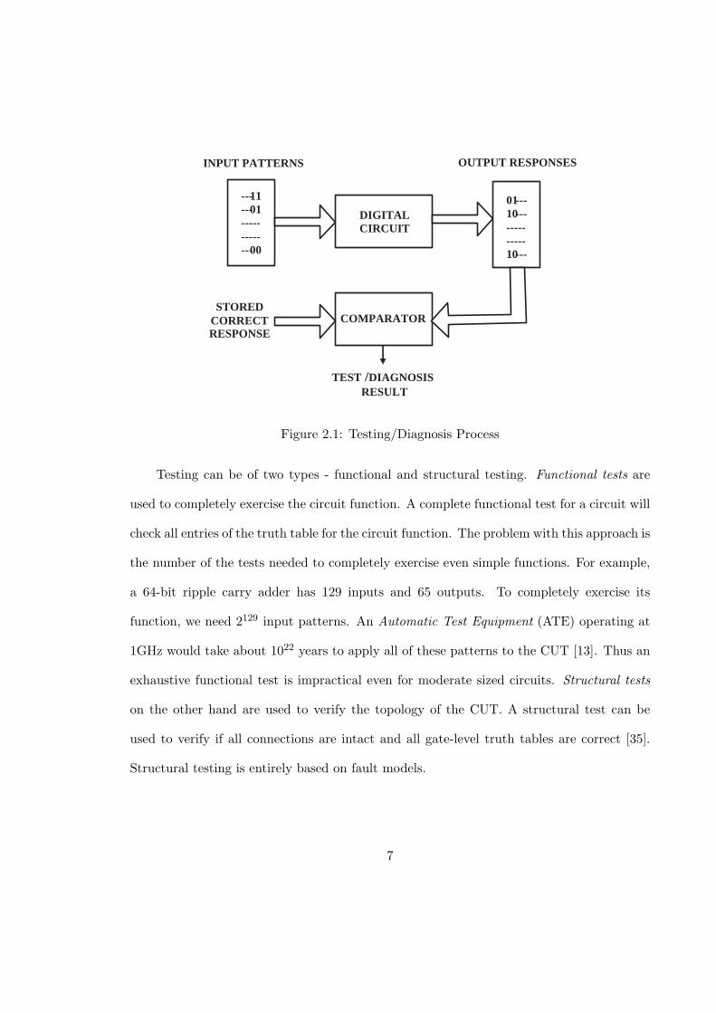
2.2 Testing/Diagnosis Process

The basic process of testing or diagnosing a digital circuit is shown in Figure 2.1 [13].

During testing the digital circuit is referred to as Circuit under Test (CUT), and during

diagnosis it is referred as Circuit under Diagnosis (CUD). Binary test vectors are applied

to the CUT/CUD. The response of the CUT/CUD to a test vector is compared with the

stored correct response. A mismatch between the stored and observed responses indicates

a bad circuit.

The input data to the CUT/CUD is referred to as the test pattern or test vector. A

collection of test vectors designed to exercise whole or part of the circuit is called a test

set. There are two kinds of tests: fault detection tests and fault diagnostic tests [16]. Fault

detection tests are used for the purpose of testing and they tell us whether the CUT is

faulty or fault-free. They do not give any information on the identity (type, location) of

the fault. A diagnostic test is applied after a circuit has failed the testing process. Its aim

is to identify the fault that caused the circuit to fail.

2.3 Testing

Testing is the process of verifying if the manufactured chip has the intended functional-

ity and timing. The test inputs to a digital IC (Integrated Circuit) are developed to exercise

the implemented function or to detect modeled faults [6].

6

STORED CORRECT RESPONSE

COMPARATOR

DIGITAL CIRCUIT

--- 11 --- 01 ----- ----- --- 00

01 --- 10 --- ----- ----- 10 ---

TEST / DIAGNOSIS RESULT

INPUT PATTERNS OUTPUT RESPONSES

Figure 2.1: Testing/Diagnosis Process

Testing can be of two types - functional and structural testing. Functional tests are

used to completely exercise the circuit function. A complete functional test for a circuit will

check all entries of the truth table for the circuit function. The problem with this approach is

the number of the tests needed to completely exercise even simple functions. For example,

a 64-bit ripple carry adder has 129 inputs and 65 outputs. To completely exercise its

function, we need 2129 input patterns. An Automatic Test Equipment (ATE) operating at

1GHz would take about 1022 years to apply all of these patterns to the CUT [13]. Thus an

exhaustive functional test is impractical even for moderate sized circuits. Structural tests

on the other hand are used to verify the topology of the CUT. A structural test can be

used to verify if all connections are intact and all gate-level truth tables are correct [35].

Structural testing is entirely based on fault models.

7

2.4 Fault Modeling

A defect is the unintended difference between implemented hardware and its intended

design [13]. Defects are those that could occur in a fabricated IC. A fabricated chip could

have many types of defects, for example, breaks in signal lines, lines shorted to ground,

lines shorted to VDD, etc. Fault modeling is the translation of real world defects to a

mathematical construct that can be operated upon algorithmically and understood by a

software simulator for the purpose of providing a metric for quality measurement [21].

Thus physical defects are modeled as faults because the analysis of faults is much simpler.

Also, fault models greatly simplify the test generation process. Physical defects can be

modeled as either logical faults or delay faults, depending on whether the defect affects the

logical behavior or the time of operation. Fault models can represent many, though not all

physical defects.

2.4.1 Single Stuck-at Fault Model

This is the earliest and most widely used fault model to date. Eldred’s 1959 paper [27]

laid the foundation for the stuck-at fault model, though that paper did not make any

mention of the stuck-at fault. The term “stuck-at fault” first appeared in the 1961 paper

by Galey, Norby and Roth [33].

Stuck-at faults are gate-level faults modeled by assigning a fixed ‘0’ or ‘1’ value to an

input or an output of a logic gate or a flipflop [13]. Each interconnection in a circuit can have

two faults, stuck-at-1 (sa1, s-a-1) and stuck-at-0 (sa0, s-a-0). If we assume that there can be

several simultaneous stuck-at faults, then in a circuit with n interconnections between gates

there are 3n − 1 possible multiple stuck-at faults. All combinations except the one having

8

all lines as fault-free are treated as faults. It is evident that even for moderate values of n,

the number of multiple stuck-at faults could be very large. Thus it is a common practice to

model only single stuck-at faults. Therefore the assumption is that only one stuck-at fault

is present in a circuit at a time. In a circuit with n interconnections there can be no more

than 2n single stuck-at faults. This number can be further reduced using fault collapsing

techniques [13, 69] discussed in Section 2.6. Numerous algorithms have been developed and

programmed to efficiently generate tests for single stuck-at faults [66, 36, 31, 65, 43, 71, 72].

2.4.2 Other Fault Models

Other than stuck-at faults there are bridging faults that model electrical shorts between

signal lines occurring at the wafer level. Then there are transition delay faults that model

gross delay defects (such as pinched metal lines, resistive contacts, etc.) at gate terminals.

Path delay faults model small distributed delay defects which cause timing failures in the

chip. The detection of transition and path delay fault requires a pair of vectors. The IDDQ

faults are those that elevate the steady state current in the circuit. For example, transistor

shorts can be effectively modeled as IDDQ faults. As can be seen each fault model, models

unique types of defects. Details of these fault models can be found in [13].

2.5 Relations among Faults

Consider two faults f1 and f2. Let T (f1) and T (f2) be the sets of all the test vectors

that detect f1 and f2 respectively. The following relations can be defined for a pair of

faults.

9

T( f1 )=T (f2) T( f2 )

T (f 1 )

T( f1 ) T( f1 ) T (f2) T (f2)

(a) f1 and f2 are equivalent (b ) f 2 dominates f 1

( c ) f1 and f2 are i ndependent ( d ) f1 and f2 are c oncurrent

Figure 2.2: Relations Between Faults f1 and f2

2.5.1 Fault Equivalence

Two faults are said to be equivalent, if and only if the corresponding faulty circuits

have identical output functions [13]. Equivalent faults cannot be distinguished by any test

vector, i.e., a test for one fault will also detect the other fault. Thus the two faults have

the exact same test sets as shown in Figure 2.2(a).

2.5.2 Fault Dominance

If all tests of fault f1 detect another fault f2, then f2 is said to dominate f1. This

relation is shown in Figure 2.2(b), where T (f1) ⊆ T (f2). Thus any test for the dominated

fault (f1) will also be a test for the dominating fault (f2). Notice that fault equivalence

10

is a special condition of fault dominance in which two faults dominate each other. So,

dominance is a more basic relation than equivalence.

2.5.3 Fault Independence

Two faults are said to be independent if and only if they cannot be detected by the

same test vector [7, 8], i.e., they have no common test. Thus, if f1 and f2 are independent

then T (f1) and T (f2) are disjoint sets as shown in Figure 2.2(c).

2.5.4 Fault Concurrence

Two faults that neither have a dominance relationship nor are independent are defined

as concurrently-testable faults [24]. The concurrently-testable faults can have two types of

tests as depicted in Figure 2.2(d):

1. Each fault has an exclusive test that does not detect the other fault [3].

2. A common test called the concurrent test in [24], that detects both faults.

Concurrently-testable faults have also been referred to as compatible faults in the litera-

ture [7].

2.6 Fault Collapsing

We had seen that for a circuit with n interconnections we would have 2n stuck-at faults.

Clearly this number would become very large for big circuits, and would result in longer

test set generation times. Fault Collapsing is the process of reducing the number of faults

that need to be targeted for test generation, without any penalty on the fault coverage. It

11

is done by utilizing the relations defined in the previous section. The relative size of the

collapsed set with respect to the set of all faults is called the collapse ratio [13]:

Collapse ratio =|Set of collapsed faults|

|Set of all faults|

Fault collapsing can be classified into two types, Equivalence collapsing and Dominance

Collapsing. Equivalent fault collapsing involves partitioning all faults into disjoint equiv-

alent fault sets such that all faults in a set are equivalent to each other, and selecting

one representative fault from each set. The resulting set of faults is called an equivalence

collapsed fault set. A test vector which detects the representative fault of an equivalent

fault set will also detect all other faults belonging to that set. So we need to generate a

test only for the representative fault. This reduces the test generation time. It should be

noted that equivalence collapsing does not affect the diagnostic resolution, i.e., the ability

to distinguish between faults.

In the case of large circuits, where coverage (detection) of faults is more important

than their exact location (diagnosis), dominance fault collapsing may be desirable [23]. For

a pair of faults having a dominance relation, a test for the dominated fault will also detect

the dominating fault. Thus the dominating fault can be dropped from the target fault

list. However there is a drawback to dominance fault collapsing. In case the dominated

fault is redundant, i.e., it does not modify the input-output function of the circuit and

cannot be detected by any test, there would be no test for the dominating fault even if it

is detectable. Dominance collapsing always results in a smaller set than the equivalence

collapsed set. Though dominance collapsing produces a smaller collapsed fault set, the

12

tests for the collapsed faults may not guarantee 100% fault coverage. Hence equivalence

collapsing is more popular.

For example, consider an n-input AND gate. The total number of stuck-at faults is

2n + 2. All single s-a-0 faults on the inputs and output of the AND gate are equivalent.

Thus, using equivalence collapsing, the number of stuck-at faults is reduced to n + 2. Also,

the output s-a-1 fault dominates a single s-a-1 fault on any input and hence the output s-

a-1 can be left out of the target fault set. Thus, dominance fault collapsing further reduces

the number of faults for an n-input AND gate to n + 1. Similar results for dominance and

equivalence fault collapsing can be derived for other Boolean gates as well. It must be noted

that faults on a fanout stem and branches cannot be collapsed.

Equivalence and dominance fault collapsing can either be performed at a functional or

structural level. Functional collapsing is based on the effect of faults on the Boolean function

of the circuit [4]. For an n-line circuit there are 2n single stuck-at faults, and the Boolean

equation has to be applied to 2n2−1 pairs of faults to determine all equivalence/dominance

relations [13]. Also, it will be cumbersome to manipulate large Boolean functions. For these

reasons structural collapsing is used in practice. In structural collapsing relations between

faults are determined for simple Boolean gates and are then applied to larger circuits.

The size of the fault set can be further reduced by performing hierarchical fault collaps-

ing as described in [4, 5, 63, 68, 70]. Most definitions for fault equivalence and dominance,

appearing in the literature, correspond to single output circuits. For such circuits, fault

equivalence defined on the basis of indistinguishability (identical faulty functions) implies

that the equivalent faults have identical tests. However, for multiple output circuits, two

faults that have identical tests can be distinguishable if their output responses are not the

13

same. This leads to diagnostic equivalence and diagnostic dominance which are extended

definitions for equivalence and dominance respectively [68, 70].

2.7 Fault Simulation

Fault simulation is the process of computing the response of a faulty circuit to given

input stimuli. The program that performs fault simulation is called a fault simulator. The

basic operation of a fault simulator is as follows: Given a circuit, a test input and a fault,

the fault simulator inserts the fault into the circuit and computes its output response for

the test input. It also computes the good circuit response to the same test input. Finally it

declares the fault as detected if there is mismatch between the good and faulty responses.

Thus for a test set and a fault list the fault simulator can give the fault coverage of the test

set. Fault coverage is defined as [13],

Fault Coverage =Number of faults detected

Number of faults in initial fault list

Notice that the fault simulator can determine which faults are detected by which test

vectors. We have used this feature of the fault simulator extensively in our work. Also, a

fault simulator is used along with an Automatic Test Pattern Generator (ATPG) for test

generation.

There are several algorithms for fault simulation, the simplest being the serial fault

simulation. Here fault simulation is performed for one fault at a time. As soon as one fault

is detected, the simulation is stopped and a new simulation is started for another fault.

This fault simulation method, though simple, is very time consuming.

14

Another technique of fault simulation, which simulates more than one fault in one pass

is called parallel fault simulation. It makes use of the bit-parallelism of logical operations

in a digital computer [13]. The parallel fault simulator can simulate a maximum of w − 1

faults in one pass, where w is the machine word size. So, a parallel fault simulator may run

w − 1 times faster than a serial fault simulator. Other fault simulation algorithms include

Test-Detect [67], Deductive [9], Concurrent [77, 78], Differential [18], etc.

2.8 Test Generation

Automatic test pattern generation is the process of generating input patterns to test a

circuit, which is described strictly with a logic-level netlist [13]. These programs usually op-

erate with a fault generator program, which creates the collapsed fault list. Test generation

approaches can be classified into three categories: exhaustive, random and deterministic.

In the exhaustive approach, for an n-input circuit, 2n input patterns are generated.

The exhaustive test set guarantees 100% fault coverage (ignoring the redundant faults if

any). It is evident that this approach is feasible only for circuits with very small number of

primary inputs.

Random test generation is a simple approach in which the input patterns are generated

randomly. Fault simulation is performed for every randomly generated pattern. A pattern

is selected only if it detects new faults. In a typical test generation process, random patterns

are used for achieving an initial 60-80% fault coverage, after which deterministic test pattern

generation can be employed to achieve the remaining coverage [2].

Deterministic Automatic Test Pattern Generator (D-ATPG) algorithms are based on

injecting a fault into a circuit, and determining values for the primary inputs of the circuit

15

that would activate that fault and propagate its effect to the circuit output. In deter-

ministic test generation, the search for a solution involves a decision process for selecting

an input vector from the set of partial solutions using an algorithmic procedure known as

backtracking. In backtracking, all previously assigned signal values are recorded, so that

the search process is able to avoid those signal assignments that are inconsistent with the

test requirement. The exhaustive nature of the search causes the worst-case complexity to

be exponential in the number of signals in the circuit [32, 42]. To minimize the total time,

a typical test generation program is allowed to do only a limited search in the number of

trials or backtracks, or the CPU time.

The most widely used deterministic automatic test pattern generation algorithms are:

D-algorithm [66], PODEM (Path-Oriented Decision Making) [36] and FAN (Fanout-Oriented

Test Generator) [31]. The faults left undetected after the D-ATPG phase are either redun-

dant faults for which no test exists, or aborted faults that could not be detected due to

CPU time limit.

2.9 Failure Analysis

Testing of fabricated chips prevents the shipment of defective parts, but improving

the production quality of the chips depends on effective failure analysis. A better quality

production process means higher yield, i.e., more usable die. Typically, an IC product

goes through two manufacturing stages [52]: (1) prototype stage, and (2) high-volume

manufacturing stage.

During the prototype stage, a small number of sample chips are produced to verify

the functionality and timing of the design. The chips may fail badly due to design bugs or

16

manufacturing imperfections. All issues that cause the chip to fail must be addressed so

that these do not recur when the design goes into mass production. It is here that failure

analysis comes into play.

After the prototype stage, the product is ready for high-volume production. In this

stage there could be fluctuations in the yield mainly due to manufacturing errors. Contin-

uous yield monitoring is necessary from time to time to respond to unexpected low-yield

situations [50]. Here again failure analysis is the means for yield improvement.

Some of the methods of failure analysis consist of etching away certain layers, imag-

ing the silicon surface by scanning electron microscopy (SEM) or focused ion beam (FIB)

systems, particle beams, etc. [52]. Any analysis performed directly on the defective chip is

called physical analysis. With millions of transistors and several layers of metals, physical

analysis process is often laborious and time consuming. Thus physical inspection of the chip

is not feasible without an initial suspect list of defect sites. It is the job of fault diagnosis

to guide the physical analysis process by providing the suspected defect locations.

2.10 Fault Diagnosis

Fault diagnosis is the first step in failure analysis which by logical analysis gives a list

of likely defect sites or regions. Basically, fault diagnosis narrows down the area of the chip

on which physical examination needs to be done to locate defects. Fault diagnosis involves

applying tests to failed chips and analyzing the test results to determine the nature of the

fault. A test set used for the purpose of diagnosis is referred to as a diagnostic test set [16].

The test sets are constructed so as to ideally pin-point to a single fault candidate. Such a

characteristic of a diagnostic test set is called its diagnostic resolution. The highest number

17

of fault candidates reported for a test in the diagnostic test set is referred to as its diagnostic

resolution. Precision of fault diagnosis is very critical as it leads to physical analysis. If a

wrong site or location is predicted then the actual defect site could be damaged during the

physical inspection process of the predicted site.

2.11 Linear Programming

In the work described in this thesis, the optimization of detection and diagnostic test

sets is done using linear programming techniques. Thus, the current and the subsequent

sections of this chapter give a brief review of linear programming.

Linear Programming (LP) is the method of selecting the best solutions from the avail-

able solutions to a problem. It is the most widely used method of constrained optimization

in economics and engineering fields.

The main elements of any linear program are,

1. Variables: The goal is to find the values for the variables that provide the best value

of the objective function. These values are unknown at the start of the problem.

LP assumes that all variables are real valued, meaning that they can take fractional

values.

2. Objective function: This is a linear mathematical expression that uses the variables

to express the goal of optimization. The goal of the LP problem is to either maximize

or minimize the value of the objective function.

3. Functional Constraints: These are linear mathematical expressions that use the

variables to express certain conditions that need to be met while looking for the

possible optimum solution

18

4. Variable Constraints: Usually variables have bounds. Very rarely are the variables

unconstrained.

With the advancements in computing power and algorithms for solving LPs, the largest

optimization problems today could have millions of variables and hundreds of thousands of

constraints. These large problems can be solved in practical amounts of time.

2.11.1 Standard LP Problems

LP problems can have objective functions to be maximized or minimized, constraints

may be inequalities (≤, ≥) or equalities (=), and variables can have upper or lower bounds.

There are two standard classes of problems - the standard maximum problem and the stan-

dard minimum problem [28]. In these problems all variables are constrained to be non-

negative, and all functional constraints are inequalities. These two play an important role

because any LP problem can be converted to one of these two standard forms.

We are given an m-vector, b = (b1, . . ., bm)T , an n-vector, c = (c1, . . ., cn)T , and an

m × n matrix of real numbers,

A =

a11 a12 . . . a1n

a21 a22 . . . a2n

. . . .

. . . .

am1 am2 . . . amn

The Standard Maximum Problem [28] is to find an n-vector, x = (x1, . . ., xn)T ,

to Maximize

P = c1x1 + c2x2 + ... + cnxn (or P = cT x)

19

subject to the constraints,

a11x1 + a12x2 + . . . + a1nxn ≤ b1

a21x1 + a22x2 + . . . + a2nxn ≤ b2

. (or Ax ≤ b)

.

am1x1 + am2x2 + . . . + amnxn ≤ bm

and

x1 ≥ 0, x2 ≥ 0, . . . , xn ≥ 0 (or x ≥ 0)

Here, xj and cj (where j = 1, 2, ..., n) are the variables and coefficients respectively in

the objective function. P is the objective function value that needs to be maximized. bi are

the limits, and aij (where i = 1, 2, ..., m) are the coefficients of the functional constraint

equations.

Similarly the Standard Minimum Problem [28] is to find an m-vector, y = (y1, . . ., yn)T ,

to Minimize

Q = b1y1 + b2y2 + ... + bmym (or Q = yT b)

subject to the constraints,

a11y1 + a12y2 + . . . + am1yn ≥ c1

a12y1 + a22y2 + . . . + am2yn ≥ c2

. (or yT A ≥ cT )

.

a1ny1 + a2ny2 + . . . + amnyn ≥ cn

20

and

y1 ≥ 0, y2 ≥ 0, . . . , ym ≥ 0 (or y ≥ 0)

Here, yi and bi (where i = 1, 2, ..., m) are the variables and coefficients respectively in

the objective function. Q is the objective function value that needs to be minimized. cj are

the limits, and aij (where j = 1, 2, ..., n) are the coefficients of the functional constraint

equations.

Many algorithms have been proposed to solve linear programs. One of the oldest and

most popular methods is the simplex method [10, 22] invented by George Dantzig in 1947.

It is a robust method as it can solve any linear program. Interior-point method found by

Karmarkar [49] is a polynomial time method and is preferred over the simplex method for

extremely large problems.

2.12 Primal and Dual Problems

If we have an optimization problem defined for an application, we could define another

optimization problem called the dual problem. The original problem now will be called the

primal problem. These two problems share a common set of coefficients and constants. If

the primal minimizes one objective function of one set of variables then its dual maximizes

another objective function of the other set of variables

Let us look at the duality for the standard problems defined previously. As in Sec-

tion 2.11.1, c and x are n-vectors, b and y are m-vectors, and A is an m × n matrix. We

assume m ≥ 1 and n ≥ 1.

The dual of the standard maximum problem is the standard minimum problem. The

definitions of the primal maximum problem and the dual minimum problem are given in

21

Table 2.1: Primal and Dual Problem Definition

Standard Maximum Standard MinimumProblem (Primal) Problem (Dual)

Maximize P = cT x Minimize Q = yT bsubject to, subject to,

Ax ≤ b yT A ≥ cT

and x ≥ 0 and y ≥ 0

Table 2.1. Another way to look at this is the dual of the standard minimum problem is the

standard maximum problem. Hence the two problems are called duals.

The primal and dual LP problems are related by an important property called dual-

ity. This property indicates that we may in fact solve the dual problem in place of or in

conjunction with the primal problem.

Duality theorem states that if the primal problem has an optimal solution, then the

dual also has an optimal solution, and the optimized values of the two objective functions

are equal [75].

There is a twofold advantage in studying the dual problem. First, its implementation

enhances the understanding of the original (primal) model. Second, it is sometimes com-

putationally easier to solve the dual model than the original model, and likewise provides

the optimal solution to the latter at no extra cost.

2.13 Integer Linear Programming (ILP)

ILP is a variant of LP where the variables can take on only integer values. In ILP

the number of solutions grows extremely rapidly as the number of variables in the problem

increases. This is because of the numerous possible ways of combining these variables. Thus

the worst case computational complexity of ILP problems is exponential.

22

Special algorithms such as branch and bound method [10] have been developed to find

optimal integer solutions. However, the size of problem that can be solved successfully by

these algorithms is an order of magnitude smaller than the size of linear programs that can

easily be solved. The LP problem has polynomial complexity due to its continuous decision

space, as the variables can take fractional values. Thus in some cases the ILP problem is

converted to a relaxed-LP problem by allowing the variables to take on real values, after

which rounding algorithms are used to obtain an integer solution.

The primal-dual problems of LP described in the previous section can be transformed

into two ILP problems by treating the variables as integers. The ILP problems share several

of the duality properties.

2.14 Applications of Linear Programming in Testing

The ILP techniques have been used to optimize various aspects of testing. They have

been used to obtain optimization of test sets for both combinational [29] and sequential

circuits [26] as well as for globally minimizing N-detect tests [47, 46] and multiple fault model

tests [81]. Other applications for the ILP techniques include test resource optimization [14,

58] and test data compression [15] for the testing of SoCs.

As stated earlier the computational complexity of the ILP would be too high to obtain

an optimum solution for even medium size circuits. For this reason reduced-complexity LP

variations such as the recursive rounding technique [48] can be used. The recursive rounding

technique has been described in detail in the appendix.

23

Chapter 3

Previous Work on Detection Test Set Minimization

This chapter gives a background of the various compaction techniques that have been

proposed for detection test set minimization. In this chapter test set minimization/compaction

is in the context of detection test sets only.

Before discussing the various test minimization techniques described in the literature let

us look at the concept of independent fault set (IFS), which plays an important role in test

minimization.

3.1 Independent Fault Set

In Section 2.5 we had seen the definition of the independence relation between a pair of

faults. Two faults are called independent if no vector can detect both [7]. An independent

fault set (IFS) contains faults that are pair-wise independent. Thus we need one vector for

every fault in the IFS. Hence the cardinality of the largest IFS for a circuit provides a lower

bound on the size of a complete fault detection test set [7].

3.2 Independence Graph

The independence relations among faults can be represented graphically as an inde-

pendence graph (also known as incompatibility graph). In an independence graph the nodes

represent faults, and the edges between nodes represent the pair-wise independence rela-

tions between faults. As independence is a symmetric relation the edge does not require a

24

direction. Thus an edge between two nodes means that the two corresponding faults cannot

be detected by a common vector. And the absence of an edge between two nodes indicates

that the corresponding two faults can be detected by a common test vector, i.e., the two

faults could have equivalence, dominance or concurrence relation.

Figure 3.2 shows the independence graph for ISCAS85 [40] benchmark circuit c17 [23].

The circuit has 17 nets, so there will be 34 single stuck-at faults. Using functional dominance

collapsing of [69] the number of faults is reduced to eleven. Figure 3.1 shows the eleven faults

in the c17 circuit, numbered 1 through 11. The edges in the independence graph represent

functional independences and were found using the ATPG-based procedure described in [23].

Here it should noted that if the independence graph is for a dominance collapsed fault set,

then the absence of an edge between two nodes means that the two faults are concurrently-

testable.

x

x x

x

x

x

4 x

x

x

2

x

x 1

6

8

7 3

5

9

1 0

11

Faults numbered 1 through 11 are all s - a - 1 t yp es

Figure 3.1: c17 Circuit with 11 Functional Dominance Collapsed Faults [69]

In an independence graph the nodes belonging to a clique form an IFS. A clique is a

subgraph in which every node is connected to every other node [20]. A maximum clique is

25

2 3 4 5

6 7 8 9 10

11

1

Figure 3.2: Independence Graph for c17 Benchmark Circuit

a clique of largest size i.e., with the highest number of nodes. Thus the maximum clique of

an independence graph will give the largest IFS.

From the independence graph of c17, redrawn in Figure 3.3, it is clear that nodes

(faults) 1, 2, 4 and 5 form an independent fault set (IFS). So, in order to detect all faults

in c17, we need at least 4 vectors. Actually, the minimum possible test set for c17 has

four vectors. In general, however, the size of largest IFS is only a theoretical minimum and

such a test set whose size equals the lower bound may not be achieved in practice for many

circuits. This was shown in [46] where, for a 5-bit and 6-bit multiplier a minimum test set

of 7 test vectors was obtained, whereas the theoretical lower bound for these multipliers is

6.

One important point to make note of is that a circuit can have multiple maximal

independent fault sets. For example, Figure 3.4 shows the same independence graph for c17

26

2 3 4 5

6 7 8 9 10

11

1

Figure 3.3: Largest Clique in the Independence Graph of Figure 3.2

with another maximum clique formed by nodes numbered 6, 7, 8 and 9. The four faults

corresponding to these nodes also form a maximal IFS.

3.3 Need for Test Minimization

Compact test sets are very important for reducing the cost of testing VLSI circuits by

reducing test application time and test storage requirements of the tester. This is especially

important for scan-based circuits as the test application time for such circuits is directly

proportional to the test set size and number of flip-flops used in the scan chain.

3.4 Test Set Compaction

The test minimization problem for combinational circuits has been proven to be NP-

complete [51, 34]. Most ATPGs are not concerned with generating minimal test sets, as test

27

2 3 4 5

6 7 8 9 10

11

1

Figure 3.4: Multiple Maximum Cliques in the Independence Graph of Figure 3.2

generation is in itself computationally difficult. Thus ATPGs adopt a localized approach

by targeting a single fault and generating a test vector for that fault. So heuristic methods

based on compaction algorithms are used to obtain a minimal test set.

There are two types of compaction techniques - static compaction and dynamic com-

paction.

3.4.1 Static Compaction

Static compaction, also known as post-generation compaction [17], techniques are used

to compact a given test set. Static compaction techniques work only with already generated

test vectors. Hence these techniques are usually independent of the test generation process.

Several static compaction algorithms based on different heuristics exist in the literature and

are discussed next.

28

One of the most popular static compaction techniques is reverse order fault simula-

tion [72], where the generated test vectors are simulated in the reverse order, hoping to

eliminate some of the initially generated vectors. This method is very effective because the

normal test generation often starts with a random phase, where random vectors are simu-

lated until no new faults are being detected and then a deterministic ATPG phase begins,

where fault-specific vectors are generated. This is done so that the test pattern generation

effort is not wasted on the easy to detect faults that can be detected by random vectors. The

random vector generation phase is one of the main sources of redundant test vectors. Fault

simulation of the test vectors in the reverse order removes most of the initially generated

random vectors, which are made redundant by the deterministic vectors.

Another static compaction technique is described by Goel and Rosales [37], where

pairs of compatible test vectors, that do not conflict in their specified (0, 1) values, are

repeatedly merged into single vectors. This method is suitable only for patterns in which

the unassigned inputs are left as don’t care (X) by the ATPG program. Also, the compacted

test set will vary depending on the order in which vectors are compacted. One drawback of

this technique is that little reduction in test set size can be achieved for a highly incompatible

test set.

The paper [45] describes a test ordering technique called double detection which com-

bines static and dynamic compaction. In this technique, during test generation a fault is

not dropped from the fault list until it is detected twice. Each vector is assigned a variable

to keep a count of the number of faults it uniquely detects. At the end of the test generation

if a vector has a count 0 it means that all the faults detected by it are also detected by

29

other vectors. But this does not mean that the vector is redundant, because it may be-

come an essential vector for a fault on eliminating some other vector after fault simulation.

Fault simulation is performed during which all vectors with non-zero counts are simulated

first, followed by the vectors with zero counts in the reverse order. This time many vectors

with 0 counts become redundant, i.e., those that do not detect any new fault, and can be

eliminated.

In all of the techniques described above, the size of the compacted test set depends on

the order in which the vectors are compacted. One static compaction technique in which

the order of vectors does not influence the final compacted test set size is the integer linear

programming (ILP) method called the Test Minimization ILP [29]. The test minimization

ILP gives the most compact test set possible for the given test set. However, it should be

noted that the complexity of the ILP is exponential. Other linear programming (LP) based

techniques like recursive rounding [48] that have polynomial time complexity can be used

to obtain a close to optimum test set. The work presented in this thesis makes extensive

use of the test minimization ILP along with recursive rounding. The test minimization ILP

is described in the next chapter and the details of the recursive rounding technique can be

found in Appendix A.

One of the main advantages of static compaction is that no modification of the ATPG is

needed, as it is independent of the test generation process. Though static compaction adds

to the test generation time, this time is usually small compared to the total test generation

time. However optimal static compaction algorithms are impractical, so heuristic algorithms

are used. Static compaction can also be used after dynamic compaction to further compact

the test sets.

30

3.4.2 Dynamic Compaction

In the literature techniques that attempt to reduce the number of test vectors during

test generation have been classified as dynamic compaction techniques. There are some

other techniques in literature classified as static which work after test generation and signif-

icantly modify or replace previously generated vectors based on the fault simulation infor-

mation. We have classified such techniques as dynamic. Thus there are two sub categories

of dynamic compaction.

Dynamic Compaction during Test Generation

Dynamic compaction techniques under this category attempt to reduce the number of

test vectors while they are being generated. These techniques require modifications in the

test generation process and algorithms. The key idea of compaction during test generation

is that if the fault coverage of each test pattern is maximized during test generation, then

the total number of patterns can be reduced.

The first dynamic compaction procedure was proposed by Goel and Rosales [37] in

which every partially specified test vector is processed immediately after its generation

by trying to use only the unspecified inputs in the test vector to derive a test to detect

additional faults by the same vector.

Akers and Krishnamurthy were the first to present test generation and compaction

techniques based on independent faults [7]. As the minimum test set size cannot be smaller

than the size of the largest independent fault set (IFS), the tests for independent faults

can be considered necessary. For every fault in a maximal IFS, partially specified tests are

found using the test value propagation technique. Each partially specified test also gives

31

information on which other faults can be potentially detected by it. This process is repeated

for a different maximal IFS. While each pair of faults within an IFS requires separate tests,

there is a definite possibility that a pair of faults from different IFSs can be detected by a

single test. Thus a fault matching procedure was used to find sets of compatible faults, i.e.,

faults that can be detected by a single test vector, from the independent fault sets. The

authors suggested that the information on compatible fault sets and independent fault sets

could be used to decide the order of faults to be targeted during test generation. Thus these

techniques could be used as a pre-processing step to the test generation step. However they

did not provide any specific technique for fault ordering. Results for benchmark circuits are

also not given. Though this paper did not provide any results, it became the basis for later

work on independent faults.

COMPACTEST [59] was the first technique to make use of independent faults for fault

ordering. The target faults are ordered such that the faults present in largest maximum

independent fault sets (MIFS) appear at the beginning of the fault list. Later Kajihara

et al. [45] proposed dynamic fault ordering which is an enhancement of the fault ordering

technique of COMPACTEST. Here the fault list is reordered whenever a test is generated.

The independent fault set with largest number of undetected faults at that point is put at

the beginning of the fault list.

The “double detection algorithm” [45] described earlier in the section on static com-

paction is also a dynamic compaction technique. Here the processing done during test

generation falls under the dynamic compaction category.

A redundant vector elimination (RVE) algorithm, which identifies redundant vectors

during test generation and dynamically drops them from the test set, was developed by

32

Hamzaoglu and Patel [38]. The RVE algorithm fault simulates all the faults in the fault list

except the ones that are proven to be untestable, and it keeps track of the faults detected

by each vector, the number of essential faults of each vector and the number of times a fault

is detected. The essential faults of a vector are those that cannot be detected by any other

vector in the vector set [17, 45]. During test generation if the number of essential faults of

a vector reduces to zero, i.e. the vector becomes redundant, and it is dropped from the test

set. The compaction results of RVE algorithm were similar to those of the double detection

algorithm of [45].

Another recent work on dynamic compaction involves independence fault collapsing [25,

23] and concurrent test generation [24, 23], which collapses faults into groups based on

independence relation, and then for each group tries to generate either a single vector, or

as few vectors as possible, which can detect all faults in that group. In the independence

fault collapsing algorithm an independence graph is constructed for a dominance collapsed

fault set. In such a graph the absence of an edge between two nodes indicates that the

corresponding two faults are concurrently testable. Thus two nodes that are not connected

by an independence edge can form a single node whose label combines the fault labels of both

nodes. Then, all nodes that had edges connecting to the two nodes will have edges to the

combined node. This collapsing procedure ends when the graph becomes fully-connected.

However, depending on the order in which the nodes are collapsed the size of the collapsed

graph can vary. Thus the collapsing of faults in the independence graph is done using

metrics - degree of independence defined for every fault and similarity metric defined for

every pair of faults. This algorithm groups faults into nodes such that the similarity metrics

among faults within each group are minimized. This increases the possibility of finding a

33

single concurrent test for the group. Concurrent test generation technique is used to find

a single or as few test vectors as possible to detect all faults in each group. However these

two techniques were very computationally intensive and could not provide optimum results.

Dynamic Compaction after Test Generation

Compaction methods under this category are mainly based on essential fault pruning,

and have been classified in the literature as static techniques as they are applied after the

test generation process. But, we will consider them as dynamic techniques as the test

vectors are modified or even replaced by new vectors during the compaction process. The

main advantage of the dynamic compaction techniques in this category is that the level of

compaction achievable is not dependent on the quality of the original test set, as opposed

to static compaction.

Chang and Lin [17] proposed the forced pair-merging algorithm which involves mod-

ification of one vector to cover the essential faults of another vector. The essential faults

of a vector are those that cannot be detected by any other vector in the vector set. For

a vector say t1, as many specified (0s and 1s) bits as possible are replaced with Xs such

that the vector still detects its essential faults. Then, for each of the remaining vectors,

say t2, the algorithm tries to change the bits that are incompatible with the new t1 to Xs.

If the process succeeds, the pair is merged into a single vector. The authors also propose

essential fault pruning (EFP) method to achieve further compaction by removing a vector

by modifying other vectors of the test set to detect all the essential faults of the target

vector. A limitation of this method is its narrow view of the problem; it is not possible to

remove all the essential faults of a vector.

34

Kajihara, et al. give the essential fault extraction (EFE) algorithm in [44]. The EFE

is similar to EFP, wherein instead of modifying existing vectors, new vectors are generated

by targeting essential faults. The authors also propose the Two-by-one algorithm in which

addition of a new test vector removes two other vectors in a given test set. After determin-

imng two tests to be removed the essential faults of these vectors are used as target faults

for the vector to be added.

In [39] the essential fault reduction (EFR) algorithm [39] is proposed which is an im-

proved version of the EFP method of [17]. EFR uses a multiple target test generation

(MTTG) procedure [17, 45] to generate a test vector that will detect a given set of faults.

The EFR algorithm makes use of the independence (incompatibility) graph to decide which

faults in a vector can be pruned through detection by another vector. The EFR algorithm,

redundant vector elimination (RVE) algorithm described in the previous sub-section, along

with dynamic compaction [37] and a heuristic for estimating the lower bound are incor-

porated into an advanced ATPG system for combinational circuits, and is called MinTest.

MinTest produced some of the smallest reported single-detect test sets for the ISCAS85 [12]

and ISCAS89 [11] (scan versions) benchmark circuits. However this technique was compu-

tationally expensive.

3.5 Methods of Finding Maximal IFS

The importance of independent fault sets (IFS) in the reduction of test set size has

been established in the previous sections. We also saw that the largest IFS provides a lower

bound on the test set size. This lower bound can be closely achieved by selecting tests from

the test vectors derived for the faults in the IFS [7, 8]. However, the problem of finding the

35

largest IFS is complex, and heuristics have to be used to find a maximal independent fault

set.

Akers and Krishnamurthy [7] were the first to describe the derivation of maximal IFS

from a set of faults within a given circuit by combining the notions of fault dominance and

fault independence. For a given circuit their procedure involved finding dominance and

independence relations among faults for primitive gates forming the circuit. Then use the

transitive property of fault dominance to find additional dominance relations among faults

in the entire circuit. The transitive property of fault dominance is, if a fault f1 dominates

f2 and f2 in turn dominates f3, then f1 dominates f3. They then create a graph with

undirected edges between nodes representing the independence relations between faults of

the primitive gates of the circuit. The authors give a theorem stating that if fault f1

dominates f2, f3 dominates f4, and f1 and f3 are independent then f2 and f4 are also

independent. Using this theorem, additional edges are added to the graph. In the final graph

a maximal clique gives the maximal IFS. It was here that the notion of an independent fault

graph was first introduced, though the term “independence fault graph” was not used.

In the paper by Tromp [76] a maximal independent fault set was found using a graph,

constructed based on necessary assignments [64] of all faults. Necessary assignments are

line values that must be set for a fault to be detected. There is an edge between two nodes

in the graph, if the necessary assignments of the faults corresponding to the nodes have

conflicting values, implying the faults are independent. A maximal IFS was found as a

maximal clique in the graph. The main problem with this technique is that it has high

computational complexity, as all pairs of faults have to be considered, and then a maximal

clique problem has to be solved over all pairs of faults. The paper [60] gives an improved

36

technique to compute independent fault sets based on necessary assignments. It allows

construction of an IFS incrementally, thus resulting in reduced computational complexity.

In the paper on COMPACTEST [59], due to the complexity of computing independent

faults sets for the entire circuit, independent faults sets are computed only within maximal

fanout free regions using a labeling procedure. It also shows that the IFS for a fanout free

region is also the IFS for the complete circuit.

Kajihara, et al. [45] give an improved method to find the necessary assignments uti-

lizing static learning [31] and unique sensitization [31, 72]. The use of these techniques

increases the number of necessary assignments, thereby increasing the potential to compute

larger maximal IFS. Heuristics are used to store the necessary assignments efficiently and

to simplify the identification process for independence of two faults.

In [39] a minimum test set size (MTSS) estimation technique is given to find lower

bounds on test set sizes. As the size of maximal IFS gives the lower bound on the test set

size, it computes the maximal IFS by finding the maximal clique in the independence graph

initially only for essential faults and then enlarging this clique by considering other faults.

37

Chapter 4

Minimal Test Generation using Primal-dual ILP Algorithm

In the previous chapters we saw that the size of the largest IFS gives a lower bound

on the test set size. This lower bound can be closely achieved by selecting tests from the

test vectors derived for the faults in the IFS. This chapter describes the formulation of a

dual ILP whose solution gives the largest IFS. The dual ILP is obtained by treating the

test minimization ILP as the primal problem. The latter part of this chapter gives the

primal-dual ILP based algorithm for generating a minimal detection test set, followed by

the results of the algorithm.

4.1 Test Minimization ILP

The Test Minimization ILP [29] falls under the category of static compaction as ex-

plained in Section 3.4.1. It is an exact solution to the problem of creating a minimum

detection test set. The level of compaction achievable by this method is conditional to the

original unoptimized test set. Thus, an absolute minimum test set for a circuit would be

given by the test minimization ILP solution if we start with the exhaustive vector set for

that circuit.

Suppose a combinational circuit has K faults. We are given a vector set V of J vectors

and we assign a [0, 1] integer variable vj , j = 1, 2, . . . , J to each vector. Without loss

of generality, we assume that all K faults are detected by these vectors. Our problem then

is to find the smallest subset of these vectors that detects all faults. The variables vj have

the following meaning:

38

• If vj = 1, then vector j is included in the selected vector set.

• If vj = 0, then vector j is discarded.

Fault Vector number (j)number (k) 1 2 3 4 . . . . . J

1 0 1 1 0 . . . . . 12 0 0 1 0 . . . . . 13 1 0 0 1 . . . . . 04 0 1 0 0 . . . . . 0. . . . . . . . . . .. . . . . . . . . . .K 1 1 0 0 . . . . . 1

Figure 4.1: Detection Matrix akj .

We simulate the fault set and the vector set without dropping faults. The result is

represented as a detection table (matrix) of 0s and 1s, shown in Figure 4.1. In this matrix,

an element akj = 1 only if fault k is detected by vector j.

The test minimization ILP problem is stated as,

MinimizeJ

∑

j=1

vj (4.1)

subject to,

J∑

j=1

vj akj ≥ 1; for k = 1, 2, ..., K (4.2)

39

vj ∈ integer[0, 1], j = 1, ..., J (4.3)

The constraint set given by equation (4.2) ensures that the kth fault is detected by

at least one vector in the selected vector set. The fact that we start with a vector set V

that detects all faults in the set F and the direction of inequality in constraints that allow

us to set any or all vj ’s to 1, guarantee the existence of a solution [26, 47]. Additionally,

the provable ability of the ILP to find the optimum, provided its execution is allowed to

complete, and the minimum requirement of 1 for every constraint guarantees the smallest

size test set.

4.2 Dual ILP

Treating the test minimization ILP problem described in the previous section as the

primal, we formulate another ILP called the dual ILP to obtain the largest IFS.

Suppose a combinational circuit has K faults. We are given a vector set V of J vectors.

Without loss of generality, we assume that all K faults are detected by these vectors. Recall

that in the test minimization ILP we had assigned a [0, 1] integer variable vj to vector j.

For the dual problem we assign a [0, 1] integer variable fk , k = 1, 2, . . . , K to each fault.

The dual ILP is stated as,

MaximizeK

∑

k=1

fk (4.4)

40

subject to,

K∑

k=1

fk akj ≤ 1; for j = 1, 2, ..., J (4.5)

fk ∈ integer[0, 1], k = 1, ..., K (4.6)

akj is the element of the detection matrix obtained by fault simualtion without fault

dropping as described in the previous section. Because a solution to the primal test min-

imization problem specified by equations (4.1), (4.2) and (4.3) exists, according to the

duality theorem [75], a solution of the dual fault set maximization problem given by equa-

tions (4.4), (4.5) and (4.6) must also exist. We interpret this solution as a fault set, which

contains fault k only if fk = 1. We show that the dual solution provides an independent

fault set.

Definition 1: We define a pair of faults that is detectable by a vector set V to be

conditionally independent with respect to a vector set V if no vector in the set detects both

faults.

In comparison, therefore, the conventional fault independence as defined in the litera-

ture [7, 8] would mean ”absolute” independence that is conditional to the exhaustive vector

set with an additional implication that the faults are irredundant. In a similar way, con-

ditional equivalence, conditional dominance, conditional compatibility or concurrence can

be defined with respect to a vector set. Each definition will then become “absolute”, as

41

defined in the literature [24, 25], when the vector set becomes exhaustive and the faults are

irredundant.

Definition 2: For a given vector set, a subset of all detectable faults in which no pair

of faults can be detected by the same vector, is called a conditionally independent fault set

(CIFS).

Theorem 1 A solution of the dual ILP of equations (4.4), (4.5) and (4.6) provides a largest

conditionally independent fault set (CIFS) with respect to the vector set V .

Proof: The jth constraint of the constraint set 4.5 consists of fault variables corre-

sponding to non-zero akj , i.e., faults detectable by jth vector. It allows only one of those

faults to be selected since no more than a single fk can be set to 1 in any inequality. Sup-

pose, we set fk = 1. Then, constraint inequalities of all other vectors that also detect the

kth fault will be violated if any other fault detectable by them was selected. Hence, setting

of fk = 1 ensures that no fault that is conditionally compatible with kth fault with respect

to vector set V can be selected. This guarantees that the selected set of faults will only

contain faults that are conditionally independent with respect to V .

The other part of theorem, i.e., the selected conditionally independent fault set is

largest, follows from the provable ability of ILP in finding the optimum solution if one exists.

Existence of a solution is guaranteed from the duality theorem [75], combined with the fact

that a solution of the primal test minimization problem exists. Note that the optimality

of the solution will lead to the largest fault set because the objective function 4.4 requires

maximization.

Theorem 2 For a combinational circuit, suppose V 1 and V 2 are two vector sets such

that V 1 ⊆ V 2 and V 1 detects all detectable faults of the circuit. If CIFS(V 1) and

42

CIFS(V 2) are the largest CIFS with respect to V 1 and V 2, respectively, then |CIFS(V 1)| ≥

|CIFS(V 2)|.

Proof: Let G1(U, E1) be the independence graph of the circuit under consideration,

where U is the vertex set and E1 the edge set. Each vertex in an independence graph

represents a fault, and the presence of an edge between any two vertices indicates that the

corresponding faults are independent. The independence relations among vertices in graph

G1 have been determined by the vector set V 1. Thus, CIFS(V 1) is a maximum clique in

the graph G1 and |CIFS(V 1)| is the clique number of G1. A maximum clique is a clique

of largest size and the clique number of a graph is defined as the number of vertices in a

maximum clique.

Consider a vector set V 2 such that V 1 ⊆ V 2. Let G2(U, E2) be the independence

graph relative to the vector set V 2. Thus, CIFS(V 2) is a maximum clique in G2, and

|CIFS(V 2)| is the clique number of G2. U is the vertex set and E2 is the edge set of G2.

The vectors in the set V 2 − V 1 can only invalidate the independence relations which

were determined by the vector set V 1, but cannot determine new independence relations

among the faults. Thus the edges in graph G1 either remain unchanged or some may be

deleted because of the vector set V 2, but no new edge can be added to graph G1.

Note that a graph may have several maximum cliques. As no new edge is added to

G1, the clique number cannot increase. If an edge is removed such that it was contained

in every maximum clique, its removal modifies all these cliques, decreasing their clique

numbers. Removing an edge from a clique of m vertices still leaves two cliques of m − 1

vertices each. If there is at least one maximum clique from which no edge is removed, then

that clique will remain unchanged and clique number will not decrease. Thus, removal

43

of an edge cannot increase the clique number and can only decrease it by 1. This is a

well-understood result in graph theory.

Theorem 2 implies that the largest CIFS should monotonically converge to the absolute

IFS as more vectors are added to an initial vector set. In addition, the augmented vector

set will contain multiple tests for each fault of the IFS. This would enhance the capability

of the primal ILP to select the “right” vector for each IFS fault such that all faults are

covered. Note that one vector per IFS fault is the best we can do.

4.3 A Primal-Dual ILP Algorithm

An absolute minimal test set would be given by the primal solution of Section 4.1 if

we start with the exhaustive vector set. For large number of primary inputs (PIs), that is

impractical. Even for a moderate number of PIs, the solution becomes costly because of the

exponential complexity of ILP [75]. In an alternative approach, we start with any vector

set and then find a conditionally independent fault set (CIFS) by solving the dual problem

stated in Section 4.2. In this process, we solve the dual ILP iteratively by generating

multiple-detect tests generated only for the CIFS. Once, the CIFS is sufficiently converged,

we solve the primal ILP to get a minimal vector set. This method belongs to the dynamic

test minimization category, where test generation and minimization are done interactively.

The primal-dual ILP algorithm for minimal detection test set generation consists of

the following steps:

1. Generate an initial vector set: We used the ATPG program ATALANTA [56] but

any other program can be used. In general, for combinational circuits close to 100%

coverage is obtained. In terms of the number of vectors, this set is non-optimal and

44

may contain many more vectors than the final minimized set. Some redundant faults

are identified and a few others are left undetected due to time or backtrack limits.

Both categories are removed from the fault set to obtain a target fault set.

2. Obtain detection matrix: A fault simulator simulates the initial vector set for the

target fault set without fault dropping. We used the HOPE [57] program. Thus, the

akj , matrix of [0, 1] elements shown in Figure 4.1 is obtained.

3. Solve dual ILP to determine CIFS: Set up the dual ILP of (4.4), (4.5) and (4.6).

Obtain a solution using an ILP solver. We used the AMPL package [30]. In order to

make this step time efficient, we set a time limit on the dual ILP.

4. Generate tests for CIFS: We generate N-detect tests only for the faults in the CIFS

and augment the existing vector set with these vectors. We used ATALANTA to

generate 5-detect vectors for the CIFS.

5. Compact CIFS: Repeat steps 2 through 4 until the size of CIFS converges.

6. Solve primal ILP for final vector set: Set up the primal ILP of (4.1), (4.2) and (4.3)

for all accumulated vectors. Solve to obtain the final set of vectors.

4.4 Results

Results of step 1 are given in Table 4.1. The total faults are equivalence collapsed

single stuck-at faults. All CPU times are for a SUN Fire 280R 900MHz Dual Core machine.

These times are for ATPG by ATALANTA [56]. Some faults were identified as redundant

and some others were not detected due to per fault limits used in the program. Both

were removed from the fault list to obtain a target fault list. The ATPG vector set and

45

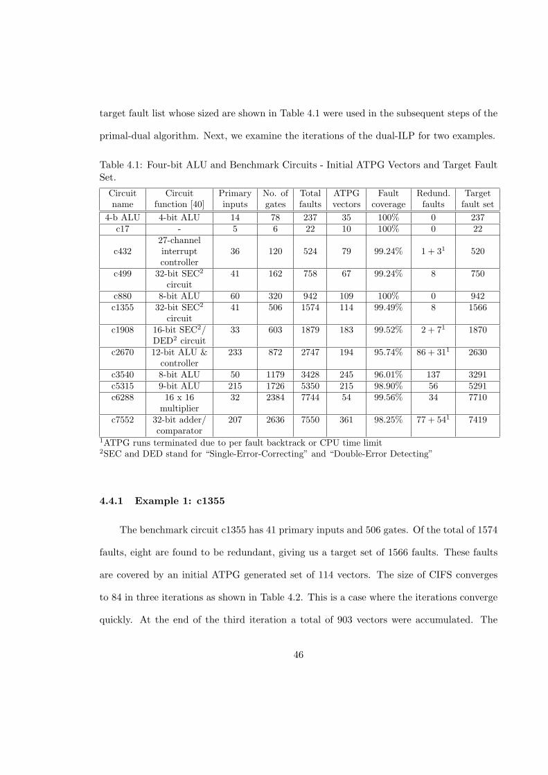
target fault list whose sized are shown in Table 4.1 were used in the subsequent steps of the

primal-dual algorithm. Next, we examine the iterations of the dual-ILP for two examples.

Table 4.1: Four-bit ALU and Benchmark Circuits - Initial ATPG Vectors and Target FaultSet.

Circuit Circuit Primary No. of Total ATPG Fault Redund. Targetname function [40] inputs gates faults vectors coverage faults fault set

4-b ALU 4-bit ALU 14 78 237 35 100% 0 237c17 - 5 6 22 10 100% 0 22

27-channelc432 interrupt 36 120 524 79 99.24% 1 + 31 520

controllerc499 32-bit SEC2 41 162 758 67 99.24% 8 750

circuitc880 8-bit ALU 60 320 942 109 100% 0 942c1355 32-bit SEC2 41 506 1574 114 99.49% 8 1566

circuitc1908 16-bit SEC2/ 33 603 1879 183 99.52% 2 + 71 1870

DED2 circuitc2670 12-bit ALU & 233 872 2747 194 95.74% 86 + 311 2630

controllerc3540 8-bit ALU 50 1179 3428 245 96.01% 137 3291c5315 9-bit ALU 215 1726 5350 215 98.90% 56 5291c6288 16 x 16 32 2384 7744 54 99.56% 34 7710

multiplierc7552 32-bit adder/ 207 2636 7550 361 98.25% 77 + 541 7419

comparator1ATPG runs terminated due to per fault backtrack or CPU time limit2SEC and DED stand for “Single-Error-Correcting” and “Double-Error Detecting”

4.4.1 Example 1: c1355

The benchmark circuit c1355 has 41 primary inputs and 506 gates. Of the total of 1574

faults, eight are found to be redundant, giving us a target set of 1566 faults. These faults

are covered by an initial ATPG generated set of 114 vectors. The size of CIFS converges

to 84 in three iterations as shown in Table 4.2. This is a case where the iterations converge

quickly. At the end of the third iteration a total of 903 vectors were accumulated. The

46

primal ILP selected exactly one vector per fault, giving a final set of 84 vectors. Considering

the published data on IFS [39, 45], this is the smallest possible test set. The results are

shown in Table 4.2.

Table 4.2: Example 1: Dual ILP Iterations and Primal ILP Solution for c1355.

Primal Iteration No. of ATPG Fault Sim. CIFS No. of min. ILPor dual number vectors CPU s CPU s Size vectors CPU s

1 114 0.033 0.333 85 0.24Dual 2 507 0.085 1.517 84 0.97

3 903 0.085 2.683 84 1.91Primal 903 84 3.38

4.4.2 Example 2: c2670

The benchmark circuit c2670 has 233 primary inputs and 872 gates. Of the total of

2747 faults, 86 are found to be redundant and 31 undetectable, giving us a target set of

2630 faults. These faults are covered by an initial ATPG generated set of 194 vectors. The

size of CIFS converges to a stable value of 70 in 12 iterations as shown in Table 4.3. This

is a case where the iterations do not converge quickly. At the end of the twelfth iteration a

total of 4200 vectors were accumulated. Even though this CIFS is larger than the published

results on IFS [39, 45], further iterations were suspended because the last three iterations

did not provide any reduction. The primal ILP selected exactly one vector per fault, giving

a final set of 70 vectors. Considering the published data on IFS [39, 45], this is not the

smallest possible test set, which might be more expensive to find. The results are shown

in Table 4.3. In this example, the size of CIFS is strongly dependent on the vector subset.

It indicates that we should explore different strategies for generating vectors for the dual

problem.

47

Table 4.3: Example 2: Dual ILP Iterations and Primal ILP Solution for c2670.

Primal Iteration No. of ATPG Fault Sim. CIFS No. of min. ILPor dual number vectors CPU s CPU s Size vectors CPU s

1 194 2.167 3.670 102 1.992 684 1.258 5.690 82 3.223 1039 1.176 6.895 79 7.904 1424 1.168 8.683 78 3.695 1738 1.136 10.467 76 5.89

Dual 6 2111 1.128 12.333 76 7.437 2479 1.112 14.183 74 7.168 2836 1.086 15.933 73 8.459 3192 1.073 17.717 72 9.8110 3537 1.033 19.267 70 10.9011 3870 1.048 20.983 70 12.0212 4200 1.033 22.600 70 13.44

Primal 4200 70 316.52

4.5 Benchmark Results

Benchmark circuit results obtained for the primal-dual ILP algorithm are summarized

in Table 4.4. The column Initial vectors gives number of vectors in the initial ATPG

generated test set. The column Final vectors gives the number of vectors accumulated after

dual ILP iterations. The next column gives the total CPU time taken for all the ATPG runs

and fault simulations performed during the dual ILP iterations. Recall that fault simulation

is required in every iteration of the dual ILP to generate the detection matrix needed for

ILP runs. The next three columns under the Dual-ILP Solution tab give the number of

dual ILP iterations, the final CIFS size obtained after the last dual ILP iteration, and the

CPU time for these iterations. The two columns under the Primal-ILP Solution tab give

the number of vectors in the minimized test set obtained as a solution to the primal ILP

and the CPU time for the primal ILP run. Here it can be seen that for larger benchmark

circuits the primal ILP runs are incomplete, and also the time taken by a single primal-ILP

48

Table 4.4: Test Sets Obtained by Primal-Dual ILP for 4bit ALU and Benchmark Circuits.

ATPG and Dual-ILP Primal-ILP solutionCircuit fault simulation solution with time-limitName Initial Final CPU No. of CIFS CPU Minimized CPU

vectors vectors s iterations size s vectors s

4b ALU 35 270 0.36 5 12 1.23 12 0.78c17 5 6 0.03 2 4 0.07 4 0.03c432 79 2036 1.9 13 27 25.04 30 2.2c499 67 705 2.41 4 52 2.33 52 1.08c880 109 1384 4.11 15 13 635.39 24 1001.06*c1355 114 903 2.89 3 84 1.21 84 3.38c1908 183 1479 7 4 106 10.79 106 19.47c2670 194 4200 34.85 12 70 91.9 70 316.52c3540 245 3969 24.76 9 84 622.09 104 1007.74*c5315 215 1295 13.83 5 39 510.82 71 1004.51*c6288 54 361 10.03 6 6 311.03 16 1004.3*c7552 361 4929 114 8 116 287.65 127 1015.06*

*Execution terminated due to a time limit of 1000 s

run is greater than the total time for the multiple dual ILP runs. Thus the computational

complexity of the dual ILP is much lesser than that of the primal ILP.

To examine the benefit of the primal-dual ILP over the plain (primal) ILP, we compare

the results of Table 4.4 with those in the literature [47]. In that work, ILP was used to

minimize large vector sets that were generated for N-detection. In some cases values of N

were greater than 100 resulting in large vector sets and therefore large numbers of variables

in ILP. That comparison is shown in Table 4.5. The principal benefit of the dual problem

appears to be in reducing the vector set size, which saves ATPG and fault simulation time,

as well as the ILP CPU time. It is also evident that the dual ILP takes much less CPU time

than the primal ILP. Hence, the use of the dual ILP in the iterative loop is appropriate,

while the primal ILP is used only once. Also, note that after the initial ATPG run that

includes all faults, all subsequent runs only work on CIFS that is much smaller.

49

Table 4.5: Comparing Primal-Dual ILP Solution With ILP-Alone Solution [47].

Circuit Lower bound ILP-alone minimization [47] Primal-dual minimization [this work]Name on vectors Unopt. LP Minimized Unopt. Total Minimized

[39, 45] vectors CPU s vectors vectors CPU s vectors

4b ALU 12 2370 5.19 12 270 2.01 12c432 27 14822 82.3 27 2036 27.24 30c499 52 397 5.3 52 705 3.41 52c880 13 3042 306.8 25 1812 1636.45* 24c1355 84 755 16.7 84 903 4.59 84c1908 106 2088 97 106 1479 30.26 106c2670 44 8767 1568.6* 71 4200 408.42 70c3540 78 - - - 3969 1629.83* 104c5315 37 - - - 1295 1515.53* 71c6288 6 243 519.7 18 361 1315.33* 16c7552 65 2156 1530.0* 148 4929 1302.71* 127

*ILP execution was terminated due to a CPU time limitNote: Both experiments were performed on SUN Fire 280R, 900 MHz Dual Core machine

4.6 Primal LP with Recursive Rounding

Due to the high computational complexity of the primal ILP, we transform it into a

linear program by treating the variables as real numbers in the range [0.0, 1.0]. We then

use the recursive rounding technique [48] to round off the real variables to integers. In the

recursive rounding method, the LP is recursively used, each time rounding off the largest

variable to 1 and reducing the size of the LP. This is done until an integer solution is

obtained. This is a polynomial time solution, but an absolute optimality is not guaranteed.

Table 4.6 gives test set sizes and CPU times for the primal-dual test minimization

method. Observe that the test sets obtained from the primal LP with recursive rounding

are smaller than those obtained by primal ILP (Table 4.4) for cases in which the primal ILP

gave suboptimal solution due to CPU time limited termination. Thus using primal LP with

recursive rounding is a good trade-off between optimality and computational complexity.

50

Table 4.6: Test Sets Obtained by Primal LP-Dual ILP Solution for 4bit ALU and Bench-mark Circuits.

Number of Dual-ILP solution Primal-LP solution TotalCircuit unoptimized with recursive rounding CPUName vectors No. of CIFS CPU Minimized CPU s

iterations size s vectors s

4b ALU 270 5 12 1.23 12 0.63 1.86c17 6 2 4 0.07 4 0.03 0.1c432 2036 13 27 25.04 30 1.14 27.28c499 705 4 52 2.33 52 0.43 3.41c880 1384 15 13 635.39 24 19.42 654.81c1355 903 3 84 1.21 84 0.82 4.59c1908 1479 4 106 10.79 107 0.38 30.26c2670 4200 12 70 91.9 70 10.73 102.3c3540 3969 9 84 622.09 95 99.75 721.84c5315 1295 5 39 510.82 63 298.5 809.32c6288 361 6 6 311.03 16 44.77 355.8c7552 4929 8 116 287.65 119 160.57 448.22

The graphs in Figures 4.2 and 4.3 give the comparison between primal LP-dual ILP

solution with Primal ILP-dual ILP solution. They illustrate the benefit of using the primal

LP over the primal ILP. The total CPU time for primal LP-dual ILP solution is significantly

lesser than the Primal ILP-dual ILP solution, whereas the test set sizes obtained are almost

similar for the two techniques.

Table 4.7 compares primal LP-dual ILP solution with the ILP-alone solution (recursive

LP version) [48] for almost similar unoptimized vector set sizes. For this reason, some

minimized vector sets in the last column are larger than those shown in Tables 4.4, 4.5

and 4.6. For example, in Table 4.7 the circuit c2670 has 79 vectors obtained after minimizing

a set of 1039 vectors. All other tables show 70 vectors for this circuit obtained from a set

4200 vectors that was generated by the dual ILP solution (Table 4.3). This observation

is significant because the level of compaction obtainable from the primal LP is dependent

on the type of vectors in the original vector set on which it is run. It is evident that

51

0

200

400

600

800

1000

1200

1400

1600

1800

c432 c880 C1355 C1908 C2670 C3540 C5315 C6288 C7552

ISCAS85 Benchmark Circuits

CP

U s

Primal-Dual ILP

Primal_LP-Dual_ILP

Figure 4.2: CPU Time Comparison Between Primal LP-Dual ILP Solution with Pri-mal ILP-Dual ILP Solution.

the primal-dual minimization technique performs better than the ILP-alone minimization

technique. This confirms the role of the dual ILP in obtaining proper vectors, which then

can be optimized by the primal LP. Note that the basic idea here is to target faults that

belong to an independent fault set.

4.7 Analysis of Duality for Integer Linear Programs

The duality theorem defined in Section 2.12 is applicable to linear programs [75]. How-

ever the concept of duality in the case of integer linear programs is not well understood

as no specific results are found in the literature. In this section we attempt to establish a

relation between the optimized values of the primal ILP and dual ILP.

In the previous section, we had seen that the primal ILP due to its high computational

complexity was transformed into a relaxed primal LP and solved using the recursive round-

ing technique. This transformation was done by allowing the variables to take on real values

52

0

20

40

60

80

100

120

140

c17 c432 c499 c880 C1355 C1908 C2670 C3540 C5315 C6288 C7552

ISCAS85 Benchmark Circuits

Nu

mb

er o

f V

ecto

rs

Primal-Dual ILP

Primal LP - Dual ILP

Figure 4.3: Test Set Size Comparison Between Primal LP-Dual ILP Solution with Pri-mal ILP-Dual ILP Solution.

in the range [0.0, 1.0]. Similarly, the dual ILP can also be transformed into a relaxed dual

LP problem. The Table 4.8 lists the optimized values for the objective functions obtained

from relaxed LP’s corresponding to both primal and dual ILP problems for the benchmark

circuits. Here the unoptimized vectors used were those shown in Tables 4.4 through 4.6,

and not those used for Table 4.7. The optimized values of the relaxed primal LP and the

relaxed dual LP are equal, which is in accordance with the duality theorem [75]. These

values are listed in the second column of Table 4.8.

It is also known that the optimized value of the objective function obtained from the

relaxed LP provides a bound for the parent ILP problem [46, 48]. Thus, the single value

obtained from primal and dual LP’s is an upper bound on the size of the conditional

independent fault set (CIFS) and is also a lower bound on the size of the minimized vector

53

Table 4.7: Comparing Primal LP-Dual ILP Solution with LP-Alone Solution [48].

Circuit Lower bound LP-alone minimization [48] Primal-dual minimization [this work]Name on vectors Unopt. LP Minimized Unopt. Total Minimized

[39, 45] vectors CPU s vectors vectors CPU s vectors

c432 27 608 2 36 983 5.52 31c499 52 379 1 52 221 1.35 52c880 13 1023 31 28 1008 227.21 25c1355 84 755 5 84 507 1.95 84c1908 106 1055 8 107 728 2.5 107c2670 44 959 9 84 1039 17.41 79c3540 78 1971 197 105 2042 276.91 95c5315 37 1079 464 72 1117 524.53 67c6288 6 243 78 18 258 218.9 17c7552 65 2165 151 145 2016 71.21 139

set. These bounds are expressed as follows:

Primal ILP objective ≥ Relaxed LP objective ≥ Dual ILP objective

Or

Minimized vector set size ≥ Relaxed LP objective ≥ Largest CIFS size

The data in Table 4.8 conforms to these inequalities. Because of the CPU time con-

straints, several primal ILP solutions (column 3) had to be obtained by the recursive round-

ing method [48]. These vector sets may be larger than the real optimum size that would be

possible if we could solve the ILP. Interestingly, in all such cases, the CIFS size (column 4)

is strictly lower than its upper bound. In most cases where the primal ILP was directly

solved, the CIFS size was equal to its upper bound.

54

Table 4.8: Comparison of Optimized Values of Relaxed LP and ILP.

Circuit Relaxed primal and Primal ILP Dual ILPName dual LP’s optimized objective finction objective function

objective functions (minimized vectors) (CIFS size)

4b-alu 12.00 12 12c17 4.00 4 4c432 29.06 30 27c499 52.00 52 52c880 19.53 24* 14c1355 84.00 84 84c1908 106.00 106 106c2670 70.00 70 70c3540 86.07 95* 84c5315 52.63 63* 39c6288 8.40 16* 6c7552 116.00 119* 116

*LP based recursive rounding [48]

Observe that in column 2 of Table 4.8, several entries (4b-alu, c17, c499, c1355, c1908,

c2670, and c7552) have integer values. Notably, these are the only cases where the CIFS

sizes (column 4) exactly match the upper bounds. With the exception of c7552, for all

circuits in this category, the minimized vector set size matched the respective lower bound.

In fact, we found that in the relaxed LP solutions for these circuits (excepting c7552) all

variables assumed only integer (0 or 1) values. Thus, the relaxed LP solutions were also the

ILP solutions. In some of these cases, theoretical lower bounds on vectors (see Table 4.7)

is actually achieved. Circuit c2670 is an exception that perhaps requires more, or better,

vectors to select from.

55

Chapter 5

Background on Fault Diagnosis

In this chapter we will review the different types of fault diagnosis techniques with

an emphasis on fault dictionary based diagnosis. We will also review the common fault

dictionary organizations, and a few compaction techniques employed to manage the size of

the fault dictionary.

5.1 Fault Diagnosis

The concept of fault diagnosis was introduced in Chapter 2. Fault diagnosis involves

applying tests to failed chips and analyzing the test results to determine the nature of the

fault. The results of fault diagnosis are suspected defect locations which are used to guide

the physical analysis process for defect identification. Diagnosis algorithms are broadly

classified into two types - cause-effect fault diagnosis and effect-cause fault diagnosis.

5.1.1 Cause-Effect Diagnosis

The cause-effect diagnosis starts with a particular fault model and compares the sig-

nature of the observed faulty behavior with the simulated signatures for each fault in the

circuit. A fault signature is the data representation of the response of a defective circuit to

a diagnostic test set [55]. Basically it is a list of failing vectors and the outputs at which

errors are detected. A cause-effect algorithm can further be classified as static, in which all

fault simulation is done in advance and all fault signatures are stored as a fault dictionary

or, as dynamic, where no pre-computed information is used and simulations are performed

56

only as needed during the diagnosis process. The single stuck-at fault model has been the

most widely used fault model in the area of fault diagnosis too.

As the cause-effect algorithms are based on a fault model and actual defects on the chip

may not behave according to the fault model used, the observed signature may not match

with any of the simulated signatures. In such cases sophisticated matching algorithms are

used to select a set of signatures that best match the observed signature [53].

5.1.2 Effect-Cause Diagnosis

As the name suggests the effect-cause algorithm directly examines the syndrome of the

failing chip and then derives the fault candidates [1] using path-tracing methods. The fault

candidate here usually is a logical location or area of the chip. Some of the effect-cause

diagnosis algorithms are structural pruning [80], backtrace (functional pruning) [52], inject

and evaluate [62], etc. One important feature of effect-cause diagnosis algorithms is that

they can be constructed to handle cases of multiple faults in the failing chip. This is an

advantage over most other diagnosis strategies that rely heavily on a single-fault assumption.

The diagnosis results of effect-cause algorithms are usually pessimistic and imprecise.

5.2 Diagnosis Using Fault Dictionaries

Fault dictionary based diagnosis has been very popular as it facilitates faster diagnosis

by comparing the observed behaviors with pre-computed signatures in the dictionary. This

is especially significant where a large number of parts must be diagnosed. Also, since fault

simulation is performed as a part of test generation, most test generation programs can

57

create a fault dictionary. When a fault dictionary is used for diagnosis, each entry (signa-

ture) in the dictionary must be compared with the observed behavior during the diagnosis

process. The comparison can be accomplished by changing the format of dictionary entries

to match the observed behavior or vice-versa. The choice depends on the dictionary format.

Most of the previously published approaches have implied that the observed behavior will

be converted into the dictionary entry format [19].

The two most popular forms of dictionaries are the full-response dictionary and the

pass-fail dictionary.

5.2.1 Full-Response (FR) Dictionary

The full-response dictionary is the most detailed form of fault dictionary which can

provide all the diagnosis information for a given test set. It consists of all output responses

of each fault for each test. Thus this dictionary for a modeled fault can not only tell what

test fails but also at which outputs discrepancies are observed. The size of such a dictionary

would be (F × V × O), where F is the number of faults, V number of vectors, and O is

the number of outputs. Thus the size of such a dictionary can get prohibitively large for

modern circuits.

Example: Let us consider a circuit with 2 outputs having 8 faults that are detected

by 5 test vectors. The fault free responses of the 5 tests are given in Figure 5.1. The

full-response dictionary obtained by complete fault simulation is shown in Figure 5.2.

5.2.2 Pass-Fail (PF) Dictionary

The pass-fail dictionary is the most compact form of fault dictionary. It stores a single

pass or fail bit for a fault-vector pair. The size of such a dictionary would be (F ×V ), where

58

Fault freeTests response

o1 o2t1 1 1t2 1 0t3 0 1t4 1 0t5 0 0

Figure 5.1: Tests and Their Fault Free Responses.

Output ResponsesFaults t1 t2 t3 t4 t5

f1 1 0 1 0 1 0 1 0 0 0f2 1 1 1 1 1 0 1 1 1 0f3 1 1 1 1 1 0 1 0 1 1f4 0 1 0 1 0 0 0 1 0 0f5 0 0 1 0 0 1 0 0 0 0f6 0 0 1 0 0 1 1 0 0 0f7 0 0 0 0 0 1 1 0 0 0f8 0 0 1 0 1 0 1 0 1 0

Figure 5.2: Full-Response Fault Dictionary.

F is the number of faults, and V the number of vectors. Thus the size of a PF dictionary

is independent of the number of outputs of a circuit and is a lot smaller than the FR

dictionary. However, the disadvantage with pass-fail dictionaries is that since the failing

output information is ignored, faults that fail same set of tests but at different outputs

cannot be distinguished [54]. Thus pass-fail dictionaries are not commonly used for fault

diagnosis.

The pass-fail dictionary for the circuit in the example of the previous section is shown

in Figure 5.3. Here ‘0’ stands for pass and ‘1’ stands for fail.

59

t1 t2 t3 t4 t5f1 1 0 1 0 0f2 0 1 1 1 1f3 0 1 1 0 1f4 1 1 1 1 0f5 1 0 0 1 0f6 1 0 0 0 0f7 1 1 0 0 0f8 1 0 1 0 1

Figure 5.3: Pass-Fail Fault Dictionary.

5.3 Dictionary Compaction

There has been a lot of work done to reduce the size of the full-response dictio-

nary [19, 54, 61]. Most of these techniques concentrate on reducing the size by managing

the organization and encoding of the dictionary. Dictionary organization is the order and

content of the information. Basically it tells us what data is stored in the dictionary. Dic-

tionary encoding is the data representation format in the dictionary, i.e., how the data is

stored in the dictionary. An appropriate organization and encoding is essential in making

dictionary-based diagnosis practical for very large circuits.

On one extreme is the detailed FR dictionary that contains all the information to

diagnose every diagnosable fault and on the other extreme is the compact PF dictionary

that may not distinguish all the distinguishable faults. The compaction techniques search

for a dictionary in between these two dictionaries. They look for the smallest dictionary

that can give a diagnostic resolution of a FR dictionary.

Pomeranz and Reddy in [61] have given an algorithm by which sufficient amount of

information can be added to a pass-fail dictionary to obtain a resolution equal to the

resolution of the full-response dictionary. Their method uses a greedy algorithm to choose

columns from a full-response dictionary to augment a pass-fail dictionary.

60

Another popular method of compacting is to only record the failing output vectors.

Since it is unlikely that all faults will be detected by all tests, many output vectors will

be fault free. Therefore we can drop a lot of unnecessary information without sacrificing

the diagnostic resolution. Such a dictionary is called a detection dictionary. In its full

form, the detection dictionary contains all the information present in a FR dictionary. One

drawback of such a dictionary is that the structure becomes irregular, which inhibits the

encoding of the dictionary entries. This dictionary can be further compacted by sacrificing

the diagnostic resolution using a drop-on-K heuristic. A drop-on-K detection dictionary

is one where the number of detections for each fault is limited to K. Another variation of

drop-on-K is a drop-when-distinguished dictionary.

The paper by Higami et al. [41] describes an algorithm to compact the diagnostic vector

set used in a pass-fail dictionary, thereby reducing the dictionary size. The algorithm for

compaction is based on a set covering method. They use a fault distinguishing table (FDIST)

which contains information about fault pairs distinguished by each vector. However, since

the number of fault pairs is usually very large, a complete FDIST cannot be constructed

and stored. Thus they work with a partial FDIST which includes information only for a

subset of all possible fault pairs. Using the partial FDIST, a small number of vectors is

selected. Then fault simulation is performed for the selected vectors to see if the original

diagnostic resolution is achieved. If not another subset of fault pairs is selected and a

new partial FDIST is constructed for the newly selected fault pairs and additional test

vectors are selected. This process is repeated until all the distinguishable fault pairs are

distinguished. The paper does not describe the set covering method used in the algorithm.

And the algorithm is for a PF dictionary which is not commonly used due its low diagnostic

61

resolution. This was the only work on diagnostic vector set compaction that we could find

in the literature.

62

Chapter 6

Daignostic Test Set Minimization

In this chapter we give an Integer Linear Program (ILP) formulation to minimize

test sets for a full-response dictionary based diagnosis. The ILP formulation is an exact

solution and has high complexity in terms of number of constraints. Next, we introduce a

generalized fault independence relation to reduce the number of constraints in the diagnostic

ILP. Finally a two-phase method is proposed for generating a minimal diagnostic test set

from any given test set.

6.1 ILP for Diagnostic Test Set Minimization

In the previous chapter we had seen two ILP formulations - Primal ILP for minimizing

a detection test set and Dual ILP to find the largest IFS. Both of these use a fault detection

table which contains information about faults detected by each vector. The fault detection

table was obtained by fault simulation without fault dropping. Note that the information

in a fault detection table is similar to that in the pass-fail dictionary.

6.1.1 Fault Diagnostic Table for Diagnostic ILP

The ILP formulation for minimizing test sets used for full-response dictionary based

diagnosis will have to use a matrix which not only tells what tests detect which faults,

but also at which outputs the discrepancies were observed for each fault-test pair. For this

reason we use a fault diagnostic table. We illustrate the construction of a fault diagnostic

table with the following example.

63

Output ResponsesFaults t1 t2 t3 t4 t5

f1 1 0 1 0 1 0 1 0 0 0f2 1 1 1 1 1 0 1 1 0 0f3 1 1 1 1 1 0 0 0 0 0f4 0 1 0 1 0 0 0 1 0 0f5 0 0 0 0 0 1 0 0 1 1f6 0 0 0 0 0 1 0 0 0 0f7 0 0 0 0 0 1 0 0 0 1f8 0 0 1 0 1 0 1 0 0 0

Figure 6.1: Full-Response Fault Dictionary.

t1 t2 t3 t4 t5f1 1 1 1 1 0f2 2 2 1 2 0f3 2 2 1 0 0f4 3 3 0 3 0f5 0 0 2 0 1f6 0 0 2 0 0f7 0 0 2 0 2f8 0 1 1 1 0

Figure 6.2: Fault Diagnostic Table.

Let us consider a circuit with 2 outputs having 8 faults that are detected by 5 test

vectors. A sample full response dictionary for such a circuit is shown in the Figure 6.1.

Here ‘0’ stands for pass and ‘1’ stands for fail.

We use integers to represent the output response for each test vector. As faults de-

tected by different test vectors are already distinguished, there is no need to compare the

corresponding output responses. Hence we assign indices for the failing output responses for

each test vector. In the example, for test t1 the 3 different failing output responses (“10”,

“11”, and “01”) are indexed by integers 1, 2, and 3, respectively, in the fault diagnostic

table as shown in Figure 6.2. The largest integer needed to index an output response in

the worst case is equal to minimum(2No. of output pins − 1, highest number of faults detected

64

by any test vector). However it should be noted that output responses to a particular vector

are likely to repeat across a fault set as faults in the same output cone can have identical

output responses for a particular test. For this reason the largest integer needed to index

an output response observed in our experiments was much smaller than the highest number

of faults detected by any test vector.

6.1.2 Diagnostic ILP Formulation

Suppose a combinational circuit has K faults. We are given a vector set V of J vectors

and we assign a [0, 1] integer variable vj , j = 1, 2, . . . , J to each vector. The variables

vj have the following meaning:

• If vj = 1, then vector j is included in the selected vector set.

• If vj = 0, then vector j is discarded.

Without loss of generality, we assume that all K faults are detected by vector set V and

are also distinguishable from each other. Our problem then is to find the smallest subset of

these vectors that distinguish all the fault pairs. We simulate the fault set and the vector

set without dropping faults and the fault diagnostic table is constructed as explained in the

previous section. In this table, an element akj ≥ 1 only if fault k is detected by vector j.

The diagnostic ILP problem is stated as,

MinimizeJ

∑

j=1

vj (6.1)

subject to,

65

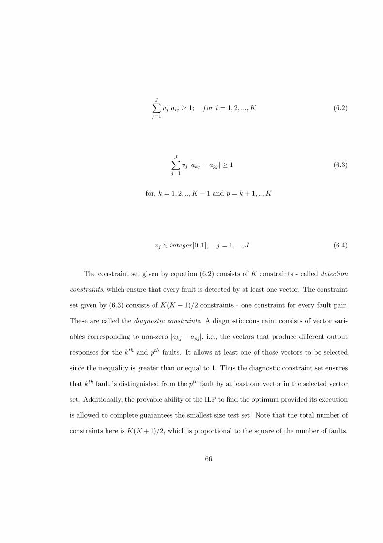
J∑

j=1

vj aij ≥ 1; for i = 1, 2, ..., K (6.2)

J∑

j=1

vj |akj − apj | ≥ 1 (6.3)

for, k = 1, 2, .., K − 1 and p = k + 1, .., K

vj ∈ integer[0, 1], j = 1, ..., J (6.4)

The constraint set given by equation (6.2) consists of K constraints - called detection

constraints, which ensure that every fault is detected by at least one vector. The constraint

set given by (6.3) consists of K(K − 1)/2 constraints - one constraint for every fault pair.

These are called the diagnostic constraints. A diagnostic constraint consists of vector vari-

ables corresponding to non-zero |akj − apj |, i.e., the vectors that produce different output

responses for the kth and pth faults. It allows at least one of those vectors to be selected

since the inequality is greater than or equal to 1. Thus the diagnostic constraint set ensures

that kth fault is distinguished from the pth fault by at least one vector in the selected vector

set. Additionally, the provable ability of the ILP to find the optimum provided its execution

is allowed to complete guarantees the smallest size test set. Note that the total number of

constraints here is K(K +1)/2, which is proportional to the square of the number of faults.

66

t1 t2 t3 t4f1 1 0 1 0f2 1 1 0 0f3 0 0 1 1

Figure 6.3: Fault Detection Table.

6.2 Generalized Fault Independence

One clear disadvantage of the diagnostic ILP is that the number of constraints is a

quadratic function of the number of faults. Thus for large circuits the number of con-

straints would be unmanageable. To overcome this, we define a relation between a pair of

faults which allows us to drop the diagnostic constraints in the ILP corresponding to such

fault pairs. We have generalized the conventional fault independence given in literature by

considering the detection of the faults at different outputs and relative to a vector set. In [7],

a pair of faults is called independent if the faults are not detected by a common vector. This

definition does not take into account the detection of the faults at specific outputs. Also

it implies “absolute” independence, which is conditional to the exhaustive vector set. We

generalize the definition of fault independence by saying that two faults detected by the

same vector can still be called independent, provided the output responses of the two faults

to that vector are different.

Definition 3: Generalized Fault Independence - A pair of faults detectable by a vector

set V are said to be independent with respect to vector set V, if there is no single vector that

detects both the faults and produces an identical output response.

Note that the generalized independence relation is conditional to a vector set.

Example: Consider a fault detection table with 3 faults and 4 test vectors as shown in

Figure 6.2. The independence relation between every fault pair is given in Table 6.2.

67

Table 6.1: Independence Relation.Fault Independence Reasonpair relationf1, f2 NO Both faults

detected by t1f1, f3 NO Both faults

detected by t3f2, f3 YES No vector detects

both faults

t1 t2 t3 t4f1 1 0 1 0f2 2 1 0 0f3 0 0 1 1

Figure 6.4: Fault Diagnostic Table.

Table 6.2: Generalized Independence Relation.Fault Generalized Reasonpair Indep. relation

Different outputf1, f2 YES responses for t1

detecting both faultsIdentical output

f1, f3 NO responses for t3detecting both faults

f2, f3 YES No vector detectsboth faults

68

Table 6.3: Constraint Set Sizes.

No. of Initial No. of FinalCircuit Faults Constraint Diagnostic Constraint

Set Indep. Flt. SetPairs

4 alu 227 25,651 22,577 3,074c17 22 231 170 61c432 520 125,751 111,589 14,162c499 750 271,953 138,255 133,698c880 942 392,941 344,180 48,761c1908 1870 1,308,153 1,201,705 106,448

Now consider a fault diagnostic table for the same set of faults and vectors as shown in

Figure 6.2. Recall that the fault diagnostic table takes into account the output responses

for each fault-vector pair. It is constructed as explained in Section 6.1.1. The generalized

independence relations for all pairs of faults are given in Table 6.2.

In the context of the diagnostic ILP, the generalized independence relation plays an

important role in reducing the number of constraints to be used in the formulation. When

two faults are independent, any vector that detects either of the faults will be a distinguish-

ing vector for the two faults. Thus, in the constraint set of equation (6.3), a constraint for

an independent fault pair will have vector variables corresponding to all the vectors that

detect any one or both the faults. In the presence of detection constraints of equation (6.2)

which guarantee a test for every fault, a diagnostic constraint for an independent fault

pair is redundant. Also, such a constraint will be covered by other diagnostic constraints

corresponding to non-independent fault pairs containing a fault from the independent fault

pair.

Table 6.3 shows the reduction in the constraint set sizes by considering generalized

independent faults for a 4 bit ALU and few ISCAS85 benchmark circuits.

69

It can be seen that there is an order of magnitude reduction in the constraint set sizes

on eliminating constraints corresponding to diagnostic independent faults. However the

constraint set sizes still are large and need to be reduced to manageable proportions. We

further address this problem in the next section.

6.3 Two-Phase Minimization

Given an unoptimized test set, we propose the following procedures:

Phase 1: Use existing ILP minimization techniques [73, 29] to obtain a minimal detection

test set from the given unoptimized test set. Find the faults not diagnosed by the minimized

detection test set.

Phase 2: Run the diagnostic ILP on the remaining unoptimized test set to obtain a minimal

set of vectors to diagnose the undistinguished faults from phase-1. The resulting minimized

test set combined with the minimal detection test set of phase-1 serves as a complete diag-

nostic test set.

In the context of diagnostic ILP of phase-2, the phase-1 along with the generalized

independence relation helps in reducing the number of constraints to manageable levels.

This is because diagnostic constraints are now needed only for the undiagnosed fault pairs

of phase-1. Also, there will be a further reduction in the number of diagnostic constraints

due to diagnostically independent fault pairs that could be present. We can also drop

the detection constraints as we have started with a detection test set that detects all the

targeted faults.

70

There is another benefit of the test set obtained by the two-phase approach. For all

good chips, testing can be stopped at the detection test set, which is of minimal size.

Only for bad chips whose number depending on yield may be small, we need to apply the

remaining tests for diagnosis.

The graph in Figure 6.5 gives the comparison between diagnostic test sets got by

single-step diagnostic ILP minimization and the 2-phase approach. The experiment could

be performed only on 4-b ALU and the smaller benchmark circuits c17 and c432. For other

larger benchmark circuits like c880 we could not run the diagnostic ILP as the number of

constraints was too many for the problem to be loaded onto the computer. Hence the empty

slot in the graph for the 1-step process of c880. As can be seen, the final diagnostic test

sets obtained by 2-phase approach are slightly larger than the ones obtained by single-step

minimization. In the case of 2-phase minimization, we had suggested that the testing of

good chips can be stopped at the minimal detection test set and the remaining diagnostic

tests (which are few) can be used to complete the diagnosis of bad chips. This idea can

applied to the diagnostic test set got by single-step diagnostic ILP. A detection test set

can be obtained from the vectors comprising the diagnostic test set by using the existing

ILP minimization techniques [29] (Test minimization ILP). The diagnostic vector set can

be reordered such that the detection vectors are present at the start of the vector set.

Thus here too the testing of good circuits can be stopped at the detection vector sets. It

can be seen from the graph that, for c17, 4-b ALU and c432 the detection test set in the

case of single-step diagnostic ILP minimization is larger than that obtained during 2-phase

minimization. Thus the testing of good circuits will take a longer time, which depending

71

0

10

20

30

40

50

60

Nu

mb

er o

f V

ecto

rs

1-step 2-phase 1-step 2-phase 1-step 2-phase 1-step 2-phase

ALU and Benchmark Circuits

Additional Diagnostic Vectors

Detection Vectors Complete Diagnostic

Test Set

4 - b ALU c17 c432 c880

0

10

20

30

40

50

60

Nu

mb

er o

f V

ecto

rs

1-step 2-phase 1-step 2-phase 1-step 2-phase 1-step 2-phase

ALU and Benchmark Circuits

Additional Diagnostic Vectors

Detection Vectors Complete Diagnostic

Test Set

4 - b ALU c17 c432 c880

Figure 6.5: Comparison Between 1-Step Diagnostic ILP Minimization and 2-Phase Ap-proach

on the yield may be high in number. The complete diagnostic test set will be applied to

only to bad circuits, which in case of high yield are few.

6.4 Results

In our experiments we have used the ATPG ATALANTA [56] and fault simulator

HOPE [57]. We have used AMPL package [30] for ILP formulation.

Results of phase-1 are given in Table 6.4. First column lists the names of the ISCAS85

circuits. The next column gives the number of faults in the target fault list. These faults

are equivalence collapsed single stuck-at faults, excluding the ones that were identified as

redundant or were aborted by the ATPG program. We have used the minimal detection

test sets obtained using the primal-dual test minimization algorithm of Section 4.6. The

primal-dual algorithm creates unoptimized test sets which essentially consist of N-detect

tests, and then minimizes them to give the minimal detection test sets. The sizes of the

72

unoptimized and minimized vector sets are given in columns 3 and 4 of the table. The

subsequent columns give the diagnosis statistics of the minimal detection test sets. We

say a fault is uniquely diagnosed if it has a unique syndrome. On the other hand a fault

whose syndrome is shared by other faults is said to be undiagnosed. Column 5 gives the

number of undiagnosed faults. Faults with identical syndromes are grouped into a single

set called an equivalent fault set. Note that such an equivalent fault set is dependent

on the vector set used for diagnosis, thus it is called a Conditional Equivalent Fault Set

(CEFS). The column, No. of CEFS gives the number of such sets. There is one CEFS

for every non-unique syndrome consisting of the undiagnosed faults associated with that

syndrome. Maximum faults per syndrome give the maximum number of faults associated

with a syndrome. Diagnostic resolution (DR) defined in [3] gives an average number of

faults per syndrome. It is obtained by dividing the total number of faults by the total

number of syndromes. These two parameters quantify the effectiveness of diagnosis since

DR indicates how well faults are distributed among all syndromes and the Maximum faults

per syndrome indicate the worst distribution among all syndromes. The undiagnosed faults

obtained in this step are the target faults in phase-2 of our algorithm.

Table 6.5 gives the results for phase-2 in which diagnostic ILP is used to minimize

the tests for the undistinguished fault pairs of phase-1. In this step we have used the

unoptimized test sets (excluding the minimal detection tests) of phase-1. The No. of Faults

here are the undiagnosed faults from Table 6.4. The next column gives the number of

constraints generated during the ILP formulation. It can be seen that the constraint set

size is very small even for the larger benchmark circuits like c7552 and c6288. The column

Minimized Vectors gives the result of the diagnostic ILP. These vectors combined with the

73

Table 6.4: Phase-1: Diagnosis With Minimal Detection Test Sets.

No. of Primal-Dual Minimal Detection Test Diagnostic StatisticsCircuit Faults Algorithm [73]

No. of No. of No. of No. of Maximum DiagnosticUnoptim. Minimized Undiagnosed CEFS Faults per ResolutionVectors Vectors Faults Syndrome

4b ALU 227 270 12 43 19 4 1.118c17 22 32 4 6 3 2 1.158c432 520 2036 30 153 68 9 1.195c499 750 705 52 28 12 3 1.023c880 942 1384 24 172 83 4 1.1c1355 1566 903 84 1172 531 5 1.693c1908 1870 1479 107 543 248 17 1.187c2670 2630 4200 70 833 316 11 1.245c3540 3291 3969 95 761 313 8 1.158c5315 5291 1295 63 1185 527 8 1.142c6288 7710 361 16 2416 1122 6 1.202c7552 7419 4924 122 1966 891 7 1.17

minimal detection vectors of phase-1 constitute the complete diagnostic test set. The last

column gives the CPU time for the diagnostic ILP runs. It is evident that the complexity

of the diagnostic ILP is greatly reduced. All CPU times are for a SUN Fire 280R 900MHz

Dual Core machine. For cases in which the ILP complexity is high, reduced-complexity LP

variations described in [48] can be used.

Table 6.6 gives the results and statistics of the fault dictionary obtained by using the

complete diagnostic test set. The total diagnostic vectors are the combined vector sets from

phase-1 and 2. Notice that these test sets are just a little bigger than the minimal detection

test sets of Table 6.4. Thus failed chips can be diagnosed very quickly as the detection

tests would have already been applied during testing. Column 3 gives the number of faults

in the target fault list. Column 4 gives the number of uniquely diagnosed faults. The

remaining columns have similar meaning to that of Table 6.5. It can be seen that there

74

Table 6.5: Phase-2: Diagnostic ILP Minimization.

Circuit Number of No. of No. of Minimized CPU sUnoptimized Vectors Faults Constraints Vectors

4b ALU 258 43 30 6 1.36c17 28 6 3 2 1.07c432 2006 153 101 21 3.03c499 652 28 10 2 1.09c880 1358 172 41 7 2.74c1355 1131 1172 12 2 2.13c1908 819 543 186 21 3.16c2670 4058 833 383 51 5.29c3540 3874 761 146 27 8.45c5315 1232 1185 405 42 15.35c6288 345 2416 534 12 50.13c7552 4802 1966 196 31 9.35

is an improvement in the diagnostic resolution from that of phase-1 due to the diagnosis

vectors from phase-2.

The unoptimized test sets used in our experiments are essentially N-detect tests. It

should be noted here that using an unoptimized test set consisting of diagnostic ATPG

vectors [79] will be more effective in achieving a good diagnostic resolution, as these vectors

are generated for the sole purpose of distinguishing pairs of faults.

Table 6.7 gives the comparison between our work on two-phase minimization and a prior

work [41] on the compaction of test sets for a pass-fail dictionary. For both the algorithms

an initial unoptimized set of 1024 random vectors is used. The authors in [41] measure

the diagnostic effectiveness of the compacted test set in terms of number of undiagnosed

fault pairs. The pass-fail dictionaries have inherently lower resolution than the full-response

dictionaries. Thus there may not be a one-to-one comparison between these results as the

prior work is for a pass-fail dictionary test set and ours is for a full-response dictionary.

75

Table 6.6: Diagnosis with Complete Daignostic Test Set.

1 2 3 4 5 6 7 8 9Total No. of Uniquely No. of Undiag. No. of Maximum Diagnostic

Circuit Diag. Faults Diag. CEFS faults Synd. Faults per ResolutionVectors Faults (3 - 4) (4 + 5) Syndrome (3 / 7)

4b ALU 18 227 227 0 0 227 1 1c17 6 22 22 0 0 22 1 1c432 51 520 488 16 32 504 2 1.032c499 54 750 726 12 24 738 2 1.016c880 33 942 832 55 110 887 2 1.062c1355 86 1566 397 532 1169 929 3 1.686c1908 127 1870 1380 238 490 1618 8 1.156c2670 121 2630 2027 263 603 2290 11 1.149c3540 122 3291 2720 234 571 3033 8 1.085c5315 105 5291 4496 381 795 4877 4 1.085c6288 28 7710 5690 1009 2020 6699 3 1.151c7552 153 7419 5598 848 1821 6446 7 1.151

However we can notice the compactness of the diagnostic test sets got by the two-phase

method and its computing efficiency.

6.5 Analysis of Undistinguished Fault Pairs of c432

We examine the fault pairs that remained undistinguished by the minimized diagnostic

vector set. From Table 6.6 we see that for c432 the minimized diagnostic test set has 51

vectors and the number of undiagnosed faults is 32, which are distributed in 16 conditional

equivalent fault sets (CEFS). Now, since the maximum faults per syndrome is 2, each CEFS

can contain at most 2 faults. Thus there are 16 undistinguished fault pairs.

We used the circuit structure shown in Figure 6.6 to examine the undistinguishable

fault pairs. Here, two copies of the circuit under test (CUT) are used. Each copy has one

fault from the fault pair permanently inserted. Both copies have the same primary inputs

and their outputs are connected as shown in Figure 6.6 to derive a primary output for

76

Table 6.7: Two-phase Minimization vs. Previous Work [41].

Pass-Fail dictionary compaction [41] Two-Phase Approach [This work]Circuit Fault Minim. Undist. CPU Fault Minim. Undist. CPU

Coverage Vectors Fault s Coverage Vectors Fault s% Pairs % Pairs

c432 97.52 68 93 0.1* 98.66 54 15 0.94**c499 - - - - 98.95 54 12 0.39**c880 97.52 63 104 0.2* 97.56 42 64 2.56**c1355 98.57 88 878 0.8* 98.6 80 766 0.34**c1908 94.12 139 1208 2.1* 95.69 101 399 0.49**c2670 84.4 79 1838 2.8* 84.24 69 449 8.45**c3540 94.49 205 1585 10.6* 94.52 135 590 17.26**c5315 98.83 188 1579 15.4* 98.62 123 472 25.03**c6288 99.56 37 4491 1659* 99.56 17 1013 337.89**c7552 91.97 198 4438 33.8* 92.32 128 1289 18.57**

*Pentium IV 2.6 GHz machine **SUN Fire 280R, 900 MHz Dual Core machine

the composite circuit. An ATPG is used to detect sa0 fault at the primary output of the

composite circuit. There are three possible outcomes of the ATPG run.

1. An exclusive test is found indicating that the faults are distinguishable. An Exclusive

test is an input vector that detects only one fault from a pair of targeted faults [3].

2. Identifies the output sa0 fault as redundant, in which case the two faults fi and fj are

equivalent. Although not often recognized, all redundant faults of a combinational

circuit form an equivalent fault set.

3. Aborts - no conclusion can be reached on the distinguishablity of faults in the fault

pair.

For c432, after running the ATPG for the 16 fault pairs, an exclusive test was found

for 3 pairs, and for the remaining 13 pairs the ATPG aborted. This illustrates the need for

programs to generate exclusive tests for fault pairs. Also, efficient programs are needed to

find functional equivalences.

77

CUT f i

CUT f j

x s a0

1

1

n

n

Primary Inputs

Figure 6.6: An ATPG-based Method for Examining a Fault Pair (fi, fj).

For c432, we added the 3 vectors obtained as exclusive tests to the original test set

of 2036 vectors and repeated the 2-phase minimization. Phase-1 gave a minimal detection

test set of 30 vectors which is the same as that obtained in the earlier 2-phase minimization

run of Table 6.4. Phase-2 gave a minimal diagnostic set of 23 additional vectors, 2 more

than the earlier case (Table 6.5). Thus, the new complete diagnostic test set consisted of

53 vectors and the 26 faults (i.e., 13 fault pairs) remained undiagnosed.

78

Chapter 7

Conclusion

The initial part of this thesis gives a dual ILP formulation, which is an exact solution to

finding the maximal IFS. The dual ILP is modeled as the dual of the test minimization ILP

(now called the primal ILP) described in literature. It was observed that the computational

complexity of the dual ILP was much lesser than that of the primal ILP. Using the primal

ILP and dual ILP we have presented a novel primal-dual algorithm for test optimization

for combinational circuits. The dual ILP helps in obtaining proper vectors, which then

can be optimized by the primal ILP. We should point out that the ILP formulation for

both the primal and dual is exact and has exponential complexity. As the primal ILP was

more complex than the dual, for larger benchmark circuits we see large CPU times. Thus

in place of primal ILP, we use primal LP based recursive rounding technique which is of

lower complexity and provides an approximate solution. The primal-dual method, when

applied to the ISCAS85 benchmark circuits, produced better results compared to an earlier

LP-alone test minimization method [47].

In the second part of the thesis we have presented an Integer Linear Program (ILP)

formulation for compaction of the diagnostic test set used in full-response dictionary based

fault diagnosis. The compaction can be carried out without any loss in the diagnostic

resolution of the initial test set. The newly defined diagnostic independence relation between

pairs of faults is very effective in reducing the number of faults that need to be distinguished,

thereby reducing the number of constraints in the diagnostic ILP. Finally we have proposed

a 2-phase approach for generating a minimal diagnostic test set. The diagnostic test sets

79

obtained are very small because of which there can be a significant reduction in the fault

dictionary size and also the diagnosis time.

7.1 Future Work

• In the context of primal-dual algorithm of Chapter 4, Theorem 2 [73] suggests that as

the vector set approaches the exhaustive set, the CIFS must converge to IFS. In our

experiments it was observed that for dual ILP iterations using N-detect vectors for

the faults in the CIFS made the convergence of the CIFS to the IFS a slow process.

Thus, new strategies for generating vectors for the dual problem must be explored in

order to have the CIFS quickly converge to IFS before vector set becomes exhaustive.

• Yogi and Agrawal’s work on N-model test set minimization [81], showed how a single

detection table can be constructed for tests of multiple fault models. This idea could

be used for creating a fault dictionary for multiple fault models and then using the 2-

phase approach to minimize the diagnostic vector set. The diagnosis results of such a

fault dictionary could be more accurate in predicting the defect locations and nature.

• Toward improving the resolution of diagnostic tests, the analysis of the undiagnosed

fault pairs of c432 in Section 6.5 showed the need for programs to generate exclusive

tests for fault pairs. Also, efficient programs are needed to find functional equivalences.

7.1.1 Primal-Dual Algorithm with Partially Specified Vectors

Consider the circuit consisting of two AND gates as shown in Figure 7.1. The faults in

the figure are equivalence collapsed single stuck-at faults. Suppose that vectors t1, t2 and

t3 are generated by targeting faults of the first AND gate, and vectors t4, t5, and t6 are

80

sa1

sa1

sa0 x x

x

x

sa1

sa1

sa0 x

x x x

sa1

sa1

1

2

1 1 0 0

1 0 1 0

0 1 1 0

0 0 1 1

1 1 0 0

1 0 1 0

0 1 1 0

0 0 1 1

Minimized Vector Set

0 1 1

1 0 1

0 1 0

0 0 0

0 1 1

1 0 1

0 1 0

0 0 0

0 0 1

0 0 0

0 1 1

1 0 1

ATPG Vectors

t6 t5 t4 t3 t2 t1

Figure 7.1: Non-optimal Solution Obtained Using ILP Minimization.

generated by targeting faults of the second AND gate. Now the ILP minimization of the 6

vectors gives us a test set of 4 vectors. But this circuit has a minimal detection test set of

3 vectors.

We used the primal-dual algorithm on similar circuits consisting of 4, 8 and 16 AND

gates. It was observed the algorithm could find a minimal test set of 4 vectors for all the

three circuits by minimizing vectors accumulated in two dual ILP iterations. But it did not

get to the absolute minimal set of 3 vectors even after seven dual ILP iterations.

Figure 7.2 shows a possible solution to the problem illustrated above. Here ILP min-

imization is carried out for partially specified test vectors, followed by further compaction

of the minimized test set by vector merging. A partially specified vector is one in which

the bits corresponding to unspecified inputs are left as X’s (don’t cares). Vector merging

is a static compaction technique where pairs of partially specified test vectors, that do not

conflict in their specified (0, 1) values, are repeatedly merged into single vectors [13]. We

81

sa1

sa1

sa0 x x

x

x

sa1

sa1

sa0 x

x

0 1 1

1 0 1

x x x

x x x

0 1 1

1 0 1

x x x

x x x

x x x

x x x

0 1 1

1 0 1 x x

sa1

sa1

1

2

Compacted Vector Set

0 1 1

1 0 1

0 1 1

1 0 1

0 1 1

1 0 1

0 1 1

1 0 1

x x x 0 1 1

x x x 1 0 1

0 1 1 x x x

1 0 1 x x x

Minimized Vector Set t3 t2 t1 t6 t5 t4

Figure 7.2: Minimizing Partially Specified Vectors and then Vector Merging.

start with the six partially specified vectors and then minimize them using the ILP min-

imization. We have found that an ILP formulation for partially specified vectors can be

easily worked out. In this example the ILP minimization does not provide any reduction in

initial test set size. This is because the circuit used here is an extreme example. Normally,

there will be reduction in the test set size. However, the level of compaction achievable by

ILP minimization may not be as high as in the case of fully specified vectors. On further

compacting the vectors resulting from ILP minimization we get a set of 3 vectors, which is

the minimal possible set for this circuit.

A similar approach can be used for the primal-dual algorithm. We can use primal-dual

algorithm with partially specified vectors. Then the resulting minimized test set is further

compacted by vector merging. Such an approach may produce more compact test sets.

The use of partially specified vectors and ILP minimization followed by don’t care merging

may be especially beneficial for circuits with small logic depth and large number of primary

inputs.

82

Bibliography

[1] M. Abramovici and M. A. Breuer, “Multiple Fault Diagnosis in Combinational Circuits Basedon an Effect-Cause Analysis,” IEEE Transactions on Computing, vol. C-29, no. 6, pp. 451–460,June 1980.

[2] V. D. Agrawal and P. Agrawal, “An Automatic Test Generation System for Illiac IV LogicBoards,” IEEE Trans. on Computers, vol. C-21, no. 9, pp. 1015–1017, Sept. 1972.

[3] V. D. Agrawal, D. H. Baik, Y. C. Kim, and K. K. Saluja, “Exclusive Test and its Applicationsto Fault Diagnosis,” in Proc. International Conf. on VLSI Design, 2003, pp. 143–148.

[4] V. D. Agrawal, A. V. S. S. Prasad, and M. V. Atre, “Fault Collapsing via Functional Domi-nance,” in Proc. International Test Conf., 2003, pp. 274–280.

[5] V. D. Agrawal, A. V. S. S. Prasad, and M. V. Atre, “It is Sufficient to Test 25-Percent ofFaults,” in Proc. Seventh IEEE VLSI Design and Test Workshop, 2003, pp. 368–374.

[6] V. D. Agrawal and S. C. Seth, Test Generation for VLSI Chips. Los Alamitos, CA: IEEEComputer Society Press, 1988.

[7] S. B. Akers, C. Joseph, and B. Krishnamurthy, “On the Role of Independent Fault Sets in theGeneration of Minimal Test Sets,” in Proc. International Test Conf., 1987, pp. 1100–1107.

[8] S. B. Akers and B. Krishnamurthy, “Test Counting: A Tool for VLSI Testing,” IEEE Designand Test of Computers, vol. 6, no. 5, pp. 58–77, Oct. 1989.

[9] D. B. Armstrong, “A Deductive Method for Simulating Faults in Logic Circuits,” IEEE Trans-actions on Computers, vol. C-21, no. 5, pp. 464–471, May 1972.

[10] S. P. Bradley, A. C. Hax, and T. L. Magnanti, Applied Mathematical Programming. Addison-Wesley, 1977.

[11] F. Brglez, D. Bryan, and K. Kozminski, “Combinational Profiles of Sequential BenchmarkCircuits,” in Proc. Int. Symp. on Circuits and Systems, 1989, pp. 1929–1934.

[12] F. Brglez and H. Fujiwara, “A Neutral Netlist of 10 Combinational Benchmark Designs and aSpecial Translator in Fortran,” in Proc. Int. Symp. on Circuits and Systems, 1985.

[13] M. L. Bushnell and V. D. Agrawal, Essentials of Electronic Testing for Digital, Memory, andMixed-Signal VLSI Circuits. Springer, 2000.

[14] K. Chakrabarty, V. Iyengar, and A. Chandra, Test Resource Partitioning for System-On-Chip.Kluwer Academic Publishers, 2002.

[15] A. Chandra and K. Chakrabarty, “Test data compression and test resource partitioning forsystem-on-a-chip using frequency-directed run-length (FDR) codes,” IEEE Transactions onComputers, vol. 52, no. 8, pp. 1076–1088, 2003.

[16] H. Y. Chang, E. Manning, and G. Metze, Fault Diagnosis of Digital Systems. Wiley-Interscience,, 1970.

83

[17] J. S. Chang and C. S. Lin, “Test Set Compaction for Combinational Circuits,” IEEE Trans.on Computer-Aided Design of Integrated Circuits and Systems, vol. 14, no. 11, pp. 1370–1378,Nov. 1995.

[18] W. T. Cheng and M. L. Yu, “Differential Fault Simulation for Sequential Circuits,” Journal ofElectronic Testing: Theory and Applications, vol. 1, no. 1, pp. 7–13, Feb. 1990.

[19] B. Chess and T. Larrabee, “Creating Small Fault Dictionaries,” IEEE Transactions onComputer-Aided Design of Integrated Circuits and Systems, pp. 346–356, Mar. 1980.

[20] T. H. Cormen, C. E. Leiserson, and R. L. Riverst, Introduction to Algorithms. MIT Press,2001.

[21] A. L. Crouch, Design for Test for Digital ICs and Embedded Core Systems. New Jersey:Prentice Hall, 1999.

[22] G. B. Dantzig, Linear Programming and Extension. Princeton, New Jersey: Princeton Univer-sity Press, 1963.

[23] A. S. Doshi, “Independence Fault Collapsing and Concurrent Test Generation,” Master’s thesis,Auburn University, Auburn, Alabama, May 2006.

[24] A. S. Doshi and V. D. Agrawal, “Concurrent Test Generation,” in Proc. 14th IEEE Asian TestSymp., 2005, pp. 294–299.

[25] A. S. Doshi and V. D. Agrawal, “Independence Fault Collapsing,” in Proc. 9th VLSI Designand Test Symp., 2005, pp. 357–364.

[26] P. Drineas and Y. Makris, “Independent Test Sequence Compaction through Integer Program-ming,” in Proc. International Conf. Computer Design, 2003, pp. 380–386.

[27] R. D. Eldred, “Test Routines Based on Symbolic Logical Statements,” Journal of the ACM,vol. 6, no. 1, pp. 33–36, Jan. 1959.

[28] T. S. Ferguson, “Linear Programming: A Concise Introduction.” Website. Available at http://www.math.ucla.edu/~tom/LP.pdf/.

[29] P. Flores, H. Neto, and J. M. Silva, “An Exact Solution to the Minimum Size Test PatternProblem,” ACM Trans. Design Automation of Electronic Systems, vol. 6, no. 4, pp. 629–644,Oct. 2001.

[30] R. Fourer, D. M. Gay, and B. W. Kernighan, AMPL: A Mathematical Programming Language.Brooks/Cole-Thomson Learning, 2003.

[31] H. Fujiwara and T. Shimono, “On the Acceleration of Test Generation Algorithms,” IEEETrans. on Computers, vol. C-32, no. 12, pp. 1137–1144, Dec. 1983.

[32] H. Fujiwara and S. Toida, “The Complexity of Fault Detection Problems for CombinationalLogic Circuits,” IEEE Trans. on Computers, vol. C-31, no. 6, pp. 555–560, June 1982.

[33] J. M. Galey, R. E. Norby, and J. P. Roth, “Techniques for the Diagnosis of Switching CircuitFailures,” in Proc. Second Annual Symp. on Switching Circuit Theory and Logical Design, 1961,pp. 152–160.

[34] M. R. Garey and D. S. Johnson, Computers and Intractability: A Guide to the Theory ofNP-Completeness. W. H. Freeman, 1979.

[35] D. Gizopoulos, Advances in Electronic Testing: Challenges and Methodologies. Springer, 2006.

84

[36] P. Goel, “An Implicit Enumeration Algorithm to Generate Tests for Combinational LogicCircuits,” IEEE Trans. on Computers, vol. C-30, no. 3, pp. 215–222, Mar. 1981.

[37] P. Goel and B. C. Rosales, “Test Generation and Dynamic Compaction of Tests,” in Digest ofPapers 1979 Test Conference, 1979, pp. 189–192.

[38] I. Hamzaoglu and J. H. Patel, “Test Set Compaction Algorithms for Combinational Circuits,”in Proc. International Conf. on Computer-Aided Design, 1998, pp. 283– 289.

[39] I. Hamzaoglu and J. H. Patel, “Test Set Compaction Algorithms for Combinational Circuits,”IEEE Trans. on CAD, vol. 19, no. 8, pp. 957–963, Aug. 2000.

[40] M. C. Hansen, H. Yalcin, and J. P. Hayes, “Unveiling the ISCAS-85 Benchmarks: A CaseStudy in Reverse Engineering,” IEEE Design and Test of Computers, vol. 16, no. 3, pp. 72–80,1999.

[41] Y. Higami, K. K. Saluja, H. Takahashi, S. Kobayashi, and Y. Takamatsu, “Compaction ofPass/Fail-based Diagnostic Test Vectors for Combinational and Sequential Circuits,” in Proc.Asia and South Pacific Design Automation Conf., 2006, pp. 75–80.

[42] O. H. Ibarra and S. K. Sahni, “Polynomially Complete Fault Detection Problems,” IEEE Trans.on Computers, vol. C-24, no. 3, pp. 242–249, Mar. 1975.

[43] H. Ichihara, K. Kinoshita, and S. Kajihara, “On Test Generation with A Limited Number ofTests,” in Proc. 9th Great Lakes Symposium on VLSI, 1999, pp. 12–15.

[44] S. Kajihara, I. Pomeranz, K. Kinoshita, and S. M. Reddy, “On Compacting Test Sets byAddition and Removal of Test Vectors,” in Proc. IEEE VLSI Test Symposium, 1994, pp. 25–28.

[45] S. Kajihara, I. Pomeranz, K. Kinoshita, and S. M. Reddy, “Cost Effective Generation of Min-imal Test Sets for Stuck at Faults in Combinational Logic Circuits,” IEEE Trans. on CAD,vol. 14, no. 12, pp. 1496–1504, Dec. 1995.

[46] K. R. Kantipudi, “Minimizing N-Detect Tests for Combinational Circuits,” Master’s thesis,Auburn University, Auburn, Alabama, May 2007.

[47] K. R. Kantipudi and V. D. Agrawal, “On the Size and Generation of Minimal N-DetectionTests,” in Proc. 19th International Conf. VLSI Design, 2006, pp. 425–430.

[48] K. R. Kantipudi and V. D. Agrawal, “A Reduced Complexity Algorithm for Minimizing N-Detect Tests,” in Proc. 20th International Conf. VLSI Design, Jan. 2007, pp. 492–497.

[49] N. K. Karmarkar, “New Polynomial-Time Algorithm for Linear Programming,” Combinatorica,vol. 4, pp. 373–395, 1984.

[50] J. B. Khare, W. Maly, S. Griep, and D. Schmitt-Landsiedel, “Yield-oriented Computer-aidedDefect Diagnosis,” IEEE Trans. on Semiconductor Manufacturing, vol. 8, no. 2, pp. 195–206,May 1995.

[51] B. Krishnamurthy and B. Akers, “On the Complexity of Estimating the Size of a Test Set,”IEEE Trans. on Computers, vol. C-33, no. 8, pp. 750–753, Aug. 1984.

[52] X. W. L.-T. Wang, C.-W. Wu, VLSI Test Principles and Architectures: Design for Testability.San Francisco, CA: Morgan Kaufmann Publishers, 2006.

85

[53] D. Lavo, B. Chess, T. Larrabee, and F. J. Ferguson, “Diagnosing Realistic Bridging Faultswith Single Stuck-at Information,” IEEE Trans. Computer-Aided Design, vol. 17, no. 3, pp.255–268, Mar. 1998.

[54] D. Lavo and T. Larrabee, “Making Cause-Effect Cost Effective: Low-Resolution Fault Dictio-naries,” in Proc. International Test Conference, 2001, pp. 278–286.

[55] D. B. Lavo, Comprehensive Fault Diagnosis of Combinational Circuits. PhD thesis, Universityof California, Santa Cruz, CA, Sept. 2002.

[56] H. K. Lee and D. S. Ha, “Atalanta: an Efficient ATPG for Combinational Circuits,” Technicalreport, Dept. of Elec. Eng., Virginia Polytechnic Institute and State University, Blacksburg,VA, USA, 1993.

[57] H. K. Lee and D. S. Ha, “HOPE: An Effcient Parallel Fault Simulator for Synchronous Se-quential Circuits,” IEEE Trans. on Computer-Aided Design of Integrated Circuits and Systems,vol. 15, no. 9, pp. 1048–1058, Sept. 1996.

[58] M. Nourani and C. Papachristou, “An ILP Formulation to Optimize Test Access Mechanismin System-On-Chip Testing,” in Proc. of International Test Conf, 2000, pp. 902–910.

[59] I. Pomeranz, L. N. Reddy, and S. M. Reddy, “COMPACTEST A Method to Generate CompactTest Sets for Combinational Circuits,” in Proc. International Test Conf., 1991, pp. 194–203.

[60] I. Pomeranz and S. M. Reddy, “Generalization of Independent Fault Sets for Transition Faults,”in Proc. IEEE VLSI Test Symposium, 1992, pp. 7–12.

[61] I. Pomeranz and S. M. Reddy, “On the Generation of Small Dictionaries for Fault Location,”in Proc. International Conf. on Computer-Aided Design, 1992, pp. 272–278.

[62] I. Pomeranz and S. M. Reddy, “On Correction of Multiple Design Errors,” IEEE Trans. onComputer-Aided Design of Integrated Circuits and Systems, vol. 14, no. 2, pp. 255–264, Feb.1995.

[63] A. V. S. S. Prasad, V. D. Agrawal, and M. V. Atre, “A New Algorithm for Global FaultCollapsing into Equivalence and Dominance Sets,” in Proc. International Test Conf., 2002, pp.391–397.

[64] J. Rajski and H. Cox, “A Method to Calcufate Necessary Assignments in Algorithmic TestPattern Generation,” in Proc. International Test Conf., 1990, pp. 25–34.

[65] S. M. Reddy, “Complete Test Sets for Logic Functions,” IEEE Trans. on Computers, vol. C-22,no. 11, pp. 1016–1020, Nov. 1973.

[66] J. P. Roth, “Diagnosis of Automata Failures: A Calculus and a Method,” IBM Journal ofResearch and Development, vol. 10, no. 4, pp. 278–291, July 1966.

[67] J. P. Roth, W. G. Bouricius, and P. R. Schneider, “Programmed Algorithms to Compute Teststo Detect and Distinguish Between Failures in Logic Circuits,” IEEE Trans. on ElectronicComputers, vol. EC-16, no. 5, pp. 567–580, Oct. 1967.

[68] R. K. K. R. Sandireddy, “Hierarchical Fault Collapsing for Logic Circuits,” Master’s thesis,Auburn University, Auburn, Alabama, May 2005.

[69] R. K. K. R. Sandireddy and V. D. Agrawal, “Diagnostic and Detection Fault Collapsing forMultiple Output Circuits,” in Proc. Design, Automation and Test in Europe, 2005, pp. 1014–1019.

86

[70] R. K. K. R. Sandireddy and V. D. Agrawal, “Use of Hierarchy in Fault Collapsing,” in Proc.14th IEEE North Atlantic Test Workshop, 2005.

[71] M. H. Schulz and E. Auth, “Improved Deterministic Test Pattern Generation with Applicationsto Redundancy Identification,” IEEE Transactions on Computer-Aided Design of IntegratedCircuits and Systems, vol. 8, no. 7, pp. 811–816, July 1989.

[72] M. H. Schulz, E. Trischler, and T. M. Sarfert, “SOCRATES: A Highly Efficient AutomaticTest Pattern Generation System,” IEEE Transactions on Computer-Aided Design of IntegratedCircuits and Systems, vol. 7, no. 1, pp. 126–137, Jan. 1988.

[73] M. A. Shukoor and V. D. Agrawal, “A Primal-Dual Solution to the Minimal Test GenerationProblem,” in Proc. VLSI Design and Test Symp., 2008, pp. 269–279.

[74] M. A. Shukoor and V. D. Agrawal, “A Two Phase Approach for Minimal Diagnostic Test SetGeneration,” in Proc. 14th IEEE European Test Symposium, May 2009.

[75] G. Strang, Linear Algebra and Its Applications. Fort Worth: Harcourt Brace Javanovich CollegePublishers, third edition, 1966.

[76] G. Tromp, “Minimal Test Sets for Combinational Circuits,” in Proc. International Test Conf.,1991, pp. 204–209.

[77] E. G. Ulrich, V. D. Agrawal, and J. H. Arabian, Concurrent and Comparative Discrete EventSimulation. Boston: Kluwer Academic Publishers, 1994.

[78] E. G. Ulrich and T. Baker, “Concurrent Simulation of Nearly Identical Digital Networks,”Computers, vol. 7, pp. 39–44, Apr. 1974.

[79] A. Veneris, R. Chang, M. S. Abadir, and M. Amiri, “Fault equivalence and diagnostic testgeneration using ATPG,” in Proc. International Symposium on Circuits and Systems, 2004,pp. 221–224.

[80] J. A. Waicukauski and E. Lindbloom, “Failure Diagnosis of Structured VLSI,” IEEE Designand Test of Computers, vol. 6, no. 4, pp. 49–60, Aug. 1989.

[81] N. Yogi and V. D. Agrawal, “N-Model Tests for VLSI Circuits,” in Proc. of 40th SouthwesternSymp. on System Theory, 2008.

87

Appendix

Recursive Rounding Technique

The complexity of an integer linear programming (ILP) problem is exponential in termsof the number of variables present in the problem. For large circuits the ILP execution takesa very long time to complete. A useful method to solve an integer linear programming (ILP)problem in polynomial time is to first solve a relaxed linear programming (LP) problemhaving the same objective function and constraints, but regarding the variables as realcontinuous variables. Then round off the real solution to an integer solution. Since the LPcomplexity is polynomial, a solution is easily obtained from available programs [30].

Kalyan and Agrawal in [48] have given a recursive rounding technique for the testminimization problem. The test minimization ILP problem described in Section 4.1 isconverted to a relaxed LP problem, which has the same objective function and constraintsas given in Equations (4.1) and (4.2), but the variables ti are regarded as real continuousvariables in the range [0.0,1.0].

The recursive rounding procedure is as follows,

1. Obtain an LP solution. Stop if each ti is either 0.0 or 1.0.

2. Round the largest ti to 1 and fix its value to 1.0. If several ti have the largest value,then arbitrarily set only one to 1.0. Go to Step 1.

Step 1 guarantees that any solution thus obtained satisfies all constraints.

The recursive rounding technique can be applied to the dual ILP of Section 4.2 anddiagnostic ILP of Section 6.1.2.

88