fault analysis in underground cables - california energy ... · pdf filefault analysis in...

Energy Research and Development Div is ion FINAL PROJECT REPORT

FAULT ANALYSIS IN UNDERGROUND CABLES

DECEMBER 2011

CEC ‐500 ‐2013 ‐094

Prepared for: California Energy Commission

Prepared by: Dr. Igor Paprotny, Prof. Paul Wright, Prof. Dick White, Prof. Jim Evans, Prof. Thomas Devine, University of California, Berkeley

PREPARED BY: Primary Author(s): Igor Paprotny Paul K. Wright Richard M. White Jim Evans Tom Devine University of California Berkeley, CA 94703 Contract Number: 500-02-004 Prepared for: California Energy Commission Jamie Patterson Contract Manager Fernando Pina Office Manager Electrical Systems Research Office Laurie ten Hope Deputy Director Energy Research & Development Division Robert P. Oglesby Executive Director

DISCLAIMER This report was prepared as the result of work sponsored by the California Energy Commission. It does not necessarily represent the views of the Energy Commission, its employees or the State of California. The Energy Commission, the State of California, its employees, contractors and subcontractors make no warrant, express or implied, and assume no legal liability for the information in this report; nor does any party represent that the uses of this information will not infringe upon privately owned rights. This report has not been approved or disapproved by the California Energy Commission nor has the California Energy Commission passed upon the accuracy or adequacy of the information in this report.

i

ACKNOWLEDGMENTS

Researchers would like to acknowledge the contribution of the members of this project’s Technical Advisory Committee. Specifically, researchers would like to acknowledge Steven Boggs from the University of Connecticut, Walter Zenger from Pacific Gas and Electric (PG&E), Tom Bialek and John Erikson from San Diego Gas & Electric (SDG&E), and Jason Fosse from Southern California Edison (SCE). Researchers would also like to acknowledge PG&E and SDG&E for loaning equipment and donating cables to support this project. Researchers would also like to acknowledge Agilent Technologies for lending their portable FieldFox network analyzer.

This project is the combined contribution of several dedicated graduate students and post‐doctoral researchers. Specifically, the results presented in Chapter 2, sections titled “Thermodynamics of Water Treeing” and “Mechanical Fatigue as a Mechanism of Water Tree Propagation in TR‐XLPE,” were obtained through the work of Zuoqian (Joe) Wang and Pierro Marcologno, under the supervision of Professor Jim Evans. The results presented in Chapter 2, section titled “Charge Injection Into Polyethylene: Mechanisms and Experiments” are based on the work of Adam Torheim, under the supervision of Prof. Tom Devine. The results presented in Chapter 3, sections titled “Interdigitated Dielectrometry” and “RF Test‐Point Injection Probing,” are based on the work of Giovanni Gonzales, under the supervision of Dr. Igor Paprotny and Profs. Richard M. White and Paul K. Wright. The results presented in Chapter 4, section titled “Surface‐Guided RF Wave (Goubau) Probing,” are based on the work of Dr. Igor Paprotny, under the supervision of Professor Richard M. White. The results presented in Chapter 4, section titled “Magnetic CN (AMR) Probing,” are based on the work of Michael Seidel, Tomas Nora, and Clint Morris, supervised by Dr. Igor Paprotny, Professor Richard M. White, and Professor Paul K. Wright, as well as contributions from Professor Jim Evans.

ii

PREFACE

The California Energy Commission Energy Research and Development Division supports public interest energy research and development that will help improve the quality of life in California by bringing environmentally safe, affordable, and reliable energy services and products to the marketplace.

The Energy Research and Development Division conducts public interest research, development, and demonstration (RD&D) projects to benefit California.

The Energy Research and Development Division strives to conduct the most promising public interest energy research by partnering with RD&D entities, including individuals, businesses, utilities, and public or private research institutions.

Energy Research and Development Division funding efforts are focused on the following RD&D program areas:

• Buildings End‐Use Energy Efficiency

• Energy Innovations Small Grants

• Energy‐Related Environmental Research

• Energy Systems Integration

• Environmentally Preferred Advanced Generation

• Industrial/Agricultural/Water End‐Use Energy Efficiency

• Renewable Energy Technologies

• Transportation

Fault Analysis in Underground Cables is the final report for the Underground Cables project, Contract Number 500‐02‐004, conducted by the University of California, Berkeley. The information from this project contributes to Energy Research and Development Division’s Energy Systems Integration Program.

For more information about the Energy Research and Development Division, please visit the Energy Commission’s website at www.energy.ca.gov/research/ or contact the Energy Commission at 916‐327‐1551.

iii

ABSTRACT

This project evaluated underground cable failure and researched innovative techniques for diagnosing failing underground power distribution cables. The aging of installed underground distribution cables is a looming issue facing electric utilities in California and throughout the United States. A variety of technologies and tests are available for evaluating underground cables, but there is often little correlation between what is diagnosed and what is found when the cable is pulled out and examined.

The project team studied various cable failure mechanisms to better understand failure causes and to identify improved failure detection methods. Researchers investigated novel online techniques for detecting the degradation of concentric neutrals and insulation in the cable. A concentric neutral has a concentric conductor that is intended to be used for the neutral.

While studying how water trees are formed in the polyethylene insulation, the team uncovered errors in a well‐established water‐tree development model and improved it. Water trees are defects in high voltage cables that are the result of moisture content or the permeability of water within the insulation. The results suggested that both chemical and mechanical forces drive water tree creation. The injection of charges from electrolytes that form around a submerged cable can also contribute to water trees formation.

Researchers concluded that two proposed diagnostic techniques were most promising: magnetic amorphous magneto‐resistive concentric‐neutral probing and radio frequency test‐point injection techniques. The concentric neutral magnetic probing technique was applied to underground power distribution cables in a realistic laboratory test‐bed. The ability to detect concentric neutral failures from at least 95 feet away from the failure site was demonstrated. It was shown that a radio frequency test‐point injection signal can be successfully coupled to an energized cable; however, this method did not yield positive results on a section of an in‐house aged power distribution cable.

Keywords: Underground cable diagnostics, preventive asset management, online, insulation diagnostics, concentric neutral diagnostics, magnetic field sensing

Please use the following citation for this report:

Paprotny, I., Wright, P. K., White, R. M., Evans, J., Devine, T. (University of California, Berkeley). 2011. Fault Analysis in Underground Cables. California Energy Commission. Publication number: CEC‐500‐2013‐094.

iv

TABLE OF CONTENTS

ACKNOWLEDGMENTS ......................................................................................................................... i

PREFACE ................................................................................................................................................... ii

TABLE OF CONTENTS ......................................................................................................................... iv

LIST OF FIGURES .................................................................................................................................. vi

LIST OF TABLES ...................................................................................................................................... x

EXECUTIVE SUMMARY ........................................................................................................................ 1

Introduction ........................................................................................................................................ 1

Project Purpose ................................................................................................................................... 1

Project Results ..................................................................................................................................... 1

Project Benefits ................................................................................................................................... 4

CHAPTER 1: Introduction ....................................................................................................................... 5

1.1 Background ................................................................................................................................. 5

1.2 Problem Statement ..................................................................................................................... 5

1.3 Project Objectives ....................................................................................................................... 6

1.4 Report Structure ......................................................................................................................... 6

CHAPTER 2: Analysis of Failure Mechanisms of Underground Power Distribution Cables ... 7

2.1 Introduction ................................................................................................................................ 7

2.2 Thermodynamics of Water Treeing ........................................................................................ 8

2.2.1 Introduction ........................................................................................................................ 8

2.2.2 Thermodynamics ............................................................................................................... 8

2.2.3 Calculation of Chemical Potential Differences ............................................................ 13

2.3 Mechanical Fatigue as a Mechanism of Water Tree Propagation in TR‐XLPE ............... 20

2.3.1 Introduction ...................................................................................................................... 20

2.3.2 Modeling of fields and stresses in PE insulation ......................................................... 21

2.3.3 The Mechanical Behavior of PE ...................................................................................... 25

2.3.4 Conclusions ....................................................................................................................... 38

v

2.4 Charge Injection into Polyethylene: Mechanisms and Experiments ................................ 39

2.4.1 Introduction ...................................................................................................................... 39

2.4.2 Experimental Setup .......................................................................................................... 39

2.4.3 Results and Discussion .................................................................................................... 41

2.4.4 Conclusions ....................................................................................................................... 48

CHAPTER 3: Online Methods for Probing the Integrity of Insulation in Underground Power Distribution Cables ................................................................................................................................ 49

3.1 Introduction .............................................................................................................................. 49

3.2 Interdigitated Dielectrometry ................................................................................................ 49

3.2.1 Introduction ...................................................................................................................... 49

3.2.2 Theory ................................................................................................................................ 49

3.2.3 Empirical Model of the ID Sensor .................................................................................. 51

3.2.4 ID Sensor Fabrication ...................................................................................................... 51

3.2.5 Experimental Results ....................................................................................................... 53

3.2.6 Conclusions ....................................................................................................................... 54

3.3 RF Test‐point Injection Probing ............................................................................................. 54

3.3.1 Introduction ...................................................................................................................... 54

3.3.2 Proposed Measurement Technique ............................................................................... 57

3.3.3 Modeling RF Propagation in a Water‐treed Cable ...................................................... 62

3.3.4 Simultaneous observation of AC and RF voltages ...................................................... 63

3.3.5 Conclusions ....................................................................................................................... 65

CHAPTER 4: Online Methods for Probing the Integrity of Concentric Neutrals in Underground Power Distribution Cables .......................................................................................... 66

4.1 Introduction .............................................................................................................................. 66

4.2 Surface‐guided RF wave (Goubau) Probing ........................................................................ 66

4.2.1 Introduction ...................................................................................................................... 66

4.2.2 Experimental Setup .......................................................................................................... 66


4.2.4 Conclusions ....................................................................................................................... 73

vi

4.3 Magnetic CN (AMR) Probing ................................................................................................ 73

4.3.1 Introduction ...................................................................................................................... 73

4.3.2 Sensor Prototypes ............................................................................................................. 74

4.2.4 Modeling ........................................................................................................................... 77


4.3.5 Sensor Prototypes ............................................................................................................. 83

4.3.6 Conclusions ....................................................................................................................... 93

CHAPTER 5: Concluding Discussion ................................................................................................. 97

5.1 Summary ................................................................................................................................... 97

5.2 Recommendations ................................................................................................................... 98

5.3 Publications .............................................................................................................................. 99

LIST OF FIGURES

Figure 1: The Structure of a Typical Underground Power Distribution Cable ................................. 5

Figure 2: Water Trees in the Insulation of Underground Power Distribution Cables ..................... 7

Figure 3: Comparison of Analytical and Numerical Results for the Chemical Potential Change of NaCl Solution ........................................................................................................................................... 10

Figure 4: Comparison of Calculated Results from Revised Analytical Equation with Numerical Method....................................................................................................................................................... 13

Figure 5: Model Simulation of Electric Field Distribution and Variation Along the Axis of Symmetry .................................................................................................................................................. 14

Figure 6: Comparison of Chemical Potential Increase of FeCl3, FeCl2 and HCl for the Spheroidal Model with Background Field of 2 kV/mm .......................................................................................... 16

Figure 7: Comparison of Chemical Potential Increase of FeCl3, FeCl2 and HCl Calculated for the Dumbbell Model ...................................................................................................................................... 16

Figure 8: Influence of the Sphere Radius on Chemical Potential Difference: Channel Length = 10 μm and Channel Radius = 0.1 μm ......................................................................................................... 17

Figure 9: Influence of the Channel Length on Chemical Potential Difference: Sphere Radius = 1 μm and Channel Radius = 0.1 μm ......................................................................................................... 17

Figure 10: Influence of Channel Radius on Chemical Potential Difference: Channel Length = 10 μm and Sphere Radius = 1 μm ............................................................................................................... 18

vii

Figure 11: Spheroidal Region of the PE Being Modeled ..................................................................... 22

Figure 12: Computed Potential and Electric Field in and Around a Spheroidal Defect ................ 23

Figure 13: Stress Distribution Due to Dielectrophoretic Forces Acting on the PE .......................... 24

Figure 14: Increase in Stress and Electric Field at Poles of a Prolate Spheroidal Defectas Ratio of Height to Diameter Increases ................................................................................................................. 24

Figure 15: Inelastic Behavior of PE Under Loading and Unloading ofVarious Compressive Strain Levels .............................................................................................................................................. 26

Figure 16: Inelastic Behavior Exhibited by Six Cable Samples of Various Ages and Chemical Compositions ............................................................................................................................................ 27

Figure 17: PE Mechanical Testing Sample Schematic and Test Samples After Mechanical Testing ....................................................................................................................................................... 28

Figure 18: Results of Monotonic Tensile Testing of Three Types of PE ........................................... 29

Figure 19: Elongation of TR‐XLPE Samples During Cyclic Loading ................................................ 30

Figure 20: Micrographs of Fatigue Fracture at Four Magnifications: Stress Amplitude = 3.25 MPa. ........................................................................................................................................................... 30

Figure 21: S‐N Curve for TR‐XLPE in Air at 5 Hz with a Load Ratio of 0.1 .................................... 31

Figure 22: Diminished Cycle Life of TR‐XLPE Samples Tested at Higher Temperature and 3 MPa Stress Amplitude ............................................................................................................................. 32

Figure 23: Measured Surface Temperature Increases During TR‐XLPE Fatigue Testing at Various Stress Amplitudes at Room Temperature ............................................................................. 34

Figure 24: Comparison of Measured Surface Temperature Rise and Simulation Results at 3.25 MPa Stress Amplitude ............................................................................................................................. 35

Figure 25: Testing Setup for Fatiguing of Samples Under Flowing Water or Solutions ................ 35

Figure 26: Fatigue Behavior of TR‐XLPE Samples in Heated Water Environment ........................ 36

Figure 27: Fatigue Behavior (in Air) of TR‐XLPE After Humic Acid Salt and Ferric Chloride Exposures at 3.25 MPa ............................................................................................................................. 37

Figure 28: Environmental Effects on Fatigue Life of TR‐XLPE at a Stress Amplitude of 3.25 MPa37

Figure 29: Fractured Surfaces of Samples Tested ................................................................................ 38

Figure 30: Schematic of Electrolytic Cell Used for Charge Injection ................................................ 40

Figure 31: Current vs. Voltage for the Electrolytic Cell Under Reverse Bias .................................. 41

Figure 32: Current vs. Time for the Electrolytic Cell Under Reverse Bias ....................................... 42

viii

Figure 33: Cell Voltage vs. Cell Current at 20 sec. Following 100‐Volt Step ................................... 43

Figure 34. Current vs. Voltage for Electrolytic Cell Consisting of 1M H2SO4with 1M, 0.5M, and 0.04M FeCl3 ............................................................................................................................................... 45

Figure 35: The Geometry and Equivalent Circuit Diagram of an ID Sensor ................................... 49

Figure 36: Electric Field from an ID Sensor Passing Through a Void in the Insulation. ................ 50

Figure 37: A Fabricated Interdigitated (ID) Sensor ............................................................................. 52

Figure 38: Cross‐section and Equivalent Circuit Diagram of ID Sensor .......................................... 53

Figure 39: Impedance of the Various Layers of Cable Insulation at Different Frequencies .......... 54

Figure 40: Magnified View of Cable Insulation Showing Void and Water Tree Formation ........ 55

Figure 41: Permittivity and Conductivity of Water‐treed Cables ..................................................... 56

Figure 42: Sketch of a Quarter‐cycle of the High‐voltage AC Excitation ......................................... 58

Figure 43: View of the Elbow on a Jacketed Power Cable .................................................................. 59

Figure 44: Schematic of Model of Cable with AC and RF Feeds ....................................................... 60

Figure 45: Network Analyzer Display of Ratio of Reflected RF Signal to Transmitted Signal for a 100‐foot Un‐energized Cable ............................................................................................................... 60

Figure 46: Two‐ended Cable Test Setup Utilizing the Test Points to Launch and Receive the RF Probing Signals ......................................................................................................................................... 61

Figure 47: View of the Polymeric Non‐conducting Container .......................................................... 62

Figure 48: Calculated Attenuation of a 100‐foot Cable at 10 MHz as a Function of Insulator Permittivity ............................................................................................................................................... 63

Figure 49: Calculated Attenuation of a 100‐foot Cable at 10 MHz as a Function of Insulator Conductivity ............................................................................................................................................. 64

Figure 50: Oscilloscope Trace of the Stable 60 Hz RF Waveform and the Synchronously Displayed RF Signal ................................................................................................................................. 64

Figure 51: The In‐lab Single Green Insulated Wire Goubau Wave (GW) Setup ............................. 67

Figure 52: The 90‐ft. In‐lab Underground Cable GW Setup .............................................................. 67

Figure 53: The 64‐ft. Outdoor Underground Cable GW Setup ......................................................... 68

Figure 54: Attenuation of the Transmitted Signal Through the Cable as a Function of Frequency69

Figure 55: Launch and Coupling of the GW to an Underground Cable (Setup 2) ......................... 70

Figure 56: Screen Capture of GW Signal Using Capacitive Coupling .............................................. 71

ix

Figure 57: Change in the Transmitted GW Pulse Due to a 5‐in. Cut in the CNs ............................ 72

Figure 58: Change in the Transmitted GW Pulse when the CN Cut is Enlarged from 5 to 60 in. 72

Figure 59: Attenuation of GW Through the 64‐foot Cable Sections as They Are Progressively Lowered onto the Ground ...................................................................................................................... 73

Figure 60: Schematic View of a Set of AMR Bracelets (200) Probing the Integrity of the CNsof an Underground Cable (100) ....................................................................................................................... 75

Figure 61: Two Embodiments of the AMR Probing Sensors ............................................................. 75

Figure 62: Static AMR Bracelet Fixture Design .................................................................................... 76

Figure 63: Exploded View of the Static AMR Bracelet Fixture Design ............................................. 76

Figure 64: Block Diagram of the Electronics for the Static AMR Bracelet Approach ..................... 77

Figure 65: Prototype Flexible Circuit Board Containing Twelve 3‐axis AMR Sensors .................. 77

Figure 66: Clamp Fixture for the Deployment of the Rotary Scanning Approach ......................... 78

Figure 67: Block Diagram of the Electronics for the Rotary AMR Probing Approach ................... 78

Figure 68: The Three Axes for the Magnetic Sensors .......................................................................... 79

Figure 69: The Signature of a Single Faulty CN in a 10‐CN Cable Using a 10‐Sensor Bracelet. ... 79

Figure 70: Changes in Magnetic Fields with Increasing Relative Misalignment between the Bracelet and the Location of the CNs .................................................................................................... 80

Figure 71: Simulation of the Magnetic Fields Emanating from the Cable with50 A (rms) Current in the CNs .................................................................................................................................................. 81

Figure 72: Simulated Field Values for a Cable with Broken CNs ..................................................... 81

Figure 73: Simulated Field Values for a Cable with Two Consecutive Broken CNs ...................... 82

Figure 74: The Circumferential and Axial Sensor Readings of the Static AMR Bracelet ............... 83

Figure 75: Radial Sensor Readings of the Static AMR Bracelet ......................................................... 83

Figure 76: View of Cable Test‐bed Showing the Rotary Sensor Fixture (at Right) ......................... 84

Figure 77: The Conceptual Design and the Fabricated Rotary Fixture ............................................ 85

Figure 78: Magnetic Signatures of a Healthy Jacketed Cable with 51 A (rms) in the CC and 100 percent Return Current in the CNs. ...................................................................................................... 86

Figure 79: Magnetic Signatures of a Healthy Jacketed Cable with approximately 50 percent Return Current in the CNs ...................................................................................................................... 86

Figure 80: Magnetic Signatures of a Healthy Jacketed Cable with approximately 10 percent Return Current in the CNs ...................................................................................................................... 87

x

Figure 81: Magnetic Signatures of a Jacketed Cable with approximately 50 A (rms) in the CC and100 percent Return Current in the CNs .......................................................................................... 88

Figure 82: Magnetic Signatures of a Jacketed Cable with approximately 20 A (rms) in the CC and50 percent Return Current in the CNs ............................................................................................ 89

Figure 83: Magnetic Signatures of a Jacketed Cable with approximately 20 A (rms) in the CC and10 percent Return Current in the CNs ............................................................................................ 90

Figure 84: Magnetic Signatures of a Healthy Unjacketed Cable with 49.5 A (rms) in the CC and 100 percent Return Current in the CNs ................................................................................................ 91

Figure 85: Magnetic Signatures of a Healthy Unjacketed Cable with 19.93 A (rms) in the CC and 50 percent Return Current in the CNs .................................................................................................. 92

Figure 86: Magnetic Signatures of a Healthy Unjacketed Cable with 20.05 A (rms) in the CC and 10 percent Return Current in the CNs .................................................................................................. 92

Figure 87: Magnetic Signatures of an Unjacketed Cable with approximately 50 A (rms) in the CC and 100 percent Return Current in the CNs .................................................................................. 94

Figure 88: Magnetic Signature of a Healthy Unjacketed Cable with 49.8 A (rms) in the CC and 100 percent Return Current in the CNs, Measured at the Far Location (approximately 95 feet) . 95

Figure 89: Magnetic Signatures of a Jacketed Cable with approximately 20 A (rms) in the CC and 50 percent Return Current, with Broken CNs Detected 19 in. from the Fault Site ................. 95

Figure 90: Magnetic Signatures of a Jacketed Cable with approximately 20 A (rms) in the CC and 10 percent Return Current, with Broken CNs Detected 19 in. from the Fault Site ................. 96

Figure 91: An Envisioned Comprehensive Underground Cable Diagnostic Method, with RF Test‐Point Injection Probing and Magnetic CN (AMR) Probing ....................................................... 98

LIST OF TABLES

Table 1: Influence of the 1M H2SO4 Electrolyte Cell’s Concentration of FeCl3 on the Cell Current Density in Reverse Bias ........................................................................................................................... 45

Table 2: Dimensions of the Fabricated ID Sensors .............................................................................. 52

Table 3: Recorder Capacitance of the ID Sensor Subject to Various Materials ................................ 53

Table 4: Comparison Between Theoretical and Measured Extent of the Goubau Wave Field ..... 70

1

EXECUTIVE SUMMARY

Introduction This project examined the problem of underground cable failure and researched using some very creative approaches for online (in‐situ) methods for diagnosing failing underground cables. The deterioration of very old installed underground distribution cables is a looming issue facing electric utilities in California and throughout the United States. Technologies and tests for evaluating underground cables do not work very well. There is often little correlation between what is diagnosed and what is actually found when the cable is pulled out and examined, making field diagnostics of cables problematic at best. The failures of underground power distribution cables represent a serious threat to the reliability of electric power infrastructure. Replacement must be done selectively, since cable replacement is very expensive, sometimes costing more than $100,000 per kilometer (km) of cable in an urban area.

Project Purpose The two goals of this project were to use novel approaches to determine the degradation mechanisms of underground power distribution cables and to develop innovative online techniques for probing the integrity of underground cables without needing to take the cable off‐line.

Project Results Water trees are defects in high voltage cables that are the result of moisture content or the permeability of water within the insulation. They are called water trees because the defects form in tree‐like patterns. Most investigators of water tree growth in polyethylene (PE) insulation assume that water treeing is caused either by purely chemical phenomena or by purely mechanical phenomena. The project team probed the phenomena of water treeing in the context of a hypothesis that the resistance of materials to degradation could only be increased if the mechanisms of degradation were understood. The team examined three topics through combinations of experiments and theoretical work, including three types of mathematical modeling:

• Thermodynamics of water treeing.

• Fatigue failure of polyethylene under cyclic loads that can be generated by electrophoretic forces. Electrophoresis refers to the motion of dispersed particles relative to a fluid under the influence of a spatially uniform electric field.

• Charge injection into polyethylene under the high electric fields experienced by cable insulation.

The project team critically examined the models of H. R. Zeller for developing water trees within polyethylene, which ascribe the development to enhancing chemical potential due to dielectric energy changes within a cable. The models could be faulted on the grounds that the calculated chemical potentials are unusually high. However, when the models were modified to include (a) both the reactants and products for a plausible reaction (oxidation of the PE by a

2

ferric salt), and (b) the full volume of the (idealized) water tree in the calculations, then reasonable chemical potential differences for the reaction could be calculated.

The remaining difficulty with the Zeller models was the low concentrations of solute within the water tree necessary for the potential enhancement to be effective. A hypothesis was advanced that such concentrations, although seldom occurring, might arise from slow transport of solute species within the PE and/or from reactions that could precipitate solute species within water trees.

One school of thought suggests that water trees arise from mechanical phenomena, notably various mechanical stresses that arise in the cable, and that these stresses are capable of propagating a water tree once it is nucleated (for example, forms at a defect in the insulation). One possibility that appears to have been neglected is the cyclic fatigue failure of the insulation. Typically, materials fail in fatigue at stresses much less than those necessary for failure in a simple monotonic loading test.

The conclusion from this investigation was that fatigue of PE insulation was a possible mechanism for the development of water trees due to cyclic dielectrophoretic stresses around defects such as voids or inclusions. Dielectrophoretic stresses can be on the order of a few megapascals. A megapascal is a metric pressure unit equal to 1,000,000 force of newton per square meter, which is known as a Pascal. Fatigue experiments in the laboratory suggested that these stresses are sufficient to damage tree‐retardant cross‐linked polyethylene (TR‐XLPE) insulation in the long‐term.

Charge injection from an aqueous electrolyte could play a role in direct current (DC) electrical breakdown of polyethylene. The researchers investigated the role of electrolytic contacts in the breakdown of polymers employed as high‐voltage DC insulators and in water treeing of polyethylene used as high‐voltage alternating current (AC) insulators. The results demonstrated that charge injection from aqueous electrolyte contacts into an insulator provided energies of some localized intragap states of low‐density polyethylene. From a more practical point of view, the results indicated that charge injection by an electrolyte might contribute to electrical breakdown of high‐voltage DC insulators. Researchers are presently investigating charge injection into polyethylene from electrolytic contacts under the influence of high AC voltage.

Two potential on‐line techniques for probing the condition of the insulation of underground power distribution cables were investigated. Interdigitated dielectrometry (ID) consists of a set of interdigitated electrodes that project an AC electric field down though the insulator. Changes to the electric field penetration in the insulation are picked up by the opposing set of electrodes and can indicate changes in the permittivity of the PE due to water trees. The ID technique was developed and adopted for making measurements to detect the degradation of the insulation in underground power distribution cables. It was shown that ID sensors could be fabricated that were capable of probing the dielectric constant of different materials. However, the semiconductive layer, called semicon, effectively shorted the field emanating from the ID sensors, limiting the sensors’ applicability as an online diagnostic method for underground power distribution cables.

3

The researchers investigated the use and analysis of an RF (radio frequency) probing signal that was injected into a functioning energized cable by using the so‐called test points found on the elbows of cable conduits. The hypothesis was that water trees in the cable could be detected by measuring both the attenuation and the velocity of propagation of the signal as a function of the instantaneous line voltage. It was shown that a signal can be successfully coupled to an energized cable; however this method did not yield positive results on a section of an in‐house aged power distribution cable. The reason for the lack of positive result may have been due to failure to produce water trees during the in‐house aging process; therefore this technique may still be promising, albeit dependent upon further investigation.

Two promising techniques that were used to probe the integrity of concentric neutral (CN) conductors in energized underground cables were investigated. Surface‐guided RF wave (Goubau) probing involves a guided RF wave coupled to the CNs of a cable. The researchers hypothesized that a failure in the CNs would cause attenuation of the wave and would produce an electronic failure signature. It was shown that a Goubau wave (GW) could be successfully launched, coupled to and received from an underground power distribution cable. However, the GW only produced a relative signature when passing over a failure site and therefore could not be used as a technique for probing legacy cables. In addition, the researchers found that the GW was heavily attenuated as it passed through soil, so the GW probing technique was not pursued further as a practical diagnostic method.

Magnetic CN (AMR) probing uses highly sensitive magnetic sensors to non‐intrusively measure the currents in the CNs of energized underground power distribution cables. The presence of failed CNs could be successfully detected based on current imbalances in the CNs. Initial modeling suggested that these current imbalances could be detected using amorphous magneto‐resistive (AMR) sensors. Two approaches were developed and evaluated for this purpose: a static bracelet approach and a rotary scanning approach, where a sensor is rotated around the cable to perform a scan of the emanating magnetic field.

The experiments in this project suggested that magnetic CN (AMR) probing has great potential as an online technique for underground power distribution cable diagnostics. Experimental results showed that failure sites on jacketed cables could be detected from a distance of at least 95 feet, at 50 percent CN return current. At lower CN current, the signature of the break was below the noise level. On unjacketed cables, the method was able to detect multi‐CN failure signatures close to the failure sites at 50 percent return current. At lower currents, the signature was again below the noise level. Variability in the placement of the CNs on unjacketed cables caused variations to the magnetic field that may have swamped the failure signature.

Magnetoresistive sensors that focus the field from the individual CNs should be fabricated to increase the sensitivity, and also to avoid sensor saturation due to electromagnetic fields from strong central conductor (CC) currents.

Several key failure mechanisms in the insulation of underground power distribution cables were investigated. Zeller’s models for the development of water trees within PE were revised, and it was found that cyclic dielectrophoretic stresses around defects such as voids or inclusions

4

was a possible mechanism for water trees development. It was also found that charge can be injected into PE insulation, which may promote and accelerate the formation of water trees, a prime cause of the breakdown of PE insulation. Overall, it was observed that the mechanism of water treeing is complex and largely influenced by several mechanical and electrochemical factors. Further work should be dedicated to investigating these phenomena.

On the diagnostic method side, four potential methods for online diagnosis of underground power distribution cables were investigated. Two methods, interdigitated dielectrometry and surface‐guided RF probing (Goubau) were abandoned, as they were deemed to be insufficiently practical at present, but future development and evaluation of these methods should be pursued before they can be ruled out. The two remaining techniques, RF‐test point injection and magnetic CN (AMR) probing, have significant future merit as online diagnostic techniques.

The transmission of an RF signal through an energized power distribution cable was successfully demonstrated. The lack of a positive result from this method, for example, the detection of failure sites, is believed to be attributed to the lack of a properly aged cable with water trees for testing. The investigation of this method should be continued once a suitable water‐treed cable has been found.

The magnetic CN (AMR) probing was experimentally shown to detect and identify failure signatures far from the failure location, in some cases at least 95 feet. Further work needs to be performed to enhance the sensitivity of this method to magnetic fields stemming from CN currents while reducing its sensitivity to currents in the central conductors. Micro‐fabrication of sensors and flux‐concentrators should be able to achieve this goal. Furthermore, the CN magnetic probing method needs to be combined with a method to detect the location of the CNs to determine whether the lack of magnetic field can be attributed to a broken CN or simply the lack of a CN at that location. This is especially important in unjacketed cables where the CN location can be highly variable.

Project Benefits The deterioration of very old installed underground distribution cables threatens the reliability of the electric power infrastructure in California and elsewhere. The lack of effective technologies and tests for evaluating the stability of these cables makes it difficult for electric utilities to diagnose problems without removing and examining cables. Replacing the cables can be extremely expensive. The innovative research conducted in this project investigated several key failure mechanisms in the insulation of underground power distribution cables. The project’s results can help electric utilities diagnose these issues more effectively, which will increase the reliability of the electric infrastructure in California and throughout the United States.

5

CHAPTER 1: Introduction 1.1 Background The aging of installed underground distribution cables is a looming issue facing electric utilities in California and throughout the United States. Over 100,000 miles of underground power distribution cables are installed along the West Coast. Replacing all of the cables is infeasible from an economic point of view (Ponniran and Kamarudin, 2008) and hence diagnostic techniques are needed to determine which cables need to be replaced first.

The structure of a typical underground distribution cable is shown on Figure 1. The cable consists of a central conductor (CC), made out of aluminum or copper (1), and covered with an inner layer of a semiconductive polymer called semicon (2). The semicon layer is encased in an insulted material (3) such as polyethylene (PE). The insulator is covered with an outer layer of semicon (4). A set of spiraling concentric neutrals (CNs) (5) are positioned on top of the outer semicon layer. Newer cables typically have an outer jacket of PE extruded over the CNs (6).

Figure 1: The Structure of a Typical Underground Power Distribution Cable

(1) (2)

(3) (4)

(5)

(6)

1.2 Problem Statement A variety of technologies and tests are currently available to evaluate underground cables but there is often little correlation between the diagnostic results and the actual deterioration. The failures of underground power distribution cables represent a serious threat to the reliability of power infrastructure. Replacement must be done selectively, since cable replacement is very expensive, being estimated at no less than $100,000 per km of cable in an urban area (Ponniran and Kamarudin, 2008). A common underground (U/G) cable failure mechanism is water treeing, where water‐filled voids grow in the insulation promoted by the electric field which reduces the dielectric breakdown potential of the cable, eventually causing catastrophic

6

breakdown of the cable. CN degradation is one of the failure mechanisms of underground distribution cables which causes loss of protective shielding, and in some instances, lack of current return path.

Presently available diagnostic techniques (Papazyan and Eriksson, 2003; IEEE, 2007; Werelius et al., 2001) require the cable to be disconnected from the grid, hence causing service disruptions during the testing. The electric industry has an acute need for dependable in‐situ methods for determining the integrity of the cable insulation and the CNs.

1.3 Project Objectives The objectives of this project are to twofold: a) to use novel approaches to determine the degradation mechanisms of underground power distribution cables, and b) to develop novel online techniques that probe the integrity of the underground cables without the need to take the cable off‐line.

1.4 Report Structure In Chapter 2, researchers describe the analysis of the degradation mechanisms of the underground cables looking at both the degradation of the insulation as well as the degradation of the CNs. In Chapter 3, researchers describe the work on developing novel online sensing techniques for probing the integrity of underground cables. Researchers present the work on online diagnostic methods for probing the integrity of the insulations as well as the research on probing the integrity of CNs. Chapter 4 contains the concluding discussion and recommendations.

7

CHAPTER 2: Analysis of Failure Mechanisms of Underground Power Distribution Cables 2.1 Introduction A major cause of failure in underground power cables is the formation of water trees that lead to electrical trees. The latter are conductive pathways between the central conductor and the concentric neutrals (or ground) through the polyethylene (PE) insulation separating the two. The former are microcavities connected by yet smaller channels and filled with water or an aqueous solution. As the water, being more conductive than the surrounding PE, increases the field near the extremities of the water tree, there is eventually electrical breakdown of the PE and an electrical tree is formed, rapidly destroying the insulation and cable. Water treeing appears to have been first described by Kitchin and Pratt (1958) and has been the subject of numerous investigations. Figure 2 shows a picture of a cross‐section of an underground distribution cable with visible water trees.

Figure 2: Water Trees in the Insulation of Underground Power Distribution Cables

Photo Credit: (Boggs, 2003)

Most investigators have fallen into one of two schools of theory in explaining the formation and growth of water trees:

• the chemical school believing that the PE interacts with water (omnipresent in the earth or conduits in which the cable is laid) in a mechanism which likely involves electrochemical or electrical phenomena, or

8

• the mechanical school believing that stresses, arising as the cable is manhandled during installation or from dielectrophoretic forces, are large enough to cause propagation of the channels and voids of the water trees.

There is, of course, the possibility that both chemical and mechanical phenomena play a role in water treeing.

This part of the investigation probed the phenomena of water treeing with the belief that the resistance of materials to degradation can only be increased if the mechanisms of degradation are understood. Three topics were examined through a combination of experiments and theoretical work, including mathematical modeling:

1. The thermodynamics of water treeing. Earlier distinguished work had suggested that the chemical potential (propensity for reaction) of chemical species in water trees would be greatly increased by the strong electric field in the insulation to the point where tree formation and propagation was driven by this enhanced chemical potential.

2. The fatigue failure of PE under cyclic loads that can be generated by electrophoretic forces. These forces arise when materials with different permittivity (such as, PE and water) are within an electric field. In the case of cable insulation these forces would cycle at 120 Hz (twice the 60 Hz of the AC power).

3. Charge injection into PE under the high electric fields experienced by cable insulation.

2.2 Thermodynamics of Water Treeing 2.2.1 Introduction Water trees, formed in the polyethylene insulation of underground cables, are precursors to electrical trees and thereby cause the failure of the insulation. While pointing out the existing controversies due to varying cable aging conditions and theoretical and experimental research approaches, Ross (1998) also summarized the four most important current theories of the water tree formation mechanism: electromechanical forces including super‐saturation and condensation; diffusion of hydrophilic species; electrochemical oxidation; and a condition dependent model when various phenomena coexist. Possibly both mechanical and chemical phenomena are involved in water tree formation, but most investigators have chosen to emphasize one set of phenomena over the other. Examples of the chemical school are the investigations of Zeller (1987, 1991), who examined several possible mechanisms for the formation of water trees including the elevation of chemical potential by the presence of conducting species within the electric field present in the cable. While Zeller’s work was seminal, it leads to a number of difficulties, as identified below. The present paper is aimed at remedying these deficiencies and identifying where the enhancement of chemical potential can play a role in water tree growth.

2.2.2 Thermodynamics The starting point of the analysis is an equation for the local Gibbs free energy per unit volume of a material in an electric field:

9

G(E) =G(0)+εε0E2 / 2 (1) where:

G(E),G(0)are the free energy at the field E and zero field, respectively, and

ε, ε0 are the relative permittivity, and the permittivity of the vacuum, respectively.

The total Gibbs free energy of a system where the properties and fields vary with position is then:

G = G(0) + εε0 E 2 / 2⎡

⎣⎤⎦

vol∫ dv

(2)

The chemical potential of species i in the system is then:

μi =

∂(G)∂ni

⎡

⎣⎢

⎤

⎦⎥

T ,P,other species (3)

where ni is the amount of species i in the system (molecules or moles) at constant temperature T and pressure P. The chemical potential of a species indicates the propensity of the species to react. Consequently, changes of chemical potential due to electric fields may have a bearing on water tree formation. Following Zeller (1991), researchers assume that the Gibbs free energy is negligibly dependent on the concentration of species i in the absence of an electric field so that the first term in the integral in equation (2) is constant. The chemical potential is then better defined as an increase in chemical potential of species i due to the electric field.

Zeller (1991) develops the mathematics for the increase in chemical potential of a species due to an electric field. The field is calculated for a spheroidal region a few tens of μm in size in a dielectric where the electric field far from the region is uniform. Analytical expressions and approximations are available for such a configuration (Boggs, 2003). This spheroidal region is an idealization of a water tree. An alternative geometry, discussed below, was also examined by Zeller. Researchers used Zeller’s equations to compute the data in Figure 3 where the increase in chemical potential, due to a far field of 2 kV/mm for sodium chloride in water, is plotted as a function of sodium chloride concentration in mole fraction (essentially the ratio of the number of NaCl moles to water moles at these concentrations). Varying salt concentrations change the conductivity of the solution within the spheroid. For dilute solutions the conductivities can be obtained from the ionic equivalent conductances:

σ = ci (λ+ + λ‐) z+ν+ (4)

where:

ci is the concentration of the ion,

10

λ+ and λ‐ are the equivalent conductances of the cation and anion, respectively,

z+ is the number of charges carried by the ion (such as, sodium ion = 1), and

ν+ is the number of cations produced by the dissociation of one molecule of species i.

Equivalent conductances have been tabulated in several electrochemistry texts, such as, Newman and Thomas‐Alyea (2004). These results are similar to those plotted by Zeller (1991) and mostly agree with the numerical calculations of the chemical potential, which also appear in Figure 3. The numerical calculations were done by using COMSOL® to calculate the field for a given concentration of NaCl and then repeating the calculation with a slightly higher concentration to give a different electric field. Applying equation (2) using the squares of the fields and the finite difference form of equation (3) then yielded the chemical potential. The calculations embrace both the spheroid and a chosen volume of surrounding PE where the field is disturbed by the spheroid. Preliminary calculations indicated that the results were independent of small changes in the choice of that volume when the chosen volume was about 107 percent of the spheroidal volume.

Figure 3: Comparison of Analytical and Numerical Results for the Chemical Potential Change of NaCl Solution

Results are based on the spheroidal model and a background field of 2 kV/mm.

11

The purpose of the numerical calculation was to demonstrate that COMSOL® can perform this type of calculation accurately for the second case where analytical expressions for the field are not available. Except at higher concentrations, where the disparity between the small field within the spheroid and the large field outside causes numerical errors, the agreement between analytical and numerical results is satisfactory. Note that in Figure 3 and the following figures, researchers plot only the DC components of the actual chemical potential waveforms at varying concentrations. The AC components can be obtained by multiplying a phase factor with this approximate approach by Zeller. Calculations of both the AC and DC components of the chemical potential waveform have been carried out by Boggs et al. (1995–1996) and by Zhou and Boggs (2011) and will be useful for fully understanding the time dependent characteristic of chemical potentials in the AC environment.

At first, Figure 3 suggests that field enhancement of the chemical potential is a likely cause for chemical degradation of cable insulation. However, there are substantial difficulties with the computed results. The calculated chemical potentials are enormous, such as, 100 eV = 9.639 MJ/mole as compared to chemical potentials for most species which are typically less than a few hundred kJ/mole. Furthermore, the concentration range of Figure 3 is below what might be expected for sub‐surface water. For example, a NaCl mole fraction of 10‐7 equals 0.32 mg/liter. Local tap water (EBMUD, 2009) has total dissolved solids in the range of 100 mg/liter with chloride averaging 7 mg/liter. Sodium chloride is also an unlikely reactant with organic molecules such as polyethylene. Finally, the likelihood of reaction is indicated by differences in chemical potentials (between reactants and products); hence, the calculation of the chemical potential of one species is not informative.

Zeller (1991) also presented results for a geometry consisting of two spheres (radius 1 μm) connected by a channel (10 μm long by 0.1 μm diameter) referred to here as the dumbbell model. Because analytical equations for the field are not available for the dumbbell geometry, Zeller approximated the gain in electrostatic energy of each sphere as:

CsV2 / 2 (5)

where the capacitance is:

Cs = 4πεε0a (6)

and where a is the sphere radius.

The voltage V is given by:

V =EF D

1+ω 2 R2CS2

(7)

where:

EF is the far field,

12

D is the half separation distance,

ω is the angular frequency, and

R is the resistance of the channel (thereby a function of the conductivity).

Note that Zeller’s paper missed the square root in the denominator of the last equation. Zeller gives the following equation (in the nomenclature of the present paper) for the increase in chemical potential with electric field for the dumbbell model as:

Δμi =−EF

2

1+ω 2 D2Cs

2

C 2σ 2

⎛

⎝⎜

⎞

⎠⎟

2

C 3σ 3nw

ω 2Cs3D3 dσ

dci

. 12

(1− cos(ω t))

(8)

where

C is the channel cross‐sectional area,

nw is the number of water molecules (or moles) per unit volume,

σ is the electrical conductivity, and

ci is the concentration of species i.

However, the “– EF 2“ term in this equation appears to be incorrect. As all factors on the right are positive, the minus sign in front of “EF 2“ in the numerator yields a decrease in chemical potential with increasing E, opposite to what is expected. Pursuing Zeller’s approach, the present authors obtain the following equation for the increase in chemical potential:

Δμi =EF

2

1+ω 2D2Cs

2

C 2σ 2

⎛

⎝⎜

⎞

⎠⎟

2

C3σ 3nw

ω 2Cs3D3 dσ

dci

12

(1− cos(2ωt))

(9)

The sign and the cosine argument is different in equation (9) that that of Zeller’s formula, suggesting an omission in the latter.

Figure 4 shows the results of numerical calculations done using COMSOL®. The numerical calculations start by solving the Laplace equation for the electric potential both within and outside the dumbbell. Numerical differentiation then yields the electric field. Also in the figure is the chemical potential increase calculated from equation (9) with a far field of 2 kV/mm. There is a substantial difference between how the numerical and analytical results were calculated; Equation (9) relies on the approximation detailed above while the numerical calculations entail a solution of the governing equations that is accurate to within the precision of COMSOL®.

13

Figure 4: Comparison of Calculated Results from Revised Analytical Equation with Numerical Method

Similarly to the spheroidal model results, results for the dumbbell model also have substantial difficulties.

• The chemical potentials are unrealistically high (and are comparable with those of Figure 3).

• The concentrations giving these chemical potentials are unrealistically low.

• NaCl is unlikely to react with polyethylene and what are plotted are chemical potentials, rather than potential differences.

Equation (9) also assumes that the channel is the only relevant volume and the spheres are neglected. Consequently, researchers present a set of results from numerical calculations of differences in chemical potential for the spheroidal and dumbbell geometries using species likely to react with polyethylene. In both cases, the part of the surrounding PE in which the field is disturbed is included in the system. In the case of the dumbbell model, the total volume of the dumbbell, rather than just the channel volume, is included in the system.

2.2.3 Calculation of Chemical Potential Differences Figure 5 shows the electric field for a representative calculation using the dumbbell geometry. Clearly the electric field within the dumbbell is reduced greatly, due to the higher permittivity and conductivity in comparison to the electric field external to the dumbbell. Correspondingly, the electric field outside the dumbbell is greatly increased. Changes due to the second term of

14

equation (1) within the dumbbell and around the dumbbell result in the Gibbs free energy increasing with conductivity and in chemical potential. Both the conductivity and the permittivity play a role in determining the chemical potential for species in the dumbbell. In the calculations here, the permittivity is assumed constant because, for the concentrations involved, the ions have a significant effect on the conductivity but not on the permittivity.

Figure 5: Model Simulation of Electric Field Distribution and Variation Along the Axis of Symmetry

(a) Surface and arrow plot of electric field distribution, contour plot of electric potential in the dumbbell model simulation using COMSOL®(background electric field = 2 kV/mm), and dumbbell inner conductivity = 10-4 S/m. (b) Electric field variation along the axis of symmetry (key indicates conductivity of the solution within the dumbbell).

Iron, mostly in the form of its compounds, is the fourth most abundant element in the Earth’s lithosphere. In the near surface, where oxidizing conditions exist due to permeation of atmospheric oxygen, iron can exist as ferric species. Ferric salts are likely in the sub‐surface water with which a cable is in contact. Xu and Boggs (1994) have found both ferric and ferrous species among the ions within a water tree. Consequently, a plausible reaction between polyethylene and species dissolved in groundwater is:

FeCl3 + polyethylene = FeCl2 + organic oxidation product(s) (Reaction I).

A second plausible reaction is:

FeCl3 + polyethylene = FeCl2 + HCl + organic oxidation product(s) (Reaction II).

15

In the above calculations using equation (2) through equation (9), the organic oxidation products are neglected because organic species make little contribution to the solution conductivity. Similarly, the polyethylene, as a solid, does not contribute to conductivity within the solution of the dumbbell or spheroid. The relevant chemical potentials are therefore those of the reactant ferric chloride and its product(s) ferrous chloride (and hydrochloric acid). Chloride is postulated as the anion in the reactions above because of its relative abundance in groundwater. The results presented below would still be similar with alternative anions such as sulfate.

Figure 6 shows the results of analytical calculations of the chemical potentials of FeCl3, FeCl2 and HCl for a spheroid. The conductivities were calculated using published equivalent conductances in equation (4). Over a concentration range up to 3x10‐10, the chemical potential of FeCl3 exceeds that of FeCl2. Reaction I will therefore proceed if these species are present at comparable concentrations. If the supply of ferric chloride is limited and the ferrous chloride cannot escape, the reaction will halt after significant amounts of ferric have been consumed and ferrous produced. As a result, continued reaction relies on exchange between the dumbbell contents and the environment.

Reaction II is unlikely as a solution containing a mole of FeCl2 and a mole of HCl has a higher conductivity than one containing a mole of FeCl3. Therefore the chemical potentials of the products are greater than that of the reactant, and reaction is thermodynamically precluded. The data of Figure 6 can still be questioned on the basis that the concentrations at which the calculated chemical potential differences for reaction are positive are too low, and some of the values for the chemical potentials are enormous.

Figure 7 displays the chemical potential of ferric chloride, ferrous chloride and HCl calculated for the dumbbell model using COMSOL®,as a function of concentration. Again, Reaction I is favored (over a concentration range up to a little more than 10‐9 mole fraction) if concentrations are comparable, but Reaction II is not. The chemical potential differences calculated for the dumbbell geometry, with a maximum of about 60 eV, are smaller than those of Figure 6 and therefore, closer to those expected for most chemical reactions.

The influence of the dumbbell dimensions on the chemical potential difference for reaction is seen in Figure 8 through Figure 10. The (maximum) chemical potential difference diminishes with increasing sphere radius (Figure 8) and increasing channel length (sphere separation, Figure 9). Simultaneously with these changes, the concentration range over which the potential difference is positive increases.

16

Figure 6: Comparison of Chemical Potential Increase of FeCl3, FeCl2 and HCl for the Spheroidal Model with Background Field of 2 kV/mm

Figure 7: Comparison of Chemical Potential Increase of FeCl3, FeCl2 and HCl Calculated for the Dumbbell Model

17

Figure 8: Influence of the Sphere Radius on Chemical Potential Difference: Channel Length = 10 µm and Channel Radius = 0.1 µm

Figure 9: Influence of the Channel Length on Chemical Potential Difference: Sphere Radius = 1 µm and Channel Radius = 0.1 µm

18

Figure 10: Influence of Channel Radius on Chemical Potential Difference: Channel Length = 10 µm and Sphere Radius = 1 µm

For decreases in the channel cross section (Figure 10), the (maximum) chemical potential difference decreases, and the concentration range of positive chemical potential difference shifts to higher ranges. It is expected that as the channel diameter decreases to a range of 5 to 10 nm—a more realistic channel dimension for the electro‐oxidized track which connects microcavities in the growth region of a tree (Moreau et al., 1993), the concentration range will become more realistic as well. Due to the limitation of the finite element method, the chemical potentials at higher concentrations are not calculated here.

2.2.3.1 Discussion Researchers identified some difficulties with the Zeller models for the thermodynamics of water treeing and attempted to resolve them. However, the tenet of Zeller’s work, that the development of water trees is caused by an increase of the chemical potential of a species within the tree due to the electric field, remains plausible. The calculations of the present paper have shown that the chemical potentials of ferric and ferrous species, two species found by others in water trees, can increase in an electric field to the point where the potential of the former is well above the latter, provided concentrations of these species are very low and similar. Oxidative degradation of the PE could therefore be expected under these circumstances.

The concentrations of solutes in groundwater with which a cable is in contact are not likely to be below the concentrations in tap water, let alone the very low levels of the figures above. However, the water within a water tree need not have a composition identical to that of

19

groundwater external to the cable. If the water tree initiates at a void and during manufacturing the void is kept free of water, then water will enter the void by diffusion through the cable sheath and polyethylene. The diffusion of water in polyethylene has been measured by McCall et al. (1984), who report diffusivities that are dependent on both oxygen and water content. Taking their measured values as being in the range 10‐8 to 10‐6 cm2/sec, the relaxation time for diffusion to establish a steady state concentration profile in 6 mm of PE is 100 to 10,000 hours. Thus the lifetime of a cable provides ample opportunity for water to diffuse into voids within the PE. If the transport of inorganic species such as ferric chloride is slower, then the concentration within the void would be lower than external to the cable, at least during a transient period (which could be a significant fraction of cable lifetime). Researchers have been unable to find data in the literature on the diffusion of iron salts or ions in PE; however, the diffusion of inorganic species in PE is unlikely to be rapid. For example, Meyer and Chamel (1980) report that the permeability of sodium ion in PE is more than five orders of magnitude lower than that of water. Furthermore, chemical reactions within the water tree can reduce the concentration of dissolved species by precipitation. For example, iron salts will precipitate from aqueous solution as the pH is raised.

Given the right circumstances of low concentrations of chemical species capable of participating in a redox reaction with PE, Zeller’s increased chemical potential due to the high electric field may therefore explain the development of water trees. In the case of the spheroid, the field is highest at the poles, which would cause the spheroid to grow in length, rather than girth. Also, given the varying environment buried cables are exposed to for years or decades beneath the ground (where moisture varies in both amount and composition with the seasons), circumstances that seldom occur are nevertheless lifetime reality over the lifetime of a cable

2.2.3.2 Conclusions Zeller’s models for the development of water trees within PE, which ascribe the development to an enhancement of chemical potential due to dielectric energy changes within a cable, have been critically examined. The models can be faulted on the grounds that: calculated chemical potentials are unusually high; the range of solute concentrations within the water tree over which the chemical potentials are enhanced is too low; and the models calculate only a chemical potential for one species, NaCl, rather than including the chemical potential of any reaction product and are, therefore, unable to indicate any propensity for reaction (unlikely for NaCl).

However, when the models are modified to (a) include both the reactants and products for a plausible reaction (oxidation of the PE by a ferric salt), and (b) include the full volume of the (idealized) water tree in the calculations, then reasonable chemical potential differences for reaction can be calculated. Those calculations have been carried out for several geometries using commercial finite element software. The remaining difficulty with the Zeller models is the low concentrations of solute within the water tree necessary for the potential enhancement to be effective. One hypothesis is that such concentrations, although seldom occurring, might arise from slow transport of solute species within the PE and/or reactions that could precipitate solute species within water trees.

20

2.3 Mechanical Fatigue as a Mechanism of Water Tree Propagation in TR-XLPE 2.3.1 Introduction The literature on water trees is vast and no attempt will be made to review it here. However, even a cursory inspection indicates two main schools of thought about the formation and growth of water trees. One school suggests that water trees arise from mechanical phenomena, notably various mechanical stresses that arise in the cable, and that these stresses are capable of propagating a water tree once it is nucleated (such as, at a defect in the insulation). Exemplary of this first school is the work of Yoshimura et al. (1977), who found in laboratory experiments that the rate of growth of water trees in insulation subjected to an AC field was increased by increasing the frequency of the AC. They argued that this was due to the insulation being mechanically stressed on each cycle.

The other school of thought on water tree formation holds that the development of water trees is a largely chemical phenomenon with mechanical stresses alone insufficient to cause water tree formation and propagation. The insulation, being exposed to water and dissolved species within the ground or damp conduits, is chemically attacked within the existing water trees, which are thereby extended. Exemplary of this second school is the work of Zeller (1987; 1991). Zeller examined the various mechanical and electro‐mechanical phenomena suggested for water‐tree development and concluded that none provided a satisfactory explanation of the experimental data. In particular, he concluded that the field necessary to produce mechanical stresses leading to failure of polyethylene insulation, of the order of 8‐18 MPa for tree‐retardant cross‐linked polyethylene (TR‐XLPE), is not reached before the field exceeds that necessary to generate electrical trees. Zeller went on to study the thermodynamics of water treeing and concluded that the strong electric field within the insulation could raise chemical potential, thereby promoting chemical reaction, which breaks bonds, weakens the material, and results in mechanical failure.

One possibility that appears to have been neglected so far is the cyclic fatigue failure of the insulation. Typically materials fail in fatigue at stresses much less than those necessary for failure in a simple monotonic loading test. Polymeric materials are no exception (Sauer and Richardson, 1980). Furthermore, fatigue is invariably affected by the environment to which the material is exposed; for example, Weaver and Beatty (1978) report that the number of fatigue cycles to failure of polystyrene diminishes with increasing temperature.

The present investigation was intended to address the question of whether fatigue is a plausible mechanism for water tree growth in TR‐XLPE. First, an estimate was made using finite‐element (FE) analysis of the electro‐mechanical stresses that can arise in the insulation. Then, the mechanical behavior of PE was examined experimentally, including measurements of the cycle life of TR‐XLPE samples taken from commercial cable, as a function of stresses in the range estimated from the FE calculations. The investigation also entailed preliminary experiments on the effect of water and two chemical species on fatigue life of TR‐XLPE.

21

2.3.2 Modeling of fields and stresses in PE insulation One type of stress that will certainly occur in all cables that are in service is the stress that arises from dielectrophoretic forces. These forces, acting on any material that has a permittivity different from vacuum, are given by:

F = (ε0 / 2)∇(εr −1)E2 (10)

where ε0 is the permittivity of vacuum, εr is the relative permittivity of the dielectric and E is the electric field. This body force, F, acting everywhere on the dielectric and its surroundings, is readily calculated throughout the material in question from its properties and the electric field.

The electric field is obtained by a solution (analytical or numerical) of the equation giving the electric potential, �, within the dielectric. The electric field is then simply the gradient of the potential:

(11)

Once the dielectric force distribution is known, the mechanical stresses within the body are given by the equation of mechanical equilibrium:

σji,j + Fi = 0 (12)

where σji,j is the divergence of stress tensor σji (the indices indicating each of the three

orthogonal co‐ordinates), and Fi is the body force per unit volume.

Figure 11 shows a cut‐away view of PE cable insulation with a small region of the PE where the above analysis was carried out. A small region was selected so that an even smaller defect, with different properties than the surrounding PE, could be examined. In this case a spheroidal defect was chosen. A defect could be a tiny water‐filled void or a region of PE that is occupied with water‐filled microcracks and microcavities sufficient to change its properties, such as, water trees.

22

Figure 11: Spheroidal Region of the PE Being Modeled

Figure 12 shows the computed potential and electric field in and around a prolate spheroid with an aspect ratio of 2.5. Because of axial symmetry, only one half of the computed results are presented in the figure. The average electric field in the PE is set to 2 megavolts/meter. The conductivity and relative permittivity within the spheroid are 5 x 10‐2 S/m and 5, respectively; outside the spheroid these values are 1x10‐15 S/m and 2.3, respectively. As the calculations are quasi‐steady‐state, this field may be the peak or rms field with equal validity. These and other computed results were obtained using the finite element software COMSOL® Multiphysics. Analytical and approximate equations are also available for the potential and field distribution in this geometry (such as, Boggs, 2003). A numerical analysis of mechanical stress distribution is conducted based on the same FE model by coupling between the electric field and mechanical stress.

As seen in Figure 12, the spheroid substantially distorts the potential (indicated by the color and the contour line). This is because the relative permittivity in the spheroid is set to 5, compared to 2.3 in the PE as argued by Koo et al., 1983. The computed electric field (red arrows) shows a low and fairly uniform value and orientation (upwards in the figure) until the spheroid is approached. As it distorts the potential distribution, the spheroid also distorts and enhances the electric field, particularly in the vicinity of the poles of the spheroid where the field becomes huge and bent from an axial direction. Note that there is negligible phase shift in the electrical variables at 60 Hz, so the electrical field peaks coincide with peaks in the applied voltage.

23

Figure 12: Computed Potential and Electric Field in and Around a Spheroidal Defect

In Figure 13, the calculated mechanical stress distribution caused by the dielectrophoretic forces is presented. These stresses reach a maximum at the poles of the spheroid. For the geometry presented and applied electric field, the stresses are a little more than 3.6 kiloPascals. As will be seen below, such stresses are small compared to those necessary to inflict immediate damage on the PE. However, these stresses increase as the aspect ratio (height to diameter ratio) of the spheroid increases. Figure 14 illustrates this increase together with the electric field. As the defect becomes long and thin, stresses of a few megaPascals at the ends of the defect can result.

The COMSOL® calculations of the electric field were compared with the approximate analytical solution of Boggs (2003). They were found to be in close agreement up to a height to diameter ratio of 25. In Figure 14, the results of calculations where a second stress (coulombic stress) arises have also been included; this stress results from the development of a surface charge at the interface between the PE matrix material and the spheroid (void). A theoretical analysis of the space charge accumulation has been conducted by McAllister et al., 1994. Based on their analysis, the surface charge establishment in the water tree is frequency dependent for AC conditions. Significant decreases in total charge density in insulation with increases in frequency have also been observed (Fabiani et al., 2004), so a correct value probably lies between the red (purely dielectrophoretic stress) and blue (dielectrophoretic and coulombic stresses) curves.

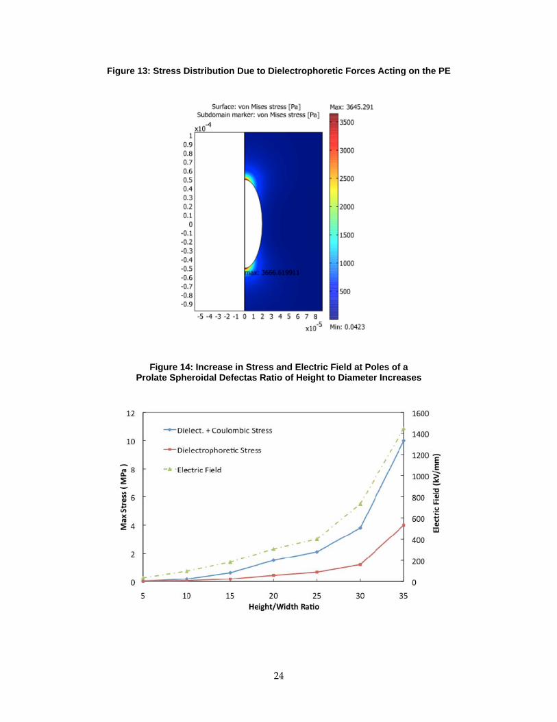
24

Figure 13: Stress Distribution Due to Dielectrophoretic Forces Acting on the PE

Figure 14: Increase in Stress and Electric Field at Poles of a

Prolate Spheroidal Defectas Ratio of Height to Diameter Increases

25

The combination of dielectrophoretic and coulombic stresses at the most extreme aspect ratio studied are likely unrealistic. As the field required to generate these stresses exceeds the dielectric strength of the material, stresses on the order of a few megaPascals are possible before breakdown occurs.

A key point to recognize from the model calculations is that stresses of a few megaPascals should occur within the PE at the ends of long, thin defects. It remains to be determined whether stresses of this magnitude can damage the PE.

2.3.3 The Mechanical Behavior of PE The mechanical properties of various samples of PE insulation were studied using a servo‐hydraulic mechanical testing apparatus (Instron mechanical test system Model 1350). Compression samples were placed between two flat platens and loaded at a displacement rate of 6.858 μm/sec. Loading and unloading tests were run by controlling the displacement of the loading platens while recording the load and displacement. Strain was measured by calculating the ratio of elongation or compression to original sample length, with the assumption that all displacement of the platens was accommodated by deformation of the PE. The inelastic behavior of TR‐XLPE can be seen in

Figure 15 where samples have been unloaded once the strain reaches a predetermined level (0.02, 0.04, and 0.06). The upper curve of each loop shows behavior during loading (platens increasingly squeezing the sample) and the lower curve the behavior during unloading (platens moving apart). The samples are deformed permanently. For example, if the sample is unloaded at a strain of 0.04 (about 7 MPa), it is approximately 1 percent shorter after the test than before.

This inelastic behavior of the PE was found in both used and new samples of PE as shown in Figure 16 (dates indicate year of manufacture) starting at around 3 or 4 MPa. The results of this compression testing suggest that the PE ought to withstand the dielectrophoretic stresses (a few MPa) that would be encountered in service, albeit with some deformation resulting from the stresses. However, the inelastic behavior suggests a different mechanism for mechanical failure, namely fatigue. Fatigue can occur when stresses are applied, then relieved, repeatedly, either in compression or in tension. A related example is found in the paper by Pruitt et al. (1992) on fatigue failure of ultra‐high‐density polyethylene. These researchers studied crack propagation in far‐field compression at up to 2.5 million cycles. Fatigue testing was carried out on TR‐XLPE samples from a new cable sample provided by a commercial manufacturer.

The fatigue testing had to be carried out under conditions different from those anticipated in service:

• Testing was carried out at 5 Hz rather than 120 Hz, because the displacements required to achieve the stress amplitudes of interest in TR‐XLPE cannot be applied at 120 Hz by any mechanical testing apparatus.

• Testing was performed in tension as the compliance of TR‐XLPE allowed the sample to flex in bending without significant stresses being developed. Rigidly fixing both ends of the sample to the machine was necessary for high stress to develop in the sample. Reid

26

et al. (1979) investigated the fatigue mechanism in compression and stated that fatigue crack growth in compression results from residual tensile stresses that arise near a stress concentrator, such as a notch or void. Crack growth in such a situation occurs on the unloading portion of each cycle, in contrast to tensile fatigue where crack growth occurs on loading.

• Experiments were also necessarily shorter than the years or decades of service in the field.

Figure 15: Inelastic Behavior of PE Under Loading and Unloading ofVarious Compressive Strain Levels

27

Figure 16: Inelastic Behavior Exhibited by Six Cable Samples of Various Ages and Chemical Compositions

Further mechanical tests, including fatigue tests, were performed using the geometry prescribed in ASTM D638 ‐ 08 Standard Test Method for Tensile Properties of Plastics (ASTM, 2008); see Figure 17(a). Illustrative examples of samples before and after testing are shown in Figure 17(b). In most cases, the samples fractured during testing (as intended), but in some cases, the samples stretched to the limit of the machine’s extension. These samples, which strained to more than 250 percent of their original length, were said to have failed, because deformation to this magnitude would render the insulation ineffective.

28

Figure 17: PE Mechanical Testing Sample Schematic and Test Samples After Mechanical Testing

(a) Schematic of standard TR-XLPE (b) One untested sample (#15) and

specimen for testing: seven samples after failure. W = 3.18 mm Photo Credit: UC-Berkeley L = 9.53 mm WO = 9.53 mm LO = 63.5 mm G = 7.62 mm D = 25.4 mm R = 12.7 mm

Source: ASTM, (2008)

In order to compare with the results for subsequent fatigue testing, samples were first loaded to failure in monotonic tension. From these data, ultimate tensile strengths were obtained. The ultimate tensile strength is the maximum stress achieved in the material before local plastic instabilities cause localization in deformation. Beyond this point, the engineering stress obtained will apparently decrease, although this is only an artifact of the equation used to define stress (load/original area). Results are seen in Figure 18, where the peak of each stress‐strain curve represents the ultimate tensile strength of that material. The difference in ultimate tensile strengths of XLPE and TR‐XLPE is small, but high density PE (a much stiffer and harder form of PE) exhibits a much higher ultimate tensile strength. The ultimate tensile strength is then used to choose the stress amplitudes (maximum stress minus mean stress) for fatigue testing. As will be discussed below, the maximum stresses applied during the fatigue experiments did not exceed the ultimate tensile strength of the material until the sample was very near to the end of life. As a result, deformation occurred throughout the entire sample. All tests were performed at a load ratio (minimum load/maximum load) of 0.1.

The mechanical responses of XLPE and TR‐XLPE are very similar. However, HDPE, a much stiffer and harder material, can withstand higher stress levels but at the expensive of ductility. XLPE and TR‐XLPE can elongate by more than 150 percent before failure, while HDPE fractures after an elongation of only 75 percent.

Stress amplitudes varying from 3 to 4 MPa, which are well within the range of stresses predicted by numerical analysis of dielectrophoretic forces, were applied to the sample using a

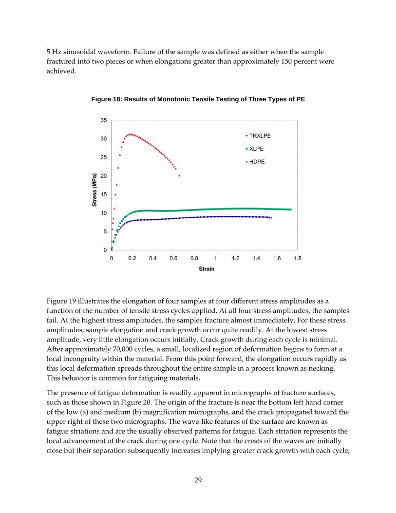
29

5 Hz sinusoidal waveform. Failure of the sample was defined as either when the sample fractured into two pieces or when elongations greater than approximately 150 percent were achieved.

Figure 18: Results of Monotonic Tensile Testing of Three Types of PE

Figure 19 illustrates the elongation of four samples at four different stress amplitudes as a function of the number of tensile stress cycles applied. At all four stress amplitudes, the samples fail. At the highest stress amplitudes, the samples fracture almost immediately. For these stress amplitudes, sample elongation and crack growth occur quite readily. At the lowest stress amplitude, very little elongation occurs initially. Crack growth during each cycle is minimal. After approximately 70,000 cycles, a small, localized region of deformation begins to form at a local incongruity within the material. From this point forward, the elongation occurs rapidly as this local deformation spreads throughout the entire sample in a process known as necking. This behavior is common for fatiguing materials.

The presence of fatigue deformation is readily apparent in micrographs of fracture surfaces, such as those shown in Figure 20. The origin of the fracture is near the bottom left hand corner of the low (a) and medium (b) magnification micrographs, and the crack propagated toward the upper right of these two micrographs. The wave‐like features of the surface are known as fatigue striations and are the usually observed patterns for fatigue. Each striation represents the local advancement of the crack during one cycle. Note that the crests of the waves are initially close but their separation subsequently increases implying greater crack growth with each cycle,

30

consistent with Figure 19. These striations can also be seen in the highest magnification micrographs that were taken from near the fracture origin (Figure 20(c) and (d)).

Figure 19: Elongation of TR-XLPE Samples During Cyclic Loading

Figure 20: Micrographs of Fatigue Fracture at Four Magnifications: Stress Amplitude = 3.25 MPa.

Photo Credits: UC-Berkeley

31

In fatigue studies, a common way of expressing results is with a Stress‐Life plot, also known as a Wöhler or S‐N curve. The number of cycles to failure is plotted on the horizontal axis versus the stress amplitude on the vertical axis. Figure 21 is the measured S‐N curve for TR‐XLPE samples tested at 5 Hz, in air, at a load ratio (minimum stress/maximum stress loading) of 0.1, with the anticipated result that the fatigue life is significantly diminished at higher stress amplitudes. It is emphasized that these measurements are necessarily short‐term compared to the lifetimes of cables. For example, 180,000 cycles is 10 hours at 5 Hz. At the 120 Hz of the dielectrophoretic forces, these cycle numbers are even briefer; for example, 300,000 cycles is reached in 40 minutes. Nevertheless, a large extrapolation from the results of this plot to the lifetimes of a cable yields the following: At 120 Hz, 1010 cycles is equivalent to 2.6 years. Extrapolation suggests that the lifetime would be reached at 1.7 MPa. The stress amplitude required to cause failure after 26 years is, by this extreme extrapolation, 1.6 MPa (0.15 to 3.25 MPa). These are stresses comparable to those predicted by the mathematical model (such as, Figure 14), which implies that fatigue might well be a mechanism for long‐term failure of cable insulation. Also, Sauer et al. (1977) concluded that for polymeric material fatigue where hysteresis losses are significant, an increase of frequency will cause greater energy dissipation. The significant temperature rise may then ensue and deleteriously affect the fatigue lifetime. So for fatigue at higher frequencies, shorter lifetimes are expected for PE.

Figure 21: S-N Curve for TR-XLPE in Air at 5 Hz with a Load Ratio of 0.1

The results of Figure 21 were obtained in fatigue experiments at room temperature—no attempts were made to control the temperature of the samples during testing. It was anticipated that some temperature increase could occur by frictional heating as polymer chains slide past

32

each other (the hysteresis of the loops of Figure 15), but such temperature increase would be small. For example, Sauer et al. (1977) report temperature increases of a degree or two at the stress levels in question for PE. However, to test the TR‐XLPE for susceptibility to failure at higher temperatures that might be encountered in service (such as, from Joule heating in the central conductor or concentric neutrals), samples were enclosed in a heated chamber and further tests run. Figure 22 shows that, for a temperature increase of only 10‐15° C, the cycle life of the TR‐XLPE is diminished by about two orders of magnitude. The maximum and minimum observed life cycles among the six tested samples for each testing condition are shown using the error bars in Figure 22. The effect of temperature reinforces the supposition that fatigue is a credible failure mechanism for cable insulation materials.

The temperature rise in a sample caused by frictional heating during tests performed in air was measured using an infrared surface temperature measurement device: model OS36 IRt/c from OMEGA. Figure 23 shows the results of sample surface temperature measurements during fatiguing of TR‐XLPE samples in room temperature air. The anticipation of a small temperature increase was borne out at low stress amplitude but was not correct for higher stresses. The results are consistent with the temperature increase being due to the mechanical energy input as the sample is taken through the hysteresis loops similar to those seen in Figure 15. The area of the hysteresis loop is the work done on the sample and this area will be larger for higher stress amplitudes because both of the stress and strain are larger. Consequently heat generation within the sample and its temperature are greater at higher stresses.

Figure 22: Diminished Cycle Life of TR-XLPE Samples Tested at Higher Temperature and 3 MPa Stress Amplitude

Error bars designate the maximum and minimum observed life cycles among the tested samples for each testing condition.

33

The temperature increase in the sample can be estimated using the following method. In Figure 15, for example, or a corresponding figure for a cycle in tension, it is possible to calculate the net work done on the sample from the area bounded by each loading curve and its corresponding unloading branch. This can then be expressed as a percentage (about 30 percent) of the work done during loading. If it is assumed that this percentage remains the same during all the fatigue cycles, then the work done on the sample can be calculated for each cycle from the measured extension on that cycle and the imposed stress. This work increases with increasing cycle number as the extension per cycle increases. The calculated results were input into a finite element, steady‐state, heat transfer calculation with a convective heat transfer coefficient at the sample/air interface. The algorithm assumes that 50 percent of the hysteresis energy is converted into heat and the other 50 percent is converted into the breaking of chemical bonds resulting in internal structure change (Rittel and Rabin, 2000). The results of calculations for one stress level appear in Figure 24. Researchers conclude that, on experimental as well as theoretical grounds, the temperature increases due to cycling at the stress amplitudes of interest are small.

In the field, the insulation might experience many more physical effects than elevated temperatures. For example, groundwater or water in conduits or ducts can reach the insulation and common constituents of such water, such as road salt or compounds common in the lithosphere, might also be present. Nikolajevic and Drca (2001) have determined that water reduces the stress on cable insulation, although these authors are referring to the electrical field at which the insulation fails rather than the mechanical stress of interest in the present investigation. Fatigue experiments were therefore conducted with a constant stream of water, delivered from a reservoir to jets impinging on the sample by a pump, flowing over the surface of the sample as shown in Figure 25. This was done for samples not previously exposed to water and for samples that had been kept in water for three months (soaked samples). The temperature of the water was controlled at the sample to 7–8° C above room temperature (room temperatures were 22–23° C), to minimize any cooling offered by the water.

34

Figure 23: Measured Surface Temperature Increases During TR-XLPE Fatigue Testing at Various Stress Amplitudes at Room Temperature

The results are shown in Figure 26, which displays the fatigue lives of both fresh and soaked (for 3 months) samples tested in this water environment. Both soaked samples and samples freshly exposed to water showed enhanced cycle life, even though the temperature was above that of samples tested in air. A hypothesis explaining this unexpected result is that the advancement of a fracture crack through a material is promoted if the newly formed surface reacts chemically with the environment. When fracturing PE in air, the broken bonds will react with oxygen or other corrosive species. If the sample is immersed in water, access to oxygen to the fracture surface is limited and propagation of the fracture slowed. Water may be absorbed at the crack tip causing swelling of the polymer and crack blunting effects similar to what Samat et al. (2009) found with polyvinyl chloride (PVC) in aqueous environments. Further study is necessary to determine the origin of this behavior, although the testing performed here demonstrates that fatigue is still a possible mechanism of failure in service‐like environments.

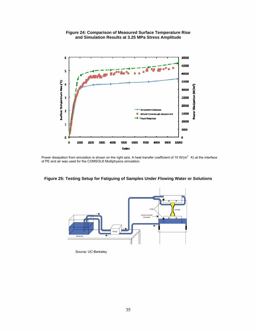
35

Figure 24: Comparison of Measured Surface Temperature Rise and Simulation Results at 3.25 MPa Stress Amplitude

Power dissipation from simulation is shown on the right axis. A heat transfer coefficient of 10 W/(m2�K) at the interface of PE and air was used for the COMSOL® Multiphysics simulation.

Figure 25: Testing Setup for Fatiguing of Samples Under Flowing Water or Solutions

Source: UC-Berkeley

36

Figure 26: Fatigue Behavior of TR-XLPE Samples in Heated Water Environment

Figure 27 shows the results of fatigue measurements in room temperature air, where a sample of TR‐XLPE was first exposed to the sodium salt of humic acid or to acidified ferric chloride solution. Humic acid is a product of the decay of vegetation. The salt was used at a concentration of 1 g/L. The samples were immersed for both three and six months before testing. Although concentration of humic acid used here is higher than that in most groundwater (Delleur, 2007), a high concentration of humic acid was chosen to highlight any deleterious effects and simulate the cumulative effects of prolonged exposure in service. Iron is the fourth most abundant element in the lithosphere (USNY, 2001). Near the Earth’s surface, oxidizing conditions result in much of that iron being present as ferric ions. Also common in the lithosphere are chloride ions. For this reason, fatigue experiments were performed on samples soaked for three months in ferric chloride solution at a concentration of 1 mol/L, also containing 1 mol/L sulfuric acid. Results of these experiments are seen in Figure 27. Both solutions have decreased significantly the fatigue resistance of TR‐XLPE after being immersed. The results of fatiguing samples in flowing, heated humic acid salt solution are displayed in Figure 28 along with the results for humic acid soaked samples tested in air (Figure 27) for comparison. The flowing solution enhances the cyclic life of TR‐XLPE, perhaps by inhibiting oxidation of the forming fracture surface as hypothesized in the previous paragraph. The flow was kept at a constant elevated temperature to mitigate any potential cooling caused by the testing environment.

The micrograph of the fracture surface of a sample that had been soaked in the humic acid salt for three months prior to fatigue in flowing humic acid salt solution is seen at high magnification in Figure 29(a). Compared to the fracture surface shown in Figure 20(d), which is reproduced in Figure 29(b), the sample immersed in humic acid appears to have a much more pitted surface than the one fractured in air, perhaps indicating a greater degree of reaction with the environment in the former case and explaining the results of Figure 28. Also note the flatter

37

surface topography of the fracture surface, indicating a much more brittle fracture for the sample exposed to humic acid.

Figure 27: Fatigue Behavior (in Air) of TR-XLPE After Humic Acid Salt and Ferric Chloride Exposures at 3.25 MPa

Figure 28: Environmental Effects on Fatigue Life of TR-XLPE at a Stress Amplitude of 3.25 MPa

Samples were exposed to 1g/L humic acid salt solutions for various lengths of time. Exposed samples tested in air showed dramatic reductions in fatigue life after only three months of immersion.

38

Figure 29: Fractured Surfaces of Samples Tested


This investigation has been a combination of mathematical modeling for estimating the stresses within the PE and experimentation for determining the mechanical behavior of PE and the effect of various environments on that behavior. The results do not rule against the chemical school , Zeller (1987; 1991) in favor of the electro‐mechanical school. Indeed, the work presented here indicates that they are both correct to some degree; both chemical reactions and mechanical forces, working in concert, are the likely culprits in the development of water trees.

2.3.4 Conclusions The results of this investigation are suggestive, rather than compelling. The application of cyclic mechanical stress is different from the stresses likely experienced by the PE surrounding a water tree in the field. However, the reader will recognize that, in both cases, behavior is determined by material properties, notably the response of the PE to cyclic stress and the environment. The results of the investigation are therefore relevant to propagation of water trees. The conclusions from this investigation are that fatigue of polyethylene insulation due to cyclic dielectrophoretic stresses around defects such as voids or inclusions is a possible mechanism for the development of water trees. Dielectrophoretic stresses can be on the order of a few megaPascals and fatigue experiments in the laboratory suggest that these stresses are sufficient to damage TR‐XLPE insulation in the long term. This suggestion is made more credible due to the experimental results showing that TR‐XLPE is less robust at the higher temperatures likely present in the field. However, there are significant environmental effects. The fatigue life of TR‐XLPE appears to be enhanced in the presence of water but is significantly reduced when TR‐XLPE is exposed to chemical species likely encountered in service.

39

2.4 Charge Injection into Polyethylene: Mechanisms and Experiments 2.4.1 Introduction Charge injection by solid electrodes into insulators is often difficult. The source of the problem is the insulator’s wide band gap and the significant difference in the electron affinity of the insulator and the Fermi level of the metal contact or, in the case of semiconductor contacts, major differences between the electron affinities/ionization potentials of the insulator and semiconductor contacts.

Studies initiated by Kallman and Pope (J. Chem. Phys. 1960, Nature 1960) and continued by others such as Lohmann and Mehl (1975) and Mehl and Hale (1967), indicated that charge injection into organic insulators, like crystals of anthracene, was readily accomplished by using aqueous electrolytes rather than solids as electrodes. Anthracene has a band gap of approximately 5 eV, and the upper edge of anthracene’s valence band could be brought into near coincidence with the energy levels of oxidizing red‐ox couples.

The band structure of polyethylene may be conceptually understood in terms of the progressive changes in the electronic structure of alkanes of increasing number of carbon atoms (Hoffmann et al., 1991). Further details of the electronic structure of polyethylene emerge from considerations of the changes induced in the electronic structure of a chain of carbon atoms by the addition of hydrogen atoms (Hoffmann et al., 1991). This chemical approach indicates that polyethylene should exhibit a very large band gap on the order of 10 eV, which is consistent with the experimentally measured value of 8.8 eV (Less and E. G. Wilson, 1973). Polyethylene’s large band gap and the fact that its electron affinity is negative (Serra et al., 1998) indicate that it is unlikely that charge could be injected into crystalline polyethylene using aqueous electrolytic contacts. However, it might be possible to use electrolytic contacts to inject charge into localized states within the band gap of low‐density polyethylene (LDPE). The electrolytic contacts might facilitate charge injection so that charge is injected at much lower voltages than are necessary when solid electrodes are employed.

There are two motivations for investigating charge injection by aqueous electrolytes into polyethylene. First, as pointed out by Rose (1995) and Smith and Rose (1955), charge injection by solids into insulators provides fundamental information about the insulator’s band structure. Second, from a more practical point of view, charge injection from an aqueous electrolyte could play a role in DC electrical breakdown of polyethylene. Investigating the role of electrolytic contacts might provide insight into the breakdown of polymers employed as high DC voltage insulators as well as water treeing of polyethylene used as high AC voltage insulators.

The present study investigates the injection of charge into LDPE through the use of electrolytic contacts made of aqueous electrolytes containing FeCl3.

2.4.2 Experimental Setup Samples of 25 μm thick LDPE film were prepared from a sheet of LDPE. Samples had dimensions on the order of 30‐40 mm per side. The electrolytic cell used for charge injection is

40

schematically illustrated in Figure 30. The cell consisted of two L‐shaped glass tubes with a flared, circular opening with a circular indentation along the lip. The tubes were approximately 1 cm in diameter with a diameter at the opening of 16 mm. An O‐ring was placed in the indentation of one of the glass tubes, the LDPE sample was place on top of the O‐ring, and then the other glass tube was pressed on to the sample such that the O‐ring and sample were stabilized by the two grooves in the glass tubes. This setup was then clamped, resulting in a watertight seal between the glass tubes and the LDPE sample. The final orientation looks like the letter U, with the open ends of the two L‐shaped glass tubes pointing up and the LDPE sample in the middle, separating the two glass tubes. This then permits different liquid contacts (aqueous electrolytes or Galinstan, a room‐temperature liquid metal alloy) to be added to each L‐shaped glass tube with the LDPE sample being the only electrical contact between the two liquid conductors.

Figure 30: Schematic of Electrolytic Cell Used for Charge Injection

(a) Schematic of the cell (b) Schematic of the electrolyte-polyethylene- electrolyte connection. This U‐shaped apparatus is filled with the liquid electrolytes and placed in a Faraday cage. The electrolytes were connected with platinum wires to a Hypot‐III 3670, which can apply up to 6 kV DC potential between the electrodes. The current was recorded with a Keithley 6485 picoammeter with a 300 MΩ resistor in series to prevent damage to the picoammeter in the event of the breakdown of the polyethylene.

Electrolytes used were air‐saturated 1M H2SO4 with various concentrations of FeCl3: 1M, 0.5M, 0.04M and 0.02M. The control electrolyte was air‐saturated 1M NaCl.

The liquid metal was Galinstan (68.5 at percent Ga, 21.5 at percent In, 10 at percent Sn), a eutectic of gallium, indium, and tin.

Two polarities of cell voltage were used. In forward bias the 1M H2SO4 + FeCl3 electrolyte (referred to as A is at the high potential, with 1M NaCl solution (referred to as B) at ground, and electrochemical reduction taking place on the surface of polyethylene in contact with the A electrolyte. In reverse bias the A electrolyte is at ground with B at the high potential and electrochemical oxidation taking place on the surface of polyethylene in contact with the A electrolyte.

41

For each test, the initial cell voltage was 100 V, then after each 20‐second interval, the voltage was increased by 100 V to a maximum of 6 kV DC, or until 2500 data points had been recorded by the picoammeter. The current was recorded at intervals of 0.31 sec. The tests were also stopped when the current increased to values on the order of the current limits imposed by the 300 MΩ resistor.

2.4.3 Results and Discussion The influence of reverse‐bias voltage across the electrolytic cell on cell current is conceptually presented in Figure 31. Two features of the current‐voltage plots stand out. First, following each 100 V increment in applied cell voltage, the current jumped. At voltages < 2200 V, current density slowly decreases with time and then increases with time at voltages > 2600 V. The current spike and time dependency are responsible for the noisy nature of the data in Figure 31. Second, at a particular value of voltage, equivalent to an electric field in the LDPE of approximately 1 MV/cm, the current density is abruptly raised from a value of a few tens of nA/cm2 to hundreds and thousands of nA/cm2.

Figure 31: Current vs. Voltage for the Electrolytic Cell Under Reverse Bias

Each spike in the current corresponds to a 100 V increment in cell voltage.

In Figure 32, the current density jumped from 60 nA/cm2 to 8,620 nA/cm2 when the voltage was stepped from 4.1 kV to 4.2 kV (approximately 820 sec. after the start of the test). Immediately after the dramatic jump in current, attributed to the LDPE’s breakdown, the applied voltage was decreased to zero. When 100 V was reapplied after breakdown, the current density jumped to 20 nA/cm2. This is orders of magnitude larger than the current density associated with an applied voltage of 100 V before breakdown.

42

A third and fourth feature of importance are the influence of polarity of the cell voltage on the cell current and the non‐linear relationship between cell voltage and cell current. To make clear the relationship between applied voltage and cell current, a section of the data presented in Figure 31 is plotted again in Figure 33 as applied voltage versus cell current at 20 seconds following the voltage increment. The current‐voltage relationship was reproducible as long as the voltage stayed below the value at which the current density abruptly increased to hundreds/thousands of nA/cm2. Note that higher cell currents are generated in reverse bias, that is, when the platinum electrode immersed in the A electrolyte is negatively charged and oxidation occurs at the surface of LDPE immersed in the A electrolyte. In forward bias, that is when the platinum electrode immersed in the A electrolyte is positively charged and low cell currents are recorded.

A test of the electrolytic cell in reverse bias at about 4 kV was run to failure; the cell voltage was reset to 100 V and then stepped 100 V every 20 sec. 200 seconds is equivalent to 1 kV, 400 seconds is equivalent to 2 kV, and so forth. The current density at failure (8.62 x 10‐6 A/cm2) can be seen on this scale.

There are two important observations to be drawn: (1) the effect of voltage on cell current, and (2) the decay of current with time following 100 V steps in cell voltage. These will both be discussed in the remainder of this paper.

Figure 32: Current vs. Time for the Electrolytic Cell Under Reverse Bias

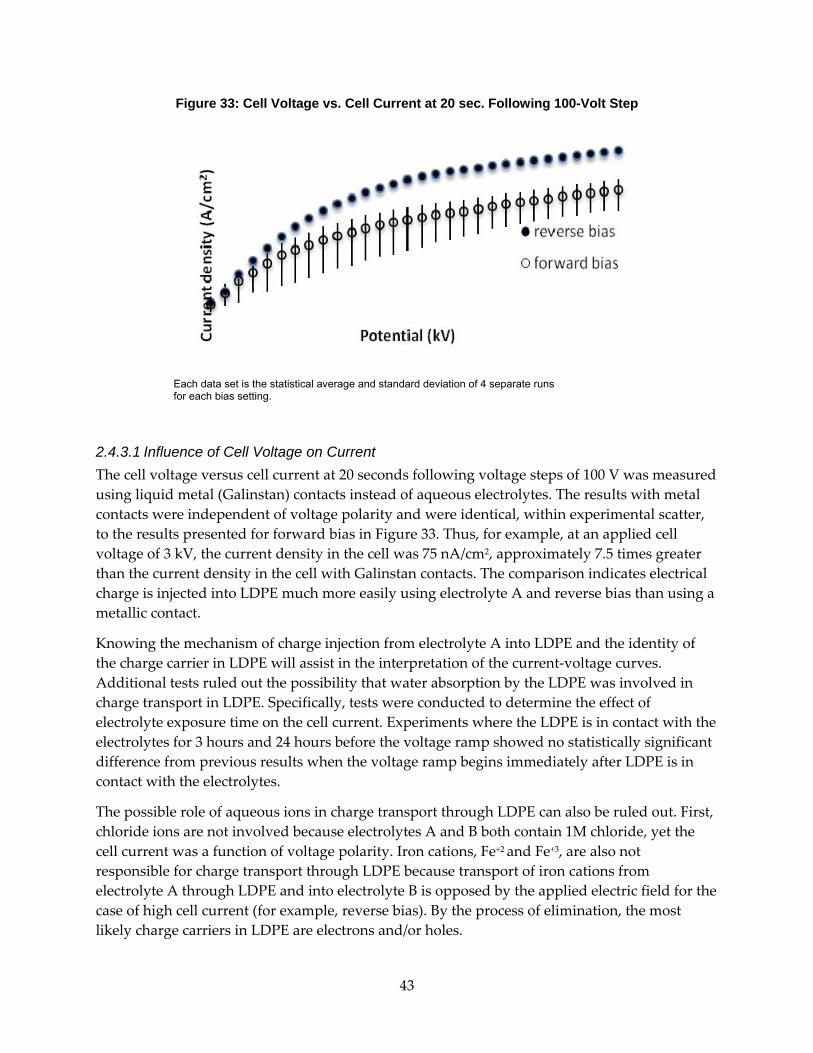
43

Figure 33: Cell Voltage vs. Cell Current at 20 sec. Following 100-Volt Step

Each data set is the statistical average and standard deviation of 4 separate runs for each bias setting.

2.4.3.1 Influence of Cell Voltage on Current The cell voltage versus cell current at 20 seconds following voltage steps of 100 V was measured using liquid metal (Galinstan) contacts instead of aqueous electrolytes. The results with metal contacts were independent of voltage polarity and were identical, within experimental scatter, to the results presented for forward bias in Figure 33. Thus, for example, at an applied cell voltage of 3 kV, the current density in the cell was 75 nA/cm2, approximately 7.5 times greater than the current density in the cell with Galinstan contacts. The comparison indicates electrical charge is injected into LDPE much more easily using electrolyte A and reverse bias than using a metallic contact.

Knowing the mechanism of charge injection from electrolyte A into LDPE and the identity of the charge carrier in LDPE will assist in the interpretation of the current‐voltage curves. Additional tests ruled out the possibility that water absorption by the LDPE was involved in charge transport in LDPE. Specifically, tests were conducted to determine the effect of electrolyte exposure time on the cell current. Experiments where the LDPE is in contact with the electrolytes for 3 hours and 24 hours before the voltage ramp showed no statistically significant difference from previous results when the voltage ramp begins immediately after LDPE is in contact with the electrolytes.

The possible role of aqueous ions in charge transport through LDPE can also be ruled out. First, chloride ions are not involved because electrolytes A and B both contain 1M chloride, yet the cell current was a function of voltage polarity. Iron cations, Fe+2 and Fe+3, are also not responsible for charge transport through LDPE because transport of iron cations from electrolyte A through LDPE and into electrolyte B is opposed by the applied electric field for the case of high cell current (for example, reverse bias). By the process of elimination, the most likely charge carriers in LDPE are electrons and/or holes.

44

Consequently, the direction of cell currents requires electrochemical reactions at the electrolyte/LDPE interface to convert from ionic charge carriers in the electrolyte to electronic charge carriers in the LDPE. In reverse bias, Fe+2 are electrochemically oxidized at the interface and electrons are injected into the LDPE: Feaq+2 Feaq+3 + eLDPE‐. Because the band gap of PE is so large (8.8 eV) the electrons are injected into empty, localized, deep levels in LDPE’s forbidden gap, and not into the conduction or valence bands. The energy of these empty levels must be very close to the energy associated with the equilibrium potential of the Fe+2/Fe+3 red‐ox couple. Consequently, the energy of the empty intragap levels in LDPE that are involved in the oxidation of Fe+2 have an energy of approximately ‐5.27 eV with respect to the zero of energy in vacuum. The ferrous and ferric ions are solvated, so collectively the outer electronic energy levels of the ferrous and ferric ions each form a 1 eV wide band and the mean value of the energies of the two bands is ‐5.27 eV (Morrison, 1980). The density of states corresponding to the occupied level of the ferrous ions is represented by a Gaussian function that spans ≈ ‐5.2 to ‐6.2 eV. For the empty level of the ferric ions is a Gaussian ranging from ≈ ‐4.3 to – 5.3 eV.

During reverse bias, electrochemical reduction must take place at the B/LDPE interface. Possible reducible species in the electrolyte are water (H2O + 2eLDPE‐ ½H2 + OHaq‐) and dissolved oxygen (½O2 + H2O + 2eLDPE‐ 2OHaq‐).

In forward bias, Fe+3 are electrochemically reduced at the LDPE’s surface and holes are injected into occupied deep levels in LDPE: Feaq+3 Feaq+2 + hLDPE+.

It is worth noting that the effect of voltage polarity, in which high cell currents are produced when electrochemical oxidation occurs at the surface of LDPE in contact with the electrolyte that contains a high exchange rate red‐ox couple (such as, Fe+2/Fe+3), is opposite to the influence of voltage polarity when electrolytic contacts were used to inject charge into anthracene. In the case of anthracene, electrons from the electrochemical oxidation reaction were injected into the crystal’s valence band (Kallman and Pope, 1960; Mehl and Hale, 1967). In the present case, as mentioned above, the large band gap of polyethylene suggests that electrons from the electrochemical oxidation reaction are injected into deep levels of LDPE.

The electron exchange rate of the Fe+2/Fe+3 couple is very fast; therefore, concentrations of Fe+3and Fe+2 are approximately equal in the aqueous electrolyte. The higher cell current in reverse bias indicates that the rate of oxidation of Fe+2 at the surface of LDPE is much greater than the rate of reduction of Fe+3 at the LDPE’s surface in forward bias. Since the concentrations of Fe+2 and Fe+3 are identical, the higher rate of oxidation of Fe+2 is attributed to the greater number of empty localized states of energy between ‐4.3 and ‐5.3 eV in the gap compared to the number of occupied localized states of energy between ‐5.2 and ‐6.2 eV in the gap.

To evaluate the role of Fe+2 in the injection of electrons into LDPE, cell current was measured as a function of cell voltage for electrolytes with different concentrations of FeCl3. The results are presented in Figure 34 and summarized in Table 1, which lists the current density flowing through the cell, which is polarized so that electrons are injected from Fe+2 into empty states in LDPE. That is, electrochemical oxidation of Fe+2 occurs at the LDPE/1M H2SO4+xFeCl3 interface.

45

Accordingly, it is expected that the cell current (for example, the rate of charge injection into LDPE) is proportional to the concentration of FeCl3.

Figure 34. Current vs. Voltage for Electrolytic Cell Consisting of 1M H2SO4with 1M, 0.5M, and 0.04M FeCl3

Table 1: Influence of the 1M H2SO4 Electrolyte Cell’s Concentration of FeCl3 on the Cell Current Density in Reverse Bias

The cell current density at 3 kV in 1M FeCl3 is 74 nA/cm2, which suggests that the cell current density in 0.5M, 0.04M and 0.02M FeCl3 should be proportionately lowered to 37, 3, and 1.5 nA/cm2, respectively. The lowest values measured in forward bias and in FeCl3‐free electrolyte are approximately 10 nA/cm2, which suggests that 10 nA/cm2 is attributable to the red‐ox couple present in FeCl3‐free electrolyte, for example, O2/H2O. The cell current density of 26 nA/cm2 measured in 0.5M FeCl3 is in fair agreement with the estimated value of 37 nA/cm2 and is consistent with the proposed mechanism of charge injection from aqueous FeCl3 into LDPE.

Concentration of FeCl3 Current density at

Cell voltage of 3 kV (nA/cm2)

1M

0.5M

0.04M

75

46

The current densities resulting from a cell voltage of 3 kV in 1M H2SO4 with 0.04M and 0.02M FeCl3 are 9 and 8 nA/cm2, respectively, and the current density associated with low concentrations of FeCl3 is much greater than the predicted values of 3 and 1.5 nA/cm2 and is approximately equal to the value of 11 nA/cm2 measured in a solution with no addition of FeCl3. The similar value of current density at 3 kV in 1 H2SO4 with 0 and 0.04M FeCl3 is due to the oxidation of H2O (to ½O2 + 2H+) replacing the oxidation of Fe+2.

Two important parts of the mechanism of current flow in the LDPE that remain to be discussed are the make‐up of the hypothesized extremely deep level in the LDPE into which charge is injected from Fe+2, and the mechanism of charge transport through the LDPE. Information on these two items is provided by measurement of current decay with time.

2.4.3.2 Current Decay with Time The second key observation to analyze is the current decay with time following each 100 V increment in cell voltage. In principle, transport of Fe+2 and Fe+3 in the electrolyte to or from the LDPE surface might be responsible for the current decay following a voltage step, but the following discussion indicates this is unlikely. Specifically, in the case of reverse bias, the electrochemical oxidation reaction on the surface of the LDPE in contact with the Fe+3/Fe+2 electrolyte consumes the oxidizable species, Fe+2, possibly causing the Fe+2 concentration to decrease significantly, which, in turn, would cause the cell current to decrease. However, a significant decrease in concentration of Fe+2 seems unlikely as the rate of oxidation, which is correlated to cell current, is very small and the concentration of Fe+2 is large and equal to the concentration of Fe+3.

Wintle (1974) has identified four processes that result in current decreasing with time following a voltage step applied to an insulator between two electrodes. Two of these mechanisms can immediately be dismissed as possible causes of current decreasing with time following a 100 V step applied to LDPE between aqueous electrodes. The first mechanism, dipolar relaxation (Cole and Cole, 1942; Neagu et al., 2000) which occurs entirely within the insulator and is therefore independent of the electrode materials, is contrary to the results that indicate an important role of the electrodes. The second process that can be dismissed is termed polarization (Beaumont and Jaco, 1967; Tiebensky and Wintle, 1972; Kahn and Maycock, 1967; Macdonald, 1971). Polarization results from a build‐up of charge in the insulator close to the insulator/electrode interface as a consequence of a fast rate of carrier transport through the insulator relative to the rate of carrier discharge at blocking or partially blocking electrodes. The polarization effect is generally ascribed to ionic insulators. Polarization is an unlikely cause of absorption current in LDPE because: (1) the presence of a significant concentration of mobile carriers in LDPE is unlikely given the large band gap of LDPE, and (2) any charge carriers in deep localized intragap states are likely to have very low mobility.

To Wintle’s four processes, Das Gupta and Brockley (1978) added a fifth that is based on charge carrier hopping in the insulator (Wintle, 2003; Romanets and K. Yoshino, 2004), which can be dismissed from consideration. Charge carrier hopping through LDPE is not likely the cause of the absorption current in researchers’ experiments because the results depend on the identity of the electrodes.

47

The two remaining methods by which a voltage step can cause a decreasing current versus time are tunneling (Wintle, 1973) from the electrode to empty states in LDPE and charge injection from the electrode leading to space charge effects in LDPE (O’Dwyer, 1966; Lengyel, 1966; Lilly and J.R. McDowell, 1968; Lilly et al., 1968; Taylor and Lewis, 1971). Both of these mechanisms are consistent with the experimental results that indicate the important role of the electrodes. Tunneling and charge injection/space charge effects require the presence of electrodes with Fermi levels aligned with levels of the insulator.

Because PE has a large band gap and small electron affinity, the Fermi Level of the aqueous solution with 1M FeCl3, which has energy of ‐5.7 eV, is very deep within PE’s forbidden gap. Results of earlier studies of PE have suggested the presence of deep levels but have not shown any direct evidence of deep levels (Wintle, 1974; Huzayyin et al., 2008). Calculations (Meunier and Quirke, 2000) indicate the highest probable energies for additional energy levels inside the bandgap of PE are nowhere close to the Fermi level of aqueous 1M FeCl3 (Meunier and Quirke, 2000; 2001; Teyssedre, 2001). Specifically, physical defects in PE provide shallow levels with depths below the conduction band of < 0.5 eV (Meunier and Quirke, 2000). Chemical defects associated with cross‐linking agents provide levels with calculated depths less than 2 eV (Meunier and Quirke, 2001; Anta, 2002).

Of course, even if extremely deep levels (for example, absolute energies in the range of ‐4.3 to ‐5.3 eV) were present in the bulk of LDPE, it is unlikely that they would contribute significantly to carrier transport. The mobility of electrons injected into extremely deep levels would be far too small at room temperature.

To account for the discrepancy between experimental results that suggest the presence of deep levels and the failure to detect deep levels, some investigators have proposed that deep levels are present at the insulator’s surface, which enables charge injection, but that the deep levels are not found within the insulator’s bulk, which explains the inability to directly detect deep levels Wintle (1974).

The experimental results of Suzuoki et al. (1984) and Mizutani et al. (1983) confirm that deep levels on the surface of insulators do enhance charge injection. Doping the surface of PE with acetoxy groups and hydroxyl groups (Suzuoki et al., 1984) introduced deep levels and enhanced the rate of charge injection from metal electrodes. Although present throughout the bulk and not confined to the surface, an antistatic agent enhanced the rate of charge injection into HDPE by introducing deep levels (Mizutani et al., 1983) as well as forming a hetero surface space charge (Suzuoki et al., 1985). It is also worth noting that surface oxidation (Mizutani, and Ieda, 1979; Mizutani et al., 1980) of HDPE introduces deep levels, such as those associated with carbonyl groups (Huzayyin et al., 2008) that might contribute to charge injection.

The key role of surface levels in the injection of charge into LDPE by aqueous 1M FeCl3 is supported by the results of the experiments in which the current immediately decreased and changed polarity (and finally, rapidly decayed to zero) when the applied voltage was abruptly turned off. Charge injection into deep levels in the bulk of an insulator resulted in current that

48

did not change polarity when the voltage was stepped to zero. The discharge current was a consequence of the slow emptying of deep bulk levels (Romanets and Yoshino, 2004).

A combination of surface states or extremely deep levels confined to the near‐surface region along with a mechanism of mobile charge carrier formation described by Lewis can explain the effective charge injection by aqueous 1M FeCl3 (Lewis, 2002). According to this mechanism, electrons from Fe+2 are injected into extremely deep surface traps with energies between ≈ ‐5.2 and ‐6.2 eV. The electrons then drop into valence band holes, which are brought to the LDPE’s surface by the applied voltage during reverse bias. Energy conservation is satisfied by Auger processes that couple the annihilation of a hole (which releases an energy of 2.6 to 3.6 eV for a valence band edge located at ‐8.8 eV) with, for example, the excitation of another electron from Fe+2 to an energy of ‐2.6 eV, which might coincide with a shallow trap. This mechanism would attribute the unique role of the Fe+2/Fe+3 red‐ox couple to the specific value of its equilibrium potential (for example, Fermi Level) and the rapid electron exchange between Fe+2 and Fe+3.

To further explore the proposed mechanism, future experiments will investigate the effect of temperature (as a way to distinguish between tunneling of electrons and other mechanisms of charge injection), the composition of the aqueous electrolyte (to probe the effect of the solution’s Fermi Level), and the type of PE (XLPE, HDPE, and so forth) as well as the performance of other polymeric insulators (to determine the influence of surface states and very deep traps).

2.4.4 Conclusions Electrical charge from aqueous electrolytes of 1M H2SO4 + 0.5M and 1M FeCl3 were injected into LDPE under the influence of high applied voltage. The amount of charge injection decreases as the concentration of Feaq+2 decreases. The charge injected by the aqueous FeCl3 solutions is significantly greater than the charge injected by aqueous 1M NaCl and by liquid metal (Galinstan) contacts. The influence of voltage polarity and electrolyte composition on plots of current versus voltage, and the decrease of current with time following voltage steps of 100 V suggest charge injection consists of oxidation of Feaq+2 at the surface of the LDPE and the transfer of electrons into LDPE.

The plots of current versus voltage and the decay of current with time are consistent with a mechanism of charge injection from metal conductors into insulators (Lewis, 2002). Specifically, electrons from the oxidation of Feaq+2 are injected into empty, localized, deep surface levels in LDPE. Based on the range of electronic energies of aqueous ferrous ions, the energies of the hypothesized deep surface levels are ≈ ‐5.2 to ‐6.2 eV. Charge transport through the LDPE occurs by electrons in the surface states annihilating valence band holes and Auger excitation of coupled surface state electrons to shallow states below the LDPE’s conduction band.

The results demonstrate that charge injection from aqueous electrolyte contacts into an insulator provides the energies of some localized intragap states of LDPE. From a more practical point of view, the present results indicate that charge injection by an electrolyte might contribute to electrical breakdown of high voltage DC insulators. Researchers are presently investigating charge injection into polyethylene from electrolytic contacts under the influence of high AC voltage.

49

CHAPTER 3: Online Methods for Probing the Integrity of Insulation in Underground Power Distribution Cables 3.1 Introduction In this section researchers describe the research on developing online diagnostic methods and sensors for probing the integrity of the insulation in underground power distribution cables. Specifically, researchers present two techniques: the Interdigitated Dielectrometry which probes the condition of the insulation below the actual sensor location, and the radio frequency (RF) Test‐point Injection Probing, which probes the insulation in the cable remotely (from within the locations of the vault) by injecting an RF test‐pulse into the cable through the elbow test‐points.

3.2 Interdigitated Dielectrometry 3.2.1 Introduction Interdigitated dielectrometry (ID) consists of a set of interdigitated electrodes that project an AC electric field through the PE insulation. Changes to how the electric field penetrates the insulation and is picked up by the opposing set of electrodes can indicate changes in the permittivity due to water trees.

3.2.2 Theory The sensors utilize the fact that different materials have different relative permittivity, or dielectric constants εr, which describes how well electric fields penetrate the material. The constituents of each material determine its dielectric constant. Physical changes, such as degradation, in the material cause a change in its dielectric property.

Figure 35 shows the geometry (left) and the equivalent circuit diagram (right) of an ID sensor. The sensor consists of the driving electrode and the sensing electrode. The electrodes are placed on top of an insulating substrate. A sinusoidal potential is applied to the driving electrode, and the output is read at the sensing potential.

Figure 35: The Geometry and Equivalent Circuit Diagram of an ID Sensor

50

The important features of the capacitor are its electrode width, w, its gap width between the electrodes, g, the electrode finger length, L, and the number of fingers, N, the sensor has. Vin is the driving potential and Vout is the sensing potential.

In order to detect insulation degradation, most of the electric fields emanating from the sensor must be concentrated in the material under test. Without a conducting backplane, the electric fields will travel through the substrate and greatly influence the capacitance readout; although researchers can account for the effect of the substrate alone, it is generally difficult to do so. To facilitate calculation, researchers add a conducting (copper) backplane. Because electric fields do not exist within a conductor, the backplane will cut off any electric fields emanating from the back of the sensor. Although the substrate will still affect the capacitance of the sensor, by applying the driving potential to the backplane, it is much easier to calculate the effect of the substrate on the total capacitance.

Figure 36: Electric Field from an ID Sensor Passing Through a Void in the Insulation.

Under operation, the sensor may be attached to the insulation. If water trees or voids form inside the insulation, the effective dielectric property of the insulation will deviate from that of a healthy insulator. As a result, the capacitance of the sensor will change. Researchers can approximate the change in capacitance. From Figure 36, let l be the average length of the field lines of the electric field above the sensor. Then let lm and lv be the average length of the field lines passing through the material and void, respectively. Then, because the dielectric slabs of the materials on top of the capacitor is in series, the effective dielectric constant is:

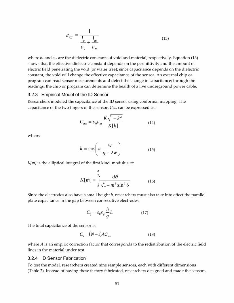
51

m

m

v

veff ll

εε

ε+

=1

(13)

where εv and εm are the dielectric constants of void and material, respectively. Equation (13) shows that the effective dielectric constant depends on the permittivity and the amount of electric field penetrating the void (or water tree); since capacitance depends on the dielectric constant, the void will change the effective capacitance of the sensor. An external chip or program can read sensor measurements and detect the change in capacitance; through the readings, the chip or program can determine the health of a live underground power cable.

3.2.3 Empirical Model of the ID Sensor Researchers modeled the capacitance of the ID sensor using conformal mapping. The capacitance of the two fingers of the sensor, Cms, can be expressed as:

][1 2

0 kKkKC mms

−= εε

(14)

where:

⎟⎟⎠

⎞⎜⎜⎝

⎛+

=wg

wk2

cos π

(15)

K[m] is the elliptical integral of the first kind, modulus m:

∫ −=

2

022 sin1

][

π

θθ

mdmK

(16)

Since the electrodes also have a small height h, researchers must also take into effect the parallel plate capacitance in the gap between consecutive electrodes:

LghC gg εε0=

(17)

The total capacitance of the sensor is:

( ) mss ACNC 1−= (18)

where A is an empiric correction factor that corresponds to the redistribution of the electric field lines in the material under test.

3.2.4 ID Sensor Fabrication To test the model, researchers created nine sample sensors, each with different dimensions (Table 2). Instead of having these factory fabricated, researchers designed and made the sensors

52

ourselves. First, researchers created the images of each sensor with computer‐aided design (CAD) software such as AutoCAD. After designing the sensors, researchers printed them on glossy photo paper with a laser jet printer. Researchers then took the printed design, mounted the paper faced down on polyimide double‐sided copper plates, and ironed the image onto the copper plates. Note that glossy photo paper and a laser printer are both required; the laser printer applies the toner that is necessary for the sensor fabrication and glossy photo paper facilitates the transfer of toner onto the copper plates. After ironing for twenty minutes, researchers removed the paper with hot water and were left with copper plate with the capacitor design images printed on them. Then researchers taped the side opposite the image for the backplane and placed the copper plates into a solution of ferric chloride. The toner and tape inhibits the reaction of ferric chloride with copper, so once the solution etched away the unnecessary copper, researchers were left with the final product (Figure 37).

Table 2: Dimensions of the Fabricated ID Sensors

Figure 37: A Fabricated Interdigitated (ID) Sensor

Photo Credit: UC-Berkeley

53

3.2.5 Experimental Results The capacitance of the fabricated ID sensors was recorder as the sensors were exposed to materials with different dielectric properties. Table 3 shows the resulting capacitance when the fields from the nine ID sensors pass through air, XLPE, and a book cover.

Although the ID sensor can discern the dielectric constants of different materials, it uses the electric field, which can potentially be shorted by the conductive semicon layer. Figure 38 shows the cross‐section drawing (left) and the equivalent circuit diagram (right) of the ID sensor attached to the outside of the underground power distribution cable, respectively.

Table 3: Recorder Capacitance of the ID Sensor Subject to Various Materials

Figure 38: Cross-section and Equivalent Circuit Diagram of ID Sensor

In order to reach the insulation, the electric field has to travel through the semiconductive layer, called semicon, which is used to smooth out the electric field between the CNs and the CC. By analyzing the circuit in Figure 38, researchers have discovered that the field is largely shorted, and does not significantly enter the insulation layer. Figure 39 shows the impedance of the

54

various layers in the cable, corresponding to the layers on Figure 38. Note that the impedance of the semicon layer (Zs) is 8 orders of magnitude smaller than the impedance of any of the other layers. This indicates that any electric field attempting to pass through the semicon layer will be largely shorted.

3.2.6 Conclusions Researchers have developed the ID technique and adopted it for making measurements to detect the degradation of the insulation in underground power distribution cables. Researchers have shown that researchers can fabricate ID sensors capable of probing the dielectric constant of different materials. However, researchers have found that the semiconductive layer called semicon effectively shorts the field emanating from the ID sensors, limiting their applicability as an online diagnostic method for underground power distribution cables.

Figure 39: Impedance of the Various Layers of Cable Insulation at Different Frequencies

Source: UC-Berkeley

3.3 RF Test-point Injection Probing 3.3.1 Introduction It is well known to the power utilities that imperfections known as water trees can develop in the insulation of power distribution cables. Starting from imperfections (micron‐sized voids) in the cable insulation, the imperfections may grow due to electromechanical or chemical forces

55

(Maxwell stresses) until they ultimately cause a destructive arc discharge in the insulation that renders the cable unusable. As the water trees grow, they affect the permittivity and conductivity of a cable’s insulation, causing changes that might be helpful in detecting badly water‐treed cable that should be replaced to avoid explosive failures. But replacement must be done selectively, since cable replacement is very expensive, estimated at no less than $100,000/km for cable replacement in an urban area (Werelius et al., 2001).

One of the main goals of this research was to evaluate novel techniques for detecting water trees in energized underground power distribution cables, for use in condition‐based cable replacement methodologies.

In what follows, researchers describe ways of introducing RF probing signals into a functioning energized cable by using the test points found on the elbows used at both ends of underground cable conduits. Researchers will describe the generally accepted water tree characteristics, the possible use of the cable test points for cable probing, and the auxiliary equipment needed for such testing. Researchers will also describe the processes and difficulties of obtaining water trees for experimental study, and methods for measuring both RF signal loss and phase velocity of propagation in cables designed for power distribution at 10 to 60 kV and 50 Hz or 60 Hz. Lastly, researchers will describe the initial probing tests and modeling performed.

The Morphology of Water Trees The description of water trees (Figure 40) proposed by Hvidsten and Ilstad (1998) is now widely accepted (such as, see Dubickas and Edin (2008)).

Figure 40: Magnified View of Cable Insulation Showing Void and Water Tree Formation

Source: Hvidsten and Ilstad (1998)

56

Water trees often begin as micron‐sized imperfections, such as voids or bits of contamination in the insulating polymer of the coaxial cables. Owing to the presence of strong electric fields in the insulation, the associated Maxwell stresses produced in the coaxial cable’s insulator may gradually tear apart the insulation creating nanometer‐sized channels that connect nearby voids. These hydrophilic structures fill with water in which the cables are often immersed. These water‐filled structures, the voids and the channels between them, increase both the dielectric permittivity and the electrical conductivity locally in the insulation, thus increasing the capacitance and lowering the resistance per unit length of the cable. These changes will lower the phase velocity of electromagnetic waves propagating in the cable, and will increase the loss incurred by such propagating waves in the cable (Figure 41). Quoting from Dubickas and Edin (2008), The dielectric properties of the power cables with water trees are voltage dependent (Werelius et al., 2001) and show an increase in the capacitance and the loss with the increase of the applied high voltage. Werelius et al. (2001) have also commented on the possibility of using harmonic generation diagnostically in view of the nonlinearity of the water tree behavior (see also Thomas and Saha (2008) regarding nonlinear effects). In addition to being voltage dependent, the effects upon the permittivity and the conductivity of the cable insulator depend on the frequency of the high voltage that acts upon the trees (Dubickas and Edin, 2008).

Figure 41: Permittivity and Conductivity of Water-treed Cables

Source: Hvidsten and Ilstad (1998)

57

In a comprehensive article, Ross (1998) further describes the properties of water trees as follows:

Water trees are degradation structures in a polymer that:

1. Are permanent,

2. Have grown due to at least humidity and an electric field,

3. Have a lower electrical strength than the original polymer when wet, but which are not a short circuit or local breakdown path, and

4. Are substantially more hydrophilic than the original polymer.

3.3.2 Proposed Measurement Technique Researchers propose the following on‐line technique for evaluating the degree of water‐treeing in energized power distribution cables:

a. Measure the propagation characteristics (velocity of propagation and attenuation) of a RF probing signal introduced into the cable that is also energized by its usual low‐frequency 50 Hz or 60 Hz AC voltage.

b. Observe the RF transmission characteristics of the cable in synchrony with the AC voltage.

c. Compare the RF phase velocity and/or the RF loss at times during at least one‐quarter of an AC cycle as the applied AC voltage varies from zero (zero‐crossing value) up to its maximum (peak) value. Figure 42 shows schematically one‐half cycle of the high‐voltage AC and the times at which RF measurements of loss and phase velocity would be made.

d. Severe water‐treeing would be indicated by decreased RF phase velocity and/or increased RF loss at the time when the applied AC voltage is at its peak compared with those quantities when the applied AC voltage is crossing zero.

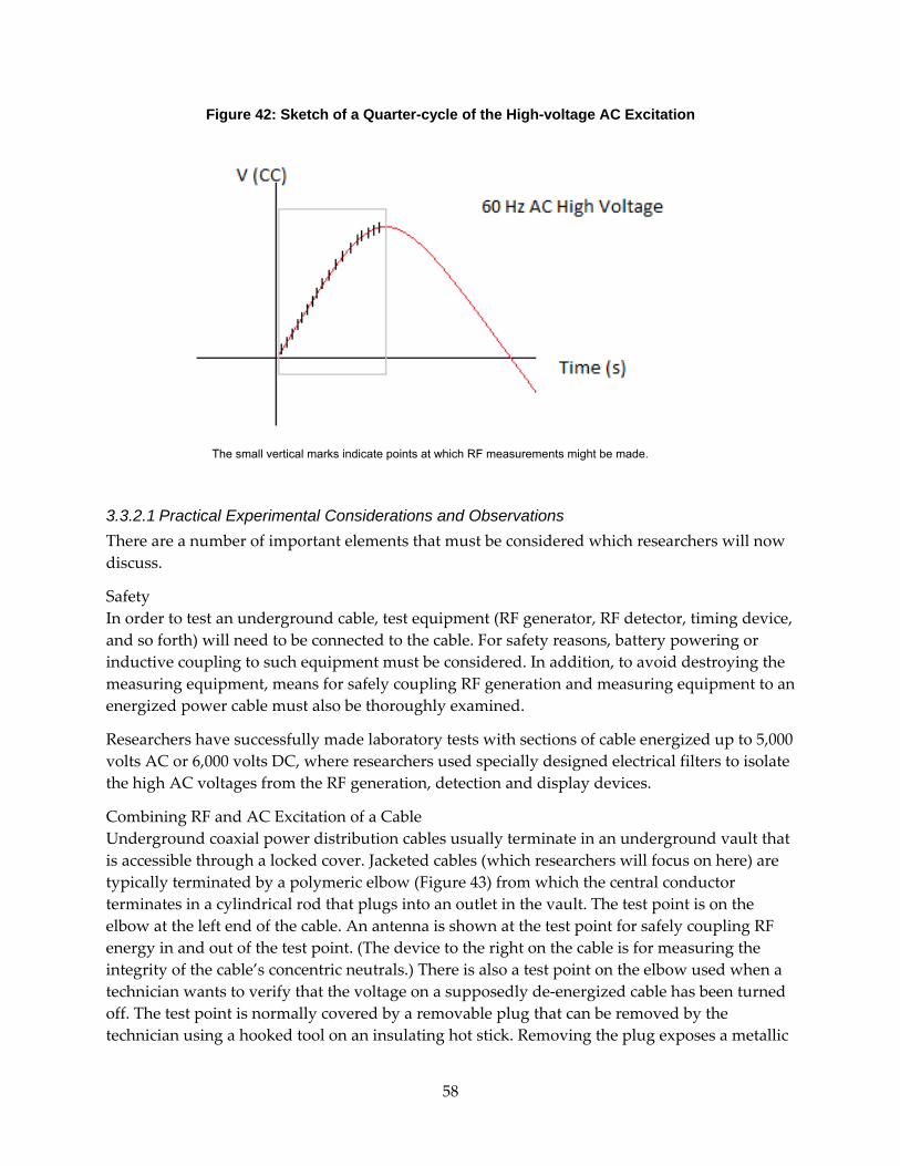
58

Figure 42: Sketch of a Quarter-cycle of the High-voltage AC Excitation

The small vertical marks indicate points at which RF measurements might be made.

3.3.2.1 Practical Experimental Considerations and Observations There are a number of important elements that must be considered which researchers will now discuss.

Safety In order to test an underground cable, test equipment (RF generator, RF detector, timing device, and so forth) will need to be connected to the cable. For safety reasons, battery powering or inductive coupling to such equipment must be considered. In addition, to avoid destroying the measuring equipment, means for safely coupling RF generation and measuring equipment to an energized power cable must also be thoroughly examined.

Researchers have successfully made laboratory tests with sections of cable energized up to 5,000 volts AC or 6,000 volts DC, where researchers used specially designed electrical filters to isolate the high AC voltages from the RF generation, detection and display devices.

Combining RF and AC Excitation of a Cable Underground coaxial power distribution cables usually terminate in an underground vault that is accessible through a locked cover. Jacketed cables (which researchers will focus on here) are typically terminated by a polymeric elbow (Figure 43) from which the central conductor terminates in a cylindrical rod that plugs into an outlet in the vault. The test point is on the elbow at the left end of the cable. An antenna is shown at the test point for safely coupling RF energy in and out of the test point. (The device to the right on the cable is for measuring the integrity of the cable’s concentric neutrals.) There is also a test point on the elbow used when a technician wants to verify that the voltage on a supposedly de‐energized cable has been turned off. The test point is normally covered by a removable plug that can be removed by the technician using a hooked tool on an insulating hot stick. Removing the plug exposes a metallic

59

conductor that is connected via a small‐valued (such as, 32 pF) capacitor connected to the central conductor (CC). Researchers propose to couple the RF probing signal into the CC via the capacitor. Filters that researchers would use in fields tests to prevent the high AC voltage from destroying the RF equipment were successfully used in the laboratory tests at voltage (they replaced the capacitors labeled CTP seen in Figure 44).

Figure 43: View of the Elbow on a Jacketed Power Cable

Source: SolidWorks™

In addition or alternatively, researchers may employ inductive means to couple RF signal into and out of test points on the elbows.

To keep the high voltage from the RF generation and display devices in the laboratory tests, researchers used high‐pass filters between the RF source and the 32 pF capacitors that represented the test point capacitors. (In field tests researchers would also use such filters between the RF components and the cable test points.)

One‐ended Detection vs. Two‐ended Detection RF probing can be done one‐ended or two‐ended. For one‐ended detection, researchers launch the RF probing signal at one end of the cable causing the RF wave to propagate to the far end of the cable where it will be reflected because of the impedance mismatch there. The reflected RF wave will propagate back to the launch point where it can be detected and analyzed. A field‐ready portable sophisticated electronic device, a network analyzer, connected via the test point at the launch end both generates a frequency‐swept RF signal and compares it with the return signal reflected from the far end of the cable. The network analyzer (NI FieldFox) outputs or stores the amplitude ratio of the reflected to transmitted RF signal for analysis to determine the attenuation due to the two transits of the energized cable. Researchers have observed that researchers can also determine the RF phase velocity of the cable by analyzing resonances owing to reflections at the ends of the cable (Figure 45).

60

Figure 44: Schematic of Model of Cable with AC and RF Feeds

Figure 45: Network Analyzer Display of Ratio of Reflected RF Signal to Transmitted Signal for a 100-foot Un-energized Cable

The peaks observed are uniformly spaced in frequency and result from resonances of the RF waves propagating in the cable for which the ends represent reflective impedance mismatches.

For two‐ended detection (Figure 46), researchers would couple to the test points at both ends of the cable, launch an RF wave from one end and measure its amplitude at the second end to find

61

the attenuation due to one transit of the cable. For this test, a spectrum analyzer can be used as a narrowband RF detector. Determining the RF phase velocity from the signal at the far end may be possible using a procedure analogous to the resonant scheme described above.

Figure 46: Two-ended Cable Test Setup Utilizing the Test Points to Launch and Receive the RF Probing Signals

Utilities may prefer one‐ended testing because it involves operating within a single vault.

Measuring RF Phase Velocity The resonant behavior of the cable shown in Figure 45 can be used to determine the RF phase velocity in the cable as the AC excitation goes through one‐quarter cycle (or through many cycles in which RF measurements are made at slightly different times in each successive cycle, which is the operating principle of the sampling oscilloscope). If the phase velocity decreased as cable capacitance rose, the frequency differences between resonant peaks would change.

Note: Researchers attempted to measure phase velocity with the conventional time‐domain reflectometer while coupling to the cable through a test point but were unable to obtain a usable indication (we used a Riser Bond Model 1205CXA Coaxial Metallic Time Domain Reflectometer kindly provided by PG&E).

Obtaining Water‐treed Cables for Study Since the beginning of this research project researchers have attempted to obtain samples of test cables known to contain water trees. To date researchers have obtained such samples with confirmed water treeing. Researchers have taken two approaches to obtain cable samples. The first approach was to obtain samples thought to contain water trees from the utilities. However, visual tests on samples received (samples were dyed with methylene blue, or, alternatively, heating a smooth section in silicone oil and looking for brush like discolorations) have failed to

62

show water trees. Secondly, researchers employed a technique from the literature (Givens et al., 2001) to grow trees in un‐aged cable. The technique involved submerging cable with exposed insulation in a 0.1 M NaCl solution and applying a high AC voltage (5,000 volts) for about 2 months (Figure 47). Researchers were unable to perform a challenging 250o C thermal discharge test after treating the cable. Researchers did test that cable section, in which water trees may or may not have grown, but the 5,000‐volt test did not show evidence of response to water trees.

Figure 47: View of the Polymeric Non-conducting Container


3.3.3 Modeling RF Propagation in a Water-treed Cable Researchers have modeled, with the circuit analysis application LT‐Spice, the anticipated effects of the changes of permittivity and conductivity of the insulator in a water‐treed cable. The circuit model is shown in Figure 44. Figure 48 and Figure 49 show the calculated effects of changes of the relative permittivity and the conductivity of the insulation in a 100‐foot cable where water trees are present, respectively. The estimated permittivity and conductivity values are from Toyoda et al. (2001) who made space charge distribution measurements on water trees in polyethylene. These plots suggest that the growth of water trees will indeed produce changes in the attenuation of RF probing signals in a water‐treed cable. Of course, the magnitude of the effects caused by water trees must depend on the density and size of the water trees in the cable under test (one source referred to the occurrence of a high density (at least 106 per cubic millimeter) of water‐filled voids. Researchers also expect that the length of the trees will be an important factor in determining their detectability, with the longest trees most likely leading to breakdown (Ross, 1998).

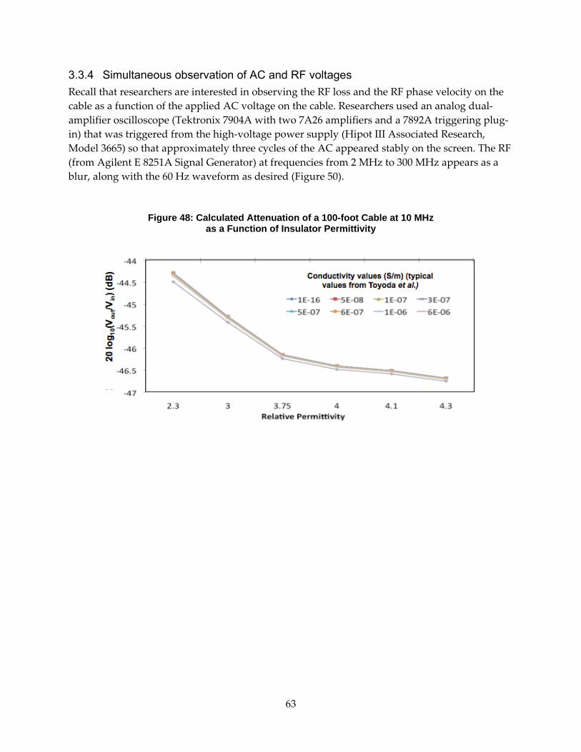
63

3.3.4 Simultaneous observation of AC and RF voltages Recall that researchers are interested in observing the RF loss and the RF phase velocity on the cable as a function of the applied AC voltage on the cable. Researchers used an analog dual‐amplifier oscilloscope (Tektronix 7904A with two 7A26 amplifiers and a 7892A triggering plug‐in) that was triggered from the high‐voltage power supply (Hipot III Associated Research, Model 3665) so that approximately three cycles of the AC appeared stably on the screen. The RF (from Agilent E 8251A Signal Generator) at frequencies from 2 MHz to 300 MHz appears as a blur, along with the 60 Hz waveform as desired (Figure 50).

Figure 48: Calculated Attenuation of a 100-foot Cable at 10 MHz as a Function of Insulator Permittivity

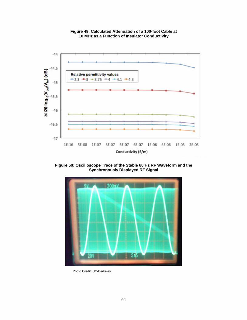
64

Figure 49: Calculated Attenuation of a 100-foot Cable at 10 MHz as a Function of Insulator Conductivity

Figure 50: Oscilloscope Trace of the Stable 60 Hz RF Waveform and the

Synchronously Displayed RF Signal


65

3.3.5 Conclusions Researchers tested a 1.4 m length of un‐aged cable and a 1 m length of treated cable at various frequencies. Even though the XLPE cables tested were designed for higher AC voltages than researchers could generate in the lab, and researchers had no evidence that the treated cable actually contained water trees, these tests did resolve a number of issues:

1. Researchers demonstrated the ability to make RF measurements on energized cables via the cable test points.

2. Researchers safely made RF measurements on energized cables in the laboratory with no equipment failures due to electrical breakdown.

3. Researchers showed that researchers can make cable measurements at RF frequencies in the range from 2 MHz to 6 GHz by using, in some instances, a portable (Agilent) network analyzer and spectrum analyzer, designed for convenient field use.

4. Researchers showed that the measurements with a network analyzer can be made via the test points in the available cable elbows.

5. Researchers were able to obtain a synchronized display of the AC excitation and the RF probing signal to compare the RF behavior at varying points in a quarter‐cycle of the energizing AC voltage.

6. Researchers discovered a way to infer the RF phase velocity from RF probing via the cable test points.

7. Researchers experimented with a technique from the literature for artificially aging a cable to grow water trees.

8. Researchers carried out modeling of a water‐treed cable using an analytic approach and a simulation approach using LTSpice, based on expected values of the permittivity and conductivity of the polymeric cable insulation with and without water trees.

66

CHAPTER 4: Online Methods for Probing the Integrity of Concentric Neutrals in Underground Power Distribution Cables 4.1 Introduction Researchers proposed and investigated two methods for probing the integrity of the CNs in U/G power distribution cables: Surface‐guided RF wave (Goubau) probing and Magnetic CN or amorphous magneto‐resistive (AMR) probing. Both methods can be applied to energized cables without the need of de‐energizing the cable or disconnecting the cable form the grid.

4.2 Surface-guided RF wave (Goubau) Probing 4.2.1 Introduction Surface‐guided RF wave (Goubau) probing uses the concept of a surface‐guided RF wave to probe for breaks in the CNs. The surface‐guided waves were originally proposed by George Goubau (Goubau, 1950) and are referred to as Goubau Waves (GW). The GW is launched along the cable using a conical launching device (funnel) and non‐invasive capacitive coupling to the CNs, allowing the cable to remain energized while the test is being performed. The GW is guided along the cable, and any discontinuities, breaks, or corrosion in the CNs will reflect and attenuate the signal transmitted to a neighboring vault.

4.2.2 Experimental Setup The GW experiments were conducted on three setups: 1) single‐wire transmission line (in‐lab), 2) elevated underground power distribution cable (in‐lab), and 3) partially placed on the ground power distribution cable (outdoors). In all experiments, the RF‐signal was generated using an Agilent E8251A programmable signal generator, and modulated with a pulse from an Agilent 33220A arbitrary function generator. A 4‐channel 2GHz digital oscilloscope (Agilent Infinium DSO80204B) was used to register both the transmitted and received signals. The power of the received signal was also recorded using the Agilent 8562EC spectrum analyzer.

Setup 1: Thirty feet of single insulated braided copper wire (Ø 4 mm) was suspended one foot below the ceiling to facilitate unobstructed transmission of the GW. A photograph of this setup is shown in Figure 51 at left, showing the launch and receive cones and the transmitting wire; a schematic of the setup is shown on the right. The signal was coupled galavanically at both ends to the central conductor.

Setup 2: The signal was capacitively coupled to CNs in a 90 feet section of a 1 10 CN jacketed TR‐XLPE cable (ICC Brand‐MTT, #2 Solid Al, 175 Mils TR‐XLPE 15 kV, Insulating PF Jacket). The cable was elevated on ten 29‐inch tall plastic traffic cones to avoid the interaction of the wave with the reinforced concrete floor underneath. The launching and receiving funnels were made of 5‐mil thick soft copper foil with an outer diameter of 11.5 inches and an inner diameter of 2 inches. The funnels were attached to 11.5‐inch long coaxial sleeves, which were meant to encourage the transition from TEM to TM mode. The cable looped around the room; the

67

transmitting and receiving funnels were separated by approximately 6 feet. A photograph of this setup is shown in Figure 52.

Figure 51: The In-lab Single Green Insulated Wire Goubau Wave (GW) Setup


Figure 52: The 90-ft. In-lab Underground Cable GW Setup


Setup 3: The signal was capacitively coupled to CNs in a 65‐foot section of a 1 10 CN jacketed TR‐XLPE cable (ICC Brand‐MTT, #2 Solid Al, 175 Mils TR‐XLPE 15 kV, Insulating PF Jacket). The cable was partially suspended on 29‐inch tall plastic traffic cones. Photographs of this setup are shown in Figure 53; two different test setups are shown from different viewpoints in photos

68

(a) and (b). At times, a part of the cable was placed on the ground covered by wood‐chips and loose earth, and at times passing through an 11.5‐foot long section of an underground PVC duct, as in Figure 53 (c). The launching and receiving funnels were identical to those in Setup 2.

Figure 53: The 64-ft. Outdoor Underground Cable GW Setup

(a) (b)

(c)

Photo Credits: UC–Berkeley

4.2.3 Experimental Results Researchers successfully demonstrated the ability to launch and couple the GW to a single insulated wire (Setup 1). Figure 54 shows attenuation of a signal transmitted through the cable, displaying behavior that is consistent with good coupling of the GW. Table 4 shows the theoretical and measured extent of the field of the GW, showing a very good correspondence between the measured and calculated results.

69

Researchers successfully demonstrated the ability to launch and couple the GW on the CNs of an underground power distribution cable (Setup 2). The optimum carrier frequency is lower than in the case of the single conductor wire. Figure 55 (left), shows attenuation of a frequency sweep of the carrier signal (galvanically coupled to the CNs), using a 14 dBm transmitting signal, indicating an optimum carrier frequency of approximately 300 MHz. Figure 55 (right), shows a screen capture from the DSO80204B oscilloscope displaying the time‐domain analysis of the superimposed transmitted (yellow) and received (green) 300 MHz 14 dBm signal modulated with a 200 ns rectangular pulse. The observed time delay of approximately 105 ns between the transmitted and received signal corresponds to a relative velocity of propagation of 86 percent, indicating the majority of the energy travels in air surrounding the cable, as expected.

Figure 54: Attenuation of the Transmitted Signal Through the Cable as a Function of Frequency

70

Table 4: Comparison Between Theoretical and Measured Extent of the Goubau Wave Field

Frequency Theoretical extent (90%) Measured extent 500 MHz 27 cm 24 cm2 GHz 8.4 cm 7 cm

Researchers also demonstrated that the GW could be launched without a galvanic contact with the CN. Figure 56 shows the TD plot of a GW signal coupled to the CN using a capacitive coupling at both the receiving and transmitting funnels. The signal was modulated with an 80 ns rectangular pulse, transmitted through the capacitively coupled cable. A transmitted pulse delayed by approx. 100 ns (1 – green) is clearly visible; however, part of the signal is now transmitted through radiation, as it is indicated by the short time of the receipt of the pulse (2 – yellow). The signal‐carrying central conductor (CC) from the coaxial cable was connected with a 4.5 inch wide copper sleeve wrapped around the cable jacket. The measured insertion loss associated with the capacitive coupling was approximately 1–2 dB.

Figure 55: Launch and Coupling of the GW to an Underground Cable (Setup 2)

71

Figure 56: Screen Capture of GW Signal Using Capacitive Coupling

(2) (1)

As expected, the characteristic of the transmitted signal changes as it passes over a defect in the CNs. Figure 57 shows the transmitted (1) and radiated (2) pulses before (left) and after (right) a 5‐inch gap was cut in all the CNs, respectively. The cut was made approximately 20 feet from the receiving funnel. One can clearly see an increase in the amplitude of the radiated pulse (2), and a decrease in the amplitude of the transmitted pulse (1). This indicated that some of the power is now radiated away at the CN break. Figure 58, left and right, shows a 100 ns GW pulse transmitted through a 5‐inch and a 60‐inch gap, respectively, cut through all the CNs. Again, the decrease in size of the transmitted pulse (1), and the increase in size of the radiated pulse (2) are clearly visible.

Both results indicate a significant relative change in the characteristics of the transmitted signal indicating that the wave was only partially attenuated as it passed through a failed region of the cable. This provides only a relative test of CN degradation (we can see a change in the signal as the CNs are being damaged), as opposed to a detected absolute damage signature.

Because the GW is simply guided by the CNs and travels mostly in the space surrounding the cable, experiments were performed to establish the ability of the GW to travel through the soil surrounding the underground cable (Setup 3). For simplicity, the cable was simply placed on the ground causing only half of the wave to pass through soil.

72

Figure 57: Change in the Transmitted GW Pulse Due to a 5-in. Cut in the CNs

Left: The transmitted (1) and radiated (2) pulses prior to the cut. Right: The transmitted (1) and radiated (2) pulses after a 5-inch cut was made in all the CNs. Red arrows indicate the relative change in the energy of the peaks, indicating that the power is radiating away from the cut.

Figure 58: Change in the Transmitted GW Pulse when the CN Cut is Enlarged from 5 to 60 in.

Left: The transmitted (1) and radiated (2) pulses after a 5-inch cut was made in all the CNs. Right: The transmitted (1) and radiated (2) pulses after the cut was enlarged to 60 inches. Red arrows indicate the relative change in the energy of the peaks, indicating that the power is radiating more from the longer cut.

As is apparent from Figure 59, the Goubau wave is very strongly attenuated by the soil surrounding the cable, losing most of its original signal strength when only 12 ft. of cable (16 percent of its length) was placed on the ground. At 16 percent, the signal is difficult to discern, and at 24 percent the signal drops below the noise floor (24 percent corresponds to about 18 ft. of cable).

(2) (1)

(2) (1)

(2) (1) (2) (1)

73

Figure 59: Attenuation of GW Through the 64-foot Cable Sections as They Are Progressively Lowered onto the Ground

The baseline indicates the results for the cable entirely elevated off the ground. The red line indicates the noise floor of the received signal.

4.2.4 Conclusions Although researchers were successful in launching the GW along an underground power distribution cable, the method was impractical for implementation in the field for the following two reasons:

1) Lack of absolute damage signature: Researchers observed only a relative (small) change in the propagation of the GW signal across the failure site. This may prohibit the use of GW to test legacy cables, without first developing the prototypical GW signature for this type of CN failure.

2) Attenuation while passing through ground: Since the GW largely propagates outside the cable it becomes highly attenuated as it interacts with the ground.

Hence, the practicality of the using Goubau wave as a diagnostic method for testing underground power distribution cables is much reduced. Further study should be directed at investigating the transition of the GW from coupling to the CNs to coupling with the central conductor (CC) at the damage site. Such study might expose persistent changes in the signal, which could be used as a clear absolute signature of a failure site.

4.3 Magnetic CN (AMR) Probing 4.3.1 Introduction Magnetic CN (AMR) probing uses magnetic sensors (solid‐state anisotropic magneto‐resistive (AMR) sensors) to sense the current in the individual CNs non‐intrusively by sensing the

74

magnetic field emanating from the cables, and, based on the current imbalances, infer the failure of the individual CNs.

One or more AMR sensors are used to measure the magnetic field due to phase imbalance and return currents in the CNs of an underground power distribution cable. The measurements are taken at such places as to allow determination of the currents in individual concentric neutrals. From this information, defects such as broken CNs can be inferred. Figure 60 shows an envisioned configuration using bracelets comprising multiple AMR sensors circumferentially encircling an underground cable.

Researchers initially developed two embodiments of the AMR probing method, as illustrated in. In the first embodiment (a), the sensors are distributed around a stationary bracelet, which surrounds the cable. In the second embodiment (b), one or several sensors are moved in a rotary fashion around the cable, performing a scan as they pass over the respective CNs. This approach is analogous to the linear scanning approach except the sensor is translated in a circular fashion around the cable.

4.3.2 Sensor Prototypes 4.3.2.1 Static AMR Bracelet Researchers developed prototypes of the entire system, consisting of a mechanical fixture design that will clamp around the cable and secure the sensors, the electronics that support the sensor data acquisition over a low‐power radio link, and flexible circuit board that contains the sensors. Figures 62 and 63 show the design of the mechanical fixture that can grab the live cable by being operated with a hot‐stick device. The fixture is designed to detach from the hotstick in the closed configuration. For in‐lab testing, the fixture is fabricated using the 3D rapid prototyping machine in the lab. Figure 64 shows the block diagram for the data acquisition system supporting the deployment of the sensor systems.

The flexible circuit board containing all the AMR sensors is shown in Figure 65. The prototype shown contains twelve sensors. The inset shows an enlarged photograph of a single sensor. The prototypes of the board are designed to fit a specific cable diameter and CN distribution. At least initially, several fixtures and circuit breakers will need to be manufactured so a field crew can determine and use the specific fixture to fit a particular cable.

4.3.2.2 Rotary Scanning Approach In the rotary approach, one or more AMR sensors are rotated around the cable, providing a scan of the magnetic field emanating from the CNs. Figure 66 shows the design of a prototype of a clamp that contains an inside track (i) that allows an internal roller‐supported fixture (ii) to move back and forth. The fixture is pulled by cables that are actuated using a central servo‐actuator located in the joint of the clamp (iii). Two or more AMR sensors are attached to the roller‐supported fixture, allowing a single half of the clamp to scan 180º of the circumference of the cable resulting in a complete (360º) coverage by both halves of the clamp.

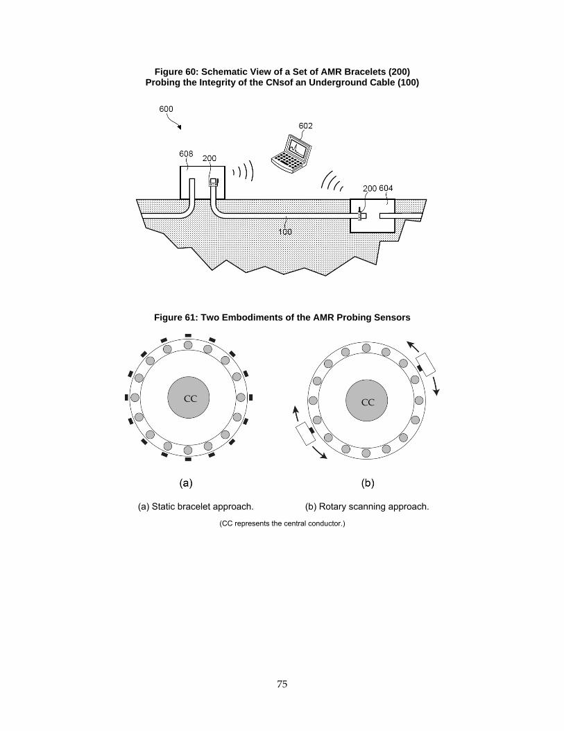
75

Figure 60: Schematic View of a Set of AMR Bracelets (200) Probing the Integrity of the CNsof an Underground Cable (100)

Figure 61: Two Embodiments of the AMR Probing Sensors

(a) Static bracelet approach. (b) Rotary scanning approach.

(CC represents the central conductor.)

CC CC

76

Figure 62: Static AMR Bracelet Fixture Design

(a) Closed configuration (b) open configuration

(The fixture detaches from the hot-stick in the closed configuration (a).)

Figure 63: Exploded View of the Static AMR Bracelet Fixture Design

(a) Closed configuration (b) open configuration

77

Figure 64: Block Diagram of the Electronics for the Static AMR Bracelet Approach

Figure 65: Prototype Flexible Circuit Board Containing Twelve 3-axis AMR Sensors


A block diagram of the electronics is for the rotary scanning approach is shown in Figure 67. A single radio is sufficient to transfer data from a single sensor and back to the data‐collecting laptop. In addition to the sensory information, the position of the rotary device and the control signal to the actuator that moves the movable fixture are transmitted.

4.2.4 Modeling Modeling was performed in MATLAB using the Biot‐Savart law to calculate the compound field emanating from the underground cable. The field was calculated in the circumferential direction (around the circumference of the cable), the radial direction (from the center of the

78

cable and radially out), and in the axial direction along the axis of the cable. Figure 68 illustrates the three magnetic axes in relation to the surface of the cable.

Figure 66: Clamp Fixture for the Deployment of the Rotary Scanning Approach

The clamp contains an inside track (i) that allows an internal roller-supported fixture (ii) to move back and forth. The fixture is pulled by cables that are actuated using a central servo-actuator located in the joint of the clamp (iii).

Figure 67: Block Diagram of the Electronics for the Rotary AMR Probing Approach

4.3.3.1 Static AMR Bracelet The modeling of the static bracelet approach indicates that as long as the number of CNs in the distribution cable is known, a static sensor bracelet will produce a signature that can be used to detect broken CNs. Figure 69 shows the signature from an ideal‐case 10 CN static bracelet with one faulty CN. Figure 70 shows the simulated change in the output of the three axes of the

sensor as the bracelet is misaligned with the CNs. The site of the faulty CN is visible in all cases. An FFT analysis can identify the fault signature at an even higher noise level. A similar result

(i)

(ii)

(ii)

(iii)

79

was obtained when researchers analyzed the relative variability in the physical distribution of CN wires around the cable; such variability is common in commercially produced cables.

Figure 68: The Three Axes for the Magnetic Sensors

The field is measured along the circumferential direction (red), the radial direction (blue), and the axial direction (green).

Figure 69: The Signature of a Single Faulty CN in a 10-CN Cable Using a 10-Sensor Bracelet.

80

4.3.3.2 Rotary AMR Scanning Approach Figure 71 shows the simulation results from the rotary scanning approach in the case of zero broken CNs and 50 A (rms) current passing through the CNs. The peaks corresponding to the individual CNs can be seen. The signatures of the faults are also readily detectable.

Figure 72 shows the simulated fields due to faults in a single CN (left) and four consecutive CNs (right) with a 50 A (rms) current in the CNs. The signatures due to faults (indicated by red arrows) are clearly visible.

Figure 70: Changes in Magnetic Fields with Increasing Relative Misalignment between the Bracelet and the Location of the CNs

(a) Axial direction (b) Circumferential direction

81

Figure 71: Simulation of the Magnetic Fields Emanating from the Cable with50 A (rms) Current in the CNs

(Blue: radial. Red: circumferential. Green: axial.)

Figure 72: Simulated Field Values for a Cable with Broken CNs

(a) Single broken CN. (b) Four broken CNs.


82

Figure 73 shows a failure of two consecutive CNs, simulated using the rms field values. Clearly two peaks can now be seen in the radial field.

Figure 73: Simulated Field Values for a Cable with Two Consecutive Broken CNs


Note that the AMR sensor assembly is recording the rms values of the magnetic fields, and hence the phase information of the current is lost.

4.3.4 Experimental Results 4.3.4.1 Static AMR Bracelet Figure 74 and Figure 75 show the results from testing the static bracelet prototype on a short cable section (3 ft.) with 22 A passing through the CC, and 5 A passing through the CNs. The initial prototype resulted in several failed sensors; consequently only the data from seven sensors are displayed. The figure shows that failure signatures are visible in both the circumferential and axial components of the magnetic field. Because the CC and CN currents are opposing each other, the resulting superposition of magnetic fields causes a signal increase when the current in the faulty CN is zero. The variability due to both misalignment of the sensor and distance between the sensors and the cable is apparent.

83

Figure 74: The Circumferential and Axial Sensor Readings of the Static AMR Bracelet

Figure 75: Radial Sensor Readings of the Static AMR Bracelet

4.3.5 Sensor Prototypes 4.3.5.1 Static AMR Bracelet Researchers developed prototypes of the entire system, consisting of a mechanical fixture design that will clamp around the cable and secure the sensors, the electronics that support the sensor data acquisition over a low‐power radio link, and flexible circuit board that contains the sensors. Figures 62 and 63 showed the designs of the mechanical fixture, operated via a hot‐stick device that can grab the live cable. The fixture is designed to detach from the hot‐stick in the closed configuration. For in‐lab testing, the fixture is fabricated using the 3D rapid prototyping machine in the lab.

Although the static sensor bracelet approach is advantageous in that it does not contain any moving parts, implementation of such an approach using the electronics is much more

84

challenging because of the large amount of data that must be transmitted back to the receiver. Also, as is clearly visible in Figure 75, local misalignments between the sensors and the surface of the cable can produce variations that add to the noise and might be convoluted with the signal from the CNs. A microfabricated bracelet that better conforms to the cable can perhaps avoid this problem altogether. For this reason, researchers concentrated further analysis on the rotary scanning approach.

4.3.5.2 Rotary Scanning Approach The rotary scanning approach was tested on a test‐bed developed in collaboration with the local utilities. Figure 76 shows the test‐bed setup. Researchers performed tests on 100‐ft sections of underground distribution cables. Researchers used a current transformer to generate up to 50 A (rms) of current which was returned via the CNs. Researchers recorded data for 100 percent, 50 percent and 10 percent return current, modeling various load‐imbalance configurations.

Figure 76: View of Cable Test-bed Showing the Rotary Sensor Fixture (at Right)


A manually operated, rapid prototyped fixture was created that would contain the sensor with the attached electronics and radio. Figure 77 shows the design of the fixture (left) and the picture of the rapid‐prototyped fixture (right). The fixture was manually rotated around the cable. Separate fixtures were fabricated to fit jacketed and unjacketed cables. On unjacketed cables, the CN location was constrained using electrical tape to ensure reproducible results across all experiments.

85

Figure 77: The Conceptual Design and the Fabricated Rotary Fixture


4.3.5.2 Rotary Scanning Approach – Jacketed Cable Figure 78 shows the signal from the AMR rotary scan of a healthy jacketed cable with approximately 50 A (rms) flowing through the CC and 100 percent of its current returning through the CNs. The locations of the CNs are designated by the black dashed lines, overlaying the data from the three magnetic axes. However, because the data is converted to rms values before it is transmitted between the sensors, the phase information is lost and the appearance of the additional peaks is visible. In fact, the sensor readings are in the opposite phase, because the CN return current is in the opposite direction of the current flowing through the CC, effectively reducing the field emanating from the CC. However, the rms values do not seem to be centered around zero, but at an offset that seems to vary with the angle of the cable. This is apparent across all measurements, and seems to be an artifact of the measurement technique.

Figures 79 and 80 show data from the 50 percent and 10 percent CC current return experiments, respectively. On the left in both figures, researchers show the data from the maximum current that could be sourced by the setup in this configuration. Such high current, in the absence of a strong negating field emanating from the CNs, tends to saturate the circumferential axis of the AMR sensor, resulting in no visual response. The radial and axial fields are not affected by the CC current. In the 50 percent return current experiment (Figure 79), corresponding to 20 A (rms) return in the CNs, a response in the axial field can be seen. Once the CC current is reduced to approximately 20 A (rms), peaks in the circumferential field appear even though the signal is still close to saturation. In the 10 percent return current experiment (Figure 80), corresponding to 2 A (rms) return in the CNs, the signal is too weak, and no visible signature can be observed.

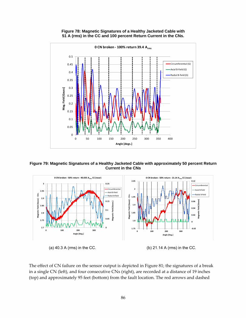
86

Figure 78: Magnetic Signatures of a Healthy Jacketed Cable with 51 A (rms) in the CC and 100 percent Return Current in the CNs.

0

0.05

0.1

0.15

0.2

0.25

0.3

0.35

0.4

0.45

0.5

0 50 100 150 200 250 300 350 400

Mag. Field [G

auss]

Angle [degs.]

0 CN broken ‐ 100% return 39.4 Arms

Circumferential (G)

Axial B‐field (G)

Radial B‐field (G)

Figure 79: Magnetic Signatures of a Healthy Jacketed Cable with approximately 50 percent Return Current in the CNs

0

0.05

0.1

0.15

0.2

0.25

2.7

2.75

2.8

2.85

2.9

2.95

3

0 100 200 300

Magne

tic Field [Gauss.]

Magne

tic Field [Gauss] ‐C

irc.

Angle [Deg.]

0 CN broken ‐ 50% return ‐ 40.035 Arms CC (near)

Circumferential

Axial B‐field

Radial B‐field

‐0.02

0

0.02

0.04

0.06

0.08

0.1

0.12

1.75

1.8

1.85

1.9

1.95

2

2.05

0 100 200 300

Magne

tic Field [Gauss]

Magne

tic Field [Gauss] ‐Circ.

Angle [Deg.]


Circumferential

Axial B‐field

Radial B‐field

(a) 40.3 A (rms) in the CC. (b) 21.14 A (rms) in the CC.

The effect of CN failure on the sensor output is depicted in Figure 81; the signatures of a break in a single CN (left), and four consecutive CNs (right), are recorded at a distance of 19 inches (top) and approximately 95 feet (bottom) from the fault location. The red arrows and dashed

87

lines indicate broken CNs. In this case, the break was induced with 100 percent CC return current.

Figure 80: Magnetic Signatures of a Healthy Jacketed Cable with approximately 10 percent Return Current in the CNs

‐0.05

0

0.05

0.1

0.15

0.2

0.25

2.8

2.82

2.84

2.86

2.88

2.9

2.92

2.94

2.96

2.98

3

0 100 200 300Magne

tic Field [G

auss]

Magne

tic Field [G

auss] ‐C

irc.

Angle [Deg.]


Circumferential

Axial B‐field

Radial B‐field

0

0.02

0.04

0.06

0.08

0.1

0.12

2.1

2.15

2.2

2.25

2.3

2.35

2.4

0 100 200 300

Magne

tic Field [Gauss]

Magne


Angle [Deg.]


Circumferential

Axial B‐field

Radial B‐field

(a) 39.07 A (rms) in the CC. (b) 19.07 A (rms) in the CC.

88

Figure 81: Magnetic Signatures of a Jacketed Cable with approximately 50 A (rms) in the CC and100 percent Return Current in the CNs

0

0.2

0.4

0.6

0.8

1

1.2

1.4

1.6

0 100 200 300

Magne

tic Field [Gauss]

Angle [Deg.]


Circumferential

Axial B‐field

Radial B‐field

0

0.5

1

1.5

2

2.5

3

0 100 200 300

Magne

tic Field [G

auss]

Angle [Deg.]


Circumferential

Axial B‐field

Radial B‐field

0

0.2

0.4

0.6

0.8

1

1.2

0 100 200 300

Magne

tic Field [G

auss]

Angle [Deg.]

1 CN broken ‐ 100% return ‐ 51.4 Arms CC (far)

Circumferential

Axial B‐field

Radial B‐field

0

0.5

1

1.5

2

2.5

3

0 100 200 300

Magne

tic Field [Gauss]

Angle [Deg.]


Circumferential

Axial B‐field

Radial B‐field

Two left graphs: 1 broken CN. Two right graphs: 4 broken CNs. Two top graphs: fault detected at a distance of 19 inches. Two bottom graphs: fault detected at a distance of approx. 95 feet.

Figure 82 is similar to Figure 81, but with CC current of approx. 20 A (rms) and 50 percent return current in the CNs. The fault signatures are still clearly visible.

89


0

0.05

0.1

0.15

0.2

0.25

0.3

1.8

1.85

1.9

1.95

2

2.05

2.1

0 100 200 300

Magne

tic Field [Gauss]

Magne


Angle [Deg.]


Circumferential

Axial B‐field

Radial B‐field

0

0.2

0.4

0.6

0.8

1

1.2

1.4

1.6

1.8

0 100 200 300

Magne

tic Field [Deg.] ‐Circ.

Angle [Deg.]


Circumferential

Axial B‐field

Radial B‐field

0

0.05

0.1

0.15

0.2

0.25

0.3

0.35

1.75

1.8

1.85

1.9

1.95

2

2.05

2.1

2.15

0 100 200 300

Magne

tic Field [G

auss]

Magne

tic Field [G

auss] ‐C

irc.

Angle [Deg.]


Circumferential

Axial B‐field

Radial B‐field

0

0.2

0.4

0.6

0.8

1

1.2

1.4

1.6

1.8

0 100 200 300

Magne

tic Field [Gauss]

Angle [Deg.]


Circumferential

Axial B‐field

Radial B‐field


90

Figure 83 shows the data for the 10 percent CN return case. At 20 A (rms) CC current, researchers see no data indicative of a fault. The signal is reduced below the noise level of the system.

Overall, the data seem to confirm the viability of researchers’ technique to detect faults in jacketed cables. The lower limit of detection for CN current seems to be around 0.5 A (rms) per CN, based on the data. Researchers believe this limit can be further improved with a microfabricated sensor design that is in closer proximity the CNs, and a sensor design that uses magnetic material to enhance the flux emanating from the CNs.


0

0.02

0.04

0.06

0.08

0.1

0.12

2.2

2.25

2.3

2.35

2.4

2.45

0 100 200 300

Magne

tic Field [Gauss]

Magne


Angle [Deg.]


Circumferential

Axial B‐field

Radial B‐field

0

0.02

0.04

0.06

0.08

0.1

0.12

0.14

0.16

0.18

0.2

2.2

2.22

2.24

2.26

2.28

2.3

2.32

2.34

2.36

2.38

0 100 200 300

Magne

tic Field [Gauss]

Magne

tic Field [Gauss] ‐C

irc.

Angle [Deg.]


Circumferential

Axial B‐field

Radial B‐field

‐0.05

0

0.05

0.1

0.15

0.2

0.25

2.1

2.15

2.2

2.25

2.3

2.35

2.4

2.45

2.5

0 100 200 300

Magne

tic Field [Gauss]

Magne


Angle [Deg.]


Circumferential

Axial B‐field

Radial B‐field

0

0.05

0.1

0.15

0.2

0.25

0.3

2.05

2.1

2.15

2.2

2.25

2.3

2.35

2.4

2.45

0 100 200 300

Magne

tic Field [Gauss]

Magne


Angle [Deg.]


Circumferential

Axial B‐field

Radial B‐field


4.3.5.3 Rotary Scanning Approach – Unjacketed Cable Most problematic underground cables are unjacketed, so this diagnostic technique was also tested on unjacketed cables. Figures 84–86 show the baseline plots from the sensor deployed on

91

undamaged unjacketed cable for 100 percent, 50 percent, and 10 percent return currents, respectively. Because the circumferential sensor saturates at approximately 3 Gauss, or about 30 A (rms) CC current when 50 percent or less current is returning through the CNs, Figures 85 and 86 contain results from CC current at 20 A (rms) or less. The locations of the CNs are designated by black dashed lines overlaying the data from the three magnetic axes.

Clearly, irregularities in CN location, due to their movement around the semicon, induce variability to the reading of the AMR sensors. However, a fault signature can still be observed. Figure 87 shows the signatures of breaks in a single CN (left), and four consecutive CNs (right), recorded at a distance of 19 inches (top) and approximately 95 feet (bottom) from the fault location. The red lines and arrows indicate broken CNs. In this case, the break was induced with 100 percent CC return current.

Figure 84: Magnetic Signatures of a Healthy Unjacketed Cable with 49.5 A (rms) in the CC and 100 percent Return Current in the CNs

0

0.2

0.4

0.6

0.8

1

1.2

1.4

1.6

0 100 200 300

Magne

tic field [G

auss]

Angle [Deg.]

Unjacketed 0 CN broken ‐ 49.5 A 100% return (near)

CircumferentialAxial B‐fieldRadial B‐field

92


0

0.05

0.1

0.15

0.2

0.25

0.3

0.35

0.4

0.45

1.65

1.7

1.75

1.8

1.85

1.9

1.95

2

0 100 200 300

Magne

tic field [G

auss]

Magne

tic field [G

auss] ‐C

irc.

Angle [Deg.]

Unjacketed 0 CN broken ‐ 20 A 50% return (near)

Circumferential

Axial B‐field

Radial B‐field


0

0.05

0.1

0.15

0.2

0.25

0.3

0.35

0.4

0.45

2.2

2.25

2.3

2.35

2.4

2.45

2.5

0 100 200 300

Magne

tic field [G

auss]

Magen

tic field [Gauss] ‐C

irc.

Angle [Deg.]


Circumferential

Axial B‐field

Radial B‐field

The variability in CN distribution makes it difficult to detect the fault of a single CN, though at 19 inches from the fault researchers were able to detect a clear signature of the fault of 4 CNs. However, no visible signature is apparent at the far (approximately 95 feet) location from the break point compared with the results from the baseline (healthy cable) at that location (Figure

93

88). This indicates that since the CNs are allowed to touch, the current is transferred from healthy to unhealthy CNs at their contact point. However this is likely an artifact of the experimental setup, because in the test‐bed the cable is coiled, allowing the CNs to touch.

Touching of the CNs in a coiled cable negates the validity of the results for the far location. Figures 89 and 90 show the signatures of breaks in the CNs for 50 percent and 10 percent return current, respectively, taken at the near location only for one broken CN (left in each Figure) and four consecutively broken CNs (right).

Although in the 50 percent CN return case (Figure 89) researchers can see a signature develop as the failure site is expanded to four consecutive CNs, the variability of the CN distribution in unjacketed cables makes it difficult to discern failed concentric neutrals. In the 10 percent return case, the signal from the CNs is weak, although a weak signature may still be observed.

4.3.6 Conclusions Experimental results suggest that the magnetic (AMR) CN probing method may be viable for on‐line detection of CN degradation. In the laboratory setup, researchers were able to detect defects in CNs in jacketed cables (with ordered CN distribution) where the distributed current in all the CNs was 10 A (rms) or more. This corresponded to 50 percent return current in the setup. In the test‐bed, researchers are able to detect the degradation up to the full length of the cables (approximately 95 feet) from the failure site on jacketed cables.

On unjacketed cables, if the CNs are touching each other, the ability to detect the CN failure far from the failure site is reduced. However, researchers believe this was an artifact of the setup, as due to space limitations, a significant portion of the cable was coiled. As the CNs corrode an insulating corrosion layer should form that would reduce the CN contact, and thereby reduce the ability for the current to pass even if the CNs are touching. Furthermore, because the cable is stretched in the duct, fewer CNs are actually touching. The varying distribution of CNs on unjacketed cables also makes it challenging to detect the signature of a failure site, although such signature was clearly observable in the 100 percent return case.

94

Figure 87: Magnetic Signatures of an Unjacketed Cable with approximately 50 A (rms) in the CC and 100 percent Return Current in the CNs

0

0.5

1

1.5

2

2.5

3

0 100 200 300

Magne

tic field [G

auss]

Angle [Deg.]


Circumferential

Axial B‐field

Radial B‐field

0

0.5

1

1.5

2

2.5

3

0 100 200 300

Magne

tic field [Gauss]

Angle [Deg.]



0

0.5

1

1.5

2

2.5

0 100 200 300

Magne

tic fie

ld [Gauss]

Angle [Deg.]

Unjacketed 1 CN broken ‐ 50 A 100% return (far)


0

0.5

1

1.5

2

2.5

3

0 100 200 300

Magne

tic field [G

auss]

Angle [Deg.]

Unjacketed 4 CN broken ‐ 50 A 100% return (far)

Circumferential

Axial B‐field

Radial B‐field


Lastly, the strong influence of the CC current saturating the circumferential axis of the magnetic sensors is also a problem.

Researchers believe the initial results show that the magnetic CN probing method has merit for probing CNs of underground power distribution cables. However, it seems that fabrication of sensors that are in closer contact with the cable and contain flux‐concentrators that direct the magnetic field from the CNs towards the sensor, while dispersing the field from the CC, will greatly improve the sensitivity, reduce the effect on the sensors by the magnetic field from the CC, and ultimately allow this method to be applicable to diagnostics of both jacketed and unjacketed cables. Researchers also believe that the benefits of the static bracelet approach should be explored further. Specifically, electronics should be developed that would allow proper multiplexing and perhaps pre‐processing of the 30 channels (3 axis per CN, assuming 10 CNs) that need to be transmitted to the recording laptop.

95

Figure 88: Magnetic Signature of a Healthy Unjacketed Cable with 49.8 A (rms) in the CC and 100 percent Return Current in the CNs, Measured at the Far Location (approximately 95 feet)

0

0.5

1

1.5

2

2.5

3

0 100 200 300

Magne

tic field [Gauss]

Angle [Deg.]

Unjacketed 0 CN broken ‐ 49.8 A 100% return (far)


Figure 89: Magnetic Signatures of a Jacketed Cable with approximately 20 A (rms) in the CC and 50 percent Return Current, with Broken CNs Detected 19 in. from the Fault Site

0

0.1

0.2

0.3

0.4

0.5

0.6

0.7

0.8

2.8

2.82

2.84

2.86

2.88

2.9

2.92

2.94

2.96

2.98

3

0 100 200 300

Magne

tic field [G

auss]

Magne

tic field [G

auss] ‐C

irc.

Angle [Deg.]


Circumferential

Axial B‐field

Radial B‐field

0

0.2

0.4

0.6

0.8

1

1.2

1.4

1.6

1.8

2

2.82

2.84

2.86

2.88

2.9

2.92

2.94

2.96

2.98

3

0 100 200 300

Magne

tic field [G

auss]

Magne

tic field [G

auss] ‐C

irc.

Angle [Deg.]



96

Figure 90: Magnetic Signatures of a Jacketed Cable with approximately 20 A (rms) in the CC and 10 percent Return Current, with Broken CNs Detected 19 in. from the Fault Site

‐0.05

0

0.05

0.1

0.15

0.2

0.25

0.3

2.15

2.2

2.25

2.3

2.35

2.4

2.45

2.5

0 100 200 300

Magne

tic field [Gauss]

Magne

tic fie

ld [Gauss] ‐Circ.

Angle [Deg.]


Circumferential

Axial B‐field

Radial B‐field

‐0.05

0

0.05

0.1

0.15

0.2

0.25

0.3

2.1

2.15

2.2

2.25

2.3

2.35

2.4

2.45

2.5

0 100 200 300

Magne

tic field [G

auss]

Magne

tic field [G

auss] ‐C

irc.

Angle [Deg.]

Unjacketed 4 CN broken ‐ 20.55 A 10% return (near)

Circumferential

Axial B‐field

Radial B‐field

97

CHAPTER 5: Concluding Discussion 5.1 Summary The aging of installed underground distribution cables is a looming issue facing electric utilities in California and throughout the U.S. A variety of technologies and tests are currently available to evaluate underground cables, but there is often little correlation between the diagnostic results and the actual deterioration. This project evaluated the problem of underground cable failure and researched innovating online techniques for diagnosing failing underground cables.

Researchers investigated several failure mechanisms for the insulation of underground power distribution cables. Researchers revised Zeller’s models for the development of water trees within PE, and found that cyclic dielectrophoretic stresses around defects such as voids or inclusions, is a possible mechanism for the development of water trees. Researchers have also found that charges can be injected into PE, which may enhance the breakdown of PE and the formation of water trees. Overall, researchers can conclude that the mechanism of water treeing is complex, and largely influenced by several mechanical and electrochemical factors. Further work should be dedicated to the investigation these phenomena.

On the diagnostic method side, researchers investigated four potential methods for online diagnosis of underground power distribution cables. Two methods, interdigitated dielectrometry and surface‐guided RF probing (Goubau) were abandoned, deemed to insufficiently practical at the time, although researchers believe they merit to be revisited in the future. The two remaining techniques, RF‐test point injection and the magnetic CN (AMR) probing, have great future merit as online diagnostic techniques.

Researchers have shown that researchers can couple and transmit an RF signal through an energized power distribution cable. The lack of a positive result is believed to be attributable to lack of a proper water‐treed cable for testing. The investigation of this method should be continued once a suitable water‐treed cable has been found.

The magnetic CN (AMR) probing has experimentally been shown to identify failure signatures far (at least 95 feet) from failure location. Further work needs to be performed to enhance the sensitivity of this method to magnetic field stemming from CN currents, while reducing its sensitivity to the CC current. Microfabricated sensors and flux‐concentrators should be able to achieve this goal. Furthermore, the CN magnetic probing method needs to be combined with a method to detect the location of the CNs, to determine whether the lack of magnetic field is attributed to a broken, or simply the lack of CN at that location. This is specifically important in unjacketed cables, where the CN location can be highly variable.

Ultimately, researchers envision both the RF test‐point injection probing and the magnetic CN (AMR) probing techniques to be used together as a comprehensive diagnostic method for online testing of the health of underground power distribution cables. Figure 91 shows a conceptual overview of a possible implementation of such a composite cable diagnostics method. The data

98

is envisioned displayed on a customized FieldFox network analyzer (image courtesy of Agilent Technologies Inc.).

Figure 91: An Envisioned Comprehensive Underground Cable Diagnostic Method, with RF Test-Point Injection Probing and Magnetic CN (AMR) Probing

Photo Credits: Agilent Technologies Inc.

5.2 Recommendations Both the RF test‐point injection probing and the magnetic CN (AMR) probing methods show merit as online diagnostic techniques for underground power distribution cables. Researchers recommend further work on both techniques to bring the two methods closer to systems that can ultimately be used in the field.

The RF test‐point injection probing method needs to be evaluated on cables known to contain water trees. Both jacketed and unjacketed water‐treed cables need to be evaluated, and also compared to cables with no water trees, to establish a baseline for the failure signature of this technique. This should be done in collaboration with utilities that have an ongoing asset management and replacement program.

The Magnetic CN (AMR) probing method has been shown to detect defects in CNs of underground cables. In the future, microfabricated sensors and flux concentrators that magnify the magnetic flux from the CNs while diverting the magnetic flux emanating from the CC should be developed. Together with a sensor that detects the location of the individual sensors, this technique should be able to detect CN failure in a large range of CN return current and

99

imbalance current conditions. Furthermore, microfabrication of these sensors, combined with AC energy harvesting techniques, such as described in Paprotny et al. (2010), will allow self‐powered wireless operation of these sensors that can continuously monitor the performance of underground power distribution assets.

5.3 Publications Publications related to or arising from this work (Chapter 7, References) include:

Gonzalez, Paprotny, White and Wright (2011)

Paprotny, Seidel, Nora, Morris, White and Wright (2012)

Paprotny, White and Krishnan (2010)

Paprotny, White and Wright (2010)

Seidel, Paprotny, White and Krishnan (2010)

Zhou and Boggs (2011)

100

GLOSSARY

AC alternating current

AIEE American Institute of Electrical Engineers (precursor to IEEE)

AMR amorphous magneto‐resistive

ASTM American Society for Testing and Materials

CAD computer‐aided design

CC central conductor

CN concentric neutral

DC direct current

eV electron Volt (unit of energy)

FE finite element

GW Goubau wave

HDPE high‐density polyethylene

Hz Hertz (measure of frequency)

ID interdigitated dielectrometry

IEEE Institute of Electrical and Electronics Engineers

J Joule (unit of energy)

kV kiloVolt

L liter

LDPE low‐density polyethylene

Pa Pascal (unit of pressure or stress)

PG&E Pacific Gas & Electric Co.

PIER Public Interest Energy Research

PE polyethylene

PVC polyvinyl chloride

RF radio frequency

RD&D research, development, and demonstration

rms root mean square

S Siemens (unit of conductivity)

SDG&E San Diego gas & Electric Co.

TD time domain

101

TR‐XLPE tree‐retardant cross‐linked polyethylene

U/G underground

XLPE cross‐linked polyethylene

102

REFERENCES

Anta, J. A., G. Marcelli, M. Meunier and N. Quirke, “Models of Electron Trapping and Transport in Polyethylene: Current‐Voltage Characteristics,” Journal of Applied Physics, Vol. 92, pp. 1002–1008, 2002.

ASTM International, “Standard Test Method for Tensile Properties of Plastics,” D638–08, 2008.

Beaumont, J. H. and P. W. M. Jacobs, “Polarization in Potassium Chloride Crystals,” Journal of Physics and Chemistry of Solids, Vol. 28, pp. 657–667, 1967.

Boggs, S., “On‐axis Field Approximations for a (Semi‐)Spheroid in a Uniform Field,” IEEE Transactions on Dielectrics and Electric Insulation, Vol. 10, pp. 305–306, 2003.

Boggs, S. A., J. Kuang and J. Jow, “Numerical Computational of the Chemical Potential for Water Tree Initiation and Growth,” unpublished work, 1995–1996.

Cole, K. S. and R. H. Cole, “Dispersion and Absorption in Dielectrics II: Direct Current Characteristics,” Journal of Chemical Physics, Vol. 10, pp. 98–105, 1942.

Delleur, J. W., ed., The Handbook of Groundwater Engineering, 2nd Edition, CRC Press, Chapter 17, 2007.

Dodson, R. W., “The Exchange Relation Between Ferrous and Ferric Ions in Perchloric Acid,” Journal of the American Chemical Society, Vol. 70, pp. 3315–3316, 1950.

Dubickas, V. and Edin, H., “Dielectric Model of Water Trees in an XLPE Cable,” Proceedings of the International Symposium on Electrical Insulation Materials, pp. 448–451, 2008.

East Bay Municipal Utility District (EBMUD), “2009 Annual Water Quality Report.” Available at: http://www.ebmud.com/sites/default/files/pdfs/2009_annual_water_quality_report_1.pdf

Fabiani, D., G. C. Montanari, A. Cavallini and G. Mazzanti, “Relation Between Space Charge Accumulation and Partial Discharge Activity in Enameled Wires Under PWM‐like Voltage Waveforms,” IEEE Transactions on Dielectrics and Electrical Insulation, vol. 11, no. 3, pp. 393–405, June 2004.

Das Gupta, D. K. and R. S. Brockley, “A Study of ‘Absorption Currents’ in Low Density Polyethylene,” Journal of Physics D: Applied Physics, Vol. 11, pp. 955–962, 1978.

Given, M. J., R. A. Fouracre, S. J. MacGregor, M. Judd and H. M. Banford, “Diagnostic Dielectric Spectroscopy Methods Applied to Water‐treed Cable,” IEEE Transactions on Dielectrics and Electric Insulation, vol. 8, no. 6, pp. 917–920, Dec. 2001.

Gonzalez, G., I. Paprotny, R. M. White and P. K. Wright, “Novel Online RF Technique for Detection of Water Trees in Underground Powered Distribution Cables,” Proceedings of the 2011 IEEE International Symposium on Electrical Insulation (ISEI 2011), pp. 345–348, June 5‐8, 2011.

103

Goubau, G., “Surface Waves and Their Applications to Transmission Lines,” Journal of Applied Physics, Vol. 21, 1950.

Hoffmann, R., C. Janiak and C. Kollmar, “A Chemical Approach to the Orbitals of Organic Polymers,” Macromolecules, Vol. 24, pp. 3725–3746, 1991.

Huzayyin, A., S. Boggs and R. Ramprasad, “Effect of Carbonyl Impurities on Polyethylene Band Structure Using Density Functional Theory,” IEEE Conference on Electrical Insulation and Dielectric Phenomena (CEIDP), pp. 353‐356, 2008.

Hvidsten S., E. Ildstad, J. Sletbak and H. Faremo, “Understanding Water Treeing Mechanisms in the Development of Diagnostic Test Methods,” IEEE Transactions on Dielectrics and Electric Insulation, 5(5), pp. 754‐760, Oct. 1998.

Institute of Electrical and Electronics Engineers, IEEE Guide for Detection, Mitigation, and Control of Concentric Neutral Corrosion in Medium‐Voltage Underground Cables, IEEE Standard 1617‐2007, Feb. 2007.

Kahn, D. and J.N. Maycock, “Difference Equation Model for Ionic Conductivity: I. Step Voltage Response,” Journal of Chemical Physics, Vol. 46, pp. 4434‐4440, 1967.

Kallmann, H. and M. Pope, “Positive Hole Injection into Organic Crystals,” Journal of Chemical Physics, Vol. 32, pp. 300‐301, 1960.

Kallmann, H. and M. Pope, “Surface‐controlled Bulk Conductivity in Organic Crystals,” Nature, Vol. 186, No. 4715, p. 753, 1960.

Kitchin, D. W. and O. S. Pratt, “Treeing in Polyethylene as a Prelude to Breakdown,”AIEE Transactions on Power Apparatus and Systems, vol. 77, p. 180, 1958.

Koo, J. Y., J. D. Cross, M. El‐Kahel, C. T. Meyer and J. C. Filippini, “Electrical Behavior and Structure of Water Trees in Relation to their Propagation,” Annual Report Conference on Electrical Insulation and Dielectric Phenomena, IEEE Publication 83CH19831902‐6, pp. 301‐306, 1983.

Landau, L. D., L. P. Pitaevskii and E. M. Lifshitz, Electrodynamics of Continuous Media, 2nd edition, Vol. 8 (Course of Theoretical Physics), Oxford: Butterworth‐Heinemann, chapter 2, pp. 44‐51, 1984.

Lengyel, G., “Schottky Emission and Conduction in Some Organic Insulating Materials,” Journal of Applied Physics, Vol. 37, pp. 807‐810, 1966.

Less, K. J. and E. G. Wilson, “Intrinsic Photoconduction and Photoemission in Polyethylene,” Journal of Physics C: Solid State Physics, Vol. 6, pp. 3110‐3121, 1973.

Lewis, T. J., “Polyethylene under Electrical Stress,” IEEE Transactions on Dielectrics and Electric Insulation, Vol. 9, pp. 717‐729, 2002.

Lilly, A. C., D. A. Lowitz, and J. C. Shug, “Space Charge Conduction in Insulators,” Journal of Applied Physics, Vol. 39, pp. 4360‐4364, 1968.

104

Lilly, A. C. and J. R. McDowell, “High‐Field Conduction in Films of Mylar and Teflon,” Journal of Applied Physics, Vol. 39, pp. 141–147, 1968.

Lohmann, F. and W. Mehl, “Organic Crystal‐Electrolyte Interface,” Progress in Surface Science, Elsevier Press, Vol. 6, No. 3, pp. 185–212, 1975.

Macdonald, J. R., “Electrical Response of Materials Containing Space Charge with Discharge at the Electrodes,” Journal of Chemical Physics, Vol. 54, pp. 2026–2050, 1971.

Mayashita, T. and T. Inoue, “The Study of Tree‐deterioration Mechanism of Water‐immersed Polyethylene Coated Wire,” Japanese Institute of Electrical Engineering, vol. 48‐10, p. 161, 1967.

McAllister, I. W., G. C. Crichton and A. Pedersen, “Charge Accumulation in DC Cables: A Macroscopic Approach,” Conference Record of the 1994 IEEE International Symposium on Electrical Insulation (ISEI), Pittsburgh, PA, pp. 212–216, 1994.

McCall, D., D. Douglass and L. Blyler Jr., “Solubility and Diffusion of Water in Low‐density Polyethylene,” Macromolecules, Vol. 17, pp. 1644–1649, 1984.

Mehl, W. and J. M. Hale, Advances in Electrochemistry, Vol. 6, Wiley‐Interscience: New York, p. 399, 1967.

Meunier, M. and N. Quirke, “Molecular Modeling of Electron Trapping in Polymer Insulators,” Journal of Chemical Physics, Vol. 113, pp. 369–376, 2000.

Meunier, M. and N. Quirke, “Molecular Modeling of Electron Traps in Polymer Insulators: Chemical Defects and Impurities,” Journal of Chemical Physics, Vol. 115, pp. 2876–2881, 2001.

Meyer, C. T. and A. Chamel, “Water and Ion Absorption by Polyethylene in Relation to Water Treeing,” IEEE Transactions on Dielectrics and Electric Insulation, Vol. 15, pp.389–393, 1980.

Mizutani, T. and M. Ieda, “Carrier Transport in High‐Density Polyethylene,” Journal of Physics D: Applied Physics, Vol. 12, pp. 291–296, 1979.

Mizutani, T., T. Tsukahara and M. Ieda, “The Effects of Oxidation on the Electrical Conduction of Polyethylene,” Journal of Physics D: Applied Physics, Vol. 13, pp. 1673–1679, 1980.

Mizutani, T., K. Mitani and M. Ieda, “Influence of Antistatic Agent on Electrical Conduction of Polyethylene,” Japanese Journal of Applied Physics, Vol. 22, pp. 677–680, 1983.

Moreau, E., C. Mayoux, C. Laurent and A. Boudet, “The Structural Characteristics of Water Trees in Power Cables and Laboratory Specimens,” IEEE Transactions on Dielectrics and Electric Insulation, Vol. 28, pp. 54–64, 1993.

Morrison, S. R., Electrochemistry at Semiconductor and Oxidized Metal Electrodes, Plenum Press, New York, USA, p. 32, 1980.

105

Neagu, R. M., E. Neagu, A. Kyritsis and P. Pissis, “Dielectric Studies of Dipolar Relaxation Processes in Nylon 11,” Journal of Physics D: Applied Physics, Vol. 33, pp. 1921–1931, 2000.

Newman, J. S. and K. E. Thomas‐Alyea, Electrochemical Systems, 3rd edition, John Wiley & Sons, Inc., Chapter 11, pp. 283–285, 2004.

Nikolajevic, S. V. and R. Drca, “Effect of Water on Aging of XLPE Cable Insulation,” Electric Power Systems Research, vol. 60, pp. 9–15, 2001.

O’Dwyer, J. J., “Current‐Voltage Characteristics of Dielectric Films,” Journal of Applied Physics, Vol. 37, pp. 599–601, 1966.

Papazyan, R. and R. Eriksson, “High Frequency Characterization of Water‐treed XLPE Cables,” Proceedings of the 7th International Conference on Properties and Applications of Dielectric Materials, pp. 187–190, June 2003.

Paprotny, I., M. Seidel, T. C. Nora, C. Morris, R. M. White and P.K. Wright, “Deployment Methods for Magnetic Integrity Testing of Concentric Neutral Wires in Energized Underground Power Distribution Cables,” to be published in the Conference Record of the 2012 IEEE International Symposium on Electrical Insulation (ISEI 2012), June 10–13, 2012.

Paprotny, I., R. M. White and K. Krishnan, “RF Transmission‐line Methods for In‐service Probing of Concentric Neutral Wires in Underground Power Distribution Cables,” Conference Record of the 2010 IEEE International Symposium on Electrical Insulation (ISEI 2010), pp. 1–5, June 6–9, 2010.

Paprotny, I., R. M. White and P. K. Wright, “Modeling, Design and Fabrication of (10x10x4 mm3) MEMS AC Energy Harvester for Smart Grid Applications,” Proceedings of POWERMEMS 2010, November 30 – December 3, 2010.

Ponniran, A. and M. S. Kamarudin, “Study on the Performance of Underground XLPE Cables in Service Based on Tan Delta and Capacitance Measurements,” IEEE 2nd Annual Power and Energy Conference, pp. 39–43, Dec. 2008.

Pruitt, L., R. Hermann and S. Suresh, “Fatigue Crack Growth in Polymers Subjected to Fully Compressive Cyclic Loads,” Journal of Materials Science, vol. 27, pp. 1608–1616, 1992.

Reid, C. N., K. Williams and R. Hermann, “Fatigue in Compression,” Fatigue of Engineering Materials and Structures, vol. 1, pp. 267–270, 1979.

Rittel, D. and Y. Rabin, “An Investigation of the Heat Generated During Cyclic Loading of Two Glassy Polymers. Part II: Thermal Analysis,” Mechanics of Materials, vol. 32, pp. 149–159, 2000.

Romanets, R. and K. Yoshino, “Transient Currents in Organic Dielectric Liquids, Polymers, and Liquid Crystals,” Ukrainian Journal of Physics, Vol. 49, pp. A55–A60, 2004.

Rose, A., “Space‐charge‐limited Currents in Solids,” Physics Review, Vol. 97, pp. 1538–1544, 1955.

106

Ross, R., “Inception and Propagation Mechanisms of Water Treeing,” IEEE Transactions on Dielectrics and Electric Insulation, Vol. 5, pp. 660–680, 1998.

Samat, N., R. Burford, A. Whittle and M. Hoffman, “The Effects of Water and Frequency on Fatigue Crack Growth Rate in Modified and Unmodified Polyvinyl Chloride,” Polymer Engineering & Science, vol. 50, no. 2, pp. 352‐264, Sept. 2009.

Sauer, J. A., E. Foden and D. R. Morrow, “Influence of Molecular Weight on Fatigue Behavior of Polyethylene and Polystyrene,” Polymer Engineering and Science, vol. 17, no. 4, pp. 246–250, Apr. 1977.

Sauer, J. A. and G. C. Richardson, “Fatigue of Polymers,” International Journal of Fracture, vol. 16, no. 16, pp. 499–532, Dec. 1980.

Seidel, M., I. Paprotny, R. M. White and K. Krishnan, “AMR Current Sensors for Evaluating the Integrity of Concentric Neutrals in In‐Service Underground Power Distribution Cables,” Conference Record of the IEEE International Symposium on Electrical Insulation (ISEI 2010), June 6–9 2010.

Serra, S., E. Tosattil, S. Iarlori, S. Scandolo, G. Santoro and M. Albertini, “Interchain States and the Negative Electron Affinity of Polyethylene,” IEEE Conference on Electrical Insulation and Dielectric Phenomena (CEIDP), Vol. 1, pp. 19–22, 1998.

Smith, R. W. and A. S. Rose, “Space‐charge‐limited Currents in Single Crystals of Cadmium Sulfide,” Physics Review, Vol. 97, pp. 1531–1536, 1955.

Suzuoki, Y., H. Muto, G. Cai, T. Mizutani and M. Ieda, “Effects of Polar Groups on Electrical Conduction in Polyethylene,” Japanese Journal of Applied Physics, Vol. 23, pp. 91–92, 1984.

Suzuoki, Y., H. Muto, T. Mizutani and M. Ieda, “Effects of Space Charge on Electrical Conduction in High‐Density Polyethylene,” Journal of Physics D: Applied Physics, Vol. 18, pp. 2293–2302, 1985.

Taylor, D. M. and T. J. Lewis, “Electrical Conduction in Polyethylene Terephthalate and Polyethylene,” Journal of Physics D: Applied Physics, Vol. 4, pp. 1346–1357, 1971.

Teyssedre, G., C. Laurent, A. Aslanides, N. Quirke, L.A. Dissado, G.C. Montanari, A. Campus and L. Martinotto, “Deep Trapping in Crosslinked Polyethylene Investigated by Molecular Modeling and Luminescence Techniques,” IEEE Transactions on Dielectrics and Electric Insulation, Vol. 8, pp. 744–754, 2001.

Thomas, A. J. and T. K. Saha, “A New Dielectric Response Model for Water Tree Degraded XLPE Insulation – Part A: Model Development with Small Sample Verification,” IEEE Transactions on Dielectrics and Electric Insulation, 15(4), pp. 1131–1143, Aug. 2008.

Thomas, A. J. and T. K. Saha, “A New Dielectric Response Model for Water Tree Degraded XLPE Insulation – Part B: Dielectric Response Verification,” IEEE Transactions on Dielectrics and Electric Insulation, 15(4), pp. 1144–1152, Aug. 2008.

107

Tiebensky, G. N. and H. J. Wintle, “Surface Polarization Capacitance of KBr Single Crystals,” Journal of Physics and Chemistry of Solids, Vol. 33, pp. 191–203, 1972.

Toyoda T., S. Mukai, Y. Ohki, Y. Li and T. Maeno, “Estimation of Conductivity and Permittivity of Water Trees in PE from Space‐charge Distribution Measurements,” IEEE Transactions on Dielectrics and Electric Insulation, 8(1), Feb. 2001, pp. 111–116.

University of the State of New York (USNY), The State Education Department, “Earth Science Reference Tables,” p. 11, 2001. Available at http://www.eduware.com/ESref.pdf.

Weaver, J. L. and C. L. Beatty, “The Effect of Temperature on Compressive Fatigue of Polstyrene,” Polymer Engineering and Science, vol. 18, no. 14, pp. 1117–1126, Mid‐Nov. 1978.

Werelius, P., P. Tharning, R. Eriksson, B. Holmgren and U. Gafvert, “Dielectric Spectroscopy for Diagnosis of Water Tree Deterioration in XLPE Cables,” IEEE Transactions on Dielectrics and Electric Insulation, 8(1), Feb. 2001, pp. 27–42.

Wintle, H. J., “Absorption Current, Dielectric Constant, and Dielectric Loss by the Tunneling Mechanism,” Journal of Applied Physics, Vol. 44, pp. 2514–2519, 1973.

Wintle, H. J., “Absorption Currents and Steady‐State Currents in Polymer Dielectrics,” Journal of Non‐Crystalline Solids, Vol. 15, pp. 471–486, 1974.

Wintle, H. J., “Charge Motion in Technical Insulators: Facts, Fancies and Simulations,” IEEE Transactions on Dielectrics and Electric Insulation, Vol. 10, pp. 826–841, 2003.

Xu, J. and S. Boggs, “The Chemical Nature of Water Treeing: Theories and Evidence,” IEEE Electrical Insulation Magazine, Vol.10, No. 5, pp. 29–37, 1994.

Yoshimura, N., F. Noto and K. Kikuchi, “Growth of Water Trees in Polyethylene and Silicone Rubber by Water Electrodes,” IEEE Transactions on Dielectrics and Electric Insulation, vol. EI‐12, no. 6, pp. 411–416, Dec. 1977.

Zeller, H., “Thermodynamics of Water Treeing,” IEEE Transactions on Dielectrics and Electric Insulation, vol. E1‐22, no. 6, pp. 677–681, Dec. 1987.

Zeller, H., “Noninsulating Properties of Insulating Materials,” IEEE Conference on Electrical Insulation and Dielectric Phenomena (CEIDP), Knoxville, TN, USA, pp. 19–30, 1991.

Zhou, K. and S. Boggs, “Analytical Computations of the Chemical Potential for Water‐Filled Spheroidal Particle, and Comparison with Finite Element Computations,” manuscript in preparation, 2011.

fault analysis in underground cables - california energy ... · pdf filefault analysis in...

Documents