FATIGUE LIFE ASSESSMENT OF A CRITICAL FIELD WELDED

CONNECTION ON A TEMPORARY RAILWAY

BRIDGE SPAN

by

CURTIS HEINSEN

Presented to the Faculty of the Graduate School of

The University of Texas at Arlington in Partial Fulfillment

Of the Requirements for the Degree of

MASTER OF SCIENCE IN CIVIL ENGINEERING

THE UNIVERSITY OF TEXAS AT ARLINGTON

MAY 2015

ii

Copyright © by CURTIS HEINSEN 2015

All Rights Reserved

iii

Acknowledgments

This thesis is the product of a convergence in my professional and academic

careers. It has been a challenging lesson in the art of academic research and time

management. Through the course of this research I have discovered and studied a

number of concepts and principles that I am confident will serve me well throughout my

career. However, without the support and guidance of a number of certain individuals I

can say with absolute confidence that I could never have made it this far in my life either

professionally or academically and I would like to dedicate this research to those people.

First among those that I must sincerely thank is Dr. Ali Abolmaali. In my time

studying the science of engineering I have found Dr. Abolmaali’s lessons to be the most

challenging and the most thought provoking. It was because of his class in the

fundamentals of the finite element method that I first began to take a real interest in the

use of FEM. He has been more than generous in terms of allowing me all the resources I

needed to conduct meaningful research and incredibly flexible by allowing me to conduct

my research while pursuing my career. His guidance has proved invaluable and I know I

would not be where I am now without his help.

I would also like to express my deepest gratitude to Dr. Mohammad Razavi who

supervised my thesis and provided me with unparalleled support and encouragement. Dr.

Razavi provided valuable assistance and advice from the time I began my research and

his comments and suggestions have been essential to my success.

iv

I would also like to thank Dr. Leininger and Dr. Mattingly who presided over

some of my first classes in engineering and who both were very supportive of my goal to

attain a Master of Science degree.

I would also like to acknowledge the role of my colleagues in the field of railway

engineering who provided me with their insight into my research and who have always

shown a great deal of faith in my abilities. Without their valuable input this research

would have proven to be much more challenging.

Lastly I would like to thank my friends and family including my two sisters and

my friends Ryan and Eric who have always been around to help me in all things. Finally

I want to thank my parents. I cannot say enough about how much I owe them both for all

of my accomplishments and so I can only say thank you and hope that they both know

how much their support has meant, and continues to mean.

Thank you all.

April 4, 2015

v

Abstract

FATIGUE LIFE ASSESSMENT OF CRITICAL FIELD WELDED

CONNECTION ON A TEMPORARY RAILWAY

BRIDGE SPAN

CURTIS HEINSEN

The University of Texas at Arlington

Supervising Professor: Mohammad Razavi

There is a need in the railway industry for a flexible solution to the problem of

service interruptions due to impacts on railway bridges from highway and other vehicle

traffic. One such solution is the placement of a temporary span that can be used on

multiple substructure types and configurations and can be quickly assembled from a kit

of available parts. In order to minimize the erection time and maximize the span

flexibility such a span could utilize welded connections in place of bolted connections

throughout the structure. These connections would be vulnerable to fatigue failure which

has been shown in the AREMA design manual as well as various literature to be the

primary limiting factor on the effective lifespan of most steel railway structures including

the temporary span. This thesis analyzes such a structure using the finite element method

vi

and attempts to determine the controlling fatigue life for any number of reasonable

configurations in which the span is likely to be utilized. Then a determination is made as

to whether the design is valid for use in an emergency situation where a replacement

structure could take months or even years to design, fabricate and construct. Phase 1 of

this study leverages the finite element analysis capability of RISA 3D to determine the

location of the most fatigue vulnerable connection in all of the considered configurations

of the temporary span. Multiple load cases are considered including the controlling

“315K” railcar. From this analysis an acceptable approximation of the real life forces

the connection is subjected to can be obtained as well as a good idea of the applied forces

and cycle frequency experienced by the connection. Phase 2 of this study utilizes the

finite element method (FEM) functionality of ABAQUS to obtain parameters necessary

for the completion of a comprehensive fatigue analysis. Parameters that were obtained

during the analysis include the effective stress range (ΔSre) at the toe of the fillet weld in

the critical connection, the stress intensity factors for a crack at the toe of the weld (KI,

KII, KIII), and the residual stresses induced by an arc welding procedure (σres). Phase 3 of

this study utilizes the principles of linear elastic fracture mechanics to propose a

procedure for the estimation of the fatigue life of the critical connection in terms of

number of cycles to failure both considering and neglecting residual stress effects.

Finally, the significance of this research relative to the usefulness of the temporary span

is discussed and recommendations regarding how to leverage the results of this research

for real world use cases of the temporary span are put forward.

vii

Table of Contents

Acknowledgments.............................................................................................................. iii

Abstract ............................................................................................................................... v

List of Figures ..................................................................................................................... x

List of Tables ................................................................................................................... xiv

Chapter 1 Introduction ........................................................................................................ 1

1.1 Background ............................................................................................................... 1

1.2 Literature Review ...................................................................................................... 2

1.2.1 Temporary Spans and Rapid Bridge Replacement Techniques ......................... 3

1.2.2 Fatigue and Fracture Mechanics ........................................................................ 5

1.2.3 Finite Element Analysis ..................................................................................... 7

1.3 Overview of Alternative Efforts to Implement Rapid Bridge Replacement

Techniques ...................................................................................................................... 9

1.3.1 Span by Span Placement Method Using Existing Material ............................... 9

1.3.2 Prefabricated Modular Temporary Span Method (Acrow Panel Bridge) ........ 12

Chapter 2 Design of Temporary Structure ........................................................................ 18

2.1 Dead Load (E-65) .................................................................................................... 22

2.2 Live Load (E-65) ..................................................................................................... 24

2.3 Combined Factored Loads (E-65) ........................................................................... 25

viii

2.4 Tension Stress Check .............................................................................................. 26

2.5 Compression Stress Check ...................................................................................... 27

2.6 Shear Stress Check .................................................................................................. 29

2.7 Initial Overview of Fatigue for Temporary Span .................................................... 30

2.7.1 Use of Finite Element Analysis to Achieve Meaningful Results .................... 34

Chapter 3 Modelling of Temporary Span in RISA 3D ..................................................... 38

3.1 Forces ...................................................................................................................... 42

3.1.1 Dead Load ........................................................................................................ 43

3.1.2 Live Load ......................................................................................................... 44

3.1.3 Impact Load ..................................................................................................... 50

3.1.4 Centrifugal Forces ............................................................................................ 59

3.1.5 Longitudinal Forces ......................................................................................... 63

Chapter 4 FEM Results from Macro Analysis Using RISA 3D ....................................... 65

4.1 55’ Span – Tangent Substructure – 315K Railcars ................................................. 67

Chapter 5 Modelling of Critical Connection Using Abaqus CAE .................................... 76

5.1 Stresses Due to Applied Loads................................................................................ 76

5.2 Residual Stresses Induced by Weld ........................................................................ 80

5.2.1 Thermal Heat Effects Caused by Welding ....................................................... 82

5.2.2 Residual Stresses .............................................................................................. 84

ix

5.2.3 FEM Procedure ................................................................................................ 85

5.2.4 FEM Results..................................................................................................... 86

Chapter 6 Fatigue Life Assessment Utilizing LEFM ....................................................... 93

6.1 Overview of Linear Elastic Fracture Mechanics ..................................................... 93

6.2 Defects in the Critical Connection .......................................................................... 99

6.3 Stress Intensity Factor at the Critical Connection Due to Applied Loads ............ 100

6.4 Stress Intensity Factor at the Critical Connection Due to Residual Stresses ........ 104

6.5 Fracture Toughness, Coefficient of Crack Growth and Critical Crack Length .... 105

6.6 Results and Number of Cycles to Failure ............................................................. 109

6.6.1 Crack Propagation along the Surface of the Web .......................................... 110

6.6.2 Crack Propagation into Thickness of Material .............................................. 111

6.7 Discussion of Results ............................................................................................ 112

Chapter 7 Summary, Conclusions and Future Work ...................................................... 116

7.1 Summary ............................................................................................................... 116

7.2 Conclusions ........................................................................................................... 119

7.3 Future Work .......................................................................................................... 120

References ....................................................................................................................... 122

Biographical Information ................................................................................................ 129

x

List of Figures

Figure 1 - Damage from Impact.......................................................................................... 2

Figure 2 - Existing, Temporary and Permanent Spans for Alkire Road Bridge Project ..... 5

Figure 3 - Span by Span Placement Method for an Emergency Application ................... 11

Figure 4 - Plan and Elevation of Acrow 700XS Customized for Railway Loads [39] ..... 13

Figure 5 - Acrow Bridge Assembly .................................................................................. 14

Figure 6 - Acrow Bridge Crane Pick ................................................................................ 14

Figure 7 - Incremental Launching Method Using Acrow 700XS [40] ............................. 15

Figure 8 - 2-8-0 Consolidation-type Locomotive - Basis for Cooper's E loading [8] ...... 20

Figure 9 - Diagram of Cooper's E-80 Loading for Modern Railway Bridges [1] ............ 20

Figure 10 - Plan of Temporary Span................................................................................. 21

Figure 11 - Moment in Beams Due to Self-Weight and Superimposed Dead Load......... 23

Figure 12 - Shear in Beams Due to Self-Weight and Super Imposed Dead Load ............ 23

Figure 13 - Moment Induced by Cooper's E-65 Load ...................................................... 24

Figure 14 - Shear Induced by Cooper's E-65 Load ........................................................... 25

Figure 15 - Moment Due to Total Combined Loads + Impact ......................................... 26

Figure 16 - Shear Due to Total Combined Loads + Impact .............................................. 26

Figure 17 - Tension Stresses vs Allowable Stress ............................................................ 27

Figure 18 - Compressive Stresses vs Allowable Stress .................................................... 29

Figure 19 - Shear Stresses vs Allowable Stresses ............................................................. 30

Figure 20 - AREMA Fatigue Category C' [1] ................................................................... 33

Figure 21 - FEM vs Physical Modelling ........................................................................... 36

xi

Figure 22 - 136# Rail Properties ....................................................................................... 40

Figure 23 - 136# Rail Fastened with Pandrol Plates ......................................................... 40

Figure 24 - Rigid Link for Rail-to-Tie Connection .......................................................... 42

Figure 25 - Typical Hook Bolt .......................................................................................... 42

Figure 26 - Typical 435K Railway Locomotive ............................................................... 45

Figure 27 - Typical 315K Rail Car ................................................................................... 46

Figure 28 - Force Distribution for Locomotive and 2 Railcars ........................................ 48

Figure 29 - Live Load from 315K Railcar ........................................................................ 48

Figure 30 - RISA 3D Interface Showing Live Load Entry ............................................... 48

Figure 31 - E80 vs Actual Load - Flexure 25' Span [2] ................................................... 49

Figure 32 - E80 vs Actual Load - Flexure 60' Span [2] .................................................... 49

Figure 33 - Dynamic Deflection of Temporary Span ....................................................... 55

Figure 34 - FEM Impact Factor ........................................................................................ 57

Figure 35 - Fatigue Impact Load Percentages [1] ............................................................. 58

Figure 36 - Free Body Diagram of Centrifugal Force ...................................................... 61

Figure 37 - Centrifugal Force Applied at Center of Gravity ............................................ 62

Figure 38 - RISA 3D Interface Showing Centrifugal Forces Entry.................................. 62

Figure 39 - Equivalent Centrifugal Force System on FEM Model ................................... 62

Figure 40 - 55' Span - Skew Substructure ......................................................................... 66

Figure 41 - FEM Model 55' –Tangent .............................................................................. 67

Figure 42 – Results of RISA 3D Analysis ........................................................................ 68

Figure 43 - Position of Loading at Max and Min Moment Along Primary Axis ............. 68

xii

Figure 44 - Coordinate System Conventions .................................................................... 71

Figure 45 - Moments in 55' Beam (W36x262) ................................................................. 71

Figure 46 - Shear in 55' Beam (W36x262) ....................................................................... 72

Figure 47 - Differential Deflection of W36x262 .............................................................. 73

Figure 48 - Differential Deflection over Time .................................................................. 74

Figure 49 - Stress Distribution at Critical Connection...................................................... 78

Figure 50 - C3D10 Element .............................................................................................. 79

Figure 51 - Principle Stresses near the Weld Toe over Time ........................................... 79

Figure 52 - Section of Connection Modelled for Weld Analysis ..................................... 82

Figure 53 - Schematic of FEM Modelling Process for Welded Connection .................... 86

Figure 54 - Plot Convention for Distance Results ............................................................ 87

Figure 55 - Stress Contour Plot of the Heat Affected Zone (HAZ) .................................. 87

Figure 56 - Temperature as a function of time for sample elements along the X-axis ..... 87

Figure 57 - Misses Stresses at Weld ................................................................................. 89

Figure 58 - Longitudinal Residual Stress along X-axis .................................................... 90

Figure 59 – Transverse Residual Stress near Weld Toe over Time .................................. 91

Figure 60 - Transverse Residual Stress along X-axis ....................................................... 92

Figure 61 - Modes of Crack Surface Displacement .......................................................... 94

Figure 62 - Stress Components and Global Coordinates ahead of a Crack ...................... 95

Figure 63 - Crack Growth Regions ................................................................................... 98

Figure 64 - Weld Defects ................................................................................................ 100

Figure 65 - Refined Mesh at Point of Crack ................................................................... 101

xiii

Figure 66 - Plastic Zone at Tip of Crack (Surface) ......................................................... 101

Figure 67 - Plastic Zone at Tip of Crack (Through Crack)............................................. 102

Figure 68 - Cross Section of Defect ................................................................................ 102

Figure 69 - Plot of Stress Intensity Factors for the Assumed Defect.............................. 102

Figure 70 - Ferrite-Pearlite Steel Microstructre .............................................................. 109

Figure 71 - Relationship between Crack Length and Cycles to Failure

(Surface Crack) ............................................................................................. 111

Figure 72 - Relationship between Crack Length and Cycles to Failure

(Through Crack)............................................................................................ 112

xiv

List of Tables

Table 1 - Fatigue Stress Ranges for Multiple Sections of Temporary Span -

Tension Zone ..................................................................................................... 32

Table 2 - Fatigue Detail For Critical Connection 55' Span ............................................... 33

Table 3 - Dead Loads on Steel Bridges ............................................................................ 44

Table 4 - Load History for W36x262 Beam ..................................................................... 69

Table 5 – Differential Deflections .................................................................................... 73

Table 6 - Stress Intensity Factors and Coordinates ......................................................... 103

Table 7 - Charpy V-notch Data for Emergency Span ..................................................... 107

Table 8 - Fatigue Life Results Surface for Surface Cracks ............................................ 110

Table 9 - Fatigue Life Results for Through Thickness Crack Growth ........................... 112

1

Chapter 1

Introduction

1.1 Background

Bridge strikes that cause major damage to railway infrastructure are a serious

problem that the industry has had to contend with ever since the advent of the interstate

highway system as a means of mass transit. Major interstate highways often follow the

carefully surveyed routes established by their older railway counterparts in an effort to

make use of the advantageous terrain. As such, frequent overlaps in infrastructure are

inevitable. Thousands of railway bridges are at risk of being struck by semi-trucks and

other oversized vehicles that fail to take proper care to check clearances before choosing

their routes. Railway bridges are also vulnerable to impacts on local roads where there

might be shorter spans and less stringent vertical clearance requirements. Figure 1

illustrates the damage that can be caused to railway infrastructure by such impacts. The

incident in question almost certainly caused enough damage to necessitate that the bridge

be taken out of service, thus negatively affecting the railroads core business. Without a

viable emergency strategy the route in question would have to remain closed for several

weeks as design and fabrication work were taking place.

2

Figure 1 - Damage from Impact

It is evident from the example outlined in Figure 1 that the railway industry could

greatly benefit from further studies into rapid bridge replacement techniques and

temporary strategies that include guidance on maximum applicable use cases and total

lifespan of the solution. The focus of this study is to determine the maximum effective

lifespan due to fatigue (controls design lifespan for steel railway bridges [2]) of a

proposed temporary span that can be used in the event of a catastrophic railway bridge

impact.

1.2 Literature Review

In order to complete a comprehensive study on the lifespan of a temporary

structure due to fatigue it is necessary to draw on prior research taken from a number of

3

sources that range from case studies to dissertations to text books. The literature

referenced in this study covers a wide array of topics of which some of the most crucial

include; research into temporary spans and rapid bridge replacement techniques, fatigue

and fracture mechanics, and finite element analysis.

1.2.1 Temporary Spans and Rapid Bridge Replacement Techniques

The rapid construction of bridge systems with an emphasis on response to

unexpected events has been an active field of study that has seen a great deal of

additional research and attention since 2001 due to an increased awareness of the

vulnerability of U.S. transportation infrastructure to catastrophic accidents or attacks.

Researchers at Texas Tech University, (Burkett and Nash et al [39]) in conjunction with

the Texas Department of Transportation developed a report with the aim of outlining

some of the best methods that could be used to lessen the impact on the nation’s

infrastructure should such an accident or attack occur. The report outlines strategies and

techniques for rapid bridge construction for the following components and situations;

Superstructure techniques

Deck techniques

Substructure techniques

Member/Element repair techniques

Floating Bridges/Supports

Contractor/Construction techniques

4

For the purposes of this study the section on superstructure techniques proved

especially valuable as an overview for the various temporary span systems available.

Some of the systems outlined by Burkett and Nash that are applicable to railway use are

the Bailey bridge and the Acrow Panel Bridge system.

The work of Farah, Hunt and Pajk [39] provide an in depth case study on a project

that utilized an Acrow 700XS design as a temporary span on a major railway line. This

case study demonstrated tangible proof that temporary spans utilizing Acrow Panel

technology could be effectively utilized to sustain railway design loads for a period of at

least 5 months (time temporary span was in service). The project outlined in this case

study was the replacement of a stone cut arch bridge built to carry a single track rail line

in 1902. The maximum span of the arch structure was 20 feet with a maximum clearance

of 12’-2” making it extremely vulnerable to bridge impacts due to vehicle traffic. It was

determined to use a temporary “jump span” to allow removal of the existing bridge while

still servicing rail traffic. The use of the Acrow bridge system as a temporary span cut

down significantly on the amount of time the track had to be out of service as the existing

bridge removal and prep work for the permanent structure took several months. Once the

site was prepped for the construction of the permanent structure the Acrow 700XS was

removed and disassembled in order to be used for other projects. This study also shows

that spans of up to 125’ designed for E-80 loads are possible with this system. Figure 2

shows the existing, temporary and permanent spans respectively. Note the extensive

shoring work underway below the temporary span in preparation for the permanent

structure.

5

Figure 2 - Existing, Temporary and Permanent Spans for Alkire Road Bridge Project [39]

1.2.2 Fatigue and Fracture Mechanics

The fundamentals of fatigue and fracture mechanics are covered extensively by

Barsom and Rolfe [19] in the publication Fatigue and Fracture Control in Structures

which provides the basis of many of the assumptions proposed in this study. Their work

approaches the topic of fracture mechanics from an application point of view related to

the field of fracture and fatigue control in structures. Chapters 1 through 6 outline the

fundamental basis of linear elastic fracture mechanics including; the theoretical

development of stress intensity factors (SIF), the test methods for obtaining critical stress

intensity factors for intermediate loading rates, the effects of temperature, load rate and

plate thickness on fracture toughness for structural materials, correlations between test

methods and the Charpy V-Notch (CVN) test and the relationship between stress, flaw

size and material toughness. Another publication also by Barsom and Rolfe [34] expands

on the topic of test methods for obtaining critical stress intensity factors and proposes

methods for estimating the stress intensity factor using CVN results. Chapters 7 through

13 ([19]) deal with sub-critical crack initiation and growth due to fatigue and corrosion.

Chapter 9 presents perhaps the most relevant topic in regard to this study which is the

6

method for applying fracture mechanics to study fatigue crack propagation under

constant amplitude cyclic loading. An in depth explanation of how the methods proposed

in this publication were used in this study can be found in Chapter 6.1. Since Barsom

and Rolfe focus primarily on Mode I crack growth interaction (See Figure 61) it was

necessary to examine the work of Tenaka [24] in order to study the effects of multiple

mode interaction (Equation 29).

The work of Martinez [13] represents an extensive study of fatigue behavior in

high strength steel weldments. The study was conducted over a period of 4 years and

covered topics related to steel weldments such as weld processes and imperfections,

residual stresses and relaxation, spectrum loading of improved weldments and fatigue

crack growth modelling. Of particular importance in relation to this study was the

systematic study of imperfections associated with welding processes. Martinez presents a

comprehensive weld defect comparison between various weld methods and filler metals

and includes a detailed study on the average and maximum sizes for initial weld defects

associated with each process. This information was leveraged in this study to propose a

conservative value for an initial weld defect as a starting point to begin a linear elastic

fracture mechanics analysis.

The combined works of Fett [29] [30] [31] focus on the determination of stress

intensity factors using weight functions for a multitude of special cases including residual

stress fields. The failure of structural members due to fracture or fatigue cracking and

predicted using LEFM is governed by the stress in the vicinity of the crack tip and is

7

characterized by the stress intensity factor (SIF). The SIF is dependent on a number of

variables including the geometry of the component as well as the loading conditions. The

development of weight functions for specific problem types that are dependent only on

crack geometry makes the determination of many fracture mechanics problems much

simpler. The fundamentals of the weight function method proposed in these studies were

combined with the information available from Barsom and Rolfe [19] in order to form the

basis of understanding on the weight function method for this study.

1.2.3 Finite Element Analysis

It was extremely important to utilize related finite element analysis (FEA) studies

as a means of comparison to ensure that reasonable results and processes were being

achieved throughout this study. Research conducted by Barsoum and Jonsson [14] into

fatigue assessment of cruciform joints fabricated with different welding processes using

linear elastic fracture mechanics (LEFM) served as one such important reference. In this

study fatigue testing and defect assessment were performed on cruciform specimens

using both robotic and manual welding with flux and metal cored filler materials in order

to study the effect that the welding method had on fatigue life. The study’s authors then

proposed a FEA methodology for determining the fatigue life of the structure using 2D

finite element models to simulate a continuous cold lap induced crack and 3D finite

element models to simulate cold lap defect cracks due to spatter. This study is

particularly important in that it draws a direct comparison between fatigue life

measurements taken from traditional physical methods of fatigue testing and results

8

obtained using FEA and shows conclusively that FEA can be used to accurately predict

fatigue life of a welded connection.

Another interesting research study conducted by Barsoum and Barsoum [15]

sought to develop a welding simulation procedure using FEM software ANSYS to predict

residual stresses in T-fillet and butt welded plates. Topics including temperature fields,

heat transfer, residual stresses and weld induced deformation are discussed at length and

were greatly influential in the development of the proposed approach to residual stress

determination in this study. The FEA results obtained in this study were also

systematically compared with experimental and numerical data to once again show that

FEA results show good agreement with real world results.

Lindgren [18] gives a comprehensive overview of welding simulation using the

finite element method (FEM) with some attention given to using simulation to improve

the design of processes and components as opposed to a means to check existing

experimental data. In part 1 of this study it is shown that increasing complexity of model

simulations (finer meshes, more complex boundary conditions etc.) results in more

applicable results in most cases. Parts 2 and 3 outline the role of material modelling and

computational efficiency of the FEM procedure. Lindgren’s study is important in

showing that the use of finite element simulations as a means to predict physical behavior

and drive design processes has gained much wider acceptance within the field of

engineering over the last decade and supports the validity of the assertions made in this

study of the fatigue life of a welded temporary span connection.

9

Radaj [25] provides another excellent resource for the study of welded residual

stresses using FEM. This study discusses in great detail the decoupling of the

temperature and stress fields during an analysis which is achieved by feeding the heat

transfer values into a static stress analysis as a loading history (See section 5.2.3 for more

details). Rajad includes typical examples of the calculation of the temperature stress field

and residual stresses in the study which can then be utilized as a comparison to ensure

that reasonable FEM results are obtained in future studies.

1.3 Overview of Alternative Efforts to Implement Rapid Bridge Replacement Techniques

In the past, a number of strategies have been studied and implemented in order to

facilitate the rapid construction of replacement structures for both highway and railway

traffic with varying degrees of success. This section seeks to outline some of the

methods that are most applicable to the replacement of a damaged railway span due to

catastrophic impact damage and assess the relative strengths and weaknesses of these

approaches.

1.3.1 Span by Span Placement Method Using Existing Material

As the name suggests the Span by Span Placement Method (SSPM) is a method

of constructing a bridge sequentially starting at one abutment and progressing span by

span to the opposite abutment using the previously constructed span as a platform to

build the next. For railway applications it is typical practice to utilize an on-track crane

to set the spans. This is one of the most common methods used to construct replacement

structures for aging railway infrastructure as it is a very efficient means of constructing a

10

bridge within a narrow window of time (sometimes as few as six hours from start to

finish) [37]. This same methodology utilized for planned bridge replacements can be

adapted for use in an emergency situation such as the scenario referenced in Figure 1.

It is common among many of the larger railway companies to maintain a constant

stock of bridge material. As ballast deck pre-stressed concrete spans have become the

most common construction type for new railway bridges less than 50 feet, this stock is

usually comprised mostly of pre-stressed concrete box girders and slabs with spans

ranging from 14 to 45 feet and stored in fabrication facilities located across the United

States and Canada [35]. In the case of a bridge impact a suitable length span, or

combination of spans, can simply be requisitioned from this stock material or purchased

from another railroad company and constructed using the SSPM. In cases where a

combination of spans will be needed to match the span length of the damaged bridge

component a temporary bent can sometimes be erected to accommodate the new

geometry. Figure 3 demonstrates the application of the SSPM for an emergency

situation. Assuming that a suitable span replacement were to be located, the amount of

time that an impacted bridge would be out of service could be as short as the time it takes

to ship the bridge material plus around half a day to set the span.

11

Figure 3 - Span by Span Placement Method for an Emergency Application

Advantages of the SSPM for emergency bridge replacement;

Utilizes available material to quickly restore damaged bridge to service.

Leverages familiar techniques and practices to construct the replacement span.

Since the pre-stressed concrete material is designed and fabricated to standard

specifications the opportunity exists to leave the new spans as the permanent

replacement structure.

No lateral or longitudinal forces or unbalanced bending moments are introduced

into the piers as would be the case with an incremental launching or balanced

cantilever construction method [36] [40].

Disadvantages of the SSPM for emergency bridge replacement;

Only tangent substructure can be accounted for using commonly available

material.

12

Most on-track cranes utilized by railroads are only capable of setting standard pre-

stressed concrete spans up to 34’-0” [37].

Geometry of roadway underpasses or other existing infrastructure may not allow

for the placement of temporary or permanent bents.

Exact dimensions of the damaged railway span may prove to be impossible to

match using stock material.

In many cases custom bearing elements such as riser blocks would need to be

designed and fabricated before setting the new spans.

1.3.2 Prefabricated Modular Temporary Span Method (Acrow Panel Bridge)

Another viable solution that has been used successfully to rapidly restore and

maintain train traffic during a bridge outage is the use of a prefabricated modular

temporary span. While the rapid replacement of damaged superstructure elements due to

impact has not been the primary focus of research and development of this strategy the

core technology involved is directly applicable to this use case [38]. Of all the possible

systems that are available, perhaps the most applicable to the needs of the modern

railway are the Acrow Panel Bridges. Figure 4 shows the plan and elevation of an Acrow

700XS modular bridge for a temporary railway application. These versatile bridges are a

modern improvement of the old Bailey bridge design developed during the Second World

War to quickly erect structures to move troops and equipment [38].

An excellent example of how an Acrow Panel Bridge can be used in a temporary

capacity to support railway traffic is the Alkire Road widening and railway bridge

13

replacement project undertaken in Franklin County Ohio during May of 2011 [39]. Due

to the need to limit interruptions to rail traffic at this location it was decided that the best

possible course would be to construct a temporary 125’ Acrow 700XS modular bridge

lifted into place over the existing structure in order to allow work to be performed

underneath. The modular bridge was constructed on site and took approximately 10 days

to assemble utilizing a crew of just six men (See Figure 5). Setting the span was

accomplished using an off-track crane and took approximately 1 hour (See Figure 6).

Including the time needed to re-lay the track over the temporary span the rail line in

question was returned to service in under 10 hours [39]. Due to the modular nature of

construction it is reasonable to assume that with a larger crew of workers the assembly

phase of construction could be achieved even faster in an emergency situation.

Figure 4 - Plan and Elevation of Acrow 700XS Customized for Railway Loads [39]

14

Figure 5 - Acrow Bridge Assembly

Figure 6 - Acrow Bridge Crane Pick

While the project featured in Figure 5 and Figure 6 leveraged an off-track crane to

set the temporary span, one of the primary advantages of the Acrow bridge system is that

it is designed to withstand loads from a number of different span placement methods

[40]. Some of the methods that have been used in the past include the Incremental

Launch Method (ILM) and the Barge Construction Method (BCM). ILM would be of

particular interest for an emergency replacement of a span greater than 50’ and is a

method by which a span is either set on rollers or a hydraulic jacking system and pushed

or moved into place. Figure 7 demonstrates how an Acrow Panel Bridge can be set using

the ILM for a railway application [40].

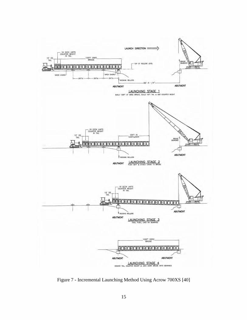
15

Figure 7 - Incremental Launching Method Using Acrow 700XS [40]

16

Advantages of Prefabricated Modular Temporary Bridge Design;

Relatively long spans of up to 125’ can be achieved with this system [39].

The ability to disassemble the span and reuse the material for other projects [40].

The ability to add and subtract panels allows for flexibility in span lengths.

Design allows for a greater clearance for roadway underpasses than could be

achieved with beam spans or girders in most cases.

Maximum span length allows for possibility to use as a jump span while

commencing prep work for a permanent structure.

Stock material available for purchase or rent on short notice.

Ability to use ILM for longer spans makes on-track construction easier where

access proves to be an issue.

Disadvantages of Prefabricated Modular Temporary Bridge Design;

Clearance between modular panels can be limiting for certain types of rail traffic.

Not all span lengths can be achieved using stock material.

Assembly times of as much as 10 days [39] could prove to be costly in emergency

situations.

Skewed substructure would require a detailed design for each case [40].

It is clear that the alternatives outlined in this chapter represent viable solutions to the

problem of service outages due to severe impacts to railway bridge infrastructure.

However an examination of the disadvantages posed by the use of each system shows

17

that additional approaches could prove valuable to service the use cases that the proposed

alternatives cannot achieve. It is obvious that the SSPM utilizing available material

would be ideal for situations where available material matched well with existing

geometry in a way that would allow the permanent replacement of the bridge in a short

period of time. The modular temporary span method would work well in situations

where the engineer is faced with damage to a long span over a major road or waterway

where placing temporary bents is not an option. In between these scenarios there is a

need for a span of up to 55’ (a large percentage of low clearance bridges fall into this

range) that can accommodate skewed substructure geometry and be erected in the field in

a minimum amount of time. Utilizing an emergency steel span made from a kit of parts

held in strategic locations throughout the railway system and constructed using field

welds could achieve this goal and would mean that in situations like the one shown in

Figure 1, train traffic could be restored very quickly. Instead of days or weeks that it

might take to restore the route using alternative methods it would be possible in most

cases to restore service in less than 1 day.

18

Chapter 2

Design of Temporary Structure

The temporary structure was designed with the express purpose of allowing the

railroad a quick, safe and flexible solution to the problem of span failures due to vehicle

impacts. The expected short duration of the span’s service allowed for the use of field

welded connections within the tension zone of diaphragms and stiffener plates that would

be unusual in a permanent structure. Serviceability requirements regarding the maximum

deflection were reduced from the recommended L/640 in the AREMA design manual and

taken per internal emergency response guidelines as;

𝛿𝑚𝑎𝑥 =𝐿

460

(Equation 1)

In all other ways the temporary span was designed in accordance with the codes

outlined in the 2013 edition of the AREMA Manual for Railway Engineering, Volume 2.

Some of the parameters used to define the scope of the design are listed as follows;

Simple Span

W36 rolled beams (based on average necessary clearance requirements)

Steel yield strength of Fy=50 ksi (ASTM A572 Gr. 50)

4 beams per track

19

Designed to withstand Cooper’s E-65 loading

Full diesel impact considered

Span capable of supporting timber ballast deck with 8” of ballast

σmax=.55Fy

Maximum degree of curvature to be considered as 2 degrees

Maximum allowable speed of rail traffic to be considered as 45 mph

The Cooper E loading that was used in the design of this temporary span, as well as

most modern railway bridges, is based on two 2-8-0 Consolidation-type steam

locomotives with an infinite number of railcars represented by a uniformly distributive

load (see Figure 8 and Figure 9) [7] [1]. This standard was first proposed in 1894 by

Theodore Cooper to the American Society of Civil Engineers as a load pattern that would

accurately mimic the controlling forces exerted on bridges from railway traffic at that

time. The loading system is set up as scalable with the original magnitude of the heaviest

axles considered in the proposal to the ASCE by Cooper in 1894 set to E-10 and most

permanent modern railway bridges designed for E-80. The Cooper’s E loading seems to

be outdated, especially in terms of the steam locomotive geometry, but with the ever

changing and varied geometries seen in modern use the Cooper’s loading has proven to

be a good (conservative) approximation of the maximum stresses experienced by modern

structures under load [2] (*Figure 31 and Figure 32 in the section on live loads illustrate

how Cooper’s E-80 load is conservative for maximum stresses in most cases).

20

Figure 8 - 2-8-0 Consolidation-type Locomotive - Basis for Cooper's E loading [8]

Figure 9 - Diagram of Cooper's E-80 Loading for Modern Railway Bridges [1]

Sections 2.1 through 2.7 outline the results from an extensive design and analysis

performed to determine the optimum span geometry for the emergency structure. The

21

beams were sized for maximum Cooper E-65 forces on a 55 foot configuration. The

entire design process included a detailed cost analysis, logistics study and field action

plan that were decided to be outside the scope of this study. Figure 10 shows the basic

plan of the temporary span.

Figure 10 - Plan of Temporary Span

The design analysis results presented in the following sections are valid for an

ASTM A572 steel beam span consisting of 4~W36 X 262 rolled I beams on track curves

not to exceed 2 degrees and speeds not to exceed 45 mph. Furthermore the design

stipulates that the span shall not be utilized in cases where the substructure skew is

22

greater than 30 degrees. For details on placement of stiffeners and diaphragms please

examine Figure 10.

2.1 Dead Load (E-65)

The calculation of the dead load for most railway applications can typically be

estimated with a reasonable degree of accuracy due to the mostly standardized materials

used. For the purposes of design for the temporary span the following items were

considered; the self-weight of the beams, diaphragms, stiffener plates, hardware, rails,

plates, ballast and timber. While the calculation of the dead load included the weight of

the ballast and timber that would be typical in a ballast deck application it is important to

note that the dynamic impact force reduction allowed by AREMA of 10% was not used

due to the unknown nature of the future dead load on the span. This 10% reduction

assumes a substantial dampening effect occurs between the ballast and the span and

would have been inappropriate for an open deck. This assumption should prove to be

conservative for the dead load capacity of the temporary span.

For ordinary steel railway bridges the dead load component is often a small

percentage of the total load [2]. This is due to the fact that the live load component

(locomotive/railcars) of the total load is much greater than is typical in most other

structural design problems. Figure 11 and Figure 12 show the values for moment and

shear due to dead load at intervals up to mid-span (*Span is symmetrical). The line

labeled “Girder” in Figure 11 and Figure 12 represents the moment and shear reaction

due to dead load while SDL denotes the reactions due to the sum of all the dead loads.

23

Figure 11 - Moment in Beams Due to Self-Weight and Superimposed Dead Load

Figure 12 - Shear in Beams Due to Self-Weight and Super Imposed Dead Load

0

100

200

300

400

500

600

700

0.00 5.00 10.00 15.00 20.00 25.00 30.00

M (

k-ft

/rai

l)

Beam Length (ft.)

Girder

SDL

14.15

47.95

0

10

20

30

40

50

60

0.00 5.00 10.00 15.00 20.00 25.00 30.00

V (

kip

/rai

l)

Beam Length (ft.)

Girder

SDL

24

2.2 Live Load (E-65)

The design live load of most modern railway structures is based on the Cooper E

loading as previously discussed. Utilizing this design loading as a standard for the

industry allows for a more simplified standard approach for design engineers while still

providing a loading system that is conservative in most cases. It is of particular

importance that the live load be conservative or at least accurate at predicting actual load

values because the live load represents a much greater percentage of total load than any

of the other load categories prescribed by AREMA. The live load considered for the

temporary span was Cooper’s E-65 loading whose geometry is shown in Figure 9. Figure

13 and Figure 14 show the shear and moment induced by E-65 loading on the temporary

span.

Figure 13 - Moment Induced by Cooper's E-65 Load

0

500

1,000

1,500

2,000

0.00 5.00 10.00 15.00 20.00 25.00 30.00

MLL

(k-

ft/r

ail)

Beam Length (ft.)

25

Figure 14 - Shear Induced by Cooper's E-65 Load

2.3 Combined Factored Loads (E-65)

In addition to the dead load and live load a number of other design loads were

considered during the design of the temporary span as outlined by AREMA. The

fundamental basics of these additional loads will be covered more extensively in Section

3.1.3 through 3.1.5 and include impact load, longitudinal load and centrifugal load. Of

all the additional loads it is impact that plays the most important part in increasing the

design stresses in the structure. As discussed briefly in Section 2.1 the full diesel impact

(no 10% reduction) on the span was considered in addition to the weight of the ballast

deck thus ensuring a conservative result for whatever deck type is used on the temporary

span. Figure 15 and Figure 16 show the moment and shear values for the temporary span

due to the combined loads (including dead and live load) plus full impact.

149.32

0

20

40

60

80

100

120

140

160

0.00 5.00 10.00 15.00 20.00 25.00 30.00

VLL

(ki

p/r

ail)

Beam Length (ft.)

26

Figure 15 - Moment Due to Total Combined Loads + Impact

Figure 16 - Shear Due to Total Combined Loads + Impact

2.4 Tension Stress Check

Figure 17 shows the calculated tensile stress in the extreme fiber of the W36x262

beam plotted against the AREMA allowable stress for steel members of [1],

𝜎𝑎𝑙𝑙 = .55𝐹𝑦 (Equation 2)

0

500

1,000

1,500

2,000

2,500

0.00 5.00 10.00 15.00 20.00 25.00 30.00

Mu

(k-

ft/g

ird

er)

Beam Length (ft.)

163.58

0

50

100

150

200

0.00 5.00 10.00 15.00 20.00 25.00 30.00

Vu

(ki

p/g

ird

er)

Beam Length (ft.)

27

Where,

𝜎𝑎𝑙𝑙= Allowable stress = 27.5 for ASTM A572 Gr. 50 steel.

𝐹𝑦= Material yield strength = 50 ksi for ASTM A572 Gr. 50 steel.

Examination of Figure 17 shows the temporary span is sufficient in tension per

AREMA guidelines for E-65 loading.

Figure 17 - Tension Stresses vs Allowable Stress

2.5 Compression Stress Check

Figure 18 shows the calculated compressive stress in the extreme fiber of the

W36x262 beam plotted against the AREMA allowable stress for steel members shown in

(Equation 2). This highlights the absolute maximum stress that is allowed in the span per

AREMA guidelines.

0

5

10

15

20

25

30

0.00 5.00 10.00 15.00 20.00 25.00 30.00

Stre

ss, f

(ks

i)

Beam Length (ft.)

Tension Stress

Allowable Stress

28

In order to account for the maximum distance of diaphragms for the purposes of

preventing lateral torsional buckling the following equation was used to account for a

maximum allowable compression stress (Fcall) as a function of the unbraced length and

the radius of gyration of the member’s weak axis [1];

𝐹𝑐𝑎𝑙𝑙 =. 55𝐹𝑦 −. 55𝐹𝑦

2

6.3𝜋2𝐸(

𝑙

𝑟𝑦)

2

< .55𝐹𝑦 (Equation 3)

Where,

𝑙 = Unbraced length

𝑟𝑦 = minimum radius of gyration of the compression flange

Application of (Equation 3) in conjunction with special provisions in the AREMA

Manual show that a maximum spacing of 11’-0” center to center is appropriate for the

diaphragm system.

29

Figure 18 - Compressive Stresses vs Allowable Stress

2.6 Shear Stress Check

Figure 19 shows the calculated shear stress in the web of the W36x262 beam

plotted against the AREMA allowable sheer stress (𝜏𝑎𝑙𝑙) for steel members shown by the

following equation [1];

𝜏𝑎𝑙𝑙 = .35𝐹𝑦 (Equation 4)

This highlights the absolute maximum shear stress that is allowed in the web of

the rolled beam section per AREMA guidelines.

0

5

10

15

20

25

30

0.00 5.00 10.00 15.00 20.00 25.00 30.00

Stre

ss, f

(ks

i)

Beam Length (ft.)

Compression Stress

Allowable Stress

30

Figure 19 - Shear Stresses vs Allowable Stresses

2.7 Initial Overview of Fatigue for Temporary Span

The above results show that the span geometry as outlined in the design is adequate to

meet service requirements in the short term. Even though it is shown in later sections of

this research that Cooper’s loads do not necessarily accurately reflect fatigue loading in

steel railway bridges it is still useful to consider fatigue effects induced by design loads

as a validation for further research into the subject. The AREMA design manual offers

guidance on fatigue design by classifying connection details into categories whose

allowable stress ranges (ΔSR) have been determined by empirical analysis [1]. An

inspection of the stiffener plate-to-flange and stiffener plate-to-web connections indicates

that these connections fall into fatigue category C’1 (see Figure 20).

1 AREMA designates fatigue categories for common construction details and includes guidance on the maximum allowable stress range for each category. If a detail covered by a fatigue category experiences a stress range within this limit it will be able to sustain more than 2 million cycles and is considered to have infinite fatigue life [1].

0

5

10

15

20

0.00 5.00 10.00 15.00 20.00 25.00 30.00

Stre

ss, f

(ks

i)

Beam Length (ft.)

Shear Stress

Allowable Stress

31

In order to expedite the initial fatigue analysis only in-plane forces were considered in

the rolled I-beams. Forces induced by differential deflection of the beams and transferred

through the diaphragms were not considered. The effective stress range of incremental

sections along the span was calculated and compared with the allowable stress ranges for

the fatigue categories outlined in the AREMA manual to determine which category

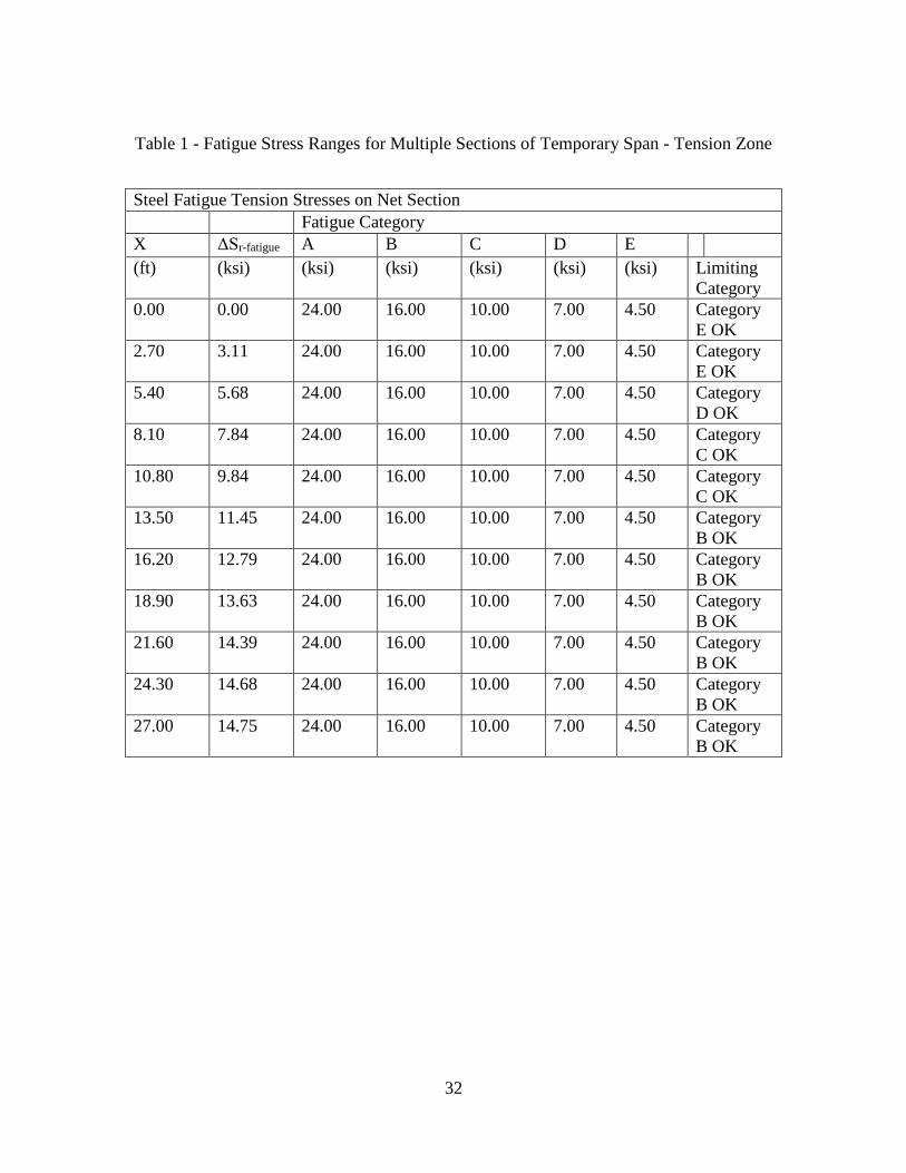
would control at that section (see Table 1). The manual stipulates that stress ranges that

fall within the specified stress range for the appropriate category will be adequate for

over 2 million cycles when subjected to continuous unit trains with axle loads not

exceeding 80,000 pounds on spans less than 100 feet [1]. Table 2 shows the calculated

stress range at the location of the controlling welded stiffener. Investigation of Table 2

shows that the stiffener-to-beam connection exceeds its controlling category’s allowable

stress range (C’) by almost 2.43 ksi. In Table 2 allowable and actual stresses have been

highlighted in red for clarity.

32

Table 1 - Fatigue Stress Ranges for Multiple Sections of Temporary Span - Tension Zone

Steel Fatigue Tension Stresses on Net Section

Fatigue Category

X ΔSr-fatigue A B C D E

(ft) (ksi) (ksi) (ksi) (ksi) (ksi) (ksi) Limiting

Category

0.00 0.00 24.00 16.00 10.00 7.00 4.50 Category

E OK

2.70 3.11 24.00 16.00 10.00 7.00 4.50 Category

E OK

5.40 5.68 24.00 16.00 10.00 7.00 4.50 Category

D OK

8.10 7.84 24.00 16.00 10.00 7.00 4.50 Category

C OK

10.80 9.84 24.00 16.00 10.00 7.00 4.50 Category

C OK

13.50 11.45 24.00 16.00 10.00 7.00 4.50 Category

B OK

16.20 12.79 24.00 16.00 10.00 7.00 4.50 Category

B OK

18.90 13.63 24.00 16.00 10.00 7.00 4.50 Category

B OK

21.60 14.39 24.00 16.00 10.00 7.00 4.50 Category

B OK

24.30 14.68 24.00 16.00 10.00 7.00 4.50 Category

B OK

27.00 14.75 24.00 16.00 10.00 7.00 4.50 Category

B OK

33

Table 2 - Fatigue Detail For Critical Connection 55' Span

Steel Fatigue Tension Stresses on Net Section, At Welded Attachment

Fatigue Category

X ffatigue A B C’ D E

(ft) (ksi) (ksi) (ksi) (ksi) (ksi) (ksi) Limiting

Category

22.00 14.43 24.00 16.00 12.00 7.00 4.50 Category

B OK

Figure 20 - AREMA Fatigue Category C' [1]

The results of the initial analysis indicate that the service life of the span will

likely be less than 2 million cycles. Since the span is designed as a temporary measure

with a limited service life this limitation may not prove to be an issue. However, now

that it has been shown that the design of fatigue prone connections in the temporary span

do not conform to the recommended practices accepted by the industry it becomes

necessary to investigate the fatigue damage accumulated at these connections further in

order to determine a safe limit to the emergency span’s service life.

34

2.7.1 Use of Finite Element Analysis to Achieve Meaningful Results

Traditionally, fatigue analysis has been a mostly test based endeavor and therefore

has been very costly as well as time consuming and labor intensive. A purely test based

fatigue analysis is also problematic in that it does not allow for the flexibility to slightly

change certain design parameters in order to maximize design efficiency. By utilizing a

finite element analysis approach to the problem of fatigue testing for welded connections

on a temporary railway span it is possible to get a similarly useful result without the

drawbacks associated with traditional lab testing.

All structural analysis whether lab based or FEM requires at least three

independent criteria; material, loading and geometry. Material is what the structure is

made out of and it is important to understand each material’s unique properties in order to

understand how that material will resist loading. The materials used in the construction

of the temporary railway span include ASTM A572 Structural Steel for the beam spans

and diaphragms, Southern Yellow Pine for bridge ties, as well as ASTM A307 Hook

bolts and hardware. The material properties being considered are independent of the

method used to test them. This means that in theory as long as quality control procedures

have been adequately administered on physical members their properties should be

identical or within negligible tolerance compared with material properties used in an

FEM analysis. The benefit of using an FEM analysis is that these properties can be

changed and manipulated in order to achieve maximum efficiency.

35

Loading represents the forces that the structure will be subjected to. In the case of

the temporary beam span these include the structures self-weight as well as external loads

such as the locomotive, rail cars, wind and seismic loads. For the benefit of a finite

element analysis the loads that the structure being analyzed is subjected to can be

characterized into the following cases; dead load, live load, impact load, wind load,

centrifugal forces, longitudinal load and lateral forces. These forces can be carefully

calibrated either through mathematical models or from empirical observation to closely

mimic real world loading conditions.

Geometry represents the shape of the structure. It is intuitively understood that

different shapes will be more efficient than others at resisting loads. For instance, it is

understood that a piece of paper that is rolled into a cylinder will be much more effective

as a column supporting a load from above that the same piece of paper stood up on its

side. While the concept is easily understood, achieving the most efficient geometry in a

given structure can be a difficult task. One of the major drawbacks of using physical

prototypes of members to conduct lab tests (including fatigue analysis) is that in order to

test a different geometry it would be necessary to construct an entirely new prototype in

most cases. FEM modeling allows for a much greater flexibility in terms of geometry by

allowing the user to alter or completely change geometries being tested with relatively

minimum effort and without the constraining costs of building new physical models.

36

Figure 21 helps to illustrate schematically how FEM modeling is leveraged in this

research as a means to achieve similarly useful objectives compared with traditional lab-

test based analysis

For FEM analysis

When considering the problems imposed by the analysis of the temporary railway

span it is easy to see how FEM modeling is by far the most attractive option. The entire

premise of the structure is that it will only be used in the event of an emergency. This

structure is never intended to be used unless absolutely necessary and does not utilize the

traditional construction methods that have been proven safe and effective for normal

railway use. The fatigue vulnerable welded connections in particular can be seen as case

and point. Since there are no similar connections currently in service among class I2

2 The designation of a Class I railroad is defined by the Surface Transportation Board as a railroad having annual operating revenues of $250 million or more after adjusting for inflation using the Railroad Freight Price Index developed by the Bureau of Labor Statistics. As of 2011 this figure stood at $433.2 million.

Material Loading

Geometry (Physical vs FEM)

Analysis

Results

Figure 21 - FEM vs Physical Modelling

37

railroad infrastructure that are known to this author a systematic study of the fatigue life

of such a connection over time in the field is impossible. By using an FEM analysis to

predict the effective fatigue life of these connections the railroad industry can be given a

reasonably accurate prediction of the structures useful lifespan in a timely and cost

effective way without the need to compromise safety which has always been the

industries’ top priority.

There are currently 7 class 1 freight railroads operating in the United States including; BNSF Railway, Union Pacific Railway, CSX Railway, Canadian National Railway, Canadian Pacific Railway, Norfolk Southern Railway and Kansas City Southern Railway. Together these Class I railroads make up the vast majority of railway track and infrastructure in the United States.

38

Chapter 3

Modelling of Temporary Span in RISA 3D

RISA 3D was used to model the entire temporary span in order to predict the

applied forces necessary for a fatigue analysis. RISA 3D was chosen as the best

candidate for the modelling of the structure for a number of important reasons. Chief

among these reasons was the intuitive nature of the user interface that made modelling

the temporary structure in multiple configurations relatively quick. The moving load

feature available in RISA 3D was another factor that made its use an appealing option as

load patterns could be set and then simply scaled up and down to simulate lighter loads

(286K and 315K railcars are a good example). Some of the drawback to using this

software is the inability to customize surface and part interaction or to model complex

local geometries. That is why it was decided that for the purposes of this research that

RISA 3D would be used to quickly test loads and span geometries to ascertain the

suitability of those variables for further analysis. Once a controlling combination of

loads and geometries were obtained it would then be possible to apply the forces and

conditions predicted by the RISA analysis to a more detailed model of the complex

geometry of the critical connection.

One of the factors often left out in the design of railway bridges is the effect that

the rail and ties will have on the distribution of loads to the superstructure. It is common

practice to consider the Cooper load outlined previously as acting directly on the load

39

supporting element as a concentrated force. However, anyone with a background in

engineering would recognize that the ties and especially the rail are both serving to

distribute the load over a greater area. This is particularly true of longitudinal forces, of

which a significant percentage would be transferred by the rail and not affect the

substructure or superstructure of a relatively short bridge. While a complex discussion of

how force distribution affects longitudinal forces is outside the scope of this research the

effects of distribution of vertical and transverse forces will be captured by the finite

element model as long as proper detailing of the model is achieved. In order to achieve

this objective the rail was modelled as an arbitrary rectangle but assigned the section

properties of 136# Class 1 rail which is one of the most common rail types on North

American class 1 railway mainlines. Figure 22 shows the section properties that were

assigned to the rail in the FEM model.

40

Area (in2) 13.32

Section Modulus – Head

(in3)

23.78

Section Modulus – Base

(in3)

28.3

Moment of Inertia (in4) 93.7

Figure 22 - 136# Rail Properties

Figure 23 - 136# Rail Fastened with Pandrol

Plates

Since all forces with the exception of wind or seismic forces act on the structure

through the rail it is important that the rail-to-tie and tie-to-superstructure connection be

modelled as accurate to real world conditions as possible. This created somewhat of a

challenge in RISA 3D as the basic functionality is set up to connect members at nodes

that are always located at the centroid of the member. In order to facilitate a “stacked”

geometry where members interact from their respective surfaces it was necessary to

utilize rigid links. These links were modeled with a high stiffness and zero density so as

41

not to interfere with dead load calculations. In the case of the emergency span modeled

in RISA 3D the interactions were modelled using rigid links with end conditions treated

as either fully fixed for mostly rigid connections or pinned for moment released

connections.

The vast majority of rail-to-tie connections on bridges are made using Pandrol tie

plates that act as “elastic fasteners” and hold the rail, plate, and tie together in a mostly

rigid manner. Figure 23 shows a picture of a bridge deck that utilizes Pandrol plates for

rail-to-tie connections. These connections were considered capable of imparting moment

to the ties and therefore a fully fixed rigid link like the example shown in Figure 24 were

used to model the interactions. The tie-to-superstructure link is almost always made

using either HCP clips or hook bolts like the one shown in Figure 25. It is obvious that

this type of connection would be able to resist translation in the vertical (Y) and lateral

(Z) direction but would provide negligible moment capacity. Therefore the tie-to-

superstructure link was modelled as moment released. This has the added benefit of

being conservative in terms of the stresses in the beams as it lowers the stiffness of the

system.

42

Figure 24 - Rigid Link for Rail-to-Tie Connection

Figure 25 - Typical Hook Bolt

3.1 Forces

Once the FEM models for each span were accurately modeled in a way that most

closely resembled real world connections it was important to ensure that the appropriate

loads were then applied in such a way that produced the stresses and forces within the

structure that correspond to the actual response. The determination of appropriate

loading is a function of intense research by academics in the railway engineering field as

well as a proper application of design constraints. External forces were applied at

increments along the structure and solved statically with member forces and stress cycles

determined from the results. In order to account for the dynamic elements of the moving

train loads a series of additional loads were considered to replace such effects on the

structure. This method of using static solutions to model dynamic behavior has been

43

shown through research conducted by the American Association of Railroads to be

accurate or conservative at predicting fatigue life of railway structures [1].

3.1.1 Dead Load

The dead load of the emergency span consists of the weight of the structure itself in

conjunction with any permanent fixtures to the superstructure such as hardware or ties.

The American Railway Engineering and Maintenance of Way association provides

guidance on appropriate dead load values (See Table 3) [1]. The dead load considered

for the FEM analysis is as follows.

4 ~ W36 x 262 ASTM A572 steel beams

2’ x 2’-6” x ½” ASTM A572 steel diaphragm plates (varying quantities)

7” x 2’-10” x ½” ASTM A572 steel stiffener plans (varying quantities)

10” x 10” Southern yellow pine bridge ties

136# rail (Figure 22)

44

Table 3 - Dead Loads on Steel Bridges

Dead Loads on Steel Bridges

Type Pounds per Cubic Foot

Steel 490

Concrete 150

Sand, gravel and ballast 120

Asphalt-mastic and bituminous macadam 150

Granite 170

Paving Bricks 150

Timber 60

Track rail, fastenings and guard rails 200 Pounds per Linear

Foot

*Information from the American Railway Engineering and Maintenance of Way

Association, Manual for Railway Engineering, Chapter 15.

3.1.2 Live Load

The determination of live loads for railway bridges can be somewhat complex due

to the variability of locomotives and equipment used on railroads. The loads that existing

railway infrastructure is expected to support has traditionally increased over time and the

implementation of heavier loads has accelerated dramatically in the last 25 years [3].

This means that in the future the emergency beam span may be asked to support loads

that it was not designed for. A railway engineer in the future that is confronted with a

bridge failure and has the emergency material on hand may make a determination to

allow heavier loads on the span. This is not an unreasonable decision considering that the

allowable stress in the steel span is a very conservative .55fy. However, such a decision

must be made with an understanding of how the critical connections will behave under

these heavier loads in terms of it’s fatigue life. In order to best meet this need this

research paper has considered not only current standard loads but also future potential

loads.

45

Some of the heaviest locomotives in the North American railway industry can

reach up to 435,000 pounds and generally consist of 2 ~ three axle sets spaced roughly

45.62 to 54.63’ apart (see Figure 26) [2]. Locomotives are typically found in sets of two

at the front and rear of a train. Many foreign railroads already employ much larger and

heavier locomotives in their fleets than do American and Canadian railroads and it is not

unreasonable to assume that the North American railway industry will continue to see

increases in the gross weight of their locomotives in the future [3]. The stresses induced

by the locomotive are one of the primary contributing factors in the accumulation of

damage to the critical connections in the emergency span.

Figure 26 - Typical 435K Railway Locomotive

Prior to the introduction of 263 kip rail cars in the 1960s the primary concern for

fatigue damage to railway bridges came from the locomotive only. With the introduction

of the heavier 263 kip gross weight rail cars the number of cycles accumulated in some

bridge members increased by a factor of 60 [1] (* Part 9.1.3.13 commentary). The

resulting damage to railway structures was severe. In the late 80s and early 90s the

Association of American Railroads conducted a research study known as the Heavy Axle

Load Research Program (HAL) into to the viability of using 286 kip gross vehicle weight

46

cars on existing railway infrastructure. The study concluded that the added strain on the

railway infrastructure, and particularly bridges, and the associated maintenance cost and

shorter lifespans were offset by the economic benefits of carrying heavier rail cars

including those up to 315,000 pounds. This gave the industry incentive to increase loads

despite the increased damage that would accumulate on railway bridges [4]. While the

industry has yet to fully adopt the 315 kip rail cars as a standard for the majority of traffic

the conversion to 286 kip cars is undeniable. 90% of newly acquired rail cars are rated

for at least 286 kip loads and almost 100% of coal traffic and 40% of general freight

traffic is moved in 286 kip or higher cars [3]. One segment of rail traffic where 315K

railcars are being quickly adopted is on the so called “Coal Corridors”. Therefore, this

research assumed that the conversion to the heavier 315K railcars will continue and used

the weight and configuration of one of the most common types of 315K cars in the FEA

analysis. Figure 27 illustrates the geometry of a typical 315 kip rail car.

Figure 27 - Typical 315K Rail Car

47

For the purposes the FEM analysis the loads and load patterns of the 435 kip

locomotive and the 286 or 315 kip railcar were broken down into individual vertical loads

acting on each rail from each wheel. Together these elements make up the live load that

was applied to the FEM Model. Figure 28 shows an example of the force distribution

conventions used for the model. This figure illustrates the load pattern for 1~435K

locomotive and 2~315K railcars. Note that even though the locomotive is heavier than

the railcars it exhibits less force than the railcar per axle/wheel. A cross section of the

span is shown in Figure 29 that illustrates the loading from one single axle of a 315K

railcar on the temporary structure. Utilizing the moving load capability of RISA 3D the

live load as well as all other moving loads were built into the program and stepped in

increments of 1 inch and solved statically to determine stresses and forces at multiple

points. Although at first glance a static solution might seem to be inadequate for the

purposes of modelling stresses due to train loads it has been shown through extensive

research [1] [5] that the fatigue behavior of steel railway bridges can be accurately

modelled when corrected for dynamic behavior with appropriate static loads that will be

discussed in the following sections of this research. Figure 30 shows how live loads were

entered into the FEM model in order to quickly calculate the stresses and forces in the

structure at multiple points.

48

Figure 28 - Force Distribution for Locomotive and 2 Railcars

Figure 29 - Live Load from 315K Railcar

Figure 30 - RISA 3D Interface Showing

Live Load Entry

In practice as well as in the initial phase of the FEM model it is considered that

each train consists of 2 ~ 435K locomotives at the front, 110 railcars of either 286K or

315K gross weight and 2 additional locomotives in the rear. Justification for these

figures is taken from the American Association of Railroads Factbook [6].

49

It is important to note that the Cooper E loading that is prescribed in the AREMA

manual for the design of steel railway bridges and was used to design the emergency span

has been shown to be inaccurate at predicting the fatigue behavior of steel structures,

particularly short spans [1] [2]. This fact can be seen clearly from examination of Figure

31 and Figure 32. It is obvious that the Cooper loads would be insufficient at predicting

the fatigue behavior of the span under load from railcars because the constant distributed

load used to model railcars would essentially produce no effective stress range (ΔSre).

This discrepancy is explained by the fact that when the Copper’s E loading was accepted

as a standard for the railway industry in the early-20th century the use of railcars with

sufficient weight to induce fatigue damage to structures had yet to see wide adoption [1]

(Part 9 commentary). Furthermore it can be observed on short spans that the Cooper load

underestimates the number of fatigue cycles due to the locomotive significantly and that

for longer spans it is over conservative in terms of stress magnitude [2].

Figure 31 - E80 vs Actual Load - Flexure

25' Span [2]

Figure 32 - E80 vs Actual Load - Flexure

60' Span [2]

50

It is for this reason that this research has concentrated on developing a fatigue

analysis based on real world loads.

3.1.3 Impact Load

The amplification of loads due to impact is perhaps one of the most complicated

and least understood aspects of design and analysis of railway structures. The two major

impact factors that were considered during the analysis of the temporary span were

vertical effects due to superstructure-vehicle interaction and the amplification of vertical

wheel loads due to lateral rocking effects.

The determination of the impact factor due to rocking effect is fairly straight

forward. Locomotives and railcars will tend to rock or sway due to track conditions,

wind, super-elevation transition and stiffness variance in suspension systems causing

vertical amplification of the wheel loads. Numerous test conducted by AREA in 1949

and 1955 have demonstrated that the rocking effect is independent of the velocity of the

train [9]. AREMA has recommended that rocking effect be calculated by the following

simple equation [1];

𝑅𝐸 =100

𝑆

(Equation 5)

Where,

RE = Rocking effect (as a percentage of live load)

51

S = Distance between centerline of rails (feet)

For most main line track on class 1 railways in North America the distance

between rails can be considered approximately 5 feet meaning that the rocking effect will

generally be taken as 20% of live load.

The vertical effects of superstructure-vehicle interaction are much more complex

to determine. Superstructure vibration is induced by the train as it traverses the bridge.

For bridges with relatively short spans in comparison to the train geometry such as the

temporary span it is possible to consider the effects of concentrated moving loads to

approximate an impact factor [1]. A dynamic impact factor (Ivs) can be determined

classically as a ratio of dynamic deflection (yd) to static deflection (ys). Assuming small

deformation and considering internal damping negligible in comparison to the external

damping the partial differential equation of motion can be expressed as [2];

𝑝(𝑥, 𝑡) = 𝐸𝐼𝜕4𝑦𝑑(𝑥, 𝑡)

𝜕𝑥4+ 𝑚

𝜕2𝑦𝑑(𝑥, 𝑡)

𝜕𝑡2+ 𝑐

𝜕𝑦𝑑(𝑥, 𝑡)

𝜕𝑡

(Equation 6)

Where,

yd(x,t) = Dynamic deflection at distance x and time t

EI = Flexural stiffness of the structure

m = mass of the superstructure per unit length

52

c = viscous damping coefficient of the superstructure

p(x,t) = Moving load on bridge at distance x and time t

Assuming that the temporary span is sufficiently short for a dynamic response to

be approximated by a concentrated load;

𝑝(𝑥, 𝑡) = 𝛿(𝜉)𝑃 (Equation 7)

Where,

δ(ξ) = The Dirac Delta function and physically represents the density of the idealized

point mass at ξ = x-Vt

P = Concentrated force.

Considering the d’Alembert’s principle of inertial effects the concentrated load

can be taken as [2];

𝑃 = (𝐹(𝑡) + 𝑚𝑣𝑔) − 𝑚𝑣[𝑔 − (𝑑2𝑦𝑑(𝑉𝑡, 𝑡)

𝑑𝑡2)]

(Equation 8)

Where,

F(t) = The dynamic force due to concentrated moving load such as vehicle suspension

53

mv = The mass of the concentrated force

g = The acceleration due to gravity

Combining (Equation 6), (Equation 7) and (Equation 8) yields.

𝛿(𝑥 − 𝑉𝑡)(𝐹(𝑡) + 𝑚𝑣𝑔) − 𝑚𝑣 [𝑔 − (𝑑2𝑦𝑑(𝑉𝑡, 𝑡)

𝑑𝑡2)]

= 𝐸𝐼𝜕4𝑦𝑑(𝑥, 𝑡)

𝜕𝑥4+ 𝑚

𝜕2𝑦𝑑(𝑥, 𝑡)

𝜕𝑡2+ 𝑐

𝜕𝑦𝑑(𝑥, 𝑡)

𝜕𝑡

(Equation 9)

In order to simplify (Equation 9) the dynamic load due to suspension will be

neglected due to the relatively slow 45 mph speed restriction on the temporary span.

Despite this simplification the solution to the above equation is still quite complex. A

complete explanation of the solution for (Equation 9) can be found in Dynamics of

Railway Bridges by Ladislav Fryba [10]. Using the transformative techniques described

by Dr. Fryba yields the following solution for dynamic displacement.

54

𝑦𝑑(𝑥, 𝑡) =2𝑚𝑣𝑔𝐿3

𝜋4𝐸𝐼∑

1

𝑖2[𝑖2 (𝑖2 − (𝜔𝜔1

)2

)2

+ 4(𝜔𝜔1

)2

(𝜔𝜔1

)2

]

∞

𝑖=1[

𝑖2 [𝑖2

− (𝜔

𝜔1)2

] 𝑠𝑖𝑛𝑖𝜔𝑡

−𝑖 (

𝜔𝜔1

) [𝑖2 (𝑖2 − (𝜔𝜔1

)2

) − 2 (𝜔𝜔1

)2

]

√𝑖4 − (𝜔𝜔1

)2

𝑒−𝜔𝑡𝑠𝑖𝑛√𝜔𝑖2 − 𝜔𝑐

2𝑡

− 2𝑖 (𝜔

𝜔1) (

𝜔

𝜔𝑐) (𝑐𝑜𝑠𝑖𝜔𝑡 − 𝑒−𝜔𝑐𝑡𝑥𝑐𝑜𝑠√𝜔𝑖

2 − 𝜔𝑐2𝑡)

]

𝑠𝑖𝑛𝑖𝜋𝑥

𝐿

(Equation

10)

Where,

𝜔1 =𝜋2

𝐿2√

𝐸𝐼

𝑚 is the fundamental frequency of an unloaded simply supported beam [2]

[10]

𝜔 =𝜋𝑉

𝐿 is the forcing frequency of p(x,t)

In the case of the temporary structure it can be assumed that ωc < 1 and neglected

[2]. Furthermore, previous equations can be simplified by neglecting the damping and

setting c=2mωc=0. Assuming a sinusoidal shape function as prescribed by Anil Chopra

in Dynamics of Structures [11] yields the following equation for mid-span deflection.

55

𝑦𝑑(𝑚𝑖𝑑𝑠𝑝𝑎𝑛, 𝑡) =2𝑃

𝑚𝐿 [𝜔12 − (

𝜋𝑉𝐿 )

2

]

(𝑠𝑖𝑛𝜋𝑉𝑡

𝐿−

𝜋𝑉

𝜔1𝐿𝑠𝑖𝑛𝜔1𝑡)

(Equation 11)

Figure 33 shows the calculated dynamic deflection at mid-span of the 55 foot

tangent substructure emergency span configuration using (Equation 11) vs the static

deflection at mid-span.

Figure 33 - Dynamic Deflection of Temporary Span

The calculated maximum deflection due to dynamic interaction of a 315K railcar

and superstructure interaction on inspection of Figure 33 is 1.039”. The deflection due to

static forces is also shown in Figure 33 and is calculated as follows;

0

0.2

0.4

0.6

0.8

1

1.2

0 0.1 0.2 0.3 0.4 0.5 0.6 0.7

De

fle

cto

tio

n 3

15

K C

ar (

inch

es)

Time (seconds)

Dynamic Deflection vs Static Deflection Temporary Span (Mid-Span 55')

yd(x,t)

ys

56

𝑦𝑠 =𝑃𝐿3

48𝐸𝐼= .908"

(Equation 12)

As stated previously the impact factor due to vehicle-superstructure interaction

can be classically solved as a ratio of dynamic to static deflection.

𝐼𝑣𝑠 =𝑦𝑑

𝑦𝑠=

1.039

. 908= 1.145

(Equation 13)

(Equation 13) indicates that the impact factor due to superstructure-vehicle

interaction is roughly 14.5%. However, due to the simplifying assumptions made in the

formulation of (Equation 11) the final calculated impact factor will likely underestimate

the forces due to impact as experienced by the actual structure significantly. An

understanding of all the characteristics that govern the magnitude of the impact factor of

vehicle-superstructure interaction is important to understanding why the calculated

impact could be significantly undersized. The primary parameters affecting the dynamic

behavior of the emergency beam span are;

Train Speed

Span Length

Track Geometry

Mechanical condition of the train

Live load characteristics of the train

57

Train handling

Bridge supports

Bridge layout

Condition of the track

AREMA recommends a formula for the determination of an appropriate impact

factor based on empirical analysis [1]. On spans less than 80 feet the vertical impact

factor recommended by AREMA is.

𝐼𝑣𝑠 = 40 −3𝐿2

1600

(Equation 14)

For the temporary structure with a length of 55 feet, Ivs = 40 – 3(55)2/1600 =

34.33%. When combined with the effects due to rocking the total impact load for the

temporary structure was taken as Itotal = 34.33+20 = 54.33%. Figure 34 shows how the

impact factor was applied to the FEM model.

Figure 34 - FEM Impact Factor

58

The large discrepancy between the calculated impact factor due to 315K railcars

and the empirical impact factors described in AREMA at first seem incompatible.

However, it must be noted that the AREMA impact factors have a probability of

occurrence of approximately 1%. Even at that low probability of occurrence it is

assumed that a permanent railway structure that is designed for at least 80 years of

service will be subjected to this full impact load multiple times within it service life. For

the purposes of fatigue analysis the AREMA manual allows a reduction in the empirical

impact factor to 35% for beams such as the beam emergency span (Figure 35) [1].

Applying this reduction to the empirical impact value yields an AREMA assumed mean

impact value for the temporary steel span of 12.02%. This is much more in line with the

calculated value of 14.5%.

Figure 35 - Fatigue Impact Load Percentages [1]

However, the reductions assumed in Figure 35 are not appropriate for the

temporary span due to the multiple unknown variables associate with its implementation

such as and the condition and type of track it will be used on as well as the variability of

59

the span length and geometry. Full impact load was used for the FEM analysis in this

study.

3.1.4 Centrifugal Forces

Centrifugal forces are the product of train loads as they travel through a curve in

the track and act through the centroid of the train’s mass in a direction perpendicular to

the direction being travelled. The AREMA design manual recommends that the center of

gravity be taken at a distance 8 feet above the rail situated at an equal distance between

the rails (see Figure 37) [1]. A quick inspection of the geometries of the 435K

locomotive and the 315K rail car shown in Figure 26 and Figure 27 will confirm that this

is a valid recommendation for the geometries being considered for this research study.

The centrifugal force corresponding to each axle load is shown below [2].

𝐶𝐹𝐴 =𝑃𝐴 ∗ 𝑉2

𝑔 ∗ 𝑅

(Equation 15)

Where,

PA = Axle load (kips)

V = Speed of the train (mph)

g = Acceleration due to gravity = 32.174 ft/s/s = 78,972 mph/hr

R = radius of the curve = 5730/D (ft) = 1.085227/D (mi)

60

Converting all variables into units of kips, miles and hours and plugging into

(Equation 15) yields;

𝐶𝐹𝐴 =𝑃𝐴 ∗ 𝑉2 ∗ 𝐷

78,972 ∗ 1.085227

= 0.0000117𝑃𝐴𝑉2𝐷

(Equation 16)

Where,

D = Degree of Curvature

Now consider that during the design of the temporary span it was decided that the

maximum allowable curvature (D) would be limited to 2 degrees and that the maximum

allowable speed as outlined in the section devoted to impact loads would be set to 60

mph. Plugging these values into (Equation 16) and considering the axle load of a typical

315K railcar will give an example of an appropriate centrifugal load as applied at the

center of gravity (see Figure 37).

𝐶𝐹𝐴 = 0.0000117 ∗ 78.75 ∗ 602 ∗ 2 = 6.63 𝑘𝑖𝑝𝑠

In order to apply the centrifugal load to the FEM model in a way that would

simulate the load acting through the center of gravity it was necessary to perform some

simple statics calculations to come up with a series of loads that would have an

equivalent effect on the structure. Figure 36 shows the static solution for the reactions at

the rails for the centrifugal force from 1 axle of a typical 315K railcar. The equivalent

61

loading at the rails (which are the point of load transfer to the structure from the railcar)

to simulate the centrifugal force is equal and opposite of the reactions calculated in the

static solution. Figure 39 shows how these forces are applied to the temporary span.

∑𝑀𝐵 = 0

(6.63)(8)+RAY(-5)=0

=> RAY=10.61 Kips

∑𝐹𝑌 = 0

10.61+RBY=0

=> RBY=-10.61 Kips

∑𝐹𝑋 = 0

RAX+ RAX -6.63=0, RAX= RBX

=> RAX and RBX=3.315 Kips

Figure 36 - Free Body Diagram of Centrifugal Force

62

Figure 37 - Centrifugal Force Applied at Center

of Gravity

Figure 38 - RISA 3D Interface

Showing Centrifugal Forces Entry

Figure 39 - Equivalent Centrifugal Force System on FEM Model

63

3.1.5 Longitudinal Forces

The dynamic forces applied to the emergency beam span in the longitudinal

direction are primarily a product of braking and tractive forces [1] [2]. There have been a

number of changes to the recommendations for the magnitude and placement of the

longitudinal forces within the AREMA manual over the last several decades. By the time

of the 1996 edition of the design manual it was shown through testing conducted by the

AAR that longitudinal forces were in fact as much as 25 times greater than those

recommended in the manual [1] [7]. A precise analysis of the longitudinal effect of train

loads is very complex and continues to be an active field of research within the railway

engineering community. For the purposes of this research the most current

recommendations in the AREMA manual were used and adapted to suit needs of the

FEM analysis.

The 2013 edition of the AREMA MRE was developed for use with the Cooper’s

E80 load and states that the longitudinal force shall act at 3’ above the rail and be taken

as;

𝐿𝐹 = 25√𝐿 (Equation 17)

Where,

L = Length of Bridge

64

For use with other loading conventions the manual allows for (Equation 17) to be

scaled appropriately. An example of how this load was modelled for 315K railcars on a

55’ span configuration is shown below.

WE80 = Total weight of E80 locomotive = 568 kips

W315 = Gross weight of 315K railcar = 315 kips

𝐿𝐹 =𝑊315

𝑊𝐸80∗ 25√𝐿

(Equation 18)

For a 55’ span configuration;

𝐿𝐹55𝑠 =315

568∗ 25√55 = 102.8 𝑘𝑖𝑝𝑠 𝑝𝑒𝑟 𝑐𝑎𝑟

Dividing this number by the number of axles per car (4) and the number of wheels per

axle (2) shows that the longitudinal force per wheel on a 55’ skew span is equal to 12.85

kips.

65

Chapter 4

FEM Results from Macro Analysis Using RISA 3D

An iterative analysis of the multiple combinations of loads and geometries

applicable to the determination of the effective lifespan of the temporary structure was

undertaken in order to assess which combination proved to be the controlling set. From

early on in the analysis it became clear that the longest span length that the structure was

designed for (55’) was going to produce the most damage due to fatigue. The primary

factor that makes shorter spans more fatigue prone is the increased number of load cycles

that shorter spans experience relative to much longer spans. However, when considering

the locomotive and railcar geometries outlined in previous sections and running through a

series of moving loads in the FEM models it was discovered that even at 55’ the

temporary span experienced one load cycle per railcar. This fact coupled with the

additional stresses induced at the critical connection caused by a longer span geometry it

was decided to focus the remainder of this research on the 55’ condition.

Extensive modelling was done of the temporary span with a variety of

substructure alignments in order to study the effects of a skewed substructure on the

stresses at the critical connection (see Figure 40). It was determined by inspection of the

results of the analysis that the effects on the induced stresses were largely negligible and

that the maximum deflection differential for the skewed span was actually somewhat less

66

than that of the tangent substructure span. As a consequence the 55’ tangent substructure

span was used as the bases for the ensuing analysis.

Figure 40 - 55' Span - Skew Substructure

The final condition considered was the effect of the loading geometry and

magnitude on the stresses at the critical connection. As discussed previously the 286K

railcar and the 435K locomotive are industry standard on North American railway

mainlines with the 315K railcar transition currently underway. It is intuitively obvious

that the 315K car would produce greater stresses in the critical member than the 286K

railcar but what proved somewhat surprising is that the 315K railcar proved to have a

comparable effect on the structure as the 435K locomotive. This is because the 315K car

produces a heavier load per axle than the locomotive and the length of the span limits the

number of axles that will be acting on the structure at a time. Considering that the

railcars will induce over 100 more cycles for a typical train than will the locomotives it

was decided for the purposes of this research to consider the 315K railcar as the loading

condition for the subsequent steps in the analysis.

67

4.1 55’ Span – Tangent Substructure – 315K Railcars

Figure 41 - FEM Model 55' –Tangent

The moving load capabilities of RISA 3D were utilized in order to determine

appropriate forces at the critical section of the temporary structure. The output data from

this analysis was interpolated into a cycle history of the induced forces in order to apply

68

these conditions to a more detailed Abaqus CAE model of the welded connection. Figure

42 illustrates the output data that was generated by RISA 3D and Figure 43 shows the

position of loading at the time of maximum and minimum moment.

Figure 42 – Results of RISA 3D Analysis

Figure 43 - Position of Loading at Max and Min Moment Along Primary Axis

The load cycle prediction of the forces applied to the critical connection was

achieved by interpolating data from the RISA analysis and assuming a sinusoidal shape

for the loading history by applying variables to (Equation 19).

69

𝑦(𝑡) = 𝐴𝑠𝑖𝑛(2𝜋𝑓𝑡 + 𝜑) + 𝐷 (Equation 19)

Where

A = The amplitude or peak deviation of the function from zero.

f = The ordinary frequency

t = Time in seconds

𝜑 = Phase in radians

D = A non-zero center amplitude

The ordinary frequency was computed by assuming the train is traversing the span

at the maximum allowable speed of 45 MPH and relating this velocity to the static

analysis steps in the RISA model. Table 4 shows an example of the tabulated load

history for the W36x262 beam at the critical connection.

Table 4 - Load History for W36x262 Beam

W36x262 Beam

Time

(Sec)

Moment Mz-z

(lb-ft)

Abaqus

Amplitude

Factor (Mz-

z)

Moment My-

y

(lb-ft)

Abaqus

Amplitude

Factor (My-y)

Shear Vy

(lb)

Abaqus

Amplitude

Factor

(Vy)

0.0000 -236,279.54 0.207 50285.77 0.741 -21162.00 0.356

0.0014 -232,024.93 0.203 49990.95 0.737 -21160.35 0.355

0.0028 -227,797.75 0.199 49694.55 0.732 -21155.39 0.355

0.0043 -223,598.33 0.196 49396.62 0.728 -21147.12 0.355

0.0057 -219,427.03 0.192 49097.19 0.723 -21135.54 0.355

0.0071 -215,284.18 0.188 48796.28 0.719 -21120.67 0.355

70

Table 4 - continued

0.0085 -211,170.13 0.185 48493.92 0.714 -21102.48 0.355

0.0099 -207,085.21 0.181 48190.14 0.710 -21081.00 0.354

0.0114 -203,029.76 0.178 47884.97 0.705 -21056.21 0.354

0.0128 -199,004.10 0.174 47578.45 0.701 -21028.13 0.353

0.0142 -195,008.58 0.171 47270.60 0.696 -20996.75 0.353

0.0156 -191,043.51 0.167 46961.45 0.692 -20962.07 0.352

0.0170 -187,109.23 0.164 46651.03 0.687 -20924.11 0.352

0.0185 -183,206.04 0.160 46339.38 0.683 -20882.86 0.351

0.0199 -179,334.29 0.157 46026.52 0.678 -20838.32 0.350

0.0213 -175,494.27 0.154 45712.49 0.673 -20790.50 0.349

0.0227 -171,686.31 0.150 45397.31 0.669 -20739.40 0.348

0.0241 -167,910.72 0.147 45081.01 0.664 -20685.04 0.347

0.0256 -164,167.81 0.144 44763.64 0.660 -20627.40 0.347

0.0270 -160,457.88 0.140 44445.21 0.655 -20566.50 0.345

0.0284 -156,781.25 0.137 44125.77 0.650 -20502.34 0.344

0.0298 -153,138.20 0.134 43805.33 0.645 -20434.93 0.343

0.0312 -149,529.04 0.131 43483.94 0.641 -20364.27 0.342

0.0327 -145,954.07 0.128 43161.62 0.636 -20290.37 0.341

Given the fact that the critical connection will be subject to complex multi-axial

loading it was important to ensure that all loads would be sequenced appropriately within

the FEM analysis on the detailed connection in Abaqus. To facilitate this it was

necessary to develop a special amplitude factor to use in the Load and Step modules in

Abaqus as shown in Table 4 that would not only approximate a sinusoidal load pattern

but also ensure that all loads are applied to the model in the correct magnitude relative to

time (t). Figure 44 shows the coordinate system conventions that were used in the RISA

3D analysis of the temporary span.

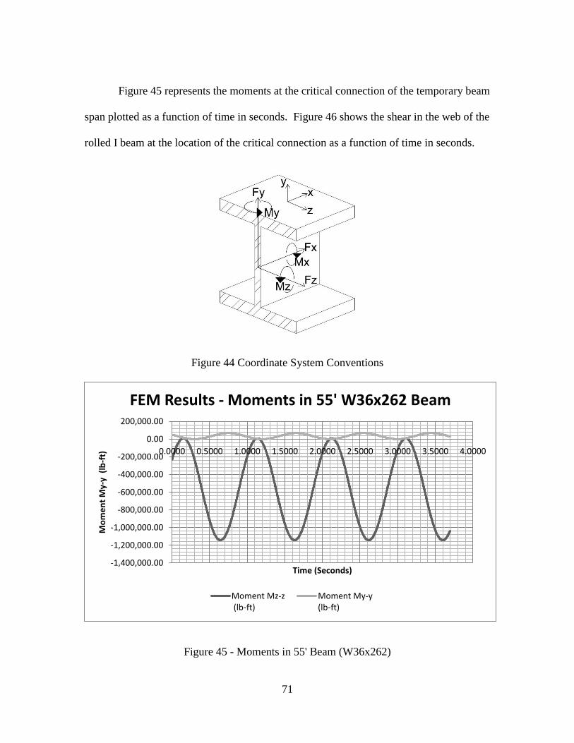
71

Figure 45 represents the moments at the critical connection of the temporary beam

span plotted as a function of time in seconds. Figure 46 shows the shear in the web of the

rolled I beam at the location of the critical connection as a function of time in seconds.

Figure 44 Coordinate System Conventions

Figure 45 - Moments in 55' Beam (W36x262)

-1,400,000.00

-1,200,000.00

-1,000,000.00

-800,000.00

-600,000.00

-400,000.00

-200,000.00

0.00

200,000.00

0.0000 0.5000 1.0000 1.5000 2.0000 2.5000 3.0000 3.5000 4.0000

Mo

me

nt

My-

y (

lb-f

t)

Time (Seconds)

FEM Results - Moments in 55' W36x262 Beam

Moment Mz-z (lb-ft)

Moment My-y(lb-ft)

72

Figure 46 - Shear in 55' Beam (W36x262)

In addition to the forces acting on the beam along its primary axis there will also

be significant stresses on the critical connection induced in the out of plane direction due

to differential deflection of the beams. The centrifugal and wind forces explained in

previous sections will induce an uneven load distribution on each of the W36x262 beams

that could lead to relatively significant differences in their maximum defections at the

location of the critical connection. Figure 47 shows how this deflection causes moment

forces and out of plane stresses in the temporary span.

-30000.00

-20000.00

-10000.00

0.00

10000.00

20000.00

30000.00

40000.00

50000.00

60000.00

70000.00

0.0000 0.5000 1.0000 1.5000 2.0000 2.5000 3.0000 3.5000 4.0000

She

ar (

lb)

Time (Seconds)

FEM Results - Shear in 55' W36x262 Beam

Shear Vy (lb)

73

Figure 47 - Differential Deflection of W36x262

Table 5 – Differential Deflections

Diaphragm

Time

Seconds

Differential

Deflection (Δ)

Abaqus

Amplification

Factor (Δ)

0.0000 -0.00447528 0.213

0.0014 -0.00439767 0.209

0.0028 -0.00432055 0.206

0.0043 -0.00424395 0.202

0.0057 -0.00416785 0.198

0.0071 -0.00409228 0.195

The out of plane forces induced by differential deflection are transferred to the

beam through the diaphragm and stiffener. An inspection of Figure 47 shows that a

tensile stress concentration is likely to be highest at the lowest point of the welded

stiffener to web connection in Beam 2. This will increase the maximum principle

stresses and reduce the fatigue life of the connection in a way that is not directly

referenced in the AREMA design manual. In order to model the complex geometry and

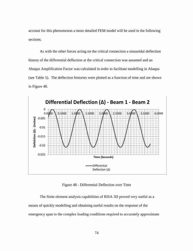
74

account for this phenomenon a more detailed FEM model will be used in the following

sections.

As with the other forces acting on the critical connection a sinusoidal deflection

history of the differential deflection at the critical connection was assumed and an

Abaqus Amplification Factor was calculated in order to facilitate modelling in Abaqus

(see Table 5). The deflection histories were plotted as a function of time and are shown

in Figure 48.

Figure 48 - Differential Deflection over Time

The finite element analysis capabilities of RISA 3D proved very useful as a

means of quickly modelling and obtaining useful results on the response of the

emergency span to the complex loading conditions required to accurately approximate

-0.025

-0.02

-0.015

-0.01

-0.005

0

0.0000 0.5000 1.0000 1.5000 2.0000 2.5000 3.0000 3.5000 4.0000

De

felc

tio

n (Δ

) -

(In

che

s)

Time (Seconds)

Differential Deflection (Δ) - Beam 1 - Beam 2

Differential Deflection (Δ)

75

real world load cases. The moving load feature proved especially well-suited to

analyzing the structure in a useful way on a macro level. However, in order to obtain a

more detailed understanding of the local response of the critical connection to the loads it

will be subjected to it was necessary to constructed a more detailed finite element model

and apply the loads obtained from the macro analysis.

76

Chapter 5

Modelling of Critical Connection Using Abaqus CAE

Using the values calculated from the macro analysis a three dimensional

representation of the critical connection was modelled using Abaqus CAE. The

combination of forces and displacements obtained from the methods outlined in the

above sections was applied to this model in order to ascertain the stress data that was

needed for a comprehensive fatigue analysis. Two stress states are required for a

comprehensive analysis of the fatigue life of the critical connection; ΔSre – the stress

range at the critical location due to applied loads and σres – the residual stress at the

critical location due to arc welding. These stresses in conjunction with the geometry of

the connection and assumed defect were then used to determine appropriate stress

intensity factors utilizing a finite element methodology for the applied loads and a weight

function for the residual stresses. This information was in turn used in a linear elastic

fracture mechanics analysis outlined later in this research in order to determine an

effective fatigue life.

5.1 Stresses Due to Applied Loads

The critical connection was modelled as a thin strip of the W36x262 beam with

the stiffener and diaphragm modelled in their entirety. The beam was subjected to the

forces calculated from the RISA 3D analysis applied to the cut face of the beam. The

moment applied to the section was modelled as a linearly variable distributive load

77

utilizing a user defined formula to achieve appropriate distribution of stresses. The

Abaqus amplitude factors outlined in Table 4 were used in the definition of the amplitude

of the load over time in order to assure a sinusoidal load history on the connection. The

diaphragm was fixed at one end and a deflection in the Y direction was induced in the

beam using a similar methodology (amplitude factors for sinusoidal history) as the loads

in order to model the effects of differential deflection over time. The loads were applied

in a step module in Abaqus with the incrimination parameters set up to emulate the time

for one complete cycle on the structure.

Figure 49 shows a contour plot of the Mises stress history of the connection over

a period of time. The region of concern in terms of the fatigue life of the critical

connection is the area at the base of the weld. It is this area that experiences the greatest

magnitude of tensile stress along the length of the weld. When considering only in plane

forces it is obvious that the extreme fiber of the beam will experience a greater magnitude

of tensile stress than the bottom of the weld connection but it is assumed that there is

much less likelihood of a defect capable of causing crack propagation being present in the

un-welded portion of the member. This coupled with the fact that out of plane stresses

are introduced by the stiffener to web connection made the area at the base of the weld a

primary concern.

78

Figure 49 - Stress Distribution at Critical Connection

The connection was modelled using 3D stress quadratic tetrahedral elements (C3D10

shown in Figure 50) with a refined mesh at the base of the weld (see Figure 49).

79

Figure 50 - C3D10 Element

Figure 51 - Principle Stresses near the Weld Toe over Time

Figure 51 shows the principle stresses near the weld toes over time and gives a

good indication of the effect out of plane stresses have on the magnitude of the stress

range. The measured stress range at the extreme fiber of the welded connection in the

FEM analysis is more than triple the allowable stress range for the fatigue category C’ in

80

the AREMA manual and is also more than double the anticipated stress range obtained

using the Cooper E loading with a strictly in plane analysis. However, inspection of the

data showed that the stress range evens out fairly quickly to more moderate levels the

further away from the extreme bottom of the weld toe the stresses are examined. Since

the region with the highest stress range is also the region most likely to develop fatigue

cracks these results alone can validate the need for this research as a tool for future use of

the emergency span.

5.2 Residual Stresses Induced by Weld

It has been extensively proven as shown in the literature [15] [16] that residual

stresses introduced by arc welding processes have a direct effect on the fatigue life of a

structural member. The use of finite element simulations to predict residual stresses in as

welded members is the subject of active study and has largely gained the acceptance of

the engineering community as a reasonably accurate prediction tool [18]. A sequentially

coupled finite element analysis was undertaken on the fillet weld of the stiffener to web

connection of the critical connection in order to ascertain the appropriate stresses (and

stress intensity factors using a weight function as outlined in later sections) associated

with the process. The following assumptions were made as to the type and process of the

weld procedure;

Shield Metal Arc Welding (SMAW)

5/16” Weld bead – Single Pass

Direct Current

81

All field welded connections

The SMAW process is the most commonly used type of field weld in the railway

industry and is assumed to be the welding process of choice for the type of rapid

construction needs associated with the emergency span erection. In the SMAW process

an electric current from a welding power supply is used to form a current between the

base material and a consumable electrode. The electric current, or arc, between the base

material and the electrode creates the extremely high temperatures (up to 6500°F at the

tip) needed to fuse the connection. The electrode is coated in flux which forms protective

gasses and slag in order to protect the weld zone from atmospheric contamination. The

high heat induced by the weld arc causes the base material to deform in a plastic manner

in the heat affected zone by introducing large stresses and strains as well as causing

thermal expansion. After the weld cools the member doesn’t completely return to its

original shape causing distortion induced stress fields. Residual stress fields in tension

can have a significant negative effect on the fatigue life of welded connections while

compressive residual stress can have a positive impact [19]. In order to facilitate the

efficient modelling and to keep model complexity reasonable a sub-section of the critical

connection was chosen for modelling as a separate analysis. Figure 52 shows the section

of model that was considered for this welding analysis. In order to best understand the

overall FEM processes and procedures an overview of heat transfer and residual stress

fundamentals as they relate to this research analysis are briefly covered in the next two

sections.

82

Figure 52 - Section of Connection Modelled for Weld Analysis

5.2.1 Thermal Heat Effects Caused by Welding

Heat flow as passed from the arc or torch to the base material is of principle

concern in the study of a thermal FEM analysis. In arc welding the total heat output is a

product of the current and the voltage when considering a direct current. This can be

expressed as [15];

𝑄 = 𝑉𝐼𝜂ℎ𝑒𝑎𝑡 (Equation 20)

Where

V = Voltage

83

I = Current

𝜂ℎ𝑒𝑎𝑡 = Process dependent heat efficiency

For the Purposes of FEM modelling the heat generated can be expressed as:

𝑄 = 𝑄𝑆 + 𝑄𝑉 + 𝑄𝑓 (Equation 21)

Where

QS = Surface heat

QV = Volume heat

Qf = Filler heat generated by the addition of the bead material

For the FEM analysis to output a usable heat history the heat fields are needed as

a function of time and space. In order to describe the temperature fields in an isotropic

continuum element with temperature dependent material properties over time the

following equation is utilized in the FEM formulation;

𝜕𝑇

𝜕𝑡= 𝛼 (

𝜕2𝑇

𝜕𝑥2+

𝜕2𝑇

𝜕𝑦2+

𝜕2𝑇

𝜕𝑧2) +

1

𝑐𝜌

𝜕𝑄𝑉

𝜕𝑡

(Equation 22)

Where,

𝜕𝑇

𝜕𝑡 = is the rate of change in temperature at a point over time

84

T = T(x,y,z,t) is temperature as a function of space and time

𝜌 = density

𝛼 = 𝑘

𝑐𝜌 is the thermal diffusivity

K = Thermal conductivity

C = specific heat capacity

When a usable heat transfer analysis over time is compiled with the finite element

method the results are written to and input file that can be used in a subsequent stress

analysis.

5.2.2 Residual Stresses

Residual stresses are primarily caused by the variation of temperature across a

region or volume whose magnitude can be calculated using the above equations. These

stresses, termed thermal stresses, will dissipate as the temperature variance evens out. In

the case of welded steel connections the heat variance becomes high enough for plastic

deformation to occur. Due to thermal expansion in the heated region an elastic

compressive zone is formed with the surrounding colder material. When the plastically

compressed region cools it gives way to a tension stress field. It is these stress fields that

will have a direct negative effect on the fatigue life of the temporary span.

85

5.2.3 FEM Procedure

The FEM analysis as performed using Abaqus software was approached using the

sequentially coupled Thermal-Stress analysis method discussed above. Weld beads were

modelled by partitioning the three dimensional region of the part meant to represent the

weld material. The weld arc was simulated by applying a user defined temperature of

2740°F (which is the melting temperature of A572 Gr 50 Carbon Steel) at the boundary

between the partitioned beads and the interaction surfaces of the model. The beads were

activated in the model sequentially over time by applying an Abaqus “model change” in a

separate step for that bead. The beads only interact with beads from previous steps that

have been activated in an Abaqus model change but beads that have yet to be activated

are still allowed to deform with the model in order to avoid convergence issues. These

beads had no effect on the stiffness of the system since they were considered to be near

their melting point and therefore very ductile. The arc/torch application was analyzed

through transient heat transfer steps and then a cool down step was introduced that

deactivated the boundary conditions associated with the heating step. The values for the

heat transfer were then fed into the static stress analysis as a loading history. The

coupled analysis relies heavily on temperature dependent material properties and

complex boundary conditions that can be researched extensively by an examination of the

literature [20] [21] [22] [23]. Figure 53 shows a schematic of the modelling process and

analysis steps.

86

5.2.4 FEM Results

The results from the FEM analysis of the web to stringer welding process were

examined and compared to a range of studies that presented empirical data on welded

connection residual stresses as well as some FEM based analysis to ensure that a

reasonable result was obtained [14] [15] [18] [25] [26] [27]. One of the driving goals of

Define Geometry of Base and Weld

Model T-Section and weld

Partition weld to create individual

beads for time dependent

application

Define global boundary conditions

Define Material Properties

Mesh Part

Conduct Stress Analysis

Preform a static stress

analysis

Use heat transfer as a

loading history

Mechanical material

property dependent

Post-Processing

Transverse residual

stresses

Longitudinal residual

stresses

Heat transfer history

Conduct Heat Transfer Analysis

Define weld path

Create a step for each bead to be

removed then reapplied to model

with thermal transfer conditions

activated

Thermal material property

dependent

Figure 53 - Schematic of FEM Modelling Process for

Welded Connection

87

the FEM analysis was to obtain the transverse residual stresses induced at the weld toe of

the connection as these stresses will play a significant role in the estimation of fatigue life

as discussed in later sections of this paper. Results were plotted both with regard to time

and distance (in inches) away from the weld toe using the conventions outlined in Figure

54.

Figure 54 - Plot Convention for

Distance Results

Figure 55 - Stress Contour Plot of the Heat

Affected Zone (HAZ)

Figure 56 - Temperature as a function of time for sample elements along the X-axis

88

Results for longitudinal (Figure 58) and transverse (Figure 60) residual stresses

show good agreement with neutron defraction measurements and finite element method

predictions as presented in the literature for similar type weldments [14] [27]. The

transverse residual effects are considered to control for the purposes of fatigue estimation

for the geometry of the critical connection as defects are most likely to coincide with the

edge of the weld toe and propagate normal to the transverse stress field. Figure 56 shows

the temperature in the connection at several elements over time. The analysis considered

that one side of the stiffener would be welded before the other and, as a result, even

though the analysis considers a single weld pass the area around the weld would be

heated twice as the arc moved across the opposite side. The results in the time period 400

– 700 in Figure 56 clearly demonstrate the effect this assumption has on the analysis.

89

Figure 57 - Misses Stresses at Weld

90

Figure 58 - Longitudinal Residual Stress along X-axis

The behavior of the stress distribution showed a good agreement with the

principles of residual stress behavior as outlined earlier in this section. Figure 58 shows

the tension zone near the weld toe giving way to a compressive residual stress field

further along the x-axis. The transverse residual stress plot over time shown in Figure 59

also indicates good agreement with the anticipated behavior of the weld by showing that

peak compressive stresses as the weld arc passes over the element give way to a reversal

into a tensile stress field as the cooling step takes effect.

The size of the sub-model and the boundary conditions that were used in the FEM

analysis were carefully chosen in order to balance accurate results with the complexity

and time constraints associated with running the analysis. The stiffness of the system has

a direct effect on the concentration of residual stress as thermal expansion generates

91

compressive stresses in the surrounding material. If a system is too stiff it will show

unrealistically high residual stresses. The cross section of the model was carefully chosen

to ensure that these forces had enough volume to dissipate heat energy at an acceptable

level, especially in the transverse direction (see Figure 55). The model is likely stiffer in

the longitudinal direction than real world conditions which may lead to somewhat higher

longitudinal stresses than would be experienced in the field. However, the predicted

results still fall within a reasonably accurate range of expected results.

Figure 59 – Transverse Residual Stress near Weld Toe over Time

92

Figure 60 - Transverse Residual Stress along X-axis

93

Chapter 6

Fatigue Life Assessment Utilizing LEFM

Linear elastic fracture mechanics (LEFM) is the study of crack propagation within

solids subjected to stresses that produce a linear elastic response. It is an extremely

important tool for determining the fatigue life of details with pre-existing defects. In

order to gain a better understanding of the basic concepts associated with the

implementation of LEFM and how it was utilized in the context of this research study a

general overview of LEFM is presented.

6.1 Overview of Linear Elastic Fracture Mechanics

LEFM is an analytical approach to crack propagation that relates the stress field

magnitude and distribution near a crack tip to the applied stresses, size / shape /

orientation of the crack, and material properties. The fundamental principle of LEFM is

that the stress field ahead of a crack tip can be characterized by a stress intensity factor

(SIF). In order to analyze the stresses at the crack tip in an elastic solid it is common

practice in classic LEFM to define the relative movements of two crack surfaces as

modes. Theses modes represent the local displacements in an infinitely small element

containing a crack singularity and are shown in Figure 61.

94

Figure 61 - Modes of Crack Surface Displacement

Mode I is characterized by a tensile induced opening of the crack surfaces relative

to one another and is usually the driving mode in terms of crack behavior for most

engineering applications [19]. Mode II is the result of in plane shearing of the surfaces

and Mode III is characterized by out-of-plane shearing effects. The stress intensity factor

for each of the three failure modes can be expressed as a limit with r approaching zero

and stress as a function of r and θ as shown in (Equation 23), (Equation 24) and

(Equation 25).

𝐾𝐼 = lim𝑟→0

√2𝜋𝑟 𝜎𝑦𝑦(𝑟, 𝜃) (Equation 23)

𝐾𝐼𝐼 = lim𝑟→0

√2𝜋𝑟 𝜎𝑦𝑥(𝑟, 𝜃) (Equation 24)

95

𝐾𝐼𝐼𝐼 = lim𝑟→0

√2𝜋𝑟 𝜎𝑦𝑧(𝑟, 𝜃) (Equation 25)

Where r and θ are shown in Figure 62 relative to the coordinate system and stress

components;

Figure 62 - Stress Components and Global Coordinates ahead of a Crack

The range in stress intensity factor at a defect (ΔKI, II, III) is one of the driving

parameters affecting the propagation of cracks and can be expressed by (Equation 26).

∆𝐾𝐼,𝐼𝐼,𝐼𝐼𝐼 = 𝐾𝐼,𝐼𝐼,𝐼𝐼𝐼 𝑚𝑎𝑥 − 𝐾𝐼,𝐼𝐼,𝐼𝐼𝐼 𝑚𝑖𝑛 (Equation 26)

Where,

96

𝐾𝐼,𝐼𝐼,𝐼𝐼𝐼 𝑚𝑎𝑥 = The maximum stress intensity factor under cyclic loading for modes I, II,

and III

𝐾𝐼,𝐼𝐼,𝐼𝐼𝐼 𝑚𝑖𝑛 = The minimum stress intensity factor under cyclic loading for modes I, II,

and III

A method for relating the change in SIF to crack propagation rate and the number

of cycles to failure was developed by P. C. Paris in the early 1960s and is the most widely

used method for determining fatigue life using LEFM [28]. The equation proposed by

Paris is known as the Paris-Ergodan Power Law and can be expressed as;

𝑑𝑎

𝑑𝑁= 𝐶∆𝐾𝑚

(Equation 27)

Where,

𝑎 = Crack length

𝑁 = Total number of constant amplitude stress range cycles

𝑚 = Material constant derived from regression analysis and taken as 𝑚 = 3 for structural

steel

𝐶 = Coefficient of crack growth

Integration of (Equation 27) yields;

97

𝑁 =1

𝐶∫

𝑑𝑎

∆𝐾𝑚

𝑎𝑓

𝑎𝑖

(Equation 28)

Where,

ai = Initial crack length

af = Final crack length

Crack growth can be divided into three growth regions based on stress intensity

parameters (see Figure 63). It is assumed that there is a region where the change in SIF

(ΔK) will not be of sufficient magnitude to propagate a crack within the context of

LEFM. This region is referred to as Region I. Region II is the region that is of concern

when utilizing LEFM and constitutes the region in which cracks are assumed to

propagate at a constant rate when subjected to constant amplitude cyclic loading. The

value separating these two regions is known as the threshold value (ΔKth). Any applied

SIF range below this threshold will not cause appreciable crack growth behavior. Region

III deals with rapid fracture of the crack material and occurs when ΔK exceeds the

fracture toughness range (ΔKc) of the material.

This study covers only the behavior of the material in Region II with Region I

stresses considered to have infinite fatigue life and Region III stresses considered to have

experienced structural failure.

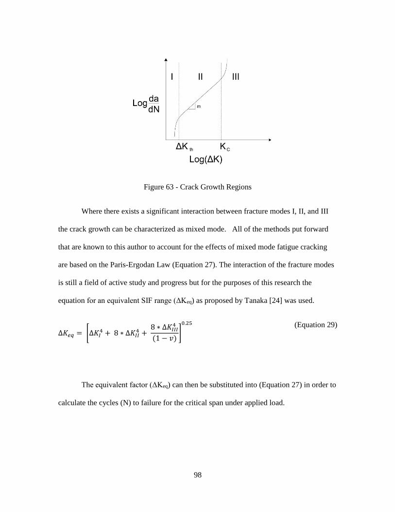
98

Figure 63 - Crack Growth Regions

Where there exists a significant interaction between fracture modes I, II, and III

the crack growth can be characterized as mixed mode. All of the methods put forward

that are known to this author to account for the effects of mixed mode fatigue cracking

are based on the Paris-Ergodan Law (Equation 27). The interaction of the fracture modes

is still a field of active study and progress but for the purposes of this research the

equation for an equivalent SIF range (ΔKeq) as proposed by Tanaka [24] was used.

∆𝐾𝑒𝑞 = [∆𝐾𝐼4 + 8 ∗ ∆𝐾𝐼𝐼

4 + 8 ∗ ∆𝐾𝐼𝐼𝐼

4

(1 − 𝑣)]

0.25

(Equation 29)

The equivalent factor (ΔKeq) can then be substituted into (Equation 27) in order to

calculate the cycles (N) to failure for the critical span under applied load.

99

6.2 Defects in the Critical Connection

Defects that arise as a consequence of the welding procedure have a significant

effect on the fatigue life of any welded structure. Some of the most common defects

associated with welded connections are cold laps, weld toe cracks and root defects. Of

these defects it has been shown in various literature [12] [13] that as many as 80% of

initial welding defects are cold laps. Cold laps form when the toe of a weld remains cold

enough that it doesn’t fuse to the base metal and the weld simply overlaps the base

material. This leaves no continuity between the two surfaces and allows for a

concentration of stresses to build up at the tip of the overlap (see Figure 64). Cracks at

the toe or root of the weld are another common type of defect and are mainly caused by

transverse shrinkage due to improper pre-heating, an influx of hydrogen in the weld pool

by way of moisture in the HAZ and a sufficient amount of transverse residual stress. For

this research it is assumed that some form of weld defect i.e. crack is present at the

critical connection prior to the emergency span being released into service. For the

purposes of fatigue life calculation this assumption should prove to be conservative.

However, it should be noted that the majority of the fatigue life in as welded connections

is consumed by the propagation phase [14]. The assumption of an initial crack being

present at the weld toe is particularly appropriate when considering that the critical

connection is intended to be welded in the field in an emergency situation. The weld site

will not be in a controlled environment and will be open to the elements, thus increasing

the possibility of moisture related cracking issues. The skill level and experience of the

welder coupled with a less strenuous inspection procedure are other variables that will

100

affect the quality of the weld in terms of possible defect. This research has assumed an

initial defect in the weld toe with a length of approximately 0.05 inches (1 mm) and a

depth of 0.03 inches (0.76 mm). These estimates are consistent with studies of defect

measurements in the literature and should prove to be conservative in terms of size and

placement [12] [13].

Figure 64 - Weld Defects

In order to determine the fatigue life in the critical connection the stress intensity

factors at the tip of the assumed crack were calculated for both the applied and residual

stresses as outlined in the next sections.

6.3 Stress Intensity Factor at the Critical Connection Due to Applied Loads

In order to calculate the SIF due to applied load at the critical connection a global

model was used to drive the stresses in a sub-model with an assumed defect of

dimensions 0.05 inches long and 0.03 inches in depth (see Figure 65). The crack was

modelled near the toe of the weld with the weld to base material transition given a 0.01

inch fillet to help avoid singularity issues in the stress formulation. The results of the

analysis show excellent agreement with the predicted behavior of stress and strain fields

101

corresponding to the shape and size predicted in the literature [19] [14] [15]. The FEM

formulation for the SIFs was carried out in FRANC3D utilizing the Interaction Integral

and Displacement Correlation Methods, both of which showed good agreement with one

another.

Figure 65 - Refined Mesh at Point of Crack

Figure 66 - Plastic Zone at Tip of Crack

(Surface)

Figure 66 shows the plastic zone that forms at the tip of the crack at the surface of

the model and Figure 67 shows the plastic zone at the crack tip for the through material

thickness defect. The crack was modelled as a semi-elliptical toe/root crack (see Figure

68) cutting perpendicular to the surface of the web as opposed to a cold lap that would

have had an initial alignment parallel to the surface. The root crack is expected to have a

more rapid fatigue growth rate and as such provided for more conservative results. In

order to predict the crack growth rate on the surface of the web as well as in the through

plate direction it is necessary to solve the SIFs for the entire length of the defect. Figure

69 and

Table 6 show the values for the SIF along the length of the crack.

102

Figure 67 - Plastic Zone at Tip of

Crack (Through Crack)

Figure 68 - Cross Section of Defect

Figure 69 - Plot of Stress Intensity Factors for the Assumed Defect

103

Table 6 - Stress Intensity Factors and Coordinates

N Coordinates KI KII KIII X Y Z

0.009 12251.11 475.2239 -543.044 -2.26 -15.2001 -0.4189

0.0268 11947.41 194.3362 -720.966 -2.26 -15.2004 -0.4166

0.0444 11713.5 -24.8045 -853.479 -2.26 -15.2009 -0.4144

0.0618 11561.72 -249.667 -949.634 -2.26 -15.2017 -0.4124

0.0793 11465 -470.987 -1010.42 -2.26 -15.2027 -0.4104

0.0968 11396.07 -681.811 -1044.32 -2.26 -15.2039 -0.4085

0.1144 11345.44 -881.45 -1060.52 -2.26 -15.2052 -0.4067

0.1321 11325.94 -1062.91 -1055.91 -2.26 -15.2067 -0.405

0.1498 11318.07 -1224.16 -1035.07 -2.26 -15.2084 -0.4034

0.1676 11323.64 -1368.23 -1004.39 -2.26 -15.2101 -0.402

0.1852 11335.6 -1503.35 -965.084 -2.26 -15.2119 -0.4006

0.2026 11360.21 -1626.31 -920.413 -2.26 -15.2137 -0.3994

0.2203 11412.59 -1733.34 -875.54 -2.26 -15.2157 -0.3982

0.2384 11457.95 -1831.33 -836.26 -2.26 -15.2177 -0.3971

0.2565 11483.79 -1921.5 -791.977 -2.26 -15.2198 -0.3961

0.2746 11514.29 -1998.91 -744.236 -2.26 -15.2219 -0.3952

0.2926 11545.24 -2063.92 -692.608 -2.26 -15.224 -0.3944

0.3107 11573.7 -2124.88 -639.592 -2.26 -15.2262 -0.3936

0.3287 11589.05 -2178.88 -587.442 -2.26 -15.2284 -0.3929

0.3468 11603.12 -2236.66 -529.857 -2.26 -15.2306 -0.3923

0.3649 11623.23 -2290.25 -470.243 -2.26 -15.2329 -0.3918

0.3829 11633.07 -2335.55 -412.252 -2.26 -15.2351 -0.3914

0.401 11654 -2372.62 -356.274 -2.26 -15.2374 -0.391

0.4191 11662.35 -2407.54 -301.246 -2.26 -15.2397 -0.3907

0.4371 11673.23 -2431.59 -244.212 -2.26 -15.242 -0.3904

0.4551 11674.88 -2448.87 -187.038 -2.26 -15.2443 -0.3902

0.4731 11670.39 -2466.05 -132.452 -2.26 -15.2466 -0.3901

0.491 11662.46 -2475.65 -78.6377 -2.26 -15.2489 -0.39

0.509 11661.6 -2477.65 -10.0873 -2.26 -15.2511 -0.39

0.527 11678.03 -2477.82 40.2342 -2.26 -15.2534 -0.3901

0.5451 11679.34 -2465.76 93.4779 -2.26 -15.2557 -0.3902

0.5631 11662.22 -2450.88 146.3889 -2.26 -15.258 -0.3904

0.5812 11640.82 -2423.32 199.5429 -2.26 -15.2603 -0.3907

0.5993 11621.3 -2392.22 258.3933 -2.26 -15.2626 -0.391

0.6174 11608.25 -2359.35 318.4164 -2.26 -15.2649 -0.3914

0.6355 11592.64 -2324.71 378.7105 -2.26 -15.2672 -0.3918

0.6535 11563.81 -2287.34 441.38 -2.26 -15.2694 -0.3924

0.6716 11552.97 -2237.72 503.6691 -2.26 -15.2716 -0.393

0.6896 11530.17 -2180.07 563.1044 -2.26 -15.2738 -0.3936

0.7076 11500.83 -2116.56 619.931 -2.26 -15.276 -0.3944

0.7257 11483.68 -2048.95 675.0282 -2.26 -15.2781 -0.3952

0.7437 11466.77 -1970.61 728.47 -2.26 -15.2802 -0.3961

0.7617 11448.76 -1881.56 775.9277 -2.26 -15.2823 -0.3971

0.7798 11412.44 -1775.97 814.4756 -2.26 -15.2843 -0.3982

0.7975 11361.73 -1660.31 860.7024 -2.26 -15.2863 -0.3994

0.8149 11330.91 -1526.59 908.3927 -2.26 -15.2881 -0.4006

0.8326 11325.48 -1388.5 947.3525 -2.26 -15.2899 -0.402

0.8504 11327.23 -1238.87 977.2256 -2.26 -15.2917 -0.4034

0.8681 11326.85 -1076.42 995.8143 -2.26 -15.2933 -0.405

0.8858 11334.3 -896.945 1002.612 -2.26 -15.2948 -0.4067

0.9035 11368.93 -705.81 989.4372 -2.26 -15.2961 -0.4085

0.921 11436.21 -503.286 957.9431 -2.26 -15.2973 -0.4104

0.9384 11533.29 -291.945 900.0378 -2.26 -15.2983 -0.4124

0.9558 11680.56 -73.6223 807.0489 -2.26 -15.2991 -0.4144

0.9733 11910.48 138.7492 679.6187 -2.26 -15.2996 -0.4166

0.991 12213.54 405.697 507.1156 -2.26 -15.2999 -0.4189

104

6.4 Stress Intensity Factor at the Critical Connection Due to Residual Stresses

The SIF due to residual stresses (Kres) was calculated using a weight function and

incorporated into the LEFM fatigue analysis by way of the mean stress method. This

approach makes the determination that transverse residual stresses acting normal to the

assumed defect will be the predominate form of residual stress driving crack growth.

(Equation 30) was used to calculate the stress intensity factor due to residual stress (Kres)

𝐾𝑟𝑒𝑠 = 𝜎𝑟𝑒𝑠√𝜋𝑎

𝑄∗ ℎ(𝑎, 𝑡)

(Equation 30)

Where,

𝜎𝑟𝑒𝑠 = Residual stress affecting crack propagation and taken as

𝑎 = Depth of assumed crack into base material

𝑡 = Thickness of the steel web

ℎ(𝑎, 𝑡) = Weight function

𝑄 = Φ02 With the value taken from Barson and Rolfe [19] Table 2.13 page 47

For a more detailed explanation of the weight function assumed for this analysis

as well as a list of weight functions used for various geometries please examine the work

of Barsom and Rolfe [19] and Fett et al [29] [30] [31].

105

The stress intensity factor due to residual stresses was then incorporated into the

LEFM analysis by way of the mean stress method using the following equation for R

greater than or equal to 0.

𝑑𝑎

𝑑𝑁=

𝐶(∆𝐾)3

√1 − 𝑅

(Equation 31)

Where,

R = The load ratio. Taken as 𝐾𝑒𝑞 𝑚𝑖𝑛+ 𝐾𝑟𝑒𝑠

𝐾𝑒𝑞 𝑚𝑎𝑥 +𝐾𝑟𝑒𝑠

6.5 Fracture Toughness, Coefficient of Crack Growth and Critical Crack Length

Before the Paris Ergodan Miner Law could be utilized to solve for fatigue life at

the critical connection the Paris Law parameters (C and m) and final crack length (af)

were required. The final crack length (af) was considered to occur at a point where the

crack transitioned from stable to unstable growth or in other words moved from region II

to region III growth characteristics (see Figure 63). The length of crack required for this

to occur is known as the critical crack length and is a function of the fracture toughness

and the design stress present in the connection [19]. For the purposes of this research it is

considered that;

𝑎𝑓 = 𝑎𝑐 (Equation 32)

Where,

106

𝑎𝑐 = The critical crack length

The critical crack length for the critical connection can be found using the following

equation [19].

𝑎𝑐 = 1

𝜋(

𝐾𝐼𝐶

𝜎𝑚𝑎𝑥)2

(Equation 33)

Where,

𝜎𝑚𝑎𝑥 = The maximum stress present at the critical location

𝐾𝐼𝐶 = The critical fracture toughness of the material

Note that (Equation 33) is valid for a crack that propagates along the face of the

steel surface. The crack assumed at the critical connection will almost certainly spread in

this manner; however, the crack will likely propagate into the thickness of the material as

well. For the purposes of this research this author has elected to consider the thickness of

the W36x262 web (0.84”) to be the critical crack length for a defect that propagates

normal to the plate surface. This approach is consistent with the best practices for fatigue

control within the railway industry [1] [2].

The value of KIC is typically determined by a testing method that accounts for the

toughness directly. However it is possible in many cases to estimate the value of KIC

using energy absorption data from a test such as the Charpy V-notch test (CVN) when no

other means are available [33]. The Chary V-notch test is a standardized high strain-rate

107

test that yields information on a material’s notch toughness by measuring the amount of

energy absorbed by a material during brittle fracture. It is usually given with results for

three separate impacts. Table 7 shows the Charpy V-notch data obtained for the

W36x262 A572 Gr. 50 steel beams used for the emergency span.

Table 7 - Charpy V-notch Data for Emergency Span

Rolfe and Barsom et al proposed that the following equation can be used to

estimate the value of KIC using Chary energy data [34].

(𝐾𝐼𝐶

𝑓𝑦)

2

= 5

𝑓𝑦 (𝐶𝑉𝑁 −

𝑓𝑦

20)

(Equation 34)

Where,

𝑓𝑦 = The yield strength of the steel material

𝐶𝑉𝑁 = Charpy V-notch energy absorption

Conservatively using a value of 𝑓𝑦 = 50 ksi (62 ksi would also be acceptable

based on Table 7) and utilizing (Equation 34) gives a value of for 𝐾𝐼𝐶 of 144.5 ksi√𝑖𝑛.

Yield

Strength

Tensile

StrengthELONG Temp

KSI KSI % F

Mpa Mpa % C

62 76 28.1 10 F 86 90 94

427 524 28 -12 C 117 127 1210.82

Mechanical Properties Chemical Properties

Yield Tensile

Ratio CI

0.002 0.01 0.41 0.19 6.5

V

0.04

Cb CE Sn PcmMo

0.07 1.25 0.016 0.018 0.26 0.33 0.27 0.4 0.04

P S Si Cu Ni Cr

Imapact Energy

FT-LBS

JOULES

C Mn

108

Plugging the value for 𝐾𝐼𝐶 and the stress values for the critical connection shown

in Figure 51 into (Equation 33) yields a value for 𝑎𝑐 and 𝑎𝑓 of 3.77 inches which is

consistent with experimental data found in Barsom and Rolfe [19].

Another variable that needed to be addressed before a fatigue analysis became

possible was the establishment of a quantifiable connection between steel microstructure

and crack growth. It has been shown in the literature [19] [34] that the fatigue crack

growth behavior in steels can be subdivided into three main microstructural groups;

ferrite-pearlite, martensitic and austentic. The crack growth behavior in each of these

steel microstructure groups can be estimated to a reasonable degree of accuracy

regardless of any variation in tensile strength and chemical composition [19]. The A572

Gr. 50 structural steel considered for the construction of the emergency span falls into the

ferrite-pearlite category along with most structural steels.

Like all steels, ferrite-pearlite steels are created by adding a small amount of

carbon to iron in order to produce a material with superior mechanical properties. Since

the carbon atom’s atomic diameter is less than the interstices of the iron crystal lattice the

carbon will dissolve into the iron lattice and cause a distortion of the crystalline structure

of the iron atoms when heated during the fabrication process (see Figure 70). Ferrite-

pearlite steel is then produced by allowing the heated steel to cool at a very slow rate

during the manufacturing process. This allows ferrite-pearlite steel to exhibit a much

finer microstructure than steels that are cooled more rapidly. It is this microstructural

density that will have a direct effect on crack propagation as it pertains to this research.

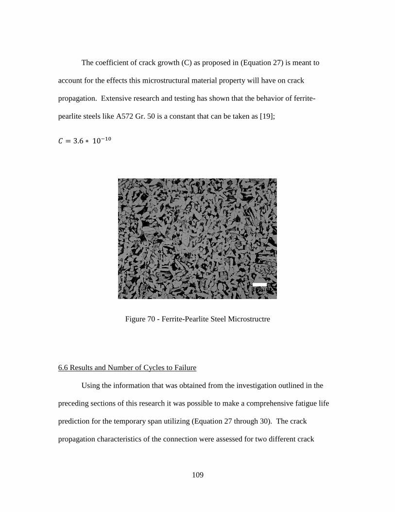
109

The coefficient of crack growth (C) as proposed in (Equation 27) is meant to

account for the effects this microstructural material property will have on crack

propagation. Extensive research and testing has shown that the behavior of ferrite-

pearlite steels like A572 Gr. 50 is a constant that can be taken as [19];

𝐶 = 3.6 ∗ 10−10

Figure 70 - Ferrite-Pearlite Steel Microstructre

6.6 Results and Number of Cycles to Failure

Using the information that was obtained from the investigation outlined in the

preceding sections of this research it was possible to make a comprehensive fatigue life

prediction for the temporary span utilizing (Equation 27 through 30). The crack

propagation characteristics of the connection were assessed for two different crack

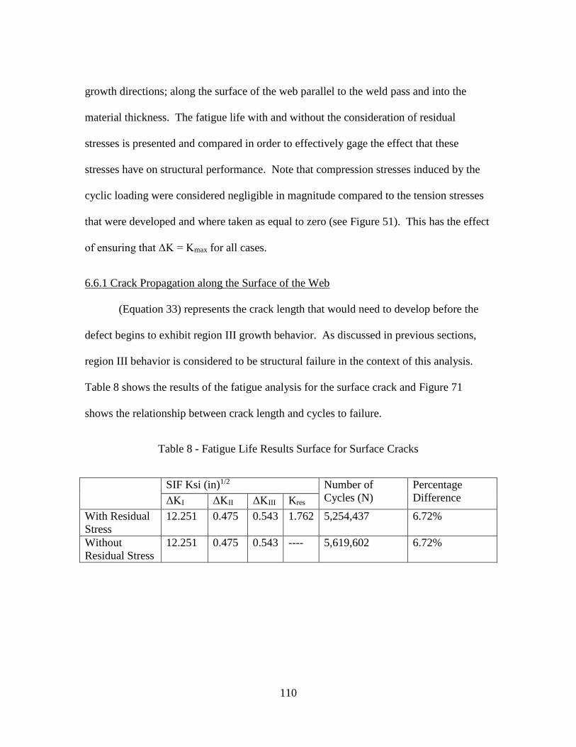
110

growth directions; along the surface of the web parallel to the weld pass and into the

material thickness. The fatigue life with and without the consideration of residual

stresses is presented and compared in order to effectively gage the effect that these

stresses have on structural performance. Note that compression stresses induced by the

cyclic loading were considered negligible in magnitude compared to the tension stresses

that were developed and where taken as equal to zero (see Figure 51). This has the effect

of ensuring that ΔK = Kmax for all cases.

6.6.1 Crack Propagation along the Surface of the Web

(Equation 33) represents the crack length that would need to develop before the

defect begins to exhibit region III growth behavior. As discussed in previous sections,

region III behavior is considered to be structural failure in the context of this analysis.

Table 8 shows the results of the fatigue analysis for the surface crack and Figure 71

shows the relationship between crack length and cycles to failure.

Table 8 - Fatigue Life Results Surface for Surface Cracks

SIF Ksi (in)1/2 Number of

Cycles (N)

Percentage

Difference ΔKI ΔKII ΔKIII Kres

With Residual

Stress

12.251 0.475 0.543 1.762 5,254,437 6.72%

Without

Residual Stress

12.251 0.475 0.543 ---- 5,619,602 6.72%

111

Figure 71 - Relationship between Crack Length and Cycles to Failure (Surface Crack)

6.6.2 Crack Propagation into Thickness of Material

Stress intensity factors taken from

Table 6 and located at the center of the half elliptical defect being analyzed were

used to determine the propagation rate of the crack through the thickness of the steel web.

The results of the analysis are listed in Table 9 and the relationship between crack length

and number of cycles to failure is shown in Figure 72.

0.00

0.50

1.00

1.50

2.00

2.50

3.00

3.50

4.00

10,000 50,000 250,000 1,250,000 6,250,000

Len

gth

of

Cra

ck (

a)

Number of Cycle (N) to Failure

Crack Propagation across Surface

N

N(res)

112

Table 9 - Fatigue Life Results for Through Thickness Crack Growth

SIF Ksi (in)1/2 Number of

Cycles (N)

Percentage

Difference ΔKI ΔKII ΔKIII Kres

With Residual

Stress

11.7 -2.448 -0.187 1.762 1,263,156 6.99%

Without

Residual Stress

11.7 -2.448 -0.187 ---- 1,354,599 6.99%

Figure 72 - Relationship between Crack Length and Cycles to Failure (Through Crack)

6.7 Discussion of Results

A number of interesting points were learned from the results obtained in this research

analysis. Some of the most important takeaways from the above results are categorized

below;

0.00

0.10

0.20

0.30

0.40

0.50

0.60

0.70

0.80

0.90

10,000 50,000 250,000 1,250,000

Len

gth

of

Cra

ck (

a)

Number of Cycles (N) to Failure

Crack Propagation into Base Material

N

N(res)

113

Through thickness propagation of defects present at the weld toe in the form of

cold laps or toe/root cracks are most likely to be the controlling design life

parameter of the temporary span.

The emergency span’s expected design life is a conservative approximation of N

= 1.263e6 cycles. This is less than the 2 million cycles required for a permanent

railway structure according to AREMA [1].

The effects of residual stresses on the effective fatigue life of the temporary span

are relatively minimal. Examination of Table 8 and Table 9 show that the average

reduction in design life when considering residual stresses are around 7% for the

temporary span.

For the purposes of fatigue calculations, AREMA Committee 15 estimated an

upper limit of rail traffic on any given rail line to be about 20 trains a day with 2

locomotives carrying 150 railcars [1]. This kind of heavy traffic utilizing 315K

railcars is not a reality on the present day railway system but it will make for a good

approximating of the absolute maximum amount of cycles that the emergency span

can be feasibly subjected to in the near future. When converting those trains to

equivalent cycles on the temporary span one can deduce from this research that the

span can be expected to perform with confidence for a minimum of 421 days. This is

more than enough time for a replacement span to be designed, fabricated and built.

It is also worth noting that the bridge engineer confronted with the challenge of

having to use the emergency span will have access to a complete loading history of

114

the structure that is to be replaced. Comparing those documents to the findings put

forth in this research paper will allow the engineer to make decisions about how long

the span can be left in place. In fact, on some parts of the railway system that carry

lighter traffic it might be feasible to use the temporary structure as a semi-permanent

replacement for the damaged bridge. This would allow for an excellent opportunity

to study the response of the emergency structure in real world conditions as a means

of comparison with the FEM findings.

Any use of the temporary structure on a class 1 railway mainline for a period of

longer than 421 days would likely require a specialized inspection procedure. The

weldments in the tension zone at the critical connection would be of primary

importance in regard to inspections.

As mentioned earlier the residual stresses induced by the welding process had a

surprisingly small effect on the fatigue life of the temporary span. While this is at

first somewhat surprising, an inspection of Figure 58 and Figure 60 should make it

clear that the orientation of the assumed crack was the primary driver in this result.

The magnitude of the predicted longitudinal residual stress is much greater than the

predicted transverse stress. Since mode I parameters are the preeminent driver of

fatigue crack growth in the context of LEFM and the assumed crack was oriented for

mode I interaction with the transverse and not longitudinal residual stresses it stands

to reason that the residual stress effects would be lower. If the crack were oriented

normal to the weld pass then the residual stresses would have a much larger role in

115

the fatigue life while the tensile stress from the applied load would play a much

smaller role.

116

Chapter 7

Summary, Conclusions and Future Work

7.1 Summary

The problem of providing a flexible solution to the challenge of service outages

on railway lines due to vehicle or other impacts to railway bridge infrastructure is

explored in this study with a particular interest on the fatigue service life of welded

connections for the proposed solution. A systematic overview of the current state of

temporary and rapid bridge construction techniques is undertaken and the strengths and

weaknesses of these solutions are discussed. A new type of temporary span is then

proposed to service the use cases that are not covered by current practices. The design,

configuration and construction methods of this proposed emergency span is then detailed

and examined using the current industry standard Copper-E design loads. In order to

save on construction time and to accommodate skewed substructure configurations the

emergency span is designed to utilize welded connections for the diaphragms and

stiffener plates. It is shown that even under Cooper-E loads this detail falls outside the

allowable stress range for the AREMA fatigue category to which it belongs, thus

validating the need for further analysis.

Once the need for further analysis into the service life of the critical welded

connection is confirmed it is proposed to use finite element analysis along with more

representative loading conditions to determine the fatigue life of the connection. In order

to facilitate the most efficient means of achieving this result the analysis is broken into

117

three phases using the methods and FEA software that makes the most sense for each

phase. Phase 1 constitutes a macro analysis of the structure using RISA 3D to determine

the location of the critical connection and the stresses induced at the location by the

prescribed loads. Phase 2 builds on the information obtained in Phase 1 to build a

detailed model of the critical connection in Abaqus CAE. Phase 3 leverages the

principles of linear elastic fracture mechanics in order to predict the fatigue life to the

connection and make recommendation in regard to its effective use.

In order to most accurately predict the structural response of the temporary

structure in Phase 1 it was decided to use loading conditions that are representative of the

actual equipment that will be used on the structure both presently or in the near future

(Ex: 435K locomotives and 315K railcars). This is in contrast to the AREMA loads that

are based on outdated steam locomotive geometry from a time when fatigue conditions

were not well understood. Once the appropriate loads were identified the temporary

structure was modelled in RISA 3D in order to take advantage of the rapid modelling and

moving load capabilities of the software. A loading history was then interpolated from

the results of the RISA analysis to be used in the subsequent phases of the study.

Once the load history of the critical connection was established the results were

fed into a more detailed model of the connection that was modelled using Abaqus CAE

for Phase 2. The Phase 2 analysis consisted of two main objectives; determine the

stresses in the connection due to applied loads and determine the residual stresses

induced by the welding process. Two separate models of the connection were utilized for

118

this purpose using 3D stress quadratic tetrahedral elements. The stresses due to applied

loads were determined by applying the combination of forces and displacements

calculated in the first phase using the loading history and the calculated amplitude factors

to ensure appropriate distribution of stresses. To determine the residual stresses due to

shield metal arc welding a sequentially coupled finite element analysis was performed on

a smaller section of the connection that was modelling using Abaqus CAE.

The final phase of this research uses linear elastic fracture mechanics to predict

the growth of a crack from a preexisting defect that was conservatively assumed to have

occurred during the welding process before the span was released into service. A sub

model of the defect was subject to the forces due to applied loads calculated in phase 2 in

order to determine the stress intensity factor. The stress intensity factor due to residual

stresses was calculated using a weight function and along with the SIF obtained for the

applied stresses was incorporated into the LEFM analysis by way of the mean stress

method and the Paris-Ergodan Miner Law to predict crack propogation rates and number

of cycles to failure.

The number or cycles to failure was calculated both with and without the residual

stress effects in order to determine the magnitude of influence the residual stresses have

on the fatigue life of the structure. Using conservative information prescribed by

AREMA regarding the maximum train geometry (number of locomotives and railcars

that make up a train) and frequency of train traffic on any given rail line the calculated

119

cycles to failure were converted into a timeframe for which the temporary span can be

reasonably expect to perform without fatigue failure (421 days).

7.2 Conclusions

Finite element analysis is a useful tool for predicting the behavior of structures

under load without the need for costly and time consuming physical testing. The use of

the FEM is gaining acceptance as a valid means to predict the real world response of

structures before they are built and tested. This trend is contrary to the traditional FEM

approach of testing first in the lab and then confirming the results with FEM analysis.

This research has proposed to predict the fatigue life of a critical connection within an

emergency span designed to be used on a class 1 railway mainline. The use of FEM

modelling as well as the principles of linear elastic fracture mechanics made it possible to

take into account many complex processes associated with the design and construction of

the span including a prediction of the effect of residual stresses induced by arc welding of

the critical connection in the tension zone.

Many of the parameters used to obtain the final results of this research were

conservative to a fairly significant degree. The impact loads introduced to the FEM

model to simulate the dynamic impact of the vehicle-superstructure interaction were

particularly conservative by as much as 65%. Also the likelihood of having a poorly

maintained track on a curve with a relatively high operation speed of 45 mph as assumed

in this research is extremely unlikely. The decision to consider a pre-existing defect at

the toe of the weld at the location of critical stress concentration within the member can

120

also be considered as conservative. These analysis decisions were made in order to give

the bridge engineer considering the use of the emergency span a greater degree of

confidence in the structure as a semi-permanent solution to a bridge hit under any

conceivable confluence of circumstances. For example, if a bridge hit occurs on a short

line with a poorly maintained track then the bridge engineer can rely on the higher impact

factor assumed in this research to justify its use. Also if the bridge emergency were to

occur on a mainline track with a 2 degree curve and a 45 mph operating speed with good

track conditions then the engineer can still maintain confidence that the emergency span

can be used in such a situation without making any additional changes to the design of

the span. It is for this reason that this research constitutes a worthwhile endeavor that if

considered properly in the context of the safe implementation of an emergency span can

help to facilitate increased railway traffic velocity and positively affect the railway’s core

business.

7.3 Future Work

Future work on this subject is needed in order to verify the results obtained in the

analysis and to gain a better understanding of actual field conditions the temporary span

will be subjected to. Some of the measures that can be taken in the future are as follows;

Utilize strain gages to determine the actual impact on an open deck steel beam

span over time. This can be used to either validate the assumptions used in this

research or show a need for a re-examination of the results.

121

In the event of the need to implement the emergency span for a bridge hit, strain

gages could be used at the critical connection to compare the structures actual

stress range with that predicted using FEM.

Utilize electrochemical fatigue sensor technology to study the propagation of

cracks in members with similar details. If the emergency span is brought into

service for any significant period of time then inspection of the connection for

weld defects and the utilization of EFS sensors to study crack propagation would

be useful in determining the accuracy of the FEM analysis.

Study the microstructural changes that can occur in ferrite-pearlite steel as a result

of the welding process and investigate the effect that these changes can have on

the crack growth coefficient and propagation characteristics.

122

References

[1] American Railway Engineering and Maintenance of Way Association. Manual for

Railway Engineering. Lanham, MD: AREMA, 2013. Print.

[2] Unsworth, J.F. Design of Modern Steel Railway Bridges. Boca Raton: CRC Press,

2010. Print.

[3] Martland, Carl D; Introduction of Heavy Axle Loads by the North American Rail

Industry.

[4] Hargrove, M.B, T.S. Guins, D.E. Otter, S. Clark, and C.D. Martland. “The

Economics of Increased Axle Loads: the FAST/HAL Phase II Results.”

Proceedings, A World of Change, Volume 1: FAST/ HAL Test Summaries.

Transportation Technology Center, Pueblo, Colorado, Nov. 1995.

[5] Byers, W. G. “Impact From Railway Loading on Steel Girder Spans.” Journal of

the Structural Division. New York, NY:

American Society of Civil Engineers, June 1970. Cited in Article 9.1.3.13d.

[6] Association of American Railroads. Railroad Facts. Association of American

Railroads, Washington D.C., 2012.

[7] LoPresti, Joseph A., Duane E. Otter, Daniel H. Tobias, and Douglas A. Foutch.

“Longitudinal Forces in an Open-Deck Steel Bridge.” Technology Digest TD98-

007. Washington, DC: Association of American Railroads, April 1998.

123

[8] Cooper, T. 1894, “Train Loadings for Railway Bridges,” Transactions of the

American Society of Civil Engineers, 31 174-184

[9] Ruble, E.J., 1955, Impact in railroad bridges, Proceedings of the American

Society of Civil Engineers, Separate No. 736,1-36.

[10] Fryba, L., 1996, Dynamics of Railway Bridges, Thomas Telford, London, UK.

[11] Chopra, A.K. 2004 Dynamics of Structures, 2nd Edition, Prentice Hall, New

Jersey.

[12] Lundin M., Lopez Martinez L., Hedegard J., Weman, K., High productive

welding – fatigue properties of weldments, Welded High Strength Steel Structures,

pp. 33-47, Stockholm Oktober 1997, Blom A.F., EMAS.

[13] Lopez Martinez L.: Fatigue behaviour of welded high-strength steels, report

1997-30, Doctoral dissertation, Department of Aeronautical and Vehicle

Engineering, Royal Institute of Technology, 1997, Stockholm.

[14] Barsoum Z. and Jonsson B., Fatigue Assessment and LEFM Analysis of

Cruciform Joints

124

Fabricated with Different Welding Processes, published in Welding in the

World, 2007.

[15] Barsoum Z., and Barsoum I., "Residual Stress Effects on Fatigue Life of Welded

Structures using LEFM," KTH Engineering Sciences, Sweden, 2008.

[16] G. Glinka, "effect of Residual stresses on Fatigue crack growth in steel weldments

under constant and variaböe amplitude loads," in Fracture Mechanics, American

Society for testing and Materials, 1979, pp. 198-214.

[17] Lopez Martinez L. and Korsgren P., Characterisation of welded defect

distribution

and weld geometry in welded fatigue test specimens, Fatigue under Spectrum

Loading and Corrosive Environments, Warley, UK, EMAS, 1993.

[18] Lindgren L. E., Finite element modeling and simulation of welding, Part1, Part2

and Part3. Journal of Thermal Stresses, Volume 24, pp. 141-334, 2001.

[19] Barsom, John M., and Rolfe, Stanley T., Fracture and Fatigue Control in

Structures, Second Edition, Prentice Hall Inc., Englewood Cliffs, New Jersey,

1987.

125

[20] Outinen J., Mechanical properties of structural steels at elevated temperatures and

after cooling down, Fire and Materials Conference, San Francisco, USA,

Proceedings, Interscience Communications Limited, UK, 2006.

[21] Brown S, Song H. Finite element simulation of welding of large structures. J Eng

Ind 1992;114:441–51.

[22] X.K. Zhu, Y.J. Chao, Effects of temperature-dependent material properties on

welding simulation; Department of Mechanical Engineering, University of South

Carolina, Columbia, SC 29208, USA Received 22 August 2001

[23] Shi QY, Lu AL, Zhao HY, Wang P, Wu AP, Cai ZP, Yang YP. Effects of

material properties at high temperature on efficiency and precision of numerical

simulation for welding process. In: Atluri SN, Brust FW, editors. Advances in

Computational Engineering and Science, vol. II. Paledale, USA: Tech Science

Press; 2000. p. 655–60.

[24] Tanaka K., Fatigue propagation from a crack inclined to the cyclic tensile axis,

Engineering Fracture Mechanics, Vol. 6, pp. 493-507, 1974.

[25] Radaj D., Welding residual stresses and distortion: Calculation and

measurement,

126

Düsseldorf: DVS Verlag , 2002.

[26] Masubuchi K., Analysis of welded structures, International Series on Material

Science and Technology, Volume 33, Massachusetts Institute of Technology,

1980.

[27] Hansen J. L, Numerical modeling of welding induced stresses, PhD thesis,

Technical University of Denmark, ISBN 87-90855-52-3, 2003.

[28] P.C. Paris, M.P. Gomez, and W.E. Anderson; A rational analytic theory of

fatigue. The Trend in Engineering, 1961, 13: p. 9-14.

[29] Fett, T., Munz, D., Stress intensity factors and weight functions, Computational

Mechanics Publications, Southampton, 1997.

[30] Fett, T., T-Stress in edge-cracked specimens, FZKA 5802 Forschungszentrum

Karlsruhe, 1996.

[31] Fett, T., Stress intensity factors, T-stress and weight functions for double-edge-

cracked plates, FZKA 5838 Forschungszentrum Karlsruhe, 1996.

[32] Metals Handbook Desk Edition, Second Edition; J.R. Davis, Editor.

Structure/Property Relationships in Irons and Steels. ASM International, p 153-

173

127

[33] American Society for Testing and Materials, Impact Testing of Metals, A

symposium presented at the seventy-second annual meeting of ASTM, Atlantic

City, N.J. 1969

[34] Rolfe, S. T. Gensamer, M., and Barsom, J. M., Fracture Toughness Requirements

for Steel, Presented at the First Annual Offshore Technology Conference,

Houston, TX, 19 – 20 May 1969.

[35] American Railway Engineering and Maintenance of Way Association. Practical

Guide to Railway Engineering, Developed by Committee 24 Education and

Training: AREMA, 2003. Print.

[36] Lucko, G. “Means and Methods Analysis of a Cast-In-Place Balanced Cantilever

Segmental Bridge: The Wilson Creek Bridge Case Study.” Meeting of the

Construction Engineering and Management Program Affiliates, Washington,

District of Columbia; November 11, 1999.

[37] Barrett, Patrick, Cranes and Lift Planning in Bridge Construction. Presented to

the Burlington Northern Santa Fe Railway Co., November 1, 2013.

[38] Burkett, William R., Nash, Phillip T., Bai, Yong, Hays, Cal and Jones, Cindy;

Rapid Bridge Replacement Techniques, Submitted to the Texas Department of

Transportation; Report No. 0-4568-1, October 2004.

128

[39] Farah, Nabil, Hunt, Robert Jr., and Pajk, James; Alkire Road Widening and

Railroad Bridge Replacement; A Case Study in Innovative Design, Railroad

Coordination and Construction, Submitted to the Ohio Transpiration Engineering

Conference; October 30, 2012.

[40] Williams, Zach; Field Reference Manual; Second Edition, Acrow Corporation of

America, 181 New Road Parsippany, NJ; January 2011.

129

Biographical Information

Curtis Heinsen received his Bachelor of Science from the University of Texas at

Arlington in 2009 and a Master of Science in Civil Engineering with a specialty in

structures and applied mechanics from the University of Texas at Arlington in 2015.

He currently works in the field of railway bridge engineering and his research

interests include steel fatigue analysis in structures, weld analysis using FEM, and

dynamic impact analysis on railway bridges.