fasthuygens sweeping methods for multi-arrival green… · a globally valid multi-arrival green’s...
TRANSCRIPT

Fast Huygens sweeping methods for multi-arrival Green’s
Functions of Helmholtz equations in the high frequency regime
Songting Luo1, Jianliang Qian2 and Robert Burridge3
1 Department of Mathematics, Iowa State University, Ames, IA 50011. Email:
2 Department of Mathematics, Michigan State University, East Lansing, MI 48824. Email:
3 Department of Mathematics and Statistics, University of New Mexico, Albuquerque, NM 87131.
Email: [email protected]
(December 20, 2014)
Running head: fast Huygens sweeping methods
ABSTRACT
Multi-arrival Green’s functions are essential in seismic modeling, migration and inversion. Huygens-
Kirchhoff integrals provide a bridge to integrate locally valid first-arrival Green’s functions into
a globally valid multi-arrival Green’s function. We design robust and accurate finite-difference
methods to compute first-arrival traveltimes and amplitudes so that first-arrival Green’s functions
can be constructed rapidly. We adapt a fast butterfly algorithm to evaluate discretized Huygens-
Kirchhoff integrals. The resulting fast Huygens sweeping method enjoys the following unique
features: (1) it precomputes a set of local traveltime and amplitude tables; (2) it automatically
takes care of caustics; (3) it constructs Green’s functions of the Helmholtz equation for arbitrary
frequencies and for many point sources; (4) for a fixed number of points per wavelength it constructs
each Green’s function in nearly optimal complexity O(N logN) in terms of the total number of
mesh points N , where the prefactor of the complexity only depends on the specified accuracy and is
independent of the frequency. 2-D and 3-D examples demonstrate the performance of the method.
1
INTRODUCTION
Green’s functions for the Helmholtz equation in inhomogeneous media are essential for seismic
modeling, migration, and inversion. However, due to the highly oscillatory nature of wave fields
which induces the so-called dispersion (pollution) error (Babuska and Sauter, 2000), it is very costly
and difficult for finite-difference or finite-element methods to directly solve the equation to high
accuracy in the high frequency regime; consequently, some approximate methods such as one-way
wave equation and geometrical-optics based asymptotics are frequently appealed.
To construct Green’s functions for the Helmholtz equation using geometrical optics, one popular
approach was finite-differencing eikonal equations to compute first-arrival traveltimes (Vidale, 1990;
van Trier and Symes, 1991; Qin et al., 1992; Schneider et al., 1992; Hole and Zelt, 1995; Schneider,
1995; Pica, 1997; Sethian and Popovici, 1999; Kim and Cook, 1999; Franklin and Harris, 2001; Qian
and Symes, 2002a,b; Tsai et al., 2003; Zhao, 2005; Zhang et al., 2005; Qian et al., 2007b,a; Kao et al.,
2004; Zhang et al., 2006; Leung and Qian, 2006; Benamou et al., 2010; Alkhalifah and Fomel, 2010;
Serna and Qian, 2010; Fomel et al., 2009; Luo and Qian, 2011, 2012; Luo et al., 2012). However, in
Geoltrain and Brac (1993) and Gray and May (1994), prestack Kirchhoff depth migration using first-
arrival Green’s functions has been questioned in imaging complex structures which host multiple
transmitted arrivals as the first-arrival traveltimes in complex media usually do not correspond to
the most energetic traveltimes crucial for imaging complex structures (Nichols, 1994); furthermore,
Geoltrain and Brac (1993) suggested to use dynamically correct multi-arrival Green’s functions in
which both multi-valued eikonals and amplitudes are correctly accounted for. Consequently, Operto
et al. (2000) extended the asymptotic ray-Born migration/inversion originally designed to process
one single arrival to the case of multiple arrivals by using ray-theory based dynamically correct
multi-arrival Green’s functions so as to account for the cross-contributions of all the source-receiver
ray paths; naturally, it is nontrivial to construct such ray-theory Green’s functions because it has
to explicitly keep track of caustics, ray branches, and the KMAH index so that multi-valued phases
and amplitudes are correctly taken into consideration (Cerveny et al., 1977; Chapman, 1985). As
2

an alternative, Gaussian beams are able to take care of multiple arrivals and caustics automatically
in ray-theory asymptotics for Green’s functions at the cost of expensive beam summations (Cerveny
et al., 1982; Popov, 1982; Ralston, 1983; Hill, 1990; Gray, 2005; Albertin et al., 2004; Leung et al.,
2007; Tanushev et al., 2007; Hu and Stoffa, 2009; Qian and Ying, 2010a,b; Leung and Qian, 2010;
Bao et al., 2014).
On the other hand, Bevc (1997) proposed a semi-recursive Kirchhoff depth migration method to
image complex structures by combining wave-equation datuming (Berryhill, 1979) and first-arrival
based Kirchhoff migration (Geoltrain and Brac, 1993). Bevc succeeded in obtaining accurate images
of complex structures by breaking up the structure into small depth regions so that traveltime fields
emanated from point-sources located in the small depth regions do not develop the adverse effects
of caustics, head waves, and multiple arrivals; correspondingly, first-arrival Green’s functions are
physically correct in each small depth region so that first-arrival Kirchhoff migrations are accurate in
imaging the corresponding small depth region, where Berryhill’s wave-equation datuming technique
(Berryhill, 1979) is used to prepare the data for the Kirchhoff migration in each small depth
region; see Li and Fomel (2013) for a recent implementation of this migration method. In fact,
Bevc’s approach amounts to constructing a kinematically correct multi-arrival Green’s functions
implicitly and indirectly by using first-arrivals of Huygens’ secondary sources. Given that first-
arrivals are easy to compute by finite-differencing eikonal equations, a natural question is: can
we construct dynamically correct multi-arrival Green’s functions explicitly by using first-arrivals
and related amplitudes of Huygens secondary sources? Such multi-arrival Green’s functions will
find wide applications not only in prestack Kirchhoff depth migrations but also in wave-equation-
based migrations. Recently, Luo et al. (2014a) proposed a Eulerian geometrical-optics method, the
fast Huygens sweeping method, for constructing exactly such multi-arrival Green’s functions by
finite-differencing eikonal and transport equations corresponding to Huygens secondary sources and
integrating physically valid, first-arrival Green’s functions of secondary sources with the Huygens-
Kirchhoff integral formula (Burridge, 1962; Baker and Copson, 1987).
The idea of the fast Huygens sweeping method (Luo et al., 2014a) can be summarized as follows.
3

In some applications, it is reasonable to assume that geodesics (rays) have a consistent orientation
so that the Helmholtz equation may be viewed as an evolution equation in one of the spatial
directions. With such applications in mind, the fast Huygens sweeping method can be used for
computing Green’s functions of Helmholtz equations in inhomogeneous media in the high-frequency
regime and in the presence of caustics. The first novelty of the method is that the Huygens-Kirchhoff
secondary source principle is used to integrate many locally valid asymptotic solutions to yield a
globally valid asymptotic solution so that caustics associated with the usual geometrical-optics
ansatz can be treated automatically. The second novelty is that a butterfly algorithm is adapted to
carry out the matrix-vector products induced by the Huygens-Kirchhoff integration in O(N logN)
operations, where N is the total number of mesh points, and the proportionality constant depends
on the desired accuracy and is independent of the frequency parameter. To reduce the storage of
the resulting traveltime and amplitude tables, each table is compressed into a linear combination
of tensor-product based multivariate Chebyshev polynomials so that the information of each table
is encoded into a small number of Chebyshev coefficients. As a result, the method enjoys the
following desired features: (1) it precomputes a set of local traveltime and amplitude tables; (2) it
automatically takes care of caustics; (3) it constructs Green’s functions of the Helmholtz equation
for arbitrary frequencies and for many point sources; (4) for a fixed number of points per wavelength
it constructs each Green’s function in nearly optimal complexity in terms of the total number of
mesh points, where the prefactor of the complexity only depends on the specified accuracy and is
independent of the frequency parameter.
In this work, we further develop the fast Huygens sweeping method by designing more efficient
and robust finite-difference methods for computing first-arrival traveltimes and corresponding am-
plitudes, and we carry out systematic comparisons between our globally valid asymptotic Green’s
functions and those obtained by directly finite-differencing Helmholtz equations for various models,
including the Marmousi model.
Our fast Huygens sweeping method allows both vertical and lateral variations in velocity fields
as long as the velocity fields host rays with a consistent orientation such as downgoing or upgoing,
4
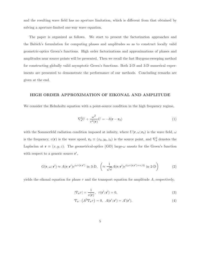
and the resulting wave field has no aperture limitation, which is different from that obtained by
solving a aperture-limited one-way wave equation.
The paper is organized as follows. We start to present the factorization approaches and
the Babich’s formulation for computing phases and amplitudes so as to construct locally valid
geometric-optics Green’s functions. High order factorizations and approximations of phases and
amplitudes near source points will be presented. Then we recall the fast Huygens-sweeping method
for constructing globally valid asymptotic Green’s functions. Both 2-D and 3-D numerical exper-
iments are presented to demonstrate the performance of our methods. Concluding remarks are
given at the end.
HIGH ORDER APPROXIMATION OF EIKONAL AND AMPLITUDE
We consider the Helmholtz equation with a point-source condition in the high frequency regime,
∇2rU +
ω2
v2(r)U = −δ(r− r0) (1)
with the Sommerfeld radiation condition imposed at infinity, where U(r, ω; r0) is the wave field, ω
is the frequency, v(r) is the wave speed, r0 ≡ (x0, y0, z0) is the source point, and ∇2r denotes the
Laplacian at r ≡ (x, y, z). The geometrical-optics (GO) large-ω ansatz for the Green’s function
with respect to a generic source r′,
G(r, ω; r′) ≈ A(r; r′)eiωτ(r;r′) in 3-D,
(
≈ 1√ωA(r; r′)ei(ωτ(r;r
′)+π/4) in 2-D
)
(2)
yields the eikonal equation for phase τ and the transport equation for amplitude A, respectively,
|∇rτ | =1
v(r), τ(r′; r′) = 0, (3)
∇r ·(
A2∇rτ)
= 0, A(r′; r′) = A′(r′). (4)
5

Since τ and A are locally smooth in a neighborhood of the source r′ excluding the source itself
(Milnor, 1963; Symes and Qian, 2003), they yield a valid GO Green’s function in that local neigh-
borhood. τ and A are weakly coupled in the sense that τ must be computed first by solving the
eikonal equation (3) and then substituted in the transport equation (4) for computing A. Since
the Laplacian of τ is involved in (4), in order to get l-th order accurate A, at least (l+ 2)-th order
accurate τ is required. Due to the source singularity as τ behaves like a distance function which
is non-differentiable at the source point (Qian and Symes, 2002a), computing high-order accurate
τ and A by finite-differencing equations (3) and (4) is not a trivial matter. Without special treat-
ments of source singularities, any high-order finite-difference methods for solving (3) and (4) can
formally have at most first-order accuracy and large errors.
High-order factorization for eikonals
We first recall a factorization approach to resolving the source singularity for computing τ (Pica,
1997; Zhang et al., 2005; Fomel et al., 2009; Luo and Qian, 2011, 2012; Luo et al., 2012). In the
factorization approach, τ is factored as
τ = τ τ , (5)
where τ is pre-determined analytically to capture the source singularity such that τ is the new
unknown that is smooth at the source and satisfies the factored eikonal equation,
|τ∇rτ + τ∇rτ | = 1/v(r). (6)
For instance, τ may be taken as τ(r; r′) = |r−r′|
v(r′) .
Since τ is smooth at the source, we can solve equation (6) efficiently with high-order Lax-
Friedrichs weighted essentially non-oscillatory (LxF-WENO) schemes as designed in (Kao et al.,
2004; Zhang et al., 2006; Luo and Qian, 2011; Luo et al., 2012). In a P -th order LxF-WENO finite
difference method on a mesh of size h, τ must be initialized in a neighborhood of size 2(P − 1)h
6

centered at the source, and these initial values are fixed during iterations. In Luo et al. (2014b), an
accurate, efficient, and systematic approach was introduced to initialize τ near the source. Based
on the power series expansion of τ2 which is smooth near the source, one can derive approximations
of τ near the source up to arbitrary order of accuracy.
We recall the derivation of high order approximation of τ near the source. Assume that T (r) ≡
τ2(r) and S(r) ≡ 1/v2(r) are analytic at the source which is set to be the origin without loss of
generality. We can expand T and S as power series,
T (r) =
∞∑
ν=0
Tν(r), S(r) =
∞∑
ν=0
Sν(r), (7)
where Tν and Sν are homogeneous polynomials of degree ν in r. From the eikonal equation (3), we
have
ST =1
4|∇rT |2. (8)
By substituting (7) into (8), we have
(
∞∑
ν=0
Sν(r)
)(
∞∑
ν=0
Tν(r)
)
=1
4
(
∞∑
ν=0
∇rTν(r)
)2
, (9)
from which one can derive Tν term by term by collecting terms of the same degree. Following
Luo et al. (2014b), we can derive
T0(r) = 0, T1(r) = 0, T2(r) = S0r2,
and a recursive formula for computing TP (r) for P ≥ 3,
(P − 1)S0 TP (r) =
P−2∑
ν=1
Sν(r)TP−ν(r)−1
4
P−2∑
ν=2
∇rTν+1(r) · ∇rTP−ν+1(r). (10)
Then we use the truncated sum TP ≡∑Pν=2 Tν to approximate T near the source, and we further
7

choose τP ≡√
TP to approximate τ near the source with accuracy
|τ(r)− τP (r)| = O(|r|P ), |r| → 0.
Taking τP as high-order approximations of τ near the source, we apply high-order LxF-WENO
methods to solve the factored equation (6). In the P -th order LxF-WENO method for solving (6)
to obtain τ , we first choose τ(r) ≡√S0|r|. To initialize τ near the source, τ is assigned as 1 at the
source and as τP /τ at other points in the 2(P −1)h neighborhood of the source so that these values
are fixed during the LxF-WENO sweeping iterations. At other points, the LxF-WENO iterations
are used to update τ with τ(r) ≡√S0|r|.
High-order factorization for amplitudes
We extend the above factorization approach to deal with the amplitude A near the source. Since
A is singular at the source, we introduce Babich’s formulation (Babich, 1965),
B = Aτ (d−1)/2 (11)
into the transport equation (4) for A so that we have the Babich’s transport equation for the
amplitude factor B (Babich, 1965),
∇rT (r) · ∇rB(r) +B(r)
[
1
2∇2
rT (r)− d/v2(r)
]
= 0, (12)
where d is the spatial dimension and T (r) = τ2(r). Since the amplitude factor B is smooth near
and at the source (Babich, 1965) while the original amplitude A is singular at the source, we will
use this transport equation to derive high order approximations of B near the source. In addition
8

to power series expansions in (7), we assume that B’s power series expansion is given as
B(r) =
∞∑
ν=0
Bν(r), (13)
where Bν are homogeneous polynomials of degree ν in r. It follows that Bν can be determined
term by term by substituting (13) into (12):
(
∞∑
ν=2
∇rTν(r)
)
·(
∞∑
ν=1
∇rBν(r)
)
+
(
∞∑
ν=0
Bν(r)
)[
1
2
(
∞∑
ν=2
∇2rTν(r)
)
− d
(
∞∑
ν=0
Sν(r)
)]
= 0. (14)
We know from Babich (1965) that
B0 =1
2√2π
for d = 2, and B0 =
√S0
4πfor d = 3.
Comparing the linear terms in (14) and using the homogeneity of B1, we have
∇rT2 · ∇rB1 +1
2(B0∇2
rT3 +B1∇2rT2)− d(B0S1 +B1S0) = 0,
⇒ 2S0r · ∇rB1 +1
2(B0∇2
rT3 + 2B1dS0)− d(B0S1 +B1S0) = 0,
⇒ 2S0B1 +1
2B0∇2
rT3 − dB0S1 = 0,
⇒ B1 =1
2S0
(
−1
2B0∇2
rT3 + dB0S1
)
.
(15)
Comparing the quadratic terms, we have
∇rT2 · ∇rB2 +∇rT3 · ∇rB1 +1
2(B0∇2
rT4 +B1∇2rT3 +B2∇2
rT2)− d(B0S2 +B1S1 +B2S0) = 0,
⇒ 2S0r · ∇rB2 +∇rT3 · ∇rB1 +1
2(B0∇2
rT4 +B1∇2
rT3 + 2B2dS0)− d(B0S2 +B1S1 +B2S0) = 0,
⇒ 2S02B2 +∇rT3 · ∇rB1 +1
2(B0∇2
rT4 +B1∇2rT3)− d(B0S2 +B1S1) = 0,
⇒ B2 =1
4S0
(
−∇rT3 · ∇rB1 −1
2(B0∇2
rT4 +B1∇2
rT3) + d(B0S2 +B1S1)
)
.
(16)
9

Equating P -th degree terms on both sides of (14), we have
BP =1
2PS0
(
−P−1∑
ν=1
∇rBν(r) · ∇rTP+2−ν(r)−1
2
P−1∑
ν=0
Bν(r)∇2rTP+2−ν(r) + d
P−1∑
ν=0
B0(r)SP−ν(r)
)
.
(17)
Consequently, we can now use the truncated sum to approximate B, i.e.,
BP ≡P∑
ν=0
Bν , (18)
and
|BP −B| = O(|r|P ), |r| → 0.
Taking BP as high-order approximation of B near the source, we will apply high-order LxF-
WENO methods to solve the Babich’s transport equation (12) for B. In the P -th order LxF-WENO
method for solving (12), B is assigned as BP in the 2(P − 1)h-neighborhood of the source so that
these values are fixed during the LxF-WENO iterations; at other points, the LxF-WENO iterations
are used to update B.
Comparing to the adaptive mesh refinement method for treating the source singularity used in
Kim and Cook (1999); Qian and Symes (2002a), high-order factorization based high-order LxF-
WENO sweeping methods make computing high-order accurate τ and B easy and efficient, resulting
in high-order accurate τ and A and locally valid first-arrival Green’s functions. If one is satisfied
with accurate first-arrival Green’s functions, then the schemes developed above suffice. However,
since in genereal one needs multi-arrival Green’s functions, we incorporate these first-arrival Green’s
functions into the fast Huygens sweeping method introduced in Luo et al. (2014a) to build globally
valid multi-arrival Green’s functions.
10

HUYGENS-PRINCIPLE BASED GLOBALLY VALID GREEN’S
FUNCTIONS
Assume that a domain Ω is illuminated by an exterior source r0 /∈ Ω, and S = ∂Ω is the closed
surface enclosing the domain Ω; see Figure 1(a). At any observation point r ∈ Ω, the wave field
U(r; r0) excited by the source r0 can be written as the Huygens-Kirchhoff (HK) integral over S
(Burridge, 1962; Baker and Copson, 1987):
U(r; r0) =
∫
S
G(r′; r)∇r′U(r′; r0) · n(r′)− U(r′; r0)∇r′G(r′; r) · n(r′)
dS(r′)
=
∫
S
G(r; r′)∇r′U(r′; r0) · n(r′)− U(r′; r0)∇r′G(r; r′) · n(r′)
dS(r′),
(19)
where G(r; r′) = G(r′; r) by reciprocity, n(r′) is the outward normal to S at r′ = (x′, y′, z′),
and G(r; r′) is the Green’s function associated with the source r′. In the integral, G(r; r′) and
∇r′G(r; r′) · n(r′) associated with r′ on S can be approximated with the GO ansatz (2).
By retaining the leading order term after substituting (2) into (19), we have
U(r; r0) ≈∫
S
G(r; r′)[
∇r′U(r′; r0) · n(r′)]
−G(r; r′)∇r′τ(r; r′) · n(r′)
[
iωU(r′; r0)]
dS(r′)
≈∫
S
G(r; r′)[
∇r′U(r′; r0) · n(r′)]
−G(r; r′) cos(θ(r; r′))[
iωU(r′; r0)/v(r′)]
dS(r′),
(20)
where θ is the takeoff angle of the ray from source r′ to receiver r and is constant along the ray,
i.e.,
∇rθ(r; r′) · ∇rτ(r; r
′) = 0; (21)
consequently,
∇r cos(θ(r; r′)) · ∇rτ(r; r
′) = 0. (22)
Since the first-arrival GO approximations of Green’s functions associated with the secondary sources
are valid only locally, (20) can only be used in a narrow band near S so that rays emanating from
the source have not developed caustics yet. Hence the fast Huygens sweeping method carries out
11

the integration (20) in a layer by layer manner; see Figure 1(b) and Figure 2. The secondary sources
are placed on the boundary of each layer, and the HK integral (20) is performed inside each layer.
Layer-based Huygens sweeping
We recall the planar-layer based Huygens sweeping method (Luo et al., 2014a) as illustrated in
Figure 1(b) and Figure 2 and summarized as follows.
Algorithm: Algorithmic sketch for Huygens sweeping method
• Stage 1 (offline). Precompute asymptotic ingredients such as phases, amplitudes, and
takeoff angles. Since these ingredients only depend on the velocity and do not depend on
wavelength or frequency, these can be computed on very coarse meshes by using high-order
schemes. We carry out the following steps: (1) the whole computational domain is parti-
tioned into layers as in Figure 1(b) so that rays emanating from the primary source and each
secondary source have not developed caustics yet; (2) the tables of phases, amplitudes and
takeoff angles with respect to the primary source in the first layer (see Figure 2(a)) and those
tables for each secondary source located on the layer boundary of the other layers (see Fig-
ure 2(b)) are computed by solving the relevant equations as described above with high-order
LxF-WENO methods in the corresponding layer; and (3) these tables are compressed with
the Chebyshev expansion based data compression technique (Alkhalifah, 2011; Boyd, 2001;
Luo et al., 2014a); see Appendix A.
• Stage 2 (online). Given a frequency ω, we specify four to six (4 to 6) points per wavelength
so that the wavefield is sampled with n mesh points along each dimension: (1) in the first
layer containing the primary source, construct the first-arrival Green’s function with tables
of the primary source; see Figure 2(a); (2) from the second layer to all the other layers, for
each line of secondary sources on the layer boundary, tables of phases, amplitudes and takeoff
angles are read from the hard drive and used to reconstruct the tables on the underlying
12

mesh by Chebyshev sums (see Appendix A); if necessary the tables are interpolated with
respect to the secondary sources onto the underlying mesh; and (3) the HK integral (20) is
then discretized with a numerical quadrature rule, such as the trapezoidal rule as used in
the current work, and the resulting matrix-vector products are evaluated by a fast butterfly
algorithm as shown in Luo et al. (2014a); see Figure 2(b).
Complexity analysis
In the above algorithm, two sets of different meshes are involved in the computation. One set of
meshes is used for computing GO ingredients; since these ingredients are independent of wavelength
or frequency, these meshes are independent of wavelength as well and can be very coarse so that
high-order schemes still can yield sufficiently accurate GO ingredients. The other set of meshes
is used to sample the wavefield. Since we need to specify four to six points per wavelength to
resolve wave oscillations, these meshes depend on wavelength or frequency. Therefore, the following
complexity analysis treats the two sets of meshes differently.
Assume that there are L layers in the partition. In Stage 1, the complexity of computing each
table in each layer with LxF-WENO methods is O(md−1(m/L) logm), where m mesh points are
used for each spatial direction. Since there are O(md−1) secondary sources for each layer, the total
complexity of computing all the tables for secondary sources is LO(md−1(md−1(m/L) logm)) =
O(m2d−1 logm), which is analogous to the computational complexity for asymptotic ingredients in
phase space (Symes and Qian, 2003; Leung et al., 2007; Luo et al., 2014a). Since these tables are
precomputed and are independent of wavelength or frequency, those tables can be computed on
very coarse meshes by using high-order schemes and can be reused for different frequencies.
In Stage 2, direct evaluation of the HK-integral induced matrix-vector products is computa-
tionally expensive. To accelerate the evaluation, we adapt a multilevel matrix decomposition based
butterfly algorithm originated in Michielssen and Boag (1996) and further developed in O’Neil
(2007); Ying (2009); Candes et al. (2009); Demanet et al. (2012); Hu et al. (2013); Luo et al.
13

(2014a). Following Luo et al. (2014a), given frequency ω, four to six points are specified per wave-
length so that the wavefield is sampled with n mesh points along each spatial direction. For each
layer, the complexity of the butterfly algorithm is O(nd−1(n/L) log(nd−1(n/L))) = O((N/L) logN),
where N = O(nd) and the prefactor is independent of frequency ω; the complexity of Chebyshev
sums and interpolation with respect to secondary sources is O(N/L), where the prefactor depends
on the number of spectral coefficients in the truncated Chebyshev expansion. The number of spec-
tral coefficients is considered to be much smaller than O(n). Therefore, the total complexity of
constructing the wavefield in the whole domain is O(N logN). Please refer to Luo et al. (2014a)
for more implementation details of the fast butterfly algorithm used here.
Once the data tables are pre-computed, the fast Huygens sweeping method can be used to
construct the global wave field with O(N logN) complexity for a given primary source and for an
arbitrary given frequency. Moreover, the data tables can be reused for many different primary
sources. For different primary sources, only the tables with respect to the primary sources inside
the first layer are recomputed. The tables of the other layers are reused. Therefore, we refer
Stage 1 as “offline” and Stage 2 as “online”. These unique merits are much desired in many
applications, such as seismic imaging and inversion.
NUMERICAL EXAMPLES
We present several numerical experiments to demonstrate our new method. We denote the coarse
mesh in Stage 1 as GO mesh. We choose P = 3 in the high-order factorization for computing τ and
B. The mesh for sampling wavefields is chosen such that a fixed number of points (4 to 6 points)
per wavelength are used to resolve wave oscillations. We compare our numerical solutions with
those obtained by a direct solver on a much finer mesh. For the direct finite-difference Helmholtz
solver, we use a nine-point stencil (Jo et al., 1996) instead of the usual five-point stencil to reduce
dispersion errors and obtain more reliable wave fields; the perfectly-matched-layer (PML) absorbing
boundary conditions are also imposed (Berenger, 1994). The resulting sparse linear system is solved
14
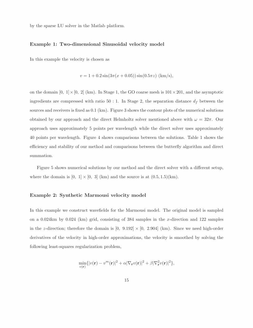
by the sparse LU solver in the Matlab platform.
Example 1: Two-dimensional Sinusoidal velocity model
In this example the velocity is chosen as
v = 1 + 0.2 sin(3π(x + 0.05)) sin(0.5πz) (km/s),
on the domain [0, 1]× [0, 2] (km). In Stage 1, the GO coarse mesh is 101×201, and the asymptotic
ingredients are compressed with ratio 50 : 1. In Stage 2, the separation distance df between the
sources and receivers is fixed as 0.1 (km). Figure 3 shows the contour plots of the numerical solutions
obtained by our approach and the direct Helmholtz solver mentioned above with ω = 32π. Our
approach uses approximately 5 points per wavelength while the direct solver uses approximately
40 points per wavelength. Figure 4 shows comparisons between the solutions. Table 1 shows the
efficiency and stability of our method and comparisons between the butterfly algorithm and direct
summation.
Figure 5 shows numerical solutions by our method and the direct solver with a different setup,
where the domain is [0, 1]× [0, 3] (km) and the source is at (0.5, 1.5)(km).
Example 2: Synthetic Marmousi velocity model
In this example we construct wavefields for the Marmousi model. The original model is sampled
on a 0.024km by 0.024 (km) grid, consisting of 384 samples in the x-direction and 122 samples
in the z-direction; therefore the domain is [0, 9.192] × [0, 2.904] (km). Since we need high-order
derivatives of the velocity in high-order approximations, the velocity is smoothed by solving the
following least-squares regularization problem,
minv(r)
|v(r)− vm(r)|2 + α|∇rv(r)|2 + β|∇2rv(r)|2,
15

where vm is the original Marmousi model, α and β are smoothness parameters. We choose α = β =
10−4. Figure 6 shows the Marmousi models. We first test a case with the smoothed velocity. The
velocity field is a sampled window from receivers 218 to 313 (96 receivers in total) in the smoothed
Marmousi model. The windowed domain is [5.208, 7.488] × [0, 2.904] (km). In Stage 1, the GO
coarse mesh is 96× 122 and the asymptotic ingredients are compressed with ratio 25 : 1. In Stage
2, the separation distance df between the sources and receivers is fixed as 0.192 (km). We apply
our new algorithm to the smoothed Marmousi velocity model as in Figure 6(b). This synthetic
geological structure creates many strong and localized velocity heterogeneities. Figure 7 shows the
wave fields with the primary source point given as (5.380, 0.24) (km) and ω = 32π by two different
methods, where the fast Huygens sweeping method uses a mesh of 286× 364 points and the direct
Helmholtz solver uses a mesh of 1711 × 2179 points. To apply the direct Helmholtz solver on the
fine mesh, the velocity field on the original coarse mesh is interpolated onto the finer mesh first
with spline interpolations.
Next we choose a sampled window from receivers 41 to 158 of the Marmousi model where the
velocity is only slightly smoothed; see Figure 8. The windowed domain is [0, 2.904]× [0.96, 3.768]
(km). In Stage 1, the GO coarse mesh is 118× 122 and the data compression ratio for asymptotic
ingredients is 25 : 1. In Stage 2, the separation distance df between the sources and receivers
is fixed as 0.192 (km). Figure 9 shows the wave fields with the primary source point given as
(1.488, 0.48) (km) and ω = 32π by the two methods, where the fast Huygens sweeping method
uses a mesh of 352× 364 points and the direct Helmholtz solver uses a mesh of 2107× 2179 points.
To apply the direct Helmholtz solver on the fine mesh, the velocity field on the original coarse mesh
is interpolated onto the finer mesh first with spline interpolations.
16

Example 3: Three-dimensional Vinje velocity model (Vinje et al., 1996)
In the example the velocity is chosen as
v = 3.0 − 1.75e(−((x−1)2+(y−1)2+(z−1)2)/0.64) (km/s),
on the domain [0, 2] × [0, 2] × [0, 2] (km). In Stage 1, the GO coarse mesh is 51 × 51 × 51, and
the data compression ratio for asymptotic ingredients is 32 : 1. In Stage 2, the separation distance
df between the sources and receivers is fixed as 0.3 (km).
We partition the 3-D domain into two layers at the plane z = 1.2 (km). When ω = 32π, there
are roughly 26 waves propagating in each direction. If a direct solver is used to compute the wave
field, then the number of unknowns is roughly 17 millions if 10 points per wavelength is used to
capture each wave, resulting in a huge linear system to deal with, not to mention the fact that
whether 10 points per wavelength suffice or not. To use our fast Huygens sweeping method, we
choose approximately 4 points per wavelength.
Figure 10 shows the results for different primary sources. The tables corresponding to the
primary source in first layer need to be recomputed for different primary sources. Tables with
respect to those secondary sources do not need to be recomputed. Table 2 shows the running times
of our method for different ω’s.
CONCLUSION
We have developed the fast Huygens sweeping method for evaluating the Huygens-Kirchhoff in-
tegral so that locally valid first-arrival Green’s functions can be integrated into a globally valid
multi-arrival Green’s function. The needed ingredients for constructing first-arrival Green’s func-
tions, such as first-arrival traveltimes and amplitudes, were computed by utilizing a set of newly
developed tools, such as the factorization approach, the Babich’s formulation, power-series based
high-order approximations, and high-order LxF-WENO methods. The Huygens-Kirchhoff integral
17

were evaluated by adapting a fast butterfly algorithm so that the fast Huygens sweeping method has
computational complexity O(N logN), where N is the total number of mesh points, and the pro-
portionality constant depends on the desired accuracy and is independent of frequency. Numerical
examples demonstrated performance, efficiency, and accuracy of the proposed method.
ACKNOWLEDGMENT
The authors would like to thank the reviewers and associate editors for comments that improve
this work. Qian is supported by NSF-1222368. Luo is supported by NSF DMS-1418908.
18

APPENDIX A
COMPRESSION WITH CHEBYSHEV EXPANSION
We illustrate the compression process for a 3-D traveltime table. The same can be done for
amplitude and takeoff angle tables, and for 2-D tables (Boyd, 2001; Alkhalifah, 2011). Without
loss of generality, we assume that the traveltime τ(r; r0) is defined on [−1, 1]3 for a given source
point r0. τ can be expanded in terms of Chebyshev polynomials of the first kind (Boyd, 2001),
τ(r; r0) = τ(x, y, z; r0) =
∞∑
m=0
∞∑
n=0
∞∑
k=0
Cmnk(r0)Tm(x)Tn(y)Tk(z), (A-1)
where Tl(·) is the Chebyshev polynomial of the first kind and of order l: Tl(·) = cos(l cos−1(·)); and
Cmnk(r0) are spectral coefficients. To determine Cmnk(r0), we use the computed traveltime on
the coarse mesh in Stage 1. Cmnk(r0) are then computed with the fast Fourier cosine transform
(Boyd, 2001; Alkhalifah, 2011). In numerical applications, for given accuracy it is enough to keep
only the first few coefficients among Cmnk(r0),
τ(r; r0) = τ(x, y, z; r0) ≈CX−1∑
m=0
CY −1∑
n=0
CZ−1∑
k=0
Cmnk(r0)Tm(x)Tn(y)Tk(z), (A-2)
with CX , CY and CZ being given numbers. Instead of saving τ on the coarse mesh, the set of
significant coefficients,
C = Cmnk(r0) : 0 ≤ m ≤ CX − 1, 0 ≤ n ≤ CY − 1, 0 ≤ k ≤ CZ − 1,
will be saved for later use. In practice, it is possible to reconstruct τ with high accuracy even with
a relatively high compression ratio defined as (the size of the coarse mesh)/(CXCY CZ).
With C, the traveltime on any specified computational mesh can be computed by evaluating
the formula (A-2) on that mesh as product of low-rank matrices, which is detailed below by using
Matlab notation:
19

• In 3-D, τ on a mesh of size M × N ×K spanned by X = [−1 : hx : 1], Y = [−1 : hy : −1],
and Z = [−1 : hz : 1] is reconstructed by
τ = permute(permute(T′XCTZ, [1 3 2])TY, [1 3 2]),
where TX, TY, and TZ are of size CX ×M , CY ×N , and CZ ×K respectively, and
TX(l, :) = Tl−1(X), TY(l, :) = Tl−1(Y), and TZ(l, :) = Tl−1(Z).
• In 2-D, τ on a 2-D mesh of size M ×K spanned by X = [−1 : hx : 1] and Z = [−1 : hz : 1] is
reconstructed as
τ = T′XCTZ,
where C is of size CX × CZ .
20

REFERENCES
Albertin, U., D. Yingst, P. Kitchenside, and V. Tcheverda, 2004, True-amplitude beam migration,
in 74th Ann. Internat. Mtg., Soc. Expl. Geophys., Expanded Abstracts: Soc. Expl. Geophys.,
949–952.
Alkhalifah, T., 2011, Efficient traveltime compression for 3D prestack Kirchhoff migration: Geo-
phys. Prosp., 69, 1–9.
Alkhalifah, T., and S. Fomel, 2010, An eikonal-based formulation for traveltime perturbation with
respect to the source location: Geophysics, 75, T175–T183.
Babich, V. M., 1965, The short wave asymptotic form of the solution for the problem of a point
source in an inhomogeneous medium: USSR Computational Mathematics and Mathematical
Physics, 5, 247–251.
Babuska, I. M., and S. A. Sauter, 2000, Is the pollution effect of the FEM avoidable for the
Helmholtz equation considering high wave numbers?: SIAM Review, 42, 451–484.
Baker, B., and E. T. Copson, 1987, The mathematical theory of Huygens’ principle: Ams Chelsea
Publishing.
Bao, G., J. Lai, and J. Qian, 2014, Fast multiscale Gaussian beam methods for wave equations in
bounded domains: J. Comput. Phys., 261, 36–64.
Benamou, J. D., S. Luo, and H.-K. Zhao, 2010, A Compact Upwind Second Order Scheme for the
Eikonal Equation: J. Comput. Math., 28, 489–516.
Berenger, J.-P., 1994, A perfectly matched layer for the absorption of electromagnetic waves: J.
Comput. Phys., 114, 185–200.
Berryhill, J. R., 1979, Wave-equation datuming: Geophysics, 44, 1329–1344.
Bevc, D., 1997, Imaging complex structures with semirecursive Kirchhoff migration: Geophysics,
62, 577–588.
Boyd, J. P., 2001, Chebyshev and Fourier Spectral Methods: Second edition, Dover, New York.
Burridge, R., 1962, The reflexion of high-frequency sound in a liquid sphere: Proc. Roy. Soc. Ser.
A, 270, 144–154.
21
Candes, E., L. Demanet, and L. Ying, 2009, A fast butterfly algorithm for the computation of
Fourier integral operators: Multiscale Modeling & Simulation, 7, 1727–1750.
Cerveny, V., I. A. Molotkov, and I. Psencik, 1977, Ray method in seismology: Univerzita Karlova
press.
Cerveny, V., M. Popov, and I. Psencik, 1982, Computation of wave fields in inhomogeneous media-
Gaussian beam approach: Geophys. J. R. Astr. Soc., 70, 109–128.
Chapman, C. H., 1985, Ray theory and its extensions: WKBJ and Maslov seismogram: J. Geophys.,
58, 27–43.
Demanet, L., M. Ferrara, N. Maxwell, J. Poulson, and L. Ying, 2012, A butterfly algorithm for
synthetic aperture radar imaging: SIAM J. Imaging Sci., 5, 203–243.
Fomel, S., S. Luo, and H.-K. Zhao, 2009, Fast sweeping method for the factored eikonal equation:
J. Comput. Phys., 228, 6440–6455.
Franklin, J., and J. M. Harris, 2001, A high-order fast marching scheme for the linearized eikonal
equation: J. Comput. Acoustics, 9, 1095–1109.
Geoltrain, S., and J. Brac, 1993, Can we image complex structures with first-arrival traveltime:
Geophysics, 58, 564–575.
Gray, S., 2005, Gaussian beam migration of common shot records: Geophysics, 70, S71–S77.
Gray, S., and W. May, 1994, Kirchhoff migration using eikonal equation traveltimes: Geophysics,
59, 810–817.
Hill, N., 1990, Gaussian beam migration: Geophysics, 55, 1416–1428.
Hole, J., and B. C. Zelt, 1995, 3-D finite-difference reflection traveltimes: Geophys. J. Internat.,
121, 427–434.
Hu, C., and P. Stoffa, 2009, Slowness-driven Gaussian-beam prestack depth migration for low-fold
seismic data: Geophysics, 74, WCA35–WCA45.
Hu, J., S. Fomel, L. Demanet, and L. Ying, 2013, A fast butterfly algorithm for generalized Radon
transforms: Geophysics, 78, U41–U51.
Jo, C.-H., C. Shin, and J. H. Suh, 1996, An optimal 9-point, finite-difference, frequency-space, 2-D
22

scalar wave extrapolator: Geophysics, 61, 529–537.
Kao, C. Y., S. Osher, and J. Qian, 2004, Lax-Friedrichs sweeping schemes for static Hamilton-Jacobi
equations: J. Comput. Phys., 196, 367–391.
Kim, S., and R. Cook, 1999, 3-D traveltime computation using second-order ENO scheme: Geo-
physics, 64, 1867–1876.
Leung, S., and J. Qian, 2006, An adjoint state method for three-dimensional transmission traveltime
tomography using first-arrivals: Comm. Math. Sci., 4, 249–266.
——–, 2010, The backward phase flow and FBI-transform-based Eulerian Gaussian beams for the
Schrodinger equation: J. Comput. Phys., 229, 8888–8917.
Leung, S., J. Qian, and R. Burridge, 2007, Eulerian Gaussian beams for high-frequency wave
propagation: Geophysics, 72, SM61–SM76.
Li, S., and S. Fomel, 2013, Kirchhoff migration using eikonal-based computation of traveltime
source derivative: Geophysics, 78, S211–S219.
Luo, S., and J. Qian, 2011, Factored singularities and high-order Lax-Friedrichs sweeping schemes
for point-source traveltimes and amplitudes: J. Comput. Phys., 230, 4742–4755.
——–, 2012, Fast sweeping methods for factored anisotropic eikonal equations: multiplicative and
additive factors: J. Sci. Comput., 52, 360–382.
Luo, S., J. Qian, and R. Burridge, 2014a, Fast Huygens sweeping methods for Helmholtz equations
in inhomogeneous media in the high frequency regime: J. Comput. Phys., 270, 378–401.
——–, 2014b, High-order factorization based high-order hybrid fast sweeping methods for point-
source Eikonal equations: SIAM J. Numer. Anal., 52, 23–44.
Luo, S., J. Qian, and H.-K. Zhao, 2012, Higher-order schemes for 3-D traveltimes and amplitudes:
Geophysics, 77, T47–T56.
Michielssen, E., and A. Boag, 1996, A multilevel matrix decomposition algorithm for analysing
scattering from large structures: IEEE Trans. Antennas Propagat., 44, no. 8, 1086–1093.
Milnor, J., 1963, Morse Theory: Princeton Univ. Press.
Nichols, D., 1994, Imaging complex structures using band limited Green’s functions: PhD thesis,
23

Stanford University, Stanford, CA94305.
O’Neil, M., 2007, A new class of analysis-based fast transforms: Doctoral Dissertation, Yale Uni-
versity.
Operto, S., S. Xu, and G. Lambare, 2000, Can we image quantitatively complex models with rays:
Geophysics, 65, 1223–1238.
Pica, A., 1997, Fast and accurate finite-difference solutions of the 3D eikonal equation parametrized
in celerity: 67th Ann. Internat. Mtg, Soc. of Expl. Geophys., 1774–1777.
Popov, M. M., 1982, A new method of computation of wave fields using Gaussian beams: Wave
Motion, 4, 85–97.
Qian, J., and W. W. Symes, 2002a, An adaptive finite-difference method for traveltimes and am-
plitudes: Geophysics, 67, 167–176.
——–, 2002b, Finite-difference quasi-P traveltimes for anisotropic media: Geophysics, 67, 147–155.
Qian, J., and L. Ying, 2010a, Fast Gaussian wavepacket transforms and Gaussian beams for the
Schrodinger equation: J. Comput. Phys., 229, 7848–7873.
——–, 2010b, Fast multiscale Gaussian wavepacket transforms and multiscale Gaussian beams for
the wave equation: SIAM J. Multiscale Modeling and Simulation, 8, 1803–1837.
Qian, J., Y.-T. Zhang, and H.-K. Zhao, 2007a, A fast sweeping methods for static convex Hamilton-
Jacobi equations: J. Sci. Comput., 31(1/2), 237–271.
——–, 2007b, Fast sweeping methods for eikonal equations on triangulated meshes: SIAM J.
Numer. Anal., 45, 83–107.
Qin, F., Y. Luo, K. B. Olsen, W. Cai, and G. T. Schuster, 1992, Finite difference solution of the
eikonal equation along expanding wavefronts: Geophysics, 57, 478–487.
Ralston, J., 1983, Gaussian beams and the propagation of singularities. Studies in partial differential
equations. MAA Studies in Mathematics, 23. Edited by W. Littman. pp.206-248.
Schneider, W. A. J., 1995, Robust and efficient upwind finite-difference traveltime calculations in
three dimensions: Geophysics, 60, 1108–1117.
Schneider, W. A. J., K. Ranzinger, A. Balch, and C. Kruse, 1992, A dynamic programming ap-
24

proach to first arrival traveltime computation in media with arbitrarily distributed velocities:
Geophysics, 57, 39–50.
Serna, S., and J. Qian, 2010, A stopping criterion for higher-order sweeping schemes for static
Hamilton-Jacobi equations: J. Comput. Math., 28, 552–568.
Sethian, J. A., and A. M. Popovici, 1999, 3-D traveltime computation using the fast marching
method: Geophysics, 64, 516–523.
Symes, W. W., and J. Qian, 2003, A slowness matching Eulerian method for multivalued solutions
of eikonal equations: J. Sci. Comp., 19, 501–526.
Tanushev, N., J. Qian, and J. Ralston, 2007, Mountain waves and Gaussian beams: SIAM J.
Multiscale Modeling and Simulation, 6, 688–709.
Tsai, Y.-H., L.-T. Cheng, S. Osher, and H.-K. Zhao, 2003, Fast sweeping algorithms for a class of
Hamilton-Jacobi equations: SIAM J. Numer. Anal., 41, 673–694.
van Trier, J., and W. W. Symes, 1991, Upwind finite-difference calculation of traveltimes: Geo-
physics, 56, 812–821.
Vidale, J. E., 1990, Finite-difference calculation of traveltimes in three dimensions: Geophysics,
55, 521–526.
Vinje, V., E. Iversen, K. Astebol, and H. Gjoystdal, 1996, Estimation of multivalued arrivals in 3d
models using wavefront construction - part I: Geophysical Prospecting, 44, 819–842.
Wang, S., M. V. de Hoop, and J. Xia, 2011, On 3D modeling of seismic wave propagation via a
structured parallel multifrontal direct Helmholtz solver: Geophys. Prosp., 59, 857–873.
Ying, L., 2009, Sparse Fourier transform via butterfly algorithm: SIAM J. Sci. Comput., 31,
1678–1694.
Zhang, L., J. W. Rector, and G. M. Hoversten, 2005, Eikonal solver in the celerity domain: Geo-
physical Journal International, 162, 1–8.
Zhang, Y. T., H. K. Zhao, and J. Qian, 2006, High order fast sweeping methods for static Hamilton-
Jacobi equations: J. Sci. Comp., 29, 25–56.
Zhao, H.-K., 2005, A fast sweeping method for eikonal equations: Math. Comput., 74, 603–627.
25

LIST OF FIGURES
1 2-D demonstration of HK integral and partition of domain into layers: (a) HK integral
with S an infinite plane; and (b) partition of domain into planar layers. Star represents the primary
source.
2 Receivers and sources in HK integral and illustration of the fast Huygens sweeping algo-
rithm. Larger star represents the primary source; little stars represent the secondary sources on the
boundary of each layer; and the grid represents the mesh. In offline Stage 1, coarse mesh is used.
In online Stage 2, refined mesh is used and depends on ω. The region of size df is independent of
ω. (a) shows the first layer with respect to the primary source; and (b) shows a layer l with l > 1
and with respect to secondary sources on the boundary of this layer.
3 Sinusoidal model. Real part of the wave field with (a) obtained by our method (mesh
101 × 201, solid black lines indicate the locations of secondary sources for each layer); and (b) ob-
tained by the direct Helmholtz solver (mesh 801× 1601). ω = 32π. Source point is (0.5, 0.2)(km).
4 Sinusoidal model. Real part of the wave field and (a)-(d) are comparisons between the
solutions obtained by our method and the direct Helmholtz solver at z = 0.55, 1.15, 1.45, 1.75
(km), respectively. Solid lines represent solutions by the direct Helmholtz solver; Circles represent
solutions by our method (p = 9). ω = 32π. Source point is (0.5, 0.2)(km).
5 Sinusoidal model. Real part of the wave field with (a) obtained by our method (mesh
101 × 301, solid black lines indicate the locations of secondary sources for each layer); and (b) ob-
tained by the direct Helmholtz solver (mesh 801× 2401). ω = 32π. Source point is (0.5, 1.5)(km).
6 Marmousi model with (a) the original Marmousi velocity field; and (b) the smoothed ve-
locity field. The region between two black lines is the sampled window from receivers 218 to 313.
7 Smoothed Marmousi model with velocity in Figure 6. Real part of the wave field with (a)
obtained by our method; and (b) obtained by the direct Helmholtz solver. Solid lines show the
positions of the secondary sources. (c)-(d) are comparisons of the solutions at z = 1.472, 2.592(km)
respectively, where circles represent the solution by our method and solid lines represent the solu-
tion by the direct Helmholtz solver.
26

8 Marmousi model with (a) the original Marmousi velocity field; and (b) slightly smoothed
velocity field. The region between two black lines is the sampled window from receivers 41 to 158.
9 Smoothed Marmousi model with velocity in Figure 8. Real part of the wave field with (a)
obtained by our method; and (b) obtained by the direct Helmholtz solver. Solid lines show the
positions of the secondary sources. (c)-(d) are comparisons of the solutions at x = 2.640, 3.360(km)
respectively, where circles represent the solution by our method and solid lines represent the solu-
tion by the direct Helmholtz solver.
10 Vinje model. For (a)-(b)-(c), the primary point source is (0.6, 0.6, 0.24) (km); and for
(d)-(e)-(f), the primary source is (1.4, 1.4, 0.36) (km). (a)-(b)-(c) show the real part of the wave-
fields at x = 0.6(km), y = 0.6(km), and z = 1.8(km) respectively; and (d)-(e)-(f) show the real
part of the wavefields at x = 1.4(km), y = 1.4(km), and z = 1.8(km) respectively. Wavefields are
constructed by our method on a mesh 101 × 101× 101 with ω = 32π.
27

a)
0 0( , )x z
( ', ')x z
Ω
n
!
τ∇θ
( , )x z
S
z
b)
!"#$%&'!
!"#$%&(!
!"#$%&)!
!"#$%&*!
0 0( , )x z
z
Figure 1: 2-D demonstration of HK integral and partition of domain into layers: (a) HK integralwith S an infinite plane; and (b) partition of domain into planar layers. Star represents the primarysource.
28

a)
!"#$%&'!
z
fd
b)
!"#$%&&'&!
z
fd
fd
!"#$%&&'()&
!"#$%&&'*)&
Figure 2: Receivers and sources in HK integral and illustration of the fast Huygens sweepingalgorithm. Larger star represents the primary source; little stars represent the secondary sourceson the boundary of each layer; and the grid represents the mesh. In offline Stage 1, coarse mesh isused. In online Stage 2, refined mesh is used and depends on ω. The region of size df is independentof ω. (a) shows the first layer with respect to the primary source; and (b) shows a layer l withl > 1 and with respect to secondary sources on the boundary of this layer.
29

a) x(km)
z(km
)
0 0.5 1
0
0.5
1
1.5
2 −0.1
−0.05
0
0.05
0.1
b) x(km)
z(km
)
0 0.5 1
0
0.5
1
1.5
2 −0.1
−0.05
0
0.05
0.1
Figure 3: Sinusoidal model. Real part of the wave field with (a) obtained by our method (mesh101 × 201, solid black lines indicate the locations of secondary sources for each layer); and (b)obtained by the direct Helmholtz solver (mesh 801×1601). ω = 32π. Source point is (0.5, 0.2)(km).
30

a)0 0.5 1
−0.02
0
0.02
x(km)
Wav
efie
ld
b)0 0.5 1
−0.02
0
0.02
0.04
x(km)
Wav
efie
ld
c)0 0.5 1
−0.04
−0.02
0
0.02
0.04
x(km)
Wav
efie
ld
d)0 0.5 1
−0.02
−0.01
0
0.01
0.02
0.03
x(km)
Wav
efie
ldFigure 4: Sinusoidal model. Real part of the wave field and (a)-(d) are comparisons between thesolutions obtained by our method and the direct Helmholtz solver at z = 0.55, 1.15, 1.45, 1.75(km), respectively. Solid lines represent solutions by the direct Helmholtz solver; Circles representsolutions by our method (p = 9). ω = 32π. Source point is (0.5, 0.2)(km).
31

a) x(km)
z(km
)
0 0.5 1
0
1
2
3 −0.1
−0.05
0
0.05
0.1
b) x(km)
z(km
)
0 0.5 1
0
1
2
3 −0.1
−0.05
0
0.05
0.1
Figure 5: Sinusoidal model. Real part of the wave field with (a) obtained by our method (mesh101 × 301, solid black lines indicate the locations of secondary sources for each layer); and (b)obtained by the direct Helmholtz solver (mesh 801×2401). ω = 32π. Source point is (0.5, 1.5)(km).
32

a)
x(km)
z(km
)
0 2 4 6 8
012 2
4
b)
x(km)
z(km
)
0 2 4 6 8
012 2
4
Figure 6: Marmousi model with (a) the original Marmousi velocity field; and (b) the smoothedvelocity field. The region between two black lines is the sampled window from receivers 218 to 313.
33

a) x(km)
z(km
)
5.5 6 6.5 7
0
0.5
1
1.5
2
2.5
−0.1
−0.05
0
0.05
0.1
b) x(km)
z(km
)
5.5 6 6.5 7
0
0.5
1
1.5
2
2.5
−0.1
−0.05
0
0.05
0.1
c)5.5 6 6.5 7
−0.03
−0.02
−0.01
0
0.01
0.02
x(km)
Wav
efie
ld
d)5.5 6 6.5 7
−0.02
0
0.02
0.04
x(km)
Wav
efie
ldFigure 7: Smoothed Marmousi model with velocity in Figure 6. Real part of the wave field with(a) obtained by our method; and (b) obtained by the direct Helmholtz solver. Solid lines show thepositions of the secondary sources. (c)-(d) are comparisons of the solutions at z = 1.472, 2.592(km)respectively, where circles represent the solution by our method and solid lines represent the solutionby the direct Helmholtz solver.
34

a)
x(km)
z(km
)
0 2 4 6 8
012 2
4
b)
x(km)
z(km
)
0 2 4 6 8
012 2
4
Figure 8: Marmousi model with (a) the original Marmousi velocity field; and (b) slightly smoothedvelocity field. The region between two black lines is the sampled window from receivers 41 to 158.
35

a) x(km)
z(km
)
1 2 3
0
0.5
1
1.5
2
2.5
−0.1
−0.05
0
0.05
0.1
b) x(km)
z(km
)
1 2 3
0
0.5
1
1.5
2
2.5
−0.1
−0.05
0
0.05
0.1
c)0 1 2
−0.03
−0.02
−0.01
0
0.01
0.02
z(km)
Wav
efie
ld
d)0 1 2
−0.02
0
0.02
0.04
z(km)
Wav
efie
ldFigure 9: Smoothed Marmousi model with velocity in Figure 8. Real part of the wave field with(a) obtained by our method; and (b) obtained by the direct Helmholtz solver. Solid lines show thepositions of the secondary sources. (c)-(d) are comparisons of the solutions at x = 2.640, 3.360(km)respectively, where circles represent the solution by our method and solid lines represent the solutionby the direct Helmholtz solver.
36

a) y(km)z(
km)
0 1 2
0
0.5
1
1.5
2 −0.2
−0.1
0
0.1
0.2
b) x(km)
z(km
)
0 1 2
0
0.5
1
1.5
2 −0.2
−0.1
0
0.1
0.2
c) x(km)
y(km
)
0 1 2
0
0.5
1
1.5
2 −0.2
−0.1
0
0.1
0.2
d) y(km)
z(km
)
0 1 2
0
0.5
1
1.5
2 −0.2
−0.1
0
0.1
0.2
e) x(km)
z(km
)
0 1 2
0
0.5
1
1.5
2 −0.2
−0.1
0
0.1
0.2
f) x(km)
y(km
)
0 1 2
0
0.5
1
1.5
2 −0.2
−0.1
0
0.1
0.2
Figure 10: Vinje model. For (a)-(b)-(c), the primary point source is (0.6, 0.6, 0.24) (km); andfor (d)-(e)-(f), the primary source is (1.4, 1.4, 0.36) (km). (a)-(b)-(c) show the real part of thewavefields at x = 0.6(km), y = 0.6(km), and z = 1.8(km) respectively; and (d)-(e)-(f) show thereal part of the wavefields at x = 1.4(km), y = 1.4(km), and z = 1.8(km) respectively. Wavefieldsare constructed by our method on a mesh 101 × 101× 101 with ω = 32π.
37

Mesh 201× 61 401× 121 801 × 241 1601 × 481 3201 × 961 6401 × 1921
ω/2π 32 64 128 256 512 1024
NPW 5 5 5 5 5 5
TD (sec) 0.28 1.48 13.12 100.84 810.60 6503.15
p = 7
L2(abs) 1.01E-4 7.39E-5 5.17E-5 4.74E-5 3.67E-5 2.98E-5
L2(rel) 0.95E-2 0.98E-2 0.97E-2 1.26E-2 1.38E-2 1.58E-2
TM (sec) 0.55 1.44 4.22 16.55 62.68 284.02
TD/TM 0.51 1.03 3.11 6.09 12.93 22.90
p = 9
L2(abs) 1.43E-5 6.03E-6 4.06E-6 4.03E-6 2.65E-6 2.37E-6
L2(rel) 1.34E-3 7.98E-4 7.62E-4 1.07E-3 9.99E-4 1.26E-3
TM (sec) 0.61 1.55 4.69 18.30 66.43 299.67
TD/TM 0.46 0.95 2.80 5.51 12.20 21.70
p = 11
L2(abs) 1.66E-6 3.76E-7 2.68E-7 2.44E-7 1.60E-7 1.50E-7
L2(rel) 1.55E-4 4.98E-5 5.04E-5 6.49E-5 6.01E-5 8.01E-5
TM (sec) 0.64 1.73 5.24 20.18 73.94 329.36
TD/TM 0.44 0.86 2.50 5.00 10.96 19.74
Table 1: Sinusoidal model. Numerical accuracy and comparisons on CPUtime (seconds) be-tween the butterfly-algorithm based Huygens-Kirchhoff summation (denoted as TM ) and the directHuygens-Kirchhoff summation (denoted as TD) in the second layer. p = 7, 9, 11 Chebyshev nodesare used in each dimension. Source point is (0.5, 0.2)(km). NPW denotes the number of pointsper wavelength.
38

Mesh 101 × 101 × 101 201× 201 × 201
ω/2π 16 32
NPW 4 4
TM (sec) (p=7) 194.36 1404.61
TM (sec) (p=9) 328.72 2555.59
TM (sec) (p=11) 625.60 4843.46
Table 2: Vinje model. CPUtime in seconds for the butterfly-algorithm based Huygens-Kirchhoffsummation. p = 7, 9, 11 Chebyshev nodes are used in each dimension. Source point is (1.0, 1.0, 0.2)(km). NPW denotes the number of points per wavelength.
39