fastener spacing study of cold-formed … spacing study of cold-formed steel wall studs using finite...
TRANSCRIPT
FASTENER SPACING STUDY OF COLD-FORMED STEEL WALL STUDS USING FINITE STRIP AND FINITE ELEMENT METHODS
RESEARCH REPORT
Brian Post
Dept. of Civil Engineering Johns Hopkins University
December 2012
1.0 INTRODUCTION
This study aims to compare the finite element and finite strip methods as they are used to
perform buckling analyses of cold-formed steel wall studs. Load-bearing cold-formed steel studs
are becoming more common as a building material in both commercial and residential structures.
Current design methods allow for the determination of the capacity of single studs under
compression. However, entire wall systems often have sheathing attached, which adds bracing
and increases stability. Examples of sheathing materials include oriented-strand board (OSB),
gypsum, and plywood. Recent work by Vieira (2011) has led to the development of a method to
calculate the contributions of sheathing and fasteners to overall wall strength. The equations use
various parameters of a wall system and calculate spring stiffness values that can be applied to
the fasteners along a stud for three degrees-of-freedom: in the plane of the board (kx), out of the
plane of the board (ky), and rotational (kϕ).
In many commercial finite element programs such as ABAQUS, fasteners may be
simulated as discrete springs running across the length of a stud with assigned stiffness values.
However, the Direct Strength Method, which is a common design technique for cold-formed
steel studs, relies on the finite strip method (e.g. CUFSM). Unlike the finite element method, the
finite strip method discretizes the member into longitudinal strips and determines the global,
local, and distortional buckling modes by forming a signature curve. This method is only
dependent on the dimensions of the member’s cross-section rather than its longitudinal
properties; thus the fasteners must be analyzed as springs smeared across the entire length.
Theoretically, this smeared spring assumption is at its most accurate when the fasteners
are closely spaced. The farther apart the fasteners are spaced along the length of a member, the
more the results between a finite element and finite strip analysis should diverge. This study
attempts to investigate this phenomenon by performing parametric analyses of two different
cold-formed steel sections with varying fastener spacing.
2.0 BACKGROUD
2.1 Results of AISI Survey for Parametric Study
The two cold-formed steel sections used for this study were a 362S162-68 and a
600S162-54 (SSMA 2001). The 362S162-68 was chosen because it was the section used by
Vieira (2011) and the results could be directly compared. All of the same parameters were used
1
as Vieira (2011) to assure that the assumptions in the finite strip and finite element models were
as accurate as possible. The 600S162-54 was chosen based on a survey taken among
professionals from the industry of the typical parameters of a sheathed wall system. The survey
asked for the most common stud thicknesses, wall heights, stud spacing, and sheathing/fastener
combinations. The results were as follows: 54-mil stud thickness, 10-foot wall height, 16-inch
stud spacing, and 7/16-inch-thick OSB with #8 fasteners. Appendix A provides the full results of
the survey.
2.2 Spring Stiffness Calculations
The spring stiffness values used in this analysis were obtained using the design equations
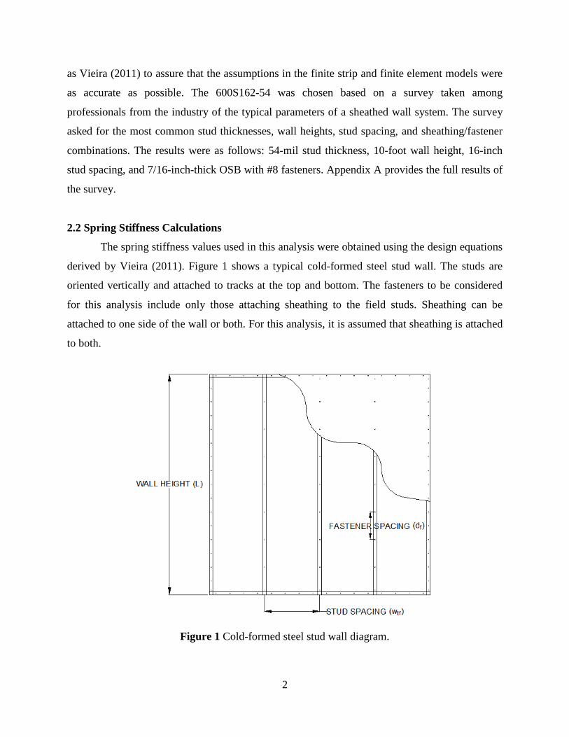
derived by Vieira (2011). Figure 1 shows a typical cold-formed steel stud wall. The studs are
oriented vertically and attached to tracks at the top and bottom. The fasteners to be considered
for this analysis include only those attaching sheathing to the field studs. Sheathing can be
attached to one side of the wall or both. For this analysis, it is assumed that sheathing is attached
to both.
Figure 1 Cold-formed steel stud wall diagram.
2
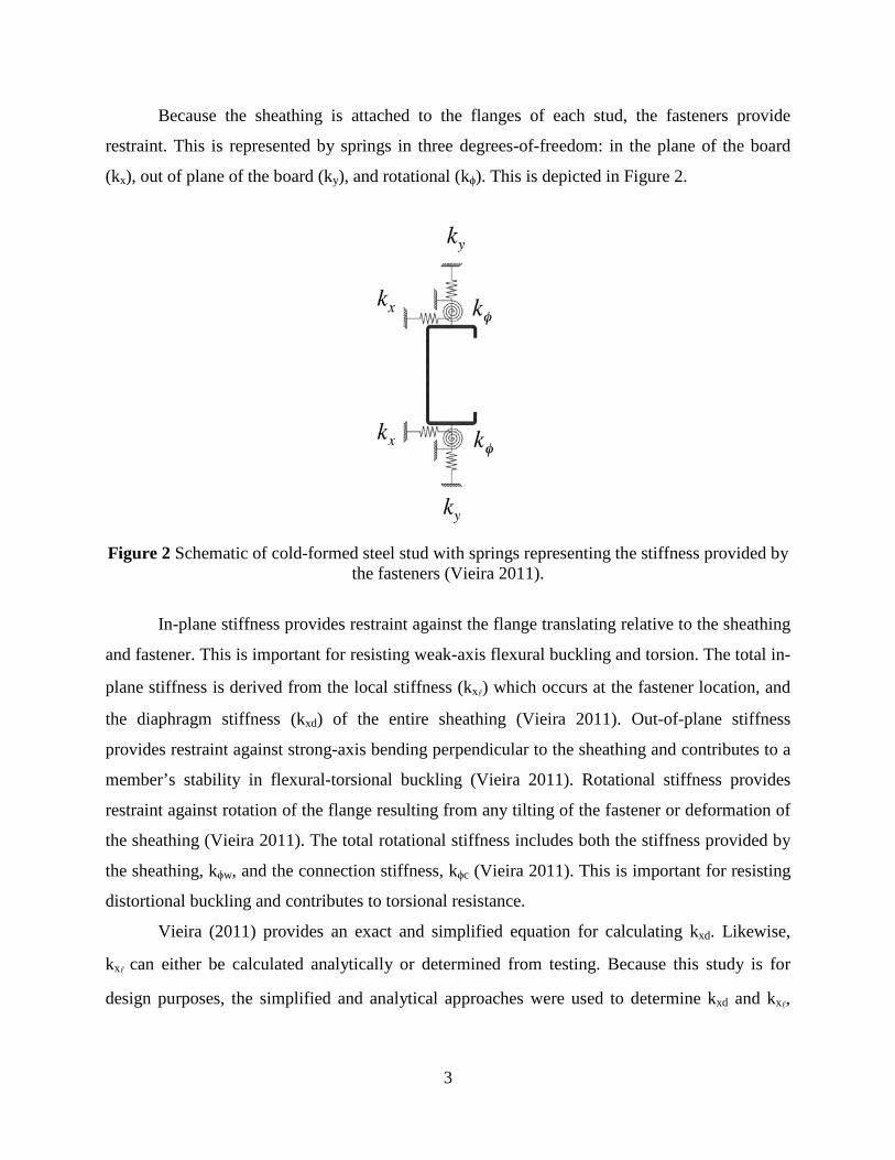
Because the sheathing is attached to the flanges of each stud, the fasteners provide
restraint. This is represented by springs in three degrees-of-freedom: in the plane of the board
(kx), out of plane of the board (ky), and rotational (kϕ). This is depicted in Figure 2.
Figure 2 Schematic of cold-formed steel stud with springs representing the stiffness provided by
the fasteners (Vieira 2011).
In-plane stiffness provides restraint against the flange translating relative to the sheathing
and fastener. This is important for resisting weak-axis flexural buckling and torsion. The total in-
plane stiffness is derived from the local stiffness (kx) which occurs at the fastener location, and
the diaphragm stiffness (kxd) of the entire sheathing (Vieira 2011). Out-of-plane stiffness
provides restraint against strong-axis bending perpendicular to the sheathing and contributes to a
member’s stability in flexural-torsional buckling (Vieira 2011). Rotational stiffness provides
restraint against rotation of the flange resulting from any tilting of the fastener or deformation of
the sheathing (Vieira 2011). The total rotational stiffness includes both the stiffness provided by
the sheathing, kϕw, and the connection stiffness, kϕc (Vieira 2011). This is important for resisting
distortional buckling and contributes to torsional resistance.
Vieira (2011) provides an exact and simplified equation for calculating kxd. Likewise,
kx can either be calculated analytically or determined from testing. Because this study is for
design purposes, the simplified and analytical approaches were used to determine kxd and kx,
3
respectively. Also, kϕ can be determined from tests, but the semi-empirical equations from Vieira
(2011) were used.
The simplified equation for kxd and the analytical equation for kx are as follows:
2
2
LwdGt
k tffboardxd
π= (1)
where:
G = shear stiffness of the sheathing (ksi)
tboard = thickness of the sheathing (in)
df = fastener spacing (in)
wtf = stud spacing/tributary width of fastener (in)
L = height of sheathing/length of member (in)
Likewise, the equation for kx is:
)169(4
3342
34
ttdttEdk
boardboardx +=
ππ
(2)
where:
E = Young’s modulus for cold-formed steel (ksi)
d = diameter of fastener (in)
t = stud thickness (in)
tboard = thickness of sheathing (in)
From the local and diaphragm stiffness values, the overall in-plane stiffness for discrete and
smeared conditions, respectively, is calculated as follows: 1
11−
+=
xdxx kk
k
(3)
f
xx d
kk = (4)
The out-of-plane stiffness ky is calculated from:
4
4)(L
dEIk fparallelw
y
π−= (5)
f
yy d
kk = (6)
4
where:
(EI)w-parallel = sheathing rigidity based on the stress parallel to the strength axis (k-in2/ft)
df = fastener spacing (in)
L = height of sheathing/length of member (in)
The equations for rotational stiffness are as follows:
75000035.0 2 += Etk cφ (7)
f
larperpendicuww d
EIk −=
)(φ (8)
+
=
wc kk
k
φφ
φ11
1 (9)
fdkk φφ = (10)
where:
E = Young’s modulus for cold-formed steel (psi)
t = stud thickness (in)
(EI)w-perpendicular = sheathing rigidity based on the stress perpendicular to the strength axis
(lb-in2/in)
df = fastener spacing (in)
It should be noted that in equation (7), E is in units of psi and t is in units of inches. In
equation (8), (EI)w-perpendicular is in units of lb∙in2/in. Equation (9) gives the rotational stiffness in
units of kips∙in/in/rad. This is the smeared stiffness that must be applied to springs in CUFSM.
To obtain the stiffness for discrete springs, the result is multiplied by df to give the stiffness in
units of kips∙in/rad (equation 10). However, equations (3) and (5) give kx and ky in units of
kips/in. These values must be divided by df to give the values for smeared springs, kx and ky, in
units of kips/in/in. This is expressed in equations (4) and (6), respectively.
3.0 ANALYSIS of 362S162-68
Vieira (2011) provides a thorough design example using CUFSM with spring stiffness
values calculated from the equations. An example is also provided in Appendix B of this report.
The parameters include a 96-inch-long 362S162-68 section, 7/16-inch-thick OSB sheathing, and
#8 fasteners spaced at 12 inches along the length of the member with tributary width (stud
5
spacing) of 24 inches. The procedure for analyzing the member in CUFSM provided by Vieira
(2011) was closely followed, with the exception of the use of the constrained finite strip method
(cFSM), which was not used for analyzing members with fixed boundary conditions in this
study.
3.1 CUFSM Models
The first step was to create a CUFSM model of a 96-inch-long 362S162-68 section. The
latest version of CUFSM (version 4.03) was used, which allows for the implementation of
general boundary conditions in addition to the traditional signature curve analysis. It should be
noted that all models used out-to-out dimensions rather than centerline dimensions. In addition,
rounded corners were neglected. All geometric dimensions for the section were obtained from
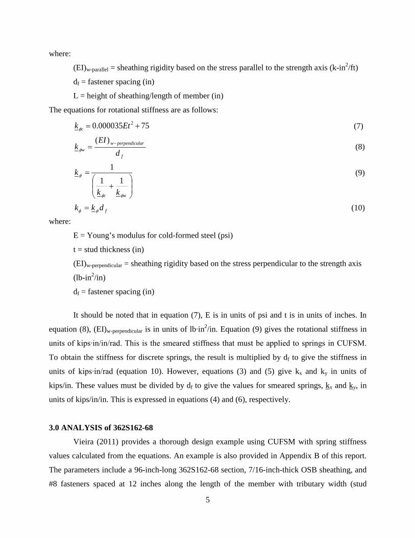
the AISI Cold-Formed Steel Design Manual. Both the actual dimensions and simplified model
dimensions are illustrated in Figure 3. The cross-sectional area of the member is 0.524 in2 and
the design thickness is 0.0713 in.
(a) (b)
Figure 3 (a) Actual dimensions and (b) simplified dimensions of 362S162-68 section.
3.1.1 Signature Curve (Simply-Supported Boundary Conditions)
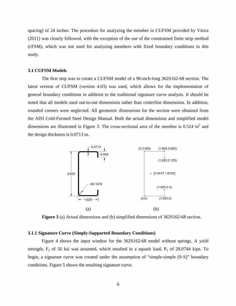
Figure 4 shows the input window for the 362S162-68 model without springs. A yield
strength, Fy of 50 ksi was assumed, which resulted in a squash load, Py of 28.0744 kips. To
begin, a signature curve was created under the assumption of “simple-simple (S-S)” boundary
conditions. Figure 5 shows the resulting signature curve.
6
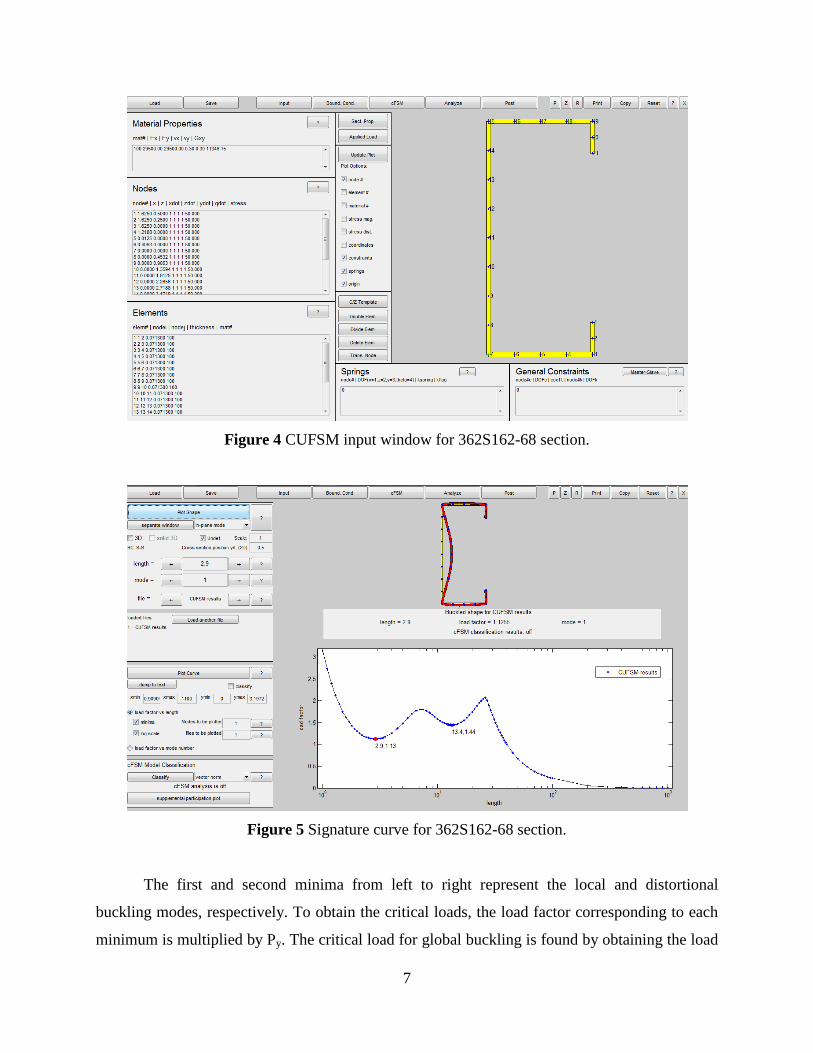
Figure 4 CUFSM input window for 362S162-68 section.
Figure 5 Signature curve for 362S162-68 section.
The first and second minima from left to right represent the local and distortional
buckling modes, respectively. To obtain the critical loads, the load factor corresponding to each
minimum is multiplied by Py. The critical load for global buckling is found by obtaining the load
7
factor corresponding to the length of the member, which in this case is 96 inches, and
multiplying that by Py.
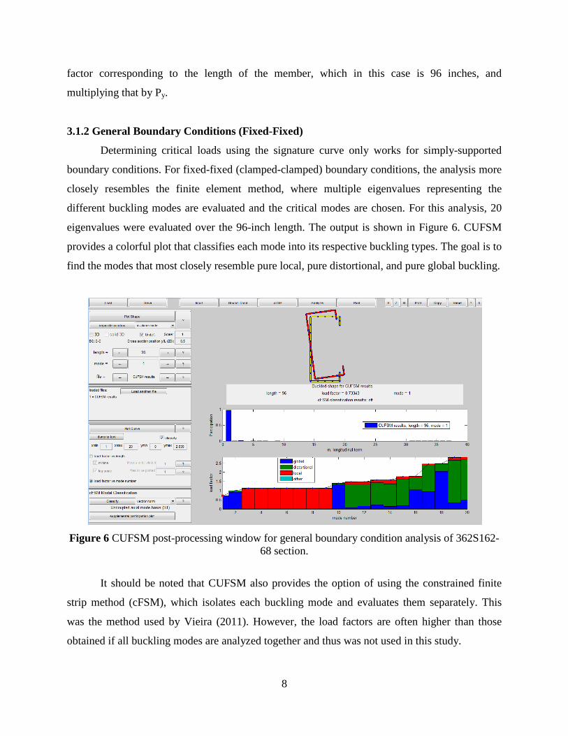
3.1.2 General Boundary Conditions (Fixed-Fixed)
Determining critical loads using the signature curve only works for simply-supported
boundary conditions. For fixed-fixed (clamped-clamped) boundary conditions, the analysis more
closely resembles the finite element method, where multiple eigenvalues representing the
different buckling modes are evaluated and the critical modes are chosen. For this analysis, 20
eigenvalues were evaluated over the 96-inch length. The output is shown in Figure 6. CUFSM
provides a colorful plot that classifies each mode into its respective buckling types. The goal is to
find the modes that most closely resemble pure local, pure distortional, and pure global buckling.
Figure 6 CUFSM post-processing window for general boundary condition analysis of 362S162-
68 section.
It should be noted that CUFSM also provides the option of using the constrained finite
strip method (cFSM), which isolates each buckling mode and evaluates them separately. This
was the method used by Vieira (2011). However, the load factors are often higher than those
obtained if all buckling modes are analyzed together and thus was not used in this study.
8
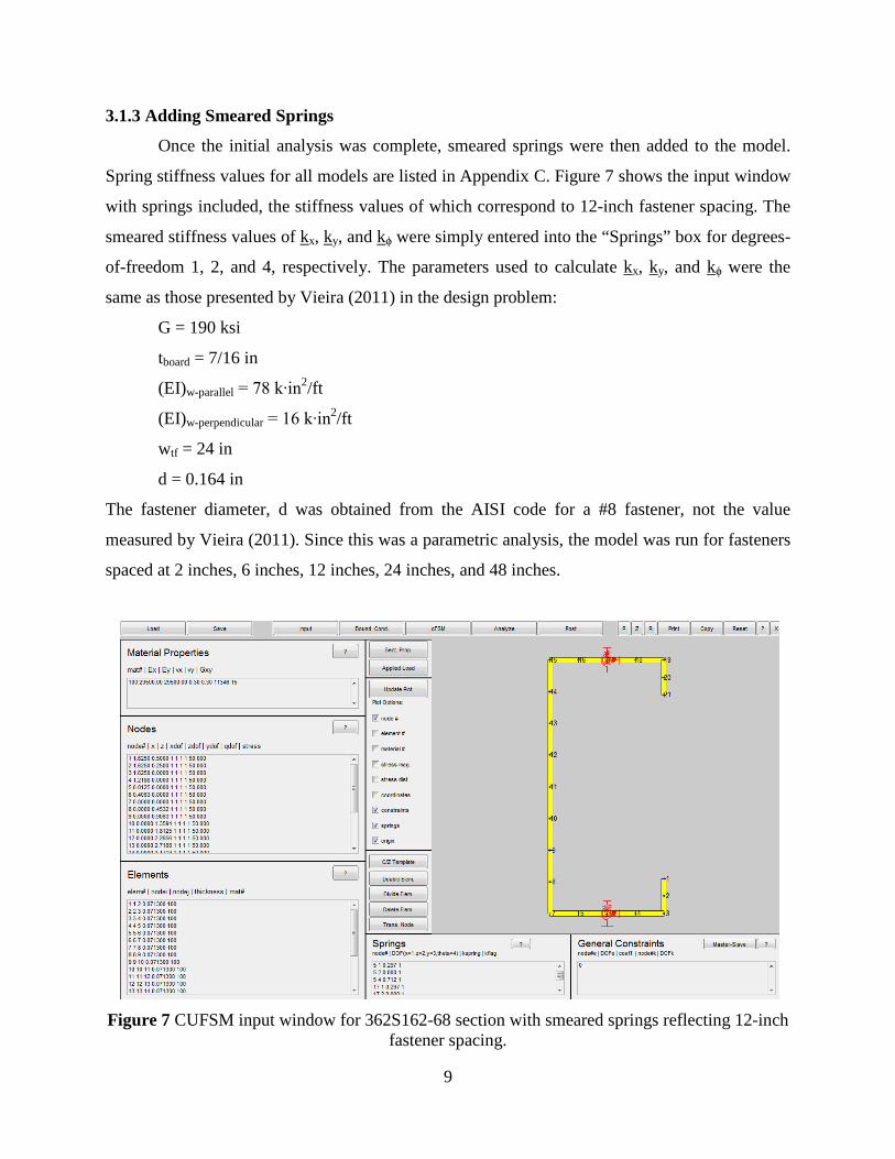
3.1.3 Adding Smeared Springs
Once the initial analysis was complete, smeared springs were then added to the model.
Spring stiffness values for all models are listed in Appendix C. Figure 7 shows the input window
with springs included, the stiffness values of which correspond to 12-inch fastener spacing. The
smeared stiffness values of kx, ky, and kϕ were simply entered into the “Springs” box for degrees-
of-freedom 1, 2, and 4, respectively. The parameters used to calculate kx, ky, and kϕ were the
same as those presented by Vieira (2011) in the design problem:
G = 190 ksi
tboard = 7/16 in
(EI)w-parallel = 78 k∙in2/ft
(EI)w-perpendicular = 16 k∙in2/ft
wtf = 24 in
d = 0.164 in
The fastener diameter, d was obtained from the AISI code for a #8 fastener, not the value
measured by Vieira (2011). Since this was a parametric analysis, the model was run for fasteners
spaced at 2 inches, 6 inches, 12 inches, 24 inches, and 48 inches.
Figure 7 CUFSM input window for 362S162-68 section with smeared springs reflecting 12-inch
fastener spacing.
9
3.2 ABAQUS Models
The other half of this study involved creating finite element models of the member in
ABAQUS. A buckling analysis of the shell element model was performed and the local,
distortional, and global modes were found from the eigenvalues evaluated. ABAQUS CAE was
used for this study, although the input file could also be used to directly create the models.
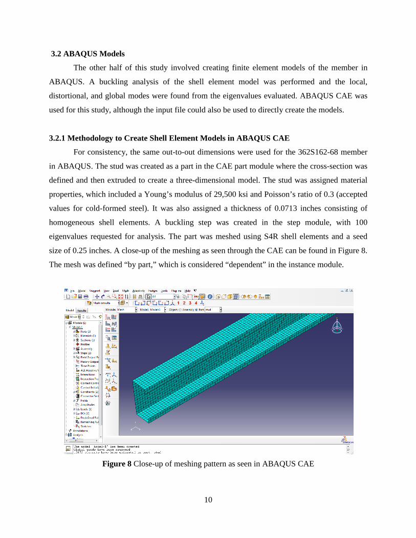
3.2.1 Methodology to Create Shell Element Models in ABAQUS CAE
For consistency, the same out-to-out dimensions were used for the 362S162-68 member
in ABAQUS. The stud was created as a part in the CAE part module where the cross-section was
defined and then extruded to create a three-dimensional model. The stud was assigned material
properties, which included a Young’s modulus of 29,500 ksi and Poisson’s ratio of 0.3 (accepted
values for cold-formed steel). It was also assigned a thickness of 0.0713 inches consisting of
homogeneous shell elements. A buckling step was created in the step module, with 100
eigenvalues requested for analysis. The part was meshed using S4R shell elements and a seed
size of 0.25 inches. A close-up of the meshing as seen through the CAE can be found in Figure 8.
The mesh was defined “by part,” which is considered “dependent” in the instance module.
Figure 8 Close-up of meshing pattern as seen in ABAQUS CAE
10
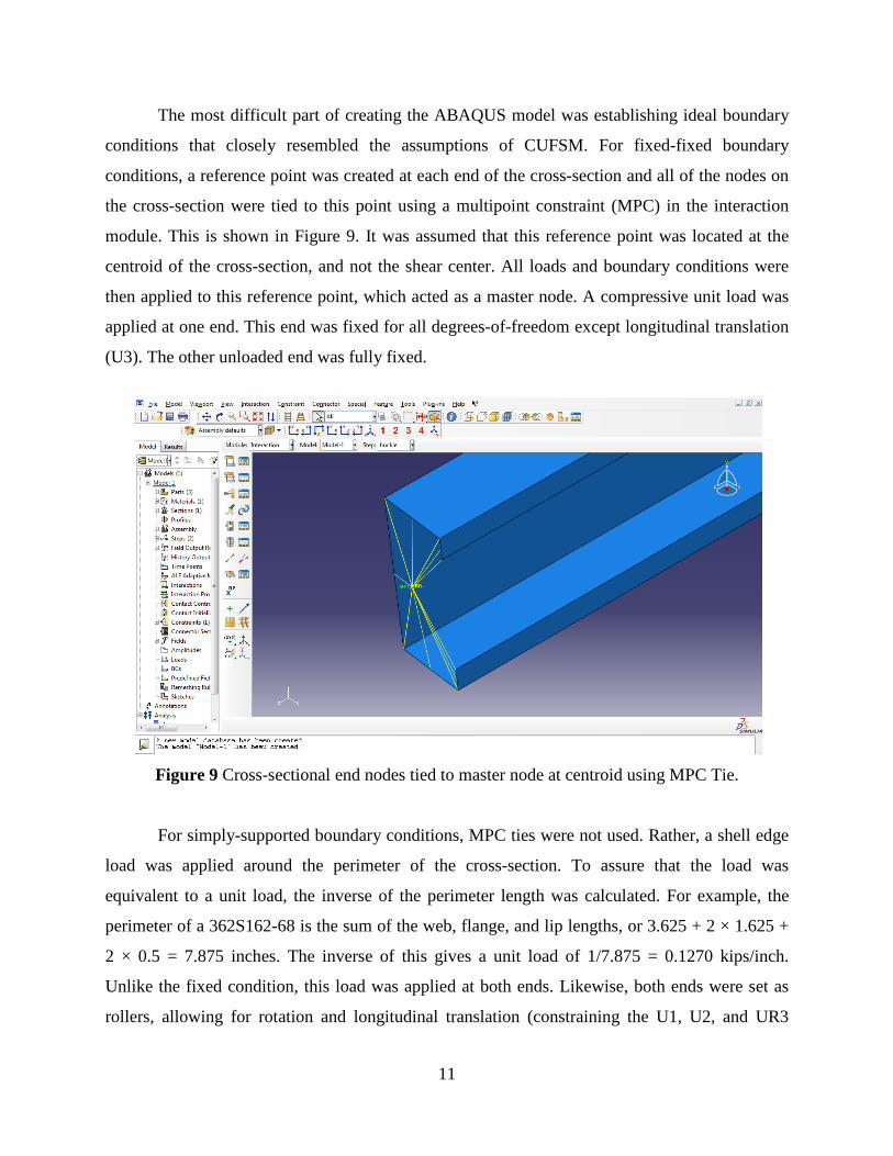
The most difficult part of creating the ABAQUS model was establishing ideal boundary
conditions that closely resembled the assumptions of CUFSM. For fixed-fixed boundary
conditions, a reference point was created at each end of the cross-section and all of the nodes on
the cross-section were tied to this point using a multipoint constraint (MPC) in the interaction
module. This is shown in Figure 9. It was assumed that this reference point was located at the
centroid of the cross-section, and not the shear center. All loads and boundary conditions were
then applied to this reference point, which acted as a master node. A compressive unit load was
applied at one end. This end was fixed for all degrees-of-freedom except longitudinal translation
(U3). The other unloaded end was fully fixed.
Figure 9 Cross-sectional end nodes tied to master node at centroid using MPC Tie.
For simply-supported boundary conditions, MPC ties were not used. Rather, a shell edge
load was applied around the perimeter of the cross-section. To assure that the load was
equivalent to a unit load, the inverse of the perimeter length was calculated. For example, the
perimeter of a 362S162-68 is the sum of the web, flange, and lip lengths, or 3.625 + 2 × 1.625 +
2 × 0.5 = 7.875 inches. The inverse of this gives a unit load of 1/7.875 = 0.1270 kips/inch.
Unlike the fixed condition, this load was applied at both ends. Likewise, both ends were set as
rollers, allowing for rotation and longitudinal translation (constraining the U1, U2, and UR3
11
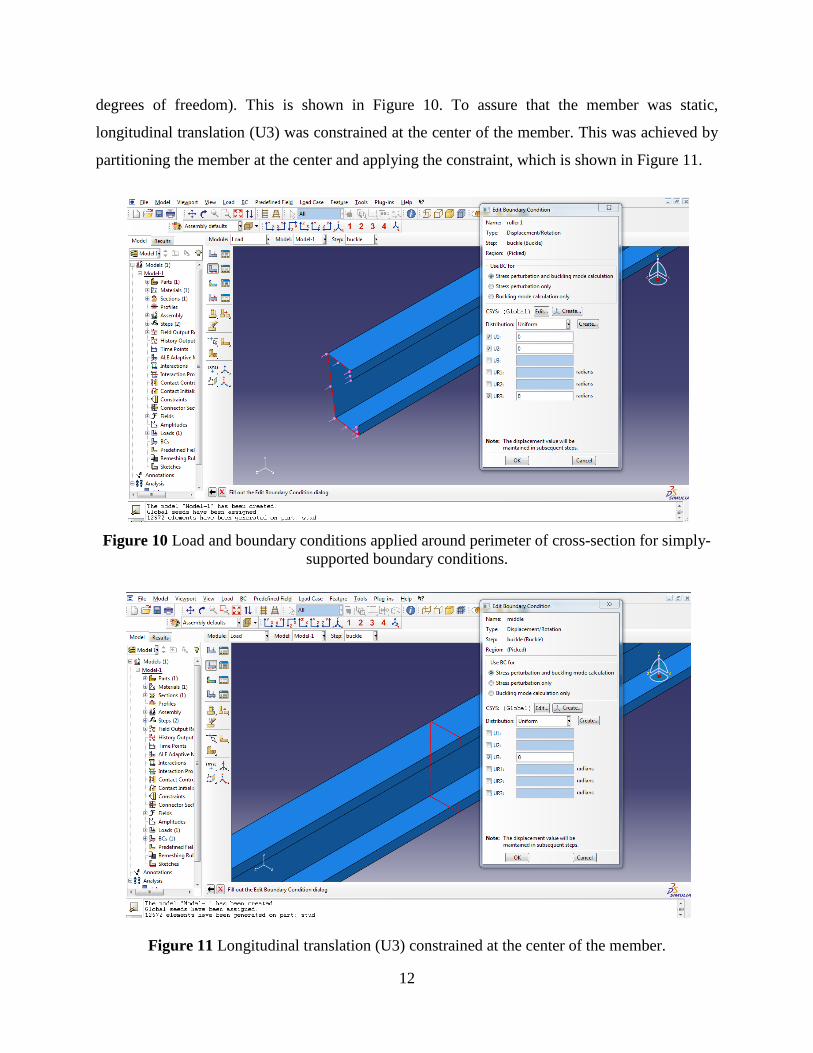
degrees of freedom). This is shown in Figure 10. To assure that the member was static,
longitudinal translation (U3) was constrained at the center of the member. This was achieved by
partitioning the member at the center and applying the constraint, which is shown in Figure 11.
Figure 10 Load and boundary conditions applied around perimeter of cross-section for simply-
supported boundary conditions.
Figure 11 Longitudinal translation (U3) constrained at the center of the member.
12
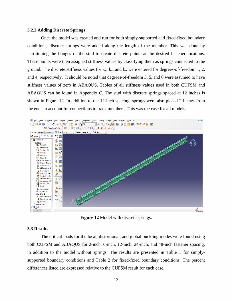
3.2.2 Adding Discrete Springs
Once the model was created and run for both simply-supported and fixed-fixed boundary
conditions, discrete springs were added along the length of the member. This was done by
partitioning the flanges of the stud to create discrete points at the desired fastener locations.
These points were then assigned stiffness values by classifying them as springs connected to the
ground. The discrete stiffness values for kx, ky, and kϕ were entered for degrees-of-freedom 1, 2,
and 4, respectively. It should be noted that degrees-of-freedom 3, 5, and 6 were assumed to have
stiffness values of zero in ABAQUS. Tables of all stiffness values used in both CUFSM and
ABAQUS can be found in Appendix C. The stud with discrete springs spaced at 12 inches is
shown in Figure 12. In addition to the 12-inch spacing, springs were also placed 2 inches from
the ends to account for connections to track members. This was the case for all models.
Figure 12 Model with discrete springs.
3.3 Results
The critical loads for the local, distortional, and global buckling modes were found using
both CUFSM and ABAQUS for 2-inch, 6-inch, 12-inch, 24-inch, and 48-inch fastener spacing,
in addition to the model without springs. The results are presented in Table 1 for simply-
supported boundary conditions and Table 2 for fixed-fixed boundary conditions. The percent
differences listed are expressed relative to the CUFSM result for each case.
13
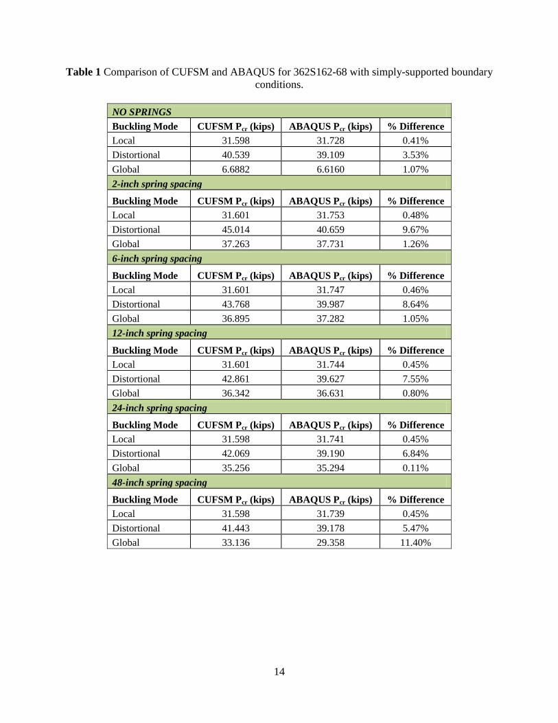
Table 1 Comparison of CUFSM and ABAQUS for 362S162-68 with simply-supported boundary conditions.
NO SPRINGS Buckling Mode CUFSM Pcr (kips) ABAQUS Pcr (kips) % Difference Local 31.598 31.728 0.41% Distortional 40.539 39.109 3.53% Global 6.6882 6.6160 1.07% 2-inch spring spacing
Buckling Mode CUFSM Pcr (kips) ABAQUS Pcr (kips) % Difference Local 31.601 31.753 0.48% Distortional 45.014 40.659 9.67% Global 37.263 37.731 1.26% 6-inch spring spacing
Buckling Mode CUFSM Pcr (kips) ABAQUS Pcr (kips) % Difference Local 31.601 31.747 0.46% Distortional 43.768 39.987 8.64% Global 36.895 37.282 1.05% 12-inch spring spacing
Buckling Mode CUFSM Pcr (kips) ABAQUS Pcr (kips) % Difference Local 31.601 31.744 0.45% Distortional 42.861 39.627 7.55% Global 36.342 36.631 0.80% 24-inch spring spacing
Buckling Mode CUFSM Pcr (kips) ABAQUS Pcr (kips) % Difference Local 31.598 31.741 0.45% Distortional 42.069 39.190 6.84% Global 35.256 35.294 0.11% 48-inch spring spacing
Buckling Mode CUFSM Pcr (kips) ABAQUS Pcr (kips) % Difference Local 31.598 31.739 0.45% Distortional 41.443 39.178 5.47% Global 33.136 29.358 11.40%
14
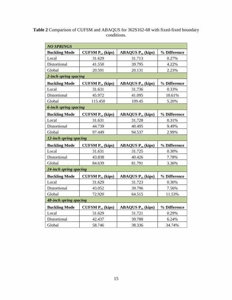
Table 2 Comparison of CUFSM and ABAQUS for 362S162-68 with fixed-fixed boundary conditions.
NO SPRINGS Buckling Mode CUFSM Pcr (kips) ABAQUS Pcr (kips) % Difference Local 31.629 31.713 0.27% Distortional 41.550 39.795 4.22% Global 20.591 20.131 2.23% 2-inch spring spacing
Buckling Mode CUFSM Pcr (kips) ABAQUS Pcr (kips) % Difference Local 31.631 31.736 0.33% Distortional 45.972 41.095 10.61% Global 115.450 109.45 5.20% 6-inch spring spacing
Buckling Mode CUFSM Pcr (kips) ABAQUS Pcr (kips) % Difference Local 31.631 31.728 0.31% Distortional 44.739 40.495 9.49% Global 97.449 94.537 2.99% 12-inch spring spacing
Buckling Mode CUFSM Pcr (kips) ABAQUS Pcr (kips) % Difference Local 31.631 31.725 0.30% Distortional 43.838 40.426 7.78% Global 84.639 81.791 3.36% 24-inch spring spacing
Buckling Mode CUFSM Pcr (kips) ABAQUS Pcr (kips) % Difference Local 31.629 31.723 0.30% Distortional 43.052 39.796 7.56% Global 72.920 64.515 11.53% 48-inch spring spacing
Buckling Mode CUFSM Pcr (kips) ABAQUS Pcr (kips) % Difference Local 31.629 31.721 0.29% Distortional 42.437 39.788 6.24% Global 58.746 38.336 34.74%
15
It can be seen that springs have a strong influence on global buckling. This is evident
from the significant increase in Pcr from the models with no springs to the models with springs at
2-inch spacing. As expected, the global results appear to diverge as fastener spacing increases,
especially for fixed-fixed boundary conditions. The local values appear to be generally consistent
throughout, which is expected as springs typically do not influence local buckling. Also, springs
appear to have only a minimal influence on distortional buckling.
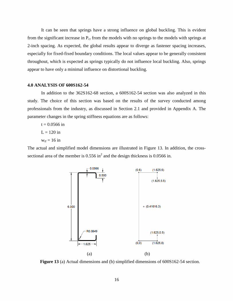
4.0 ANALYSIS OF 600S162-54
In addition to the 362S162-68 section, a 600S162-54 section was also analyzed in this
study. The choice of this section was based on the results of the survey conducted among
professionals from the industry, as discussed in Section 2.1 and provided in Appendix A. The
parameter changes in the spring stiffness equations are as follows:
t = 0.0566 in
L = 120 in
wtf = 16 in
The actual and simplified model dimensions are illustrated in Figure 13. In addition, the cross-
sectional area of the member is 0.556 in2 and the design thickness is 0.0566 in.
(a) (b)
Figure 13 (a) Actual dimensions and (b) simplified dimensions of 600S162-54 section.
16
For this section, 2-inch, 6-inch, 12-inch, 24-inch, 40-inch, and 60-inch fastener spacing
was analyzed. Unlike the 362S162-68 section, which included 48-inch spacing, 40-inch and 60-
inch were chosen for the 600S162-54 since a 120-inch-long stud can be divided into even
increments of 40 inches and 60 inches and not 48 inches. The 60-inch spacing was expected to
have a similar effect on the 120-inch-long 600S162-54 as the 48-inch spacing had on the 96-
inch-long 362S162-68, essentially bisecting it with one fastener in the center and a fastener at
each end.
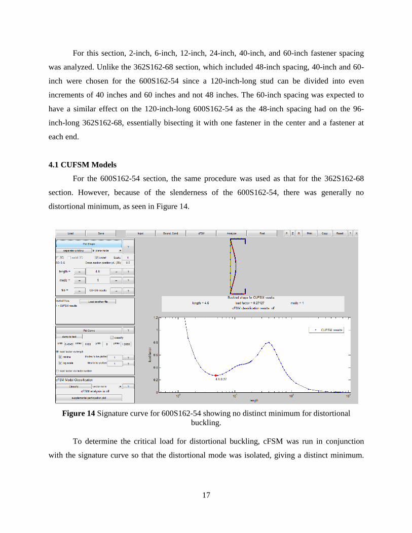
4.1 CUFSM Models
For the 600S162-54 section, the same procedure was used as that for the 362S162-68
section. However, because of the slenderness of the 600S162-54, there was generally no
distortional minimum, as seen in Figure 14.
Figure 14 Signature curve for 600S162-54 showing no distinct minimum for distortional
buckling. To determine the critical load for distortional buckling, cFSM was run in conjunction
with the signature curve so that the distortional mode was isolated, giving a distinct minimum.
17
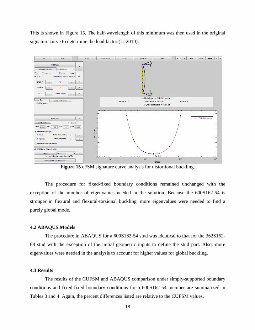
This is shown in Figure 15. The half-wavelength of this minimum was then used in the original
signature curve to determine the load factor (Li 2010).
Figure 15 cFSM signature curve analysis for distortional buckling.
The procedure for fixed-fixed boundary conditions remained unchanged with the
exception of the number of eigenvalues needed in the solution. Because the 600S162-54 is
stronger in flexural and flexural-torsional buckling, more eigenvalues were needed to find a
purely global mode.
4.2 ABAQUS Models
The procedure in ABAQUS for a 600S162-54 stud was identical to that for the 362S162-
68 stud with the exception of the initial geometric inputs to define the stud part. Also, more
eigenvalues were needed in the analysis to account for higher values for global buckling.
4.3 Results
The results of the CUFSM and ABAQUS comparison under simply-supported boundary
conditions and fixed-fixed boundary conditions for a 600S162-54 member are summarized in
Tables 3 and 4. Again, the percent differences listed are relative to the CUFSM values.
18
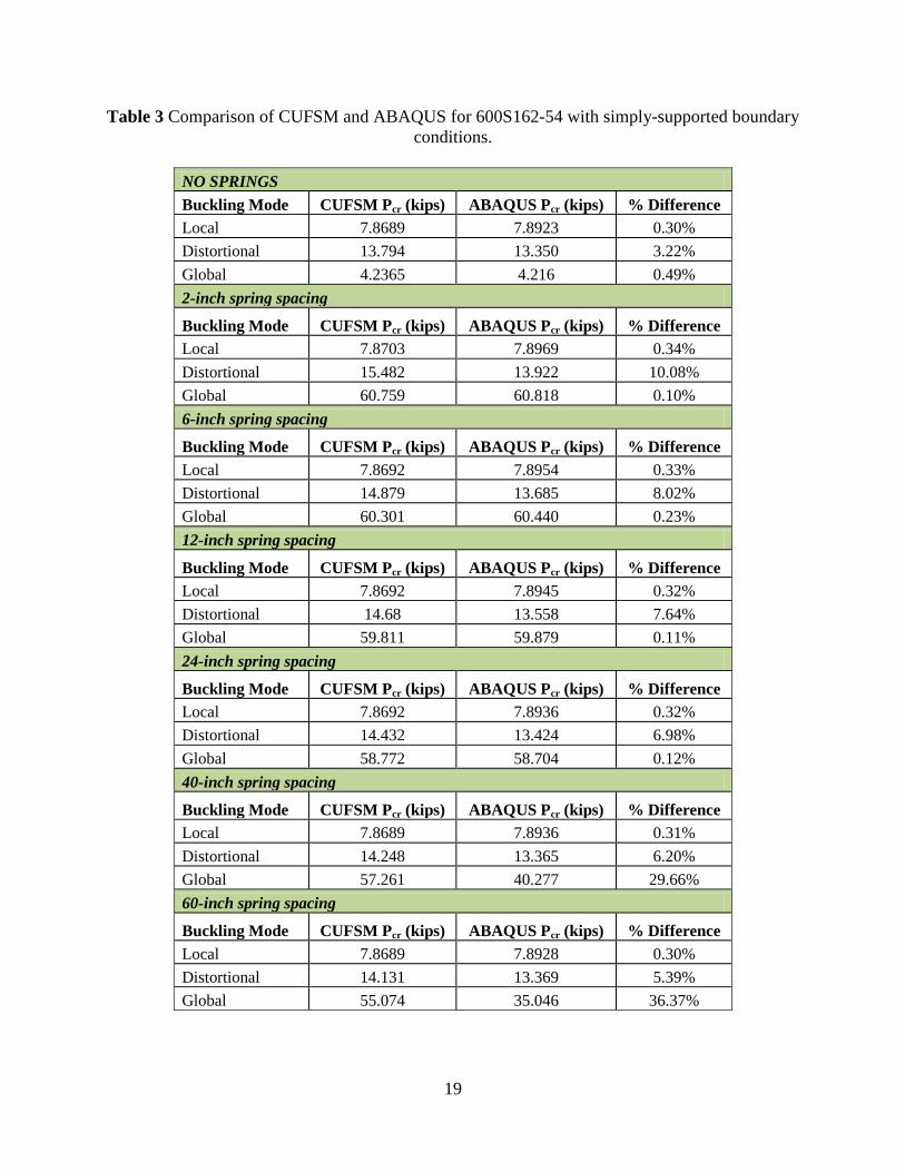
Table 3 Comparison of CUFSM and ABAQUS for 600S162-54 with simply-supported boundary conditions.
NO SPRINGS Buckling Mode CUFSM Pcr (kips) ABAQUS Pcr (kips) % Difference Local 7.8689 7.8923 0.30% Distortional 13.794 13.350 3.22% Global 4.2365 4.216 0.49% 2-inch spring spacing
Buckling Mode CUFSM Pcr (kips) ABAQUS Pcr (kips) % Difference Local 7.8703 7.8969 0.34% Distortional 15.482 13.922 10.08% Global 60.759 60.818 0.10% 6-inch spring spacing
Buckling Mode CUFSM Pcr (kips) ABAQUS Pcr (kips) % Difference Local 7.8692 7.8954 0.33% Distortional 14.879 13.685 8.02% Global 60.301 60.440 0.23% 12-inch spring spacing
Buckling Mode CUFSM Pcr (kips) ABAQUS Pcr (kips) % Difference Local 7.8692 7.8945 0.32% Distortional 14.68 13.558 7.64% Global 59.811 59.879 0.11% 24-inch spring spacing
Buckling Mode CUFSM Pcr (kips) ABAQUS Pcr (kips) % Difference Local 7.8692 7.8936 0.32% Distortional 14.432 13.424 6.98% Global 58.772 58.704 0.12% 40-inch spring spacing
Buckling Mode CUFSM Pcr (kips) ABAQUS Pcr (kips) % Difference Local 7.8689 7.8936 0.31% Distortional 14.248 13.365 6.20% Global 57.261 40.277 29.66% 60-inch spring spacing
Buckling Mode CUFSM Pcr (kips) ABAQUS Pcr (kips) % Difference Local 7.8689 7.8928 0.30% Distortional 14.131 13.369 5.39% Global 55.074 35.046 36.37%
19
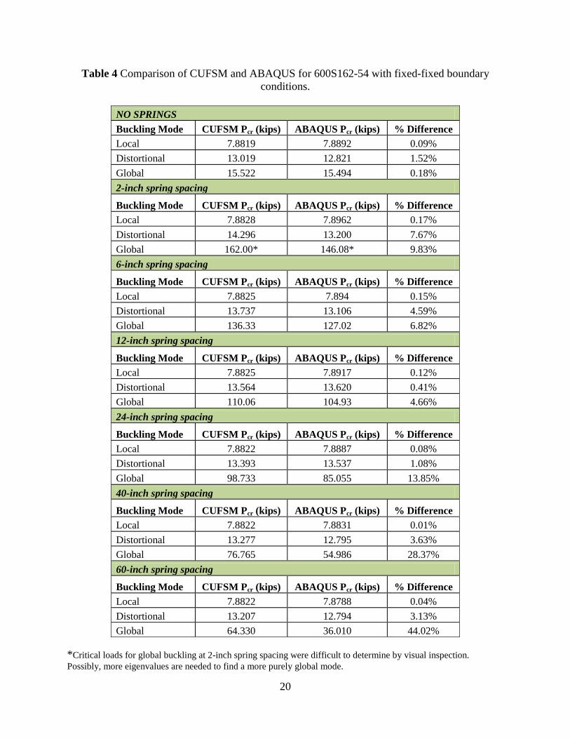
Table 4 Comparison of CUFSM and ABAQUS for 600S162-54 with fixed-fixed boundary conditions.
NO SPRINGS Buckling Mode CUFSM Pcr (kips) ABAQUS Pcr (kips) % Difference Local 7.8819 7.8892 0.09% Distortional 13.019 12.821 1.52% Global 15.522 15.494 0.18% 2-inch spring spacing
Buckling Mode CUFSM Pcr (kips) ABAQUS Pcr (kips) % Difference Local 7.8828 7.8962 0.17% Distortional 14.296 13.200 7.67% Global 162.00* 146.08* 9.83% 6-inch spring spacing
Buckling Mode CUFSM Pcr (kips) ABAQUS Pcr (kips) % Difference Local 7.8825 7.894 0.15% Distortional 13.737 13.106 4.59% Global 136.33 127.02 6.82% 12-inch spring spacing
Buckling Mode CUFSM Pcr (kips) ABAQUS Pcr (kips) % Difference Local 7.8825 7.8917 0.12% Distortional 13.564 13.620 0.41% Global 110.06 104.93 4.66% 24-inch spring spacing
Buckling Mode CUFSM Pcr (kips) ABAQUS Pcr (kips) % Difference Local 7.8822 7.8887 0.08% Distortional 13.393 13.537 1.08% Global 98.733 85.055 13.85% 40-inch spring spacing
Buckling Mode CUFSM Pcr (kips) ABAQUS Pcr (kips) % Difference Local 7.8822 7.8831 0.01% Distortional 13.277 12.795 3.63% Global 76.765 54.986 28.37% 60-inch spring spacing
Buckling Mode CUFSM Pcr (kips) ABAQUS Pcr (kips) % Difference Local 7.8822 7.8788 0.04% Distortional 13.207 12.794 3.13% Global 64.330 36.010 44.02%
*Critical loads for global buckling at 2-inch spring spacing were difficult to determine by visual inspection. Possibly, more eigenvalues are needed to find a more purely global mode.
20
The results for this section show similar patterns to those for the 362S162-68 section. The
critical loads for local buckling show very little variation, regardless of boundary conditions or
fastener spacing. The distortional modes were very difficult to determine by visual inspection in
ABAQUS. Often there were multiple modes that appeared to be distortional with some local
buckling, making it difficult to choose the critical mode. Also, because of the lack of a distinct
distortional minimum on the CUFSM signature curve, the method described provided only an
approximation of the actual critical distortional buckling load.
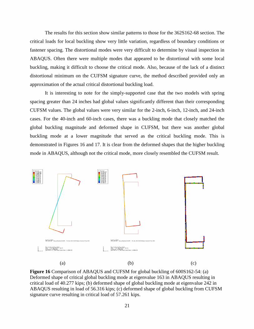
It is interesting to note for the simply-supported case that the two models with spring
spacing greater than 24 inches had global values significantly different than their corresponding
CUFSM values. The global values were very similar for the 2-inch, 6-inch, 12-inch, and 24-inch
cases. For the 40-inch and 60-inch cases, there was a buckling mode that closely matched the
global buckling magnitude and deformed shape in CUFSM, but there was another global
buckling mode at a lower magnitude that served as the critical buckling mode. This is
demonstrated in Figures 16 and 17. It is clear from the deformed shapes that the higher buckling
mode in ABAQUS, although not the critical mode, more closely resembled the CUFSM result.
(a) (b) (c)
Figure 16 Comparison of ABAQUS and CUFSM for global buckling of 600S162-54: (a) Deformed shape of critical global buckling mode at eigenvalue 163 in ABAQUS resulting in critical load of 40.277 kips; (b) deformed shape of global buckling mode at eigenvalue 242 in ABAQUS resulting in load of 56.316 kips; (c) deformed shape of global buckling from CUFSM signature curve resulting in critical load of 57.261 kips.
21
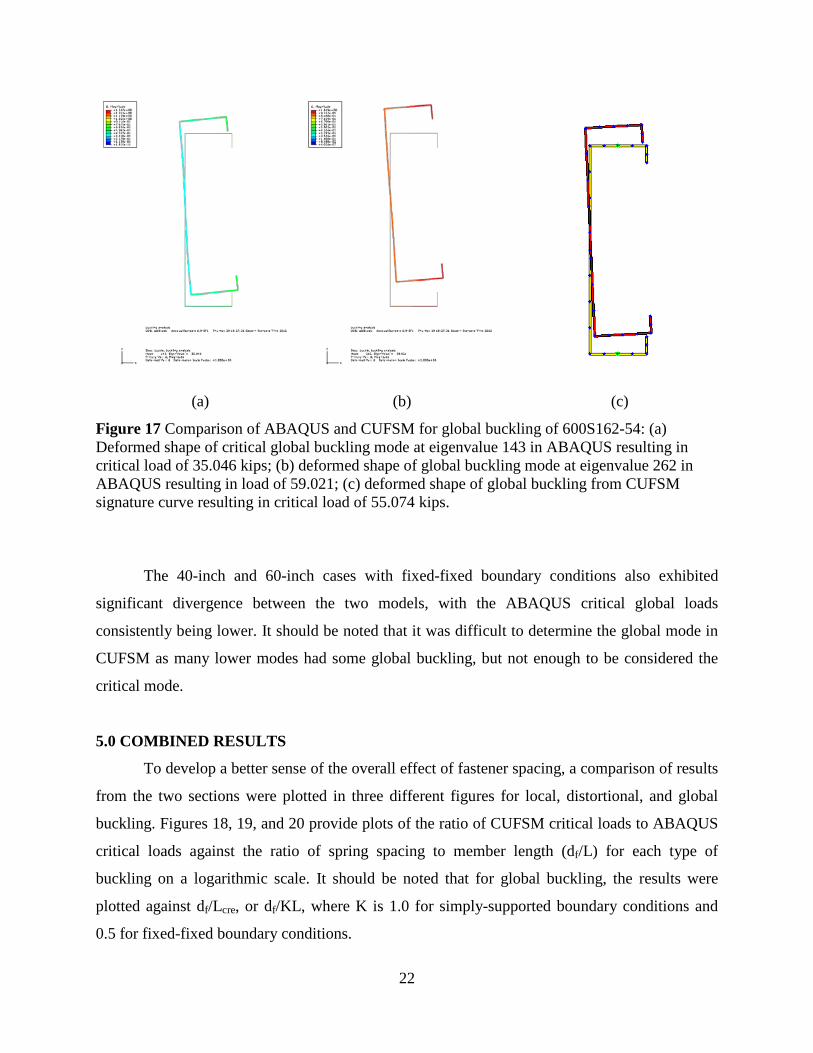
(a) (b) (c)
Figure 17 Comparison of ABAQUS and CUFSM for global buckling of 600S162-54: (a) Deformed shape of critical global buckling mode at eigenvalue 143 in ABAQUS resulting in critical load of 35.046 kips; (b) deformed shape of global buckling mode at eigenvalue 262 in ABAQUS resulting in load of 59.021; (c) deformed shape of global buckling from CUFSM signature curve resulting in critical load of 55.074 kips.
The 40-inch and 60-inch cases with fixed-fixed boundary conditions also exhibited
significant divergence between the two models, with the ABAQUS critical global loads
consistently being lower. It should be noted that it was difficult to determine the global mode in
CUFSM as many lower modes had some global buckling, but not enough to be considered the
critical mode.
5.0 COMBINED RESULTS
To develop a better sense of the overall effect of fastener spacing, a comparison of results
from the two sections were plotted in three different figures for local, distortional, and global
buckling. Figures 18, 19, and 20 provide plots of the ratio of CUFSM critical loads to ABAQUS
critical loads against the ratio of spring spacing to member length (df/L) for each type of
buckling on a logarithmic scale. It should be noted that for global buckling, the results were
plotted against df/Lcre, or df/KL, where K is 1.0 for simply-supported boundary conditions and
0.5 for fixed-fixed boundary conditions.
22
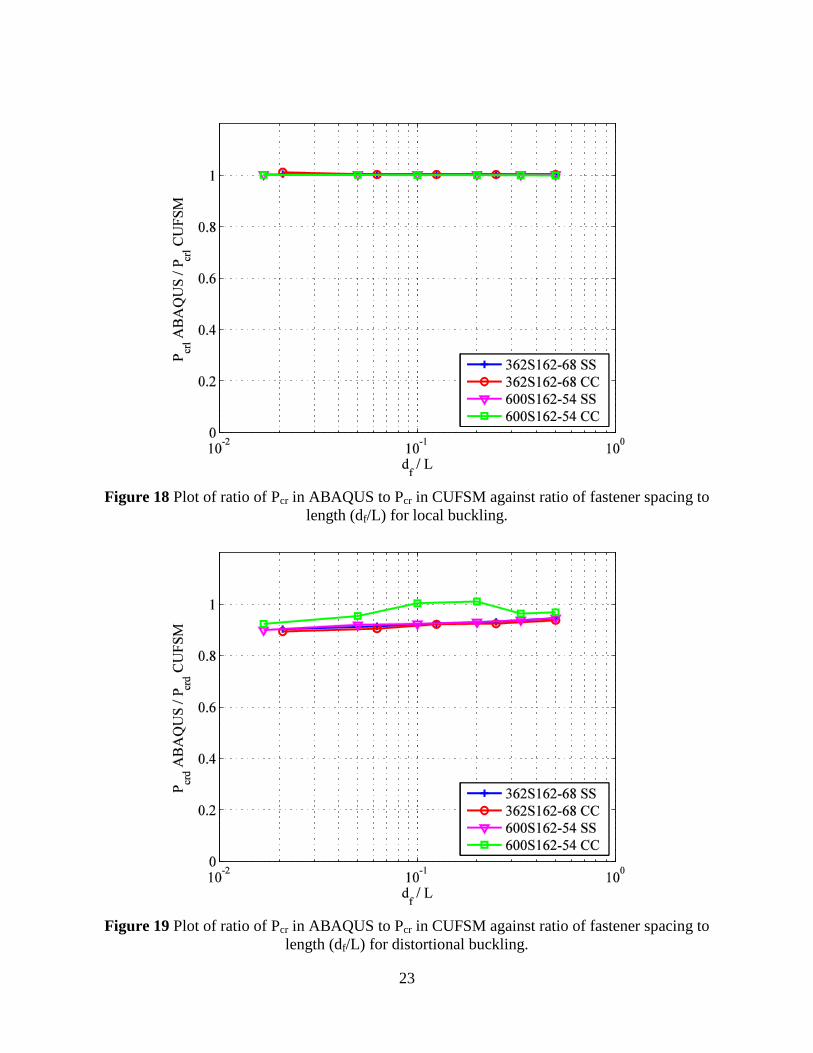
Figure 18 Plot of ratio of Pcr in ABAQUS to Pcr in CUFSM against ratio of fastener spacing to
length (df/L) for local buckling.
Figure 19 Plot of ratio of Pcr in ABAQUS to Pcr in CUFSM against ratio of fastener spacing to
length (df/L) for distortional buckling.
23
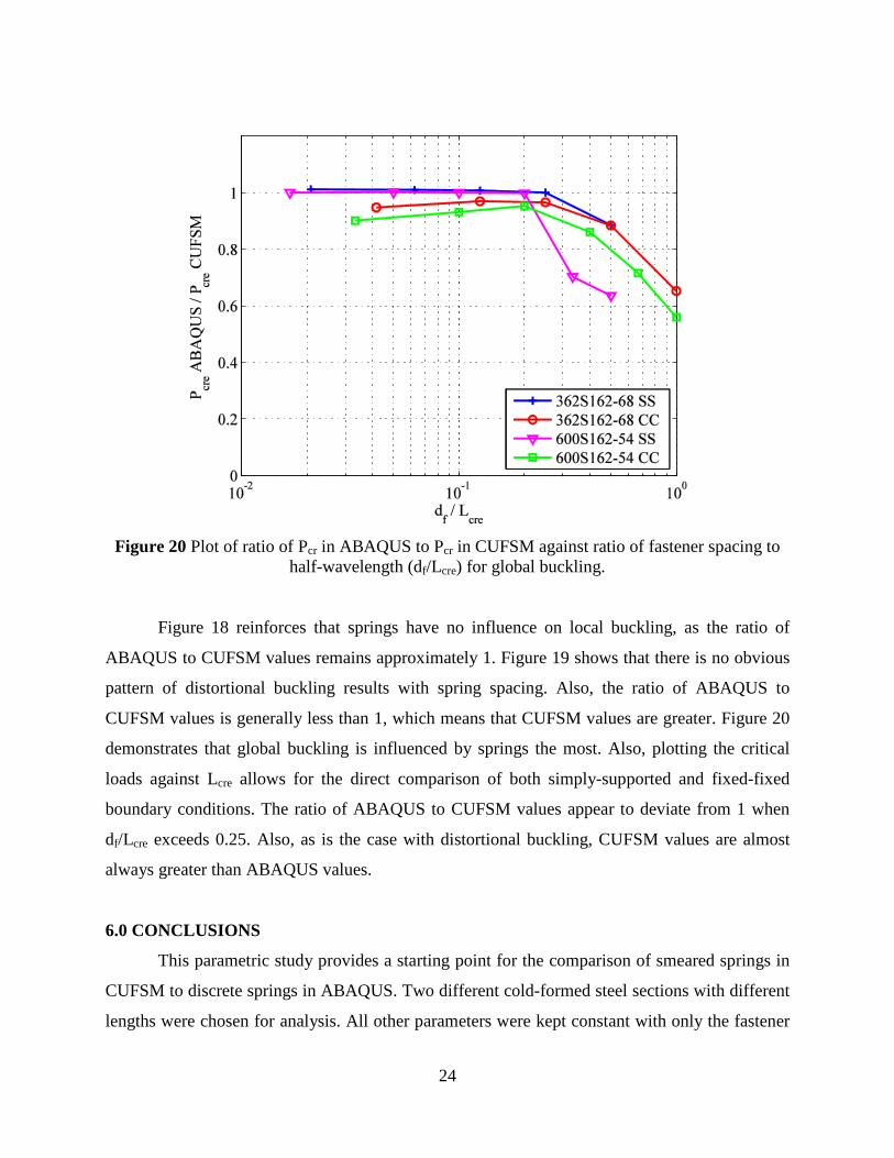
Figure 20 Plot of ratio of Pcr in ABAQUS to Pcr in CUFSM against ratio of fastener spacing to
half-wavelength (df/Lcre) for global buckling. Figure 18 reinforces that springs have no influence on local buckling, as the ratio of
ABAQUS to CUFSM values remains approximately 1. Figure 19 shows that there is no obvious
pattern of distortional buckling results with spring spacing. Also, the ratio of ABAQUS to
CUFSM values is generally less than 1, which means that CUFSM values are greater. Figure 20
demonstrates that global buckling is influenced by springs the most. Also, plotting the critical
loads against Lcre allows for the direct comparison of both simply-supported and fixed-fixed
boundary conditions. The ratio of ABAQUS to CUFSM values appear to deviate from 1 when
df/Lcre exceeds 0.25. Also, as is the case with distortional buckling, CUFSM values are almost
always greater than ABAQUS values.
6.0 CONCLUSIONS
This parametric study provides a starting point for the comparison of smeared springs in
CUFSM to discrete springs in ABAQUS. Two different cold-formed steel sections with different
lengths were chosen for analysis. All other parameters were kept constant with only the fastener
24
spacing varying. The 96-inch 362S162-68 was chosen for direct comparison with Vieira (2011).
The 120-inch 600S162-54, with a deeper cross-section, was chosen to best reflect the most
common parameters selected in a survey. For both cases, it is apparent that spring spacing has no
influence on local buckling and minimal influence on distortional buckling. However, springs
play a significant role in providing restraint against global buckling. Based on the results, it can
be concluded that the smeared spring assumption is only reasonable when df/Lcre ≤ 0.25. Once
that limit is exceeded, the smeared spring assumption should not be used. Also, the fact that
CUFSM results were consistently greater than ABAQUS results means that CUFSM may be
overstating Pcr, which could be problematic if this method is relied upon for design. A further
investigation of boundary condition assumptions should be carried out to assure that both
methods are as accurate as possible. Also, additional members and parameters should be
analyzed to assure that the limit of df/Lcre ≤ 0.25 is consistent.
25
REFERENCES
ABAQUS, ABAQUS/CAE Version 6.9-1, D. Systemes, Editor 2007. AISI, Cold-Formed Steel Design Manual, American Iron and Steel Institute, 2008. AISI-S100, North American Specification for the Design of Cold-Formed Steel Structural Members. American Iron and Steel Institute, 2007. Li, Z., Schafer, B.W. “Application of the finite strip method in cold-formed steel member design.” Journal of Constructional Steel Research, 2010. 66(8-9): p. 971-980. Schafer, B.W., Ádány, S. “Buckling analysis of cold-formed steel members using CUFSM: conventional and constrained finite strip methods. “Eighteenth International Specialty Conference on Cold-Formed Steel Structures, Orlando, FL, October 2006. SSMA, Product Technical Information, ICBO ER-4943P, S.S.M. Associations, Editor 2001. Vieria, L.C.M. (2011). “Behavior and Design of Sheathed Cold-Formed Steel Stud Walls Under Compression,” dissertation, presented to Johns Hopkins University at Baltimore, MD, in fulfillment of the requirements for the degree of Doctor of Philosophy.
26
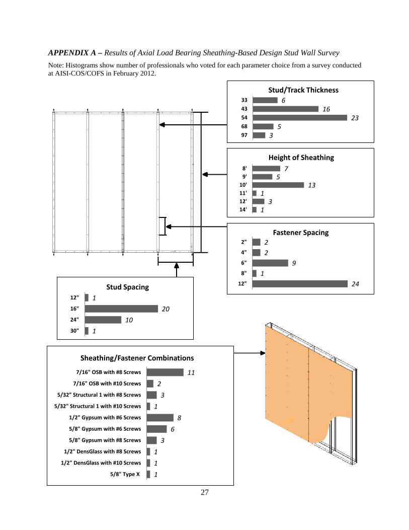
APPENDIX A – Results of Axial Load Bearing Sheathing-Based Design Stud Wall Survey
Note: Histograms show number of professionals who voted for each parameter choice from a survey conducted at AISI-COS/COFS in February 2012.
1
3 1
13 5
7
14' 12' 11' 10'
9' 8'
Height of Sheathing
24
1 9
2 2
12"
8"
6"
4"
2" Fastener Spacing
1
10 20
1
30"
24"
16"
12"
Stud Spacing
1 1 1
3 6
8 1
3 2
11
5/8" Type X
1/2" DensGlass with #10 Screws
1/2" DensGlass with #8 Screws
5/8" Gypsum with #8 Screws
5/8" Gypsum with #6 Screws
1/2" Gypsum with #6 Screws
5/32" Structural 1 with #10 Screws
5/32" Structural 1 with #8 Screws
7/16" OSB with #10 Screws
7/16" OSB with #8 Screws
Sheathing/Fastener Combinations
3
5 23
16 6
97 68 54 43 33
Stud/Track Thickness
27
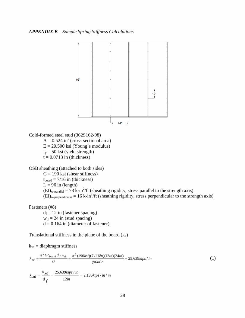
APPENDIX B – Sample Spring Stiffness Calculations
Cold-formed steel stud (362S162-98)
A = 0.524 in2 (cross-sectional area) E = 29,500 ksi (Young’s modulus) fy = 50 ksi (yield strength) t = 0.0713 in (thickness)
OSB sheathing (attached to both sides)
G = 190 ksi (shear stiffness) tboard = 7/16 in (thickness) L = 96 in (length) (EI)w-parallel = 78 k-in2/ft (sheathing rigidity, stress parallel to the strength axis) (EI)w-perpendicular = 16 k-in2/ft (sheathing rigidity, stress perpendicular to the strength axis)
Fasteners (#8) df = 12 in (fastener spacing) wtf = 24 in (stud spacing) d = 0.164 in (diameter of fastener) Translational stiffness in the plane of the board (kx) kxd = diaphragm stiffness
inkipsin
inininksiL
wdGtk tffboard
xd /639.25)96(
)24)(12)(16/7)(190(2
2
2
2
===ππ
(1)
ininkipsin
inkips
fdxdk
xdk //136.212
/639.25===
28
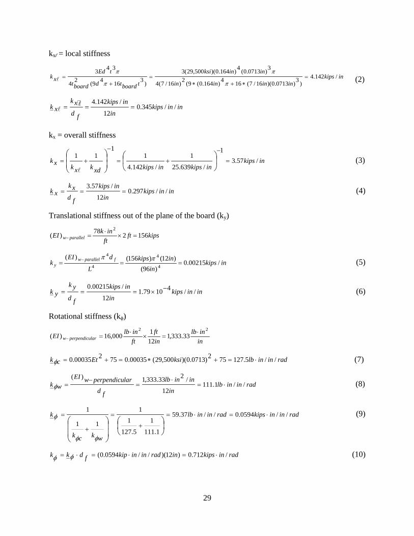
kxl = local stiffness
inkipsinininin
ininksi
tboardtdboardt
tEdxk /142.4
)3)0713.0)(16/7(164)164.0(9(2)16/7(4
3)0713.0(4)164.0)(500,29(3
)31649(24
343=
∗+∗=
+=
π
π
π
π (2)
ininkipsin
inkips
fdxk
xk //345.012
/142.4=== �
kx = overall stiffness
inkipsinkipsinkipsxdkxkxk /57.3
1
/639.25
1
/142.4
11
11=
−
+=
−
+=
(3)
ininkipsin
inkips
fdxk
xk //297.012
/57.3=== (4)
Translational stiffness out of the plane of the board (ky)
kipsftft
inkEI parallelw 156278)(2
=×⋅
=−
inkipsin
inkipsL
dEIk fparallelw
y /00215.0)96(
)12()156()(4
4
4
4
=== − ππ (5)
ininkipsin
inkips
fdyk
yk //41079.112
/00215.0 −×=== (6)
Rotational stiffness (kϕ)
ininlb
inft
ftinlbEI larperpendicuw
2233.333,1
121000,16)( ⋅
=×⋅
=−
radininlbksiEtck //5.127752)0713.0)(500,29(00035.075200035.0 ⋅=+∗=+=φ (7)
radininlbin
ininlb
fdlarperpendicuwEI
wk //1.11112
/233.333,1)(⋅=
⋅=
−=φ (8)
radininkipsradininlb
wkck
k //0594.0//37.59
1.111
1
5.127
1
1
11
1⋅=⋅=
+
=
+
=
φφ
φ (9)
radinkipsinradininkipfdkk /712.0)12)(//0594.0( ⋅=⋅=⋅= φφ (10)
29
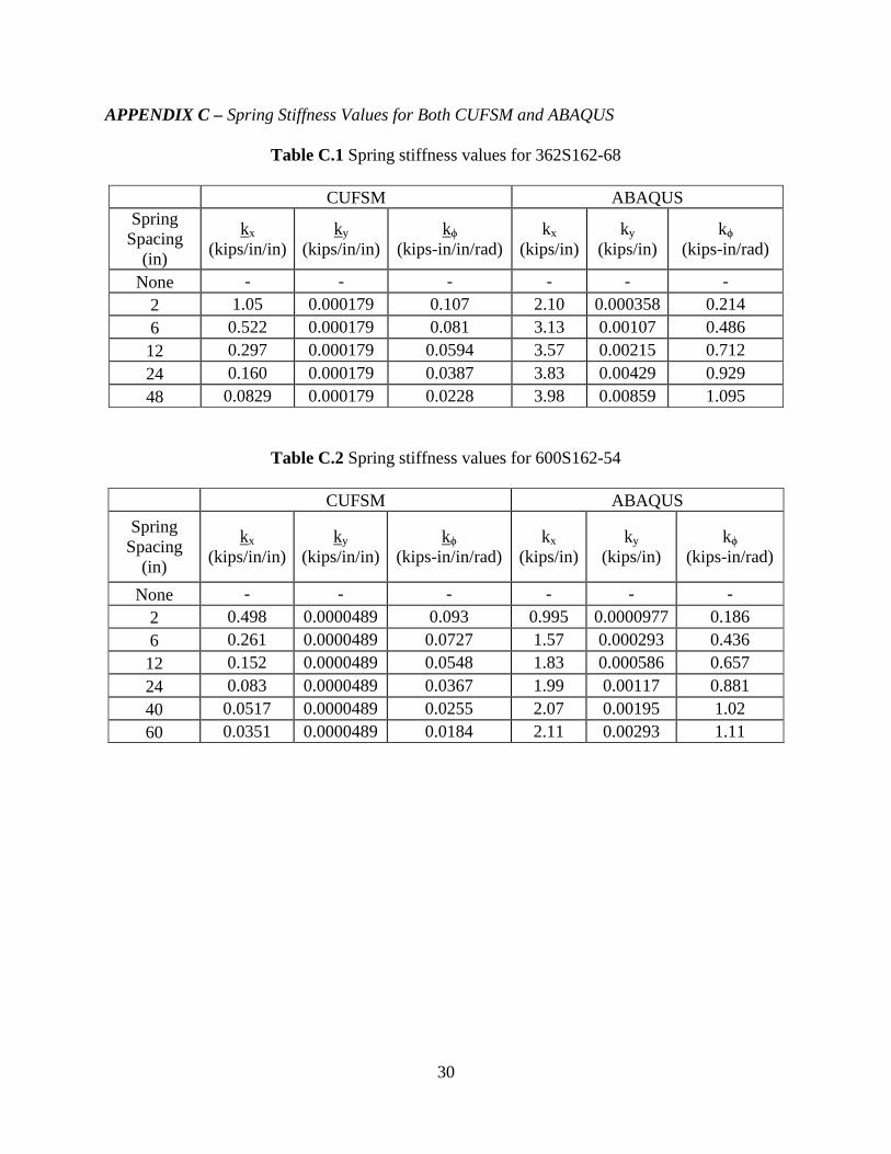
APPENDIX C – Spring Stiffness Values for Both CUFSM and ABAQUS
Table C.1 Spring stiffness values for 362S162-68
CUFSM ABAQUS
Spring Spacing
(in)
kx (kips/in/in)
ky (kips/in/in)
kϕ (kips-in/in/rad)
kx (kips/in)
ky (kips/in)
kϕ (kips-in/rad)
None - - - - - - 2 1.05 0.000179 0.107 2.10 0.000358 0.214 6 0.522 0.000179 0.081 3.13 0.00107 0.486 12 0.297 0.000179 0.0594 3.57 0.00215 0.712 24 0.160 0.000179 0.0387 3.83 0.00429 0.929 48 0.0829 0.000179 0.0228 3.98 0.00859 1.095
Table C.2 Spring stiffness values for 600S162-54
CUFSM ABAQUS
Spring Spacing
(in)
kx (kips/in/in)
ky (kips/in/in)
kϕ (kips-in/in/rad)
kx (kips/in)
ky (kips/in)
kϕ (kips-in/rad)
None - - - - - - 2 0.498 0.0000489 0.093 0.995 0.0000977 0.186 6 0.261 0.0000489 0.0727 1.57 0.000293 0.436 12 0.152 0.0000489 0.0548 1.83 0.000586 0.657 24 0.083 0.0000489 0.0367 1.99 0.00117 0.881 40 0.0517 0.0000489 0.0255 2.07 0.00195 1.02 60 0.0351 0.0000489 0.0184 2.11 0.00293 1.11
30
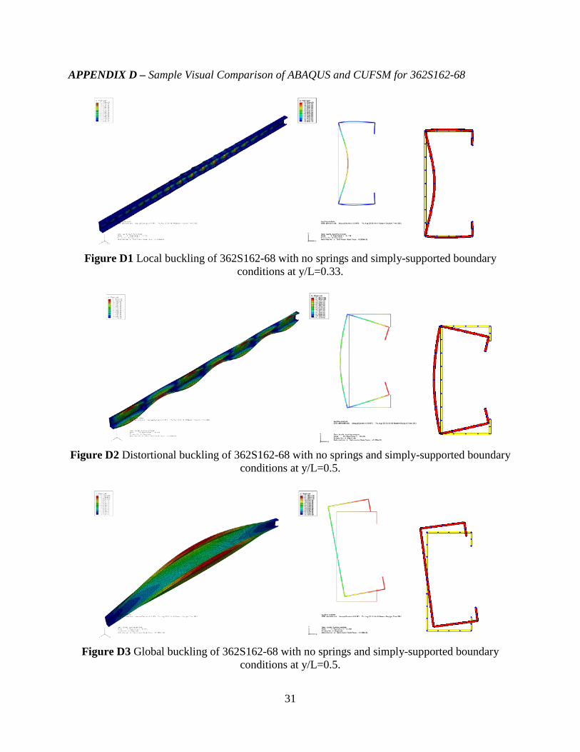
APPENDIX D – Sample Visual Comparison of ABAQUS and CUFSM for 362S162-68
Figure D1 Local buckling of 362S162-68 with no springs and simply-supported boundary
conditions at y/L=0.33.
Figure D2 Distortional buckling of 362S162-68 with no springs and simply-supported boundary
conditions at y/L=0.5.
Figure D3 Global buckling of 362S162-68 with no springs and simply-supported boundary
conditions at y/L=0.5.
31
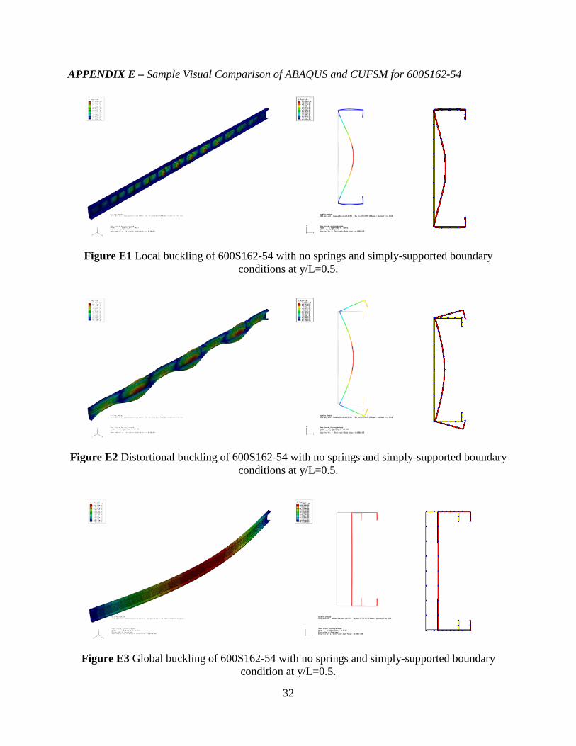
APPENDIX E – Sample Visual Comparison of ABAQUS and CUFSM for 600S162-54
Figure E1 Local buckling of 600S162-54 with no springs and simply-supported boundary
conditions at y/L=0.5.
Figure E2 Distortional buckling of 600S162-54 with no springs and simply-supported boundary
conditions at y/L=0.5.
Figure E3 Global buckling of 600S162-54 with no springs and simply-supported boundary
condition at y/L=0.5.
32