Fast Orthogonal Search For Training Radial BasisFunction Neural NetworksBy Wahid AhmedThesis Advisor: Donald M. Hummels, Ph.D.An Abstract of the Thesis Presented inPartial Ful�llment of the Requirements for theDegree of Master of Science (in Electrical Engineering).August, 1994This thesis presents a fast orthogonalization process to train a Radial BasisFunction (RBF) neural network. The traditional methods for con�guring the RBFweights is to use some matrix inversion or iterative process. These traditionalapproaches are either time consuming or computationally expensive, and may notconverge to a solution. The goal of this thesis is �rst to use a fast orthogonal-ization process to �nd the nodes of the RBF network which produce the mostimprovement on a target function, and then to �nd the weights for these nodes.Three applications of RBF networks using this fast orthogonal search techniqueare presented. The �rst problem involves characterization of an analog-to-digitalconverter (ADC), where the goal is to build an error table to compensate the er-ror generated by the physical conversion process of ADC. The second problem isa simple pattern recognition problem, where the goal is to classify a set of 2 di-mensional and 2-class patterns. The �nal problem involves classi�cation of humanchromosomes, which is a highly complicated 30 dimensional and 24 class problem.Experimental results will be presented to show that the fast orthogonal searchtechnique not only outperforms traditional techniques, but it also uses much lesstime and e�ort.

Fast Orthogonal Search For Training Radial BasisFunction Neural NetworksByWahid AhmedA THESISSubmitted in Partial Ful�llment of therequirement for the Degree ofMaster of Science(in Electrical Engineering)The Graduate SchoolUniversity of MaineAugust, 1994Advisory Committee:Donald M. Hummels, Associate Professor of Electrical and Computer Engi-neeringThesis AdvisorMohamad T. Musavi, Associate Professor of Electrical and Computer Engi-neering,Fred H. Irons, Castle Professor of Electrical and Computer Engineering,Bruce E. Segee, Assistant Professor of Electrical and Computer Engineering.

iiACKNOWLEDGMENTSAbundant thanks are due to those who, in one respect or another, havecontributed to this project.First, I am greatly indebted to my family for their continued support andencouragement. Without them I couldn't make it this far.I especially wish to express my sincere gratitude to my thesis advisor,Dr. Donald M. Hummels for his patience, guidance, encouragement, and time.Without him this thesis would not have been completed. I envy his sincere, en-thusiastic approach.I express my sincere appreciation to Dr. M. T. Musavi. I owe him every-thing I know in neural networks. He gave me the �rst lesson on neural networks,and he has continued to support my neural network research until now. I havelearned a lot just by working with him. I admire his unstoppable desire for im-provement in every aspect. Lots of thanks goes to him.My sincere appreciation goes to Dr. Fred H. Irons for his inspirational dis-cussions, for his help in understanding the analog-to-digital converters, and forproviding constructive criticism for this thesis.I am grateful to Dr. Bruce E. Segee, for his constructive participation inmy advisory committee.I would like to thank everybody I worked with here in the Electrical andComputer Engineering Department. Thanks goes to, Bruce Little�eld for sharinghis expertise with me in networking, Ioannis Papantonopoulos and Richard Cookfor ADC research, and my coworkers this summer Norm Dutil, Jon Larabee forthe greatest working environment and last but not least, Sekhar Puranapanda fora lot of laughs.Finally, I wish to thank all my friends and faculty for making such a warmenvironment during my stay at the University of Maine.

iiiCONTENTSLIST OF FIGURES iv1 Introduction 11.1 Problem Statement : : : : : : : : : : : : : : : : : : : : : : : : : : : 11.2 Review of Previous Work : : : : : : : : : : : : : : : : : : : : : : : : 21.3 Thesis Overview : : : : : : : : : : : : : : : : : : : : : : : : : : : : : 32 Radial Basis Function Neural Network 42.1 RBF structure : : : : : : : : : : : : : : : : : : : : : : : : : : : : : : 42.2 Solving for the Weights : : : : : : : : : : : : : : : : : : : : : : : : : 72.2.1 Gradient Descent Solution : : : : : : : : : : : : : : : : : : : 72.2.2 Cholesky Decomposition : : : : : : : : : : : : : : : : : : : : 82.2.3 Singular Value Decomposition : : : : : : : : : : : : : : : : : 102.2.4 Orthogonal Search : : : : : : : : : : : : : : : : : : : : : : : 123 The Fast Orthogonal Search 153.1 Mathematical Development : : : : : : : : : : : : : : : : : : : : : : 153.2 Fast Orthogonal Search Algorithm : : : : : : : : : : : : : : : : : : 213.3 Computational Evaluations : : : : : : : : : : : : : : : : : : : : : : 244 Applications of the RBF Network 254.1 Analog to Digital Converter Error Compensation : : : : : : : : : : 254.1.1 Problem Description : : : : : : : : : : : : : : : : : : : : : : 254.1.2 Results : : : : : : : : : : : : : : : : : : : : : : : : : : : : : : 284.2 A Simple Pattern Recognition Problem : : : : : : : : : : : : : : : : 374.3 Classi�cation of Chromosome : : : : : : : : : : : : : : : : : : : : : 444.3.1 RBF Network for Chromosome Classi�cation : : : : : : : : : 444.3.2 Results and Analysis : : : : : : : : : : : : : : : : : : : : : : 465 Conclusion 505.1 Summary : : : : : : : : : : : : : : : : : : : : : : : : : : : : : : : : 505.2 Future Work : : : : : : : : : : : : : : : : : : : : : : : : : : : : : : : 51A PROGRAM LISTING 56A.1 Fast Orthogonal Search : : : : : : : : : : : : : : : : : : : : : : : : : 56B Preparation of This Document 62BIOGRAPHY OF THE AUTHOR 63

ivLIST OF FIGURES2.1 Network structure for the Radial Basis Function Neural Network. : 54.1 ADC Compensation Architecture : : : : : : : : : : : : : : : : : : : 264.2 The domain of the error function. : : : : : : : : : : : : : : : : : : 274.3 An error table. : : : : : : : : : : : : : : : : : : : : : : : : : : : : : 294.4 Measure of SFDR. : : : : : : : : : : : : : : : : : : : : : : : : : : : 304.5 SFDR for the uncompensated, compensated by proposed technique,and compensated by singular value decomposition. : : : : : : : : : 324.6 The sum squared error for the network as each node gets added in. 334.7 The selection of 50 nodes out of 500 initial nodes. : : : : : : : : : 344.8 The selection of 50 nodes out of the 4 layered nodes. : : : : : : : : 364.9 The training sample for the 2D 2-class problem. : : : : : : : : : : 384.10 The percentage error vs � for the 2D 2-class problem. : : : : : : : 394.11 The output surface of the RBF for the 2D 2-class problem. : : : : 414.12 The sum squared error of the training samples for the 2D 2-classproblem. : : : : : : : : : : : : : : : : : : : : : : : : : : : : : : : : 424.13 The node selection process of the orthogonal search technique. : : 434.14 Network structure for the RBF Network for Chromosome Classi�-cation. : : : : : : : : : : : : : : : : : : : : : : : : : : : : : : : : : 454.15 The sum squared error for training class 1 of the Chromosome prob-lem. : : : : : : : : : : : : : : : : : : : : : : : : : : : : : : : : : : : 484.16 The percent error of the network for di�erent numbers of the initialnode selection : : : : : : : : : : : : : : : : : : : : : : : : : : : : : 49

1CHAPTER 1Introduction1.1 Problem StatementThe neural network is the most exciting interdisciplinary �eld of this decade.The widespread applications of neural networks not only proves their success butalso illustrates the necessity of �nding the best network to solve a problem. It seemslike the general agreement is that no single network can solve all our problems;we need di�erent networks to solve di�erent problems. Back Propagation (BP)[1], Radial Basis Function (RBF) [2, 3], Probabilistic Neural Network (PNN) [4],Kohonen's Self Organizing Map [5] are namely the few well known neural networks.The growth of neural networks has been heavily in uenced by the RadialBasis Function (RBF) neural networks. The application of the RBF network canbe found in pattern recognition [3, 6, 7], function approximation [2, 8], signal pro-cessing [8, 9], system equalization [11] and more. The consistency and convergenceof the RBF network for the approximation of functions has been proven [10]. Alarge amount of research has been also conducted on the architecture of the RBFnetwork. The two most important parameters of a RBF node, the center and thecovariance matrix, have been examined thoroughly [6, 11, 12]. A major issue han-dled by these researchers is the reduction of the number of nodes. This reductioninvolves clustering of the input samples without any consideration of the targetfunction, or the convergence of the weights. The weights (the most signi�cantcomponent of any neural network) of the RBF network were left untouched bymost of the researchers. This oversight is not ignorance but a con�dence on thetraditional approaches. Like many other things, the traditional approaches justdo not work all the time. For RBF weights, the traditional approaches only workwhen the training samples are well behaved. In real life, the training samples

2are not well behaved causing major problems for �nding the RBF weights. Theissue of this thesis is to �nd a set of most signi�cant nodes and their weights fora given network, using a technique that considers both the structure of the inputparameter space and the target function to which the network will be trained.1.2 Review of Previous WorkThe traditional approach to design an RBF network is to �rst select a set ofnetwork parameters (number of nodes, node centers, node covariances) and then�nd the weights by formulating the network by solving a least squares (LS) formu-lations of the problem. Various techniques may be used to solve the LS problemsincluding Singular Value Decomposition (SVD), Cholesky Decomposition, and theGradient Descent approach. These traditional methods have a variety of problems,which will be discussed later. Orthogonal decomposition techniques may be usedto provide an orthogonal basis set for a LS problem. An orthogonal scheme wasused by Chen et. al. [13] in RBF networks to simultaneously con�gure the struc-ture of the network and the weights. The orthogonal search technique presented byChen is cumbersome, and requires redundant calculations making it non-suitablefor reasonable size networks.A similar fast orthogonal search technique has also been developed by Ko-renberg et. al. [14, 15] for nonlinear system identi�cation. This procedure alsoincludes redundant calculations and was highly customized to the problem of �nd-ing the kernels for a nonlinear system with random inputs. This thesis presentsan e�cient fast orthogonal search eliminating the redundancy of [13, 14]. Theresulting algorithm is directly applicable to RBF networks and a wide variety ofother LS approximation problems.

31.3 Thesis OverviewThis thesis has been organized in �ve chapters. Chapter 2 provides the RBFarchitecture along with some traditional approaches to con�gure the weights. InChapter 3 the mathematical development, and a simple algorithm for the proposedfast orthogonal search technique will be presented. Several applications of theRBF network, using the fast orthogonal search technique, will be used to evaluatethe technique in Chapter 4. Chapter 5 concludes the thesis by providing a briefsummary of this research and suggesting some future research directions.

4CHAPTER 2Radial Basis Function Neural Network2.1 RBF structureThe RBF Neural Network gained its popularity for its simplicity and speed.RBF is a simple feed forward neural network with only one hidden layer, andan output layer. The hidden layer is the backbone of the RBF structure. Thehidden layer consists of a set of neurons or nodes with radial basis functions as theactivation function of the neuron, hence the name Radial Basis Function NeuralNetwork. A Gaussian density function is the most widely used activation function.The output layer is simply a summing unit. This layer adds up all of the weightedoutput of the hidden layer. Figure 2.1 illustrates the RBF network.The following equation gives the output of the RBF networky = f(~x) = NXk=1wk�k(~x); (2:1)where �k(~x) = (2�)�p=2j�kj� 12 e� 12 (~x�~ck)�k�1(~x�~ck)T : (2:2)Above, N is the number of network nodes, p is the dimensionality of the inputspace ~x, and wk, ~ck, and �k represent the weight, center, and the covariance matrixassociated with each node. In the above equation the output of the network is ascalar quantity for simplicity, but the network can have any number of outputs.In supervised learning, where input output pairs (~x; y) are presented to\teach" the network, the objective of training is to con�gure a set of weights, wk,such that the network produces the desired output for the given inputs. In thatcase, we say that the network has learned. So if (~x; y) is an input output pair,where ~x is the input and y is the desired output, then the network should learn the

5

ΣSample

w

w

w

w

yx

Input1

3

n

2

Figure 2.1: Network structure for the Radial Basis Function Neural Network.

6mapping function f , where y = f(~x). The training is done using the M trainingsample pairs (~x1; y1); (~x2; y2); � � � (~xM ; yM). The output vector containing the Moutputs of the network can be written using the following matrix form,~y = �~w; (2:3)where ~y is an M dimensional vector and ~w is the N dimensional weight vector.The above quantities aregiven by~y = � y1 y2 � � � yM �T ;~w = � w1 w2 � � � wN �T ;� = 2666664 �1(~x1) �2(~x1) � � � �N(~x1)... ... ...�1(~xM ) �2(~xM) � � � �N(~xM) 3777775 : (2.4)�i(~xj) is the output of ith node for the jth input vector ~xj. So each column of the� matrix contains the output of a node for all M training samples.The problem of �nding the network weights reduces to �nding the vector~w which makes the network output ~y as close as possible to the vector of desirednetwork outputs ~y = [y1 y2 � � � yM ]T . Generally, ~w is determined by �nding theleast square (LS) solution to �~w = ~y: (2:5)The method for �nding the solution to (2.5) depends in large part on the structureof the network being designed. One popular scheme is to center a node of thenetwork on each of the input training samples (~ck = ~xk; k = 1; 2; � � � ; N). In thiscase the matrix � is square, and the weights are given by ~w = ��1~y provided that� is nonsingular. However, calculation of ��1 is often problematic, particularlyfor large networks.

7Often, the number of nodes is much less than the number of training sam-ples. In this case the system of equations (2.5) is overdetermined, and no exactsolution exists. Various alternative methods of �nding the weights in this case arediscussed in the following sections.2.2 Solving for the WeightsThe training phase of any neural network is the most signi�cant job fordesigning the network. The network must \learn" as accurately as possible and atthe same time it should be able to generalize from the learned event. Training of aRBF neural networks involves setting up the node centers, the variance or widths,and most importantly the weight of each node. There has been extensive work onhow to select the node centers and covariance [2, 3, 4, 6, 16, 17]. We assume in thissection that these values have been selected, and that we must �nd an appropriateselection for ~w. A number of traditional schemes for this selection are reviewed inthis section, along with a brief summary of advantages and disadvantages.2.2.1 Gradient Descent SolutionThe �rst approach in this thesis to solve the weights is the Gradient Descentsolution. This approach gained its popularity due to its similarity with algorithmsused to train the Back Propagation (BP) neural networks [1, 18, 19]. The solutionis found by feeding back the output of the network to update the weights. Thisupdating continues until the network output meets some error criteria. The errorcriterion most widely used is the sum squared error (SSE) or the mean squarederror (MSE) between the network outputs and the desired output. The followingequation describes the weight updating rule.wnewk = woldk + ��wk; (2:6)

8where � is a constant-known as the \learning rate"-between 0 and 1, and�wk = �k(~xi)(yi � yi): (2:7)In matrix form the updating rule is:~wnew = ~wold + ��~w; (2:8)where �~w = �T (~y � ~y): (2:9)This rule is also widely known as the \delta rule."An advantage of this method is that it can be used without storing thecomplete � matrix. For a large network where memory to store � can be an issue,this technique can be used easily by generating only one row of the � matrix at atime. Amajor disadvantage of this approach is that it's very slow since an iterativeprocess is involved. The solution may not even converge. The initial weights arealso a major factor, and for many cases there may be no procedure for correctlychoosing a set of initial weights that will provide a solution. If the � matrixis singular, which is always possible if the network is large, the procedure maynot converge at all, or converge to a erroneous solution. The singularity of the� matrix occurs when the selection of nodes are either separated too closely orthe variances are too large. So choosing the nodes, their variance, and the initialweights becomes a major problem.2.2.2 Cholesky DecompositionCholesky Decomposition or factorization is also a widely used technique for�nding the least squares solution to a system of linear equations. The vector ~wwhich gives the least squares solution to (2.5) must satisfy the \normal equation"

9which is given by �T~y = �T�~w: (2:10)The symmetric matrix (�T�) is commonly refered to as the Gram matrix. Thesymmetry of the Gram matrix may be exploited to give a numerically e�cienttechnique for solving (2.10) without explicitly calculating (�T�)�1. Cholesky fac-torization accomplishes this by decomposing the Gram matrix. The decomposedform of the Gram matrix is �T� = UTU; (2:11)provided that the Gram matrix is nonsingular. Here U is a right triangular orupper triangular matrix [20, 22]. Now by substituting equation (2.11) into equation(2.10), we obtain, UTU ~w = �T ~y; (2:12)The above equation can be written as,UT~z = �T ~y; (2:13)where ~z = U ~w: (2:14)Equation (2.13) can be easily solved by the method of forward substitution sinceUT is a lower triangular matrix, and (2.14) can be easily solved by the methodof back substitution since U is an upper triangular matrix [20]. Algorithms for�nding the Cholesky Decomposition are given in [23].The major advantage of this technique is that it is very fast compared tosolving by inverting the Gram matrix and then doing several matrix multiplica-tions. However, this technique has several signi�cant drawbacks.The �rst assumption for the Cholesky Decomposition is that the Gram ma-trix is nonsingular, in other words det(�T�) 6= 0. If the number of nodes are

10large the Gram matrix could be very close to being singular. The singularity ofthe Gram matrix introduces instability for the weights, and may result in approx-imations that do not generalize well to inputs near the training samples. Whenthe weights for the RBF neural network are selected in this manner, the assign-ment of the node centers and the covariance matrices becomes crucial, since theseparameters determine the structure of the � matrix.A second problem is the complexity of the resulting network. The resultingnetwork still has the same structure and size as the original (�) network; thatis all the nodes of the network are used. This procedure does not eliminate theredundant nodes from the network making the resulting network computationallyine�cient. One would prefer a procedure to select only nodes which contribute tothe approximation.2.2.3 Singular Value DecompositionThe Singular Value Decomposition (SVD) provides a method of alleviatingthe numerical instability which exists for nearly singular matrices. For any M �Nmatrix, �, the SVD is given by � = U�V T ; (2:15)where U is an M � N matrix, � is a N � N diagonal matrix, V is an N � Nmatrix, and U and V are orthonormal (UTU = I; V TV = I). The columns ofU are eigenvectors of (��T ), and are called the left singular vector of �. Animportant property of the SVD is that the matrix U provides an orthonormalbasis set for the � matrix. The columns of V are the eigenvectors of the Grammatrix (�T�), and called the right singular vectors. � is a diagonal matrix, wherethe diagonal elements are the square root of the eigenvalues of the Gram matrix(�T�). These diagonal elements are called the singular values.

11By substituting the SVD of �, the equation (2.10) can be rewritten asV �UTU�V T ~w = V �UT~y: (2:16)By using the fact that UTU = V TV = I, the solution for the weights is~w = V ��1UT~y = NXi=1 ~vi ~uTi ~y�i ! ; �i 6= 0: (2:17)~ui and ~vi are the ith column vector of the U and V matrix respectively, and �iis the ith singular value (diagonal element of �). The term V ��1UT is mostcommonly denoted by �#, and called the pseudo inverse of �. Note that in (2.17)the summation is carried out only over non-zero singular values. If the original� matrix is singular, one or more of the singular values will be zero. In this case(2.5) does not have a unique solution - there are an in�nite number of solutions ~wwhich will provide the same (minimum) mean-square error. By carrying out thesum only over non-zero singular values, we are adopting the solution for ~w whichhas minimum length [23].The singular values of a matrix are used to determine its proximity tosingularity. Equation (2.17) shows how a nearly singular matrix (small �i's) canmake the solution for ~w blow up. One method of improving the numerical stabilityof the solution is by setting a threshold on the singular values. One can then throwaway the components of the solution contributed by low singular values, ensuringthat the weights do not blow up. The matrix which is obtained by setting thesmallest values to zero may be shown to be the best low rank approximation tothe original � matrix [20]. By dropping the smallest singular values from onesolution, we are replacing an exact (but unstable) solution to the least squaresproblem by an approximate (but well-behaved) solution.Although the SVD provides the best low-rank least square approximationfor the weights, there exists some disadvantages. The following provides a list of

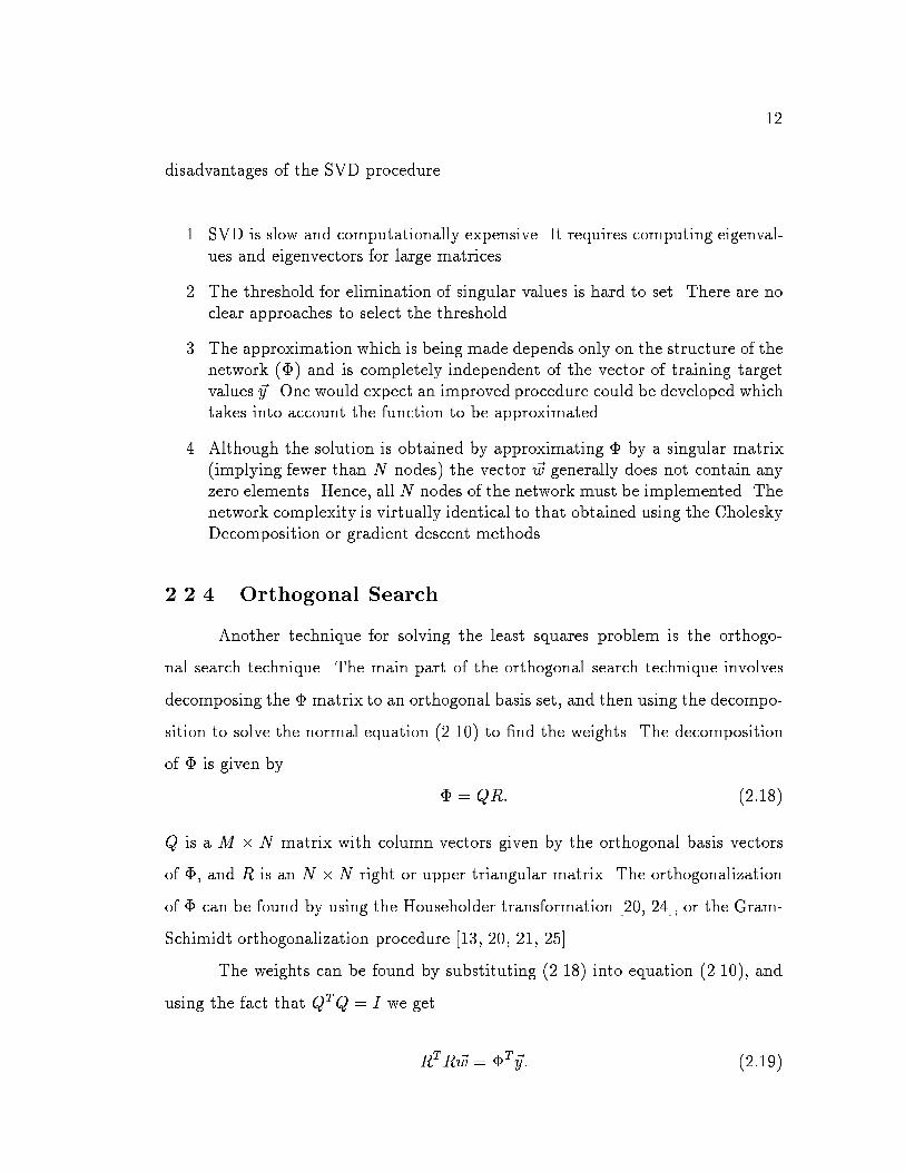
12disadvantages of the SVD procedure.1. SVD is slow and computationally expensive. It requires computing eigenval-ues and eigenvectors for large matrices.2. The threshold for elimination of singular values is hard to set. There are noclear approaches to select the threshold.3. The approximation which is being made depends only on the structure of thenetwork (�) and is completely independent of the vector of training targetvalues ~y. One would expect an improved procedure could be developed whichtakes into account the function to be approximated.4. Although the solution is obtained by approximating � by a singular matrix(implying fewer than N nodes) the vector ~w generally does not contain anyzero elements. Hence, all N nodes of the network must be implemented. Thenetwork complexity is virtually identical to that obtained using the CholeskyDecomposition or gradient descent methods.2.2.4 Orthogonal SearchAnother technique for solving the least squares problem is the orthogo-nal search technique. The main part of the orthogonal search technique involvesdecomposing the � matrix to an orthogonal basis set, and then using the decompo-sition to solve the normal equation (2.10) to �nd the weights. The decompositionof � is given by � = QR: (2:18)Q is a M � N matrix with column vectors given by the orthogonal basis vectorsof �, and R is an N �N right or upper triangular matrix. The orthogonalizationof � can be found by using the Householder transformation [20, 24], or the Gram-Schimidt orthogonalization procedure [13, 20, 21, 25].The weights can be found by substituting (2.18) into equation (2.10), andusing the fact that QTQ = I we getRTR~w = �T~y: (2:19)

13The above equation can be solved for the weight vector by the method of forwardsubstitution, and backward substitution [20] as described in section 2.2.2.This procedure does not work when � is singular, and it does not give anyinsight about the network structure. A more useful approach is to use the orthog-onal basis vectors to choose a set of nodes which reduces some error criteria forsolving the least squares problem. Chen [13] presents one such algorithm, derivedfrom the Gram-Schimidt procedure, to select the most `signi�cant' nodes one byone. In [14] a similar algorithm was also presented to select basis function oneby one, with emphasis on the characterization of nonlinear systems with randominputs. Korenberg et. al. [14] presents an improved, fast version of the orthogonalsearch technique described in [26].During each step of Chen's algorithm [13], the following procedure is usedto search a set of candidate nodes to determine which node will be added to thecurrently selected set.1. For each candidate, �nd the component of the basis vector associated withthat node which is orthogonal to all of the currently selected nodes. Eitherthe Gram-Schimidt or the Householder technique may be used. Call thiscomponent ~qi.2. For each candidate, evaluate the projection of the target vector ~y onto theunit vector in the direction of the orthogonal componentpi = ~yT ~qik~qik : (2:20)This component gives the length of the change in ~y which will result if theith vector is added to the currently selected set.3. Choose the node which gives the largest value of pi - this is the node whichwill provide the greatest reduction in the mean-square error.

14The importance of choosing the nodes one by one is signi�cant in severalaspects. The following is a list of some advantages.1. Selection of nodes one by one provides an insight to the approximation prob-lem, and the network structure. This insight can be used to further modifythe network.2. This selection procedure will let us meet some physical limitations. Nodesmean connections, so a reduction of nodes will provide a corresponding re-duction of connections which can be very useful for hardware applications.3. This procedure does not involve the selection of an arbitrary thresholdinglike the SVD method which can a�ect our solution. The desired number ofnodes can be easily chosen just by looking at the error behavior.The orthogonal search method is very useful, but not so practical. Themethod has not been widely accepted primarily because of the computational com-plexity. The procedure is not generally practical for networks of reasonable size.However, the above algorithm may be shown to be extremely redundant making itcomputationally expensive. In chapter 3 an algorithm will be presented to imple-ment the orthogonal search technique e�ciently. The algorithm will perform thesame orthogonalization procedure without explicitly calculating the orthogonal setmaking it much easier to implement.

15CHAPTER 3The Fast Orthogonal SearchIn chapter 2 some traditional approaches to solve the least square problem werediscussed. The techniques discussed have a variety of problems for �nding theweights for a RBF network. A major issue that had been left untouched is that ofhow many nodes are really needed to train a RBF network and what is the jus-ti�cation. Several clustering algorithms [6, 7, 12, 27] have been developed whichcould reduce the number of nodes, but these clustering algorithms by no meanssuggest whether the network will converge to a stable set of weights or not. Inthis chapter a simple, fast algorithm will be developed to �nd a set of weights thatare best for the given network, and this solution of weights will indeed suggest thenumber of nodes needed by the network. The procedure may be shown to be acomputationally e�cient procedure for implementing the orthogonal search tech-nique of section 2.2.4. Similar fast orthogonal search techniques have been usedby Korenberg [14, 15] for time-series analysis, system identi�cation, and signalidenti�cation problems.In section 3.1 the fast orthogonal search technique will be developed math-ematically. In section 3.2 a simple algorithm will be presented to implement thetechnique. A summary of computational requirements will be given in section 3.3.3.1 Mathematical DevelopmentThe problem of solving for the RBF weights from the equation (2.3) is theissue of this section. Like the orthogonal search technique, during each iterationof the algorithm a set of candidate nodes will be considered to identify which nodewill provide the best improvement to the approximation of ~y. This node will beadded to the network, and the procedure continues until either an error criterion

16is met or the number of nodes in the network reaches a desired value. Unlike theorthogonal search technique, the orthogonal basis set associated with the selectedset of nodes is never explicitly calculated, signi�cantly reducing the computationalburden of the procedure. The Cholesky decomposition discussed in section 2.2.2is the backbone of the proposed fast orthogonal search. Let's de�ne ~�j as the Melement column vector representing the output of the jth node for M number ofsamples. If the job is to consider each node individually, let's also de�ne n~�jo asthe set of node functions to be considered, and let � denote the matrix containingthe ~�j for the currently selected nodes. Let �T� have Cholesky decomposition�T� = UTU . If a candidate function ~�j 2 n~�jo is added to the � matrix, theCholesky decomposition will be modi�ed by264 �T~�Tj 375 � � ~�j � = 264 UT 0~xTj �j 375264 U ~xj0 �j 375 ; (3:1)where 264 ~xj�j 375 denotes the new column of the U matrix. For the time being, assumethat ~xj and �j are known for each ~�j 2 n~�jo. (We must still show how ~xj and �jshould be updated as the � matrix changes.)To select the appropriate ~�j, we need to look at how the selection of anode changes the estimate of ~y, ~y. We prefer to select nodes which produce largechanges in ~y. For the modi�ed � of the above equation, the normal equation ofthe form (2.10) can be written as264 �T~�Tj 375 � � ~�j � ~wj = 264 �T~�Tj 375~y: (3:2)By using the decomposition of equation (3.1) in the above equation, we obtain

17264 UT 0~xTj �j 375264 U ~xj0 �j 375 ~wj = 264 �T~y~�Tj ~y 375 : (3:3)As before in Cholesky decomposition equation (3.3) can be solved for ~zj by themethod of forward substitution where ~zj is~zj = 264 U ~xj0 �j 375 ~wj : (3:4)Applying forward substitution in equation (3.3), we obtain~zj = 264 ~z01�j (~�Tj y � ~xTj ~z0) 375 ; (3:5)where ~z0 (from UT~z0 = �T~y) is the old solution for ~z and is the same for all the~�j candidates. So the only change in ~zj due to adding ~�j is the addition of the thelast component of the vector. Notice that this term is a scalar quantity and forsimplicity let's de�ne �j = ~�Tj y � ~xTj ~z0: (3:6)Now the estimate for the weights can be found by solving264 U ~xj0 �j 375 ~wj = 264 ~z0�j�j 375 : (3:7)We de�ne the changes in ~wj, �~wj, using the equation~wj = 264 ~w00 375+ � �~wj � ; (3:8)where ~w0 is the solution to �T�~w0 = �T~z0 before � is modi�ed (U ~w0 = ~z0). This

18gives 264 U ~xj0 �j 375�~wj = 264 0�j�j 375 : (3:9)The new estimate of ~y is then,~yj = � � ~�j � ~wj = ~y0 + � � ~�j ��~wj; (3:10)where ~y0 = �~w0 is the old estimate. Let's de�ne �~yj = [� ~�j]�~wj. The bestnode to select out of n~�jo is the node which contributes the most to the ~y (hasthe largest �~y). The length squared of �~y isk�~yk2 = �~yTj �~yj = �~wTj 264 �T~�Tj 375 � � ~�j ��~wj: (3:11)Now, by substituting the modi�ed Cholesky decomposition of equation (3.1) in theabove equation we get,k�~yjk2 = �~wTj 264 UT 0~xTj �j 375264 U ~xj0 �j 375�~wj: (3:12)Taking a step farther and applying equation (3.9) to the above equation we getk�~yk2 = 264 U ~xj0 �j 375�~wj 2 = 264 0�j�j 375 2 = �2j�2j : (3:13)Rewritting the above equation, k�~yjk2 = �2j�2j : (3:14)The equation (3.14) is very important since it determines how much im-provement we get by adding the new node ~�j. This equation will be the decision

19criterion for including a node. So if we have to choose from the collection f~�jg,the wisest choice would be to choose the node that gives the largest value of �2j=�2j .Now we need to �nd how all the �i, �i, and xi changes as � gets updated by a node.To describe the updating rules, we introduce the following notation. Anyquantity with ~ on top denotes the updated version of that quantity. That is, ~? isthe value of ? after ~�k has been added to the � matrix. Here ? can be a matrix,a vector or a scalar quantity, and ~�k is the kth node that has been selected to bethe best choice from the set f~�jg. So using this notation we have,~� = � � ~�k � ;~U = 264 U ~xk0 �k 375 :We need to �nd ~�j, ~�j , and ~~xj in terms of �j, �j, ~xj, �k, �k, and ~xk.The terms ~�j and ~~xj form the Cholesky Decomposition of the Gram matrixafter the modi�cation: that is by multiplying out the form of equation (3.1)264 ~�T ~� ~�T ~�j~�T ~�j ~�Tj ~�j 375 = 264 ~UT ~U ~UT ~~xj~~xTj ~U ~�2j + ~~xTj ~~xj 375 : (3:15)To get ~~xj we must solve, ~UT ~~xj = ~�T ~�j, that is,264 UT 0~xTk �k 375 ~~xj = 264 �T~�Tk 375 ~�j: (3:16)By using the methods of forward substitution and using the fact that ~xj is the

20solution to UT~xj = �T ~�j, we get~~xj = 264 ~xj1�k (~�Tk ~�j � ~xTk ~xj) 375 : (3:17)For simpli�cation the last component of ~~xj will be called �j, i.e. �j = 1�k (~�Tk ~�j �~xTk ~xj). We obtain ~�i by using the last equation (~�2j + ~~xTj ~~xj = ~�Tj ~�j) of (3.15),~�2j = ~�Tj ~�j � ~~xTj ~~xj= ~�Tj ~�j � ~xTj ~xj � �2j~�2j = �2j � �2j ; (3:18)where �2j = ~�Tj ~�j � ~xTj ~xj is the value before ~�k is added to �.Finally ~�i can be found from equation (3.6):~�j = ~�Tj ~y � ~~xTj ~~z0= ~�Tj ~y � � ~xTj �j � 264 ~z0�k�k 375= ~�Tj ~y � ~xTj ~z0 � �k�j�k~�j = �j � �k�j�k ; (3:19)where �j = ~�Tj ~y � ~xTj ~z0.The development of the fast orthogonal search comes down to only fourimportant equations: (3.14, 3.17, 3.18, 3.19), these equations are boxed above. Toselect nodes one by one, we look �rst at the equation (3.14) to get the highestcontributor, and then update the important terms of equations (3.17, 3.18), which

21are also terms in U , due to inclusion of the most important node, and �nallyupdate (3.19) so that the next important node can be selected. This selectionprocess can keep repeating until the desired number of nodes has been selected, oran error criterion has been met for the estimate. In the next section a very simplealgorithm will be presented to implement it to �nd the weights.3.2 Fast Orthogonal Search AlgorithmIn section 3.1 the mathematical background was given for the fast orthogo-nal search technique. Even though the development of the technique looks compli-cated, the implementation of the technique is not so. In this section an algorithmwill be presented for the technique, which will make it much easier to implement.The most important equations that we need to worry about are the ones boxed insection 3.1. Let's look at the RBF equation (2.3) of the matrix form again,~y = �~w: (3:20)We need to solve this equation for weights ~w. The matrix � = [~�1~�2 � � � ~�N ] is theoutput of all N nodes for M samples. For the orthogonal search the nodes (or thecolumns ~�i) will be added one by one in an order such that the node which giveshighest improvement, as in equation (3.14), is given the highest preference. Thefollowing algorithm presents the appropriate steps to implement the technique.1. Put all the columns of � (~�i's) in the set f~�jg.Initialization of some variables by setting,�i = ~�Ti ~y;�2i = ~�Ti ~�i;xi = [0 � 1 vector] ;U = [0 � 0 matrix] ; (3.21)

22where, i = 1; 2; � � � ; N ,Set Error = ~yT~y, and Number node selected = 0.2. The iteration begins here.Find the maximum value of �2i =�2i for all i. Let's say the maximum is ati = k.3. Now set, ~U = 264 U ~xk0 �k 375 : (3:22)4. Now we update the ~xi as in equation (3.17), by �nding �i �rst,�i = 1�k (~�Tk ~�i � ~xTk ~xi) (3:23)and then, ~~xi = 264 ~xi�i 375 : (3:24)5. We also need to update �i as in equation (3.18),~�2i = �2i � �2i : (3:25)6. Finally we update � as in equation (3.19) by,~�i = �i � �k�i�k : (3:26)In the above, from step 4 to step 6 updating is only required when i 6= k.7. Keep repeating from step 4 through step 6 until all the nodes in the set f~�jghave been updated.

238. Delete the kth node from the set f~�jg.9. Increment the Number node selected by one, and set Error = Error ��2k=�2k . If Error is less than some error threshold, or theNumber node selectedis equal to the desired number of nodes then go to step 10, otherwise gothrough the steps 2 - 8 again.10. At this stage we have a U matrix giving the Cholesky decomposition of ��T� = UTU: (3:27)Note that here � does not contain the response from all nodes as in section2.2.2, � is formed only from the set of nodes that reduce the sum squarederror of ~y. We can use the equation above in the normal equation (2.10), andthen solve for the weights of the selected nodes by the method of forwardsubstitution, and backward substitution.The algorithm presented in this section not only implements the techniqueto �nd the weights of a given network, but also allows the user to select the numberof nodes. This selection has physical signi�cance since there may exist hardwareor software limitations on implementing nodes. The algorithm �nds the best �xednumber of nodes rather than just an arbitrary choice of nodes. If the number ofnodes is not an issue than one may be able to �nd a better network by choosinga sum square error threshold. Also we can look at how the error is behaving asthe nodes have been added to the network. This provides an indication of whetheraddition of a node really makes a di�erence or not. A subroutine which implementsthe above algorithm is included in Appendix A.1.

243.3 Computational EvaluationsThis section will compare the procedure of fast orthogonal search techniquepresented in this chapter to the orthogonal search techniques presented in section2.2.4 in terms of computational complexity. Here, the complexity of an algorithmmay be evaluated by counting the number of multiplications required to imple-ment the training procedure. The number of multiplications required for the fastorthogonal search described by Korenberg [14] is given by O(SNM + S3N). HereS is the total number of nodes selected, N is the total number of initial nodes, andM is the total number of training samples. For the Orthogonal search technique ofsection 2.2.4 (developed by Chen [13]) the total number of multiplications requiredis O(S2NM). The fast orthogonal search technique developed in this chapter re-quiresO(SNM+S2N) multiplications. So the fast orthogonal algorithm presentedin section 3.2 is not only simple but also fast. It requires a factor of S fewer com-putations than the method presented in [13], and is either comparable to or fasterthan Korenberg's algorithm of [14].In the next chapter some applications of the RBF network will be given.The technique will also be evaluated against standard techniques, and an analysisof di�erent aspects of the network will be presented.

25CHAPTER 4Applications of the RBF NetworkThe application of RBF neural networks is widespread. RBF networks have beensuccessfully applied in pattern recognition [3, 6, 7], function approximation [8], timeseries prediction [8], signal detection [9, 28] and many other important problems.In this chapter, several applications of the RBF network using the fast orthogonalsearch for training will be given, and an analysis of the performance of the networkwill be provided.In section 4.1 the application of RBF networks in analog to digital converter(ADC) error compensation will be presented. In section 4.2 a simple patternrecognition problem will be handled, and �nally in section 4.3 the application tochromosome classi�cation will be presented.4.1 Analog to Digital Converter Error CompensationThe error compensation of ADC's has been undergoing research for severalyears [29]. Although the error introduced by an ADC is much smaller than thesignal amplitude in general, the compensation of an ADC may be used to improvethe linearity of the converter. For many spectral analysis and signal processingapplications, the linearity of the converter is a critical speci�cation. Despite theheavy growth of neural networks, few have attempted compensation using neuralnetworks.4.1.1 Problem DescriptionThe error correction for an ADC is to eliminate frequency dependent dis-tortion introduced by the converter [30]. To cope with this frequency dependentdistortion Hummels et. al. [30] present a dynamic compensation procedure. Thisdynamic compensation was based on the the converter output and some estimate

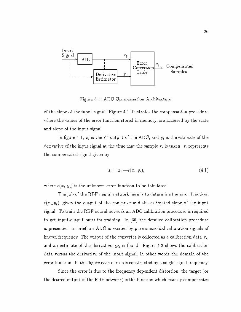
26CorrectionErrorTableEstimatorDerivativeSignalInput CompensatedSamples- -?- --ADC xy zii iFigure 4.1: ADC Compensation Architectureof the slope of the input signal. Figure 4.1 illustrates the compensation procedurewhere the values of the error function stored in memory, are accessed by the stateand slope of the input signal.In �gure 4.1, xi is the ith output of the ADC, and yi is the estimate of thederivative of the input signal at the time that the sample xi is taken. zi representsthe compensated signal given byzi = xi � e(xi; yi); (4:1)where e(xi; yi) is the unknown error function to be tabulated.The job of the RBF neural network here is to determine the error function,e(xi; yi), given the output of the converter and the estimated slope of the inputsignal. To train the RBF neural network an ADC calibration procedure is requiredto get input-output pairs for training. In [30] the detailed calibration procedureis presented. In brief, an ADC is excited by pure sinusoidal calibration signals ofknown frequency. The output of the converter is collected as a calibration data xi,and an estimate of the derivative, yi, is found. Figure 4.2 shows the calibrationdata versus the derivative of the input signal, in other words the domain of theerror function. In this �gure each ellipse is constructed by a single signal frequency.Since the error is due to the frequency dependent distortion, the target (orthe desired output of the RBF network) is the function which exactly compensates

27

0 50 100 150 200 250-400

-300

-200

-100

0

100

200

300

400

state

slop

e

The calibration data

Figure 4.2: The domain of the error function.

28the harmonics which exist in the calibration data. The above described problemcan be represented by F�(~x; ~y)~w = F~x: (4:2)Here, F represent a Fourier Transform (FT) matrix, �(~x; ~y) is the matrix form ofthe output of the RBF nodes, and ~x and ~y are the calibrated state data and theestimate of the derivative respectively. ~w is the weight vector of the RBF network.For a more detailed discussion on equation 4.2, see [30].4.1.2 ResultsCalibration data was collected from a Tektronix AD-20 8-bit converter sam-pling at 204.8 megasamples per second (MSPS). The data was then presented toa RBF network to learn the harmonics. The RBF nodes of the network wereplaced on training samples which were separated by a �xed minimum distance.The covariance for each node is chosen to be diagonal with diagonal elements pro-portional to the separation distance of the nodes. The � matrix of the networkwas constructed as in equation (4.2) with 300 nodes. Finally the weights of thenetwork were found by the fast orthogonal search technique presented in Chapter3. The technique of orthogonal search was used to �nd the best 50 nodes and theirweights.After training, an error table was constructed using the estimated functione(x; y). Figure 4.3 shows the constructed error table. To evaluate the performanceof the table a measure of Spurious Free Dynamic Range (SFDR) was evaluated.The SFDR was found by measuring the dB di�erence between the height of thefundamental and the height of the highest spurious signal in the spectrum of theADC output as illustrated in Figure 4.4.This measure is not a simulation, it is an actual measure done using a highperformance test bed and the same AD-20 converter. Raw data was collected bydriving the converter with a pure sinusoidal signal, and was compensated using

29

0

100

200

300

-400

-200

0

200

400-1

-0.5

0

0.5

1

stateslope

wahid 21:44 7/19/94 Figure 4.3: An error table.

30

0 20 40 60 80 100-40

-20

0

20

40

60

80

frequency (MHz)

mag

nitu

de o

f FF

T

SFDR

Figure 4.4: Measure of SFDR.

31the table built by the RBF network as in (4.1).Figure 4.5 shows the SFDR versus various test frequencies. The table iscompensating the error by 10 dB or better throughout the Nyquist band. Forcomparison, a table was built using the same RBF network structure, but theweights were found using the method of Singular Value Decomposition (SVD)discussed in Section 2.2.3. The SFDR for the SVD technique is also shown in the�gure 4.5. Even though the SFDR for both SVD technique and orthogonal searchtechnique are similar, the orthogonal technique has some added advantages. Theorthogonal technique is less time consuming than the SVD technique since theSVD technique requires �nding the eigenvalues and eigenvectors of large matrices.The orthogonal technique gives the same performance with fewer nodes, providinga way to discard the unimportant nodes. If we look at the sum squared error asa node gets added in, we can make an intelligent decision about whether to addmore nodes or not.Figure 4.6 shows how the error function decreases as each node is added intothe network. From this plot it is obvious that it may not improve the performanceat all after the 30th node had been added. In comparison, use of the SVD techniquerequires inclusion of all 300 nodes.For many problems, insight into the importance of various nodes may begained by examining the sequence with which nodes are added to the network.Figure 4.7 illustrates this selection process. The initial nodes are presented in the�gure by `o' and the selected nodes are presented by `�'. Next to each selected node,a number is printed which indicates the order in which the nodes are selected. This�gure demonstrates the most important regions of the domain of this problem.To get a better insight into the problem, a di�erent procedure was usedto place the initial nodes. The node centers of a RBF network were placed inlayers of arrays of nodes. The �rst layer includes only 4 nodes on 4 corners ofthe input space of the ADC calibration data. 4� 4 array of nodes were placed on

32

0 20 40 60 80 10040

45

50

55

60

65

70

frequeny (MHz)

SF

DR

wahid 16:12 7/14/94

uncompensated

compensated using SVD method

compensated using FOS method

Figure 4.5: SFDR for the uncompensated, compensated by proposed technique,and compensated by singular value decomposition.

33

0 10 20 30 40 500.1

0.15

0.2

0.25

0.3

0.35

0.4

basis function added in

erro

r

wahid 16:22 7/14/94Figure 4.6: The sum squared error for the network as each node gets added in.

34

0 50 100 150 200 250-400

-300

-200

-100

0

100

200

300

400

state

slop

e

001

002

003

004

005

006

007

008

009

010

011

012

013

014

015

016

017

018

019

020

021

022023

024

025

026

027

028

029

030

031032

033

034

035

036

037

038

039

040

041

042

043

044

045

046

047

048049

050

wahid 21:53 7/19/94Figure 4.7: The selection of 50 nodes out of 500 initial nodes.

35the second layer, 8 � 8 array of nodes were placed on the third layer, and �nally16�16 array of nodes were placed on the last layer. The covariance matrix of eachnode was made diagonal with the diagonal elements given by the distance betweentwo neighboring nodes of the same layer. This node placement scheme providesthe network with the opportunity to give the error table general shape using thewidely spaced node of layers 1,2 and 3, and �ne structure using the nodes of layer4. Figure 4.8 presents the above described scheme. Here the initial nodes areshown using `.', and the selected nodes are shown using `o'. Notice that the �rst11 nodes were selected from layers 2 and 3 to give the table a general shape, andthen the remaining 39 nodes were selected from layer 4 to provide the required �nestructure of the table. No nodes were selected from layer 1 since the nodes wereoutside the domain of ADC (�gure 4.2).

360 100 200 300

-400

-200

0

200

400

state

slop

e

layer 1

0 100 200 300-400

-200

0

200

400 01

02

state

slop

e

layer 2

0 100 200 300-400

-200

0

200

400

03

04

05

06

07

08

09

10

11

state

slop

e

layer 3

0 100 200 300-400

-200

0

200

400

1213

1415

16

17

18

19

20

21

2223

24

25

26

27

28

29

3031

3233

34

35

3637 38

39

40

4142 43

44

45

46

4748

49

50

state

slop

e

layer 4

Figure 4.8: The selection of 50 nodes out of the 4 layered nodes.

374.2 A Simple Pattern Recognition ProblemFrom the signal processing application of the previous section, this sectionmoves to a pattern recognition problem which is much more familiar territory forneural networks. The problem here is to classify simple two dimensional, and twoclass patterns. A training set of 400 samples were generated as Gaussian randomvectors. The �rst class (class `0') are zero mean random vectors, with an identity(I) covariance matrix. The second class (class `1') has mean vector [1 2]T , and adiagonal covariance matrix with diagonal elements 0.01 and 4.0. Figure 4.9 showsthe training data set described above. Here `o' is used for class 0, and a `+' isused for class `1'. A test set of 20000 samples was also generated using the sameGaussian density parameters. The reason for choosing this example is that it hasbeen used by several researchers to evaluate various neural network classi�cationschemes [6, 7, 16, 27, 31].The RBF network presented here was trained using the 400 training sam-ples. The nodes of the network were placed on the 400 training samples and allthe nodes had the same covariance matrix �2I, where sigma is the width chosenbetween 0.1 and 1. The network was asked to �nd 50 best nodes, and their weights.The desired network output was set to zero for any class `0' sample, and one forclass `1' samples. After training, the network was tested with the 20000 test sam-ples. Figure 4.10 gives the percentage error versus the width of a node �. Theminimum error was found to be 7.92% when the � was 0.4. The minimum errorgiven by [6] was 9.26%, and the optimal error for this problem using a quadraticclassi�er was 6% [6]. So the network presented here not only outperforms thestandard RBF approaches [6, 27], but also requires fewer nodes. In [6] the 9.26%error was obtained by using 86 nodes, and all the nodes had di�erent covariancematrices. The Fast Orthogonal Search technique found the 50 best nodes and theirweights in less than 2 minutes in a DEC3100. So the speed of training is also verygood.

38class 0class 1

-3 -2 -1 0 1 2 3-4

-2

0

2

4

6

8

x1

x2

The training data of the 2 dimensional 2 class problem

Figure 4.9: The training sample for the 2D 2-class problem.

39

0 0.2 0.4 0.6 0.8 15

6

7

8

9

10

11

12

13

14

15

sigma

perc

ent e

rror

Error vs Sigma for 2 dimensional problem

<----- RBF percent error

optimal error

Figure 4.10: The percentage error vs � for the 2D 2-class problem.

40To see how the RBF network is generalizing over the entire domain, �gure4.11 shows the output surface of the network over the entire domain of the inputsample.The behavior of the sum square error on the training sample is also anissue of our discussion. Figure 4.12 shows how the error is decreasing as eachnode gets added in. Again as in the previous section the sum square error on thetraining sample becomes almost at as the `signi�cant' nodes have been added.Finally a plot is presented here which shows how the search technique selected the`signi�cant' nodes from the whole set. Figure 4.13 shows the 50 nodes selectedby the network, and their order of selection. From this plot we can see that the�rst node was picked from a pure class 0 region, and the second node was pickedfrom the pure class 1 region, which makes complete sense since we want the mostimportant nodes to be where most of training samples are. Also from �gure 4.12we can see that the introduction of the �rst node reduces training error by 50%.

41

-5

0

5

-5

0

5

100

0.2

0.4

0.6

0.8

1

x1x2

netw

ork

outp

ut

The output error surface for the 2 class problem

Figure 4.11: The output surface of the RBF for the 2D 2-class problem.

42

0 10 20 30 40 500

20

40

60

80

100

120

140

160

180

200

basis function added in

sum

squ

are

erro

r

wahid 11:56 7/15/94Figure 4.12: The sum squared error of the training samples for the 2D 2-classproblem.

43

-2 -1 0 1 2 3-2

-1

0

1

2

3

4

5

x1

x2

50 best nodes selected out of 400, and their order of selection

1

2

3

4

5

6

7

8

9 10

11

12

13

1415

16

17

18

19

20

21

22

23

24

25

26

27

2829

30

31

32

33

34

35

36

37

38

39

40

41

42

43

44

45

46

47

48

49

50

Figure 4.13: The node selection process of the orthogonal search technique.

444.3 Classi�cation of ChromosomeA more complicated and challenging application of RBF will be discussed inthis section. \Karyotyping", the classi�cation of the chromosome in a metaphaseinto the 24 normal classes has been a very important issue in the medical �eldfor many many years. However, the automation of karyotyping by computers hasbeen in development only for about 25 years [32]. Classi�cation of chromosomesinvolves �nding a good set of features to describe a chromosome, and a classi�cationtechnique to identify the chromosomes using the features. The RBF neural networkdeveloped in this report will be used for the classi�cation of chromosome given aset of features.4.3.1 RBF Network for Chromosome Classi�cationThe problem of karyotyping involves classifying the chromosome of ee fea-tures (for the data base used here) into 24 di�erent classes. The chromosomes ina cell consists of 22 pairs of autosomes, one of each pair inherited of each parent,and two sex chromosomes (an X and Y for male, and two X's for female). Classi-�cation of a cell correctly requires classi�cation of all 24 classes of a cell. Ratherthan classifying a cell, this report will look at the classi�cation per class. So herethe problem is to only classify each pair of autosomes, and the sex chromosomes.The RBF structure for the chromosome classi�cation is slightly di�erentthan the one given in Section 2.1. The output layer of the network consists of 24output nodes to classify the 24 classes. The decision of the network is the node thatgives highest output. One major advantage of the fast orthogonal search techniquewill be evident here. Figure 4.14 illustrates the RBF network for chromosomeclassi�cation. In standard RBF networks, all the nodes of the hidden layer areconnected to all the nodes of the output layer. The fast orthogonal search will beable to reduce the insigni�cant connections. The reduction of the nodes can be ofvery large scale for a multiclass problem like the chromosome classi�cation. The

45

MUMIXAM

1

2

N

2

24

output

x

1layer to the output layerconnected from the hiddenOnly p nodes are

Figure 4.14: Network structure for the RBF Network for Chromosome Classi�ca-tion.

46following result and analysis section will show this phenomenon.4.3.2 Results and AnalysisThe chromosome database used for evaluating the method is the Philadel-phia database [32, 33, 34]. Each pattern of this database is an autosome, the Xsex chromosome, or the Y sex chromosome. Each pattern consists of a set of 30di�erent features, which are the measurements of the normalized area, size, den-sity, normalized convex hull perimeter, normalized length, area, centromeric index,mass centromeric index, length centromeric index, the weighted density distribu-tion density, and others [34].The RBF neural network was trained with 1000 training patterns. Theinitial nodes of the network were placed on these 1000 patterns. The covarianceof each node was chosen to be diagonal with initial diagonal elements equal to theestimated variance of the class the node belongs to, that is�2ik = E n(xjk � cik)2o ~xj;~ci 2 fclass lg: (4:3)Where �2ik denotes the kth diagonal element of the covariance matrix �i for theith node, and cik is the kth component of the ith node center, and xjk is the kthfeature of the pattern ~xj. The diagonal elements of the covariance matrix wereadjusted to separate the closest discriminating nodes. The adjustment was madeby multiplying the diagonal element of the covariance matrix by a fraction of thedistance between two overlapping classes, that is�i = �i(~cj � ~ci)T��1i (~cj � ~ci); ~cj;~ci 62 fclass lg: (4:4)Where is a constant less than 1.0. The fast orthogonal search was used to only�nd the best 40 nodes and their weights. The search technique successfully foundthe desired nodes. Figure 4.15 shows the training error for class 1 as each node

47was added in.Notice here that only 40 out of 400 RBF nodes are connected to the output.By looking at �gure 4.15, we see that the training error for class 1 has leveled o�by the introduction of the 40th node, implying that introducing another node maynot improve the performance at all. Similar conclusions can be made for trainingother classes.After training the network, it was tested by a test set of 3000 patternsdi�erent from the training set. The percent error for this test set was 20.87%,which was slightly (1.73%) lower than the ones presented by [32, 33, 34].The number of initial nodes from which to select a set of nodes of thenetwork can in uence the performance. Figure 4.16 illustrates the results of somesimple tests where the number of initial node assignments was changed for thetraining procedure described above. The plots in �gure 4.16 give the percent error(y-axis) for a network constructed by selecting a set of nodes per class from alarger set of initial nodes (x-axis). The test was performed to select 20, 30, 40, 50and 60 nodes per class from the initial sets. The percentage error was generallylower than the error given by [32, 33]. From Figure 4.16 we can also see that thepercent error for 20 selected nodes per class is higher than all other selections.This suggests that 20 nodes per class is not necessarily the best. On the otherhand, selection of 60 nodes does not improve the percent error at all suggestingovertraining. The smaller initial sets of (100-300) nodes are good, but not thebest-too little to choose from, and the percent error increases as the initial nodesincreases-too many to choose from. One other important issue is that even thoughthe percent error is changing due to the selection process, the di�erence betweenthe best performance and the worst performance of all the tests is merely 3.2%,suggesting that the fast orthogonal search procedure is �nding the best possibleselection for a given network.

48

0 10 20 30 400

5

10

15

20

25

30

35

40

45

basis function added in

sum

squ

ared

err

or

wahid 12:12 7/23/94Figure 4.15: The sum squared error for training class 1 of the Chromosome prob-lem.

49

200 400 600 800 100020

21

22

23

24

25

26

initial nodes

perc

ent e

rror

minimum error by PNN (Sweeney)error using 20 selected nodeserror using 30 selected nodeserror using 40 selected nodeserror using 50 selected nodeserror using 60 selected nodes

Figure 4.16: The percent error of the network for di�erent numbers of the initialnode selection

50CHAPTER 5Conclusion5.1 SummaryThis thesis presented an approach to con�gure the most signi�cant compo-nent of the RBF neural networks, the weights.1. The method provides a simple way to �nd the most signi�cant nodes of thenetwork and their weights.2. The technique of fast orthogonal search is implementable using a simple 10step algorithm. Traditional approaches require signi�cantly more computa-tions.3. The technique provides a solution regardless of the network parameters. Theprovided solution is the best to match the target function. The traditionalapproaches may not converge, or may produce an erroneous solution.4. The solution is correlated with the target function, so scaling of any node willnot a�ect the network output. This is in contrast to many of the traditionalapproaches, where node activation functions must be carefully normalized.5. The approach gives a clear indication of the number of nodes to be used.Nodes should be added only until addition of a node does not improve theoutput signi�cantly.6. Several important applications of the RBF network have been provided. Theresults show that the orthogonal search technique gives better performancethan that of other approaches.

515.2 Future WorkThe fast orthogonal search technique is a signi�cant improvement over exist-ing RBF training techniques. The method provides good insight into the concernedproblem, and the size of the network required to address the problem. However,additional research could make the procedure more practical to implement, or moreadaptable to complex problems.The �rst issue is that if the problem is too big and requires a large network,we must contend with memory limitations. For example, if we want to train thechromosome problem of chapter 4 with 2000 training samples, and 1000 initialnodes, then the size of the � matrix is very large (2000� 1000� 8bytes � 16MB).It's almost impossible to implement a problem of this size. To solve this problemwe have to look at how we can implement this technique without having to storethe large matrix. It may be necessary to generate the columns of � again andagain to solve the problem.The second issue is that after we �nd the most signi�cant node ~�k fromthe set f�jg, is there anything we can do to make it even better? One possibilitywould be to optimize the node by changing its width �. The work presented inthis thesis may provide some insight into this problem, since speci�c equations aregiven which relate the vector ~� to the improvement in LS solution.Finally, some more applications of the RBF network can be used to evalu-ate the procedure. For example Optical Character Recognition (OCR) is a goodproblem for neural network. The problem of handwritten zipcode recognition [35]can be a challenge for the fast orthogonal search technique.

52REFERENCES[1] D.E. Rumelhart, J.L. McClelland, Parallel Distributed Processing, MIT Press,Cambridge, MA 1986.[2] D.S. Broomhead, D. Lowe, \Multivariable Functional Interpolation and Adap-tive Networks," Complex Systems, vol. 2, pp. 321-355, 1988.[3] J. Moody, C.J. Darken, \Fast Learning in Networks of Locally Tuned Process-ing Units," Neural Computation, vol. 1, pp. 281-294, 1989.[4] D.F. Specht, \A Generalized Regression Neural Network" IEEE Transactionsof Neural Networks, vol. 2, No. 6, pp. 568-576, 1991.[5] T. Kohonen, \The Self Organizing Map", Proceedings of IEEE, vol.78, No. 9,pp.1464-1480, 1990.[6] M.T. Musavi, W. Ahmed, K.H. Chan, K.B. Faris, D.M. Hummels, \On theTraining Algorithm for Radial Basis Function Classi�ers," Neural Networks,vol. 5, pp. 595-603, 1992.[7] K. Kalantri, Improving the Generalization ability of Neural Network Classi�ersM.S Thesis, University of Maine, Orono, Maine, May 1992.[8] R. D. Jones, Y. C. Lee, W. Barnes, G. W. Flake, K. Lee, P. S. Lewis, S. Qian,\Function approximation and Time Series Prediction with Neural Networks,"Proc. of the IJCNN, pp 649-665, June 1990.[9] W. Ahmed, D.M. Hummels, M.T. Musavi, \Adaptive RBF Neural Detectionin Signal Detection," Proccedings of International Symposium on Circuits andSystems (ISCAS '94), pp 265-268, May 29 - June 2, 1994, London, U.K.

53[10] L. Xu, A. Krzyzak, A. Yuille, \On Radial Basis Function Nets and KernelRegression: Statistical Consistency, Convergence Rates, and Receptive FieldSize", Neural Networks, vol. 7, No. 4, pp. 609-628, 1994.[11] S. Chen, B. Mulgrew, P.M. Grant, \A clustering technique for Digital Commu-nications Channel Equalization Using Radial Basis Function Networks" IEEETransactions on Neural Networks, vol. 4, No. 4, pp. 570-579, Mar. 1993.[12] H. Spath, Cluster Analysis Algorithms for Data Reduction and Classi�cationof Objects, Halstead Press, 1980, New York.[13] S. Chen, C.F.N. Cowan, P.M. Grant, \Orthogonal Least Squares LearningAlgorithm for Radial Basis Function Networks" IEEE Transactions on NeuralNetworks, vol. 2, No. 2, pp. 302-309, Mar. 1991.[14] M.J. Korenberg, L.D. Paarmann, \Orthogonal Approaches to Time-SeriesAnalysis and System Identi�cation," IEEE SP Magazine, July 1991, pp. 29-43.[15] L.D. Paarmann, M.J. Korenberg, \Accurate ARMA Signal Identi�cation -Empirical Results," Proceedings of Midwest Symposium, pp 110-113,1991.[16] M.T. Musavi, K.H. Chan, K. Kalantri, W. Ahmed, \A MinimumError NeuralNetwork," Neural Networks, vol. 6, pp. 397-407, 1993.[17] K.H. Chan, A Probabilistic Model For Evaluation of Neural Network Classi-�ers M.S Thesis, University of Maine, Orono, Maine, May 1991.[18] W.P. Jones, J. Hoskins, \Back Propagation - A General Delta Learning Rule,"Byte, pp. 155-162, Oct. 1987.[19] H. Guo, S.B. Gelfand, \Analysis of Gradient Descent Learning Algorithms forMultilayer Feedforward Neural Networks", IEEE Transactions on Circuits andSystems, vol. 38, No. 8, pp. 883-893, 1991.

54[20] L.L. Scharf, Statistical Signal Processing, Detection, Estimation, and TimeSeries Analysis, Addision-Wesley Inc., 1991.[21] R. A. Horn, C. A. Johnson, Topics in Matrix Analysis, Cambridge UniversityPress, 1991.[22] G. Sewell The Numerical Solution of Ordinary and Partial Di�rential Equa-tions, Academic Press, INC., San Diego, CA, 1988.[23] G. Strang, Linear Algebra and Its Application, Academic Press, 1976, NewYork.[24] R. A. Horn, C. A. Johnson, Matrix Analysis, Cambridge University Press,1985.[25] N. Weiner, Nonlinear Problems in Random Theory, The Technology Press ofMIT and John Wiley & Sons, Inc., New York, 1958.[26] A.A. Desrochers, \On An ImprovedModel Reduction Technique for NonlinearSystems" Automatica, vol. 17, pp. 407-409, 1981.[27] M.T. Musavi, K.B. Faris, K.H. Chan, W. Ahmed, \A Clustering Algorithm forImplementation of RBF Technique," International Joint Conference on NeuralNetworks, IJCNN '91, Seattle, WA, July 1991.[28] D.M. Hummels, W. Ahmed, M.T. Musavi, \Adaptive Detection of Small Si-nusoidal Signals in Non-Gaussian Noise using a RBF Neural Network," to bepublished in 1994 in IEEE Transactions of Neural Networks.[29] T.A. Rebold, F.H. Irons, \A Phase Plane Approach to Compensation of HighSpeed Analog to Digital Converters" IEEE International Symposium on Cur-cuits and Systems, pp. 455, Philadelphia, 1987.

55[30] D.M. Hummels, F.H Irons, R. Cook, I. Papantonopoulos, \Characterizationof ADCs Using a Non-Iterative Procedure," Proccedings of International Sym-posium on Circuits and Systems (ISCAS '94), May 29 - June 2, 1994, London,U.K.[31] M.T. Musavi, W. Ahmed, K.H. Chan, D.M. Hummels, K. Kalantri, \A Prob-abilistic Model for Evaluation of Neural Network Classi�er," Pattern Recogni-tion, vol. 25, pp. 1241-1251, 1992.[32] W. P. Sweeney Jr., M.T. Musavi, J.N. Guidi\Classi�cation of Chromosomes Using Probabilistic Neural Network", Cytom-etry vol. 16 pp. 17-24, 1994.[33] W. P. Sweeney Jr. Classi�cation of Human Chromosomes Using ProbabilisticNeural Network, M.S Thesis, University of Maine, Orono, Maine, August 1993.[34] J. Piper, E. Granum, \On Fully Automatic Feature Measurement for BandedChromosome Classi�cation", Cytometry vol. 10 pp. 242-255, 1989.[35] L. Sharma, Recognition of Handwritten Zipcodes Using Probabilistic NeuralNetwork, M.S Thesis, University of Maine, Orono, Maine, May 1994.

56Appendix APROGRAM LISTINGA.1 Fast Orthogonal Search/****************************************************************fast_ortho_search.cWahid AhmedJun 26, 1994This routine implements the Fast Orthogonal Searchfor a input matrix.the prototype of this function is:double *fast_ortho_search(MATRIX a, double *y,int TOTAL_BASIS, double err_thres);where, a is a matrix.y = aw;w is the unknown parameters returned by this routine.So w is a vector of weights, the unused nodes have weights 0.TOTAL_BASIS is number of nodes desired from the a matrix.err_thres is the sum squared training error threshold to quit.*****************************************************************/#include <stdio.h>#include <math.h>#include "vecmath.h"#include "cmath.h"#define SQ(x) ((x) * (x)) /* define square macro */#define MAX(a,b) ((a > b) ? a:b) /* define maximum macro */double *fast_ortho_search(MATRIX a,double *y, int TOTAL_BASIS,double err_thres){ /* Define variables */MATRIX U,L; /* matrices for decomposition */int i,j,k;double dummy;

57double *p; /* holds the correlation part */double *q; /* holds the energy reduction part */double *C; /* A pointer for the targets */double **x; /* A double pointer for the additionalvector */double *weight; /* The result goes here */double *temp_vec1,*temp_vec2; /* temporary vectors for various uses */int *selected; /* Array that holds the indeces forselected nodes */int flag = 0;double Maximum = -10;int Max_index;double error; /* The error variable *//* define the routines used */MATRIX realloc_mat(MATRIX A,int new_rows,int new_cols);double dot_prod(double *x, double *y, int length);/* allocate memory for various pointers */p = (double *)calloc(a.cols, sizeof(double));q = (double *)calloc(a.cols, sizeof(double));weight = (double *)calloc(a.rows, sizeof(double));temp_vec1 = (double *)calloc(a.rows, sizeof(double));temp_vec2 = (double *)calloc(a.rows, sizeof(double));selected = (int *)calloc(a.cols, sizeof(int));for (i=0;i<a.cols;i++) selected[i] = a.cols + 1;x = (double **)calloc(a.cols, sizeof(double *));for (i=0;i<a.cols;i++)x[i] = (double *)calloc(1,sizeof(double));/* Initialize the weight matrix */for (i=0;i<a.rows;i++) weight[i] = 0.0;/* Initialize the matrix for the result */U = initMatrix(1,1);/* Initialize the correlation and energy values */for (i=0;i<a.cols;i++){

58for (j=0;j<a.rows;j++) temp_vec1[j] = a.el[j][i];p[i] = dot_prod(temp_vec1,y,a.rows);q[i] = dot_prod(temp_vec1,temp_vec1,a.rows);}/* The initial sum squaerd error for the network */error = dot_prod(y,y,a.rows);printf("initial Error = %1.6e\n",error);/* The first iteration */for (i=0;i<a.cols;i++){dummy = SQ(p[i])/q[i];Maximum = MAX(Maximum,dummy);if (Maximum == dummy) Max_index = i;/* printf("Energy = %1.4f for col = %d\n",dummy,i); */}error -= Maximum;/* printf("Error = %1.6e\n",error); */selected[0] = Max_index;U.el[0][0] = sqrt(q[Max_index]);for (i=0;i<a.cols;i++){if (i == Max_index) continue;for (j=0;j<a.rows;j++){temp_vec1[j] = a.el[j][Max_index];temp_vec2[j] = a.el[j][i];}x[i][0] = dot_prod(temp_vec1,temp_vec2,a.rows)/U.el[0][0];q[i] -= SQ(x[i][0]);p[i] -= x[i][0] * (p[Max_index]/sqrt(q[Max_index]));}/* The rest of the iterations */for (i=1;(i<TOTAL_BASIS) & (error > err_thres);i++){/* printf("iteration %d\n",i); */Maximum = -10;/* Find an unselected node that will provide highestimprovement */for (j=0;j<a.cols;j++){

59flag = 0;for (k=0;k<i;k++)if (selected[k] == j){flag = 1; break;}if (flag) continue;if (q[j] <= 1e-50) continue;dummy = SQ(p[j])/q[j];Maximum = MAX(Maximum,dummy);if (Maximum == dummy) Max_index = j;}error -= Maximum;/* printf("Error = %1.6e\n",error); */selected[i] = Max_index;/* First find the Orthogonal decomposition for theselection */U = realloc_mat(U,i+1,i+1);for (j=0;j<i;j++) U.el[j][i] = x[Max_index][j];U.el[i][i] = sqrt(q[Max_index]);/* Update every thing else for selecting the next node */for (j=0;j<a.cols;j++){flag = 0;for (k=0;k<=i;k++)if (selected[k] == j){flag = 1; break;}if (flag) continue;x[j] = (double *)realloc(x[j],(i+1) * sizeof(double));for (k=0;k<a.rows;k++){temp_vec1[k] = a.el[k][Max_index];temp_vec2[k] = a.el[k][j];} x[j][i] = (dot_prod(temp_vec1,temp_vec2,a.rows)- dot_prod(x[Max_index],x[j],i))/U.el[i][i];q[j] -= SQ(x[j][i]);p[j] -= x[j][i] * (p[Max_index]/sqrt(q[Max_index]));}}printf("final Error = %1.6e\n",error);/* for (i=0;i<U.cols;i++) printf("%d\n",selected[i]); *//* The nodes are selected, now find the weights for these

60nodes. Leave the unselected nodes equal to zero *//* This is the constant vector for the linear equation */C = (double *)calloc(U.cols, sizeof(double));for (i=0;i<U.cols;i++){C[i] = 0.0;for (j=0;j<a.rows;j++)C[i] += a.el[j][selected[i]] * y[j];}/* printmatf("%1.4f",U); */L = transpose(U);freeMatrix(U);/* Now solve the system of linear equations by method offorward substitution, and back substitution */if (cholesky_solve(L,C))printf("\nERROR FINDING THE SOLUTION\n");for (i=0;i<L.rows;i++)weight[selected[i]] = C[i];/* Free all the memories */freeMatrix(L);for (i=0;i<a.cols;i++) free(x[i]);free(x);free(p);free(q);free(temp_vec1);free(temp_vec2);free(selected);free(C);return(weight); /* returning the weights */}/***************************************************************realloc_mat.cThis routine reallocates a matrix to a new size, and returns the newmatrix. The values in the old matrix are saved in the new matrixin the same order

61calling sequence:NEW = realloc_mat(OLD, new_rows, new_cols);here,OLD is the OLD Matrix, and NEW is the new one.new_rows and new_cols are the size of the new matrix***************************************************************/MATRIX realloc_mat(MATRIX A,int new_rows,int new_cols){ MATRIX result;int i,j;result = initMatrix(new_rows,new_cols);for (i=0;i<A.rows;i++)for (j=0;j<A.cols;j++)result.el[i][j] = A.el[i][j];freeMatrix(A);return(result);}

62Appendix BPreparation of This DocumentThe author used LaTEX, the high quality typesetting software, to produce thisthesis. Also the drawings were produced by XFIG. The XFIG �les were thenconverted into postscript format or LaTEX format if possible to inlcude in theLaTEX �les. The graphs of chapter 4 were generated using MATLAB.

63BIOGRAPHY OF THE AUTHORWahid Ahmed was born in Dhaka, Bangladesh on November 30, 1969. Hereceived his Higher Secondary Certi�cate (HSC) from Notre Dame College, Dhakain 1986. In 1989 he entered University of Maine majoring in Electrical Engineering,and obtained his Bachelor of Science degree with high distinction in December1992. He had done research in the �eld of neural networks, and pattern recognitionduring last two years of his undergraduate studies. He enrolled in the Master ofScience program in Electrical Engineering at the University of Maine in January1993. He has served as a Teaching/Research Assistant and Assistant NetworkAdministrator in the department of Electrical and Computer Engineering. Hiscurrent research interests are neural networks, image processing, signal processing,pattern recognition, and robotics. He has co-authored several articles in journalsand conference proceedings. He is a candidate for the Master of Science degree inElectrical Engineering from the University of Maine, Orono, in August 1994.

LIBRARY RIGHTS STATEMENTIn presenting this thesis in partial ful�llment of the requirement for anadvanced degree at the University of Maine at Orono, I agree that the Library shallmake it freely available for inspection. I further agree that premission for extensivecopying of this thesis for scholarly purposes may be granted by the Librarian. Itis understood that any copying or publication of this thesis for �nancial gain shallnot be allowed without my written permission.SignatureDate