Vis Comput (2012) 28:553–562DOI 10.1007/s00371-012-0686-z

O R I G I NA L A RT I C L E

Fast optimization-based elasticity parameter estimation usingreduced models

Huai-Ping Lee · Ming C. Lin

Published online: 19 April 2012© Springer-Verlag 2012

Abstract Elasticity parameters are central to physically-based animation and medical image analysis. We present anaccelerated method to automatically estimate these parame-ters for a deformation simulator using an iterative optimiza-tion framework, given the desired (target) output surface/shape. During the optimization, the input model is deformedby the simulator, and the distance between the deformed sur-face and the target surface is minimized numerically. To ac-celerate the optimization process, we introduce a dimensionreduction technique to allow a trade-off between the compu-tational efficiency and desired accuracy. The reduced modelis constructed using statistical training with a set of exampledeformations. To demonstrate this approach, we apply thecomputational framework to 2D animations of elastic bod-ies simulated with a linear finite element method. We alsopresent a 3D elastography example, which is simulated witha reduced-dimension finite element model to improve theperformance of the optimizer.

Keywords Physically-based modeling · Finite elementmethod · Computer animation

1 Introduction

Physically-based simulations can help generate realisticscenes or animations without low-level control of a 3Dmodel [21]. To achieve a particular appearance, however,

Electronic supplementary material The online version of this article(doi:10.1007/s00371-012-0686-z) contains supplementary material,which is available to authorized users.

H.-P. Lee (�) · M.C. LinUniversity of North Carolina, Chapel Hill, USAe-mail: lhp@cs.unc.edu

M.C. Line-mail: lin@cs.unc.edu

it frequently requires many iterations of adjusting simula-tion parameters, simulating, and assessing the results. For alarge number of parameters and a complex, high-cost simu-lation, such an iterative process becomes extremely tediousand time-consuming, making parameter estimation a topicof significant interest in computer graphics [5, 18, 35]. Forexample, estimation of material properties are essential insimulating the appearance of a particular type of cloth [6],as well as in designing and fabricating materials for a cer-tain deformation behavior [7]. These material property es-timation methods focus on materials that can be put intoa specialized video capturing system to measure displace-ments, and a force measuring device is needed in the case ofelasticity parameters [8].

In 2D shape deformations, the notions of “rigidity,” “stiff-ness,” and “compressibility” are also conveyed in order toimprove the physical plausibility of the animation [12, 37,38]. However, physically-based methods have seldom beenapplied partly due to the difficulty in tuning simulation pa-rameters.

Elasticity estimation is also of interest in noninvasivecancer detection, since human tissues are not always easy toobtain, and it is sometimes impossible to measure the actualparameters of a live patient. 2D elastography [13, 23, 41] isa method for estimating the elasticity value for each pixelin medical images, and most existing methods are based ona dense displacement field established by pixel-wise cor-respondence between pre- and post-compression images.However, in some imaging modalities, the intensity insidean organ is almost constant; only the displacements at the or-gan boundaries can be approximated using a surface match-ing or an intensity-gradient-based method, and it is difficultto find a reliable dense displacement field.

In this paper, we introduce a fast elasticity parameterestimation method suitable both for 2D shape deformation

554 H.-P. Lee, M.C. Lin

and for 3D elastography. Our work extends the simulation-based framework proposed by Lee et al. [16], where twosegmented images are registered using physics-based de-formation. They minimize an (error) objective function thatis based on the distance between the deformed surface andthe target surface, with the elasticities and boundary forcesas the parameters to the iterative optimizer. The frameworkdoes not require a force measuring device for finding elas-ticities (Young’s modulus) in a multimaterial system, insteadonly the ratios between the elasticity values are computed.However, in applications where the dimensionality of theboundary forces is very high, the optimizer may becomeslow to converge and is more likely to get stuck in a localminimum. For such applications with example deformationsavailable, we propose a novel method for statistically train-ing a set of bases to represent the degrees of freedom forboundary forces, thereby improving the performance of theoptimizer by more than an order of magnitude. We firstlyacquire example deformations by matching the moving sur-face to several example target surfaces. A principal compo-nent analysis (PCA) is then performed with these exampledeformations to find the linear bases for model reduction.

For the rest of the paper, we first review related workin Sect. 2. We give an overview of the optimization frame-work and the reduced-dimension finite element modeling inSect. 3. We demonstrate the effectiveness of our approachesby showing experimental results in 2D shape deformationand 3D elastography in Sect. 4 and analyze the accuracyof the recovered elasticity values. We conclude with a sum-mary and discussion of future work.

2 Previous work

Physically-based deformable models have been applied tocomputer graphics for more than two decades, and therehave been significant advances in many subareas such as nu-merical partial differential equations, multi-resolution mod-eling, modal analysis, and collision detection [19, 21, 34].Artistic control of physically-based simulation has been animportant topic in computer animation. For example, the vi-sual shape of simulated fluid can be controlled with externalforces [18, 35]. By minimizing an objective function thatmeasures the difference between the simulated density fieldsand the keyframes provided by the user, one can achieve thedesired shape or look of the simulated fluid. Example-basedmethods has also been applied to art-directed elastic bodies[17], where a space of deformation is formed with examplestrains (keyframes). During a simulation, the configuration(deformation) is projected to the space of deformation. Ad-ditional external forces are then applied in order to matchthe projected and simulated configurations. Our method, onthe other hand, not only matches the deformed shape but

also estimates the optimal elasticity values to achieve such abehavior. Optimizing elasticity and forces jointly is a muchharder problem because the error function has different sen-sitivities to forces and to elasticity parameters. The prob-lem of directing a simulation can alternatively be solved byadding physical details to an object (surface) animated byhand using the constrained Lagrangian mechanics approach[5]. Their work is different from ours in that we are match-ing simulated results rather than adding simulated details toan existing animation.

Some work in computer graphics has explored parame-ter estimation for deformable model simulation. For exam-ple, Becker and Teschner [4] proposed a framework usingquadratic programming to find linear elastic parameters andanalyzed the effects of noise in measurements. Pai et al. [24]combined a trinocular stereo system and a force measure-ment device to model deformable objects. The linear re-lationship between the tractions and displacements is esti-mated using a least squares formulation. An optimizationscheme has been proposed to estimate cloth simulation pa-rameters [6]. The cloth model has stiffness and damping co-efficients in three different terms for computing the potentialenergy of each triangle, giving a total of six parameters. Theauthors compared video of real fabric patches and simulatedimages to compute the error metric based on the orientationof each edge pixel, and they minimized the error using thecontinuous simulated annealing method [26]. Syllebranqueet al. [32] used a similar optimization method with a forcecapture device, so that the boundary forces are known, to es-timate the mechanical properties of deformable solids. Theyused video-based metrics to optimize for Poisson’s ratio andused the errors in computed boundary forces to optimize forYoung’s modulus. Bickel et al. [8] estimated nonlinear het-erogeneous material properties using a force sensor and atrinocular stereo vision system, so that the displacements ofthe vertices on the surface and the applied forces are known.They estimated the material properties by minimizing theerror in vertex locations. While these methods depend onrendering and/or computer vision algorithms, our techniquedirectly uses the surfaces of the deformed bodies to com-pute the error metric. In addition, the boundary conditionsare unknown in our problem.

In 2D shape deformation, there have been attempts tooptimize some quantities such as the area of the deformedmesh in order to create physically plausible results. Igarashiet al. [12] presented an interactive shape manipulationmethod using only a few control points. They optimize forthe rotation and the area of each triangle in the 2D meshto create plausible deformations, and linearized optimizersare used due to the real-time constraint. Weng et al. [37]formulated the problem using a nonlinear optimization min-imizing the Laplacian coordinates of the boundary curve aswell as the local area of the interior. Yang et al. [38] further

Fast optimization-based elasticity parameter estimation using reduced models 555

improved the framework to make the stiffness tunable by al-lowing different amount of mesh distortion. However, thesemethods are not physically-based. Our method can estimatethe material properties and boundary conditions needed toachieve the desired shape, and the physical plausibility isguaranteed by the simulator used in the optimization loop.

Estimation of material properties of human tissues is alsoimportant in the area of medical image analysis for detectingcancerous tissues, since cancerous tissues tend to be stiffer.Elasticity reconstruction, or 2D elastography, is a noninva-sive method to acquire strain or elasticity images of soft tis-sues [31]. Elastography is usually done by first estimatingthe optimal deformation field that relates two ultrasound im-ages, one taken at the rest state, and the other taken when aknown force is applied to the skin [23, 27]. Alternatively, thedisplacement field can be found with a modified MRI ma-chine in tune with a mechanical vibration of tissues [10, 20].Once the deformation field and external forces are known,the material properties can be found by solving a least-squares problem [41], assuming that the physical model islinear, or by using iterative optimization algorithms to mini-mize the error in the deformation field [2, 13, 28]. Althoughslower than directly solving the inverse problem, these itera-tive methods do not require linearity of the underlying modeland are therefore suitable for any physical model. Anotherkind of 2D elastography seeks to maximize image similar-ity while treating the displacement field as unknown [36].However, the method depends on salient features within theobject, which may not be present in human organs.

Surface capturing and registration are essential to our pa-rameter estimation method. Computer vision methods suchas trinocular stereo [8, 24] and 2D video tracking [6, 32]has been used to track the surfaces or landmarks. For med-ical images, statistical model-based segmentation methodssuch as those based on active shape models [9] and m-reps [25] can be used to extract smooth surfaces of organs.The extracted surfaces from different medical images needsto be registered in order to estimate nodal displacements.A typical polygonal surface registration method usually in-volves minimizing a surface distance error and a regulariza-tion term for maintaining vertex distribution [14].

Finite element methods [42] (FEM) have become a stan-dard simulation approach for elastic continua. In many en-gineering and medical applications, such as design analysisand image-guided surgery, some forms of simplified elas-ticity models and numerical methods are usually adopted inorder to meet the performance requirements. For example,dimensional model reduction [15] reduces the dimension ofthe finite element domain by finding a set of linear bases,or reduced bases, to transform the nodal displacement andboundary conditions into a lower-dimensional space. Subse-quent solutions or integrations are done in the reduced space.Since high-frequency modes of the displacements are also

removed in the process of dimension reduction, the reducedmodel saves computation through both the reduced matrixsize and increased critical time step (for explicit integration),at the cost of reduced details in displacement. The set of re-duced bases, however, is not trivial to find. Krysl et al. [15]suggested the use of example displacements as a trainingset, where each sample is a snapshot of the displacementvectors when a certain load is applied to the full-dimensionFE model. A PCA is then performed to find the most signifi-cant, important dimensions. Taylor et al. [33] used the sametraining scheme with multiple load cases and implementedthe simulator on the GPU. They applied the method to simu-late brain shift during a synthetic surgery scene and reporteda speedup of 9.6 times when using just five bases. Bar-bic et al. [3] used reduced-dimension control for keyframeanimation. Animator-specified keyframes, along with someFEM-generated deformations filling the gaps in between andsome natural vibration modes, are used as training samplesfor the PCA.

3 Method

Our algorithm minimizes an (error) objective function basedon the separation between corresponding shapes. In each it-eration, the objective function is computed by first simulat-ing and deforming the surface using the current set of param-eters, and then computing surface distances. Our current im-plementation of the simulator uses the isotropic linear elas-ticity model, because it is widely used in real-time graphicswith stiffness warping to reduce effects of nonlinearity [19].Other simulators can also be integrated with this framework.

The inputs to the problem are two triangulated 2D or3D surfaces: the fixed (target) surface Sf and the moving(source) surface Sm. For 3D objects, we construct a tetra-hedralization of the moving volume such that each face ofSm is a face in the tetrahedralization, so that Sm is charac-terized entirely by its set of nodes. The framework is builton a physically-based simulator that generates deformationfields with Np unknown parameters x = [x1, . . . , xNp ]T , anda numerical optimizer to minimize an objective functionΦ(x) : R

Np → R defined by nodal displacements and sur-face matching metrics. During the optimization process, thephysical model is refined in terms of more accurate param-eters and converges to the model that can describe the de-formation needed for the particular surface correspondenceproblem. The flow chart of our algorithm is shown in Fig. 1and explained in detail in this section. We briefly reviewthe optimization framework proposed by Lee et al. [16] inSects. 3.1 and 3.2 and present the acceleration method usingreduced-dimension modeling in Sect. 3.3.

556 H.-P. Lee, M.C. Lin

Fig. 1 Flow chart of theoptimization loop; thedisplacement field generated bythe simulator is used in theobjective function to update theparameters, which are fed backinto the simulator, and so on

3.1 Optimization-based framework with finite elementmodeling

In the optimization loop, each nodal displacement ul =[ul, vl,wl]T is always generated by a physically-based sim-ulation, where any simulation method can be used to solvethe elastostatic problem. The resulting deformed surface iscompared against the target surface to evaluate the corre-spondence error (objective function). The optimizer thenfind a descent direction to update the parameters, and thenew parameters are fed back to the simulator for the nextiteration.

To illustrate how the process works, we describe our im-plementation using FEM. Assuming linear elasticity, we canwrite σ = Dε, where σ is the stress vector, ε is the strainvector defined by the spatial derivatives of the deformation,and D is a matrix defined by the material properties (assum-ing an isotropic material, the properties are Young’s mod-ulus and Poisson’s ratio) of the body. To solve the equilib-rium equations numerically, we approximate the derivativesof the displacements with the FEM, where the domain issubdivided into a set of elements, and each element consistsof ne nodes. The displacement uel for any point p within anelement is approximated with a piecewise linear function

uel(p) =ne∑

j=1

uelj Nel

j (p),

where uelj is the displacement of the j th node of the element,

and Nelj (p) is the (linear) shape function that has value one

at node j and is zero at all other nodes. After combiningthe approximated equations for each element, the resultinglinear system is

Ku = F, (1)

where K is called the stiffness matrix, which depends onthe material properties and the geometry of the elements;F is a vector of external forces. Some boundary conditionsare enforced, either by assigning displacement values, or byassigning forces to some nodes. Notice that K and F canbe scaled by the same factor without changing the outputdisplacements. Since K is linearly dependent on the Young’smoduli, unless we know the exact values of the forces, onlythe relative values of the Young’s moduli can be recovered.Poisson’s ratio, on the other hand, can still be recovered even

with only one material, since K is not linearly dependent onthe Poisson’s ratio.

3.2 Distance-based objective function

The parameters for the simulator are x = [E;F], where Econsists of the material properties, and F is the vector of ex-ternal forces on boundary nodes. The objective function tobe minimized is defined as the difference between the sur-faces in the moving and target objects/shapes,

Φ(x) = 1

2

∑

vl∈Sm

∥∥d(vl + ul (x),Sf

)∥∥2, (2)

where u(x) is the displacement vector computed by the sim-ulator with parameters x, interpreted as a displacement vec-tor for each node vl in the surface mesh. The notation d(v,S)

denotes the shortest distance vector from the surface S to thenode v, and the sum is taken over all nodes of the movingsurface. In practice, the distance function can be approxi-mated by a surface distance map or distances between corre-sponding landmarks on the two surfaces, if such landmarkscan be found.

The gradient of the objective function, which is neededin the iterative optimization, is given by the chain rule,

∇Φ(x) =∑

vl∈Sm

[∂ul

∂x

][∂d(vl ,Sf )

∂ul

]d(vl ,Sf )

=∑

vl∈Sm

JTu JT

d d(vl ,Sf ), (3)

where vl = vl +ul is the deformed node position, Ju = [ ∂ui

∂xj]

is the Jacobian matrix of u(x) with respect to the parameters,and Jd = [ ∂di

∂uj] is the Jacobian matrix of d(v,S) with respect

to the displacement vector u. Here, we use the bracket [·] torepresent a matrix and the curly braces {·} to denote a vec-tor. The objective function is minimized using the L-BFGSmethod [22].

It is observed that the magnitudes of gradients with re-spect to the material properties, ‖∂Φ/∂E‖, are much smallerthan that with respect to the forces, ‖∂Φ/∂F‖, which causedthe material properties to converge very slowly [16]. To ob-tain a faster convergence of E, we insert the optimizationof the forces into the objective function evaluation at each Evalue. That is, every time Φ(E) is evaluated, a full optimiza-tion of F is performed with the fixed value of E.

Fast optimization-based elasticity parameter estimation using reduced models 557

3.2.1 Initial guess of parameters

The initial guess of external forces is important in avoidinglocal minima. We use a simple iterative surface matching toroughly match the boundary nodes, and the matching pro-vides estimated displacements of the boundary nodes, whichare substituted into the FEM (1) to find an initial guess offorces. For the material properties, we evaluate the values ofΦ(E) using several E values, and use the one that results inthe smallest error as the initial guess for E.

The iterative surface matching is based on the gradientof the distance map and vertex redistribution: in each itera-tion, each vertex on the source surface is moved along thedirection of the distance map of the target surface in orderto minimize the surface distance. To avoid degenerate poly-gons, imaginary spring forces are applied to each edge tomaintain the vertex distribution. Formally, in iteration n+1,each node vn

l (from previous iteration) is pulled by an imag-inary force

fn+1 = −kDd(vnl ,Sf

) +∑

vnN∈N (vn

l )

kN

(vnN − vn

l

),

where kD and kN are constants controlling magnitudes ofimaginary forces, and N (vn

l ) is the set of neighboring nodesof vn

l . In the first term, −d(vnl ,Sf ) pulls the node toward

the surface Sf , and in the second term, (vnN − vn

l ) maintainsthe relative spacing between the nodes so that degeneratetriangles are avoided.

3.3 Acceleration using reduced-dimension modeling

The iterative optimization scheme requires a large numberof solutions of the global linear system provided by theFEM. While the performance is acceptable for simple mod-els with low degrees of freedom, it may take more than 8hours for some complex 3D models with many thousands ofdegrees of freedom for boundary forces. Here, we present anacceleration method that reduces the dimensionality of theparameter space (the boundary forces) and thus improvesthe convergence of the optimizer.

3.3.1 Reduced-dimension FEM

Krysl et al. [15] suggested that the FE model could be sim-plified with a set of bases for the displacement field. Thereduced-dimension displacement vector u is computed with

u = Wu, (4)

where W is the column matrix of orthonormal bases calledthe reduced bases. Substituting (4) into (1) and left-multiply

both sides with WT , we have the reduced-dimension linearsystem

WT KWu = WT f

Ku = f,(5)

where K = WT KW and f = WT f.

3.3.2 Training of reduced bases

In order to obtain W, a set of example displacements is usedin a PCA, and some of the resulting principal componentsare chosen as the reduced bases. However, the generationof the example displacements is nontrivial and depends onthe specifics of the application. In keyframe-based anima-tion, for instance, the keyframes can serve as the examples[3]. In the case where there is one source surface and multi-ple target surfaces, example displacements are generated bymatching the source surface to the target surfaces (using themethod described in Sect. 3.2.1).

Notice that only the degrees of freedom (DOFs) of theboundary nodes (where boundary forces are applied) are re-duced, whereas in [15], all the DOFs are reduced. Our ap-proach does not provide as much acceleration in the FEMitself, but the dimensionality of the parameter is greatly re-duced, and thus the performance of the optimization is im-proved. Moreover, example displacements are much easierto obtain for the boundary nodes than for all the internalnodes.

3.3.3 Training for multiple source surfaces

We consider a more general setting where there are multiplesource surfaces that are similar, and we want to find a com-mon set of reduced bases for each FE model built from asimilar source surface. For example, in medical image anal-ysis, there can be multiple 3D images of each patient takenon different days. Once the organs in the images are de-lineated, they can provide examples of organ deformations.Further, if images from different patients can all be used asexample deformations, the resulting bases can more effec-tively represent the general set of displacements, even forsurfaces that are not used in the training process. In orderto achieve this, a one-to-one correspondence must be estab-lished between the boundary nodes in all the FE models,and only the degrees of freedom for these boundary nodesare reduced (and other DOFs are not affected by the basesmatrix W).

Correspondence of boundary nodes We first choose an at-las surface mesh Sa consisting of only the boundary nodes.The surface Sa is deformed through an iterative surfacematching (using the method described in Sect. 3.2.1) to fit

558 H.-P. Lee, M.C. Lin

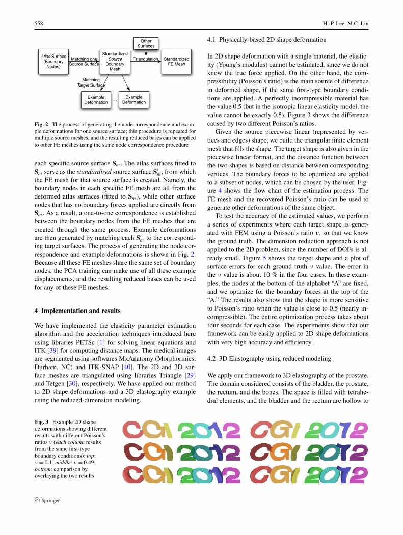
Fig. 2 The process of generating the node correspondence and exam-ple deformations for one source surface; this procedure is repeated formultiple source meshes, and the resulting reduced bases can be appliedto other FE meshes using the same node correspondence procedure

each specific source surface Sm. The atlas surfaces fitted toSm serve as the standardized source surface S′

m, from whichthe FE mesh for that source surface is created. Namely, theboundary nodes in each specific FE mesh are all from thedeformed atlas surfaces (fitted to Sm), while other surfacenodes that has no boundary forces applied are directly fromSm. As a result, a one-to-one correspondence is establishedbetween the boundary nodes from the FE meshes that arecreated through the same process. Example deformationsare then generated by matching each S′

m to the correspond-ing target surfaces. The process of generating the node cor-respondence and example deformations is shown in Fig. 2.Because all these FE meshes share the same set of boundarynodes, the PCA training can make use of all these exampledisplacements, and the resulting reduced bases can be usedfor any of these FE meshes.

4 Implementation and results

We have implemented the elasticity parameter estimationalgorithm and the acceleration techniques introduced hereusing libraries PETSc [1] for solving linear equations andITK [39] for computing distance maps. The medical imagesare segmented using softwares MxAnatomy (Morphormics,Durham, NC) and ITK-SNAP [40]. The 2D and 3D sur-face meshes are triangulated using libraries Triangle [29]and Tetgen [30], respectively. We have applied our methodto 2D shape deformations and a 3D elastography exampleusing the reduced-dimension modeling.

4.1 Physically-based 2D shape deformation

In 2D shape deformation with a single material, the elastic-ity (Young’s modulus) cannot be estimated, since we do notknow the true force applied. On the other hand, the com-pressibility (Poisson’s ratio) is the main source of differencein deformed shape, if the same first-type boundary condi-tions are applied. A perfectly incompressible material hasthe value 0.5 (but in the isotropic linear elasticity model, thevalue cannot be exactly 0.5). Figure 3 shows the differencecaused by two different Poisson’s ratios.

Given the source piecewise linear (represented by ver-tices and edges) shape, we build the triangular finite elementmesh that fills the shape. The target shape is also given in thepiecewise linear format, and the distance function betweenthe two shapes is based on distance between correspondingvertices. The boundary forces to be optimized are appliedto a subset of nodes, which can be chosen by the user. Fig-ure 4 shows the flow chart of the estimation process. TheFE mesh and the recovered Poisson’s ratio can be used togenerate other deformations of the same object.

To test the accuracy of the estimated values, we performa series of experiments where each target shape is gener-ated with FEM using a Poisson’s ratio ν, so that we knowthe ground truth. The dimension reduction approach is notapplied to the 2D problem, since the number of DOFs is al-ready small. Figure 5 shows the target shape and a plot ofsurface errors for each ground truth ν value. The error inthe ν value is about 10 % in the four cases. In these exam-ples, the nodes at the bottom of the alphabet “A” are fixed,and we optimize for the boundary forces at the top of the“A.” The results also show that the shape is more sensitiveto Poisson’s ratio when the value is close to 0.5 (nearly in-compressible). The entire optimization process takes aboutfour seconds for each case. The experiments show that ourframework can be easily applied to 2D shape deformationswith very high accuracy and efficiency.

4.2 3D Elastography using reduced modeling

We apply our framework to 3D elastography of the prostate.The domain considered consists of the bladder, the prostate,the rectum, and the bones. The space is filled with tetrahe-dral elements, and the bladder and the rectum are hollow to

Fig. 3 Example 2D shapedeformations showing differentresults with different Poisson’sratios ν (each column resultsfrom the same first-typeboundary conditions); top:ν = 0.1; middle: ν = 0.49;bottom: comparison byoverlaying the two results

Fast optimization-based elasticity parameter estimation using reduced models 559

Fig. 4 Flow chart of Poisson’s ratio estimation given source and target2D shapes; an FE model is built according to the source shape, and thedistance between the deformed source shape and the target shape isminimized. The red cross marks the nodes with boundary conditionsapplied

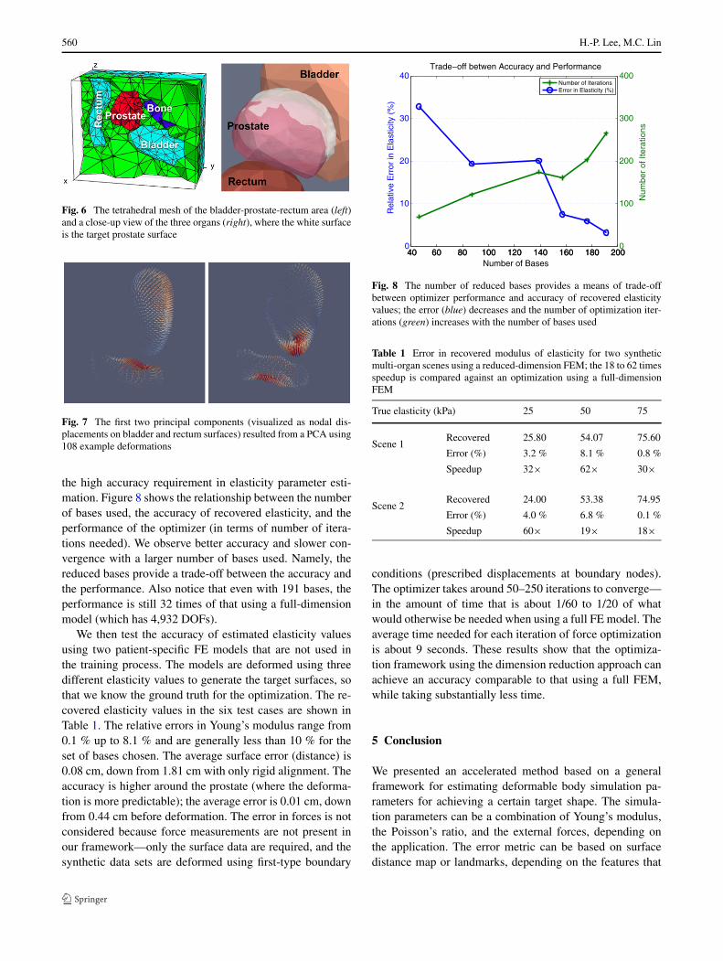
reflect their structure, as shown in Fig. 6. There are two ma-terial properties, one assigned to the prostate (red elementsin Fig. 6), and the other assigned to the elements between or-gans (shown in green in Fig. 6). The goal of the elastographyis to find the ratio of Young’s moduli of the prostate to that ofthe other elements. (The bone is always fixed, so its materialproperty is irrelevant.) The Young’s modulus is the mate-rial property to be optimized here because of its significancein noninvasive cancer detection. Poisson’s ratios are set to0.4 and 0.35 for the two materials, based on common val-ues used in medical simulations [11]. Boundary forces areapplied to the surface nodes of the bladder and the rectum.The parameters to be optimized are the Young’s modulus ofthe prostate and the boundary forces applied to the bladderand the rectum. We have not yet been able to estimate thePoisson’s ratio along with the Young’s modulus because thesurface distance is much less sensitive to the Poisson’s ratio.

Reduced bases training The degrees of freedom for theboundary forces is around 4,900, which makes the optimizerslow to converge (taking thousands of iterations). Therefore,a dimension reduction is performed with 108 example de-formations from CT images. These images are from ninepatient data sets, each has one source image and several tar-get images. The first step of generating examples is to createthe node-to-node correspondence between source surfacesfrom different (patient) data sets. We use a surface matchingapproach to establish the correspondence: an atlas surfaceis iteratively deformed to match each patient-specific sourcesurface, and therefore each patient-specific surface has thesame set of nodes. The patient-specific source surface is thenmatched with corresponding target surfaces to generate theexample deformations for the organ. Figure 7 shows visual-izations (as nodal displacements) of the first two principalcomponents (bases) resulted from the PCA. We choose touse 92 bases for the bladder and 100 for the rectum due to

Fig. 5 Test of accuracy of the recovered Poisson’s ratios ν; the fourtarget shapes are generated using four different ν values; for each sub-figure, on the left is the target shape, and on the right is the plot ofsurface errors versus ν values

560 H.-P. Lee, M.C. Lin

Fig. 6 The tetrahedral mesh of the bladder-prostate-rectum area (left)and a close-up view of the three organs (right), where the white surfaceis the target prostate surface

Fig. 7 The first two principal components (visualized as nodal dis-placements on bladder and rectum surfaces) resulted from a PCA using108 example deformations

the high accuracy requirement in elasticity parameter esti-mation. Figure 8 shows the relationship between the numberof bases used, the accuracy of recovered elasticity, and theperformance of the optimizer (in terms of number of itera-tions needed). We observe better accuracy and slower con-vergence with a larger number of bases used. Namely, thereduced bases provide a trade-off between the accuracy andthe performance. Also notice that even with 191 bases, theperformance is still 32 times of that using a full-dimensionmodel (which has 4,932 DOFs).

We then test the accuracy of estimated elasticity valuesusing two patient-specific FE models that are not used inthe training process. The models are deformed using threedifferent elasticity values to generate the target surfaces, sothat we know the ground truth for the optimization. The re-covered elasticity values in the six test cases are shown inTable 1. The relative errors in Young’s modulus range from0.1 % up to 8.1 % and are generally less than 10 % for theset of bases chosen. The average surface error (distance) is0.08 cm, down from 1.81 cm with only rigid alignment. Theaccuracy is higher around the prostate (where the deforma-tion is more predictable); the average error is 0.01 cm, downfrom 0.44 cm before deformation. The error in forces is notconsidered because force measurements are not present inour framework—only the surface data are required, and thesynthetic data sets are deformed using first-type boundary

Fig. 8 The number of reduced bases provides a means of trade-offbetween optimizer performance and accuracy of recovered elasticityvalues; the error (blue) decreases and the number of optimization iter-ations (green) increases with the number of bases used

Table 1 Error in recovered modulus of elasticity for two syntheticmulti-organ scenes using a reduced-dimension FEM; the 18 to 62 timesspeedup is compared against an optimization using a full-dimensionFEM

True elasticity (kPa) 25 50 75

Scene 1Recovered 25.80 54.07 75.60

Error (%) 3.2 % 8.1 % 0.8 %

Speedup 32× 62× 30×

Scene 2Recovered 24.00 53.38 74.95

Error (%) 4.0 % 6.8 % 0.1 %

Speedup 60× 19× 18×

conditions (prescribed displacements at boundary nodes).The optimizer takes around 50–250 iterations to converge—in the amount of time that is about 1/60 to 1/20 of whatwould otherwise be needed when using a full FE model. Theaverage time needed for each iteration of force optimizationis about 9 seconds. These results show that the optimiza-tion framework using the dimension reduction approach canachieve an accuracy comparable to that using a full FEM,while taking substantially less time.

5 Conclusion

We presented an accelerated method based on a generalframework for estimating deformable body simulation pa-rameters for achieving a certain target shape. The simula-tion parameters can be a combination of Young’s modulus,the Poisson’s ratio, and the external forces, depending onthe application. The error metric can be based on surfacedistance map or landmarks, depending on the features that

Fast optimization-based elasticity parameter estimation using reduced models 561

one can find on the surfaces. The main contribution of ourwork is the acceleration of the optimization framework us-ing reduced-dimension modeling: a set of example defor-mations are used for the statistical training for the bases,which are used to reduce the dimensionality of the parame-ter space. Furthermore, our acceleration method provides atrade-off between performance and accuracy by controllingthe number of bases used. However, the accuracy of the re-duced model is limited by the quantity of example deforma-tions, and therefore our acceleration method is not suitablefor applications lacking examples. We demonstrated thisoptimization-based framework on an implementation usinga linear FEM and reduced-dimension modeling to acceleratethe overall performance by more than an order of magnitude.More complex models, such as the nonlinear FEM, can alsobe used. We have also shown that this method can be easilyapplied to 2D shape deformation and 3D elastography forthe prostate.

In the future, we would like to experiment with differ-ent elasticity models, so that large deformations in charac-ter animations can also be simulated. Since the convergenceof this approach depends on the number of bases needed,the reduced-dimension acceleration technique could benefitfrom a better statistical training method, such as the nonlin-ear PCA. We would also like to integrate the material prop-erty estimation with patient-specific virtual surgery, in orderto provide a more accurate, patient-specific model.

Acknowledgements We thank Mark Foskey, Marc Niethammer,Ron Alterovitz, and Ed Chaney for helpful discussions. We also thankZijie Xu and Dr. Ron Chen for providing prostate patient CT data. Thiswork was partially supported by Army Research Office, National Sci-ence Foundation, and Carolina Development Foundation.

References

1. Balay, S., Gropp, W.D., McInnes, L.C., Smith, B.F.: Efficientmanagement of parallelism in object-oriented numerical soft-ware libraries. In: Modern Software Tools Scientific Computing,pp. 163–202 (1997)

2. Balocco, S., Camara, O., Frangi, A.F.: Towards regional elastogra-phy of intracranial aneurysms. In: Medical Image Computing andComputer-Assisted Intervention, vol. 11, pp. 131–138 (2008)

3. Barbic, J., da Silva, M., Popovic, J.: Deformable object anima-tion using reduced optimal control. ACM Trans. Graph. 28(3), 1(2009). Proceedings of ACM SIGGRAPH 2009

4. Becker, M., Teschner, M.: Robust and efficient estimation of elas-ticity parameters using the linear finite element method. In: Proc.of Simulation and Visualization, pp. 15–28 (2007)

5. Bergou, M., Mathur, S., Wardetzky, M., Grinspun, E.: TRACKS:toward directable thin shells. In: ACM SIGGRAPH 2007 Papers,p. 50 (2007)

6. Bhat, K.S., Twigg, C.D., Hodgins, J.K., Khosla, P.K., Popovic, Z.,Seitz, S.M.: Estimating cloth simulation parameters from video.In: Proceedings of the 2003 ACM SIGGRAPH/EurographicsSymposium on Computer Animation, pp. 37–51 (2003)

7. Bickel, B., Bächer, M., Otaduy, M.A., Lee, H.R., Pfister, H.,Gross, M., Matusik, W.: Design and fabrication of materials withdesired deformation behavior. In: ACM SIGGRAPH 2010 Papers,pp. 1–10 (2010)

8. Bickel, B., Bächer, M., Otaduy, M.A., Matusik, W., Pfister, H.,Gross, M.: Capture and modeling of non-linear heterogeneous softtissue. In: ACM SIGGRAPH 2009 Papers, pp. 1–9 (2009)

9. Cootes, T.F., Taylor, C.J., Cooper, D.H., Graham, J.: Active shapemodels—their training and application. Comput. Vis. Image Un-derst. 61(1), 38–59 (1995)

10. Fu, D., Levinson, S., Gracewski, S., Parker, K.: Non-invasivequantitative reconstruction of tissue elasticity using an iterativeforward approach. Phys. Med. Biol. 45(6), 1495–1510 (2000)

11. Hensel, J.M., Menard, C., Chung, P.W.M., Milosevic, M.F., Kir-ilova, A., Moseley, J.L., Haider, M.A., Brock, K.K.: Developmentof multiorgan finite element-based prostate deformation model en-abling registration of endorectal coil magnetic resonance imagingfor radiotherapy planning. Int. J. Radiat. Oncol. Biol. Phys. 68(5),1522–1528 (2007)

12. Igarashi, T., Moscovich, T., Hughes, J.F.: As-rigid-as-possibleshape manipulation. ACM Trans. Graph. 24(3), 1134–1141(2005)

13. Kallel, F., Bertrand, M.: Tissue elasticity reconstruction using lin-ear perturbation method. IEEE Trans. Med. Imaging 15(3), 299–313 (1996)

14. Kaus, M.R., Brock, K.K., Pekar, V., Dawson, L.A., Nichol, A.M.,Jaffray, D.A.: Assessment of a model-based deformable imageregistration approach for radiation therapy planning. Int. J. Radiat.Oncol. Biol. Phys. 68(2), 572–580 (2007)

15. Krysl, P., Lall, S., Marsden, J.E.: Dimensional model reduction innon-linear finite element dynamics of solids and structures. Int. J.Numer. Methods Eng. 51(4), 479–504 (2001)

16. Lee, H., Foskey, M., Niethammer, M., Lin, M.: Physically-baseddeformable image registration with material property and bound-ary condition estimation. In: Proceedings of the 2010 IEEE In-ternational Conference on Biomedical Imaging: from Nano toMacro, pp. 532–535 (2010)

17. Martin, S., Thomaszewski, B., Grinspun, E., Gross, M.: Example-based elastic materials. In: Proceedings of SIGGRAPH 2011,vol. 30, pp. 72:1–72:8 (2011)

18. McNamara, A., Treuille, A., Popovic, Z., Stam, J.: Fluid controlusing the adjoint method. ACM Trans. Graph. 23(3), 449–456(2004)

19. Müller, M., Gross, M.: Interactive virtual materials. In: Proceed-ings of Graphics Interface 2004, GI’04, pp. 239–246 (2004)

20. Muthupillai, R., Ehman, R.L.: Magnetic resonance elastography.Nat. Med. 2(5), 601–603 (1996)

21. Nealen, A., Muller, M., Keiser, R., Boxerman, E., Carlson, M.:Physically based deformable models in computer graphics. Com-put. Graph. Forum 25, 809–836 (2006)

22. Nocedal, J., Wright, S.: Numerical Optimization. Springer, Berlin(1999)

23. Ophir, J., Alam, S., Garra, B., Kallel, F., Konofagou, E., Krouskop,T., Varghese, T.: Elastography: ultrasonic estimation and imagingof the elastic properties of tissues. Proc. Inst. Mech. Eng., H J.Eng. Med. 213(3), 203–233 (1999)

24. Pai, D.K., Doel, K.v.d., James, D.L., Lang, J., Lloyd, J.E., Rich-mond, J.L., Yau, S.H.: Scanning physical interaction behavior of3D objects. In: Proceedings of SIGGRAPH 2001, SIGGRAPH’01, pp. 87–96 (2001).

25. Pizer, S.M., Fletcher, P.T., Joshi, S., Thall, A., Chen, J.Z., Frid-man, Y., Fritsch, D.S., Gash, A.G., Glotzer, J.M., Jiroutek, M.R.,Lu, C., Muller, K.E., Tracton, G., Yushkevich, P., Chaney, E.L.:Deformable M-Reps for 3D medical image segmentation. Int. J.Comput. Vis. 55(2–3), 85–106 (2003)

26. Press, W.H.: Numerical Recipes. Cambridge University Press,Cambridge (2007)

562 H.-P. Lee, M.C. Lin

27. Rivaz, H., Boctor, E., Foroughi, P., Zellars, R., Fichtinger, G.,Hager, G.: Ultrasound elastography: a dynamic programming ap-proach. IEEE Trans. Med. Imaging 27(10), 1373–1377 (2008)

28. Schnur, D.S., Zabaras, N.: An inverse method for determiningelastic material properties and a material interface. Int. J. Numer.Methods Eng. 33(10), 2039–2057 (1992)

29. Shewchuk, J.R.: Triangle: Engineering a 2D quality mesh gen-erator and Delaunay triangulator. In: Applied Computational Ge-ometry Towards Geometric Engineering, vol. 1148, pp. 203–222.Springer, Berlin (1996)

30. Si, H.: TetGen: a quality tetrahedral mesh generator andthree-dimensional Delaunay triangulator (2009). URL http://tetgen.berlios.de/

31. Skovoroda, A., Emelianov, S.: Tissue elasticity reconstructionbased on ultrasonic displacement and strain images. IEEE Trans.Ultrason. Ferroelectr. Freq. Control 42(4), 141 (1995)

32. Syllebranque, C., Boivin, S.: Estimation of mechanical parametersof deformable solids from videos. Vis. Comput. 24(11), 963–972(2008)

33. Taylor, Z.A., Crozier, S., Ourselin, S.: Real-time surgical simula-tion using reduced order finite element analysis. Med. Image Com-put. Comput. Assist. Interv. 13(Pt 2), 388–395 (2010)

34. Teschner, M., Heidelberger, B., Manocha, D., Govindaraju, N.,Zachmann, G., Kimmerle, S., Mezger, J., Fuhrmann, A.: Colli-sion handling in dynamic simulation environments: the evolutionof graphics: where to nex? In: Eurographics 2005 Tutorial (2005)

35. Treuille, A., McNamara, A., Popovic, Z., Stam, J.: Keyframe con-trol of smoke simulations. In: ACM SIGGRAPH 2003 Papers,pp. 716–723 (2003)

36. Washington, C.W., Miga, M.I.: Modality independent elastogra-phy (MIE): a new approach to elasticity imaging. IEEE Trans.Med. Image 23(9), 1117–1128 (2004)

37. Weng, Y., Xu, W., Wu, Y., Zhou, K., Guo, B.: 2D shape defor-mation using nonlinear least squares optimization. Vis. Comput.22(9–11), 653–660 (2006)

38. Yang, W., Feng, J., Jin, X.: Shape deformation with tunable stiff-ness. Vis. Comput. 24(7–9), 495–503 (2008)

39. Yoo, T.S., Ackerman, M.J., Lorensen, W.E., Schroeder, W., Cha-lana, V., Aylward, S., Metaxas, D., Whitaker, R.: Engineering andalgorithm design for an image processing API: a technical reporton ITK—the insight toolkit (2002)

40. Yushkevich, P.A., Piven, J., Hazlett, H.C., Smith, R.G., Ho, S.,Gee, J.C., Gerig, G.: User-guided 3D active contour segmentation

of anatomical structures: significantly improved efficiency and re-liability. NeuroImage 31(3), 1116–1128 (2006)

41. Zhu, Y., Hall, T., Jiang, J.: A finite-element approach for Young’smodulus reconstruction. IEEE Trans. Med. Imaging 22(7), 890–901 (2003)

42. Zienkiewicz, O.C., Taylor, R.L.: The Finite Element Method, 6thedn. Butterworth-Heinemann, Oxford (2005)

Huai-Ping Lee received B.S. andM.S. degrees in computer sciencefrom National Taiwan Universityand from the University of NorthCarolina at Chapel Hill, respec-tively. He is currently a Ph.D. can-didate at UNC-Chapel Hill. His re-search interests include medical im-age analysis and computer graphics,with focuses on physically-basedmodeling and deformable imageregistration.

Ming C. Lin received the B.S.,M.S., and Ph.D. degrees in electri-cal engineering and computer sci-ence from the University of Califor-nia, Berkeley. She is currently theJohn R. & Louise S. Parker distin-guished professor of computer sci-ence at the University of North Car-olina, Chapel Hill. She has receivedseveral honors and awards, includ-ing IEEE VGTC VR TechnicalAchievement Award 2010 and eightBest Paper Awards. She is a fellowof the ACM and IEEE. Her researchinterests include computer graphics,

geometric computing, robotics, and VR. She has (co)authored morethan 220 refereed publications and coedited/authored four books.