fast numerical simulation of two-phase transport model in the

COMMUNICATIONS IN COMPUTATIONAL PHYSICSVol. 6, No. 1, pp. 49-71

Commun. Comput. Phys.July 2009

Fast Numerical Simulation of Two-Phase Transport

Model in the Cathode of a Polymer Electrolyte Fuel

Cell

Pengtao Sun1,∗, Guangri Xue2, Chaoyang Wang3 and Jinchao Xu2,4

1 Department of Mathematical Sciences, University of Nevada, Las Vegas, 4505Maryland Parkway, Las Vegas, NV 89154, USA.2 Department of Mathematics, The Pennsylvania State University, University Park,PA 16802, USA.3 Departments of Mechanical Engineering and Materials Science and Engineering,Electrochemical Engine Center (ECEC), The Pennsylvania State University,University Park, PA 16802, USA.4 Laboratory of Mathematics and Applied Mathematics, School of MathematicalSciences, Peking University, Beijing 100871, China.

Received 12 December 2007; Accepted (in revised version) 5 July 2008

Available online 13 November 2008

Abstract. In this paper, we apply streamline-diffusion and Galerkin-least-squares fi-nite element methods for 2D steady-state two-phase model in the cathode of polymerelectrolyte fuel cell (PEFC) that contains a gas channel and a gas diffusion layer (GDL).This two-phase PEFC model is typically modeled by a modified Navier-Stokes equa-tion for the mass and momentum, with Darcy’s drag as an additional source term inmomentum for flows through GDL, and a discontinuous and degenerate convection-diffusion equation for water concentration. Based on the mixed finite element methodfor the modified Navier-Stokes equation and standard finite element method for wa-ter equation, we design streamline-diffusion and Galerkin-least-squares to overcomethe dominant convection arising from the gas channel. Meanwhile, we employ Kirch-hoff transformation to deal with the discontinuous and degenerate diffusivity in waterconcentration. Numerical experiments demonstrate that our finite element methods,together with these numerical techniques, are able to get accurate physical solutionswith fast convergence.

AMS subject classifications: 65B99, 65K05, 65K10, 65N12, 65N22, 65N30, 65N55, 65Z05

Key words: Two-phase model, polymer electrolyte fuel cell, Kirchhoff transformation, convectiondominated diffusion problem, streamline diffusion, Galerkin-least-squares.

∗Corresponding author. Email addresses: [email protected] (P. Sun), [email protected] (G. Xue),[email protected] (C. Wang), [email protected] (J. Xu)

http://www.global-sci.com/ 49 c©2009 Global-Science Press

50 P. Sun, G. Xue, C. Wang and J. Xu / Commun. Comput. Phys., 6 (2009), pp. 49-71

1 Introduction

Owing to their high energy efficiency, low pollution, and low noise, fuel cells are widelyregarded as 21st century energy-conversion devices for mobile, stationary, and portablepower. Through tremendous progress made in the past decade, currently available fuelcell materials appear to be adequate for near term markets with highest cost entry points.As a result, industries are currently placing their focus on fuel cell design and engineeringfor better performance, improved durability, cost reduction, and better cold-start charac-teristics. This new focus has led to an urgent need for identification, understanding,prediction, control, and optimization of various transport and electrochemical processesthat occur on disparate length scales in fuel cells.

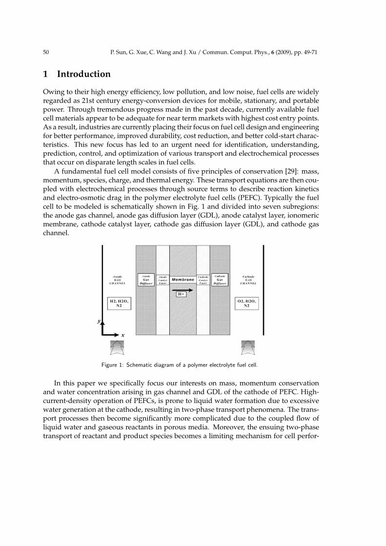
A fundamental fuel cell model consists of five principles of conservation [29]: mass,momentum, species, charge, and thermal energy. These transport equations are then cou-pled with electrochemical processes through source terms to describe reaction kineticsand electro-osmotic drag in the polymer electrolyte fuel cells (PEFC). Typically the fuelcell to be modeled is schematically shown in Fig. 1 and divided into seven subregions:the anode gas channel, anode gas diffusion layer (GDL), anode catalyst layer, ionomericmembrane, cathode catalyst layer, cathode gas diffusion layer (GDL), and cathode gaschannel.

Figure 1: Schematic diagram of a polymer electrolyte fuel cell.

In this paper we specifically focus our interests on mass, momentum conservationand water concentration arising in gas channel and GDL of the cathode of PEFC. High-current-density operation of PEFCs, is prone to liquid water formation due to excessivewater generation at the cathode, resulting in two-phase transport phenomena. The trans-port processes then become significantly more complicated due to the coupled flow ofliquid water and gaseous reactants in porous media. Moreover, the ensuing two-phasetransport of reactant and product species becomes a limiting mechanism for cell perfor-

P. Sun, G. Xue, C. Wang and J. Xu / Commun. Comput. Phys., 6 (2009), pp. 49-71 51

mance, particularly at high current densities, i.e., greater than 1A/cm2. Therefore, a fun-damental understanding of two-phase transport in porous gas diffusion layers of PEFCsis essential in order to improve cell performance.

Wang et al. [32] explored liquid water transport by capillary action, dynamic interac-tion between single- and two-phase zones via evaporation and condensation, and effectsof the phase distribution on gas transport, and described a numerical study of gas-liquid,two-phase flow and transport in the air cathode of PEFC including hydrogen and directmethanol fuel cells. In their models, they employed a modified Navier-Stokes equationto describe the flow in gas channel and GDL simultaneously by adding a Darcy termin the source, so that gas channel is considered as completely permeable, while GDL ispresent as porous media. For water concentration equation, in order to present a unifiedmodel that encompasses both the single- and two-phase regimes, and ensures a smoothtransition between the two, a discontinuous and degenerate function is introduced [32] asdiffusivity of the transport equation in terms of water concentration. In gaseous water re-gion, the water concentration is below a fixed value called saturated water concentration(16mol/m3 at 80C), coinciding with nonzero constant diffusivity. Once water concentra-tion exceeds this fixed value, excess gaseous water is generated and condensed to liquidwater. Correspondingly, the diffusivity suddenly jumps down to zero and then growsup into a smooth functional diffusivity with respect to liquid water concentration. Thusa degenerate and discontinuous diffusivity is induced. On the other hand, both momen-tum equation and concentration equation are all convection-dominated in gas channeldue to the relative large velocity of gas flow.

To deeply investigate the numerical issue of two-phase PEFC models, without lossof generality, we adopt the models introduced by [32] and restrict it in two dimensionalsteady-state case. In this model the most difficult part is how to efficiently deal withthe discontinuous and degenerate diffusivity arising in water concentration equation.Due to significant discontinuity, standard numerical discretization and linearization failin obtaining stable convergent iteration for this nonlinear discontinuous and degeneratetransport equation. The dominant convectional coefficient is another difficulty to getstable convergence for Navier-Stokes equation and convection-diffusion equation in gaschannel.

Therefore, how to accurately and efficiently solve the modified Navier-Stokes equationand discontinuous and degenerate convection-diffusion problem with dominant convec-tion terms are the fundamental numerical issues for two-phase transport model in thecathode of polymer electrolyte fuel cell, which is also the main goal of this paper.

The rest of this paper is organized as follows. First of all, the governing equationsfor two-phase steady-state transport problem in both gas channel and GDL are definedin Section 2. In Section 3, we introduce the method of Kirchhoff transformation [1, 2,5, 7, 18, 33] and address how efficiently it deals with the discontinuous and degeneratediffusivity. The entire finite element discretizations is given in Section 4, where a typeof mixed finite element method is employed to discretize momentum and continuityequations, and Kirchhoff transformation is adopted to solve the discontinuous and de-


generate water concentration equation. The dominant convection terms are dealt withby means of streamline-diffusion scheme [11, 12, 14, 17, 20] and Galerkin-least-squaresscheme [8, 9, 25, 26]. Numerical simulations of several practical cases are illustrated inSection 5, indicating that our numerical schemes significantly improve the computationalperformance in efficiency as well as accuracy.

2 The 2D steady-state two-phase transport model in PEFC

cathode

Based on [15], in this section we describe the governing equations for 2D steady-statetwo-phase transport problem in the cathode of PEFC, define the relevant physical pa-rameters and coefficients, as well as their boundary conditions. All of the involved pa-rameters refer to Table 1 in Section 2.2.

2.1 Governing equations

Specifically for 2D steady-state two-phase transport model in both gas channel and GDL,we introduce its governing equations in twofold fields: flow and species concentration.

Flow equations. For flow field with velocity ~u and pressure P as unknowns, we havethe following modified Navier-Stokes equations

1

ε2∇·(ρ~u~u)=∇·(µ∇~u)−∇P+Su, (2.1a)

∇·(ρ~u)=0, (2.1b)

where ε is porosity of air cathode, ρ is density, µ is effective viscosity. We know (2.1b)is exact continuity equation, and (2.1a) represents a modified momentum equation, inwhich we indicate that the additional source term Su is named as Darcy’s drag and de-fined as follows

Su =−µ

K~u, (2.2)

where K is a position-dependent ”permeability” in porous cathode, defined as

K =

+∞ in gas channel,KGDL =10−12 in GDL.

(2.3)

The definition of K implies that gas channel is considered as completely permeable, whileGDL is present as porous media with small permeability KGDL.

Darcy’s drag Su is exactly developed from Darcy’s Law in porous GDL:

~u=−KGDL

µ∇P.


When K=∞ in gas channel, Su =0 according to (2.2). Therefore (2.1a) reduces to classicalmomentum equation. On the other hand, notice that permeability KGDL = 10−12 andε = 0.3 in GDL, all the rest terms in (2.1a) in GDL become negligible after multiplyingpermeability K on both sides, which induces (2.1a) to tend to be Darcy’s law along with arescaled gradient pressure vector.

By virtue of this additional source term Su, the momentum balance equation is mod-ified to be valid in both GDL and gas channel, presenting the extended Darcy’s law fortwo-phase flow in porous GDL with small permeability, and exact Navier-Stokes equa-tion in gas channel with unit porosity and infinite permeability. (2.1) is also known asDarcy-Brinkman-Forchheimer model [13], which is typically used to model the flow insidethe porous domain. Finite difference method was first employed in [6] for such modelinvolving the Navier-Stokes equations with an added Darcy term. Then a uniformly sta-ble finite element method was developed in [34] with respect to the singularly perturbedcoefficients for similar model.

The advantage of modified Navier-Stokes equation (2.1) is that, we simultaneouslysolve Darcy-Navier-Stokes flow in one single domain, instead of two-domain approachwhere Beavers-Joseph-Saffman interface condition [4, 10, 19] along the tangential directionof GDL/gas channel interface, continuity of mass flux and continuity of normal stressacross GDL/gas channel interface must be employed. The equivalence between thesetwo approaches is discussed in [21]. Obviously single domain approach is easier toimplement, especially in the simulation of three dimensional complete fuel cell model,which will be investigated in separate paper [23].

Species concentration equation. Water management is one of the key issues in poly-mer electrolyte fuel cell. Due to the coexistence of single phase zone and two phase zone,water equation turns to be the most important and difficult species equation to deal withthrough the entire fuel cell. Therefore, for species concentration equations, in order tofocus on water management topics, without loss of generality, we typically consider sin-gle component model by taking water as the only species in the simplified concentrationequation.

Water concentration equations are spatially defined as follows with respect to waterconcentration C [15]

∇·(γc~uC)=∇·(Γ(C)∇C), in GDL; (2.4a)

∇·(~uC)=∇·(De f fg ∇C), in gas channel, (2.4b)

where γc is the advection correction factor defined in Section 2.2, the diffusivity Γ(C) inGDL is defined as

Γ(C)=

Γcapdi f f , if C≥Csat;

De f fg , if C<Csat.

(2.5)

Here Csat is saturated water concentration. De f fg = ε1.5Dgas is the effective water vapor

diffusivity, namely, the constant diffusivity in gaseous water region. Γcapdi f f is capillary


diffusion coefficient, i.e. the functional diffusivity in liquid water region, defined as fol-lows in terms of liquid saturation s:

Γcapdi f f =

∣∣∣∣(mfl

M−

Csat

ρg)(

M

ρl−CsatM)

λlλg

νσcosθc(εK)1/2 dJ(s)

ds

∣∣∣∣, (2.6)

here s∈ [0,1] denotes the liquid saturation throughout the paper. It is a basic variable inmultiphase mixture (M2) model [31, 32], and has coequality with water concentration as

C=ρls

M+Csat(1−s),

hences=(C−Csat)/(

ρl

M−Csat).

J(s) is the Leverett function, given by

J(s)=

1.417(1−s)−2.120(1−s)2 +1.263(1−s)3, if θc <90;1.417s−2.120s2 +1.263s3, if θc >90.

According to the definitions of physical parameters and coefficients in Section 2.2, wecan easily calculate that Γcapdi f f =0 when C=Csat or s=0. So Γcapdi f f , and further Γ(C), isdegenerate at Csat.

The behavior of diffusivity Γ(C) can be better understood in Fig. 2, where Γ(C) isclearly indicated as a discontinuous and degenerate function with respect to C. Csat =16 mol/m3 is the typical point at which discontinuity and degeneracy occur for Γ(C) atthe same time.

Figure 2: Γ(C).

When the gas channel is dry, although there is huge jump in diffusivity Γ(C) betweenthe single- and two-phase regimes in GDL, Γ(C) is still continuous across the GDL/gas

channel interface due to the same constant diffusivity De f fg .

Governing equations (2.1) and (2.4), together with the definitions of physical coeffi-cients and parameters in Section 2.2 and the boundary conditions in Section 2.3, consti-tute the 2D steady-state two-phase transport model in the cathode of polymer electrolytefuel cell.


2.2 Coefficients and parameters

The physical coefficients and mixture variables arising in the governing equations (2.1),(2.4) and the definitions of their coefficients are specifically defined for single componenttwo-phase transport PEFC model as follows:

• Density ρ=ρls+ρg(1−s),

• Relative mobilities λl(s)= krl/νl/(krl/νl +krl/νg) and λg(s)=1−λl(s),

• Relative permeabilities krl = s3 and krg =(1−s)3,

• Kinematic viscosity ν=(krl/νl +krg/νg)−1,

• Effective viscosity µ=(ρl ·s+ρg ·(1−s)/(krl/νl +krg/νg),

• Advection correction factor γc = (ρ(λlmfl +λgmfg))/(ρlmfls+ρgmfg(1−s)),where mfl =1,mfg =CsatM/ρg are mass fractions of liquid water and gaseouswater, respectively.

Advection correction factor γc is a continuous function with respect to concentration.In gas channel we always assume water closes to be gaseous phase, i.e., s=0. Therefore,γc is correspondingly reduced to be unity and the continuity of convectional coefficientsof (2.4) are then preserved while crossing over the GDL/gas channel interface.

Other property parameters refer to Table 1.

Table 1: Property parameters.

Parameter Symbol Value Unit

Water vapor diffusivity Dgas 2.6×10−5 m2/sWater molecular weight M 0.018 kg/molVapor density ρg 0.882 kg/m3

Liquid water density ρl 971.8 kg/m3

Surface tension σ 0.0625 kg/s2

Contact angle between two phases θc23 π

Porosity of GDL ε 0.3Kinematic liquid water viscosity νl 3.533×10−7 m2/sKinematic vapor viscosity νg 3.59×10−5 m2/sFaraday constant F 96487 A·s/molCurrent density at the left end I1 20000 A/m2

Current density at the right end I2 10000 A/m2

One advantage of multiphase mixture (M2) model [30–32] is that we do not need totrack phase interfaces between single- and two-phase regimes, it is automatically indi-cated by the solution, and therefore greatly simplifies numerical simulation of currenttwo-phase transport problem. In fact, according to above definitions of coefficients, all


the governing equations (2.1), (2.4) identically reduce to their single-phase counterpartsin the limits of the liquid saturation, s, equals to zero and unity, respectively.

2.3 Computational domain and boundary conditions

We specifically consider that governing equations (2.1) and (2.4) take place in the cathodeof PEFC which consists of gas diffusion layer and opening gas channel, as schematicallyshown in Fig. 3. The horizontal x-axis represents the flow direction and the vertical y-axis points in the through-plane direction. The geometric sizes of this computationaldomain are marked in Fig. 3 as well, where the physical width of GDL and gas channelare δGDL =3×10−4 m, δCH =10−3 m, respectively, in comparison with the length in flowdirection lPEFC =7×10−2 m. The large aspect ratio of the channel length to width, whichis up to about 1 :100, exhibits a very micro-fabricated thin-film structure.

Figure 3: Domain.

At the inlet of the gas channel ((∂Ω)1 in Fig. 3), constant flow rate and water con-centration are specified. At the outlet ((∂Ω)3 in Fig. 3), both velocity and concentrationfields are assumed to be fully developed. Hence based on this computational domain,the boundary conditions are indicated as follows.

For flow field equation (2.1), the following boundary conditions hold with respect tovelocity ~u:

u1 =u1|inlet(m/s),u2 =0 at inlet (∂Ω)1,

where u1|inlet are given in (4.8);

(P−µ∇~u)·~n=0 at outlet (∂Ω)3;

~u=0 at the bottom wall (∂Ω)5; ~u=0 at side and top walls (∂Ω)2,(∂Ω)4 and (∂Ω)6.

For water concentration (2.4), the following boundary conditions hold with respect toconcentration C: at channel inlet (∂Ω)1, C = Cin(mol/m3); at the bottom and side walls


(∂Ω)2,(∂Ω)3,(∂Ω)4 and channel outlet (∂Ω)5, ∇C ·~n=0; at the top wall (∂Ω)6, the liquidwater mass flux condition is given by:

Γ(C)∇C ·~n−γc~uC ·~n=I(x)

2F, (2.7)

where the Dirichlet boundary condition at (∂Ω)1 is usually set as Cin<Csat to indicate theinput of gaseous component. At the membrane/cathode surface ((∂Ω)6), the nonhomo-geneous Neumann boundary condition is given to simulate oxygen reduction reactionoccurring in catalyst layer and generating liquid water mass flux, which is demonstratedby Faraday’s law as shown in the right hand side of (2.7) [29], where I(x) is the volumetrictransfer current of the reaction (or transfer current density) defined by a linear functionas follows

I(x)=

(I1−(I1− I2)

x

lPEFC

)[A

m2

], (2.8)

where I1, I2 are technically given in Table 1. (2.8) is the linear reduction of Butler-Volmerequation, indicates that the transfer current density linearly decreases from constant localcurrent density I1 at left end of membrane/cathode interface (top wall) to I2 at right end.This is an approximation of transfer current density for our simplified single componenttwo-phase PEFC model due to the absence of electric potentials.

3 Kirchhoff transformation

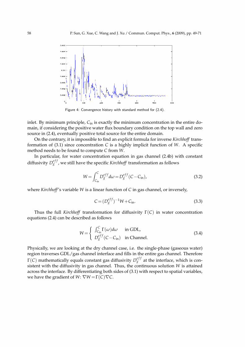
In this section, we start our numerical efforts with water concentration equation (2.4)first. Due to highly nonlinear discontinuous and degenerate diffusivity Γ(C) defined in(2.5), it is hard to obtain convergent solution for the nonlinear iteration of (2.4) with stan-dard finite element discretization. This nonconvergent phenomenon has been revealedby many numerical experiments with finite-volume based commercial flow solvers andour in-house code of standard finite element method [22], as shown in Fig. 4. Therefore,an efficient discretization scheme to deal with the nonlinear discontinuous and degen-erate diffusivity Γ(C) is the key to make the entire nonlinear iteration converge fast. Tothis end, by Kirchhoff transformation technique [1,2,5,7,18,33], we are able to reformulate(2.4) to a semilinear convection diffusion equation with simple Laplacian term as diffusionwith respect to a new variable, where the nonlinearity, discontinuity and degeneracy aris-ing in diffusivity Γ(C) all disappear. Instead, we need to implicitly solve inverse Kirchhofftransformation in order to obtain the desired concentration.

First of all, based on diffusivity Γ(C), we define a new variable W in terms of Kirchhofftransformation

W(C)=∫ C

Cmin

Γ(ω)dω. (3.1)

Hence W is a function of concentration C≥Cmin, where Cmin is the lower bound of con-centration. Here we can take Cmin =Cin, the entry concentration of gaseous water on the


Figure 4: Convergence history with standard method for (2.4).

inlet. By minimum principle, Cin is exactly the minimum concentration in the entire do-main, if considering the positive water flux boundary condition on the top wall and zerosource in (2.4), eventually positive total source for the entire domain.

On the contrary, it is impossible to find an explicit formula for inverse Kirchhoff trans-formation of (3.1) since concentration C is a highly implicit function of W. A specificmethod needs to be found to compute C from W.

In particular, for water concentration equation in gas channel (2.4b) with constant

diffusivity De f fg , we still have the specific Kirchhoff transformation as follows

W =∫ C

Cin

De f fg dω = D

e f fg (C−Cin), (3.2)

where Kirchhoff ’s variable W is a linear function of C in gas channel, or inversely,

C=(De f fg )−1W+Cin. (3.3)

Thus the full Kirchhoff transformation for diffusivity Γ(C) in water concentrationequations (2.4) can be described as follows

W =

∫ CCin

Γ(ω)dω in GDL,

De f fg (C−Cin) in Channel.

(3.4)

Physically, we are looking at the dry channel case, i.e. the single-phase (gaseous water)region traverses GDL/gas channel interface and fills in the entire gas channel. Therefore

Γ(C) mathematically equals constant gas diffusivity De f fg at the interface, which is con-

sistent with the diffusivity in gas channel. Thus, the continuous solution W is attainedacross the interface. By differentiating both sides of (3.1) with respect to spatial variables,we have the gradient of W: ∇W =Γ(C)∇C.


By virtue of (3.4), and considering continuity equation (2.1b) in gas channel, we canreformulate (2.4) to an equivalent new water concentration equation with respect to W,along with new corresponding boundary conditions as follows

∆W =∇·(γc~uC) in GDL, (3.5a)

∆W =∇·((De f fg )−1

~uW) in gas channel, (3.5b)

W =0 on (∂Ω)1, (3.5c)

∂W

∂n−γc~uC ·~n=

I

2Fon (∂Ω)6, (3.5d)

∂W

∂n=0 elsewhere on ∂Ω. (3.5e)

We observe that only one single Laplacian term is involved in the left hand side of(3.5a) and (3.5b), the original discontinuous and degenerate diffusivity Γ(C) has beenhidden inside the Kirchhoff transformation (3.1), which significantly reduces the difficultyof nonlinear iteration and makes fast convergence imaginable. Now the only nonlinear-ity stays in the right hand side of (3.5a), the convection term ∇·(γc~uC(W)), where C isan implicit function of W in terms of the inverse Kirchhoff transformation and the nonlin-earity is introduced.

We notice that the convection term in GDL quite differs from that in gas channel. Wereformulate them in different ways because of the significant distinction they bear onthe convectional coefficients. On account of the linear inverse Kirchhoff transformation(3.3) in gas channel, we can directly get linear convectional coefficient for W in (3.5b).But the inverse Kirchhoff transformation in GDL is implicitly given, no explicit formulato change variable C to W directly. On the other hand, it is hazardous if we insist onapplying Kirchhoff transformation to ∇·(γc~uC), a new convection term that explicitlydepends on W will be obtained as

∇·(γc~uC)=γc~u·∇C+∇·(γc~u)C=γc~u·∇W

Γ(C)+∇·(γc~u)C(W).

As a result, a large or even infinite convection term ∇W/Γ(C) may be produced whenC is close to the degenerate point Csat and then Γ(C) approaches zero. Therefore wemust avoid applying Kirchhoff transformation to the convection term in (3.5a). Thanksto relatively very small Darcy’s velocity ~u in GDL in comparison with flow velocity inopening gas channel, this convection term is not dominant at all, accordingly we are ableto keep its original form unchanged and move it to the right hand side as equivalentsource term. This additional source term does not explicitly depend on W, which allowus to directly compute it by updating C from the latest W in terms of a doable inverseKirchhoff transformation of (3.1).

Actually (3.5a) is only a semilinear equation because there is one single C stays in theright hand side which depends on W via the inverse Kirchhoff transformation, an implicitfunction. Picard’s method is sufficient to linearize it. In each iteration step, C is updated


by the inverse Kirchhoff transformation from W. In contrast to (3.5a), (3.5b) is just a linearequation in gas channel, velocity ~u is remarkably large therein, which results in domi-nant convection term in (3.5b). So we cannot consider the preformation of convection

term ∇·((De f fg )−1~uW) as an additional source term. It has to be reformulated to cur-

rent explicit convection form of W via linear Kirchhoff transformation (3.3) and treated bycertain upwind scheme in its discretization in order to stabilize the numerical solution.

In view of the weak nonlinearity in (3.5), we would be able to expect fast convergenceof nonlinear iteration for W, and consequently for C, if an accurate and efficient methodcould carry the inverse Kirchhoff transformation of (3.1) into effect. It is nontrivial tocompute this inverse Kirchhoff transformation directly [27, 28]. One relatively simple ap-proach is Look-Up Table (LUT) method, namely, search corresponding value of C in asorted relational data table between W and C at certain value of W by one data searchmethod, say, bisection. For more accurate and faster approach, see [24] where we presenta type of Newton’s method to efficiently deal with the inverse Kirchhoff transformation.

4 Finite element approximations

In this section we design our finite element discretizations for Navier-Stokes equation (2.1)and the reformulated water concentration equation (3.5). Considering their various non-linearities, we particularly employ Newton’s method to linearize the nonlinear convectionterm in (2.1) and Picard’s scheme to linearize the nonlinear source term in (3.5).

4.1 Newton’s linearization for Navier-Stokes equation (2.1)

Before Newton’s linearization, we rewrite (2.1) as following equivalent forms by applyingcontinuity equation (2.1b) to the convection term in momentum equation (2.1a), and thensplitting continuity equation to two parts in order to constitute a saddle point system:

ρ

ε2~u·∇~u=∇·(µ∇~u)−∇P−

µ

K~u, (4.1a)

∇·~u=−∇ρ

ρ·~u, (4.1b)

Newton’s linearization for (4.1) follows thereafter. Provided (~un,Cn) are given, we define(~un+1,Pn+1) as the iterative solutions of the following Newton’s linearization scheme (n=0,1,2,···):

ρn

ε2(~un ·∇~un+1+∇~un ·~un+1)

=∇·(µn∇~un+1)−∇Pn+1−µn

K~un+1+

ρn

ε2~un ·∇~un, (4.2a)

∇·~un+1 =−∇ρn

ρn·~un. (4.2b)


If the above scheme converges, then we can pass the limit n→∞ on both sides of (4.2).Since ~un→~u,ρn→ρ,µn →µ, the limit of (4.2) is eventually equivalent to (4.1), the validityof linearization scheme (4.2) is confirmed.

4.2 Picard’s linearization for concentration equation (3.5)

Given (~un,Cn), we define (Wn+1,Cn+1) as the iterative solution of the following Picard’slinearization scheme (n=0,1,2,···):

∆Wn+1 =∇·(γc~u

nCn) in GDL,

∆Wn+1 =∇·((De f fg )−1~unWn+1) in gas channel,

(4.3)

together with the inverse Kirchhoff transformation, we obtain Cn+1 from Wn+1.

4.3 Weak forms

We define

V :=~v=(v1,v2)⊤∈ [H1]2

∣∣v1|(∂Ω)1=u1|inlet,

Q :=w∈H1∣∣w|(∂Ω)1

=0, P := L2,

V :=~v=(v1,v2)⊤∈ [H1]2

∣∣v1|(∂Ω)1=0.

Then the mixed weak forms of (4.1) and (3.5) on the basis of linearizations (4.2) and (4.3)are presented as follows: for any (~v,q,w)∈ V×P×Q, find (~un+1,Pn+1,Wn+1)∈V×P×Q,such that

(µn∇~un+1,∇~v)+(ρn

ε2~un ·∇~un+1,~v)+(

ρn

ε2∇~un ·~un+1,~v)

−(Pn+1,∇·~v+(µn

K~un+1,~v)=(

ρn

ε2~un ·∇~un,~v), (4.4a)

−(∇·~un+1,q)=(∇ρn

ρn·~un,q), (4.4b)

(∇Wn+1,∇w)=(γc~unCn,∇w)+

∫

(∂Ω)6

I(x)

2Fwdx in GDL, (4.4c)

(∇Wn+1,∇w)−((De f fg )−1

~unWn+1,∇w)

+∫

(∂Ω)3

(De f fg )−1

~un ·~nWn+1wdy=0 in gas channel. (4.4d)

4.4 Finite element discretization

In correspondence with mixed weak forms (4.4), we employ mixed finite element methodto discretize Navier-Stokes equations (4.1), and apply standard finite element method to


reformulated water concentration equation (3.5) as well. Considering the convectionterm in (4.1a) and (3.5b) could be dominant due to the large velocity ~u in gas channel,therefore, in order to stabilize the numerical computation for nonlinear iteration (4.2) and(4.3), we need certain upwind scheme to overcome these possibly dominant convectionterms.

Since finite-difference based upwind scheme cannot directly work for finite elementdiscretization, as substitutes, streamline-diffusion scheme [11, 12, 14, 17, 20] and Galerkin-least-squares scheme [8,26] are appropriately chosen to deal with dominant convectionalcoefficients in the framework of finite element method. Typically, we apply Galerkin-least-squares scheme to (4.1a) and streamline-diffusion scheme to (3.5b), respectively, dueto their own specific convective features. In our another paper [24], we will discuss acombined finite element-upwind finite volume method for this nonlinear convection-diffusion problem by employing a finite-volume based upwind scheme to specificallydeal with dominant convection term only.

To discretize weak forms (4.4) via finite element method in the domain shown inFig. 3, we firstly define the finite element space Sh=Vh×Ph×Qh⊂V×P×Q on certain uni-form or quasi-uniform triangulation Th, where Vh consists of piecewise quadratic polyno-mials, and Ph and Qh consist of piecewise linear polynomials, h represents the maximummesh size. In Sh, subspace Vh×Ph is exactly the well known space of Taylor-Hood el-ement, one type of stable mixed finite element specifically for saddle-point variationalproblem [3]. The purpose of such choice for finite element space Sh is to approximatevelocity with quadratic element (P2), and pressure and concentration with linear element(P1), simultaneously, on the theoretical basis of Babuska-Brezzi-Ladyzhenskaya condition(BBL) and its discrete form [16].

Based on weak forms (4.4), we define the following mixed finite element discretiza-tion, combining with Galerkin-least-squares and streamline-diffusion schemes togetherto deal with the dominant convection terms in momentum equation and concentrationequation, respectively.

For any given (~v,q,w)∈Sh, find (~un+1h ,Pn+1

h ,Wn+1h )∈Sh (n=0,1,2,···), such that

((µ(Cnh )∇~un+1

h ,∇~v)+(ρ(Cn

h )

ε2~un

h ·∇~un+1h ,~v)

+(ρ(Cn

h )

ε2∇~un

h ·~un+1h ,~v)−(Pn+1

h ,∇·~v)+(µ(Cn

h )

K~un+1

h ,~v)

+δgls(h)·(L(~un+1

h ,Pn+1h ,Wn+1

h ),L(~v,q,w))

=(ρ(Cn

h )

ε2~un

h ·∇~unh ,~v), (4.5a)

−(∇·~un+1h ,q)=(

∇ρ(Cnh )

ρ(Cnh )

·~unh ,q), (4.5b)

(∇Wn+1h ,∇w)=(γc~u

nhCn

h ,∇w)+∫

(∂Ω)6

I(x)

2Fwdx (GDL), (4.5c)


(∇Wn+1h ,∇w)−((D

e f fg )−1

~unhWn+1

h ,∇w)+∫

(∂Ω)3

(De f fg )−1

~unh ·~nWn+1

h wdy

+δsld(h)((D

e f fg )−1

~unh ·∇Wn+1

h ,(De f fg )−1

~unh ·∇w

)

−δsld(h)

((D

e f fg )−1∇ρ(Cn

h )

ρ(Cnh )

·~unhWn+1

h ,(De f fg )−1

~unh ·∇w

)=0 (Gas channel), (4.5d)

where the last term in the left hand side of (4.5a) is a stabilizing term, derived fromGalerkin-least-squares scheme in terms of L, which is the momentum operator of (4.1)and defined as

L(~u,P,W)=−∇·(µ(C(W))∇~u)+ρ(C(W))

ε2~u·∇~u+∇P+

µ(C(W))

K~u.

This stabilizing term added is obtained by minimizing the sum of the squared residual ofthe momentum equation integrated over each element domain. It involves the momen-tum equation as a factor, therefore, despite this additional term, an exact solution is stilladmissible to the variational formulation given by (4.4).

Similarly, the streamline-diffusion scheme introduces the last term in the left handside of (4.5d). Both of these two schemes aim at balancing the magnitudes between dom-inant convection term and insignificant diffusion term by working together with twoimportant parameters δgls(h) and δsld(h). Although they present different forms, bothof them intend to introduce artificial diffusivity (viscosity) into the discretization. Toexecute this mission, besides the additional discrete diffusive forms as shown above, pa-rameters δgls(h) and δsld(h) play another important role here. Basically they hold

δgls(h)=Cglsh, δsld(h)=Csldh,

i.e., δgls(h) and δsld(h) are proportional to mesh size h, Cgls and Csld are certain constantparameters. Therefore, when mesh size h is sufficiently small, the additional diffusiveterms introduced by Galerkin-least-squares and streamline-diffusion schemes eventuallyapproximate to zero with the rate of convergence O(h). So numerical discretization (4.5)still approaches the original one when h is small enough.

In practice, it is difficult to give a generic formula for Cgls and Csld in nonlinear case[11, 12, 14, 17, 20]. They have to be chosen artificially in order to obtain the optimal stablesolutions. Usually starting with small ones, we gradually increase the values of Cgls andCsld and compute the corresponding finite element equations (4.5) until gained numericalsolutions are not oscillating any more in convection-dominated opening gas channel.

We state the algorithm of implementing finite element discretizations (4.5) in Algo-rithm 4.1.

In Algorithm 4.1, we need to indicate the initial guesses (~u0h,C0

h). Although there is nocertain way to define the initial guess, in practice, usually it can be simply given in termsof boundary conditions and physical phenomena. It is well known that the flow profileis parabolic once laminar flow is fully developed in long, straight channel, under steady


Algorithm 4.1:

For n≥0, given ~u0h,C0

h, the following procedures are successively executed:

1. Implicitly solve (4.5) for (~un+1h ,Pn+1

h ,Wn+1h ) first.

2. Calculate Cn+1h with Wn+1

h in terms of the inverse Kirchhoff transformation.

3. Determine if the following stopping criteria hold:

‖~un+1h −~un

h‖L2(Ω)+‖Pn+1h −Pn

h ‖L2(Ω)+‖Cn+1h −Cn

h‖L2(Ω)

‖~unh‖L2(Ω)+‖Pn

h ‖L2(Ω)+‖Cnh‖L2(Ω)

< tolerance, (4.6)

which is the relative convergence error in successive two iteration steps. If yes, then numericalsimulation is done. Otherwise, go back to the first step and continue.

flow conditions. Based on this fact, we are able to assign the initial data of velocity asfollows

(u0h)1 =

uinsin(yπ/δCH), x=0, 0≤y≤δCH (inlet),

0, elsewhere,

(u0h)2 =0, C0

h =Cin,

(4.7)

where (u0h)1 is the x-component of ~u0

h. We use a sin function to approximate (u0h)1 as a

parabolic-like function at the inlet, an approximation of laminar flow in long, straightgas channel, whose the highest velocity uin (m/s) occurs at the center of inlet (y=δCH/2)and quadratically decays to zero on the boundary wall. This initial guess is close tothe real case of parabolic flow in relative long gas channel. It would be helpful to attaingood convergence for nonlinear iteration accordingly. As a consequence, in the followingnumerical experiments, we assign the Dirichlet boundary condition of velocity at the inletas follows

u1|inlet =uinsin(yπ/δCH), 0≤y≤δCH. (4.8)

Considering Kirchhoff transformation (3.1) does not depend on the spatial domainbut only concentration variable, we can directly generalize it to three dimensional case.Consequently numerical discretizations (4.5) are also able to be equivalently extended tothree dimensional PEFC model without any difficulty.

In Section 5, a dry inlet will be chosen as a case of study therein because of recentinterests in proton exchange membrane fuel cells (PEMFC) without external humidifica-tion and low-humidity, self-sustaining fuel cells for portable electronics. In addition, thedry inlet of the air cathode is of potential relevance to direct methanol fuel cell (DMFC).Thus the entire numerical methods studied in this section can be applied to this dry caseimmediately.


5 Numerical simulations

In practice, the magnitudes of imported velocity and concentration at the inlet of gaschannel produce dramatic affection to velocity and water concentration field in bothgas channel and GDL. Smaller concentration (Cin <Csat) and bigger entry velocity (uin ≥3m/s), which imply dry air and fast vapor transport rate, may have greater possibilityto keep gas channel dry than the other way round. On the other hand, higher transfercurrent density I makes cathode reaction require more oxygen and generate more liquidwater at membrane/cathode surface, which increases the amount of liquid water presentin GDL and clearly forms the two-phase region. When accumulated liquid water in GDLdrives the interface of single- and two-phase regions reaches over GDL/gas channel in-terface, wetted gas channel is produced accordingly.

In this section, we will illustrate these physical phenomena with the numerical meth-ods mentioned in Section 4 by imposing various physical entry velocities at the inlet andtransfer current densities I at membrane/cathode surface (∂Ω)6. Simultaneously the ef-ficiency and accuracy of our presented numerical techniques are exhibited.

First of all, we define the triangulation Th on the domain shown in Fig. 3 with 20intervals for the length of fuel cell along x-direction, 30 and 25 intervals for the widthof gas channel and GDL, respectively, along y-direction. So the number of total grids inTh is 20×(30+25) = 1100. The tolerance of our stopping criteria (4.6) for the nonlineariteration is 10−10.

Figure 5: Convergence histories (left) FEM with Kirchhoff transformation; (right) standard FEM withoutKirchhoff transformation.

Case 1: Cin=14 mol/m3, uin=3 m/s, average current density I=1.5Acm−2. Providedthat a practical boundary condition Cin=14mol/m3,uin=3m/s is reinforced at the inlet ofgas channel, and liquid water mass flux condition (2.7) is assigned at membrane/cathodesurface with the average cell current density (I1+ I2)/2=1.5Acm−2, we gain reasonablephysical solutions by employing numerical discretization (4.5) and appropriately choos-


Figure 6: Horizontal two-phase mixture velocity in thecase of Cin =14mol/m3,uin =3m/s, I =1.5Acm−2.

Figure 7: Vertical two-phase mixture velocity in thecase of Cin =14mol/m3,uin =3m/s, I =1.5Acm−2.

Figure 8: Two-phase mixture velocity field in the case of Cin =14mol/m3,uin =3m/s, I =1.5Acm−2.

ing parameters Cgls and Csld for nearly optimal control on dominant convectional coeffi-cients. These results are quite similar with [32], see Figs. 6-12 within only 19 nonlineariteration steps. Fig. 5 displays the fast convergence process with Kirchhoff transformationand oscillating iteration without Kirchhoff transformation, respectively.

In the following, the focus is placed on elucidating numerical simulation results shownin Figs. 6-12, where the interface of gas channel and GDL is indicated in these figures bya bold line.

Figs. 6-8 shows the velocity field of the two-phase mixture in the GDL and gas chan-nel. As expected, there is a large difference in the velocity scale between the porousGDL and the open channel. The mixture velocity in porous GDL is at least two ordersof magnitude smaller than that in the open gas channel, indicating that gas diffusion isthe dominant transport mechanism in porous GDL. The flow field in the open channel isfully developed in view of the large aspect ratio of the channel length to width, as can beseen in Fig. 8 where the channel length is, however, not drown to scale for better view.

Fig. 10 displays the water concentration distribution whose value is below Csat, pre-senting in the phase of water vapor, in the porous cathode and flow channel. As the airflows down the channel, water vapor is continuously added from the cathode, resultingin an increased water vapor concentration along the channel. As a result, liquid wa-ter may first appear in the vicinity of the membrane/cathode interface near the channeloutlet. A two-phase zone at this location is indeed predicted in the present simulationshown in Fig. 9, where the water concentration is greater than Csat, and water vapor iscondensed into liquid water therein.


Figure 9: Concentration in the case of Cin =14mol/m3,uin =3m/s, I =1.5Acm−2.

Figure 10: Water vapor concentration in the case ofCin =14mol/m3,uin =3m/s, I =1.5Acm−2.

Figure 11: Liquid water saturation in the case of Cin=14mol/m3,uin=3m/s, I=1.5Acm−2. The evaporationfront separating the two-phase zone from the single-phase region is approximately represented by s=0.01.

Figure 12: Kirchhoff ’s variable W in the case of Cin=14mol/m3,uin =3m/s, I =1.5Acm−2.

In accordance with Fig. 9, liquid water is seen in the upper-right corner of Fig. 11 tocoexist with the saturated water vapor. The largest liquid amount predicted in Fig. 11 isaround 6.8% at the average current density of 1.5 A cm−2, matching well with 6.3% atthe current density of 1.4 A cm−2 in [32] where a full PEFC model is considered and thecurrent density I is exactly computed in terms of Butler-Volmer equation.

Fig. 12 demonstrates that the Kirchhoff ’s variable W is a complete smooth functionin the porous cathode and flow channel. With the inverse Kirchhoff transformation, thepostprocessing computation of water concentration C is appropriately achieved in termsof smooth Kirchhoff ’s variable W. Due to the discontinuous and degenerate diffusivityΓ(C), the inverse Kirchhoff transformation gives birth to water concentration C with sharpinterface between single- and two-phase region, suddenly jumping from C <Csat =16 tothe magnitude of 103, as shown in Fig. 9.

The error of mass balance. In order to verify the correctness of our numerical solu-tions, we compute the relative error of mass balance in terms of the numerical fluxes atthe inlet and outlet and the source as follows

mass balance error=

∣∣∣∫

(∂Ω)outletCu1dτ−

∫(∂Ω)inlet

Cinu1|inletdτ− I1+I24F lPEFC

∣∣∣∫

(∂Ω)inletCinu1|inletdτ

. (5.1)

By plugging assigned and computed concentration C as well as horizontal velocity u1


Table 2: Convergent mass balance error for the case of Cin =14mol/m3,uin =3m/s, I =1.5Acm−2.

Mesh size h Mass balance error

1.4×10−2 9.801×10−2

7×10−3 2.268×10−2

3.5×10−3 3.088×10−3

into (5.1), and computing those integrals in terms of one simple numerical quadrature,say, trapezoidal quadrature rule, we attain a convergent mass balance error for our nu-merical solutions along with the decreasing maximum mesh size h, as shown in Table2. We see that, at current mesh density (h = 3.5×10−3), an accurate mass balance error(<1%) is attained for the gained numerical solutions.

Case 2: Cin=14 mol/m3, uin=3 m/s, average current density I=1.05Acm−2. Keep thesame entry concentration and velocity with Case 1 at the inlet, we reduce the averagecurrent density to 1.05Acm−2 by taking I1 = 1.4Acm−2 and I2 = 0.7Acm−2 in this case.By our discussion in Case 1, this case supposes to lift up the interface between single-and two-phase regions, which means, less liquid water will accumulate near the mem-brane/cathode surface. By numerically simulating this case within 19 convergent itera-tion steps, we attain the expected numerical solutions that strongly supports our analysis.In comparison with Case 1, there are much smaller amount of liquid water accumulate atthe upper right corner of GDL, as displayed in Fig. 13.

Figure 13: Water vapor concentration in the case of Cin =14mol/m3,uin =3m/s, I =1.05Acm−2.

6 Conclusions

Many numerical experiments indicate that the main difficulty in the numerical simula-tion of two-phase transport model in the cathode of polymer electrolyte fuel cell is theoscillating nonlinear iteration. We investigate this problem and found that the discontin-uous and degenerate diffusivity in concentration equation and the dominant convection


coefficients in gas channel are two crucial reasons to prevent the entire nonlinear iterationfrom convergence.

In our numerical efforts on concentration equations (2.4), we present that Kirchhofftransformation performs dramatically on solving discontinuous degenerate concentra-tion equation in GDL. In terms of different Kirchhoff transformation in GDL and gaschannel, we reformulate (2.4) to a convection diffusion equation with simple Laplacianterm as diffusion and different treatments on convection terms.

To handle dominant convection coefficients in gas channel, we employ Galerkin-least-squares method for Navier-Stokes equation and streamline-diffusion scheme for waterconcentration equation in our finite element approximations. Fast and convergent non-linear iteration as well as accurate physical solutions are attained, against oscillating it-erations with standard finite element and finite volume method and standard lineariza-tions.

Procedures developed in this work are valid only for dry gas channel, where thediffusivity of original water concentration equation (2.4) as well as Kirchhoff ’s variable Wof reformulated water concentration equation (3.5) are mathematically continuous acrossGDL/gas channel interface.

Acknowledgments

This work was supported in part by NSF DMS-0609727 and by the Center for Computa-tional Mathematics and Applications of Penn State University. J. Xu was also supportedin part by NSFC-10501001 and Alexander H. Humboldt Foundation.

References

[1] H. W. Alt and S. Luckhaus. Quasilinear elliptic-parabolic differential equations. Math. Z.,183:311–341, 1983.

[2] T. Arbogast, M.F. Wheeler, and N. Zhang. A nonlinear mixed finite element method fora degenerate parabolic equation arising in flow in porous media. SIAM J. Numer. Anal.,33:1669–1687, 1996.

[3] D. N. Arnold. Mixed finite element methods for elliptic problems. Comput. Methods Appl.Mech. Engrg., 82:281–300, 1990.

[4] G. Beavers and D. Joseph. Boundary conditions at a naturally impermeable wall. J. FluidMech., 30:197–207, 1967.

[5] J. Crank. Free and Moving Boundary Problems. Clarendon Press, 1984.[6] R. E. Ewing, O. P. Iliev, and R. D. Lazarov. Numerical simulation of contamination transport

due to flow in liquid and porous media. Technical Report 1992-10, Enhanced Oil RecoveryInstitute, University of Wyoming, 1992.

[7] N. R. Eyres, D.R. Hartree, J. Ingham, R. Jackson, R. J. Sarjant, and S. M. Wagstaff. Phi. Trans.R. Soc, A240:1–57, 1946.

[8] Y. Fan, R. Tanner, and N. Phan-Thien. Galerkin/least-square finite-element methods forsteady viscoelastic flows. Journal of Non-Newtonian Fluid Mechanics, 84:233–256, 1999.


[9] L. P. Franca and T. J. R. Hughes. Convergence analyses of galerkin least-square methods forsymmetric advective-diffusive forms of the stokes and imcompressible navier-stokes equa-tions. Computer Methods in Applied Mechanics and Engineering, 105:285–298, 1993.

[10] W. Jager and A. Mikelic. On the interface boundary condition of Beavers, Joseph, andSaffman. SIAM J. Appl. Math., 60:1111–1127, 2000.

[11] C. Johnson, A. H. Schatz, and L. B. Wahlbin. Crosswind smear and pointwise errors instreamline diffusion finite element methods. Math. Comp., 49:25–38, 1987.

[12] T. Kang and D. Yu. Some a posteriori error estimates of the finite-difference streamline-diffusion method for convection-dominated diffusion equations. Advances in Computa-tional Mathematics, 15:193–218, 2001.

[13] N. Kladias and V. Prasad. Experimental verification of darcy-brinkman-forchheimer flowmodel for natural convection in porous media. J. Thermophys Heat Transfer, 5:560–576,1991.

[14] K. Niijima. Pointwise error estimates for a streamline diffusion finite element scheme. Nu-mer. Math, 56:707–719, 1990.

[15] U. Pasaogullari and C. Y. Wang. Two-phase modeling and flooding prediction of polymerelectrolyte fuel cells. J. Electrochem. Soc, 152:A380–A390, 2005.

[16] A. Quarteroni and A. Valli. Numerical Approximation of Partial Differential Equations,volume 23. Springer Series in Computational Mathematics, 1997.

[17] H. G. Roos and H. Zarin. The streamline-diffusion method for a convection-diffusion prob-lem with a point source. J. Comput. Appl. Math., 150:109–128, 2003.

[18] M. Rose. Numerical methods for flows through porous media. I. Math. Comp., 40:435–467,1983.

[19] P. Saffman. On the boundary condition at the surface of a porous media. Stud. Appl. Math.,50:292–315, 1971.

[20] M. Stynes and L. Tobiska. The SDFEM for a convection-diffusion problem with a boundarylayer: Optimal error analysis and enhancement of accuracy. SIAM J. Numer. Anal., 41:1620–1642, 2003.

[21] P. T. Sun and J. C. Xu. Models research in the cathode of PEFC. Technical Report AM317,Computational and Applied Mathematics, Pennsylvania State University, 2007.

[22] P. T. Sun and J. C. Xu. Numerical simulation on two-phase steady-state transport model inPEFC cathode. Technical Report AM318, Computational and Applied Mathematics, Penn-sylvania State University, 2007.

[23] P. T. Sun, G. R. Xue, C. Y. Wang, and J. C. Xu. A combined finite element-upwind finitevolume method for three dimensional simulations of liquid feed direct methanol fuel cells.Preprint, 2007.

[24] P. T. Sun, G. R. Xue, C. Y. Wang, and J. C. Xu. A domain decomposition method for two-phase transport model in the cathode of polymer electrolyte fuel cell. J. Comput. Phys.(submitted), 2007.

[25] T. E. Tezduyar. Stabilized finite element formulations for incompressible flow computations.Adv. Appl. Mech., 28:1–44, 1992.

[26] L. Thompson and P. Pinsky. A galerkin least-squares finite element method for the two-dimensional helmholtz equation. Int. J. Numer. Methods Eng., 38:371–397, 1994.

[27] V. R. Voller. Numerical treatment of rapidly changing and discontinuous conductivities.Technical Note, Int. J. Heat and Mass Transfer, 44:4553–4556, 2001.

[28] V. R. Voller and C. R. Swaminathan. Treatment of discontinuous thermal conducitivity incontrol-volume solutions phase-change problems. Numer. Heat Transfer, 24B:161–180, 1993.


[29] C. Y. Wang. Fundamental models for fuel cell engineering. Chem. Rev., 104:4727–4766, 2004.[30] C. Y. Wang and P. Cheng. Multiphase flow and heat transfer in porous media. Adv. Heat

Transfer, 30:93–196, 1997.[31] C. Y. Wang, Z. H. Wang, and Y. Pan. Two-phase transport in proton exchange membrane

fuel cells. In Proc. of Int. Mech. Engr. Congress & Exhibits, Nashville, TN, 1999.[32] Z. H. Wang, C. Y. Wang, and K. S. Chen. Two-phase flow and transport in the air cathode of

proton exchange membrane fuel cells. J. Power Sources, 94:40–50, 2001.[33] C. S. Woodward and C. N. Dawson. Analysis of expanded mixed finite element methods for

a nonlinear parabolic equation modeling flow into variably saturated porous media. TexasInst. Comp. Appl. Math. University of Texas at Austin, TIACM Report, 96-51, 1996.

[34] X. Xie, J. Xu, and G. Xue. Uniformly stable finite element methods for Darcy-Stokes-Brinkman models. J. Comput. Math., 26:437–455, 2008.

fast numerical simulation of two-phase transport model in the

Documents