NASA Technical Memorandum 105415

/

Fast Methods to Numerically Integrate the

Reynolds Equation for Gas Fluid Films

Florin Dimofte

Lewis Research Center

Cleveland, Ohio

Prepared for the

STLE-ASME Joint Tribology Conference

St. Louis, Missouri, October 13-16, 1991

(_ASA-T',I-IO_41 b) FAST '._F_THOOS TO

NLIMFt_,ICALLY INTFGRAI£ IH_Z RFYNGLL.)S

63/37 0115601

https://ntrs.nasa.gov/search.jsp?R=19920021478 2020-05-12T06:08:36+00:00Z

FAST METHODS TO NUMERICALLY INTEGRATE THE REYNOLDS EQUATION FOR

GAS FLUID FILMS

Jt

Florin Dimofte

National Aeronautics and Space AdministrationLewis Research Center

Cleveland, Ohio 44135

SUMMARY

The alternating direction implicit (ADI) method is adopted, modified, and applied to the Reynolds

equation for thin, gas fluid films. An efficient code is developed to predict both the steady-state and

dynamic performance of an aerodynamic journal bearing. An alternative approach is shown for hybrid

journal gas bearings by using Liebmann's iterative solution (LIS) for elliptic, partial differential

equations.

The results are compared with known design criteria from experimental data. The developed

methods show good accuracy and very short computer running time in comparison with methods based

on an inverting of a matrix. The computer codes need a small amount of memory and can be run on

either personal computers or on mainframe systems.

INTRODUCTION

The Reynolds partial differential pressure equation for a compressible, thin, fluid film is nonlinear

and involves a great deal of numerical effort to solve. From the early sixties to the present time several

methods were developed for numerically solving this equation. Major contributions were made by

Castelli and Pirvics, Booy, Coleman, Castelli in Gross' book, and others (refs. 1 to 4). The columnwise

influence coefficients method introduced by Castelli was one of the best at that time. The present work is

focused basically on two methods (alternating direction implicit method (ADI) and Liebmann's iterative

solution (LIS)), which add important advantages to the numerical solution technique of the compressibleReynolds equation.

The Reynolds equation in dimensionless form for a compressible-fluid-film journal bearing subject

to isothermal conditions is (ref. 5)

Op2 0 0p 2 O(ph) O(ph)a (h 3 ___) + (h a __..) = 2A O(ph) + 2A z + i4fAoe

(z)

Both steady-stateand dynamic analysesto calculatethe staticand dynamic performance of an

aerodynamic journalbearingare shown in the appendix A. Startingfrom equation (1),the following

partialdifferentialequation are developedin appendix A:

National Research Council-NASA Research Associate at Lewis Research Center.

(_)

![+_o_Q__!+ ho[ N

(_)

_h o As OQo 2fA /+2--- +i

_2 2Qo2/3 & _]

O_o 029o osOI i_Q°cosO + _sinO + 2QocosO + _c

Q1= - _(----_ _ _

(4)

02ho A, OQ0 2fA I+2_ - +i

_Z2 2Qo2/30z

1 [°_Qo inO t_Q° _0._

Q2 = - __ho[_s_2 - _cosO_ + 2Qo sinO + _sinOoz2

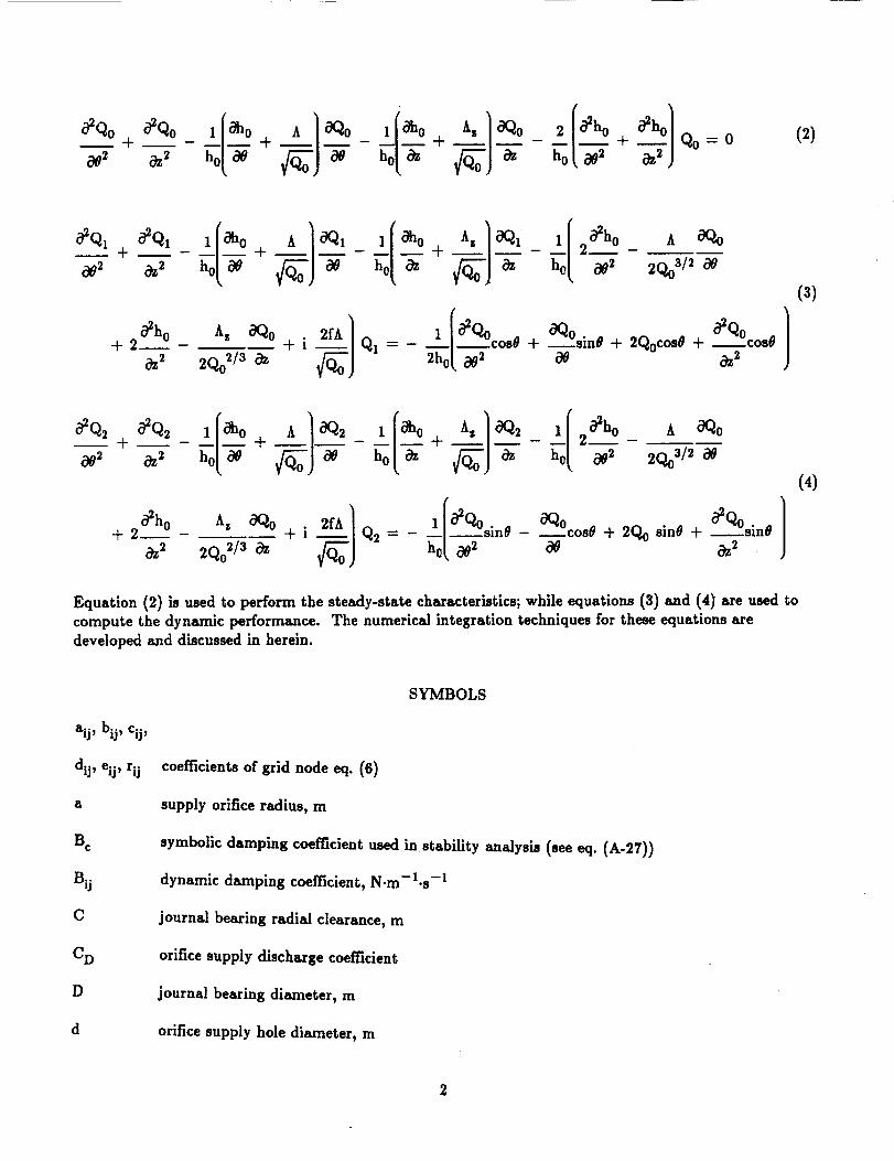
Equation (2)isused to perform the steady-statecharacteristics;while equations(3)and (4)are used to

compute the dynamic performance. The numericalintegrationtechniquesfortheseequationsare

developed and discussedin herein.

aij, bij, cij,

dip eij, rij

:a

B¢

Bij

C

C D

D

d

SYMBOLS

coefficientsof gridnode eq. (6)

supply orificeradius,m

symbolic damping coefficientused instabilityanalysis(seeeq. (A-27))

dynamic damping coefficient,N.m-l.s -1

journalbearingradialclearance,m

orificesupply dischargecoefficient

journalbearingdiameter,m

orificesupply holediameter,m

2

e

emax

F

F

Fr,F t

Fro,Fro

Fx,Fy

f

fo

G m

h

ti"

ho

hm

i

ii

K

K

Kij

Kc, Kco

L .

l

M

M,N

eccentricity (see fig. 1), m

maximumiterationstep error (seeeq. (12))

load capacity (the resulting force of the pressure distribution), N

F / (PaLD) dimensionless load capacity (eq. (18))

component of F along and perpendicular to the centerline_ respectively (see fig. 1)

steady-state component of F

dynamic component of F along x and y directions (see fig. 1)

whirl frequency ratio, u/f_

unstable whirl frequency ratio, Uo/fl

dimensionless supply flow part that is function of Pm/Ps (see eq. (B-11))

dimensionless film thickness, _'/C

film thickness, m

steady-state component of h

film thickness at the supply orifice (see fig. 13)

-11/2 the imaginary unit

the unit vector along xi direction (see fig. 14)

stiffness, N.m -1

dimensionless stiffness (see eq. (21))

dynamic stiffness coefficient

symbolic stiffness coefficient used in stability analysis (see eqs. (A-27) and (A-29))

bearing length, m

length vector part of the C m boundary of integral (B-7) (see also fig. 14)

rotor mass allocated to one bearing; for a symmetric rotor M is half of the rotor mass, kg

corresponding rotor mass, allocated to one bearing, required to make the bearing unstable, kg

number of grid points in i and j directions

n

n O

P

P

Pa

Pla' P2a

Pm

PO

Ps

Pl' P2

Q

Q0, QI, Qu

qm

R

P

r,t

ST

T

t

V,

W

x,y

Xl,3

Zij

g

unit vector outward, perpendicular to the Cm boundary (see nlj in fig. 14)

total number of supply orifices

pressure, Pa

dimensionless pressure

ambient pressure, Pa

boundary pressure at bearing edges

pressure downstream of the supply system

steady-state component of the pressure p (see eq. (A-6))

supply pressure, Pa

perturbation components of pressure p (see eq. (A-6))

dimensionless pressure variable, (ph) z

steady-state and perturbation components of Q (see eq. (A-7))

dimensionless flow through the pocketed orifice supply restrictor system

journal bearing radius, m

gas constant (see eq. (B-9)), J.kg-l.K -1

coordinates (fig. 1)

threshold speed, f/(M c C/W) 1/2

absolutetemperature (seeeq. (B-9)),K

time,s

axialvelocity(shaftspeed along z direction),m.s -I

bearingload,N

whirl amplitude of the journalcenterin bearing (seeeqs.(.4_-20)and (A-25))

fluid film coordinates (see eq. (A-l) and fig. 14)

impedance for translatory motion

axial coordinate parallel to rotor axis

-/

Az

AO

%

%¢1

0

A

Az

As

A

#

v

v 0

T

n

nl

f_2

Subscripts:

r

adiabatic exponent

increment in z direction

increment in 0 direction

pocketed orifice compensation factor, a2/dC

eccentricity ratio, e//R

eccentricity ratio under static load

dimensionless tangential whirl amplitude

dimensionless radial whirl amplitude

angular coordinate from centerline (see fig. 1)

bearing number (see eq. (A-2) and (B-5))

equivalent bearing number in z direction (see eq. (A-2))

restrictor coefficient (see eq. (B-9))

relaxation coefficient (see eq. (10))

dynamic viscosity, N-s.m -2

whirl frequency, rad.s -1

unstable whirl frequency

dimensionless time (see eq. (A- 1))

attitude angle, deg

attitude angle under static load, deg

rotation frequency, rad-s -1

shaft rotation frequency, rad.s -1

bearing housing rotation frequency, rad.s -1

grid index

centerline direction (see fig. 1)

t perpendicular to center-line direction (see fig. 1)

x x-direction (direction of the static load on bearing, see fig. 1)

y y-direction perpendicular to x (see fig. 1)

Superscripts:

n

n+l

(n + 1)/2

old iteration step

new iteration step

half step iteration between n and n + 1

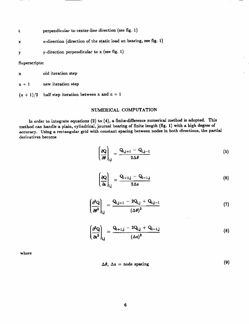
NUMERICAL COMPUTATION

In order to integrate equations (2) to (4), a finite-difference numerical method is adopted. This

method can handle a plain, cylindrical, journal bearing of finite length (fig. 1) with a high degree of

accuracy. Using a rectangular grid with constant spacing between nodes in both directions, the partialderivatives become

"_ ij Qld+12A

_Q) _- qij+l - 2Qid + Qi,j-1

o2ql qi+l,j - 2qi,j -k qi-l,j-:z :j

where

AO, Az = node spacing

(5)

(e)

(7)

(8)

(9)

6

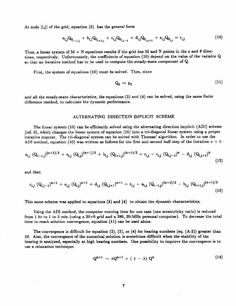
At node (i_) of the grid, equation (2) has the general form

aidQ01_l, j + bidQ0i+t, j + cidQ0ij_l + didQ0ij+l + eijQ0ij = ri. i (10)

Thus, a linear system of M × N equations results if the grid has M and N points in the z and 0 direc-

tions, respectively. Unfortunately, the coefficients of equation (10) depend on the value of the variable Q

so that an iterative method has to be used to compute the steady-state component of Q.

First, the system of equations (10) must be solved. Then, since

Q0 _ p0 (11)

and all the steady-state characteristics, the equations (3) and (4) can be solved, using the same finite

difference method, to calculate the dynamic performance.

ALTERNATING DIRECTION IMPLICIT SCHEME

The linear system (10) can be efficiently solved using the alternating direction implicit (ADI) scheme

(ref. 6), which changes the linear system of equation (10) into a tri-diagonal linear system using a properiterative manner. The tri-diagonal system can be solved with Thomas' algorithm. In order to use the

ADI method, equation (10) was written as follows for the first and second half step of the iteration n + 1:

__ __ n Q naij (Qi_lj) (n+l)/2 W ei_i (Qij) (n+1)/2 + bij (Qi+lj) (n+l)/2 rij cij (Qij-1) - dij (ij+l)

(12)

and then

(Q _n+l n÷l (f-_ _n+l _cij _ ij-lJ -t- el. i (Qij) _ di.i _'_i5+1/ = ri,j aij (Qi-lj) (n+1)/2 - bij (Qi+lS) (n+1)/2

(13)

This same scheme was applied to equations (3) and (4) to obtain the dynamic characteristics.

Using the ADI method, the computer running time for one case Cone eccentricity ratio) is reduced

from 1 hr to 1 to 5 min (using a 20×9 grid and a 386, 20-MHz personal computer). To decrease the total

time to reach solution convergence, equation ill) can be used alone.

The convergence is difficult for equation (2), (3), or (4) for bearing numbers (eq. (A-2)) greater than

10. Also, the convergence of the numerical solution is sometimes difficult when the stability of the

bearing is analyzed, especially at high bearing numbers. One possibility to improve the convergence is to

use a relaxation technique:

qn-t-1 __+ _Qn+l _{_ ( I -- )_) Qn(14)

where

A =0--+ 1

A second possibility is to convert the dimensions of the grid from a large one (e.g., fromNxM = 40x33 or 30x25 or 20x17), used to compute the steady-state component Q0 of the variable

(eq. (A-7)) and the derivatives of Q0 and h0, to a small one (e.g., 10x9) and then to compute the

dynamic components Q1 and Q2 of the variable Q.

Q

LIEBMANN'S ITERATIVE SOLUTION

The discretization of the Reynolds equation results in a large linear system of equations that needs

to be solved. For example, a 20 by 9 grid involves 180 linear algebraic equations like equation (10).There are a maximum of five unknown terms per line in equation (10). For a large-sized grid, many of

the terms will be zero. For such a sparse system, the elimination methods waste significant computer

memory to store zeros. To avoid these difficulties, the LIS method (ref. 7) can be used as an alternativeto ADI. In this technique equation (10) is expressed as

Rij - Aij Qi-lj - Bij Qi+lj - Cij Qij-1 - Dij Qij+l

Qij : EiJ

(15)

and solved iteratively for j = 1 to N and i = 1 to M. Because equation (10) is diagonally dominant

for most of the bearing running conditions, this procedure will eventually converge to a stable solution.Note that the coefficients C, D, and E depend on the value of the variable Q from the previous

iteration. As with the ADI method, a relaxation technique can be used to improve the convergence of

this method. The relaxation coefficient, A, can be variable and under control of the maximum error for

each iterationstepcalculatedas

¢hnax-Max(16)

for

i= 1--,M, j = 1-* N (17)

One of the most difficult cases regarding the convergence is the hybrid, compressible-fluid, film

bearing. This case balances the flow through the supply restriction system with the flow through thefluid film to calculate the downstream pressure in the supply port. This requires an additional iteration

loop. Also, the equation of the flow through a restriction system, like a pocketed orifice, is a combinationof four relations that is a function of the type of flow (choked or unchoked) and the direction of the flow

(in or out). The analysis of a hybrid, compressible fluid bearing is outlined in appendix B.

RESULTS AND DISCUSSION

ADI Method

Both steady-stateand dynamic performance resultsover a range of bearingnumber A (A-3) from

0.903 to 9.03 and an eccentricityratiobetween 0.1 and 0.6are very closeto known computed data from

(refs.8 and 9). Figures2 and 3 show the basicsteady-statecharacteristics:loadcapacityand attitude

angle (fig.I and eq. (A-19))versusbearingnumber. The dimensionlessform of the load capacityis

F __

P

PaLD

(18)

The numerically computed steady-state data using the ADI method agree well with Raimondi data

(ref. 8) for both grid dimensions used (20x9 and 10×5). The same conclusion arises in figures 4 and 5where the whirl frequency ratio and threshold speed criteria are shown. The whirl frequency ratio is

v 0f0 = -- (19)

fl

and the threshold speed is

i McC

ST = fl McC = fl (20)

w wpaLD

The notation used in equations (19) and (20) are described in appendix A. In figures 4 and 5 the ADI

computed data are compared with Chang and Pan's computed data (ref. 9). An exception to this general

conclusion may be for the threshold speed at low bearing numbers and especially at small eccentricity

ratios (left bottom corner of fig. 5) where the ADI computed data show more sensitive behavior to the

"half frequency instability" than the data from Chang and Pan. No experimental data were found for

this particular range of input data.

LIS Method

The LIS method is first used to compute the steady-state performance of an aerodynamic journal

bearing. To assess the accuracy of the LIS method, both LIS and Raimondi data are shown in figure 6

for load capacity and in figure 7 for attitude angle. Very good agreement was obtained for a range of the

bearing numbers between 0.1 and 17. The grid has 30x9, 40x9, and 60x9 nodes, and the computing

time for one case (one point in either fig. 6 or 7) is regularly less than 1 min.

The LIS hybrid gas bearing code was first used to compute the steady-state characteristics of a

double-plane supply aerostatic journal bearing with a length to diameter ratio L/D of 2. The output

data for the dimensionless stiffness as was defined in (ref. 10) as

K __

1_-6 2 CK

1 + 2 62 (p,- Pa) LD3

(21)

versus restrictor coefficient (eq. (B-9)) was plotted in figure 8. The notation used in equation (21) is

shown in appendix B. Based on an average stiffness calculation, the eccentricity of the shaft was 0.05,

0.1, and 0.5 of the radial clearance (curves LIS 0.05, 0.1, and 0.5 respectively). For comparison, the

corresponding curve from Wilcock (ref. 10) and Pink's experimental data (ref. 11) are also plotted in

figure 8. Pink's data (ref. 11) were obtained using the stiffness near zero eccentricity and the load at 0.5

eccentricity. The LIS computed data agree well with Pink's experimental data.

The computed total load and stiffness for a hybrid journal gas bearing is shown in figures 9 and 10.

Both externally pressurized and dynamic effects contribute to pressure rises in the fluid film. The

dynamic effects contribute a significant amount to the total load, especially at high eccentricity ratios

and high speeds. Figure 10 and especially figure 11 indicate that, for small eccentricity ratios (near zero),

the dynamic effects can diminish the bearing performance in turning the shaft at low speeds. The radialflow due to the rotation of the shaft appears to change the externally supplied flow. This change results

in the load and stiffness of the hybrid bearing (turning speeds of 5000 and 15000 rpm) being lower than

the aerostatic bearing curve (0 rpm) for eccentricity ratios 0 to 0.2. This phenomenon is controlled by

the turning speed and by the radial clearance ratio. Figure 11 shows how radial clearance affects the

bearing stiffness for turning speeds of 0 and 5000 rpm.

CONCLUSIONS

Two methods (alternating direction implicit (ADI) and Ziebmann's iterative solution (LIS)) were

adopted and modified to integrate the compressible pressure-differential equation. The ADI method was

used to compute the steady-state and the dynamic performance of an aerodynamic journal bearing. Both

steady-state and dynamic results are in good agreement with known design criteria. The LIS methodwas used to calculate the pressure distribution of a hybrid journal gas bearing. Because a hybrid bearing

needs an additional iteration loop to balance the flow through the supply system with the flow through

the lubrication film, convergence takes longer. Both numerical methods (ADI and LIS) are more

efficient, in terms of running time of the codes, than other known methods. However, the ADI method

sometime shows poor convergence, especially for dynamic computation at very low or very high bearingnumbers. The LIS method can handle the aerodynamic, the aerostatic, and the hybrid bearings and can

generate useful data, especially for hybrid gas bearings. Furthermore, the LIS method can provide data

with minimal computer time. Both methods (ADI and LIS) provide data with running computing timesbetween 10 to 50 times faster than other methods that involve inverting a matrix. The running time for

the ADI or LIS method is proportional to the grid dimension.

ACKNOWLEDGMENTS

This paper arises from the work done at the NASA Lewis Research Center, Cleveland, Ohio, in a

NRC Associateship Program. I would like to thank Jim Walker, Gene Addy, and David Brewe from

NASA Lewis who kindly reviewed this paper and D. Vijayaraghavan for his suggestions concerning theADI method.

10

APPENDIX A. -- STEADY-STATE AND DYNAMIC ANALYSES OF A PLAIN, CYLINDRICAL,

FINITE LENGTH, SELF-ACTING GAS JOURNAL BEARING.

The Reynolds equation in dimensionless form for a compressible-fluid-film journal bearing subject to

isothermal conditions is (refs. 4 and 5)

(1)

where

p= __,P 0= __, z= __ r=ivt, =

Pa R R

(A-l)

A = p: p. R[cJ(A-2)

f = _v (12 = n I ÷ n2) (A-3)fl

and where _1 is the shaft rotating speed, l] 2 is the bearing rotating speed, y is the whirl frequency (in

radians per second), Yz is the shaft axial speed, and p is the dynamic viscosity.

Both circumferential and axial movement are taken into account in equation (A-l), and a complex

form for time-dependent terms is used for the dynamic analyses.

In order to integrate equation (1), a natural linearization procedure is applied (ref. 1) by writingReynolds equation in terms of a new variable Q -- (ph) 2. For the dynamic analyses, a small perturba-

tion technique was used. Here, the journal center was assigned a static eccentricity ratio •0 and a

corresponding attitude angle ¢0" This position was perturbed by a small amplitude harmonic motion:

• : e0 _ •1er, _o : @0 _ _PleT (A-4)

The corresponding perturbed forms of the dimensionless film thickness and pressure can be written as

h : h0 + •1 er COS 0 + •0_O1er sin 0 (A-5)

P : Po "-t-•1e_"Pl -I- •01Olev P2 (A-6)

11

Introducinga new variable

q = (Ph) 2 = Qo + 2 ¢1ez Q1 + 2 ¢0tOler Q2 (A-7)

and substituting equations (A-5), (A-6), and (A-7) into equation (1) yield

+_- ho[00 "_'- h0[& _-_-'J _ - _o 00''_-+ o_2J

Q0 =0 (2)

+-_- ho(o_ +_J-_-- _oo _'+ -_-- _ -_-

A OQo!

2Q03/2 0e

_h o A, aQ o 2fA ]+2__ - +i

Oz2 2Qo 2/30z _oJ

OQo a2QocosO+ __sin0 + 2QocosO +/_ az 2

(3)

lf*_. __ a2QOsinO

+ 2/_h0__.- 2Q_13_A'_ +i .j2fA]Q' =- _[l_ -slnO °Q°c°s°-I 2Q°sinO+_ az2

(4)

The equation (2) is the conventional steady-state equation. It is nonlinear and was solved in finite-difference form by an iterative method. The last two equations depend on the steady-state solution.

They are linear equations with complex dependent variables and were solved numerically.

Taking into account equations (A-5), (A-6), and (A-7) the following relations can be established:

Qo = P02h02

Q1 ! Po2ho cos 0 + P0h02Pl (A-S)

Q2 l p02h0 sin 0 + poh02p2

12

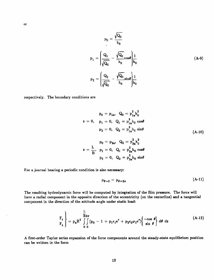
or

Pl =

P2 =

P0--h0

(A-9)

respectively. The boundary conditions are

z:O_

L

z:_,

2 2PO ----Pla, Qo -- Plaho

2Pl : O, Q1 = Plaho cosO

2P2 = 0, Q2 = Plaho sinO

2 2Po = P2a, Qo = P2aho

2Pl -" 0, Q1 = P2aho cosO

2P2 = 0, Q2 = P2aho sin0

(A-10)

For a journal bearing a periodic condition is also necessary:

PO=O = Po=2r (A-11)

The resulting hydrodynamic force will be computed by integration of the film pressure. The force will

have a radial component in the opposite direction of the eccentricity (on the centerline) and a tangential

component in the direction of the attitude angle under static load:

F r

Ft

L

-cos: p_R2 f f (Po - 1 + Pl'le' + P2'o_,e_ sin O j00

d0 dz(A-12)

A first-order Taylor series expansion of the force components around the steady-state equilibrium positioncan be written in the form

13

where

Fr = Fro + Zrr el e_ + Zrt Co _1 er

Ft = Ft0 -{- Ztr _1 e_ ÷ Ztt e0 _1 e_

Zij : Kij +i v Bij

i = r,t; j = r,t

(A-13)

(A-14)

are the bearingimpedances. From equations(A-12)and (A-13)the steady-stateforcecomponents and

the impedance coefficientsare

L

{co., Fro R2Ft 0 =Pa ff (P0-1) sin @j

00

d# dz(A-15)

Zl_r

Ftr

L

R2f

-cos=Pa R' ff Pl sinOJoo

dO dz(A-16)

Zrt

Ztt

L

R2¢

{-¢o.°1,=P. R2 ff P, sin#j d#dzOO

(A-17)

The steady-stateforceis

F -- _Fro 2 + Fro2; W = -F (A-18)

where F is the load capacity of the bearing and W is the bearing load. The angle between the force F

and the centerline axis is defined by the equation

Fro= tan-1 (A-19)Ft0

Under dynamic conditions, the journal (shaft) center whirls in an orbit around its static equilibrium

position. The corresponding dynamic bearing reaction is actually a nonlinear function of the amplitude

and depends implicitly on time. In a thorough analysis it is necessary to consider the rotor and the

bearing simultaneously as was done, for example, in the reference 12. In most practical situations, the

amplitude of the shaft motion is, of necessity, rather small. In these cases a linearization of the bearing

14

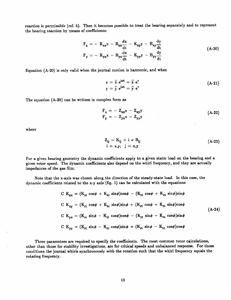
reactionis permissible (ref. 5). Then it becomes possible to treat the bearing separately and to represent

the bearing reaction by means of coefficients:

B dx Bx-dyFx = - Kxxx - xx_-_ - KxyY - Ydt

=- - B dx - Kyyy- Byyd-_yFy KyxX YXd=_ d_

(A-20)

Equation (A-20) is only valid when the journal motion is harmonic, and when

x = e = e

y = y e ivt = y eT

(A-21)

The equation (A-20) can be written in complex form as

Fx-- _ Zxxx- ZxyY

Fy = - Zyxx - Zyyy

(A-22)

where

Zij = Kij + i u Bij (A-23)

i = x,y; j =x,y

For a given bearing geometry the dynamic coefficients apply to a given static load on the bearing and a

given rotor speed. The dynamic coefficients also depend on the whirl frequency, and they are actually

impedances of the gas film.

Note that the x-axis was chosen along the direction of the steady-state load. In this case, the

dynamic coefficients related to the x-y axis (fig. 1) can be calculated with the equations

C Kxx = (Krr cosS+ Ktr sinS)tosS - (Krt cosS+ Ktt sinS)sinS

C Kxy

C Ky x

= (Krr cosS + Ktr sinS)sinS + (Krt cosS + Ktt sinS)tosS

= (Krr sins - Ktr cosS)cosS - (Krt sins - Ktt cosS)sinS

(A-24)

C Kyy = (Krr sins - Ktr tosS)sinS + (Krt sins - Kit cosS)cosS

Three parameters are required to specify the coefficients. The most common rotor calculations,

other than those for stability investigations, are for critical speeds and unbalanced response. For those

conditions the journal whirls synchronously with the rotation such that the whirl frequency equals the

rotating frequency.

15

C B_ = (Brr cos# + Btr sin#)cos# - (Brt cos# + Btt sin#)sin#

C Bxy = (Brr cos# + Btr sin#)sin# + (Brt cos# + Btt sin#)cos#

1/v

C By x _- (Brr sin# - Btr cos#)cos# - (Brt sin# - Btt cos#)sin#1/v

(A-50)

C Byy : (Brr sin# - Btr cos#)sin# + (Brt sin# -Btt cos# )cos#

1/v

In a stability calculation, it is necessary to evaluate the bearing coefficients over a frequency range,

usually around one half of the rotating frequency. On the basis of these values, a stability analysis can be

performed. If M is the rotor mass supported by the bearing (M = 1/2 of the rotor mass when the rotor is

symmetric and rigid) and the bearing is represented by its four Z impedance coefficients, the motion

equation can be written as

1z M2zxy]ixlZyx (Zyy-Mv 2) Y

---- 0 (A-26)

The threshold of instability occurs when the determinant of the matrix is zero. Noting that

Z = K e + it'B c, K e =My z (A-27)

we can solve the determinant equation to get

_ _ d 41 (Zxx _ Zyy)Z ___ Zxy Zy x (A-28)Z = 1 (Zxx ___Zyy) --2

(For stability calculations only the solution with a negative sign in front of the square root proves to be

of interest (ref. 5).) At the threshold of instability, Z must be real. The imaginary part of Z can be

evaluated over a range of frequencies to find that frequency value v 0 at which the imaginary part of Z is

zero. The corresponding mass is the mass required to make the bearing unstable under the selected

working conditions and is

Kc° (A-29)

//02

16

APPENDIX B--HYBRID GAS JOURNAL BEARING ANALYSIS

The geometry and notation for a double-plane, externally pressurized journal bearing is shown in

figure 12. The Reynolds equation for steady-state condition of a gas journal bearing becomes

(]3-1)

Supposing an isothermal evolution of the gas such that

P ----constant

P

(]3-2)

and using the new natural linearization variable

q = (ph) 2 (B-3)

equation (B-l) may be written as

h002 2h(Q(n)_/2 - Q(n+I)= A 1

(B-.4)

where the bearing number is

Equation (B-4) is written for two successive iterations. To improve the convergence due to the nonlinear

terms of the compressible Reynolds equation, a Newton-Raphson method

f(nw1)[q,__} __ f(n){Q,___} ..__ {._}(n)_Q_l_ f o_ /(n)A/()Q] (B-6)

is used to write equation (B-4).

17

Equation (B-4) is valid for all points covering a bearing grid except the edges and the fluid supply

points. For a pocketed orifice restrictor supply system (fig. 13), the flow through the supply restrictorand through the film has to be balanced to calculate the pressure downstream of the supply restrictor:

( Aph _'1 - Rh3p Vp ) n d_ = qm (]3-7)

Cm

The left side of the equation (]3-7) represents the flow through the film. For computational convenience

the supply hole geometry is slightly modified as shown in figure 14. The right side of the equation (13-7)

is the flow through the supply orifice restrictor:

where the restrictor coefficient is

2rA. p2 / 1 + _i2qm -- hmGm (B-8)

n I h2 + 62m

- 6J' °a2 I (B-g)A.psC 3 _ 1 + 62

and

a2 (B-10)

dC

Gm = C D

I ( _ "/+1

(7+1)

["_) tP,) J

tPm) tPm)

if Pm< 2

p---:-- ['_-'_)

_,7+11 p.

if P_.._m> 1

Ps

(B-n)

18

CD---- 1

C D = 1.155 - 0.555

p. 1,7 + 1)

f /'ifPm > 2 _-I

(B-12)

The discharge coefficient C D (B-12) was established taking into account data from references 4 and 10.

Note that Pm is the pressure downstream of the supply system and Ps is the supply pressure.

Having a first-guess pressure distribution, the pressure Pm can be calculated with equation (]3-7) and

used like a boundary condition for equation (B-4) in the next iteration.

19

REFERENCES

1. Castelli, V.; and Pirvics, J.: Review of Numerical Methods in Gas Bearing Film Analysis. J. Lub.

Technol., vol. 90, Oct. 1968, pp. 777-792.

2. ]_oy, M.L.: A Noniterative Numerical Solution of Poisson's and Laplace's Equations with

Application to a Slow Viscous Flow. J. Basic Eng., vol. 88, no. 4, Dec. 1966, pp. 725-733.

3. Coleman, R.: The Numerical Solution of Linear Elliptic Equations. J. Lub. Technol., vol. 90,

Oct. 1968, pp. 773-776.

4. Gross, W.A.: Fluid Film Lubrication. Wiley, 1980.

5. Lund, J. W.: Calculation of Stiffness and Damping Properties of Gas Bearings. J. Lub. Technol.,

vol. 90, Oct. 1968, pp. 793-803.

6. Vijayaraghavan, D.; and Keith, T.G., Jr.: An Efficient, Robust and Time Accurate Numerical

Scheme Applied to a Cavitation Algorithm. J. Tribol., vol. 112, Jan. 1990, pp. 44-51.

7. Chapra, S.C.; and Canale, R.P.: Numerical Methods for Engineers. Second ed., McGraw-Hill, 1988,

Ch. 23, pp. 715-732.8. Raimondi, A.A.: A Numerical Solution for the Gas-Lubricated Full Journal Bearing of Finite

Length. Trans. ASLE, vol. 4, 1961, pp. 131-155.9. Chang, H.S.; and Pan, C.H.T.: Stability Analysis of Gas-Lubricated, Self-Acting, Plain, Cylindrical,

Journal Bearings of Finite Length Using Galerkin's Method. J. Basic Eng., vol. 87, Ser. D, no. 1,

Mar. 1965, pp. 185-192.10. Pink, E.G.: An Experimental Investigation of Externally Pressurized Gas Journal Bearings and

Comparison with Design Method Predictions. Prec. 7th Intern. Gas Bearing Symp., Churchill

College, Cambridge, England, July 13-15, 1976, pp. G3-41 to G3-59.11. Wilcock, D.F., ed.: Gas Bearing Design Manual. Mechanical Technology, Inc., Latham, New York,

1972.

12. Castelli, V.; and McCabe, J.T.: Transient Dynamics of a Tilting Pad Gas Bearing System. J. Lub.

Technol., Ser. F, vol. 89, no. 4, Oct. 1967, pp. 499-509.

2O

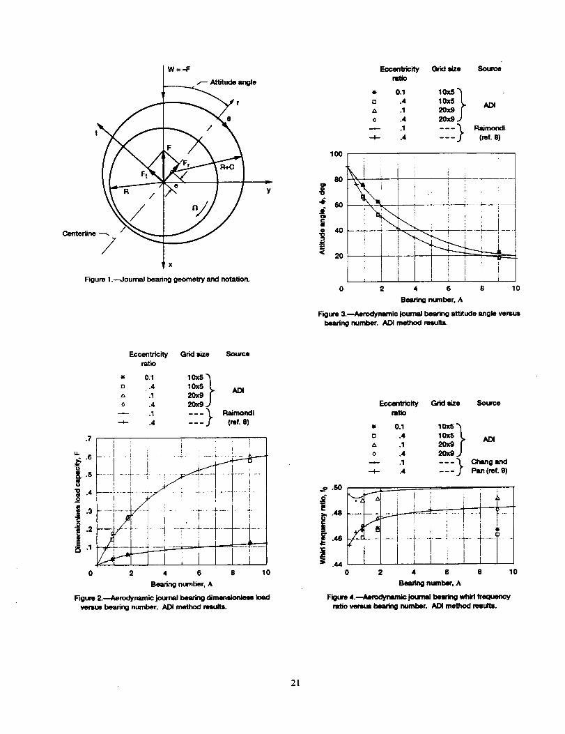
W=-F

_-- Attitude angle

r

e

Center_rm --_

/x

ngum 1.--4oumal bearing geometry _ notation.

Eccenfficity Grid ize Sourcemtlo

0.1 10x5 "_

c3 .4 10x5 ._ ADIA .1 20x9o .4 20x9

.1 -- - "_ RaJmondi

-_- .4 j" (ref. e)

i !

80 I :! i ! I

"_ 60 _, I i •

-_ ! i , i

• 4o - -- _ _"_i--;--i--

<= 20 i t I _ 7-'--__L i, I t

0 2 4 6 8 10

Bearing number, A

Figure 3._Aerodynamic journal bearing attitude angle versusbearing number. ADI method results.

.7

u.- o6

i.3

"_ .2

Ei5 .1

Eccentricity Grid sizeratio

w, 0.1 10X5 •[3 .4 10X5

.1 20x90 .4 20x9 •

-- _ ---}--I-- .4

Source

ADI

Raimondi(ref. e)

I i , I : I , I

L.: -i- i .... _..... _ ..!-- ,L._.

t'!m

0 2 4 6 10

Bearing number, A

Figure 2..--Aerodynamic journal bearing dimemdonleN loadvenous bearing number. ADI method re_Jlts.

Eccentricity Grid size Sourcemtk_

0.1 10x5 "_

o .4 10xS _. ADI.1

0 .4

--;-- .4 Pan (inf. 9)

• I i __4.!....

..I 1 /0 2 4 6 8 10

Bering number, A

Figure 4.--Aerodynamic jourmd beari_ whirl frequencyratio versus bearing number. ADI method results.

21

Eommtrk:_ Gdd aize Soumemtb

r-, .4 10x6 ADI,'_ .1o .4

.4 Pan (mr. 9)

2.5

2.o -- __

J 1.0 f

0 2

Bewtng nmnl_, A

F_ureS.--Aerodyrwnlcjourr_txmr_ thre_Id speedvemm bearing number. ADI method results.

E(:_ent_ity Grid size Sourceraio

0.130x960x_ 1

o .4 _40x_x .1 USo .4z .1

.4

-- .1 ---} P.. i-+- .4 (_. 8)

t 1 ' loo ' " ! _ i iJ

!_I "_\t i i ! i i i ;

I ....... I "

14 6 8 10 0 2 4 6 8 10 12 14 16 18 20

Bmdng number, A

Figure 7.---A_0dymmlc journal heroin0 attitude angleversus beming manber. US data.

.7

i "+.8

.4

i +.2.1

Eccentricity Grid lize Sourcemtio

00 .4 _x .1 US0 .4

.1E

_, .4

-- .1 - - - _ Raimondi

-_- .4 --- j (_. e)

0 2 4 6 8 10 12 14 16 18 20

Bering number, A

FeureS.--JWodymm_jo,m_ bem_0d_nen,_mload remus buring number. US da_

Data Eccentricity Source

.... Design data_.oc_ ref. 11)

0.05.10 US

-e- .50

x 0 "_ Expedrnent datao .80 J (Pink, ret. 10)

_ ;_ _-.J-+ + + _ J

.01.001 .01 .1 1 10

Figure 8._,,omptd!_ of US oompubKI _tlflne_ with ckmignd_t_ snd expedmental d_ta. Aerosta_: joumsl bearing;

prmmum ratio P_/Pm 8; length to diameter m_o, L/D, 2;do.hie_up_y p_ne;zero_peed.

22

3OOO

Tumng.be_

rpm

050OO

15000--e- 50000

100000

Z 2OOO

o 1500"d

...... L- + i +_ _._+-

I ' ' F ( ! /...... [+ i .... _ _+-__ _ .....

0 .I .2 .3 .4 .5 .6 .7 .8

Eccentricity ratio

Figure 9.--Total load versus eccentricity ratio as function offuming speed. Hybrid air bearing; length, L, 100 mm;diameter, D, 50 mm; radial clearance, C, 0.02 mm; doublesupply plane; supply pressure, Pt, 0.5 MPIL

Turr.ngIpeed,

rpm

-- 050O0

15000--e- 50000--- 100000

160I J t

............... _ ..... i+ __ +_

i 80 ........ r--- ,

0 .1 .2 .3 .4 .5 .6 .7

Ecc_triclty ratio

Figure 10.--Stiffness remus eocentdc_ ratio m function ofturning speeds. Hybrid air bearing; length, L, 100 mm;diameter, D, 50 mm; radial clearance, C, 0.02 mm; double

supply plane; supply pressure, pm 0.5 MPL

.8

Radial Turningm, =pee_

mm q)m

0.020 0--e- .020 5000

.015 0--e- .015 5000

.010 0

.010 5000

160

80 ---

4o _ b I

t0 .1 .2 .3 .4 .5

Ec_mb'icity ratio

Figure 11.---Stiffness versus eccentricity ratio as functionof radial cleeranoe at two turning speeds. Hybrid journalbearing; length, L, 100 mm; diameter, D, 50 ram; doublesupply plane; supply pressure, p,,.0.05 MPL

23

Figure 12.--ExtemmJly prusudzed gas journmJbemdng geometryand notat_

Ps /-- Orifioe

J k'_\\\\\\\\'_

i

Joum_

hm

Figure 13.--Supp#y orir_m zorn. geomeW ,,,rid not_Ik)n.

x3 ,zR

Supplyo_ke .-_ i

D ..X" ,. C

.... -A_al=upptypor.ket-J tNAB ",

I

_BC

B V

"-- Assumed supplypooket

"_ xl.eR

F',eur.14.--Sumb odr_epocket,_/m _.umpt_.

24

Form ApprovedREPORT DOCUMENTATION PAGE OMB No. 0704-0188

Public reporting burden for this collect_n of information is estimated to average 1 hour per response, including the time for reviewing instructions, searching existing data sources,

gathering and maintaining the data needed, and completing and reviewing the collection of information. Send comments regarding this burden esUmate or any other aspect of this

collection ol information, including suggestion,s for reducing this burden, to Washington Headquarters Services, Directorate for information Operations and Reports, 1215 Jefferson

Davis Highway, Suite 1204, Arlington. VA 22202--4302, and to the Office of Management and Budget, Paperwork Reduction Proiect (0704-0188), Washington, DC 20503.

I. AGENCY USE ONLY (Leave blank) 2. REPORT DATE 3. REPORT TYPE AND DAI-I:_ COVERED1992 Technical Memorandum

5. FUNDING NUMBERS4. TITLE AND SUBTITLE

Fast Methods to Numerically Integrate the Reynolds Equation for Gas

Fluid Films

6. AUTHOR(S)

Florin Dimofte

7. PERFORMING ORGANIZATION NAME(S) AND ADDRESS(ES)

National Aeronautics and Space Administration

Lewis Research Center

Cleveland, Ohio 44135-3191

9. SPONSORING/MONITORING AGENCY NAMES(S) AND ADDRESS(ES)

National Aeronautics and Space Administration

Washington, D.C. 20546-0001

WU-590-21-11

8. PERFORMING ORGANIZATIONREPORT NUMBER

E-6824

10. SPONSOR ING/MONFi'O_ii'IGAGENCY REPORT NUMBER

NASA TM- 105415

11. SUPPLEMENTARY NOTES

Prepared for presentation at the STLE-ASME Joint Tribology Conference, St. Louis, Missouri, October 13-16, 1991.

Florin Dimofte, National Research Council-NASA Research Associate at Lewis Research Center. Responsible

person, Florin Dimofte, (216) 977-7486.

12_ DISTRIBUTION/AVAILABILITY STATEMENT

Unclassified - Unlimited

Subject Category 37

12b. DI_i_IBUTION CODE

13. ABSTRACT (Maximum 200 words)

The alternating direction implicit (ADI) method is adopted, modified, and applied to the Reynolds equation for thin, gas

fluid films. An efficient code is developed to predict both the steady-state and dynamic performance of an aerodynamic

journal bearing. An alternative approach is shown for hybrid journal gas bearings by using Liebmann's iterative solution

(LIS) for elliptic partial differential equations. The results are compared with known design criteria from experimental

data. The developed methods show good accuracy and very short computer running time in comparison with methods

based on an inverting of a matrix. The computer codes need a small amount of memory and can be run on either per-

sonal computers or on mainframe systems.

14. SUBJECT TERMS

Tribology; Reynolds equation; Gas fluid film; Hybrid gas journal bearing; Aerodynamic

gas journal bearing; Alternating direction implicit method; Liebmann's iterative solution

17. SECURITY CLASSIFICATION

OF REPORT

Unclassified

NSN 7540-01-280-5500

18. SECURITY CLASSIFICATION

OF THIS PAGE

Unclassified

19. SECURITY CLASSIRCATION

OF ABSTRACT

Unclassified

15. NUMBER OF PAGES26

16. PRICE CODE

A03

20. UMITATION OF ABSTRACT

Standard Form 298 (Rev. 2-89)

Prescribed by AN S I Std. Z39-18:)98-102