fast fourier transform (fft) - in.tum.de filea fast computation is possible via the...

Algorithms of Scientific Computing

Fast Fourier Transform (FFT)

Michael BaderTechnical University of Munich

Summer 2018

The Pair DFT/IDFT as Matrix-Vector Product

DFT and IDFT may be computed in the form

Fk =1N

N−1∑n=0

fnω−nkN fn =

N−1∑k=0

FkωnkN

or as matrix-vector products

F =1N

WH f , f = WF ,

with a computational complexity of O(N2).

Note thatDFT(f ) =

1N

IDFT(f ) .

A fast computation is possible via the divide-and-conquer approach.

Michael Bader | Algorithms of Scientific Computing | Fast Fourier Transform (FFT) | Summer 2018 2

Fast Fourier Transform for N = 2p

Basic idea: sum up even and odd indices separately in IDFT

→ first for n = 0,1, . . . , N2 − 1:

xn =N−1∑k=0

XkωnkN =

N2−1∑k=0

X2kω2nkN +

N2−1∑k=0

X2k+1ω(2k+1)nN

We set Yk := X2k and Zk := X2k+1, use ω2nkN = ωnk

N/2, and get a sum of twoIDFT on N

2 coefficients:

xn =N−1∑k=0

XkωnkN =

N2−1∑k=0

YkωnkN/2︸︷︷︸

:= yn

+ωnN

N2−1∑k=0

ZkωnkN/2︸︷︷︸

:= zn

.

Note: this formula is actually valid for all n = 0, . . . ,N − 1; however, the IDFTs of size N2 will only

deliver the yn and zn for n = 0, . . . , N2 − 1 (but: yn and zn are periodic!)


Fast Fourier Transform (FFT)

Consider the formular xn = yn + ωnNzn for indices N

2 , . . . ,N − 1 :

xn+ N2= yn+ N

2+ ω

(n+ N2 )

N zn+ N2

for n = 0, . . . , N2 − 1

Since ω(n+ N

2 )N = −ωn

N and yn and zn have a period of N2 , we obtain the

so-called butterfly scheme:

xn = yn + ωnNzn

xn+ N2

= yn − ωnNzn

zn yn − ωnzn

yn yn + ωnzn

ωn


Fast Fourier Transform – Butterfly Scheme

(x0, x1, . . . , . . . , xN−1) = IDFT(X0,X1, . . . , . . . ,XN−1)

⇓(y0, y1, . . . , y N

2−1) = IDFT(X0,X2, . . . ,XN−2)

(z0, z1, . . . , z N2−1) = IDFT(X1,X3, . . . ,XN−1)

yy0

yy1

zz0

zz1 x3

x2

x1

x0y0

y1

z0

z1X3

X1

X2

X0X0

X1

X2

X3


Fast Fourier Transform – Butterfly Scheme (2)

X0

X1

X2

X3

X4

X5

X6

X7

X0 X0

X2

X4

X6

X1

X3

X5

X7

X2

X4

X6

X1

X5

X7

x 4(4)

x 0(0)

x 7(7)

x 3(3)

x 5(5)

x 1(1)

x 6(6)

x 2(2)

X3

x 0(0−6)

x 2(0−6)

x 4(0−6)

x 6(0−6)

x 1(1−7)

x 3(1−7)

x 5(1−7)

x 7(1−7)

x 3(3,7)

x 7(3,7)

x 5(1,5)

x 1(1,5)

x 6(2,6)

x 2(2,6)

x 4(0,4)

x 0(0,4) x 0

x 2

x 1

x 5

x 6

x 4

x 7

x 3


Recursive Implementation of the FFT

rekFFT(X) −→ x

(1) Generate vectors Y and Z:

for n = 0, . . . , N2 − 1 : Yn := X2n und Zn := X2n+1

(2) compute 2 FFTs of half size:

rekFFT(Y) −→ y and rekFFT(Z) −→ z

(3) combine with “butterfly scheme”:

for k = 0, . . . , N2 − 1 :

{xk = yk + ωk

Nzk

xk+ N2

= yk − ωkNzk


Observations on the Recursive FFT

• Computational effort C(N) (N = 2p) given by recursion equation

C(N) =

{O(1) for N = 1O(N) + 2C

(N2

)for N > 1

⇒ C(N) = O(N logN)

• Algorithm splits up in 2 phases:• resorting of input data• combination following the “butterfly scheme”

⇒ Anticipation of the resorting enables a simple, iterative algorithm withoutadditional memory requirements.


Sorting Phase of the FFT – Bit Reversal

Observation:

• even indices are sorted into the upper half,odd indices into the lower half.

• distinction even/odd based on least significant bit• distinction upper/lower based on most significant bit⇒ An index in the sorted field has the reversed (i.e. mirrored) binary

representation compared to the original index.


Sorting of a Vector (N = 2p Entries, Bit Reversal)/∗∗ FFT sorting phase: reorder data in array X ∗/for( int n=0; n<N; n++) {

// Compute p−bit bit reversal of n in jint j=0; int m=n;for( int i=0; i<p; i++) {

j = 2∗j + m%2; m = m/2;}// if j>n exchange X[j] and X[n]:if ( j>n) { complex<double> h;

h = X[j ]; X[ j ] = X[n]; X[n] = h;}

}Bit reversal needs O(p) = O(logN) operations

⇒ Sorting results also in a complexity of O(N logN)

⇒ Sorting may consume up to 10–30 % of the CPU time!


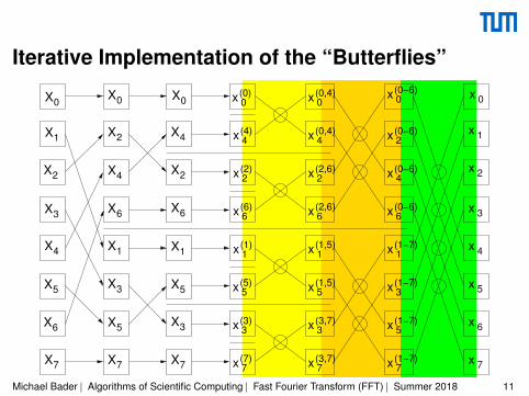
Iterative Implementation of the “Butterflies”

X0

X1

X2

X3

X4

X5

X6

X7

X0 X0

X2

X4

X6

X1

X3

X5

X7

X2

X4

X6

X1

X5

X7

x 4(4)

x 0(0)

x 7(7)

x 3(3)

x 5(5)

x 1(1)

x 6(6)

x 2(2)

X3

x 0(0−6)

x 2(0−6)

x 4(0−6)

x 6(0−6)

x 1(1−7)

x 3(1−7)

x 5(1−7)

x 7(1−7)

x 3(3,7)

x 7(3,7)

x 5(1,5)

x 1(1,5)

x 6(2,6)

x 2(2,6)

x 4(0,4)

x 0(0,4) x 0

x 2

x 1

x 5

x 6

x 4

x 7

x 3


Iterative Implementation of the “Butterflies”

{Loop over the size of the IDFT}for(int L=2; L<=N; L*=2)

{Loop over the IDFT of one level}for(int k=0; k<N; k+=L)

{perform all butterflies of one level}for(int j=0; j<L/2; j++) {{complex computation:}z ← ω

jL * X[k+j+L/2]

X[k+j+L/2] ← X[k+j] - z

X[k+j] ← X[k+j] + z

}

• k-loop und j-loop are “permutable”!• How and when are the ωj

L computed?


Iterative Implementation – Variant 1

/∗∗ FFT butterfly phase: variant 1 ∗/for( int L=2; L<=N; L∗=2)

for( int k=0; k<N; k+=L)for( int j=0; j<L/2; j++) {

complex<double> z = omega(L,j) ∗ X[k+j+L/2];X[k+j+L/2] = X[k+j] − z;X[k+j] = X[k+j] + z;

}Advantage: consecutive (“stride-1”) access to data in array X

⇒ suitable for vectorisation⇒ good cache performance due to prefetching (stream access) and usage

of cache lines

Disadvantage: multiple computations of ωjL


Iterative Implementation – Variant 1 Vectorised

/∗∗ FFT butterfly phase: variant 1 vectorised∗/for( int L=2; L<=N; L∗=2)

for( int k=0; k<N; k+=L)for( int j=0; j<L/2; j+= SIMD LENGTH) {

kjStart = k+j ;kjEnd = k+j + (SIMD LENGTH−1);complex<double> z[0: SIMD LENGTH−1];z[0: SIMD LENGTH−1] = omega(L,j) ∗ X[kjStart+L/2 : kjEnd+L/2];X[kjStart+L/2 : kjEnd+L/2] = X[kjStart :kjEnd] − z;X[kjStart :kjEnd] = X[kjStart :kjEnd] + z;

}

Comments on the code:

• we assume that our CPU offers SIMD instructions that can add/multiply short vectors ofSIMD LENGTH complex numbers

• with the notation X[kjStart :kjEnd] we mean a subvector of SIMD LENGTH consecutivecomplex numbers starting from element X[kjStart ]

• Note: the term omega(L,j) has to changed into such a short vector, as well


Iterative Implementation – Variant 2

/∗∗ FFT butterfly phase: variant 2 ∗/for( int L=2; L<=N; L∗=2)

for( int j=0; j<L/2; j++) {complex<double> w = omega(L,j);for( int k=0; k<N; k+=L) {

complex<double> z = w ∗ X[k+j+L/2];X[k+j+L/2] = X[k+j] − z;X[k+j] = X[k+j] + z;

} }

Advantage: each ωjL only computed once

Disadvantage: “stride-L”-access to the array X

⇒ worse cache performance (inefficient use of cache lines)⇒ not suitable for vectorisation


Separate Computation of ωjL

• necessary: N − 1 factors

ω02 , ω

04 , ω

14 , . . . , ω

0L , . . . , ω

L/2−1L , . . . , ω0

N , . . . , ωN/2−1N

• are computed in advance, and stored in an array w, e.g.:for(int L=2; L<=N; L*=2)

for(int j=0; j<L/2; j++)

w[L/2+j] ← ωjL;

• Variant 2: access on w in sequential order• Variant 1: access on w local (but repeated) and compatible with

vectorisation• Important: weight array w[:] needs to stay in cache!

(as accesses to main memory can be slower than recomputation)


Cache Efficiency – Variant 1 Revisited/∗∗ FFT butterfly phase: variant 1 ∗/for( int L=2; L<=N; L∗=2)


complex<double> z = w[L/2+j] ∗ X[k+j+L/2];X[k+j+L/2] = X[k+j] − z;X[k+j] = X[k+j] + z;

}Observation:

• each L-loop traverses entire array X• in the ideal case (N logN)/B cache line transfers (N/B per L-loop,

B the size of the cache line), unless all N elements fit into cache

Compare with recursive scheme:• if L < MC (MC the cache size), then the entire FFT fits into cache• is it thus possible to require only N logN/(MCB) cache line transfers?


Butterfly Phase with Loop Blocking/∗∗ FFT butterfly phase: loop blocking for k ∗/for( int L=2; L<=N; L∗=2)

for( int kb=0; kb<N; kb+=M)for( int k=kb; k<kb+M; k+=L)

for( int j=0; j<L/2; j++) {complex<double> z = w[L/2+j] ∗ X[k+j+L/2];X[k+j+L/2] = X[k+j] − z;X[k+j] = X[k+j] + z;

}Question: can we make the L-loop an inner loop?

• kb-loop and L-loop may be swapped, if M > L• however, we assumed N > MC (“data does not fit into cache”)• we thus need to split the L-loop into a phase L=2..M (in cache) and a

phase L=2∗M..N (out of cache)


Butterfly Phase with Loop Blocking (2)/∗∗ perform all butterfly phases of size M ∗/for( int kb=0; kb<N; kb+=M)

for( int L=2; L<=M; L∗=2)for( int k=kb; k<kb+M; k+=L)

for( int j=0; j<L/2; j++) {complex<double> z = w[L/2+j] ∗ X[k+j+L/2];X[k+j+L/2] = X[k+j] − z;X[k+j] = X[k+j] + z;

}/∗∗ perform remaining butterfly levels of size L>M ∗/for( int L=2∗M; L<=N; L∗=2)


complex<double> z = w[L/2+j] ∗ X[k+j+L/2];X[k+j+L/2] = X[k+j] − z;X[k+j] = X[k+j] + z;

}Michael Bader | Algorithms of Scientific Computing | Fast Fourier Transform (FFT) | Summer 2018 19

Loop Blocking and Recursion – Illustration

X0

X1

X2

X3

X4

X5

X6

X7

X0 X0

X2

X4

X6

X1

X3

X5

X7

X2

X4

X6

X1

X5

X7

x 4(4)

x 0(0)

x 7(7)

x 3(3)

x 5(5)

x 1(1)

x 6(6)

x 2(2)

X3

x 0(0−6)

x 2(0−6)

x 4(0−6)

x 6(0−6)

x 1(1−7)

x 3(1−7)

x 5(1−7)

x 7(1−7)

x 3(3,7)

x 7(3,7)

x 5(1,5)

x 1(1,5)

x 6(2,6)

x 2(2,6)

x 4(0,4)

x 0(0,4) x 0

x 2

x 1

x 5

x 6

x 4

x 7

x 3


Outlook: Parallel External Memory and I/O Model

CPU

CPU

CPU

External S

hared Mem

ory

private local caches(M words per cache)

[Arge, Goodrich, Nelson, Sitchinava, 2008]


Outlook: Parallel External Memory

Classical I/O model:

• large, global memory (main memory, hard disk, etc.)• CPU can only access smaller working memory

(cache, main memory, etc.) of MC words each• both organised as cache lines of size B words• algorithmic complexity determined by memory transfers

Extended by Parallel External Memory Model:

• multiple CPUs access private caches• caches fetch data from external memory• exclusive/concurrent read/write classification

(similar to PRAM model)


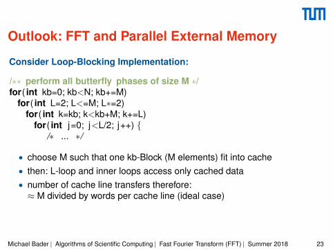
Outlook: FFT and Parallel External Memory

Consider Loop-Blocking Implementation:

/∗∗ perform all butterfly phases of size M ∗/for( int kb=0; kb<N; kb+=M)

for( int L=2; L<=M; L∗=2)for( int k=kb; k<kb+M; k+=L)

for( int j=0; j<L/2; j++) {/∗ ... ∗/

• choose M such that one kb-Block (M elements) fit into cache• then: L-loop and inner loops access only cached data• number of cache line transfers therefore:≈ M divided by words per cache line (ideal case)


Outlook: FFT and Parallel External Memory (2)

Consider Non-Blocking Implementation:

/∗∗ perform remaining butterfly levels of size L>M ∗/for( int L=2∗M; L<=N; L∗=2)


/∗ ... ∗/

• assume: N too large to fit all elements into cache• then: each L-loop will need to reload all elements X into cache• number of cache line transfers therefore:≈ M divided by words per cache line (ideal case) per L-iteration


Compute-Bound vs. Memory-Bound Performance

Consider a memory-bandwidth intensive algorithm:

• you can do a lot more flops than can be read from memory• computational intensity of a code:

number of performed flops per accessed byte

Memory-Bound Performance:

• computational intensity smaller than critical ratio• you could execute additional flops “for free”• speedup only possible by reducing memory accesses

Compute-Bound Performance:

• enough computational work to “hide” memory latency• speedup only possible by reducing operations


Outlook: The Roofline ModelG

Flo

p/s

− lo

g

Operational Intensity [Flops/Byte] − log11/21/41/8 2 4 8 16 32 64

peak stream bandwidth

without NUMA

non−unit strid

ewithout instruction−level parallism

without vectorizationS

pMV

peak FP performance

5−pt

ste

ncil

mat

rix m

ult.

(100

x100

)[Williams, Waterman, Patterson, 2008]


Outlook: The Roofline Model

Memory-Bound Performance:

• available bandwidth of a bytes per second• computational intensity small: x flops per byte• CPU thus executes x/a flops per second• linear increase of the Flop/s with variable x linear part of “roofline”• “ceilings”: memory bandwidth limited due to “bad” memory access

(strided access, non-uniform memory access, etc.)

Compute-Bound Performance:

• computational intensity small: x flops per byte• CPU executes highest possible Flop/s flat/constant “rooftop”• “ceilings”: fewer Flop/s due to “bad” instruction mix

(no vectorization, bad branch prediction, no multi-add instructions, etc.)


fast fourier transform (fft) - in.tum.de filea fast computation is possible via the...

Documents