FAKULTÄT FÜR ELEKTROTECHNIK, INFORMATIK UND MATHEMATIK

Fast Endless Polarization Control for Optical Communication Systems

Zur Erlangung des akademischen Grades

DOKTORINGENIEUR (Dr.-Ing.)

der Fakultät für Elektrotechnik, Informatik und Mathematik der Universität Paderborn

vorgelegte Dissertation von

Ariya Hidayat, M.Eng. Surabaya (Indonesien)

Referent: Prof. Dr.-Ing. Reinhold Noé Korreferent: Prof. Dr.-Ing. Rolf Schuhmann Tag der mündlichen Prüfung: 04.09.2008

Paderborn, den 15.9.2008

Diss. EIM-E/243

Abstract

Automatic endless polarization controllers are important components for polarization di-vision multiplex receivers, PMD (polarization-mode dispersion) compensators, coherentoptical receivers, optical fiber sensors and switches, as well as other optical interferomet-ric solutions. High-speed polarization changes in the transmission fibers must be tracked,without any interruption, in order to realize a near-perfect polarization matching. Thus,fast polarization controllers typically use electro-optic polarization transformers whichcurrently offer the fastest response time.

In this work, a method to characterize commercial multistage polarization transform-ers has been investigated. It has been developed based on a quaternion analysis of theoptical retarders. The polarization transformation of the retarder can be inferred ac-curately using a quaternion-based optimization on series of polarimetric measurementdata. Based on the calibration result, the electro-optic polarization transformers can becalibrated and operated as linear retarders or fractional waveplates with a high degreeof accuracy, already taking into account any of retarder’s non-ideal characteristics.

The electro-optic retarders have been used in a polarization control system. Thehardware for the system has been developed using affordable commercial off-the-shelfcomponents. The characteristics and the performance of two polarization control algo-rithms have been extensively studied. An ultra-fast implementation of the linear retarderalgorithm, running on an FPGA (field programmable gate array), has been realized andtested in a polarization tracking experiment. The retarder calibration data are storedas look-up tables for very fast access. The implementation of the control algorithm hasbeen optimized, reaching a control iteration cycle of just 2 µs. In the tracking experi-ments, it was found that the controller was able to track up to 15000 rad/s polarizationchanges caused by rotating waveplates with the maximum polarization mismatch of only0.14 rad, corresponding to a negligible intensity fluctuation of 0.02 dB. Truly endless op-eration was confirmed in a long term experiment. This polarization controller is thussuitable for polarization demultiplexing and PMD compensation.

iii

iv

Zusammenfassung

Automatische, endlose Polarisationsregelung ist ein wichtiger Bestandteil in Empfangernmit optischem Polarisationsdemultiplex, PMD-Kompensatoren (Polarisationsmodendis-persion), koharenten optischen Empfangern, faseroptischen Sensoren und Schaltern, sowiein anderen optisch interferometrischen Losungen. Schnelle Polarisationsanderungen inder Ubertragungsfaser mussen ohne Unterbrechungen nachverfolgt werden, um eine na-hezu perfekte Ubereinstimmung der Polarisationen zu erreichen. Typischerweise werdenzur Polarisationsregelung elektrooptische Polarisationstransformatoren verwendet, umkurze Reaktionszeiten zu erreichen.

In dieser Arbeit wurde eine Methode zur Charakterisierung kommerzieller, mehrstu-figer Polarisationstransformatoren auf Basis einer Quaternion-Analyse der optischenRetarder entwickelt. Die Polarisationtransformation der Retarder kann mithilfe einerQuaternion-Optimierung aus den gemessenen Polarisationsdaten gewonnen werden. Mitden Ergebnissen dieser Kalibrierung lassen sich die elektrooptischen Polarisationstrans-formatoren mit hoher Genauigkeit als lineare Retarder oder Wellenplatten betrieben,wobei die nichtidealen Charakteristiken der Retarder schon berucksichtigt werden.

Die elektrooptischen Retarder wurden in einem Polarisationregelsystem verwendet.Die Hardware dieses Systems wurde aus gunstigen, kommerziellen Standardkomponen-ten entwickelt. Die Eigenschaften und Leistungsmerkmale zweier Polarisationsregelal-gorithmen wurden ausfuhrlich untersucht. Eine sehr schnelle Implementierung einesRegelalgorithmus fur lineare Retarder wurde auf einem FPGA (field programmablegate array) realisiert und in einem Experiment uberpruft. Die Daten aus der Re-tarderkalibrierung wurden fur den schnellen Zugriff in Look-Up-Tabellen abgespeichert.Die Implementierung des Regelalgorithmus wurde optimiert und eine Ausfuhrungszeitvon nur 2 µs erreicht. Experimentell wurde herausgefunden, dass der Regler Polari-sationsanderungen, die durch rotierende Wellenplatten verursacht wurden, bis zu einerGeschwindigkeit von 15000 rad/s mit einer maximalen Polarisationsabweichung von nur0,14 Radiant, entsprechend eines geringen Intensitatsverlustes von 0,02 dB, nachver-folgen konnte. Echte endlose Regelung wurde durch ein Langzeitexperiment bestatigt.Damit erreicht dieser Polarisationsregler die Anforderungen von Polarisationsdemulti-plex und PMD-Kompensation.

v

vi

Publications

This dissertation is the result of collaborative research on the polarization aspects andadvance modulation formats in optical communications systems, which have been pub-lished in various journals and conferences. Here is a list of relevant publications withthe author’s participation.

Conference Papers

1. B. Koch, A. Hidayat, H. Zhang, V. Mirvoda, M. Lichtinger, D. Sandel, R.Noe, “12 krad/s Endless Polarization Stabilization with Lithium Niobate Com-ponent”, IEEE LEOS Summer Topical 2008, 21-23 July 2008, Acapulco, Mexico,Paper TuD2.4

2. B. Koch, A. Hidayat, H. Zhang, V. Mirvoda, M. Lichtinger, D. Sandel, R. Noe,“FPGA-basierte schnelle endlose Polarisationregelung mit Lithiumniobatbauele-ment”, 9. ITG-Fachtagung Photonische Netze, 28-29 April 2008, Leipzig, Germany

3. A. Hidayat, B. Koch, V. Mirvoda, H. Zhang, S. Bhandare, S.K. Ibrahim, D. Sandel,R. Noe, “Fast Optical Endless Polarization Tracking with LiNbO3 Component”,Optical Fiber Communication Conference (OFC 2008), 24-28 February 2008, SanDiego, USA, Paper JWA28

4. A. F. Abas, A. Hidayat, D. Sandel, S. Bhandare, R. Noe,“2.38 Tb/s (16Ö160 Gb/s)WDM Transmission over 292 km of fiber with 100 km EDFA-spacing and No Ra-man Amplification”, European Conference on Optical Communication (ECOC 2006),Cannes, France, 24-28 September 2006, Paper Tu1.5.2

5. H. Zhang, A. Fauzi Abas, A. Hidayat, D. Sandel, S. Bhandare, F. Wust, B. Milivo-jevic, R. Noe, M. Lapointe, Y. Painchaud, M. Guy, “Tunable Dispersion Compen-sation Experiment in 5.94 Tb/s WDM Transmission System”, Asia-Pacific Opti-cal Communications Conference (APOC 2005), 6–10 November 2005, Shanghai,China, Session 3a, Paper 6021-20

6. A. Hidayat, A. Fauzi Abas, D. Sandel, S. Bhandare, H. Zhang, F. Wust, B. Milivo-jevic, R. Noe, M. Lapointe, Y. Painchaud, M. Guy, “5.94 Tb/s capacity of a multi-channel tunable -700 to -1200 ps/nm dispersion compensator”, European Confer-ence on Optical Communication (ECOC 2005 ), 25-29 September 2005, Glasgow,Scotland, Paper We1.2.5

7. A. Hidayat, S. Bhandare, D. Sandel, A. Fauzi Abas, H. Zhang, B. Milivojevic,R. Noe, M. Guy, M. Lapointe, “Adaptive 700...1350 ps/nm chromatic dispersioncompensation in 1.6 Tbit/s (40Ö40 Gbit/s) DPSK and ASK transmission experi-ments over 44...81 km of SSMF”, 6. ITG-Fachtagung Photonische Netze, 2-3 May2005, Leipzig, Germany

8. B. Milivojevic, A. Fauzi Abas, A. Hidayat, S. Bhandare, D. Sandel, R. Noe,M. Guy, M. Lapointe, “160 Gbit/s, 1.6 bit/s/Hz RZ-DQPSK Polarization- Mul-tiplexed Transmission over 230 km Fiber with TDC”, European Conference on

vii

Optical Communication (ECOC 2004), September 5-9, 2004, Stockholm, Sweden,Paper We1.5.5

9. A. Fauzi Abas Ismail, D. Sandel, A. Hidayat, B. Milivojevic, S. Bhandare,H. Zhang, R. Noe, “2.56 Tbit/s, 1.6 bit/s/Hz, 40 Gbaud RZ-DQPSK polarizationdivision multiplex transmission over 273 km of fiber”, Ninth Optoelectronics andCommunications Conference/Third International Conference on Optical Internet(OECC/COIN 2004), Yokohama, Japan, July 12-16, 2004, Paper PD1-4

Journal Papers

1. A. Hidayat, B. Koch, V. Mirvoda, H. Zhang, M. Lichtinger, D. Sandel and R.Noe, “Optical 5 krad/s Endless Polarisation Tracking”, IEE Electronics Letters,Vol. 44, No. 8, pp. 546-548, 2008

2. B. Koch, A. Hidayat, H. Zhang, V. Mirvoda, M. Lichtinger, D. Sandel, R. Noe,“Optical Endless Polarization Stabilization at 9 krad/s with FPGA-Based Con-troller”, IEEE Photonics Technology Letters, Vol. 20, 2008, pp. 961-963

3. A. Hidayat, A. Fauzi Abas, D. Sandel, S. Bhandare, H. Zhang, F. Wust, B.Milivojevic, R. Noe, M. Lapointe, Y. Painchaud, M. Guy, “5.94 Tb/s (40Ö2Ö2Ö40Gbit/s) capacity of FBG-based multichannel tunable -700 to -1200 ps/nm disper-sion compensator”, Journal of Optical Communications, Vol. 27, 2006, No. 1, pp.17-19

4. A. Fauzi Abas, A. Hidayat, D. Sandel, B. Milivojevic, R. Noe, “100 km fiberspan in 292 km, 2.38 Tb/s (16Ö160 Gb/s) WDM DQPSK polarization divisionmultiplex transmission experiment without Raman amplification”, Optical FiberTechnology, 13 (2007) 46-50

5. A.F. Abas, B. Milivojevic, A. Hidayat, S. Bhandare, D. Sandel, H. Zhang, R. Noe,“2.38 Tbit/s, 1.49 bit/s/Hz (16Ö4Ö40 Gbit/s) RZ-DQPSK polarization divisionmultiplex transmission over 273 km of fiber”, Electrical Engineering, 6 July 2005

6. B. Milivojevic, A. F. Abas, A. Hidayat, S. Bhandare, D. Sandel, R. Noe, M. Guy,M. Lapointe, “1.6-bit/s/Hz, 160-Gbit/s, 230-km RZ-DQPSK Polarization Multi-plex Transmission with Tunable Dispersion Compensation”, IEEE Photonics Tech-nology Letters, Vol. 17, 2005, pp. 495-497

viii

List of Figures

2.1 Polarization ellipse . . . . . . . . . . . . . . . . . . . . . . . . . . . . . . . 42.2 Poincare sphere . . . . . . . . . . . . . . . . . . . . . . . . . . . . . . . . . 62.3 Polarization transformation as a rotation on the Poincare sphere . . . . . 72.4 Transformation of horizontal polarization by a rotatable quarter-wave plate 82.5 Transformation of elliptical polarization by a rotatable half-wave plate . . 92.6 Transformation of circular polarization by a linear retarder . . . . . . . . 102.7 Structure of an x -cut z -propagation lithium niobate retarder . . . . . . . 122.8 Polarization transformation of a lithium niobate retarder . . . . . . . . . . 122.9 Picture of EOSPACE multistage electro-optic polarization transformer . 132.10 Contour of quaternion components of a linear retarder . . . . . . . . . . . 142.11 Experiment setup for retarder characterization . . . . . . . . . . . . . . . 152.12 Characterization result of a lithium-niobate retarder . . . . . . . . . . . . 172.13 Measured output of a linear retarder with pseudo-random input pulses . . 192.14 Output of the estimated state-space model . . . . . . . . . . . . . . . . . . 192.15 Calibrated retarder voltages for different retardation and eigenmode ori-

entation . . . . . . . . . . . . . . . . . . . . . . . . . . . . . . . . . . . . . 212.16 Retarder voltages for quarter-wave plate operation . . . . . . . . . . . . . 222.17 Circular polarization transformation by a calibrated quarter-wave plate . 22

3.1 Polarization stabilization configurations . . . . . . . . . . . . . . . . . . . 243.2 Photointensity as a function of the driving signals for horizontal (left) and

+45(right) target polarization . . . . . . . . . . . . . . . . . . . . . . . . 253.3 Dithering effect at different operating points . . . . . . . . . . . . . . . . . 263.4 Contours of quaternion components of cascaded fiber squeezers . . . . . . 283.5 Worst-case tracking trajectory for a polarization controller using cascaded

fiber squeezers . . . . . . . . . . . . . . . . . . . . . . . . . . . . . . . . . 293.6 Reset scheme for the linear retarder algorithm . . . . . . . . . . . . . . . . 303.7 Transformation of a circular polarization by three fractional waveplates . 313.8 Reset scheme for the cascaded fractional waveplates algorithm . . . . . . . 343.9 Schematic diagram of the hardware . . . . . . . . . . . . . . . . . . . . . . 363.10 Picture of the controller setup . . . . . . . . . . . . . . . . . . . . . . . . . 363.11 Schematic diagram of the control software . . . . . . . . . . . . . . . . . . 373.12 Buffering to overcome SDRAM refresh . . . . . . . . . . . . . . . . . . . . 393.13 Screenshot of the status information . . . . . . . . . . . . . . . . . . . . . 393.14 Polarization scrambler using rotating waveplates . . . . . . . . . . . . . . 403.15 Distribution function (top) and complementary cumulative distribution

function (bottom) of the polarization changes . . . . . . . . . . . . . . . 413.16 Poincare sphere with scrambling up to 100 rad/s (left) and 3600 rad/s

(right) . . . . . . . . . . . . . . . . . . . . . . . . . . . . . . . . . . . . . . 413.17 Polarization tracking experiment setup with varying output polarization

(top) and varying input polarization (bottom) . . . . . . . . . . . . . . . . 423.18 Poincare sphere when controller is inactive (left) and active (right) . . . . 43

ix

3.19 Cumulative intensity distribution function during polarization trackingwith 7 µs iteration time . . . . . . . . . . . . . . . . . . . . . . . . . . . . 44

3.20 Tracking error for different polarization changes (with 7 µs control itera-tion time) . . . . . . . . . . . . . . . . . . . . . . . . . . . . . . . . . . . . 44

3.21 Cumulative intensity distribution function during polarization trackingwith 3.5 µs iteration time . . . . . . . . . . . . . . . . . . . . . . . . . . . 45

3.22 Tracking error for different polarization changes (with 3.5 µs control iter-ation time) . . . . . . . . . . . . . . . . . . . . . . . . . . . . . . . . . . . 46

3.23 Cumulative intensity distribution function during polarization trackingwith 2 µs iteration time . . . . . . . . . . . . . . . . . . . . . . . . . . . . 46

3.24 Tracking error for different polarization changes (with 2 µs control itera-tion time) . . . . . . . . . . . . . . . . . . . . . . . . . . . . . . . . . . . . 47

C.1 Setup for the WDM transmitter . . . . . . . . . . . . . . . . . . . . . . . . 56C.2 Setup for the WDM receiver . . . . . . . . . . . . . . . . . . . . . . . . . . 56C.3 Picture of the experiment setup . . . . . . . . . . . . . . . . . . . . . . . . 57C.4 Measured BER and the corresponding Q-factor as a function of frequency

for 16 channels over 273 km experiment . . . . . . . . . . . . . . . . . . . 58C.5 Measured BER and the corresponding Q-factor as a function of frequency

for 16 channels over 292 experiment . . . . . . . . . . . . . . . . . . . . . 59C.6 Measured BER and the corresponding Q-factor as a function of frequency

for 32 channels experiment . . . . . . . . . . . . . . . . . . . . . . . . . . 59C.7 Measured BER and the corresponding Q-factor as a function of frequency

for 40 channels experiment . . . . . . . . . . . . . . . . . . . . . . . . . . 60

x

Symbols and Abbreviations

Symbols

θ azimuth of polarization ellipseε ellipticity of polarization ellipseS Stokes vectorJ Jones matrixM Mueller matrixG reduced Mueller matrixΩ rotation axisϕ phase retardationψ eigenmode orientationγ fast axis angleQ quarter-wave plate quaternionH half-wave plate quaternionL linear retarder quaternionP phase shifter quaternionM mode converter quaternionC circular retarder quaternion

Abbreviations

ADC Analog-to-Digital ConverterBER Bit Error RateDAC Digital-to-Analog ConverterDPSK Differential Phase-Shift KeyingDQPSK Differential Quadrature Phase-Shift KeyingFEC Forward Error CorrectionFPGA Field Programmable Gate ArrayHWP Half-Wave PlateNRZ Non Return-to-ZeroPBS Polarization Beam SplitterPMD Polarization Mode DispersionRAM Random Access MemoryRUT Retarder Under TestRZ Return-to-ZeroSDRAM Synchronous Dynamic RAMVGA Video Graphics ArrayVHDL VHSIC Hardware Description LanguageVHSIC Very-High-Speed Integrated CircuitsWDM Wavelength-Division Multiplexing

xi

xii

Contents

Abstract iii

Zusammenfassung v

Publications vii

List of Figures x

Symbols and Abbreviations xi

Contents xiv

1 Introduction 1

2 Characterization of Electro-Optic Linear Retarders 32.1 Polarization Transformers . . . . . . . . . . . . . . . . . . . . . . . . . . . 3

2.1.1 Representations of Polarization Transformations . . . . . . . . . . 42.1.2 Optical Retarders as Polarization Transformers . . . . . . . . . . . 7

2.2 Electro-Optic Linear Retarders . . . . . . . . . . . . . . . . . . . . . . . . 112.2.1 Operating Principle . . . . . . . . . . . . . . . . . . . . . . . . . . 112.2.2 Quaternion Model . . . . . . . . . . . . . . . . . . . . . . . . . . . 132.2.3 Characterization . . . . . . . . . . . . . . . . . . . . . . . . . . . . 142.2.4 State-Space Model . . . . . . . . . . . . . . . . . . . . . . . . . . . 18

2.3 Calibrated Retarders . . . . . . . . . . . . . . . . . . . . . . . . . . . . . . 192.3.1 Linear Retarder Operation . . . . . . . . . . . . . . . . . . . . . . 202.3.2 Fractional Waveplate Operation . . . . . . . . . . . . . . . . . . . 21

3 FPGA-Based Polarization Control System 233.1 Polarization Control Algorithms . . . . . . . . . . . . . . . . . . . . . . . 23

3.1.1 Design Considerations . . . . . . . . . . . . . . . . . . . . . . . . . 253.1.2 Linear Retarder Algorithm . . . . . . . . . . . . . . . . . . . . . . 283.1.3 Cascaded Fractional Waveplates Algorithm . . . . . . . . . . . . . 30

3.2 FPGA-Based Controller Implementation . . . . . . . . . . . . . . . . . . . 353.2.1 Hardware Components . . . . . . . . . . . . . . . . . . . . . . . . . 353.2.2 Software Modules . . . . . . . . . . . . . . . . . . . . . . . . . . . . 37

3.3 Tracking Experiments . . . . . . . . . . . . . . . . . . . . . . . . . . . . . 393.3.1 Experiment Setup . . . . . . . . . . . . . . . . . . . . . . . . . . . 393.3.2 Tracking Results . . . . . . . . . . . . . . . . . . . . . . . . . . . . 42

4 Summary 49

A Basic Quaternion Algebra 51

B Non-Iterative Solutions for Absolute Orientation Problem 53

xiii

C Multichannel Polarization Division Multiplexing Transmissions 55

Bibliography 61

Acknowledgement 69

xiv

Chapter 1

Introduction

Fiber-optic communication systems are now ubiquitous in the long-haul, metro andaccess networks. The world’s current and future telecommunication structures rely onthe optical networks deployed world-wide. The increased usage and demand for Internetmultimedia rich applications certainly means a traffic growth in all network areas. Thenext generation of optical communication system is expected to fulfill this demand bypushing the performance to achieve a high capacity and highly efficient transmission.

In a wavelength-division multiplexing (WDM) system, more than one optical carrierwith different wavelengths is modulated and transmitted together in a single opticalfiber [1]. Using this technology, the transmission capacity is multiplied by the number ofthe transmitted channels. Erbium-doped fiber amplifiers (EDFA) allow all these WDMchannels to be amplified optically and thereby eliminates the need for the expensive per-channel regeneration. With a total of 273 channels, a transmission capacity of 10.92 Tb/shas been demonstrated [2].

A further increase in the transmission capacity can be reached by using spectrally-efficient modulation formats. With differential quadrature phase-shift keying (DQPSK),two bits per symbol are transmitted resulting in the doubling of the channel capac-ity [3, 4, 5]. A total capacity of 6 Tb/s in 151 DQPSK channels has been demon-strated [6]. Further capacity doubling is possible by using polarization division multi-plexing (PolDM) where two modulated signals are launched in two orthogonal polariza-tions [7, 8]. The combination of both proves to be an effective way to quadruple thebit rate [9, 10]. At 40 Gbaud, this corresponds to a 160 Gb/s channel capacity (Ap-pendix C). A record-breaking 25.6 Tb/s capacity has been reported using 160 channelsof polarization multiplexed DQPSK signals [11]. Beside the potentials, there is also abig challenge in implementing a receiver for polarization-multiplexed signals, namely toproperly perform the demultiplexing because the state of polarization of the signals likelychanges during the transmission. A fully automatic polarization demultiplexer thereforeneeds to track any polarization fluctuations in the transmission fiber, ideally fast enoughso that the two polarization channels can be demodulated properly. Crosstalk betweenthe polarization channels occurs where there is a non-negligible polarization mismatch.

Coherent optical detection is attractive due to its better sensitivity compared to thedirect detection method. In a coherent receiver, the received signal and the local oscil-lator signal are combined in an interferometer, which means that polarization matchingbetween the received signal and its local oscillator is critical [12]. One of the methods toensure polarization matching is to use a polarization controller [13] which continuouslyadjusts the polarization state of the local oscillator signal to match that of the receivedsignal. Since the received signal is subject to polarization rotations along the fiber, thespeed requirement of the controller is high because it must be capable of tracking fastpolarization changes. Even a short period of polarization mismatch may cause a loss ofdata. In addition, other optical components which rely on the interferometric method,such as fiber sensors, photonic switches, and all-optical regenerators, also have the prob-

1

lem of polarization dependence. This problem is solved either by using polarizationinsensitive devices or an automatic polarization controller.

Faster modulation techniques may bring the bit rate further towards 100 Gb/s ormore [14]. At this very high bit rate, optical signal impairment due to the polarization-mode dispersion (PMD) becomes one of the major obstacles [15, 16] and therefore ne-cessitates the use of PMD compensators. A distributed PMD compensator comprisesa number of differential group delay (DGD) sections with a polarization transformer inbetween [17]. The PMD is equalized when the PMD compensator “mirrors” the DGDvectors of the fiber. Since PMD is a stochastic phenomenon, inherently instantaneousDGD can change within a period of as short as few milliseconds to as long as a fewdays. The PMD compensator must adjust the polarization transformers to track thesechanges.

Fast, automatic endless polarization controllers are arguably important componentsfor future optical communication systems. Many polarization control experiments havebeen reported in the last two decades. Earlier experiments made use of slow mechanical(or electro-mechanical) polarization transformers which limit their actual applications.Electro-optic retardation waveplates currently offer the best response time and hencequickly become the natural choice as the control elements for fast polarization stabiliza-tion. The control algorithm is generally implemented in a digital circuit for the fastestpossible execution. Ideally the polarization controller should be as fast, if not faster,than the microsecond timescale polarization changes in the fiber trunk that have beenobserved in field trials [18, 19].

The motivation behind this work is to realize an ultra-fast automatic polarizationcontroller suitable for polarization demultiplexing and PMD compensation. For practicalreasons, the controller employs commercial electro-optic polarization transformers andother standard, off-the-shelf components. Its fast operation is achieved by implementingthe control algorithm in configurable hardware. The performance of the controller isanalyzed when it stabilizes rapidly varying random polarization states. Because it isintended to be used for polarization demultiplexing, the polarization mismatch must beas low as possible.

The rest of this dissertation is organized as follows. In Chapter 2, the working principleof the electro-optic retarder, an important control element for a fast polarization controlsystem, is described. Non-ideal characteristics of such a retarder must be analyzedand properly compensated, and a practical method to perform the characterization andcalibration is presented. In Chapter 3, a detailed mathematical analysis of importantendless polarization control algorithms is given. The architecture and implementation fora hardware-based digital controller for polarization stabilization are investigated. Theperformance of the controller is experimentally analyzed. Finally, Chapter 4 concludesthe dissertation.

2

Chapter 2

Characterization of Electro-Optic LinearRetarders

2.1 Polarization Transformers

A transverse monochromatic lightwave which propagates in the z direction, denoted asE(z, t), can be represented as the vector sum of two perpendicular fields Ex(z, t) andEy(z, t), with

Ex(z, t) = xE0,xej(ωt−kz),

Ey(z, t) = yE0,yej(ωt−kz+ϕ), (2.1)

where k is the propagation constant, ω is the frequency, and ϕ is the relative phasedifference between the fields.

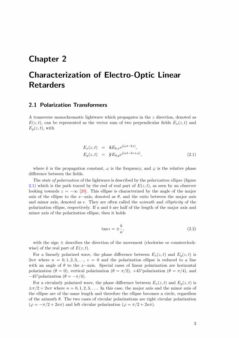
The state of polarization of the lightwave is described by the polarization ellipse (figure2.1) which is the path traced by the end of real part of E(z, t), as seen by an observerlooking towards z = −∞ [20]. This ellipse is characterized by the angle of the majoraxis of the ellipse to the x−axis, denoted as θ, and the ratio between the major axisand minor axis, denoted as ε. They are often called the azimuth and ellipticity of thepolarization ellipse, respectively. If a and b are half of the length of the major axis andminor axis of the polarization ellipse, then it holds

tan ε = ± ba, (2.2)

with the sign ± describes the direction of the movement (clockwise or counterclock-wise) of the real part of E(z, t).

For a linearly polarized wave, the phase difference between Ex(z, t) and Ey(z, t) is2nπ where n = 0, 1, 2, 3, . . ., ε = 0 and the polarization ellipse is reduced to a linewith an angle of θ to the x−axis. Special cases of linear polarization are horizontalpolarization (θ = 0), vertical polarization (θ = π/2), +45polarization (θ = π/4), and−45polarization (θ = −π/4).

For a circularly polarized wave, the phase difference between Ex(z, t) and Ey(z, t) is±π/2 + 2nπ where n = 0, 1, 2, 3, . . .. In this case, the major axis and the minor axis ofthe ellipse are of the same length and therefore the ellipse becomes a circle, regardlessof the azimuth θ. The two cases of circular polarizations are right circular polarization(ϕ = −π/2 + 2nπ) and left circular polarization (ϕ = π/2 + 2nπ).

3

Figure 2.1: Polarization ellipse

2.1.1 Representations of Polarization Transformations

Jones Vector and Stokes Vector

In equation 2.1, generally the factor ej(ωt−kz) describes the propagation of the wave andtherefore does not affect the shape of the polarization ellipse. Dropping this factor allowsthe polarization state to be represented by the Jones vector [21]

E =[E0,x(t)ejϕx

E0,y(t)ejϕy

], (2.3)

where E0,x(t) and E0,y(t) are the instantaneous scalar components of E and ϕx andϕy are the phase of each x and y components. For polarization analysis, only the relativemagnitude and phase difference between x and y components are important. The Jonesvector can be normalized by dividing it with |E| ejϕ which yields

[Ex Ey

]T with|Ex|2 + |Ey|2 = 1. Sometimes the normalized Jones vector is written with the imaginarypart of Ex chosen to be 0.

General elliptical polarization with an azimuth of θ and an ellipticity of ε can bedescribed by the normalized Jones vector [20]

E =[

cos θ cos ε+ j sin θ sin εsin θ cos ε− j cos θ sin ε

]. (2.4)

Another way to represent the state of polarization is by using the Stokes vector [22].A monochromatic lightwave with the Jones vector

[Ex Ey

]T has the correspondingStokes vector

S =

S0

S1

S2

S3

=

⟨|Ex|2 + |Ey|2

⟩⟨|Ex|2 − |Ey|2

⟩⟨2<(ExE∗y)

⟩⟨2=(ExE∗y)

⟩

, (2.5)

where 〈·〉 denotes the averaging operator. The elements S0, S1, S2, S3 are also knownas the Stokes parameters. Dividing the Stokes parameters by S0 yields the normalized

4

Stokes vector (S0 = 1 and is often dropped). Although a normalized Stokes vectorconsists of three elements, it has only two degree-of-freedom because (for fully polarizedlight) S2

1 + S22 + S2

3 = 1.General elliptical polarization with an azimuth of θ and an ellipticity of ε can be

described by the normalized Stokes vector

S =

cos 2ε cos 2θcos 2ε sin 2θ

sin 2ε

. (2.6)

Jones Matrix and Mueller Matrix

If a lightwave passes a lossless optical medium, its state of polarization may change. Thepolarization transformation can be described mathematically using Jones matrix [21] orMueller matrix [23].

Using a complex 2×2 Jones matrix J, an input polarization Ei is transformed into theoutput state Eo according to

Eo = JEi. (2.7)

If the Stokes vectors for input polarization and output polarization are denoted as Si

and So, respectively, then using a real 4×4 Mueller matrix M, the polarization trans-formation can be written as

So = MSi. (2.8)

For normalized Stokes vectors Si and So, the transformation matrix is simplified to areal 3×3 reduced Mueller matrix G, where again

So = GSi. (2.9)

If the elements of Mueller matrix M and reduced Mueller matrix G are denoted asmij (i, j = 0, 1, 2, 3) and gij (i, j = 0, 1, 2), then it holds

gij = mi+1,j+1. (2.10)

Generally, the reduced Mueller matrix G describes a rotation in the Stokes space. Foran optical medium which has an eigenmode of Ω = [ Ωx Ωy Ωz ]T and introducesphase difference of ϕ between the two transmitted eigenmodes, the reduced Muellermatrix G is obtained using Rodrigues’ rotation formula

G = I + Ω sinϕ+ Ω2(1− cosϕ), (2.11)

with

Ω =

0 −Ωz Ωy

Ωz 0 −Ωx

−Ωy Ωx 0

, (2.12)

which gives

G =

Ω2x + (Ω2

y + Ω2z) cosϕ ΩxΩy(1− cosϕ)− Ωz sinϕ ΩxΩz(1− cosϕ) + Ωy sinϕ

ΩxΩy(1− cosϕ) + Ωz sinϕ Ω2y + (Ω2

x + Ω2z) cosϕ ΩyΩz(1− cosϕ)− Ωx sinϕ

ΩxΩz(1− cosϕ)− Ωy sinϕ ΩyΩz(1− cosϕ) + Ωx sinϕ Ω2z + (Ω2

x + Ω2y) cosϕ

.(2.13)

5

Figure 2.2: Poincare sphere

For N cascaded optical medium G1,G2,G3, · · · ,GN, the total polarization transfor-mation G is

G = GN · · ·G3G2G1. (2.14)

Poincare Sphere

The three normalized Stokes parameters for an elliptical polarization with an azimuthof θ and an ellipticity of ε (equation 2.6) are the spherical coordinates of a point ina unit sphere with an azimuth of 2θ and a zenith of π/2 − 2ε [24]. The sphericalsurface occupied by elliptical polarization states is known as the Poincare sphere (figure2.2). Linear polarizations, such as horizontal polarization (H ), vertical polarization(V ), +45 polarization (P), and −45 polarization (Q), reside on the S1S2 great circle(“equator”) while circular polarizations, right (R) and left (L), reside on the intersectionsof S1S3 and S2S3 great circles (“poles”).

On the Poincare sphere, the polarization transformation by the reduced Mueller matrixG can be visualized easily because geometrically it corresponds to a rotation. Figure 2.3shows a transformation from polarization state A to B as a rotation ϕ around the axisΩ (dashed arrow) with G, ϕ, and Ω as in equation 2.11.

Quaternion

There are several ways to represent a rotation mathematically: rotation angle and axis,transformation matrix, Euler angles and Hamilton’s quaternion [25]. Throughout thisdissertation, quaternion is extensively used for rotation analysis because of its simplerepresentation and mathematical operations1. In addition, because polarization trans-

1Although, rather surprisingly, quaternion is hardly employed in literature on polarization analysis.

6

Figure 2.3: Polarization transformation as a rotation on the Poincare sphere

formation analysis is often depicted on the Poincare sphere, quaternion has also theadvantage of a direct relation to the geometrical representation of the transformation.

Generalized polarization transformation which is equivalent to a rotation of ϕ aroundthe axis Ω on the Poincare sphere can be described by the quaternion2

G = cosϕ

2+ sin

ϕ

2Ω. (2.15)

Using this quaternion, the input polarization with the normalized Stokes vector Si istransformed to the output polarization with normalized Stokes vector So according to(using equation A.13)

So = GSiG∗. (2.16)

2.1.2 Optical Retarders as Polarization Transformers

A waveplate, also known as retarder, has a fast and a slow axis. If a plane wave passesthrough a waveplate, the electrical field component along the fast axis propagates with asmaller refraction index compared to the component along the slow axis. This character-istic is known as birefringence or double refraction [26]. At the output of the waveplate,a relative phase (retardation) is introduced between the two components. It depends onthe thickness of the waveplate. In a fractional waveplate, this phase delay is set to afraction of the wavelength. The two most common fractional wave plates are quarter-wave plate and half-wave plate. If the axis of the waveplate can be freely rotated, it isoften called a rotatable waveplate.

Quarter-wave plate

In a quarter-wave plate, the phase difference is (4n + 1)π/2 with n = 0, 1, 2, ..., whichcorresponds to a delay of (4n + 1)λ/4 where λ is the wavelength. The minimum delayis thus a quarter of the wavelength, hence the name. If γ denotes the angle between thea fast axis of a rotatable quarter-wave plate and the x-component of the field, then on

2To distinguish quaternions from other symbols, quaternions are printed out in calligraphic typeface.

7

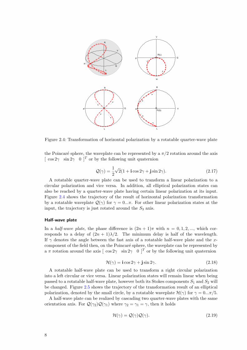
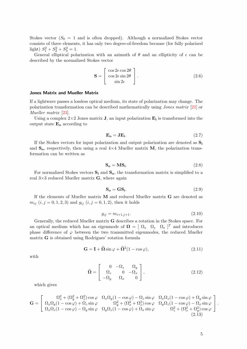
Figure 2.4: Transformation of horizontal polarization by a rotatable quarter-wave plate

the Poincare sphere, the waveplate can be represented by a π/2 rotation around the axis[ cos 2γ sin 2γ 0 ]T or by the following unit quaternion

Q(γ) =12

√2(1 + i cos 2γ + j sin 2γ). (2.17)

A rotatable quarter-wave plate can be used to transform a linear polarization to acircular polarization and vice versa. In addition, all elliptical polarization states canalso be reached by a quarter-wave plate having certain linear polarization at its input.Figure 2.4 shows the trajectory of the result of horizontal polarization transformationby a rotatable waveplate Q(γ) for γ = 0...π. For other linear polarization states at theinput, the trajectory is just rotated around the S3 axis.

Half-wave plate

In a half-wave plate, the phase difference is (2n + 1)π with n = 0, 1, 2, ..., which cor-responds to a delay of (2n + 1)λ/2. The minimum delay is half of the wavelength.If γ denotes the angle between the fast axis of a rotatable half-wave plate and the x-component of the field then, on the Poincare sphere, the waveplate can be represented bya π rotation around the axis [ cos 2γ sin 2γ 0 ]T or by the following unit quaternion

H(γ) = i cos 2γ + j sin 2γ. (2.18)

A rotatable half-wave plate can be used to transform a right circular polarizationinto a left circular or vice versa. Linear polarization states will remain linear when beingpassed to a rotatable half-wave plate, however both its Stokes components S1 and S2 willbe changed. Figure 2.5 shows the trajectory of the transformation result of an ellipticalpolarization, denoted by the small circle, by a rotatable waveplate H(γ) for γ = 0...π/5.

A half-wave plate can be realized by cascading two quarter-wave plates with the sameorientation axis. For Q(γ2)Q(γ1) where γ2 = γ1 = γ, then it holds

H(γ) = Q(γ)Q(γ). (2.19)

8

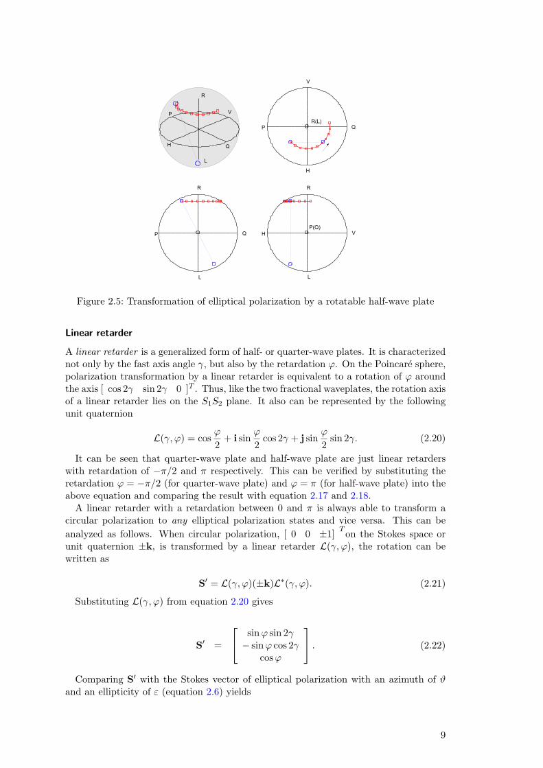
Figure 2.5: Transformation of elliptical polarization by a rotatable half-wave plate

Linear retarder

A linear retarder is a generalized form of half- or quarter-wave plates. It is characterizednot only by the fast axis angle γ, but also by the retardation ϕ. On the Poincare sphere,polarization transformation by a linear retarder is equivalent to a rotation of ϕ aroundthe axis [ cos 2γ sin 2γ 0 ]T . Thus, like the two fractional waveplates, the rotation axisof a linear retarder lies on the S1S2 plane. It also can be represented by the followingunit quaternion

L(γ, ϕ) = cosϕ

2+ i sin

ϕ

2cos 2γ + j sin

ϕ

2sin 2γ. (2.20)

It can be seen that quarter-wave plate and half-wave plate are just linear retarderswith retardation of −π/2 and π respectively. This can be verified by substituting theretardation ϕ = −π/2 (for quarter-wave plate) and ϕ = π (for half-wave plate) into theabove equation and comparing the result with equation 2.17 and 2.18.

A linear retarder with a retardation between 0 and π is always able to transform acircular polarization to any elliptical polarization states and vice versa. This can beanalyzed as follows. When circular polarization, [ 0 0 ±1] T on the Stokes space orunit quaternion ±k, is transformed by a linear retarder L(γ, ϕ), the rotation can bewritten as

S′ = L(γ, ϕ)(±k)L∗(γ, ϕ). (2.21)

Substituting L(γ, ϕ) from equation 2.20 gives

S′ =

sinϕ sin 2γ− sinϕ cos 2γ

cosϕ

. (2.22)

Comparing S′ with the Stokes vector of elliptical polarization with an azimuth of ϑand an ellipticity of ε (equation 2.6) yields

9

Figure 2.6: Transformation of circular polarization by a linear retarder

ϕ = π/2− 2ε, (2.23)γ = ±(π/2 + 2ϑ). (2.24)

On the Poincare sphere, this transformation can be easily explained. As shown in fig-ure 2.6, the axis Ω (dashed arrow) should be placed a quadrature farther than the doubleazimuth (2ϑ) of the target elliptical polarization. The amount of retardation (π/2− 2ε)corresponds to the necessary rotation (black thick arrow) to reach the target ellipticalpolarization from right circular polarization. If the input is left circular polarization,either the rotation axis must be moved additionally by π (or an odd multiple of π) orthe direction of the rotation must be reversed.

Babinet compensator [27] and Soleil-Babinet compensator [28] are other types of vari-able retarders. They are called compensators due to earlier uses to compensate the phasedelay between two field components in orthogonal polarizations. To do this, the compen-sators must be able to introduce a specific amount of positive and negative retardations.A Babinet compensator is a cascade of a linear retarder and a fractional waveplate. Thefast axis of the linear retarder is orthogonal to the fast axis of the waveplate. Whenthe retardation of the linear retarder equals that of the fractional waveplate, the totalretardation is zero. By changing the linear retarder to have a less or more retardation,the total retardation can be varied in the positive and negative range [29]. A Soleil-Babinet compensator is another variant where two linear retarders (instead of only one)are placed in front of the fractional waveplate.

Phase Shifter

A phase shifter is a special case of a linear retarder where angle γ = 0. On the Poincaresphere, polarization transformation by a phase shifter is equivalent to a rotation of ϕaround the axis S1. It can be represented by the following unit quaternion

P(ϕ) = cosϕ

2+ i sin

ϕ

2. (2.25)

10

Mode Converter

A mode converter is a special case of a linear retarder where angle γ = π/4. On thePoincare sphere, polarization transformation by a phase shifter is equivalent to a rotationof ϕ around the axis S2. It can be represented by the following unit quaternion

M(ϕ) = cosϕ

2+ j sin

ϕ

2. (2.26)

Circular Retarder

A circular retarder is a variable retarder which transforms an input polarization bya rotation around the fixed axis S3 and retardation ϕ. It can be represented by thefollowing unit quaternion

C(ϕ) = cosϕ

2+ k sin

ϕ

2. (2.27)

A circular retarder can be realized by cascading two rotatable half-wave plates. If therotations of waveplates are denoted by H(γ1) and H(γ2), then the total rotation is

H(γ2)H(γ1) = cos(π − 2γ1 − 2γ2) + k sin(π − 2γ1 − 2γ2). (2.28)

which is, according to equation 2.27, a circular retarder C(ϕ) with ϕ = 4(γ1 + γ2) .

2.2 Electro-Optic Linear Retarders

Polarization transformers can be realized by mechanical constructions which apply con-trolled changes to the properties of the fiber, for example by introducing squeezing [30] orbending [31]. However, electro-optic polarization retarder [32, 33] is currently is the mostpromising solution for a compact, reliable and responsive polarization transformer [34].In the following section, a method to characterize electro-optic polarization retardersis presented. Using the characterization result, it is possible to find the polarizationtransformation of the device as a function of applied electrode voltages with a very highdegree of accuracy.

2.2.1 Operating Principle

The electro-optic polarization transformer using LiNbO3 (lithium niobate) crystals isshown in figure 2.7 [32]. It comprises of z -propagated waveguide on an x -cut substratewith three symmetrical electrodes (V1, V2, and V3). If the middle electrode is grounded(V3 = 0), the horizontal field component Ey in the region of the waveguide is inducedby V1 − V2, while the vertical field component Ex is induced by V1 + V2.

The polarization transformation of the device depicted on the Poincare sphere is shownin figure 2.8. Its phase retardation ϕ and eigenmode orientation ψ are determined by

ϕ ∼√E2x + E2

y , (2.29a)

tan(ψ − π/2) ∼ ExEy

. (2.29b)

The polarization transformer is thus a linear retarder. The eigenmode of the device liesin the S1S2 plane. From equation 2.29b, it can be seen that the eigenmode is endlessly

11

Figure 2.7: Structure of an x -cut z -propagation lithium niobate retarder

Figure 2.8: Polarization transformation of a lithium niobate retarder

12

Figure 2.9: Picture of EOSPACE multistage electro-optic polarization transformer

rotated even with a limited range of V1, V2. A circular polarization at the input ofthe device can be transformed into any elliptical polarization provided that V1, V2 canintroduce a retardation in the range of 0...π.

Several stages of electro-optic polarization transformer can be cascaded. Figure 2.9shows a picture of a commercial electro-optic polarization transformer from EOSPACEwhich consists of 8 cascaded stages with a total insertion loss of < 3 dB.

2.2.2 Quaternion Model

A model of electro-optic polarization transformer can be used to determine its operationas a function of electrode voltages, as well as to identify the electrode voltages neededto achieve a specific polarization conversion [35]. Polarization transformation of anyretarders can be represented by a quaternion and thus, the model that is presented hereis basically the quaternion model as a function of the applied voltages.

Based on equations 2.29a and 2.29b, suppose that:

Ex = κx(V1 + V2 − Vo,x),Ey = κy(−V1 + V2 − Vo,y),

ϕ =π

Vπ

√E2x + E2

y .

,

then it follows

cosψ =κx(V1 + V2 − Vo,x)√

κ2x(V1 + V2 − Vo,x)2 + κ2

y(−V1 + V2 − Vo,y)2, (2.30a)

sinψ =κy(−V1 + V2 − Vo,y)√

κ2x(V1 + V2−Vo,x)2 + κ2

y(−V1 + V2 − Vo,y)2, (2.30b)

ϕ =π

Vπ

√κ2x(V1 + V2 − Vo,x)2 + κ2

y(−V1 + V2 − Vo,y)2. (2.30c)

The quaternion model of a linear retarder is thus

13

L(V1, V2) = cosπ

2Vπ

√κ2x(V1 + V2 − Vo,x)2 + κ2

y(−V1 + V2 − Vo,y)2 +

(iκx(V1 + V2 − Vo,x)√

κ2x(V1 + V2 − Vo,x)2 + κ2

y(−V1 + V2 − Vo,y)2+

jκy(−V1 + V2 − Vo,y)√

κ2x(V1 + V2 − Vo,x)2 + κ2

y(−V1 + V2 − Vo,y)2) ·

sinπ

2Vπ

√κ2x(V1 + V2 − Vo,x)2 + κ2

y(−V1 + V2 − Vo,y)2 (2.31)

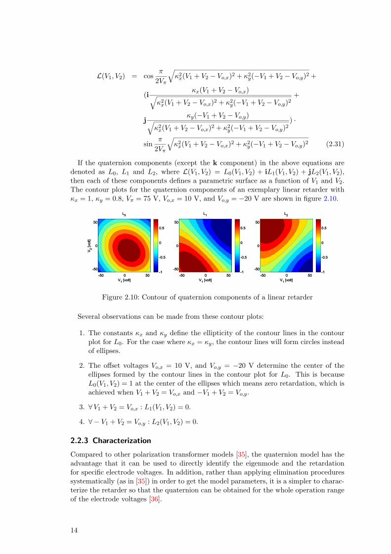
If the quaternion components (except the k component) in the above equations aredenoted as L0, L1 and L2, where L(V1, V2) = L0(V1, V2) + iL1(V1, V2) + jL2(V1, V2),then each of these components defines a parametric surface as a function of V1 and V2.The contour plots for the quaternion components of an exemplary linear retarder withκx = 1, κy = 0.8, Vπ = 75 V, Vo,x = 10 V, and Vo,y = −20 V are shown in figure 2.10.

Figure 2.10: Contour of quaternion components of a linear retarder

Several observations can be made from these contour plots:

1. The constants κx and κy define the ellipticity of the contour lines in the contourplot for L0. For the case where κx = κy, the contour lines will form circles insteadof ellipses.

2. The offset voltages Vo,x = 10 V, and Vo,y = −20 V determine the center of theellipses formed by the contour lines in the contour plot for L0. This is becauseL0(V1, V2) = 1 at the center of the ellipses which means zero retardation, which isachieved when V1 + V2 = Vo,x and −V1 + V2 = Vo,y.

3. ∀V1 + V2 = Vo,x : L1(V1, V2) = 0.

4. ∀ − V1 + V2 = Vo,y : L2(V1, V2) = 0.

2.2.3 Characterization

Compared to other polarization transformer models [35], the quaternion model has theadvantage that it can be used to directly identify the eigenmode and the retardationfor specific electrode voltages. In addition, rather than applying elimination proceduressystematically (as in [35]) in order to get the model parameters, it is a simpler to charac-terize the retarder so that the quaternion can be obtained for the whole operation rangeof the electrode voltages [36].

14

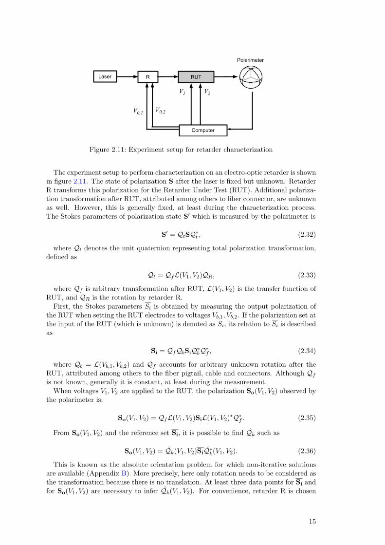
Figure 2.11: Experiment setup for retarder characterization

The experiment setup to perform characterization on an electro-optic retarder is shownin figure 2.11. The state of polarization S after the laser is fixed but unknown. RetarderR transforms this polarization for the Retarder Under Test (RUT). Additional polariza-tion transformation after RUT, attributed among others to fiber connector, are unknownas well. However, this is generally fixed, at least during the characterization process.The Stokes parameters of polarization state S′ which is measured by the polarimeter is

S′ = QtSQ∗t , (2.32)

where Qt denotes the unit quaternion representing total polarization transformation,defined as

Qt = QfL(V1, V2)QR, (2.33)

where Qf is arbitrary transformation after RUT, L(V1, V2) is the transfer function ofRUT, and QR is the rotation by retarder R.

First, the Stokes parameters Si is obtained by measuring the output polarization ofthe RUT when setting the RUT electrodes to voltages Vb,1, Vb,2. If the polarization set atthe input of the RUT (which is unknown) is denoted as Si, its relation to Si is describedas

Si = QfQbSiQ∗bQ∗f , (2.34)

where Qb = L(Vb,1, Vb,2) and Qf accounts for arbitrary unknown rotation after theRUT, attributed among others to the fiber pigtail, cable and connectors. Although Qfis not known, generally it is constant, at least during the measurement.

When voltages V1, V2 are applied to the RUT, the polarization So(V1, V2) observed bythe polarimeter is:

So(V1, V2) = QfL(V1, V2)SiL(V1, V2)∗Q∗f . (2.35)

From So(V1, V2) and the reference set Si, it is possible to find Qk such as

So(V1, V2) = Qk(V1, V2)SiQ∗k(V1, V2). (2.36)

This is known as the absolute orientation problem for which non-iterative solutionsare available (Appendix B). More precisely, here only rotation needs to be considered asthe transformation because there is no translation. At least three data points for Si andfor So(V1, V2) are necessary to infer Qk(V1, V2). For convenience, retarder R is chosen

15

to be another electro-optic retarder so that different Si and So(V1, V2) are obtained bychanging the electrode voltages V0,1, V0,2 applied to R.

Eliminating Si gives an alternative expression for So(V1, V2)

So(V1, V2) = Qk(V1, V2)QfQbSiQ∗bQ∗f Q∗k(V1, V2). (2.37)

Comparing the above equation with equation 2.35 gives

QfL(V1, V2)SiL(V1, V2)∗Q∗f = Qk(V1, V2)QfQbSiQ∗bQ∗f Q∗k(V1, V2), (2.38)

which is simplified to

QfL(V1, V2) = Qk(V1, V2)QfQb. (2.39)

Solving for L(V1, V2) yields

L(V1, V2) = Q−1f Qk(V1, V2)QfQb. (2.40)

If the voltages Vb,1, Vb,2 are chosen so that Qb = L(Vb,1, Vb,2) = 1, then the aboveequation is simplified to

L(V1, V2) = Q−1f Qk(V1, V2)Qf . (2.41)

which means that L(V1, V2) is just Qk(V1, V2) with its coordinate system rotated byQ−1f . Arbitrary constant rotation of the coordinate system like this typically can be

ignored. However, it is useful to choose an estimate of Qf so that L(V1, V2) is as closeas possible to the birefringence model of a linear retarder (equation 2.31), since thecharacterized device is a linear retarder anyway. If the estimates of Qf and L(V1, V2)are denoted as Qf and L(V1, V2) respectively, then it follows

L(V1, V2) = Q−1f Qk(V1, V2)Qf . (2.42)

Because Qf ,Qk, and L(V1, V2) are all quaternions, they can be written as

Qf = Qf,0 + iQf,1 + jQf,2 + kQf,3,

Qk(V1, V2) = Qk,0(V1, V2) + iQk,1(V1, V2) + jQk,2(V1, V2) + kQk,3(V1, V2),

L(V1, V2) = L0(V1, V2) + iL1(V1, V2) + jL2(V1, V2) + kL3(V1, V2), (2.43)

then using equation 2.42, the i, j, and k components of L(V1, V2) are

L1(V1, V2) = Qk,1(V1, V2)(Q2f,0 + Q2

f,1 − Q2f,2 − Q2

f,3) +

Qk,2(V1, V2)(2Qf,0Qf,3 + 2Qf,1Qf,2) +

Qk,3(V1, V2)(2Qf,1Qf,3 − 2Qf,0Qf,2), (2.44a)

L2(V1, V2) = Qk,1(V1, V2)(2Qf,1Qf,2 − 2Qf,0Qf,3) +

Qk,2(V1, V2)(Q2f,0 − Q2

f,1 + Q2f,2 − Q2

f,3) +

Qk,3(V1, V2)(2Qf,0Qf,1 + 2Qf,2Qf,3), (2.44b)

L3(V1, V2) = Qk,1(V1, V2)(2Qf,1Qf,3 + 2Qf,2Qf,0) +

Qk,2(V1, V2)(2Qf,2Qf,3 − 2Qf,1Qf,0) +

Qk,3(V1, V2)(Q2f,0 − Q2

f,1 − Q2f,2 + Q2

f,3), (2.44c)

16

L0 L1

L2 L3

Figure 2.12: Characterization result of a lithium-niobate retarder

To have L(V1, V2) as a linear retarder, Qf must be chosen so that the characteristicsof the components L(V1, V2) match those of a linear retarder, based on observations offigure 2.10 described previously.

By defining a cost function J(Qf ) as

J(Qf ) =∑i

L21(Vb,1 + i, Vb,2 − i) +∑

i

L22(Vb,1 + i, Vb,2 + i) +∑

i

∑j

L23(Vi, Vj), (2.45)

then Qf can be obtained using iterative multidimensional optimization with J(Qf )as the minimization criteria. For this particular optimization problem, particle swarmoptimization algorithm [37] was found to give accurate solutions with a satisfactoryconvergence speed.

Figure 2.12 shows the characterization result of a lithium-niobate electro-optic re-tarder. The electrode voltages are swept over the range (−56V, 56V ) with a voltagequantization of 3.75V . It was found that Vb,1 = 1.73V and Vb,2 = −1.39V . The charac-terization result matches with the birefringence model shown previously in figure 2.10.As can be seen from the contour plot of L3, the k component of L(V1, V2) is not com-pletely zero. However it is very close to zero especially in the vicinity of the centers ofthe ellipses formed by the contour lines of L1 where the retardation is small.

17

2.2.4 State-Space Model

The response of an x -cut, z -propagated waveguide lithium-niobate linear retarder isincreased by a finite buffer layer isolation [34]. The retarder therefore does not givefully instantaneous response. If such a retarder is employed in an automatic polarizationcontrol system, this non-rectangular step response may limit the tracking speed [38]. Itis thus interesting to analyze the transient-stage retarder response in order to find thelimitation of its operation in a polarization controller.

From the quaternion model of an electro-optic linear retarder, the retardation ϕ can bedescribed (using the time-invariant state-space form [39]) by the following linear system

dx(t)dt

= Ax(t) + B[V1(t) V2(t)

], (2.46a)

ϕ(t) = Cx(t), (2.46b)

where x(t) is the state vector, A is the state matrix, B is the input matrix and C isthe output matrix.

The linear retarder can be operated with V1 = V2 (only the field component Ex isapplied) or V1 = −V2 (only the field component Ey is applied), where it acts like a modeconverter and a phase shifter, respectively [40]. Without a loss of generality, here onlythe case V3 = 0 is considered. The state-space model is thus simplified and discretizedto

x1(k + 1) = A1x1(k) + B1V1(k), (2.47a)ϕ1(k) = C1x1(k). (2.47b)

The model parameters A1, B1, and C1 can be estimated by system identificationmethods [41]. It is common to measure the input and output sequences of the systemexperimentally and then optimize the model parameters to fit the model’s dynamic tothe observations.

For this analysis, a pseudo-random binary sequence (PRBS) with the shortest pulsewidth of 1 ms as the input excitation V1(t) was used to trigger the retarder and thenϕ1(t) was recorded with a sampling rate of 10 MHz. The result is shown in figure 2.13where the dotted line and the solid line denote the retarder input voltage and normalizedoutput retardation, respectively. In this figure, the response is shown only for about 30ms, although it was actually measured and further analyzed for a duration of up to 250ms.

From the measurement data, the N4SID subspace identification algorithm [42, 43] wasused to estimate the model parameters. The discrete state-space model was specified fora sampling period of 10 µs and an order of 4. The optimal parameters were found as

A1 =

0.1349 −0.5721 0.5607 0.2577−0.1765 0.8701 0.6144 0.1723

0.0112 0.0091 0.8156 −0.39290.0002 0 −0.0296 −0.3524

, (2.48a)

B1 =

−0.8563−0.1739

0.01150.0019

, (2.48b)

C1 =[−0.9773 −0.2111 0.0177 0.0001

]. (2.48c)

18

0 5 10 15 20 25 30

0

0.2

0.4

0.6

0.8

1

Time [ms]

Out

put [

a.u]

Input Output

Figure 2.13: Measured output of a linear retarder with pseudo-random input pulses

0 5 10 15 20 25 30

0

0.2

0.4

0.6

0.8

1

Time [ms]

Out

put [

a.u]

Figure 2.14: Output of the estimated state-space model

Figure 2.14 shows the response of the estimated model, which is similar to the actualretarder response shown in figure 2.13. Although the model is only of the fourth order,the estimation error already reaches a mean and a standard deviation of 7.16 · 10−3 and4.36 · 10−3, respectively. A more accurate estimation, if necessary, can be obtained byincreasing the order of the state-space model.

It has been suggested that the response of the electro-optic can be improved by elec-trical equalization [38]. The state-space model that is presented here could be used tosynthesize an equalizer if this were necessary.

2.3 Calibrated Retarders

Using the quaternion model of a linear retarder (equation 2.20), the necessary voltageswhich correspond to a specific retardation and eigenmode can be calculated. Graphically,this is also clear from the contour plots of the quaternion components of the linearretarder (figure 2.10 and 2.12). For example, since a contour line in the contour plot forL0 is the locus for constant retardation, voltages that trace along this contour line rotate

19

the eigenmode and thus operate the linear retarder like a rotating fractional waveplate.

2.3.1 Linear Retarder Operation

For an ideal linear retarder, the voltages which correspond to a certain rotation arefunctions of the model parameters (κx, κy, Vπ, Vo,x, and Vo,y). For an electro-opticlinear retarder that has been characterized, these voltages can be inferred from thecharacterization result. This can be formulated as follows. The unit quaternion of thecharacterized linear retarder for electrode voltages V1, V2 must represent a retardationof ϕ and the eigenmode of [ cosψ sinψ 0 ]T , written as

L(V1, V2) = cosϕ

2+ i sin

ϕ

2cosψ + j sin

ϕ

2sinψ. (2.49)

L(V1, V2) is obtained from the optimization process in the characterization procedure(equation 2.42). However, L(V1, V2) is not a continuous two-dimensional function of theelectrode voltages V1, V2 since V1, V2 are swept with a quantization of 3.75V . If thereexist integer values i1, i2, j1, j2 such as i1∆V < V1 < i2∆V and j1∆V < V2 < j2∆Vwhere ∆V denotes the voltage quantization, then L(V1, V2) can be approximated bytwo-dimensional spherical linear interpolation (equation A.17) using the following set ofequations:

L(V1, j1∆V ) =sin(i2 − V1/∆V )δ1

sin δ1L(i1∆V, j1∆V ) +

sin(V1/∆V − i1)δ1sin δ1

L(i2∆V, j1∆V ), (2.50a)

L(V1, j2∆V ) =sin(i2 − V1/∆V )δ2

sin δ2L(i1∆V, j2∆V ) +

sin(V1/∆V − i1)δ2sin δ2

L(i2∆V, j2∆V ), (2.50b)

L(V1, V2) =sin(j2 − V2/∆V )δ

sin δL(V1, j1∆V ) +

sin(V2/∆V − j1)δsin δ

L(V1, j2∆V ), (2.50c)

with

cos δ1 = L(i1∆V, j1∆V ) · L(i2∆V, j1∆V ), (2.51a)cos δ2 = L(i1∆V, j2∆V ) · L(i2∆V, j2∆V ), (2.51b)cos δ = L(V1, j1∆V ) · L(V1, j2∆V ). (2.51c)

By defining a cost function

J(V1, V2) = [L(V1, V2)−

(cosϕ

2+ i sin

ϕ

2cosψ + j sin

ϕ

2sinψ)]2, (2.52)

V1, V2 can be obtained using two-dimensional optimization steps with J(V1, V2) as theminimization criteria. With V1, V2 for a given rotation (retardation ϕ and eigenmodeorientation ψ) obtained from the characterization result, it is then possible to operate

20

−30

−20

−10

0

10

20

0

0.5

1

1.5

0

2

4

6

8−40

−20

0

20

40

φψ

V1

−20

−15

−10

−5

0

5

10

15

20

25

0

0.5

1

1.5

0

2

4

6

8−40

−20

0

20

40

φψ

V2

Figure 2.15: Calibrated retarder voltages for different retardation and eigenmodeorientation

the electro-optic retarder to realize a specific polarization transformation. This is alsosufficiently true even if the retarder inhibits a somewhat non-ideal behavior. Thus, usingthese steps it can be said that the retarder is calibrated.

Figure 2.15 shows the surface plots of the voltages V1, V2 as functions of retardationϕ (0 . . . π/2) and eigenmode orientation ψ (0 . . . 2π) obtained using the above optimiza-tion procedure for the electro-optic linear retarder for which the characterization resultis already shown in figure 2.12.

2.3.2 Fractional Waveplate Operation

To operate a linear retarder as a quarter-wave plate, the retardation ϕ is simply setto π/2. This means, the cost function J(V1, V2) for the optimization procedure to findV1, V2 is simplified to

J(V1, V2) = [L(V1, V2)− 12

√2(1− i cosψ − j sinψ)]2. (2.53)

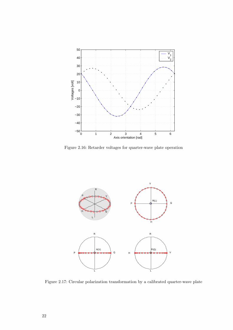
Figure 2.16 shows voltages V1, V2 for 32 different quarter-wave plate axis orientationsψ (0 . . . π) again for the electro-optic linear retarder for which the characterization re-sult is already shown in figure 2.12. If the quaternions L(V1, V2) for the different axisorientation are used to transform a circular polarization, the result will be linear po-larizations, as shown on the Poincare sphere in figure 2.17. The resulting polarizationstates mismatch between the transformed trajectory and linear polarization states has aroot mean square error of only 0.0176. It proves that V1, V2 in figure 2.16 really operatethe calibrated linear retarder as a quarter-wave plate with a high degree of accuracy.

For half-wave plate operation, the voltages will be suitably doubled because now theretardation ϕ equals π.

21

0 1 2 3 4 5 6−50

−40

−30

−20

−10

0

10

20

30

40

50

Axis orientation [rad]

Vol

tage

s [v

olt]

V1

V2

Figure 2.16: Retarder voltages for quarter-wave plate operation

Figure 2.17: Circular polarization transformation by a calibrated quarter-wave plate

22

Chapter 3

FPGA-Based Polarization Control System

3.1 Polarization Control Algorithms

An automatic polarization controller has the task of transforming an input state ofpolarization into an output state of polarization subject to certain conditions. In asystem where the optical signal needs to be coupled into a polarization sensitive device,the polarization controller must perform the polarization transformation so that theoutput polarization always matches the required polarization state for the device. If theinput polarization is time-variant, this implies a polarization tracking since the necessarypolarization transformation is also time-variant. This holds also for a varying outputpolarization state. Thus, a common structure to implement an automatic polarizationcontroller is a feedback control system.

An early application of automatic polarization control is for optical coherent receivers.In such a receiver, the received signal and the local oscillator signal are combined in aninterferometer and then detected with a photo detector. The photo intensity is

I ∝ cos2(ϕ/2), (3.1)

where ϕ denotes the angle (on the Poincare sphere) between the polarization stateof the received signal and the polarization state of the local oscillator. The intensityvanishes when the polarization states are orthogonal (ϕ = π). Maximum intensity isobtained only when ϕ = 0 which occurs only when both polarization states matchperfectly. Intensity optimization can be achieved by using a polarization controller forthe local oscillator signal so that its polarization state match that of the received signal.However, the polarization state of the received signal continuously changes due to thetemperature, vibration and other mechanical disturbances on the transmission fiber andtherefore necessitates the use of automatic polarization control.

The first attempts at polarization stabilization used a polarimeter to give a feedbacksignal to the polarization transformer [44, 45]. The polarimeter measured the currentpolarization state and delivered two error signals corresponding to the amount of re-tardation corrections required to bring the input polarization to the target output po-larization. Two independent proportional-integral controllers were driven by the errorsignals in order to adjust the retardation of the two waveplates. Because a polarimeteris needed, it can not be used in a system where the output polarization can not bemeasured or is not available, for example in a coherent receiver. However, this can beeasily remedied since the intensity detected by the receiver (equation 3.1) serves as thefeedback signal [46, 47]. When this feedback signal is maximized, it indicates matchedpolarization states.

Other common polarization stabilization configurations are illustrated in figure 3.1. Avarying input polarization is to be stabilized into a fixed output polarization, for exampleif the signal is to be processed further by a polarization sensitive device. A polarizer

23

Figure 3.1: Polarization stabilization configurations

which passes only one polarization state (which matches its transmission axis) can beused to get a fixed polarization optical signal. The intensity at its output depends on thepolarization matching similar to the relation in equation 3.1 but now with ϕ denotingthe angle between the input polarization state and the polarizer axis. If the intensity ismaximized by the controller, the output of the polarizer will have a fixed polarization anda maximum optical intensity. Another variant is by using a polarization beam splitterthat outputs two orthogonal polarizations. In this configuration, the intensity at one ofits output should be minimized so that the other output will have a maximum opticalintensity.

In a polarization division multiplex transmission, two modulated data streams in twoorthogonal polarizations are launched into the transmission fiber. At the receiver, thetwo polarizations stay generally orthogonal. However, their absolute polarization statesare unknown due to random polarization changes in the fiber. A receiver must thereforedemultiplex the signal into two polarization channels before the data stream in each ofthe channel can be correctly demodulated. Usually a setup similar to figure 3.1 (bottom)is implemented, but with both outputs of the polarization beam splitter connected to thesubsequent demodulation circuit. In addition, since both polarization channels containdata, the feedback signal can not continue to be obtained anymore from a simple photodetector at only one optical output of the beam splitter. One solution is to electricallymix the demodulated electrical signal and recovered clock and use the result as thefeedback signal since it is proportional to the optical intensity of the selected polarizationchannel [48]. Another alternatives is to use correlation signal or interference signalbetween the two polarization channels, each being inversely related to the degree ofpolarization matching in the beam splitter [49, 50].

24

3.1.1 Design Considerations

Polarization Transformers

An important factor that determines the performance of an automatic polarization con-troller is the speed of the polarization transformer that is used as the control element.In its early development, fiber squeezers with electromechanical driving were commonchoices [44, 47, 51, 52]. A fiber squeezer can be treated as a retardation waveplatewith a fixed eigenmode and a variable retardation. Therefore a cascade of few fibersqueezers (with unequal eigenmodes) is necessary to realize an arbitrary polarizationtransformation. The same principle can be applied to electro-optic polarization trans-formers with fixed axes [45, 53, 54] which can operate at a higher speed compared tothe fiber squeezers. Rotating fractional waveplates implemented as electro-optic devices[55], liquid crystals [56, 57, 58] or magnetic Faraday rotators [59, 60] can also be usedas the polarization transformers. Nowadays, commercial automatic polarization con-trollers typically use electro-optic polarization transformers [61, 62] because currentlyelectro-optic devices offer the fastest response time.

Figure 3.2 shows the photointensity in equation 3.1 as a function of polarization trans-fomer driving signals, if the polarization transfomer has a circular polarization at itsinput and the target polarization is horizontal (left) or +45(right). Since this intensityis related to the polarization matching, the controller generally dithers or modulates thedriving signals and detects the changes in the feedback signal to infer the degree of polar-ization state matching [63], similar to the principle of a lock-in amplifier. The amount ofdithering must be chosen to be small enough so that it does not introduce considerablesignal fluctuation but at the same time large enough so that the corresponding changesin the feedback signal is still not submerged in noises. Figure 3.3 illustrates the differentchanges in the feedback signal I(α) as a function of the operating point α when thelow-amplitude parasitic modulation is applied to α at different points. The controlleressentially obtains ∂I(α)/∂α (positive at point P, negative at point R) and uses it toapply the necessary correction to bring α to the optimal value (point Q). Since only(instantaneous) ∂I(α)/∂α is important, not the absolute value of I(α), the controllertolerates slow fluctuations of the intensity.

−50

0

50

−50

0

500

0.5

1

V1 [volt]V2 [volt]

−50

0

50

−50

0

500

0.5

1

V1 [volt]V2 [volt]

Figure 3.2: Photointensity as a function of the driving signals for horizontal (left) and+45(right) target polarization

25

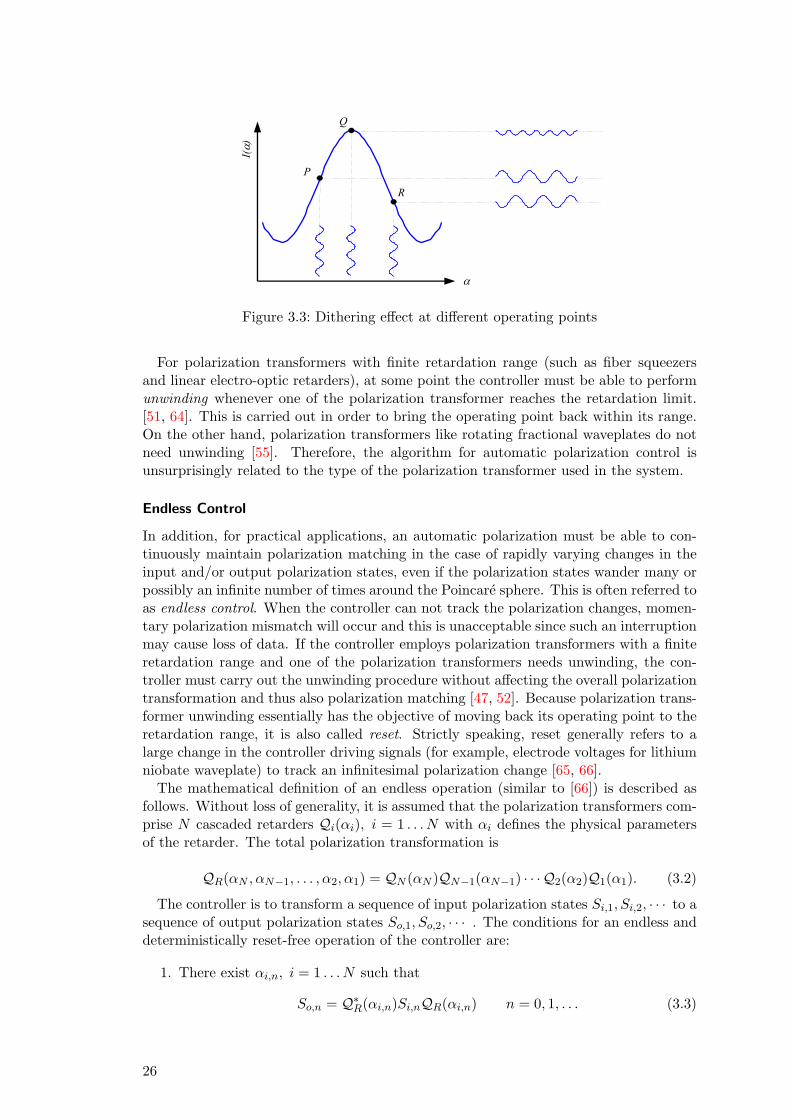
Figure 3.3: Dithering effect at different operating points

For polarization transformers with finite retardation range (such as fiber squeezersand linear electro-optic retarders), at some point the controller must be able to performunwinding whenever one of the polarization transformer reaches the retardation limit.[51, 64]. This is carried out in order to bring the operating point back within its range.On the other hand, polarization transformers like rotating fractional waveplates do notneed unwinding [55]. Therefore, the algorithm for automatic polarization control isunsurprisingly related to the type of the polarization transformer used in the system.

Endless Control

In addition, for practical applications, an automatic polarization must be able to con-tinuously maintain polarization matching in the case of rapidly varying changes in theinput and/or output polarization states, even if the polarization states wander many orpossibly an infinite number of times around the Poincare sphere. This is often referred toas endless control. When the controller can not track the polarization changes, momen-tary polarization mismatch will occur and this is unacceptable since such an interruptionmay cause loss of data. If the controller employs polarization transformers with a finiteretardation range and one of the polarization transformers needs unwinding, the con-troller must carry out the unwinding procedure without affecting the overall polarizationtransformation and thus also polarization matching [47, 52]. Because polarization trans-former unwinding essentially has the objective of moving back its operating point to theretardation range, it is also called reset. Strictly speaking, reset generally refers to alarge change in the controller driving signals (for example, electrode voltages for lithiumniobate waveplate) to track an infinitesimal polarization change [65, 66].

The mathematical definition of an endless operation (similar to [66]) is described asfollows. Without loss of generality, it is assumed that the polarization transformers com-prise N cascaded retarders Qi(αi), i = 1 . . . N with αi defines the physical parametersof the retarder. The total polarization transformation is

QR(αN , αN−1, . . . , α2, α1) = QN (αN )QN−1(αN−1) · · · Q2(α2)Q1(α1). (3.2)

The controller is to transform a sequence of input polarization states Si,1, Si,2, · · · to asequence of output polarization states So,1, So,2, · · · . The conditions for an endless anddeterministically reset-free operation of the controller are:

1. There exist αi,n, i = 1 . . . N such that

So,n = Q∗R(αi,n)Si,nQR(αi,n) n = 0, 1, . . . (3.3)

26

2. Parameters αi,n always lie within the operating limitations of the retarders

3. There is an absolute constant 0 < CQ <∞ such that

maxi=1...N

|αi,n − αi,n−1| ≤ CQ(‖Si,n − Si,n−1‖+ ‖So,n − So,n−1‖) n > 0. (3.4)

The last condition guarantees that the changes in the physical parameters of the po-larization transformers when the controller responds to a certain change in the inputand/or output polarization will be well defined within a certain limit. The controller iscalled reset-free only when this condition is fulfilled.

Tracking Speed Limit

To judge the performance of an automatic polarization control system, it is necessaryto know its worst-case tracking speed. Because the polarization transformer has limitedresponse time, the theoretical tracking speed limit can be analyzed by finding one ormore sequences in the input and/or output polarization states that put the highest loadon the controller. Put another way, the worst-case sequence causes the controller tooperate on its limit which mathematically means that maxi=1...N |αi,n − αi,n−1| reachesits maximum value.

Assume the polarization transformer is a cascade of two fiber squeezers 1. The axesof the fiber squeezers are inclined by π/4 rad to each other, this is equivalent to π/2distance between the eigenmodes on the Poincare sphere. The arrangement can also bethought as a combination of a phase shifter P(VP ) followed by a mode converterM(VM )with (according to equation 2.25 and 2.26)

P(VP ) = cos12VPVP,π

+ i sin12VPVP,π

, (3.5a)

M(VM ) = cos12VMVM,π

+ j sin12VMVM,π

, (3.5b)

where VP , VM are the normalized driving signals for the fiber squeezers and VP,π, VM,π

are the driving signals for π retardation. The total polarization transformation is

Q(VP , VM ) = M(VM )P(VP )

= cos12VMVM,π

cos12VPVP,π

+ i cos12VMVM,π

sin12VPVP,π

+

j sin12VMVM,π

cos12VPVP,π

− k sin12VMVM,π

sin12VPVP,π

. (3.6)

For ease of visualization, the quaternion components in the above equations aredenoted as Q0, Q1, Q2 and Q3, where Q(VP , VM ) = Q0(VP , VM ) + iQ1(VP , VM ) +jQ2(VP , VM ) + kQ3(VP , VM ). The contour plots for these quaternion components areshown in figure 3.4 with VP , VM in the operation range of 1 . . . 3, corresponding to aretardation range (of the mode converter and phase shifter) of π . . . 3π.

From the contour plot of Q0, it is obvious that VP = 2, VM = 2 is the “center point”,any contour lines will circle this center point. The contour line with the longest perimeter

1Two fiber squeezers do not permit endless control, this arrangement is only given as an illustration.

27

−1

−0.5

0

0.5

1 2 31

1.5

2

2.5

3

Q0

VP

−1

−0.5

0

0.5

1 2 31

1.5

2

2.5

3

Q1

−1

−0.5

0

0.5

1 2 31

1.5

2

2.5

3

Q2

VM

VP

−1

−0.5

0

0.5

1 2 31

1.5

2

2.5

3

Q3

VM

Figure 3.4: Contours of quaternion components of cascaded fiber squeezers

is Q0 = 0 which is along the border of the contour plot. This particular contour line canalso be specified by the parametric equation (t = 0 . . . 1)

VP (t) = 2 + (1− |4t|+ |4t− 1|+ |4t− 2| − |4t− 3|), (3.7a)VM (t) = 2 + (1− |4t− 1|+ |4t− 2|+ |4t− 3| − |4t− 4|). (3.7b)

This polarization transformer is then used in an automatic polarization control systemwhere the input polarization state is circular. The driving signals VP (t), VM (t) accordingto the above equation will transform the circular input polarization into a trajectoryR− V −L−H −R−P −L−Q−R as depicted in figure 3.5. If this trajectory is to betracked by the controller (and assuming that the controller can track it perfectly), thenit is the worst-case polarization state sequence for this type of polarization transformersince the accumulated driving signals (on the voltage plane VP ,VM ) reach the maximumvalue.

3.1.2 Linear Retarder Algorithm

A linear retarder, as described in subsection 2.1.2, has two parameters: the axis angle γand the retardation ϕ. When using Poincare sphere analysis, the double azimuth angleψ is often used instead of the axis angle γ, with ψ = 2γ. The unit quaternion thatrepresents a linear retarder is

L(ψ,ϕ) = cosϕ

2+ i sin

ϕ

2cosψ + j sin

ϕ

2sinψ. (3.8)

Operation Principle

For polarization stabilization where either the input polarization or output polarizationis fixed, a linear retarder is a natural choice for the polarization transformer. As showngeometrically in figure 2.6, a linear retarder with a retardation between 0 and π is

28

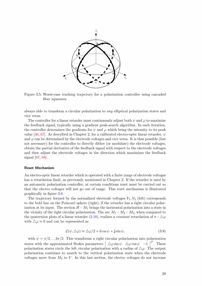
Figure 3.5: Worst-case tracking trajectory for a polarization controller using cascadedfiber squeezers

always able to transform a circular polarization to any elliptical polarization states andvice versa.

The controller for a linear retarder must continuously adjust both ψ and ϕ to maximizethe feedback signal, typically using a gradient peak-search algorithm. In each iteration,the controller determines the gradients for ψ and ϕ which bring the intensity to its peakvalue [40, 67]. As described in Chapter 2, for a calibrated electro-optic linear retarder, ψand ϕ can be determined by the electrode voltages and vice versa. It is thus possible (butnot necessary) for the controller to directly dither (or modulate) the electrode voltages,obtain the partial derivative of the feedback signal with respect to the electrode voltagesand then adjust the electrode voltages in the direction which maximizes the feedbacksignal [67, 68].

Reset Mechanism

An electro-optic linear retarder which is operated with a finite range of electrode voltageshas a retardation limit, as previously mentioned in Chapter 2. If the retarder is used byan automatic polarization controller, at certain conditions reset must be carried out sothat the electro voltages will not go out of range. This reset mechanism is illustratedgraphically in figure 3.6.

The trajectory formed by the normalized electrode voltages V1, V2 (left) correspondsto the bold line on the Poincare sphere (right), if the retarder has a right circular polar-ization at its input. The section H−M1 brings the horizontal polarization into a state inthe vicinity of the right circular polarization. The arc M1−M2−M3, when compared tothe quaternion plots of a linear retarder (2.10), realizes a constant retardation of π−4ϕwith 4ϕ ≈ 0 and can be represented as

L(ψ,4ϕ) ≈ 4ϕ/2 + i cosψ + j sinψ, (3.9)

with ψ = π/2 . . . 3π/2. This transforms a right circular polarization into polarizationstates with the approximated Stokes parameters

[4ϕ sinψ 4ϕ cosψ −1

]T . Thesepolarization states circle the left circular polarization with a radius of 4ϕ. The outputpolarization continues to march to the vertical polarization state when the electrodevoltages move from M3 to V . In this last section, the electro voltages do not increase

29

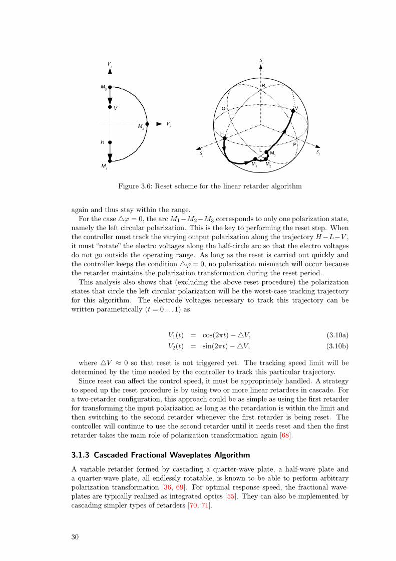
Figure 3.6: Reset scheme for the linear retarder algorithm

again and thus stay within the range.For the case4ϕ = 0, the arc M1−M2−M3 corresponds to only one polarization state,

namely the left circular polarization. This is the key to performing the reset step. Whenthe controller must track the varying output polarization along the trajectory H−L−V ,it must “rotate” the electro voltages along the half-circle arc so that the electro voltagesdo not go outside the operating range. As long as the reset is carried out quickly andthe controller keeps the condition 4ϕ = 0, no polarization mismatch will occur becausethe retarder maintains the polarization transformation during the reset period.

This analysis also shows that (excluding the above reset procedure) the polarizationstates that circle the left circular polarization will be the worst-case tracking trajectoryfor this algorithm. The electrode voltages necessary to track this trajectory can bewritten parametrically (t = 0 . . . 1) as

V1(t) = cos(2πt)−4V, (3.10a)V2(t) = sin(2πt)−4V, (3.10b)

where 4V ≈ 0 so that reset is not triggered yet. The tracking speed limit will bedetermined by the time needed by the controller to track this particular trajectory.

Since reset can affect the control speed, it must be appropriately handled. A strategyto speed up the reset procedure is by using two or more linear retarders in cascade. Fora two-retarder configuration, this approach could be as simple as using the first retarderfor transforming the input polarization as long as the retardation is within the limit andthen switching to the second retarder whenever the first retarder is being reset. Thecontroller will continue to use the second retarder until it needs reset and then the firstretarder takes the main role of polarization transformation again [68].

3.1.3 Cascaded Fractional Waveplates Algorithm

A variable retarder formed by cascading a quarter-wave plate, a half-wave plate anda quarter-wave plate, all endlessly rotatable, is known to be able to perform arbitrarypolarization transformation [36, 69]. For optimal response speed, the fractional wave-plates are typically realized as integrated optics [55]. They can also be implemented bycascading simpler types of retarders [70, 71].

30

Figure 3.7: Transformation of a circular polarization by three fractional waveplates

Operation Principle

If each waveplate is independently adjustable, it gives a total number of three degree-of-freedom. Transformation from a static, arbitrary polarization into another static,arbitrary polarization however can be specified using only two degree-of-freedom, forexample a rotation axis for a fixed non-zero rotation angle. Thus, there are many possiblecombinations of the waveplate orientations that correspond to a specific polarizationtransformation. The easiest is as follows: the first quarter-wave plate transforms theelliptical input polarization into a linear polarization, the half-wave plate rotates thislinear polarization along the S1S2 great circle so that it can be transformed by the lastquarter-wave plate to reach the target polarization.

If the rotations of the first quarter-wave plate, the half-wave plate and the secondquarter-wave plate are denoted as Q(γ1), H(γ2), and Q(γ3), respectively, then based onequation 2.17 and 2.18, the total transformation is

R(γ1, γ2, γ3) = Q(γ3)H(γ2)Q(γ1). (3.11)

Straightforward but lengthy quaternion multiplications yield

R(γ1, γ2, γ3) = i(cos 2γ2 − cos(2γ1 − 2γ2 + 2γ3))/2 +j(sin 2γ2 − sin(2γ1 − 2γ2 + 2γ3))/2 +k(sin(2γ1 − 2γ2) + sin(2γ2 − 2γ3))/2 +(− cos(2γ3 − 2γ2)− cos(2γ2 − 2γ1))/2. (3.12)

Figure 3.7 shows an example of the polarization transformation by the waveplatesQ(γ1), H(γ2), Q(γ3), with γ1 = π, γ2 = 11π/32, and γ3 = 0.

In some experiments, the last quarter-wave plate is rotated synchronously with thefirst quarter-wave plate so that γ3 = γ1 + π/2 [72, 73]. The whole arrangement nowhas only two degree-of-freedom. In this case, the total transformation of the cascadedwave-plates is simplified to

R(γ1, γ2) = i cos(2γ2 − 2γ1) cos 2γ1 +j cos(2γ2 − 2γ1) sin 2γ1 +−k sin(2γ2 − 2γ1). (3.13)

31

The above unit quaternion represents a rotation of ϕ around the axis Ω according to

ϕ = π, (3.14a)

Ω =

cos(2γ2 − 2γ1) cos 2γ1

cos(2γ2 − 2γ1) sin 2γ1

− sin(2γ2 − 2γ1)

. (3.14b)

The retarder acts like a generalized half-wave plate. Its rotation axis Ω is endlesslyrotatable. It depends on γ1, γ2 which do not have any limit and hence require no un-winding.

In another experiment, the quarter-wave plates are rotated simultaneously so thatγ3 = γ1 [69]. This simplifies the total transformation of the cascaded wave-plates to

R(γ1, γ2) = i sin(2γ2 − 2γ1) sin 2γ1 +j sin(2γ2 − 2γ1) cos 2γ1 −cos(2γ2 − 2γ1). (3.15)

The above unit quaternion represents a rotation of ϕ around the axis Ω according to

ϕ = 2π − (4γ1 − 4γ2), (3.16a)

Ω =

sin 2γ1

− cos 2γ1

0

. (3.16b)

Here, the retarder acts like a linear retarder with endlessly rotatable eigenmode. Theretardation is adjustable via γ1, γ2 in the whole range of 0 . . . 2π.

When the retarder is used in a polarization control system, each waveplate is typicallyadjusted independently, either by an analog lock-in amplifier [72] or a digital feedbackcontroller [73, 69], to maximize (or minimize) the feedback signal. The digital controlleris preferred because it is much faster than the analog counterpart.

Simplification for Polarization Tracking with Fixed Input

For polarization tracking with either a fixed input polarization or a fixed output polar-ization, two quarter-wave plates are sufficient to perform the necessary endless transfor-mation. For example, a quarter-wave plate followed by a half-wave plate can transforma varying input polarization into a fixed linear output polarization [46, 74]. Here it isshown that with a circular input polarization, an arbitrary output polarization can bereached by a cascade of only two quarter-wave plates. Transformation of a circular po-larization by a quarter-wave plate and a half-wave plate is always a linear polarization,described as

H(γ2)Q(γ1)kQ∗(γ1)H∗(γ2) =

− sin(4γ2 − 2γ1)cos(4γ2 − 2γ1)

0

. (3.17)

Therefore, the cascaded waveplates H(γ2)Q(γ1) can be replaced by just a singlequarter-wave plate Q(γ1) where

32

γ1 = π + 2γ2 − γ1. (3.18)

The arrangement Q(γ1), H(γ2), and Q(γ3) is now simplified to Q(γ1) and Q(γ3) only.The total transformation is

R(γ1, γ3) =12− 1

2cos(2γ1 − 2γ3) +

12i(cos 2γ1 − cos 2γ3) +

12j(sin 2γ1 − sin 2γ3) +

12k sin(2γ1 − 2γ3). (3.19)

Controller Dead Lock

The use of fractional waveplates with one control loop for each waveplate however presenta practical problem. There are always polarization states where the feedback signal isinsensitive or less sensitive to the dithering of one control variable [75]. Such polarizationstates are often called “dead spots”.

For the retarder as described by equation 3.13, when γ2 = γ1 −4γ/2 with 4γ ≈ 0,the transformation of the retarder is approximated as

R(γ2, dγ) ≈ i cos 2γ2 + j sin2γ2 + k4γ. (3.20)

The rotation axis of the retarder lies on the S1S2 great circle, its azimuth depends onγ2 . A right circular polarization is rotated by the retarder to

R(γ2,4γ)kR∗(γ2,4γ) =

24γ cos 2γ2

24γ sin 2γ2

4γ2 − 1

. (3.21)

It is very close to the left circular polarization. The controller is to track an ellipticalpolarization with azimuth θ = 0 and ellipticity ε = −π/4+4ε/2 with 4ε ≈ 0, which hasthe corresponding (approximated) Stokes vector

[4ε 0 4ε2/2− 1

]T . The feedbacksignal is thus

I(γ2) = (1 +[4ε 0 4ε2/2− 1

] 24γ cos 2γ2

24γ sin 2γ2

4γ2 − 1

)/2

= 1 +4ε4γ cos 2γ2 + (4ε24γ2/2−4γ2 −4ε2/2)/2. (3.22)

Dithering the orientation axis of the half-wave plate (γ2, together with γ1) has thepurpose of getting the derivative of the feedback signal with respect to γ2. This can befound from the above equation as

∂I(γ2)∂γ2

= − 4ε4γ sin 2γ2. (3.23)

In this case, because 4γ ≈ 0 and 4ε ≈ 0, dithering γ2 produced very little change inthe feedback signal which possibly can not be detected properly by the electronic circuit.In addition, the controller may cease to work (“dead lock”) as ∂I(γ2)/∂γ2 approacheszero. The worst case is when γ2 is orthogonal to the optimal orientation axis but can notbe corrected by the controller because the factor sin 2γ2 vanishes and ∂I(γ2)/∂γ2 = 0.

33

Figure 3.8: Reset scheme for the cascaded fractional waveplates algorithm

Reset Mechanism

The arrangement of fractional waveplates is often claimed to be reset-free [69, 72, 73].This stems from the fact that not a single waveplate needs any unwinding. However, ac-cording to the definition of reset described previously, the algorithm that uses this wave-plates arrangement is not necessarily reset-free [38, 65]. Abrupt changes in waveplatesparameters are still possible under certain circumstances. One example is illustratedgraphically in figure 3.8. The trajectory formed by the retarder parameters γ1, γ2 (left)corresponds to the bold line on the Poincare sphere (right), if the waveplates has a leftcircular polarization at its input and γ3 = γ1 +π/2. When the controller must track thevarying output polarization along the trajectory H−R−V and initially γ1 = 0, γ2=7π/4,it must rapidly change γ2 by π/2 just when the output polarization passes the right cir-cular. This proves that the waveplates arrangement is not reset-free. It could be shownthat the same condition applies for the simplified arrangement of waveplates as describedin equation 3.19.

For the case γ3 = γ1, the retarder becomes a linear retarder (equation 3.15). Therefore,it subjects to the same limitation and reset mechanism as in the linear retarder algorithm.Again, it means that this arrangement of waveplates (γ3 = γ1) is also not reset-free.

Tracking Speed Limit

For the case γ3 = γ1 + π/2, reset is necessary when the input polarization needs to berotated into target polarization states in the vicinity of its orthogonal. Without lossof generality, the input polarization can be assumed to be right circular and the targetpolarization states reside on a very small circle with a radius of 4ε ≈ 0 centered at theleft circular polarization. Such polarization states have an ellipticity ε = −π/4 +4ε/2and can be represented by the Stokes vector

[4ε cosα 4ε sinα 4ε2/2− 1

]T for α =0 . . . 2π. For the retarder as described in equation 3.20, at the points where 4ε/2 ≈ 4γ,the optimal control variables should be set to

γ1 ≈ α/2, (3.24a)γ2 ≈ α/2. (3.24b)

The controller must rotate γ1, γ2 in the range of 0 . . . π for α = 0 . . . 2π. As shown inthe previous chapter, rotating the axis of a calibrated electro-optic quarter-wave plate

34

by π (by 2π on the Poincare sphere) means driving the electrode voltages up to ±30V .For a half-wave plate, the necessary driving voltages are doubled. This is the case evenfor an infinitesimal 4ε. A similar problem arises for γ3 = γ1 configuration.

3.2 FPGA-Based Controller Implementation

Because of their complexity, polarization control algorithms are typically implementedin digital circuits. There have been reports on digital realization of polarization sta-bilization using a microprocessor [67], a combination of basic digital blocks [73] and adedicated digital signal processor [61]. In this dissertation, an implementation of polar-ization control algorithm in a field programmable gate array (FPGA) is described. AnFPGA is chosen because it allows a very fast execution of the control algorithm. Inaddition, it also offers a high degree of parallelism, a feature which can be utilized toimplement the tracking algorithm efficiently.

3.2.1 Hardware Components

Several hardware components are needed to implement a polarization controller digi-tally. The feedback signal (that is, the photo intensity) must be detected by a photodetection circuit and then converted using an analog-to-digital converter (ADC) to thediscrete binary representation. The driving signal from the controller must be convertedusing a digital-to-analog converter (DAC) so that it can drive the lithium-niobate lin-ear retarder. For faster operation, more than one retarder is used and therefore severalDACs are required. For an ultra-fast polarization tracking, the conversion speed and theperformance of the ADC and the DACs play an important role.

The controller is implemented in a Xilinx Spartan-3 XC3S1000 FPGA [76]. It com-prises 1920 configurable logic blocks (CLBs). One block has 8 logic cells, each cell canbe flexibly programmed to perform combinational and sequential logic. In total, thelogic capability of the Spartan-3 XC3S1000 is equivalent to approximately a millionlogic gates. For a limited amount of data storage, the Spartan-3 also offers two typesof random access memory (RAM): distributed RAM [77] and block RAM [78]. In aSpartan-3 XC3S1000 chip, up to 120 Kbits of distributed RAM and 432 Kbits of blockRAM are available. In addition, Spartan-3 XC3S1000 has 24 dedicated single-cycle 18-bithardware multipliers [79] which are useful to carry out complicated calculations.

For development convenience, a prototyping board XSA-3S1000 [80] is used. Theprototyping board is equipped with a Spartan-3 XC3S1000 FPGA and two externalmemory chips: 32 Mbyte synchronous dynamic RAM (Samsung K4S561632ETC75 [81])and 2 MB Flash RAM (Spansion S29AL016M10TAI020[82, 83]). A video connector anda parallel port are also available on the prototyping board.

The setup for the hardware of the polarization controller is shown schematically infigure 3.9. The ADC and the DACs are connected to the input/output pins of theSpartan-3 FPGA. For troubleshooting and debugging, a video graphics array (VGA)monitor and a computer (or a notebook) are connected to the XSA-3S1000 board throughthe video connector and parallel port, respectively. The monitor is used to displaythe status of the controller wheres the computer is important to retrieve additionalinformation and changing the operation of the controller.

The hardware of this polarization controller consists of affordable commercial, off-the-shelf components only. This reduces both the development time and cost. Figure 3.10shows the picture of the actual controller setup.

35

Figure 3.9: Schematic diagram of the hardware

Figure 3.10: Picture of the controller setup

36

Figure 3.11: Schematic diagram of the control software

3.2.2 Software Modules

The polarization stabilization is implemented in software running on the Spartan-3FPGA. Figure 3.11 shows the simplified architecture of the software. It is designedto be modular for ease of development and maintenance. Hardware interfacing to theADC, the DACs and VGA monitor are separated into different modules which allowsabstractions and simplification of the main program. Each module is programmed inVHDL (VHSIC2 hardware description language).

Gradient Descent Controller

The controller implements the linear retarder algorithm (subsection 3.1.2). For thegradient descent method, the controller dithers the driving signals (electrode voltages ofthe retarders) and measures the intensity to infer the gradient. To reach a maximumperformance, the code to perform the gradient algorithm is optimized to get the shortestpossible execution time and thus is clocked at 50 MHz (20 ns cycle period). As the result,one control iteration can be carried out in just 7 µs. A later improved version of thecode even cuts the iteration time down to 3.5 µs. An even more optimized version bringsthe iteration time to only 2 µs. This corresponds to polarization tracking up to 140000iterations/second, 285000 iterations/second, and 500000 iterations/second, respectively.Each iteration is designed to correct ≤1 rad of polarization mismatch.

Look-Up Tables

The electro-optic linear retarders used in the controller are characterized and calibratedusing the method described in Chapter 2. The calibration data are important for thecontroller since it allows the control algorithm to treat the utilized retarders as one ideallinear retarder. In this implementation, the calibration data are stored in the memory,not hard-coded in the program. It makes it easy to substitute the electro-optic retarderswithout the need to modify the program. Because of the size of the data, the programmakes use of all types of memory available on the prototyping board: Flash, SDRAM,Block RAM. Flash is important because it is non-volatile and hence it retains the writtendata even when the system is not powered. SDRAM is slow but it has a big capacity,whereas Block RAM can store only a very limited amount of data but is neverthelessvery fast. A combination of these three memory types allows the controller to managethe calibration data effectively.

2Very-High-Speed Integrated Circuits

37

The calibration data is stored in the form of look-up tables [84]. Because the memorycapacity is finite, each look-up table has a coarse resolution (granularity). A fast two-dimensional interpolation is carried out to improve the accuracy. For a two dimensionalfunction f(x, y), the look-up table is in the form of f(xn, yn) where xn, yn = 1, 2, 3, ...Nand the linear interpolation is

f(x, y) ≈ (1− y + yn)(1− x+ xn)f(xn, yn) +(1− y + yn)(x− xn)f(xn + 1, yn) +(y − yn)(1− x+ xn)f(xn, yn + 1) +(y − yn)(x− xn)f(xn + 1, yn + 1), (3.25)

with xn ≤ x < xn + 1 and yn ≤ y < yn + 1. If xu = x − xn and because xn is aninteger, xu is simply the fractional part of x. If xv = 1 − x + xn, then xv is obtainedby using the relation xu + xv = 1. Thus, this approximation is implemented by usingthe most significant bits of x, y as indices to the table and the rest of the bits for theinterpolation.

A less accurate but faster version

f(x, y) ≈ f(xn, yn) + (x− xn)∂f(x, y)∂x

+ (y − yn)∂f(x, y)∂y

, (3.26)

where ∂f(x, y)/∂x, ∂f(x, y)/∂y are precomputed off-line, is also used under certaincircumstances.

Photointensity Analysis

The photodetection circuit and the corresponding ADC deliver the feedback signal to thecontrol algorithm. To reduce the effect of the measurement noise, the ADC is clocked ata frequency 50 MHz that is faster than the dithering in the gradient descent controller.The measured photointensity is downsampled before being processed by the controller.

To analyze the tracking performance of the controller, the photointensity is analyzedin a histogram module. The histogram module counts the “occurrences” for variousphotointensities. The result can be retrieved from a computer/notebook. If this is carriedout during a continuous polarization tracking, the amount of polarization mismatch canbe concluded by the probability density function of the intensity.

For the characterization purpose (as described in subsection 2.2.4), it is necessaryto record the photointensity at the highest possible sampling frequency. When this isperformed for a duration of several milliseconds, the amount of the sampled data is quitelarge. Thus, the data can be saved only to the SDRAM which has a massive total capacityof 32 MB. This however presents a challenge because the SDRAM can not continuouslybe written due to its intermittent refresh procedure. The refresh of the SDRAM can beas long as 120 ns and occurs at least every 8 µs. The solution is to use a cache buffer [85]between the ADC and the SDRAM, as depicted in figure 3.12. The RAM controlleralways tries to fill the SDRAM as fast as possible but whenever the SDRAM is in the“busy” state (while performing the refresh), the samples are temporarily stored in thebuffer. This buffer will be quickly emptied as soon as the SDRAM finishes with therefresh. This caching technique allows storing the photointensity (from the ADC) to theSDRAM at a constant rate of up to 25 MHz.

38

Figure 3.12: Buffering to overcome SDRAM refresh

Figure 3.13: Screenshot of the status information

Troubleshooting

Two means for troubleshooting are built in the control program: remote debugging andstatus information. For remote debugging, the program can communicate to a client toolrunning on a computer/notebook connected to the controller hardware using a parallelport. This is useful in the early stage of development, for example to verify the resultof the calculation performed on the FPGA (programmed in VHDL) and compare itagainst the reference version (written as MATLAB script). Data transfer is done using acompact and error-tolerant protocol. However, the speed is limited by the parallel portinterface so it does not permit real-time monitoring.

To display the important status of the controller, a video controller module has beendeveloped. This module sends VGA-compatible signals to an external monitor. Thephotointensity and the electrode voltages of the retarders can be observed on the monitor,as shown in figure 3.13.

3.3 Tracking Experiments

3.3.1 Experiment Setup

The speed of a polarization controller can be objectively measured when the controlleris stabilizing rapidly varying polarization states. Random changes to polarization stateare possible to realize by passing a fixed polarization through a polarization scrambler.

Figure 3.14 shows the structure of a simple polarization scrambler using cascadedrotating fractional waveplates. The quarter-wave plates were made from endlessly ro-tatable fiber loops. A stepper motor was used to drive each fiber loop, the speed anddirection were determined by the microcontroller-based driving circuit. The quarter-wave plates run at different rates between –6 Hz and +6 Hz. The half-wave plate wasmade from a commercial bulk optic waveplate and rotated by a DC motor. It can reacha maximum speed of 23000 rotations per minute.

The maximal polarization rotation speed is obtained when a linear polarization passesthe half-wave plate. Without loss of generality, assuming this linear polarization is a

39

Figure 3.14: Polarization scrambler using rotating waveplates

horizontal polarization, after rotated by the half-wave plate it becomes (obtained usingequation 2.18)

H(γ)iH∗(γ) =

cos 4γsin 4γ

0

. (3.27)

Within one revolution of the half-wave plate, γ changes from 0 to 2π and the horizontalinput polarization is transformed into a linear polarization that traces the S1S2 greatcircle (on the Poincare sphere) with an azimuth angle from 0 to 4(2π). This means, whenthe half-wave plate is rotated at the rate of 280 Hz, it causes a maximal polarizationchange of 7000 rad/s on the Poincare sphere. Practically, the polarization change doesnot always reach the maximal speed at all times since the polarization state at the inputof the half-wave plate is not always linear. The quarter-wave plates in front of thehalf-wave plate distribute the polarization states on the Poincare sphere and thus varythe total polarization rotation speed. The additional quarter-wave plates after the half-wave plate ensure that the rotation trajectories seen by the polarization controller arerandomly reoriented. Figure 3.15 shows the result of the rotating waveplates simulation.The polarization changes distribution function (top) and its complementary cumulativedistribution function (bottom) indicate that the mean of the polarization changes isindeed about 5500 rad/s and most of the time almost maximum polarization changesare generated by rotating waveplates.

Figure 3.16 shows the scrambling result on the Poincare sphere, taken with a polarime-ter in a time period of 5 minutes. With polarization changes up to 100 rad/s (left), thetrajectories are still visible. However, with very fast scrambling up to 3600 rad/s (right),the Poincare sphere is filled only with points because the sampling rate of the polarime-ter is too slow compared to the scrambling speed. This validates the operation of thepolarization scrambler.

The performance of the polarization controller was analyzed using the setup shown infigure 3.17 (top). An optical signal from a laser at 1551 nm was passed through thepolarizer, the polarization controller and then the polarization scrambler. The feedbacksignal for the controller was obtained after the polarization beam splitter (PBS) and anoptical attenuator. The controller was set to minimize this feedback signal. Here a PBSwas used instead of a polarizer so that the maximized optical signal was available at theother output of the PBS as well. The attenuator was inserted because the photodetectorcircuit was able to work with a maximum of -11 dB optical power. Instead of an atten-uator, an optical coupler (5% or 10%) could also be used if both outputs of the PBS areneeded, for example in a polarization demultiplex system.

To verify the gradient algorithm in the digital controller, first the scrambler was turnedoff and its waveplates were manually adjusted until a maximum feedback signal wasobtained. The output of the PBS was connected to a polarimeter for monitoring purpose.The polarization controller was deliberately modified until its control speed was only oneiteration per second. The controller was then enabled and it automatically transformed

40

0 1000 2000 3000 4000 5000 6000 70000

0.5

1

1.5

2x 10

7N

umbe

r of

hits

0 1000 2000 3000 4000 5000 6000 70000

0.5

1

Cum

ulat

ive

prob

abili

ty

Polarization changes [rad/s]

Figure 3.15: Distribution function (top) and complementary cumulative distributionfunction (bottom) of the polarization changes

Figure 3.16: Poincare sphere with scrambling up to 100 rad/s (left) and 3600 rad/s(right)

41

Figure 3.17: Polarization tracking experiment setup with varying output polarization(top) and varying input polarization (bottom)

the polarization until the feedback signal reached its minimum point. Due to the slowcontrol speed of the controller, the changes of the control voltages could be observedclearly and this is used to confirm the tracking of the controller [84].

The controller was brought back to its maximum control speed. The scrambler wasswitched on and set to produce polarization rotation up to 3600 rad/s on the Poincaresphere. The performance of the controller was checked on the polarimeter. Figure 3.18shows the difference in the polarization changes on Poincare sphere when the controlleris inactive (left) and active (right), taken in a time period of 5 minutes. Without anycontrol, the Poincare sphere was randomly filled with points. With automatic control,the polarization states were successfully confined in a circle with an approximate radiusof only 0.1 rad.

The experiment setup was modified to check the controller for stabilizing a varyingoutput polarization, as in figure 3.17 (bottom). With polarization scrambling and activecontrol, essentially identical result was obtained. That is, the stabilized polarizationstates were within a 0.1 rad radius circle on the Poincare sphere.

3.3.2 Tracking Results

The experiment setup was used to test the performance of the FPGA-based polarizationcontroller, for the “slow” version (7 µs iteration time), the “fast” version (3.5 µs iterationtime), and the “ultrafast” version (2 µs iteration time), for different scrambling speeds.The maximum tracking error could not be determined using the polarimeter because thepolarimeter was too slow to catch the fastest glitches. Therefore, the feedback signalreceived by the digital controller was recorded every 1.4 µs and then analyzed. Foreach scrambling configuration, the intensity analysis was carried out for a 30 minutes’continuous tracking. The maximum tracking speed was determined by the scrambling

42

Figure 3.18: Poincare sphere when controller is inactive (left) and active (right)

speed for which the intensity error did not exceed 1%.

5000 rad/s Tracking Experiment [86, 87]

With 7 µs control iteration time, the test was conducted with a rotation rate of thehalf-wave plate up to 200 Hz. Figure 3.19 shows the cumulative density function F (I)of the intensity, that is, the time-averaged probability that the intensity becomes worsethan the value given in the abscissa. The intensity measurement error was not excluded,as shown by the reference measurement without light (optical signal), which indicatedthat the true results were likely to be better. For a half-wave plate (HWP) rotation rateof 200 Hz (polarization changes up to 5000 rad/s), the controller was able to performtracking with a maximum intensity error of <1%. The probability that the intensity errorwas larger than 0.73% was only 1%. Even with a half-wave plate rotation rate of 280Hz (polarization changes up to 5000 rad/s) the controller can still perform the trackingalthough the maximum intensity error >1% was reached. In figure 3.20, the intensityerror (right scale) and the corresponding calculated polarization error (left scale) aredisplayed as a function of the maximum polarization changes. The mean polarizationerror was always <0.063 rad. At 5000 rad/s, the maximum polarization and intensityerrors were 0.17 rad and 0.73%, respectively. For the maximized signal exiting at theother PBS output, this corresponds to a loss of −10 · log(1− (< 0.0073)) =< 0.032 dB.

9000 rad/s Tracking Experiment [88]

A faster version of the software, with 3.5 µs iteration time, was also tested using theexperiment setup. Since now the controller is twice as fast, the maximum rotation rateof the half-wave plate was doubled as well.

Figure 3.21 shows the cumulative density function F (I). For a half-wave rotationof 360 Hz (polarization changes up to 9000 rad/s), the controller was able to performtracking with a maximum intensity error of <0.5%. The probability that the intensityerror was larger than 0.25% was only 1%. In figure 3.22, the intensity error (rightscale) and the corresponding calculated polarization error (left scale) are displayed as afunction of the maximum polarization changes. The mean polarization error was always< 0.06 rad. At 9000 rad/s, the maximum polarization and intensity errors were 0.13 radand 0.43%, respectively. For the maximized signal exiting at the other PBS output, this

43

Figure 3.19: Cumulative intensity distribution function during polarization tracking with7 µs iteration time

Figure 3.20: Tracking error for different polarization changes (with 7 µs control iterationtime)

44

Figure 3.21: Cumulative intensity distribution function during polarization tracking with3.5 µs iteration time

corresponds to a loss of −10 · log(1− (< 0.0043)) =< 0.019 dB.

15000 rad/s Tracking Experiment [89]

The fastest version of the software, with only 2 µs iteration time, was tested usingthe experiment setup. The maximum rotation rate of the half-wave plate was suitableincreased to 600 Hz.

Figure 3.23 shows the cumulative density function F (I). For a half-wave rotation of600 Hz (polarization changes up to 15000 rad/s), again the controller was able to per-form tracking with a maximum intensity error of <0.5%. During this 30-minute period,the total accumulated polarization changes is > 20 Mrad. Figure 3.22 shows the inten-sity error (right scale) and the corresponding calculated polarization error (left scale)displayed as a function of the maximum polarization changes. The mean polarizationerror was always < 0.061 rad. At 15000 rad/s, the maximum polarization and intensityerrors were 0.14 rad and 0.48%, respectively. For the maximized signal exiting at theother PBS output, this corresponds to a loss of −10 · log(1− (< 0.0048)) =< 0.021 dB.

45

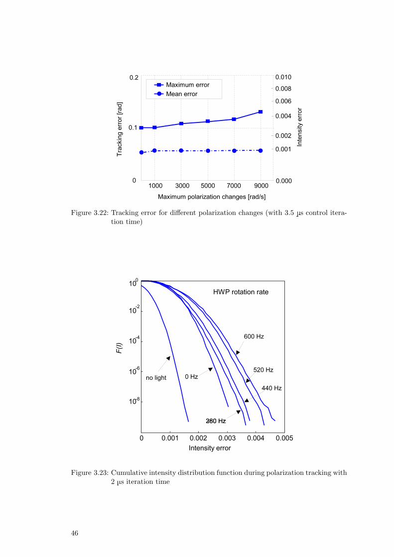
Figure 3.22: Tracking error for different polarization changes (with 3.5 µs control itera-tion time)

Figure 3.23: Cumulative intensity distribution function during polarization tracking with2 µs iteration time

46

Figure 3.24: Tracking error for different polarization changes (with 2 µs control iterationtime)

47

48

Chapter 4

Summary

An ultra-fast automatic polarization controller designed for polarization demultiplex-ing and PMD compensation has been developed in this work. The controller employscommercial electro-optic retarders, runs on an FPGA, tracks the polarization changesendlessly and reaches the control speed of 15000 rad/s.

Retarder Characterization

In Chapter 2, the operating principle of optical retarders is analyzed using quaternionalgebra. Specifically, a quaternion model for an electro-optic lithium niobate linearretarder is then formulated. Since commercial retarders might exhibit non-ideal char-acteristics, a thorough characterization of the retarders is more useful than just a para-metric model. During the characterization procedure, a polarimeter is used to recordthe Stokes parameters for different driving voltages applied to the linear retarder. Usinga quaternion-based optimization, the polarization transformation of the retarder can beinferred accurately.

Based on the characterization result, a retarder can be calibrated so that it can beoperated as a linear retarder or a fractional waveplate, already taking into account any ofretarder’s non-ideal characteristics. Later in the polarization controller, the calibrationdata are entered as look-up tables for very fast access. Because such an electro-opticretarder has a finite response time, a state-space model of the retarder is presented aswell. The model parameters are estimated using the subspace identification algorithm.

The extensive use of quaternion analysis for electro-optic retarder characterization andcalibration has never been reported before. The state-space modeling and identificationhave never been attempted either.

Endless Polarization Controller

Chapter 3 starts with a detailed description of the two common polarization controlalgorithms: the linear retarder algorithm and the cascaded fractional waveplates algo-rithm. Again, quaternion is used as the tool to analyze the general performance of bothalgorithms.

Because the aim of this work is to realize the fastest possible polarization controller, ahardware-based digital controller is designed and implemented. The hardware comprisesan FPGA with a million gates of logic capability, a high-speed ADC to sample thefeedback signal and several DACs to drive the electro-optic retarders. The software isprogrammed with VHDL, it relies also on the calibration data stored in the memory.The linear retarder algorithm is chosen for the controller. The implementation is highlyoptimized, achieving a control iteration cycle of only 7 µs. Two faster versions caneven run with a control iteration cycle of 3.5 µs and 2 µs. All versions are tested inpolarization tracking experiments. A maximum tracking speed of 15000 rad/s is reached.With faster hardware, the tracking speed can be further increased. From the retarder

49

characterization procedure, non-ideal behavior of the linear retarder was found to beminimum, which made the good experiment results possible.

Compared to any other polarization tracking reports that have been published before,the results presented in this work clearly show that this FPGA-based digital controlleris able to track faster polarization changes with much better performance (maximumand mean tracking errors) and guaranteed endless operation. The tracking is recordedand verified for 30 minutes, which is the longest endless polarization control experimentreported to date. The controller only gives a polarization mismatch of at most 0.14 radon the Poincare sphere corresponding to a negligible intensity error of only 0.02 dB.

50

Appendix A

Basic Quaternion Algebra

Quaternion, first devised by Sir William Rowan Hamilton in 1843 [25], is a hyper-complexnumber of rank 4. The set of all quaternions is a vector space with the dimension of 4and contains the complex numbers.

A quaternion Q is represented the scalar part q0 and the vector part Q = iq1+jq2+kq3

Q = q0 + Q = q0 + iq1 + jq2 + kq3 (A.1)

with q0, q1, q2, q3 are all real numbers and i, j,k satisfy

i2 = j2 = k2 = ijk = −1 (A.2)

Furthermore, the following Hamilton’s rules must hold for multiplications of i, j,k

ij = k ji = −k (A.3a)jk = i kj = −i (A.3b)ki = j ik = −j (A.3c)

The Pauli spin matrices = σ = (σ1, σ2, σ3) = ([

1 00 −1

],

[0 11 0

] [0 −ii 0

])

are related to the quaternion elements i, j,k by [90]

i = −iσ1 (A.4a)j = −iσ2 (A.4b)k = −iσ3 (A.4c)

A pure quaternion is a quaternion whose q0 = 0. A vector v ∈ R3, where v = (x, y, z),can be represented by the pure quaternion Q= ix+ jy + kz.

The complex conjugate of quaternion Q, denoted Q∗, is given as

Q∗ = q0 −Q = q0 − (iq1 + jq2 + kq3) (A.5)

The inverse of quaternion Q, denoted Q−1, is the complex conjugate

Q−1 = Q∗ (A.6)

If c is a scalar, then

cQ = cq0 + cQ = cq0 + icq1 + jcq + kcq3 (A.7)

51

Let quaternions P and Q

P = p0 + P = p0 + ip1 + jp2 + kp3

Q = q0 + Q = q0 + iq1 + jq2 + kq3

then the binary operations of P and Q are given as

P +Q = (p0 + q0) + (P + Q) (A.8)P −Q = (p0 − q0) + (P−Q) (A.9)PQ = p0q0 −P ·Q + p0Q + q0P + P×Q (A.10)

The norm of quaternion Q, denoted |Q|, is

|Q| =√Q∗Q (A.11)

|Q|2 = q20 + q21 + q22 + q23 (A.12)

Quaternion Q is called a unit quaternion if |Q| = 1. The product of two or more unitquaternions is always a unit quaternion.

A rotation of θ about the axis presented by the vector u can be represented by thequaternion

Q = cosθ

2+ sin

θ

2u (A.13)

Rotation of a vector v ∈ R3 by the unit quaternion Q gives a vector w according to

w = QvQ∗ (A.14)

The orthogonal matrix corresponding to a rotation by the quaternion Q is given by

G =

q20 + q21 − q22 − q23 2(q1q2 − q0q3) 2(q0q2 + q1q3)2(q0q3 + q1q2) q20 − q21 + q22 − q23 2(q2q3 − q0q1)2(q1q3 − q0q2) 2(q0q1 + q2q3) q20 − q21 − q22 + q23

(A.15)

The 2×2 complex matrix corresponding to a rotation by the unit quaternion Q isgiven by

J =[

q0 + iq1 q2 + iq3−q2 + iq3 q0 − iq1

](A.16)

Spherical linear interpolation (slerp) between Q1 to Q2 with a parameter u = 0 . . . 1can be obtained as [91]

slerp(Q1,Q2;u) =sin(1− u)δ

sin δQ1 +

sinuδsin δ

Q2 (A.17)

where

cos δ = Q1 · Q2

The result of spherical linear interpolation inherently is always a quaternion, unlikeinterpolation of two rotation matrices by linear interpolation of the elements whichpossibly yields a non-orthogonal matrix.

52

Appendix B

Non-Iterative Solutions for AbsoluteOrientation Problem

Given two corresponded point sets xi and yi, i = 1..N , which are N vectors in R3

arranged in 3×N matrices, such that they are related by:

yi = Rxi + T + Vi (B.1)

where R is a rotation, T is a translation and Vi is a noise vector, then the optimalrotation R and translation T can be found by minimizing the least square error criterion:

Σ2 =N∑i=1

∣∣∣yi − Rxi − T∣∣∣2 (B.2)

This problem is known as the absolute orientation problem. It can be solved usingiterative methods or non-iterative methods. Two non-iterative closed-form methods,using unit quaternion and matrix analysis, are described below. The unit quaternionmethod is faster and simpler than the matrix analysis method.

Both of these methods make use the 3× 3 correlation matrix defined by:

H =N∑i=1

xc,iyTc,i (B.3)

with

xc,i = xi −1N

N∑i=1

xi (B.4)

yc,i = yi −1N

N∑i=1

yi (B.5)

Unit Quaternion Method

This method was developed by Horn [92]. Using this method, the rotation and thetranslation are represented by the unit quaternion Q and the vector T respectively.

Let the correlation matrix H be written as:

H =

H00 H01 H02

H10 H11 H12

H20 H21 H22

A new 4× 4 matrix is first constructed from the correlation matrix H as:

53

P =

H00 +H11 +H22 H12 −H21 H20 −H02 H01 −H10

H12 −H21 H00 −H11 −H22 H01 +H10 H20 +H02

H20 −H02 H01 +H10 H11 −H00 −H22 H12 +H21

H01 −H10 H20 +H02 H12 +H21 H22 −H11 −H00

(B.6)

The optimal rotation Q is given as the eigenvector corresponding to the largest positiveeigenvalue of P.

The optimal translation vector is given as:

T =1N

N∑i=1

yi − Q1N

N∑i=1

xiQ∗ (B.7)

Matrix Analysis Method

This method was developed by Arun, Huang, and Blostein [93]. Using this method, therotation and the translation are represented by the 3× 3 orthonormal matrix R and thevector T respectively.

From the correlation matrix H, singular value decomposition yields:

H = U ∧V (B.8)

The optimal rotation matrix is given as:

R = UVT (B.9)

The optimal translation vector is given as:

T =1N

N∑i=1

yi − R1N

N∑i=1

xi (B.10)

54

Appendix C

Multichannel Polarization DivisionMultiplexing Transmissions

The need for an automatic, ultra-fast polarization controller arose from the experimentsto push the transmission capacity in an optical communication system. The combinationof differential quadrature phase-shift keying (DQPSK) and polarization division multi-plexing (PolDM) proves to be an effective way to quadruple the bit rate. At 40 Gbaud,this corresponds to a 160 Gb/s channel capacity. For this modulation format, an auto-matic polarization demultiplexer at the receiver is necessary. With wavelength divisionmultiplexing (WDM), the total capacity is further multiplied by the number of transmit-ted channels. Some recent experiments using DQPSK and PolDM that were conductedin a multichannel WDM transmission system are described in this appendix.

Experiment Setup

Figure C.1 shows the transmitter setup. N signals from lasers with 100 GHz frequencyspacing are combined with equal polarizations in an optical multiplexer. These WDMchannels are modulated together in a dual-drive differential phase-shift keying (DPSK)modulator. The transmitted bits are a non return-to-zero (NRZ) pseudo-random binarysequence (PRBS) data with a periodic bit length of 127. A DQPSK signal is generated bycombining the DPSK signal in a fiber-based Mach-Zender delay interferometer (MZDI)with a differential delay of 75 ps (3-symbol durations). The laser frequencies are fine-tuned to an integer multiple of the interferometer delay in order to achieve a properDQPSK signal in each channel. The return-to-zero (RZ) signal is generated using anotherdual-drive modulator clocked at 20 GHz that acts as a pulse carver. The PolDM signal isrealized by combining two RZ-DQPSK signals with orthogonal polarization. To ensuredecorrelation between the two polarization channels, one channel is delayed by 2.8 ns(112-symbol durations) before being recombined with the other one. The optical signalis then amplified and launched to the transmission line.

Figure C.2 shows the receiver setup. The received optical signal from the transmissionline is preamplified and then one of the channels is selected using an optical demultiplexerand an optical switch. Per-channel chromatic dispersion compensation is applied beforethe signal is polarization demultiplexed in a lithium niobate polarization transformerdriven by a controller that minimizes the broadband interference between the two polar-ization channels. The DQPSK signal is demodulated using a fiber-based Mach-Zenderinterferometer. For proper decoding of in-phase and quadrature data channels, the dif-ferential delay of the interferometer is set to π/4 or 3π/4. The interferometer outputsare connected to the clock and data recovery circuit. The decoded data are analyzed in abit error rate (BER) tester which is suitably programmed with the expected bit pattern.This receiver setup allows only a measurement of one polarization and one quadratureat a time. Thus, four separate measurements are needed for each WDM channel.

55

Figure C.1: Setup for the WDM transmitter

Figure C.2: Setup for the WDM receiver

56

Figure C.3: Picture of the experiment setup

To allow semi-automatic measurement, almost all equipments and instruments areconnected to a desktop computer running a control software specifically developed tocarry out the following tasks:

to switch on and off all lasers

to continuously monitor and adjust the laser frequencies

to choose one specific WDM channel to measure

to adjust dispersion compensation applied to the selected WDM channel

to trigger the clock and data recovery

to load the received pattern into the BER tester

to get the BER from the BER tester

to perform automatic Q-factor and sensitivity measurement

In all cases, polarization control was slow and thus it limits the practical uses of thetransmission system outside the laboratory experiments. This shows the need for a afast automatic polarization controller so that any polarization fluctuations along thetransmission line due to the temperature, vibration and other mechanical disturbanceson the transmission fiber can be tracked.

Figure C.3 shows the picture of the experiment setup.

57

Measurement Results

In each experiment, bit error rate (BER) at the receiver was measured for each in-phase/quadrature and two polarizations data channels, denoted as I/Q and X/Y in the figure.The corresponding Q factor is calculated from the BER with the relation

Q =√

2 · erf−1(1− 2 ·BER) (C.1)

In commercially available transmission systems, Forward Error Correcting (FEC) isemployed to improve the system performance [94]. In the following experiments, anFEC decoder was assumed to process the raw demodulated data. The net error-freetransmission capacity was thus calculated by excluding the FEC overhead. Using thelatest generation FEC with 7% redundancy, a corrected BER of < 10−13 would bereached with a raw BER of < 3.9 ·10−3 [6]. The BER of 3.9 ·10−3 hereby will be referredas the FEC limit.

16 Channels over 273 km Experiment

In this experiment, 16 WDM channels in the range of 192.2 THz to 193.7 THz werelaunched into a transmission line that comprised 4 fiber spans: 81 km, 69 km, 60 km,and 63 km. Each span had mixed standard single mode fiber (SSMF) and non-zerodispersion shifted fiber (NZDSF). An Erbium-doped fiber amplifier (EDFA) and a dis-persion compensating fiber (DCF) were inserted before each span. Figure C.4 shows themeasured BERs at the receiver, and the corresponding Q factors, for in-phase/ quadra-ture at both polarizations. After 273 km a BER < 8 · 10−4 (exceeding the FEC limit)was observed in all cases. The total raw transmission capacity was 2.56 Tb/s. A neterror-free transmission capacity of 2.38 Tb/s was reached [95].

192 192.5 193 193.5 1949

10

11

12

13

14

Frequency [THz]

Q [d

B]

10−3

10−4

10−5

BE

R

I data, X pol.I data, Y pol.Q data, X pol.Q data, Y pol.

Figure C.4: Measured BER and the corresponding Q-factor as a function of frequencyfor 16 channels over 273 km experiment

16 Channels over 292 km Experiment

In this experiment, 16 WDM channels in the range of 192.2 THz to 193.7 THz werelaunched into a transmission line that comprised 3 fiber spans: 101 km, 98 km, and 92km. DCF and EDFA were inserted before each span. No Raman amplifier was insertedin the fiber span at all. Figure C.5 shows the measured BERs at the receiver, and thecorresponding Q factors, for in-phase/ quadrature at both polarizations. After 292 kma BER < 3 · 10−3 (exceeding the FEC limit) was observed in all cases. The total raw

58

transmission capacity was 2.56 Tb/s. A net error-free transmission capacity of 2.38 Tb/swas again reached [96].

192 192.5 193 193.5 1948

9

10

11

12

13

14

Frequency [THz]

Q [d

B]

10−3

10−4

10−5

BE

R

I data, X pol.I data, Y pol.Q data, X pol.Q data, Y pol.

Figure C.5: Measured BER and the corresponding Q-factor as a function of frequencyfor 16 channels over 292 experiment

32 Channels over 323 km Experiment

In this experiment, 32 WDM channels in the range of 192.1 THz to 195.3 THz werelaunched into a transmission line that comprised 4 fiber spans: 81 km, 80 km, 82 kmand 80 km. DCF and EDFA were inserted in each span. No Raman amplification wasused inside the span. Figure C.6 shows the measured BERs at the receiver, and thecorresponding Q factors, for in-phase/ quadrature at both polarizations. After 323 kma BER < 9 · 10−4 (exceeding the FEC limit) was observed in all cases. The total rawtransmission capacity was 5.12 Tb/s. A net error-free transmission capacity of 4.76 Tb/swas reached [97].

192 192.5 193 193.5 194 194.5 1959

10

11

12

13

14

Frequency [THz]

Q [d

B]

10−3

10−4

10−5

BE

R

I data, X pol.I data, Y pol.Q data, X pol.Q data, Y pol.

Figure C.6: Measured BER and the corresponding Q-factor as a function of frequencyfor 32 channels experiment

40 Channels over 324 km Experiment

In this experiment, 40 WDM channels in the range of 192.1 THz to 196.0 THz were werelaunched into a transmission line that comprised 4 fiber spans: 81 km, 80 km, 82 kmand 81 km. DCF was inserted in the span right before EDFA. Additionally, a backward-pumped Raman amplifier in each span was used to reduce the span loss. Figure C.7

59

shows the measured BERs at the receiver, and the corresponding Q factors, for in-phase/ quadrature at both polarizations. After 324 km a BER < 8 · 10−4 (exceeding theFEC limit) was observed in all cases. The total raw transmission capacity was 6.4 Tb/s.A net error-free transmission capacity of 5.94 Tb/s was reached. The same setup wasalso successfully used to test a commercial fiber Bragg grating multichannel dispersioncompensator [98, 99].

192 192.5 193 193.5 194 194.5 195 195.5 1969

10

11

12

13

14

15

Frequency [THz]

Q [d

B]

10−3

10−4

10−5

10−6

10−7

10−8

BE

R

I data, X pol.I data, Y pol.Q data, X pol.Q data, Y pol.

Figure C.7: Measured BER and the corresponding Q-factor as a function of frequencyfor 40 channels experiment

60

Bibliography

[1] G. Agrawal, Fiber Optic Communication System, 2nd Edition. John Wiley Sons,1997.

[2] K. Fukuchi, T. Kasamatsu, M. Morie, R. Ohhira, T. Ito, K. Sekiya, D. Ogasahara,and T. Ono, “10.92 Tb/s (273 × 40-Gb/s) triple-bandultra-dense WDM optical-repeatered transmission experiment,” in Proceedings of the Optical Fiber Commu-nication Conference (OFC 2001), Anaheim, USA, 2001, Paper PD24-1.

[3] R. A. Griffin and A. C. Carter, “Optical differential quadrature phase-shift key(oDQPSK) for high capacity optical transmission,” in Proceedings of the OpticalFiber Communication Conference (OFC 2002), Anaheim, USA, pp. 367–368, PaperWX6.

[4] A. Gnauck and P. Winzer, “Optical phase-shift keyed transmission,” Journal ofLightwave Technology, vol. 23, no. 1, January 2005.

[5] K. Ho, Phase-Modulated Optical Communication Systems. Springer, 2005.

[6] G. Charlet, P. Tran, H. Mardoyan, M. Lefrancois, T. Fauconnier, F. Jorge, andS. Bigo, “151×43 Gb/s over 4,080km based on return-to-zero differential quadraturephase-shift keying,” in Proceedings of European Conference on Optical Communica-tion (ECOC 2006), Nice, France, 2006, Paper Th4.1.3.

[7] P. M. Hill and R. Olshansky, “Optical polarization division multiplexing at 4Gb/s,”IEEE Photonics Technology Letters, vol. 4, no. 5, pp. 500–502, May 1992.

[8] R. Noe, D. Sandel, and F. Wust, “Polarization mode dispersion tolerance ofbandwidth-efficient multilevel modulation schemes,” in Proceedings of the OpticalFiber Communication Conference (OFC 2000), Anaheim, USA, paper WL4.

[9] C. Wree, N. Hecker-Denschlag, E. Gottwald, P. Krummrich, J. Leibrich, E.-D.Schmidt, B. Lankl, and W. Rosenkranz, “High spectral efficiency 1.6-b/s/Hz trans-mission (8×40 Gb/s with a 25-GHz grid) over 200-km SSMF using RZ-DQPSK andpolarization-multiplexing,” IEEE Photonics Technology Letters, vol. 15, no. 9, pp.1303–1305, 2003.

[10] B. Milivojevic, A. F. Abas, A. Hidayat, S. Bhandare, D. Sandel, R. Noe, M. Guy,and M. Lapointe, “1.6-b/s/Hz 160-Gb/s 230-km RZ-DQPSK polarization multiplextransmission with tunable dispersion compensation,” IEEE Photonics TechnologyLetters, vol. 17, no. 2, pp. 495–497, 2005.

[11] A. Gnauck, G. Charlet, P. Tran, P. Winzer, C. Doerr, J. Centanni, E. Burrows, andT. Kawanishi, “25.6-Tb/s C+L-band transmission of polarization-multiplexed RZ-DQPSK signals”” in Proceedings of the Optical Fiber Communication Conference(OFC 2007), Anahaim, USA, 2007, Paper PDP19.

[12] S. Ryu, Coherent Lightwave Communication Systems. Artech House, 1995.

61

[13] R. Noe, H. J. Rodler, A. Ebberg, G. Gaukel, B. Noll, J. Wittmann, and F. Auracher,“Comparison of polarization handling methods in coherent optical systems,” Journalof Lightwave Technology, vol. 9, no. 10, pp. 1353–1366, 1991.

[14] P. J. Winzer, G. Raybon, and M. Duelk, “107-Gb/s optical ETDM transmitter for100G Ethernet transport,” in Proceedings of European Conference on Optical Com-munication (ECOC 2005), Glasgow, United Kingdom, 2005, paper Paper Th4.1.1.

[15] J. P. Gordon and H. Kogelnik, “PMD fundamentals: Polarization mode dispersionin optical fibers,” in Proceedings of the National Academy Sciences USA, vol. 97,pp. 4541–4550.

[16] R. Noe, “In-service PMD monitoring and compensation,” in Proceedings of NinthOptoelectronics and Communications Conference/Third International Conferenceon Optical Internet (OECC/COIN 2004), Yokohama, Japan, 2004, Tutorial 14C2.1.

[17] R. Noe, D. Sandel, S. Hinz, M. Yoshida-Dierolf, V. Mirvoda, G. Feise, H. Herrmann,R. Ricken, W. Sohler, F. Wehrmann, C. Glingener, A. Schoplin, A. Farbert, andG. Fischer, “Integrated optical LiNbO3 distributed polarisation mode dispersioncompensator in 20Gbit/s transmission system,” Electronics Letters, vol. 35, no. 8,1999.

[18] P. M. Krummrich and K. Kotten, “Extremely fast (microsecond timescale) polar-ization changes in high speed long haul WDM transmission systems,” in Proceedingsof the Optical Fiber Communication Conference (OFC 2004), Los Angeles, USA,February 2004.

[19] P. M. Krummrich, E. D. Schmidt, W. Weiershausen, and A. Mattheus, “Field trialresults on statistics of fast polarization changes in long haul WDM transmission sys-tems,” in Proceedings of the Optical Fiber Communication Conference (OFC 2005),Annaheim, USA, March 2005.

[20] R. Noe, “Optische Nachrichtentechnik,” 2001, Lecture Notes, Dept. of ElectricalEngineering, University of Paderborn.

[21] R. C. Jones, “A new calculus for the treatment of optical systems (part 1),” Journalof Optical Society of America, vol. 31, pp. 488–503, 1941.

[22] G. G. Stokes, “On the composition and resolution of streams of polarized light fromdifferent sources,” Transactions of the Cambridge Philosophical Society, vol. 9, pp.399–416, 1852.

[23] H. Mueller, “The foundation of optics,” Journal of Optical Society of America,vol. 38, p. 661, 1948.

[24] H. G. Jerrard, “Transmission of light through birefringent and optically active me-dia: the poincare sphere,” Journal of Optical Society of America, vol. 44, no. 8, pp.634–640, 1954.

[25] W. R. Hamilton, Elements of quaternions, 3rd ed. Chelsea Publishing Company,1969.

[26] C. Huygens, Treatise on light, english translation ed. University of Chicago Press,1950.

62

[27] A. Bravais, “Description d’un nouveau polariscope, et recherches sur des dou-bles refractions peu energiques,” Comptes Rendus Hebdomadaires des Seances del’Academie des Sciences, vol. 32, pp. 115–, 1851.

[28] Soleil, “Nouvel appareil propre a la mesure des deviations dans les experiences depolarisation rotatorie,” Comptes Rendus Hebdomadaires des Seances de l’Academiedes Sciences, vol. 21, pp. 426–427, 1846.

[29] H. G. Jerrard, “Optical compensators for measurement of elliptical polarization,”Journal of Optical Society of America, vol. 38, no. 1, pp. 35–59, 1948.

[30] M. Johnson, “In-line fiber-optical polarization transformer,” Applied Optics, vol. 18,no. 9, pp. 1288–1289, 1979.

[31] H. C. Levefre, “Single-mode fibre fractional wave devices and polarisation con-troller,” Electronics Letters, vol. 16, no. 20, pp. 778–780, 1980.

[32] S. Thaniyavarn, “Wavelength independent, optical damage immune z-propagationLiNbO3 waveguide polarization converter,” Applied Physics Letters, vol. 47, no. 7,pp. 674–677, 1985.

[33] H.Heidrich, C. von Helmolt, D. Hoffmann, H.-J. Hensel, and A. Kleinwaechter,“Polarisation transformer on Ti : LiNbO3 with reset-free optical operation for het-erodyne/homodyne receivers,” Electronics Letters, vol. 23, no. 7, pp. 335–336, 1987.

[34] R. Noe, D. Sandel, and V. Mirvoda, “PMD in high-bit-rate transmission and meansfor its mitigation,” IEEE Journal of Selected Topics in Quantum Electronics, vol. 10,no. 2, March/April 2004.

[35] A. van Haasteren, J. van der Tol, O. van Deventer, and H. Frankena, “Modelingand characterization of an electrooptic polarization controller on LiNbO3,” Journalof Lightwave Technology, vol. 11, no. 7, pp. 1151–1157, 1993.

[36] N. G. Walker and G. R. Walker, “Polarization control for coherent communications,”Journal of Lightwave Technology, vol. 8, no. 3, pp. 438–458, 1990.

[37] J. Kennedy and R. Eberhart, “Particle swarm optimization,” in Proceeding of IEEEInternational Conference on Neural Networks 1995, Perth, Australia, vol. 4, 1995,pp. 1942–1948.

[38] D. Sandel and R. Noe, “Truly endless polarization control with I & Q mode converterin X-cut, Y-propagation lithium niobate,” in Proceedings of the European Conferenceon Optical Communication (ECOC 2003), Rimini, Italiy, 2003.

[39] R. Kalman, “A new approach to linear filtering and prediction problems,” Trans-actions of the ASME: Journal of Basic Engineering, vol. 1960, pp. 35–45, March1960.

[40] R. Noe, H. Heidrich, and D. Hoffmann,“Automatic endless polarization control withintegrated-optical Ti : LiNbO3 polarization transformers,” Optics Letters, vol. 12,no. 6, pp. 527–529, 1988.

[41] L. Ljung, System Identification: Theory for the User. Prentice-Hall, 1999.

63

[42] P. V. Overschee and B. D. Moor, “N4SID - subspace algorithms for the identificationof combined deterministic-stochastic systems,” Automatica, vol. 30, no. 1, pp. 75–94,1994.

[43] ——, Subspace Identification for linear systems: Theory - Implementation - Appli-cations. Kluwer Academic Publishers, 1996.

[44] R. Ulrich, “Polarization stabilization on single-mode fiber,” Applied Physics Letters,vol. 35, no. 11, pp. 840–842, 1979.

[45] Y. Kidoh, Y. Suematsu, and K. Furuya, “Polarization control on output of single-mode optical fibers,” Journal of Quantum Electronics, vol. 17, no. 6, pp. 991–994,1981.

[46] T. Imai, K. Nosu, and H. Yamaguchi, “Optical polarization control utilising anoptical heterodyne detection scheme,” Electronics Letters, vol. 21, pp. 52–53, 1985.

[47] R. Noe, “Endless polarisation control in coherent optical communications,” Elec-tronics Letters, vol. 22, no. 15, pp. 772–773, 1986.

[48] F. Heismann, P. B. Hansen, S. K. Korotky, G. Raybon, J. J. Veselka, and M. S.Whalen, “Automatic polarization demultiplexer for polarization-multiplexed trans-mission systems,” Electronics Letters, vol. 29, no. 22, pp. 1965–1966, 1993.

[49] S. Hinz, D. Sandel, R. Noe, and F. Wust, “Optical NRZ 2×10 Gb/s polarization di-vision multiplex transmission with endless polarization control driven by correlationsignals,” Electronics Letters, vol. 16, no. 36, pp. 1402–1403, 2000.

[50] S. Hinz, D. Sandel, F. Wust, and R. Noe, “Polarization multiplexed 2×10 Gb/sRZ transmission using interference detection,” in Proceedings of the Optical FiberCommunication Conference (OFC) 2003, Atlanta, USA, March 2001.

[51] R. Noe, “Endless polarisation control experiment with three elements of limitedbirefringence range,” Electronics Letters, vol. 22, no. 25, pp. 1341–1343, 1986.

[52] N. G. Walker and G. R. Walker,“Endless polarization control using four fibre squeez-ers,” Electronics Letters, vol. 23, no. 6, pp. 290–292, 1987.

[53] M. Kubota, T. Oohara, K. Furuya, and Y. Suematsu, “Electro-optical polarisationcontrol on single-mode optical fibres,” Electronics Letters, vol. 16, no. 15, p. 573,1980.

[54] F. Heismann and R. C. Alferness, “Wavelength-tunable electrooptic polarizationconversion in birefrigent waveguides,”Journal of Quantum Electronics, vol. 24, no. 1,pp. 83–93.

[55] F. Heismann, “Integrated-optic polarization transformer for reset-free endless po-larization control,” Journal of Quantum Electronics, vol. 25, no. 8, pp. 1898–1906.

[56] S. H. Rumbaugh, M. D. Jones, and L. W. Casperson, “Polarization control forcoherent fiber-optic systems using nematic liquid crystals,” Journal of LightwaveTechnology, vol. 8, no. 3, pp. 459–465, 1990.

64

[57] D. Sandel, S. Hinz, M. Yoshida-Dierolf, J. Graser, R. Noe, L. Beresnev,T. Weyrauch, and W. Haase, “10-Gb/s PMD compensation using deformed-helicalferrorelectric liquid crystals,” in Proceedings of the European Conference on OpticalCommunication (ECOC 1998), Madrid, Spain, 1998, pp. 555–556.

[58] T. Chiba, Y. Ohtera, and S. Kawakami, “Polarization stabilizer using liquid crystalrotatable waveplates,” Journal of Lightwave Technology, vol. 17, no. 5, pp. 885–890,1999.

[59] T. Saitoh and S. Kinugawa, “Magnetic field rotating-type faraday polarization con-troller,” IEEE Photonics Technology Letters, vol. 15, no. 10, pp. 1404–1406.

[60] J. Prat, J. Comellas, and G.Junyent, “Experimental demonstration of an all-fiberendless polarization controller based on faraday rotation,” IEEE Photonics Tech-nology Letters, vol. 12, no. 7, pp. 1430–1432, 1995.

[61] A3000 Polarization Controller, Adaptif Photonics GmbH, retrieved November 2007.[Online]. Available: http://www.adaptifphotonics.com/Download/ProductInfo/Adaptif Flyer3000.pdf

[62] NRT: Polarization Controller Development Platform, New Ridge Technologies,retrieved October 2007. [Online]. Available: http://www.newridgetech.com/html/polcon.html

[63] R. Noe, “Entwurf und Aufbau von unterbrechungsfreien Polarisationsnachfuhrungenim optischen uberlagerungsempfang,” Ph.D. dissertation, Technical University ofMunich, Germany, 1987.

[64] L. J. Rysdale, “Method of overcoming finite-range limitation of certain state ofpolarisation control devices in automatic polarisation control schemes,” ElectronicsLetters, no. 2, pp. 100–103, 1986.

[65] R. Noe, D. Sandel, M. Yoshida-Dierolf, S. Hinz, V. Mirvoda, A. Schopflin, C. Glin-gener, E. Gottwald, C. Scheerer, G. Fischer, T. Weyrauch, and W. Haase, “Polar-ization mode dispersion compensation at 10, 20, and 40 Gb/s with various opticalequalizers,” Journal of Lightwave Technology, vol. 17, no. 9, pp. 1602–1616, Sep1999.

[66] P. Oswald and C. K. Madsen, “Deterministic analysis of endless tuning of polariza-tion controllers,” Journal of Lightwave Technology, vol. 24, no. 7, pp. 2932–2939,July 2006.

[67] R. Noe, H. Heidrich, and D. Hoffmann, “Endless polarization control systems forcoherent optics,” Journal of Lightwave Technology, vol. 6, no. 7, pp. 1199–1208,1988.

[68] N. G. Walker, G. R. Walker, and J. Davidson, “Endless polarisation control usingan integrated optic lithium niobate device,” Electronics Letters, vol. 24, no. 5, pp.266–268, 1988.

[69] F. Heismann, “Analysis of a reset-free polarization controller for fast automaticpolarization stabilization in fiber-optic transmission systems,” Journal of LightwaveTechnology, vol. 12, no. 4, pp. 690–699, 1994.

65

[70] M. Martinelli and R. A. Chipman, “Endless polarization control algorithm using ad-justable linear retarders with fixed axes,” Journal of Lightwave Technology, vol. 21,no. 9, pp. 2089–2096, 2003.

[71] C. K. Madsen, P. Oswald, M. Cappuzzo, E. Chen, L. Gomez, A. Griffin, A. Kasper,E. Laskowski, L. Stulz, and A. Wong-Foy, “Reset-free integrated polarization con-troller using phase shifters,” IEEE Journal of Selected Topics in Quantum Electron-ics, vol. 11, no. 2, pp. 431–438, 2005.

[72] F. Heismann and M. S. Whalen, “Broadband reset-free automatic polarisation con-troller,” Electronics Letters, vol. 27, no. 4, pp. 377–379, 1991.

[73] ——, “Fast automatic polarization control system,” IEEE Photonics TechnologyLetters, vol. 4, no. 5, pp. 503–505, May.

[74] H.Heidrich, D. Hoffmann, C. von Helmolt, and H.Ahlers, “Lithium niobate guided-wave network for a coherent receiver,” Optics Letters, vol. 14, pp. 99–101, 1989.

[75] W. Shieh and H. Kogelnik, “Dynamic eigenstates of polarization,” IEEE PhotonicsTechnology Letters, vol. 13, no. 1, pp. 40–42, January 2001.

[76] Spartan-3 FPGA Family: Complete Data Sheet, Xilinx, Inc., January 2005.[Online]. Available: http://direct.xilinx.com/bvdocs/publications/ds099.pdf

[77] Application Note 464: Using Look-Up Tables as Distributed RAM inSpartan-3 Generation FPGAs, Xilinx, Inc., 2005. [Online]. Available: http://direct.xilinx.com/bvdocs/appnotes/xapp464.pdf

[78] Application Note 463: Using Block RAM in Spartan-3 Generation FPGAs,Xilinx, Inc., 2005. [Online]. Available: http://direct.xilinx.com/bvdocs/appnotes/xapp463.pdf

[79] Application Note 467: Using Embedded Multipliers in Spartan-3 FPGAs, Xilinx,Inc., May 2003. [Online]. Available: http://direct.xilinx.com/bvdocs/appnotes/xapp467.pdf

[80] XSA-3S1000 Board V1.1: User Manual, XESS Corporation, September 2007.[Online]. Available: http://xess.com/manuals/xsa-3S-manual-v1 1.pdf

[81] 256 Mb E-die SDRAM Specification, Samsung Corporation, May 2004.

[82] S29AL016M 16 Megabit 3.0 Volt-only Boot Sector Flash Memory, SpansionCorporation, April 2004. [Online]. Available: http://www.amd.com/us-en/assets/content type/white papers and tech docs/S29AL016M.pdf

[83] XSA Board SDRAM Controller, XESS Corporation, July 2005. [Online]. Available:http://www.xess.com/appnotes/an-071205-xsasdramcntl.pdf

[84] B. Koch, “FPGA-basiertes Polarisationsregelsystem,” Diploma thesis, Departmentof Electrical Engineering, University of Paderborn, Germany, 2007.

[85] J. S. Liptay, “Structural aspects of the System/360 Model 85, Part II: The cache,”IBM Systems Journal, vol. 7, no. 1, pp. 15–21, 1968.

66

[86] A. Hidayat, B. Koch, V. Mirvoda, H. Zhang, S. Bhandare, S. Ibrahim, D.Sandel,and R. Noe, “Fast optical endless polarization tracking with LiNbO3 component,”in Proceedings of the Optical Fiber Communication Conference (OFC 2008), SanDiego, USA, February 2008.

[87] A. Hidayat, B. Koch, V. Mirvoda, H. Zhang, M. Lichtinger, D.Sandel, and R. Noe,“Optical 5 krad/s endless polarisation tracking,” Electronics Letters, vol. 44, no. 8,pp. 546–548, 2008.

[88] B. Koch, A. Hidayat, H. Zhang, V. Mirvoda, M. Lichtinger, D. Sandel, and R. Noe,“Optical endless polarization stabilization at 9 krad/s with FPGA-based controller,”IEEE Photonics Technology Letters, vol. 20, no. 12, pp. 961–963, 2008.

[89] ——, “FPGA-basierte schnelle endlose Polarisationsregelung mit Lithiumniobat-bauelement,” in ITG-Fachtagung Photonische Netze, Leipzig, Germany, April 2008.

[90] M. Karlsson, “Quaternion approach to PMD and PDL phenomena in optical fibersystems,” Journal of Lightwave Technology, vol. 22, no. 4, pp. 1137–1146, 2004.

[91] K. Shoemake, “Animating rotation with quaternion curves,” in Proceedings of the12th annual conference on Computer graphics and interactive techniques, 1985, pp.245–254.

[92] B. K. P. Horn, “Closed-form solution of absolute orientation using unit quaternions,”Journal of Optical Society of America, vol. 4, no. 4, pp. 629–633, April 1987.

[93] K. Arun, T. Huang, and S. D. Blostein, “Least-squares fitting of two 3-D point sets,”in IEEE Transactions on Pattern Analysis and Machine Intelligence, vol. 9, no. 5,1987, pp. 698–700.

[94] T. Mizuochi, “Forward error correction in optical communication systems,” in Pro-ceedings of the European Conference on Optical Communication (ECOC 2007),Berlin, Germany, 2007, Tutorial Mo 2.2.1.

[95] A. F. A. Ismail, D. Sandel, A. Hidayat, B. Milivojevic, S. Bhandare, H. Zhang, andR. Noe, “2.56 Tbit/s, 1.6 bit/s/Hz, 40 Gbaud RZ-DQPSK polarization division mul-tiplex transmission over 273 km of fiber,” in Proceedings of Ninth Optoelectronicsand Communications Conference/Third International Conference on Optical Inter-net (OECC/COIN 2004), Yokohama, Japan, 2004, Paper PD1-4.

[96] A. F. Abas, A. Hidayat, D. Sandel, S. Bhandare, and R. Noe, “2.38 Tb/s (16×160Gb/s) WDM transmission over 292 km of fiber with 100 km EDFA-spacing andno Raman amplification,” in Proceedings of the European Conference on OpticalCommunication (ECOC 2006), Nice, France, 2006, Paper Tu1.5.2.

[97] A. F. Abas, “Chromatic dispersion compensation in 40 Gbaud optical fiber WDMphase-shift-keyed communication systems,” Ph.D. dissertation, University of Pader-born, Germany, 2006.

[98] A. Hidayat, A. F. Abas, D. Sandel, S. Bhandare, H. Zhang, F. Wust, B.Milivojevic,R. Noe, M. Lapointe, Y. Painchaud, and M. Guy, “5.94 Tb/s capacity of a mul-tichannel tunable -700 to -1200 ps/nm dispersion compensator,” in Proceedings ofEuropean Conference on Optical Communication (ECOC 2005), Glasgow, UnitedKingdom, 2005, Paper We1.2.5.

67

[99] A. Hidayat, A. Abas, D. Sandel, S. Bhandare, H. Zhang, F. Wust, B. Milivojevic,R. Noe, M. Lapointe, Y. Painchaud, and M. Guy, “5.94 Tb/s capacity of a multi-channel tunable -700 to -1200 ps/nm dispersion compensator,” Journal of OpticalCommunications, vol. 27, no. 1, pp. 17–19, 2006.

68

Acknowledgement

In the name of God, Most Gracious, Most Merciful

I would like to thank Prof. Dr.-Ing. Reinhold Noe who has accepted me five yearsago to carry out my doctorate research in his research group. He has been very helpfulsince the beginning; his insights, supervision, and guidance have been very importantfor me throughout the course of this work. I would also like to thank Prof. Dr.-Ing. RolfSchuhmann for acting as a second reviewer and for Prof. Dr.rer.nat. Franz Josef Rammig,Prof. Dr.-Ing. Ulrich Ruckert, Prof. Dr.-Ing. Andreas Thiede, and Prof. Dr. WolfgangSohler for being in my examination committee.

I am also grateful to all of my research colleagues and the technical staff at the researchgroup of Optical Communications and High Frequency Engineering for the enormous helpI received during my stay. I would also like to express my gratitude to all the staff ofthe International Graduate School “Dynamic Intelligent Systems” for their indispensablesupport.

Last but not least, special thanks to my family and my friends for their constant loveand encouragement.

69