fast continuous swimming of saithe …jeb.biologists.org/content/jexbio/109/1/229.full.pdfj. exp....

J. exp. Biol. 109, 229-251 (1984) 2 2 9Printed in Great Britain © The Company of Biologists Limited 1984

FAST CONTINUOUS SWIMMING OF SAITHE(POLLACHIUS VIRENS): A DYNAMIC ANALYSIS OF

BENDING MOMENTS AND MUSCLE POWER

BY F. HESS AND J. J. VIDELER

Department of Zoology, State University Groningen, P.O. Box 14, 9750AAHaren, The Netherlands

Accepted 7 October 1983

SUMMARY

This paper deals with the hydrodynamics and internal dynamics of fishswimming. Our analysis starts from kinematic data obtained for fast swim-ming saithe, and treats the fish as a flexible elongated body. The distributionalong the body of the lateral bending moment and the bending powergenerated inside the fish are computed as well as the power spent on thewater. The computed thrust implies a drag coefficient (based on wettedsurface area) of about 0-007, which is probably an over-estimate. Our majorresult is that the bending moment does not travel as a running wave fromhead to tail like the lateral body curvature does, but behaves as a standingwave. The left and right sides produce alternate contractions simultaneouslyover the whole body length. This finding is in agreement with myographicdata from the literature.

INTRODUCTION

In the preceding paper we presented a kinematic analysis of the swimming move-ments of saithe and mackerel (Videler & Hess, 1984). The present paper continueswith a dynamic analysis, using the kinematic results of the first paper as a point ofdeparture. This analysis is aimed at the hydrodynamic forces between fish and water,the bending moments inside a fish and the mechanical work done by the fish bodyduring swimming.

We shall use Lighthill's (1960) hydrodynamic slender-body (or elongated-body)theory. The fish is assumed to be a streamlined body, ending in a vertical trailing edgeof the tail fin. The water flows smoothly along the body surface and the stream linesleave the body at the trailing edge only. Viscous effects are ignored. Slender-bodytheory requires that the transverse dimensions of the body are small compared to itslength and that the cross-section shape varies only gradually along the body in alengthwise direction, and is therefore not applicable for mackerel. The tail fin ofmackerel shows a sharp increase in height from the caudal peduncle onward (see Fig. 1of Videler & Hess, 1984), whereas in saithe this increase is less abrupt, although stillconsiderable. To what extent slender-body theory is applicable to swimming saithewill be discussed in a later section.

Key words: Fish, swimming, hydrodynamics, fish muscles.

230 F. HESS AND J. J. VIDELER

The validity of Lighthill's (1960) theory is restricted to lateral oscillations of the fishjbody with an amplitude small in comparison to the body length. Although severarmore refined versions of slender-body theory have been developed (e.g. Lighthill,1971, for large amplitude motions, Newman & Wu, 1972, for interaction between finsand body), the 1960 theory has the advantage of being relatively simple, and linear.The linearity is essential to our approach, because we represent the periodic lateralmotion of the fish as a sum of several Fourier terms. Linearity implies that if a certainlateral motion is considered as the sum of two other motions, A and B say, then thelateral hydrodynamic force distribution belonging to it is obtained by summing theforce distributions belonging to the motions A and B. Similarly for the lateral bendingmoments inside the fish.

The theoretical model presented in the next sections will be applied to the swim-ming movements of saithe as analysed in Videler & Hess (1984) from 13 filmsequences.

MATHEMATICAL MODEL

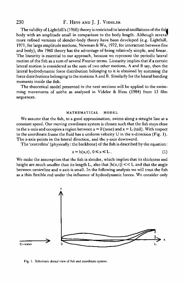
We assume that the fish, to a good approximation, swims along a straight line at aconstant speed. Our moving coordinate system is chosen such that the fish stays closeto the x-axis and occupies a region between x = 0 (nose) and x = L (tail). With respectto the coordinate frame the fluid has a uniform velocity U in the x-direction (Fig. 1).The z-axis points in the lateral direction, and the y-axis downward.

The 'centreline' (physically: the backbone) of the fish is described by the equation:

= h(x,t), 0=£x=SL. (1)

We make the assumption that the fish is slender, which implies that its thickness andheight are much smaller than its length L, also that |h(x,t)| < < L and that the anglebetween centreline and x-axis is small. In the following analysis we will treat the fishas a thin flexible rod under the influence of hydrodynamic forces. We consider only

U—water

Fig. 1. Schematic dorsal view of fish and coordinate system.

Dynamic analysis of swimming 231iateral bending, because it appears to determine completely the variations in bodyshape of a swimming fish with the exception of the tail region and extended fins. Forfast-swimming saithe this approach seems to be justified.

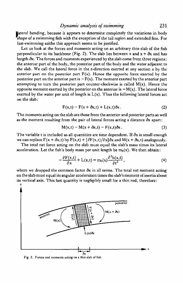
Let us look at the forces and moments acting on an arbitrary thin slab of the fishperpendicular to its backbone (Fig. 2). The slab lies between x and x + 6x and haslength <5x. The forces and moments experienced by the slab come from three regions:the anterior part of the body, the posterior part of the body and the water adjacent tothe slab. We call the lateral force in the z-direction exerted at any section x by theanterior part on the posterior part F(x). Hence the opposite force exerted by theposterior part on the anterior part is — F(x). The moment exerted by the anterior partattempting to turn the posterior part counter-clockwise is called M(x). Hence theopposite moment exerted by the posterior on the anterior is — M(x). The lateral forceexerted by the water per unit of length is L(x). Thus the following lateral forces acton the slab:

F(x,t) - F(x + 6x,t) + L(x,t)5x. (2)

The moments acting on the slab are those from the anterior and posterior parts as wellas the moment resulting from the pair of lateral forces acting a distance <5x apart:

M(x,t) - M(x + <5x,t) - F(x,t)(5x. (3)

The variable t is included as all quantities are time dependent. If <5x is small enoughwe can replace F(x + 6x,t) by F(x,t) + [3F(x,t)/3x]<5x and M(x + 6x,t) analogously.

The total net force acting on the slab must equal the slab's mass times its lateralacceleration. Let the fish's body mass per unit length be mt,(x). We then obtain:

,a2h(x,t)0F(x,t)ax

L(x,t) = mb(x)- (4)

where we dropped the common factor «5x in all terms. The total net moment actingon the slab must equal its angular acceleration times the slab's moment of inertia aboutits vertical axis. This last quantity is negligibly small for a thin rod, therefore:

L(x)<5x

Fig. 2. Forces and moments acting on a thin slab of fish.


The 'internal' force F and moment M vanish at the nose and tail ends:

F(O,t)= F(L,t) = 0, ]

M(0,t) = M(L,t) = 0. J

These end conditions apply whenever the fish moves freely in the water. They wouldbe violated if the fish were attached to some object at either its nose or its tail.

Equation (5) indicates that F = —dM/dx. Substitution into (4) yields:

dy a y (7)For L(x,t), the hydrodynamic lateral force per unit length, we take the followingexpression, as derived by Lighthill (1960) for his small-amplitude slender-bodytheory:

( j U ^ ) { ( f £ ) } (8)where ma(x) is the lateral added mass per unit length and it depends on the local cross-section shape of the fish. The combination of (7) and (8) gives an equation connectingh(x,t) with the bending moment M(x,t). If the lateral motion h(x,t) is given, togetherwith L, U, ma(x) and mt,(x), then the second derivative of the bending momentd2M/dx2, can be obtained and from this follows M(x,t) itself after integrating twice.However, note that whereas we must satisfy four end conditions (6), we can onlyadjust two integration constants. Hence, for an arbitrary lateral motion, at most twoof the four end conditions can be satisfied. This means that only a restricted class oflateral motions h(x,t) is allowed. This restriction is equivalent to the restrictionimposed by the recoil conditions stated by Lighthill (1960).

It should be pointed out that essentially the same mathematical model was outlinedby Wu (1971), who explicitly took elasticity into account and also by Lighthill (privatecommunication in 1978), who treated the fish as an elastic beam. In this paper we donot distinguish between the elastic bending moments and the bending momentsgenerated by the fish's muscles.

Let us now consider the mechanical energy generated and spent by a thin slab atan arbitrary section of the fish. As we are interested in the muscle power required topropel the fish by bending its body, we will first look at the power (= energy per unittime) exerted by the bending moment M(x,t). The mechanical power produced insidethe slab between x and x + dx equals the bending moment times the rate of changeof the slab's curvature:

n*/ \ d 8 h(x.t) £ .„.M(X't)d~t~dx^6x- ( 9 )

Hence, the power produced per unit length equals:

^ (101

Dynamic analysis of swimming 233How is this power spent? Firstly, some power is spent on the slab itself by increasingits kinetic energy:

rdh(xt)12 l ah(xt)d2h(x,t) . . . .^>>. (11)

Secondly, the power spent on the water adjacent to the slab equals (force timesvelocity):

^ M (12)L(x,t)&cat

These two parts, by virtue of (4), add up to

gF(x.tax at

Hence, the power spent per unit length on fish plus water equals:

D / . .^_d2M(x, t )ah(x, t )i Z V M V ax2 at

where we used (5). The difference (Pi(x,t)—Pz(x,t)}6x is the power 'exported' by theslab to the anterior and posterior parts of the fish. At each instant, t, the powergenerated in the whole fish must equal the power spent on the whole fish plus water:

ft P,(x,t)dx = ft P2(x,t)dx = P(t). (15)

For the difference Pi —P2 we have:

P,(x,t)-P2(x,t) = M(x,t)^-ax2 at

(16)IX

where the function R is defined by:

R(x,t) = M(x,t)^--

R(x,t) is the power transported inside the fish across the section at x from anterior toposterior. The first term in the right-hand side of (17) is the power exerted by theanterior part on the posterior part by moment and angular velocity, the second termis the power exerted by the anterior part on the posterior part by force and lateralvelocity. From (16) it follows:

Jg» {P,(x,t) - P2(x,t)}dx = R(xo,t). (18)

If L is substituted for xo, then (15) shows that R(L,t) must vanish. This agrees withthe end conditions (6): both M and dM/dx vanish at x = L and hence R according to(17).

In addition to the power transported inside the fish, as represented by R, there isalso power leaving the fish body and entering adjacent water at some places and


returning to the body elsewhere. The power spent on the water per unit length is givenby (12). Hence, the power transport outside the fish across the plane x = xo is:

dx. (19)

Periodic motion

We now apply the theory of the previous section to the periodic swimming motionas described by Videler & Hess (1984). The time period of the lateral motion is T, andh(x,t) is represented by a Fourier series:

sh(x,t) = .2 (aj(x)cosj(ot + bj(x)sinj<wt}, (O=2n/T, (20)

odd

which can be written in the alternative form:

h(x,t) = .2 w hj(x)co8ja>[t - TJ(X)], (21)

where the hj(x) are amplitude functions and the Tj(x) phase functions. The time originis chosen such that Ti(L) = 0 by definition.

We define the function f by:

^ > (22)

It is the lateral body curvature function, which we can write as:

f(x,t) = .2 3s {ai"(x)cosj(Wt + bj"(x)sinjart}

= i?.^ fi(x)cosj«o[t - oj(x)]. (23)

The Fourier coefficients aj(x) and bj(x) are represented by cubic splines are explainedby Videler & Hess (1984). We have chosen the end conditions of vanishing curvatureat both nose and tail: f(O,t) = f(L,t) = 0. The numerical values for aj"(x) and bj"(x)are obtained by the 'spline-on-spline' method.

Let us represent the lateral bending moment M by:

M(x,t) = 2 i j 5 (pj(x)cosjan + qj(s)sinjcwt}

= 2AsMj(x)cosja)[t-tt(x)]. (24)As

The pj(x) and qj(x) are Fourier coefficients, the Mj(x) amplitude functions and thefi(x) phase functions.

If we substitute (24) and (20) for M(x,t) and h(x,t) in equations (7) and (8) weobtain a set of equations relating the Fourier coefficients aj(x), bj(x) and pj(x), qj(x).Each of the frequencies (j = 1,3,5) can be dealt with separately. After carrying out thenecessary differentiations, we obtain:

Dynamic analysis of swimming 235

Pj"(x) = - jW{m a (x) + mb(x)}aj(x) + Ujft){2ma(x)bj'(x) + ma'(x)bj(x)}

+ U2{ma(x)aj"(x) + ma'(x)aj'(x)}> (25)

qj"(x) = - jW{m a (x) + mb(x)}bj(x) - Uj<o{2ma(x)aj'(x) + ma'(x)aj(x)}

+ U2{ma(x)bj"(x) + ma'(x)bj'(x)}.

Integrating twice yields pj(x) and qj(x), which determine the contribution of the jthfrequency to the bending moment. However, the correct solution requires that bothM and M' vanish at the end points, hence that:

for x = 0 and x = L, j = 1,3,5. (26)

These 'recoil-conditions' will not automatically be satisfied. The next section gives amethod to deal with this problem.

Values for Pi(x,t), Pz(x,t), R(x,t), etc. are obtained by substitution of the ex-pressions (20) and (24) and their derivatives. The mean bending power per unitlength is:

P:(x) = 4 2 i M )(o{Pi(x)W'(x) ~ qj(x)aj"(x)}. (27)

The mean power spent per unit length on fish plus water is:

P2(x) = \ .2 w ja>{Pj"(x)bj(x) - q)"(x)aj(x)} (28)

and the mean internal power transport is:

R(x) = i 2 i w j(u{pj(x)bj'(x) - qj(x)ai'(x) - pj'WbjW + qi'(x)aj(x)}. (29)

According to Lighthill (1960) the mean thrust 0for a periodic motion is given by:

and the mean power delivered by the fish:

+ u !dt J dt ox J X =L

Both 8 and P depend only on what happens at the tail end. The hydrodynamic Froudeefficiency is given by:

rj = 0U/P . (32)

If the lateral motion has the form (20), then we have:

6 = im.(L) 2 ,, {j V ( a j2 + bj2) - U2(a/2 + bj'2)} (33)

j - l . 3 . 5

P = |Uma(L) 2 {j2w2(aj2+ bj2) + j«uU(bjaj' - ajbj')}, (34)


where the values of aj, bj, z\ , b{ are those at x = L.We note that the mean total power P and the mean thrust 6 are the sums of ths

means for each frequency. The fluctuations within one period, however, are the resultof an interplay between the various frequencies.

Rewriting equation (6) from Lighthill (1960), we find for the instantaneous thrust

i I - (35)

where H is defined by

(36)

The time average of the integral in (35) vanishes and the second term yields (30). Thesecond term becomes negative as well as positive during one half period. Our numeri-cal calculations indicate that the first term cancels the strong fluctuations of the secondterm only for a small part.

The higher frequency terms contribute relatively very little to the thrust and totalpower according to our calculations. We therefore paid most attention to the firstfrequency terms; those with j = 1 in the above formulae. For the bending power perunit length, this term can be written as:

Pi(x,t) = £<wfi(x)Mi(x){sin£»[ai(x) - ^(x)] - sinco[2t - ffi(x) - //i(x)]} . (37)

This quantity fluctuates with a period of T/2. Its mean value is determined by thefirst term between the braces, it may be positive or negative depending on the phasedifference between curvature f and bending moment M. The fluctuations are deter-mined by the second term. Pi changes its sign twice per T/2 (except when o\—/iiequals an odd multiple of T/4, then Pi just touches zero). Pi has a positive mean valueif

k T < a i ( x ) - / * i ( x ) < ( k + l / 2 ) T , (38)

where k is any integer. The higher frequency contributions may influence the fluctua-tions of Pi , but for any periodic motion Pi(x,t) is negative as well as positive in thecourse of one period, because Pi is the product of two quantities, M and dh"/3t,which both change their signs periodically and generally not simultaneously. Thismeans that at any cross section of the fish the power associated with the bendingmoment fluctuates around its local mean value, inevitably becoming negative or zeroduring part of the period.

For the power spent on fish plus water P2(x,t) (equation 14) expressions similar tothose for Pi can be derived. In the periodic case the time average l?2(x) is the meandifferential power spent on the water, because the mean power spent on the bodyvanishes.

Recoil correction

We now must regard a crucial but rather inconvenient point: recoil. As mentionedbefore, the fish's motion must be such that the end conditions (6) are satisfied. Ourfunctions h(x,t) do not satisfy these conditions for two main reasons: firstly, the lateraj


(potion h(x,t) as well as the mass functions mb(x) and ma(x) are not exact, but containome errors. And, secondly, a real fish (such as saithe) is not a true slender body,

hence the hydrodynamic forces computed on the basis of Lighthill's (1960) theory arenot exact. Now we are faced with the problem of applying some sort of recoil correc-tion to h(x,t) to make it satisfy the conditions (26) for the periodic case. There aremany ways in which this could be done. We use one that is relatively simple, but notnecessarily the best. We allow a certain amount of stiff motion A(t) + xB(t) to beadded to h(x,t). In this manner the curvature f(x,t) is not affected. This stiff motionis represented by:

A(t) + xB(t) = . xr2j)cosftrt + (r3j + xr4j)sinart}. (39)

(40)

C3r4j,(41)

For this motion we obtain, in analogy with (24):

Pj"(x) = —j2<w2{ma(x) + mb(x)}(rij + xr2j) + j<oU{2ma(x)r4j

+ ma'(x)(r3j + xr4j)} + U2ma'(x)r2j,

qj"(x) = -jW{ma(x) + mb(x)}(r3j + xr4j) - jeoU{2ma(x)r2j

+ ma'(x)(rij 4- xr2j)} + U2ma'(x)r4j

for j = 1, 3, 5. After integrating twice, we get:

Pj'(L) = +Cirij + C2r3j + C3r2j + C4r4j,

qj'(L) = -C2rij + Cir3j — C4r2j

Pj(L) = +Csrij + C6r3j + C?r2j -\

qj(L) = —C6rij + Csr3j — Csr2j H

The coefficients Ci through Cg can be computed from the functions ma(x) and mb(x)by numerical integration

Ci = - j W J0L {ma(x) + mb(x)}dx

C2 = jwUma(L)

C3 = -j2ft>2 ft {ma(x) + mb(x)}xdx + Uma(L)

C4 = jft>U {ftma(x)dx + Lma(L)}

Cs = -}W ft ft' {ma(x) + mb(x)}dxdx'

C6 = ]CO\J ft ma(x)dx

C7 = - j V [ft ft' (ma(x) + mb(x)}xdxdx' + U2 ft ma(x)dx]

C8 = jwU {ft Jo' ma(x)dxdx' + ft ma(x)xdx}.

We proceed as follows. First we solve equations (7) and (8) for M"(x,t) using theoriginal h(x,t) as derived from the film sequences. By twice integrating (25) we obtainPj'(L), qj'(L), pj(L), qj(L). The values atx = 0 vanish automatically. We want to addthe appropriate amount of stiff motion. (Here the linearity of the theory is crucial.)ffhen the equations (41) must be solved for rij, r2j, r3j and r4j with the left-hand sides

(42)


set equal to minus the corresponding quantities obtained from h(x,t). We then adthe resulting stiff motion (39) to h(x,t). A similar treatment of recoil is given bLighthill (1970).

This concludes the description of the mathematical model. The numerical calcula-tions are carried out by evaluating the integrands at 101 equidistant points, andapplying the trapezium rule on each of the 100 segments. The computing programmeare written in Basic and run on an HP9835A computer.

Dimensionless quantities

We shall express the physical quantities in dimensionless form, because this makesit easier to compare cases differing in size or swimming speed. The resistance or dragD which the fish must overcome when moving forward is often expressed as:

D = £pU2AwCD, (43)

where CD is the dimensionless drag coefficient, and Aw the wetted surface area of thefish, g is the density of water and also the mean density of the fish. Similarly the thrustcoefficient CT is connected with the thrust 6:

0 = £pU2AwCT. (44)

If the Reynolds number is high enough (so that viscous effects are restricted to a thinboundary layer on the body surface), CD depends only on the body shape of the fish,not on absolute size or speed. If thrust and drag are not equal in magnitude, then thefish accelerates or decelerates:

(45)

where mf is the fish's volume. From this follows:

„ n mf UL a , . , .CT~CD = IA^TF=SP- (46)

The first factor is the dimensionless shape parameter s, and the second factor is thedimensionless acceleration parameter /S (see Videler & Hess. 1984). Just as in thatpaper we shall use the time period T as a unit of time and the fish length L as a unitof length. Further we choose the mass of a volume L3 of water as a mass unit. In theseunits we have: L = l , T = 1, g= 1 and a) = 2.K. To convert to conventional units,lengths must be multiplied by L, times byT, velocities by LT"1 , forces by pL4 T~2,moments by pLsT~2, powers by pL5T~3, powers per unit length by pL4T~3, massper unit length by £>L2, etc.

Body shape of saithe

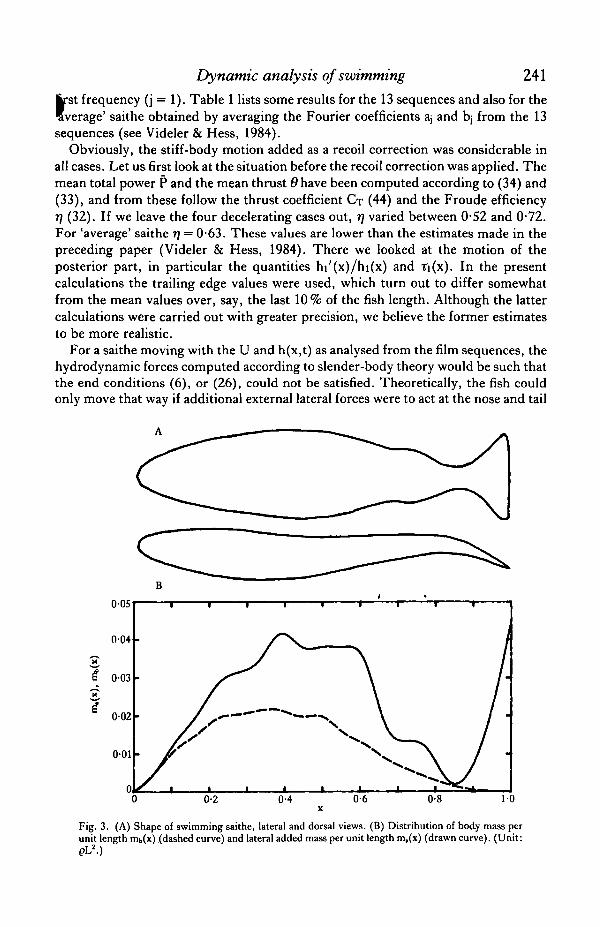
Fig. 3A shows the dorsal and lateral views of a swimming saithe as drawn from cin£pictures. Fig. 3B presents graphs for the body mass distribution mb and thehydrodynamic lateral added mass distribution nia • All quantities are made dimension-less as outlined above. The cross-sectional shape of saithe was determined by measur-ing three specimens (length about 0-22 m each). Cin6 pictures were used to determinethe shape of the tail fin during regular swimming, and to verify that the other fins wer'a

Dynamic analysis of swimming 239completely collapsed. The body mass per unit length mt,(x) and the lateral

ded mass per unit length ma(x) were calculated by:

ma = iwh2 '

where b is the local body width, hi the local body height excluding fins and h2including fins. Both formulae are valid for elliptical sections. Lighthill (1970) showedthat deviations from the calculated ma values are likely to be small. After b, hi, Ii2 weredetermined at some 18 points, smooth functions mt,(x) and rria(x) were obtained byinterpolation with cubic splines.

Some relevant quantities are:

Height of tail fin at trailing edgeAdded mass at trailing edgeBody volumeWetted areaShape parameter, see (45)Reynolds number (Re)

0-24 [L]ma(L) =mf =

A w =s =between 2 X

0-0452 [L2]0-0113 [ i /0-401 [L2]0-056410s and 8 X

We may well pose the question: how closely does a saithe resemble a slender body?One may think of slender-body theory as an approximate theory whose resolvingpower is limited to details in space which have about the size of the cross-sectionaldimensions of the 'slender' body. In our case that means roughly one-quarter of thefish length, which is not very good. (For eel it would be about one-tenth, which ismuch better.) In slender-body theory the mean thrust and the mean total powerdepend only on what happens at the tail end, but the theory implies that what happensjust ahead of the tail end is not very different. Here 'just ahead' may mean an area aslarge as the whole fish tail in saithe. However, the height, for instance, varies stronglyalong the tail. From this it is clear that the numerical results presented in this papershould be considered as approximate estimates rather than as precise quantitativepredictions.

It is quite likely that slender-body theory over-estimates the hydrodynamic forces,especially at the tail. Firstly, as pointed out by Lighthill (1970), the effective lateraladded mass is smaller if the body wave length is not very much (say, at least five times)greater than the body height. Secondly, the tail region of saithe is not slender, strictlyspeaking. The tailfin roughly resembles a triangular wing of aspect ratio 4 (Fig. 3A).For such a wing in steady flow the lift is over-predicted by a factor of 1-8 by slender-body (or rather slender-wing) theory (Lawrence, 1951). The only remedy would beto employ some kind of unsteady lifting-surface theory, but that would involvetremendous complications in comparison with Lighthill's (1960) elegant slender-bodytheory.

RESULTS AND DISCUSSION

The third and fifth frequencies (j = 3, 5 in the formulae) each contributed onlyibout 1 % to the power and the thrust (Fig. 6). Therefore, we shall deal only with the

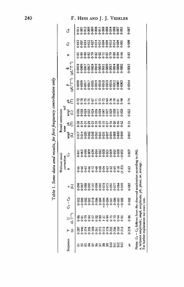
Dynamic analysis of swimming 241fcst frequency (j = 1). Table 1 lists some results for the 13 sequences and also for theliverage' saithe obtained by averaging the Fourier coefficients z\ and bj from the 13sequences (see Videler & Hess, 1984).

Obviously, the stiff-body motion added as a recoil correction was considerable inall cases. Let us first look at the situation before the recoil correction was applied. Themean total power P and the mean thrust 6 have been computed according to (34) and(33), and from these follow the thrust coefficient Or (44) and the Froude efficiencyT} (32). If we leave the four decelerating cases out, r} varied between 0-52 and 0-72.For 'average' saithe T] = 0-63. These values are lower than the estimates made in thepreceding paper (Videler & Hess, 1984). There we looked at the motion of theposterior part, in particular the quantities hi'(x)/hi(x) and Ti(x). In the presentcalculations the trailing edge values were used, which turn out to differ somewhatfrom the mean values over, say, the last 10% of the fish length. Although the lattercalculations were carried out with greater precision, we believe the former estimatesto be more realistic.

For a saithe moving with the U and h(x,t) as analysed from the film sequences, thehydrodynamic forces computed according to slender-body theory would be such thatthe end conditions (6), or (26), could not be satisfied. Theoretically, the fish couldonly move that way if additional external lateral forces were to act at the nose and tail

Fig. 3. (A) Shape of swimming saithe, lateral and dorsal views. (B) Distribution of body mass perunit length mb(x) (dashed curve) and lateral added mass per unit length m,(x) (drawn curve). (Unit:pL2.)


ends. We computed these virtual forces. In all cases the external force at the tail enMcounteracted the computed hydrodynamic force, whereas the additional force at th?nose end was much smaller. Let us take the case of 'average' saithe. The virtual force onthe nose end had an amplitude 0-002 (pL4T~2) and reached its maximum at t = 0-33(T). The virtual lateral force on the tail end had an amplitude 0 • 0063, and its maximumoccurred at t = 0-90. Now, the lateral hydrodynamic force acting on the fish betweenx = 0-95 and x = 100 had an amplitude 00061 and reached its maximum at t = 0-36,that is 0-54 T earlier than the virtual force. Thus the computed hydrodynamic force onthe last 5 % of the fish length was cancelled for a great part by the virtual force. Thisclearly shows that the saithe can only carry out its observed movement if thehydrodynamic force on the tail is much smaller in reality than as computed.

The stiff-body motion added as recoil correction is indicated in Table 1 by thevalues of its amplitude and phase at the nose and tail ends. Fig. 4 provides a com-parison between the lateral motion before and after recoil correction for 'average'saithe. The amplitudes at nose and tail ends were hardly affected, but in between the'corrected' amplitude was higher. The most significant change concerned the tailregion, where hi'(x) was much reduced after the correction. The 'corrected' phasefunction Ti(x) equalled -0-043 at the tailing edge rather than zero. The wave speedV (= 1/TI') was only marginally increased in the tail region, but its overall value washigher. Before recoil correction we have V = 1-04, U/V = 0-82, and after recoil cor-rection V = 1-26, U/V = 0-68 over the posterior half of the fish.

014

012 -

-1-4

Fig. 4. Lateral motion of 'average' saithe before recoil correction (drawn curves) and after recoilcorrection (dashed curves). First frequency contribution only. Nose is at x = 0, tail point at x = 1.Left: amplitude functions h^x) (unit: L). Right: phase functions r,(x) (unit: T).

Dynamic analysis of swimming 243Values for P, 6, Or and r\ after recoil correction are listed in Table 1. From the

Observed acceleration C T ~ CD follows according to (46). This leads to the drag co-efficient values in the last column of Table 1. The Froude efficiency r) ranged from0-65 to 0*84, or, if the four decelerating cases are left out, from 0-79 to 0-84. CT variedbetween 0-001 for the decelerating S13 to 0-027 for the rather strongly acceleratingS5. CD varied between 0-003 and 0014. For 'average' saithe we find CT = 0-009 and,as the average value for CT—CD = 0-002, we estimate CD = 0-007. The mean totalpower P for 'average' saithe was 0-0014 (pL5T~3), which corresponds to about0-7 W kg"1 body weight. (For SS it is about 3-5 W kg"1.)

The calculated thrust 6 fluctuated during each half-period between zero andapproximately twice its average value 6. For 'average' saithe 6 = 0-0013 ± 0-0011. Ifthe drag on the fish were constant, such thrust fluctuations would cause oscillationsof the forward speed about its mean value U. According to (46) the fluctuations in Uwould have an amplitude:

^ (48)

This gives rise to relative speed fluctuations with amplitude:

AU _ A C T U

U scoL '(49)

where A Or is the amplitude of the fluctuations in the thrust coefficient. For 'average'saithe (49) yielded about 2 %, and the maximum thrust occurred at t — —0-24 whichwas nearly simultaneous with the maximum bending moment, roughly when the tailpoint passes the plane z = 0. These fluctuations are somewhat stronger than thoseobserved in the preceding paper (Videler & Hess, 1984). In the accelerating case S5we find AU/U — 5 %, which agrees with the observed value. The computed instantof maximum thrust was at t = —0-28, whereas the kinematic data yielded t = —0-20.

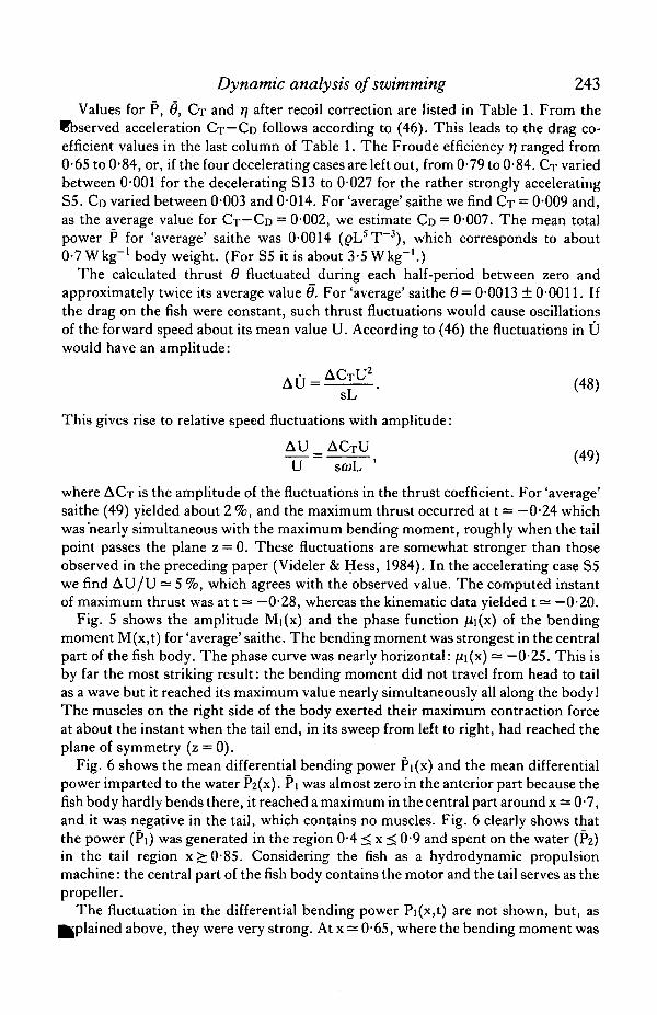
Fig. 5 shows the amplitude Mi(x) and the phase function jUi(x) of the bendingmoment M(x,t) for 'average' saithe. The bending moment was strongest in the centralpart of the fish body. The phase curve was nearly horizontal: fii(x) — —025. This isby far the most striking result: the bending moment did not travel from head to tailas a wave but it reached its maximum value nearly simultaneously all along the body!The muscles on the right side of the body exerted their maximum contraction forceat about the instant when the tail end, in its sweep from left to right, had reached theplane of symmetry (z = 0).

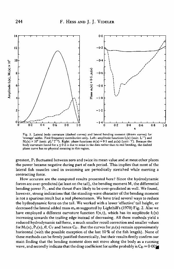
Fig. 6 shows the mean differential bending power Pi(x) and the mean differentialpower imparted to the water P2(x). Pi was almost zero in the anterior part because thefish body hardly bends there, it reached a maximum in the central part around x = 0-7,and it was negative in the tail, which contains no muscles. Fig. 6 clearly shows thatthe power (Pi) was generated in the region 0-4 < x < 0-9 and spent on the water (P2)in the tail region x>0-85. Considering the fish as a hydrodynamic propulsionmachine: the central part of the fish body contains the motor and the tail serves as thepropeller.

The fluctuation in the differential bending power Pi(x,t) are not shown, but, as^plained above, they were very strong. At x = 0-65, where the bending moment was


o

X

S 8 "

S 6-T3

"E.

-1-4

Fig. 5. Lateral body curvature (dashed curves) and lateral bending moment (drawn curves) for'average' saithe. First frequency contribution only. Left: amplitude functions fi(x) (unit: L"1) andM|(x) X 104 (unit: pL5T~z). Right: phase functions ai(x) + 0S and fii(x) (unit: T). Because thebody curvature found for x < 0-2 is due to noise in the data rather than to real bending, the dashedphase curve has no physical meaning in this region.

greatest, Pi fluctuated between zero and twice its mean value and at most other placesthe power became negative during part of each period. This implies that most of thelateral fish muscles used in swimming are periodically stretched while exerting acontracting force.

How accurate are the computed results presented here? Since the hydrodynamicforces are over-predicted (at least on the tail), the bending moment M, the differentialbending power Pi, and the thrust 0are likely to be over-predicted as well. We found,however, strong indications that the standing-wave character of the bending momentis not a spurious result but a real phenomenon. We have tried several ways to reducethe hydrodynamic force on the tail. We worked with a lower 'effective' tail height, ordecreased the lateral added mass ma as suggested by Lighthill's (1970) Fig. 2. Also wehave employed a different curvature function f(x,t), which has its amplitude fi(x)increasing towards the trailing edge instead of decreasing. All these methods yield areduced hydrodynamic tail force, a much smaller recoil correction and smaller valuesforMi(x), Pi(x), 6, CT and hence CD . But the curves for /ii(x) remain approximatelyhorizontal (with the possible exception of the last 10% of the fish length). None ofthese methods can be firmly justified theoretically, but their results firstly confirm ourmain finding that the bending moment does not move along the body as a runningwave, and secondly indicate that the drag coefficient for saithe probably is CD — 0-00 j |


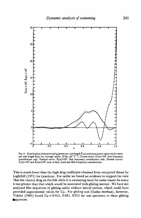
Fig. 6. Distribution of mean bending power per unit length Pi (x) and mean power spent on the waterper unit length ?2(x) for 'average' saithe. (Unit: pL4T ). Drawn curve: Pi(x)x lCr, first frequencycontribution only. Dashed curve: P2(x)XlO3, first frequency contribution only. Dotted curves:Pi(x) X103 and Pz(x)X103, sum of first, third and fifth frequency contributions.

This is much lower than the high drag coefficient obtained from computed thrust byLighthill (1971) for Leuciscus. For saithe we found no evidence to support his view'that the viscous drag on the fish while it is swimming must for some reason be manyti mes greater than that which would be associated with gliding motion'. We have notanalysed film sequences of gliding saithe without lateral motion, which could haveprovided experimental values for CD . For gliding cod (Gadus morhua), however,Videler (1981) found CD = 0-015, 0-011, 0-011 for one specimen in three glidingSequences.


Our findings are supported by preliminary results of a similar analysis of the swim|ming motion of eel {Anguilla anguilla). Hydrodynamically an eel behaves as a slendeiibody to a good approximation. Indeed, the recoil corrections required for eel aremuch smaller than for saithe. The bending moment has the same character, althoughthe phase function jUi(x) in eel is not quite so constant as in saithe. The mean differen-tial bending power Pi has roughly the same shape as in saithe, but the negative peakin the tail region is relatively more pronounced in eel. All these results are qualitativelysimilar to those presented here for saithe.

In deriving the major result, the 'standing wave' character of the bending moment,we started from a running wave of body curvature. And indeed, the swimmingstrategy of a fish might be to send waves of curvature along its body from head to tail.However, our findings indicate that a fish may well use the strategy of exertingbending forces simultaneously throughout its body, alternately using the muscles onthe left side and on the right side. The running wave in its body shape is then the resultof the interaction with the water flow. If this hypothesis is correct, the running waveshould be absent if a fish starts from stand-still in water or moves in air, provided thefish produces the same muscle force. Our view is supported by Hertel's (1963) Fig.169 of a trout starting and swimming, and also by Fig. 2 of Weihs (1973) of a troutaccelerating from stand-still.

The use of lateral muscles in swimmingThe results of our dynamic analysis provide new insight into the function of the

lateral muscles for swimming. We shall first give a short description of the relevantstructures of saithe and then discuss the implications of our findings with respect tomuscle function.

Mechanically important parts of the locomotory apparatus used for continuousswimming include the vertical septum, and left and right lateral muscles, surroundedby the skin and the tailblade. The anatomy of these structures closely resembles thatfor cod, which is described by Wardle & Videler (1980) and Videler (1981). Thevertical septum between the back of the head and the tailblade divides the body intotwo lateral halves. It is a sheet of collagenous fibres supported by the vertebralcolumn. Mechanically the vertebral column can be regarded as an inextensible andincompressible flexible rod, easily bent in the horizontal plane. The connectingtissues between the vertebrae give the column self-restoring elastic properties (Sym-mons, 1979). The lateral muscles are metamerically arranged in myotomes separatedby myosepts, both structures with a complicated geometry. The muscle fibres areattached to the myosepts and run approximately in the direction of the longitudinalbody axis. Myosepts are attached to the vertical septum and at certain places to theskin. There is a thin layer of red aerobic muscle fibres on the outside of the myotomesjust under the skin. The bulk of muscle fibres is white and works anaerobically. Thelateral muscles are also firmly attached to the head and on the other end of the fish tothe fin ray heads of the tailblade. From just behind the head (at x — 0-2) to the positionof the anus (at x = 0-45) the ventral part of the fish contains the abdominal cavity. Athin layer of lateral muscles supported by ribs surrounds this cavity, and the lateralbending is restricted in this region. From the anus to the caudal end of the body themyotomes are bilaterally and dorsoventrally symmetrical.

Dynamic analysis of swimming 247The skin is a strong structure of layers of collagenous fibres in criss-cross arrange-

ment (Videler, 1975). It is attached to the head and to the vertical septum along thedorsal and ventral rim and it inserts firmly on to the fin ray heads of the tailblade. Thestructure of the joints between the fin rays of the tailfin and the caudal peduncle allowsthe fish to keep the bending properties of the tailblade under muscular control. Detailswere given by McCutchen (1970) and Videler (1977, 1981). The curvature of thetailblade will be the result of elastic properties of the fin rays, controlled by intrinsicmusculature in the peduncle and by lateral musculature via the skin, in interactionwith bending forces exerted by the water.

The body curvature is connected with variations in length of the muscle fibres oneither side of the septum. In our frame of reference, a positive curvature means thatthe fibres on the right side are shorter than their resting length, and those on the leftside longer; for negative curvature it is the other way around. A positive bendingmoment implies that the muscles on the right side exert a contraction force and thoseon the left side are passive or exert a smaller contraction force. We simplify our lineof reasoning by making the assumption that all the contraction forces are exerted byfibres lying at a distance from the septum d(x) = ib(x) where b is the lateral thickness.This is approximately where the red muscle fibres are situated, and the simplifiedsituation may not be too unrealistic during swimming at cruising speeds when mostof the bending moment is generated by the red muscles. However, our assumptionmainly serves as an instructive device.

The relative length change A/// of the chosen fibres on the right side of the fishfollows from the curvature h":

Ad(x,t) = - y = h"(x,t)d(x), (50)

where Ad is the relative shortening of the fibres. On the left side of the fish A/// hasthe opposite sign. If the bending moment is generated by forces in the chosen fibresthen the force Fa(x,t) follows from

Fd(x,t) = M(x,t)/d(x). (51)

If M is positive then the contraction force Fd is exerted by the fibres on the right side,if M is negative then the contraction force — Fd is exerted by the left-side muscles. Thepower produced by the hypothetical muscle fibres per unit length is given by:

Fd(x,t)|-Ad(x,t) = M(x,t)^-h"(x,t) = Pi(x,t). (52)ot ot

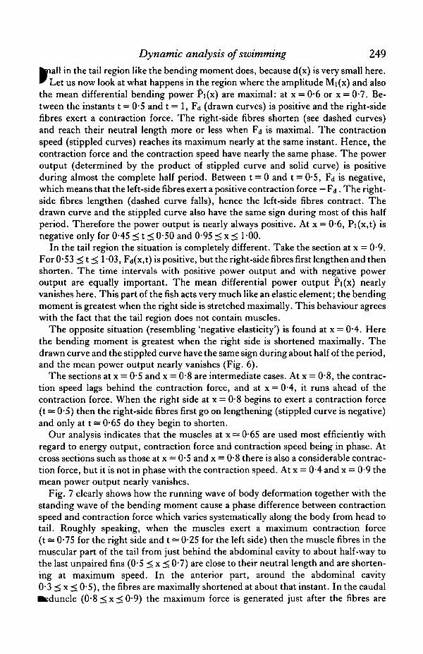
In Fig. 7 the functions Fd , Ad and -̂ -Ad are plotted as a function of time during oneot

period for several cross sections along the fish body: x = 0-1(0*1)0-9. At the nose andtail points (x = 0, x = 1) both Fd and Ad vanish. The relative fibre length shorteningAd(x,t) is represented by the dashed curves. The extreme values reached are plus andminus 6 %. In the tail region (x = 0-9) the curvature is large (Fig. 5) but the bodythickness is small, and Ad varies between plus and minus 4%. The curve at x = 0 1is probably caused by noise in the kinematic data, since the fish's head is rigid. The

•entraction force Fd(x,t) is represented by the drawn curves. It does not become very


01

0-2

0-3

0-4

* 0-5

0-6

0-7

0-9

•f >r" i ' 1-

0-5t

1-0

Fig. 7. Contraction force, relative length change and contraction speed in outer fibres (see main textfor explanation) during one complete period at nine different sections of 'average' saithe. Firstfrequency contribution only. Numbers at left indicate x-positions of sections. At x = 0 (nose) andx = 1 (tailpoint) all curves vanish. Drawn curves: contraction force in outer fibres, if positive then onthe right side, if negative then on the left side. One vertical division equals 002pL 4 T~ z . Dashedcurves: relative shortening of outer fibres, if positive then the right-side fibres are shortened and theleft-side fibres are lengthened. One vertical division equals 0-02 ( = 2 % length change). Dottedcurves: contraction speed (that is the rate of change of relative shortening), if positive then the right-side fibres shorten. One vertical division equals 0*1 T"1. The bending power P|(x,t) at each sectionis obtained by multiplying the drawn curve by the dotted curve.


knall in the tail region like the bending moment does, because d(x) is very small here." Let us now look at what happens in the region where the amplitude Mi(x) and alsothe mean differential bending power Pi(x) are maximal: at x = 0-6 or x = 0-7. Be-tween the instants t = 0-5 and t = 1, Fd (drawn curves) is positive and the right-sidefibres exert a contraction force. The right-side fibres shorten (see dashed curves)and reach their neutral length more or less when Fd is maximal. The contractionspeed (stippled curves) reaches its maximum nearly at the same instant. Hence, thecontraction force and the contraction speed have nearly the same phase. The poweroutput (determined by the product of stippled curve and solid curve) is positiveduring almost the complete half period. Between t = 0 and t = 0*5, Fd is negative,which means that the left-side fibres exert a positive contraction force — Fd . The right-side fibres lengthen (dashed curve falls), hence the left-side fibres contract. Thedrawn curve and the stippled curve also have the same sign during most of this halfperiod. Therefore the power output is nearly always positive. At x = 0*6, Pi(x,t) isnegative only for 0-45 < t < 0-50 and 0-95 < x < 1-00.

In the tail region the situation is completely different. Take the section at x = 0-9.For 0-53 < t < 1-03, Fd(x,t) is positive, but the right-side fibres first lengthen and thenshorten. The time intervals with positive power output and with negative poweroutput are equally important. The mean differential power output Pi(x) nearlyvanishes here. This part of the fish acts very much like an elastic element; the bendingmoment is greatest when the right side is stretched maximally. This behaviour agreeswith the fact that the tail region does not contain muscles.

The opposite situation (resembling 'negative elasticity') is found at x = 0-4. Herethe bending moment is greatest when the right side is shortened maximally. Thedrawn curve and the stippled curve have the same sign during about half of the period,and the mean power output nearly vanishes (Fig. 6).

The sections at x = 0-5 and x = 0-8 are intermediate cases. At x = 0*8, the contrac-tion speed lags behind the contraction force, and at x = 0-4, it runs ahead of thecontraction force. When the right side at x = 0-8 begins to exert a contraction force(t = 0*5) then the right-side fibres first go on lengthening (stippled curve is negative)and only at t = 0-65 do they begin to shorten.

Our analysis indicates that the muscles at x = 0-65 are used most efficiently withregard to energy output, contraction force and contraction speed being in phase. Atcross sections such as those at x = 0-5 and x = 0-8 there is also a considerable contrac-tion force, but it is not in phase with the contraction speed. At x = 0-4 and x = 0-9 themean power output nearly vanishes.

Fig. 7 clearly shows how the running wave of body deformation together with thestanding wave of the bending moment cause a phase difference between contractionspeed and contraction force which varies systematically along the body from head totail. Roughly speaking, when the muscles exert a maximum contraction force(t = 0-75 for the right side and t = 0-25 for the left side) then the muscle fibres in themuscular part of the tail from just behind the abdominal cavity to about half-way tothe last unpaired fins (0-5 < x < 0-7) are close to their neutral length and are shorten-ing at maximum speed. In the anterior part, around the abdominal cavity0*3 < x < 0-5), the fibres are maximally shortened at about that instant. In the caudal•tduncle (0-8 < x < 0-9) the maximum force is generated just after the fibres are


maximally stretched. In this region a substantial part of the bending momentprobably due to elastic structures. Indeed, there are no lateral muscles in thebeyond x = O9. Fig. 7 confirms that the section at x = 0-9 shows a purely elasticbehaviour.

The systematic differences in the use of lateral muscles along the body lead one toexpect physiological or morphological adaptations to the different ways of contrac-tion. There are no experimental indications as yet of such physiological differencesbetween muscle fibres. The shape of the myotomes varies along the body but it is stillnot clear how this is related to our results.

Our analysis predicts that the muscle fibres on one side of the fish are simultaneous-ly active. Consequently we expect myograms to occur simultaneously all along oneside of the body. Such patterns have been found experimentally, and indeed Blight(1977) suggests that the running waves of lateral bending can be produced by 'alterna-tions of tension development from side to side'. Blight (1976) finds instantaneousmyograms along one side of swimming palmate newt larvae (Triturus helveticus) andin the same paper presents myogram patterns along the body of a swimming tench{Tinea tinea). His Fig. 4 indicates that the maximum muscle activity along the rightside of the body occurs when the tail tip crosses the plane of symmetry from left toright, which agrees with our results. There is a small time delay between the muscleactivity in the anterior and posterior part, the ending of the activity of the muscles justbehind the head coincides with the beginning of activity in the caudal peduncle. Thevelocity of the wave of contraction is half as fast as the velocity of the wave of cur-vature. Grillner & Kashin (1976) find the wave of electric activity in the eel to beslower than the mechanical wave of bending. Kashin, Feldman & Orlovsky (1979)provide electromyographical evidence for a constant time lag between activation ofanterior and posterior red muscles of the carp during sustained swimming and forsimultaneous activation of homolateral segments during bursts of fast swimming. Theabove myographic data support our view of the use of lateral muscles in swimming.

This work is sponsored by the Foundation for Fundamental Biological Research(BION), which is subsidized by the Netherlands Organization for the Advancementof Pure Research (ZWO).

R E F E R E N C E S

BLIGHT, A. R. (1976). Undulatory swimming with and without waves of contraction. Nature, Land. 264,352-354.

BLIGHT, A. R. (1977). The muscular control of vertebrate swimming movements. Bio/. Rev. 52, 181-218.GRILLNER, S. & KASHIN, S. (1976). On the generation and performance of swimming in fish. In Neural Control

of Locomotion, (eds R. M. Herman, S. Grillner, P. S. G. Stein & D. G. Stuart), pp. 181-201. New York:Plenum Press.

HERTEL, H. (1963). Struktur, Form, Bewegung. Mainz: Krausskopf.KASHIN, S. M., FELDMAN, A. G. & ORLOVSKY, G. N. (1979). Different modes of swimming of the carp,

Cyprinus carpio L.J. Fish Biol. 14, 403-405.LAWRENCE, H. R. (1951). The lift distribution on low aspect ratio wings at subsonic speeds. J. aeronautical

Set. 18, 683-695.LIGHTHILL, M. J. (1960). Note on the swimming of slender fish. J. FluidMech. 9, 305-317.LIGHTHILL, M. J. (1970). Aquatic animal propulsion of high hydrodynamic efficiency. J . Fluid Mech. 44,

265-300. ~~


K:GHTHILL, M. J. (1971). Large-amplitude elongated-body theory of fish locomotion. Proc. R. Soc. B 179,125-138.CCUTCHEN, C. W. (1970). The trout tail fin: A selfcambering hydrofoil. J Biomech. 3(3), 271-281.

NEWMAN, J. N. & Wu, T. Y. (1972). A generalized slender-body theory for fish-like forms. J. FluidMech. 57,673-693.

SYMMONS, S. (1979). Notochordal and elastic components of the axial skeleton of fish and their function inlocomotion. J Zool., Land. 189, 157-206.

VIDELER, J. J. (1975). On the interrelationships between morphology and movement in the tail of the cichlidfish Tilapia nilotica (L.). Neth.J. Zool. 25, 143-194.

VIDELER, J. J. (1977). Mechanical properties of fish tail joints. Fortschr. Zool. 28, 465-484.VIDELER, J. J. (1981). Swimming movements, body structure and propulsion in Cod Gadus morhua. Symp.

Zool. Soc, Land. 48, 1-27.VIDELER, J. J. & H E S S , F. (1984). Fast continuous swimming of two pelagic predators, saithe (Pollachius virens)

and mackerel (Scomber scombrus): a kinematic analysis. J . exp. Biol. 109, 209-228.WARDLE, C. S. & VIDELER, J. J. (1980). Fish swimming. In Aspects of Animal Movement, (eds H. T. Elder

& E. R. Trueman). Soc. exp. Biol. Sem. 5, 125-150. Cambridge: Cambridge University Press.WEIHS, D. (1973). The mechanism of rapid starting of slender fish. Biorheology 10, 343—350.Wu, T. Y. (1971). Hydromechanics of Swimming Fishes and Cetaceans. Adv. appl. Math. 11, 1-63.

fast continuous swimming of saithe …jeb.biologists.org/content/jexbio/109/1/229.full.pdfj. exp....

Documents